Score-Based Generative Modeling through Stochastic Differential Equations

Yang Song$^{*}$
Stanford University
[email protected]

Jascha Sohl-Dickstein
Google Brain
[email protected]

Diederik P. Kingma
Google Brain
[email protected]

Abhishek Kumar
Google Brain
[email protected]

Stefano Ermon
Stanford University
[email protected]

Ben Poole
Google Brain
[email protected]

$^{*}$ Work partially done during an internship at Google Brain.

Abstract

Creating noise from data is easy; creating data from noise is generative modeling. We present a stochastic differential equation (SDE) that smoothly transforms a complex data distribution to a known prior distribution by slowly injecting noise, and a corresponding reverse-time SDE that transforms the prior distribution back into the data distribution by slowly removing the noise. Crucially, the reverse-time SDE depends only on the time-dependent gradient field (a.k.a, score) of the perturbed data distribution. By leveraging advances in score-based generative modeling, we can accurately estimate these scores with neural networks, and use numerical SDE solvers to generate samples. We show that this framework encapsulates previous approaches in score-based generative modeling and diffusion probabilistic modeling, allowing for new sampling procedures and new modeling capabilities. In particular, we introduce a predictor-corrector framework to correct errors in the evolution of the discretized reverse-time SDE. We also derive an equivalent neural ODE that samples from the same distribution as the SDE, but additionally enables exact likelihood computation, and improved sampling efficiency. In addition, we provide a new way to solve inverse problems with score-based models, as demonstrated with experiments on class-conditional generation, image inpainting, and colorization. Combined with multiple architectural improvements, we achieve record-breaking performance for unconditional image generation on CIFAR-10 with an Inception score of 9.89 and FID of 2.20, a competitive likelihood of 2.99 bits/dim, and demonstrate high fidelity generation of $1024\times 1024$ images for the first time from a score-based generative model.

1. Introduction

Section Summary: Score-based generative models, like those in SMLD and DDPM, work by gradually adding noise to training data and then training systems to remove it step by step, allowing the creation of new data such as images or audio. This paper introduces a unified framework that views this noise-adding process as a continuous diffusion over time using stochastic differential equations, where data turns into random noise in the forward direction and noise reshapes into data in the reverse, guided by a neural network estimating probability gradients. This approach enables flexible sampling methods, controllable generation without retraining, and state-of-the-art results, such as high-quality 1024x1024 images and top scores on image datasets like CIFAR-10.

Two successful classes of probabilistic generative models involve sequentially corrupting training data with slowly increasing noise, and then learning to reverse this corruption in order to form a generative model of the data. Score matching with Langevin dynamics (SMLD) ([1]) estimates the score (i.e, the gradient of the log probability density with respect to data) at each noise scale, and then uses Langevin dynamics to sample from a sequence of decreasing noise scales during generation. Denoising diffusion probabilistic modeling (DDPM) ([2, 3]) trains a sequence of probabilistic models to reverse each step of the noise corruption, using knowledge of the functional form of the reverse distributions to make training tractable. For continuous state spaces, the DDPM training objective implicitly computes scores at each noise scale. We therefore refer to these two model classes together as score-based generative models.

Score-based generative models, and related techniques ([4, 5, 6]), have proven effective at generation of images ([1, 7, 3]), audio ([8, 9]), graphs ([10]), and shapes ([11]). To enable new sampling methods and further extend the capabilities of score-based generative models, we propose a unified framework that generalizes previous approaches through the lens of stochastic differential equations (SDEs).

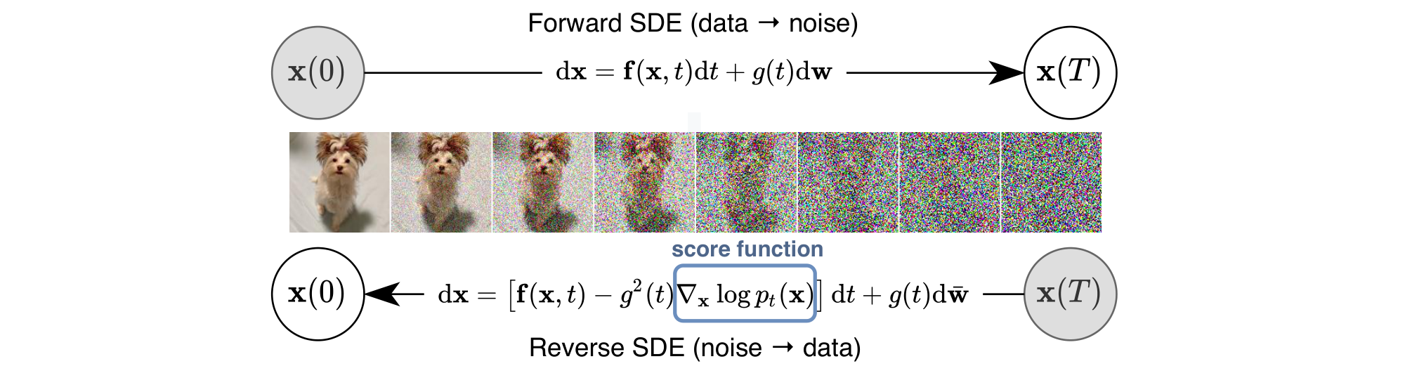
Specifically, instead of perturbing data with a finite number of noise distributions, we consider a continuum of distributions that evolve over time according to a diffusion process. This process progressively diffuses a data point into random noise, and is given by a prescribed SDE that does not depend on the data and has no trainable parameters. By reversing this process, we can smoothly mold random noise into data for sample generation. Crucially, this reverse process satisfies a reverse-time SDE ([12]), which can be derived from the forward SDE given the score of the marginal probability densities as a function of time. We can therefore approximate the reverse-time SDE by training a time-dependent neural network to estimate the scores, and then produce samples using numerical SDE solvers. Our key idea is summarized in Figure 1.

Our proposed framework has several theoretical and practical contributions:

Flexible sampling and likelihood computation: We can employ any general-purpose SDE solver to integrate the reverse-time SDE for sampling. In addition, we propose two special methods not viable for general SDEs: (i) Predictor-Corrector (PC) samplers that combine numerical SDE solvers with score-based MCMC approaches, such as Langevin MCMC ([13]) and HMC ([14]); and (ii) deterministic samplers based on the probability flow ordinary differential equation (ODE). The former unifies and improves over existing sampling methods for score-based models. The latter allows for fast adaptive sampling via black-box ODE solvers, flexible data manipulation via latent codes, a uniquely identifiable encoding, and notably, exact likelihood computation.

Controllable generation: We can modulate the generation process by conditioning on information not available during training, because the conditional reverse-time SDE can be efficiently estimated from unconditional scores. This enables applications such as class-conditional generation, image inpainting, colorization and other inverse problems, all achievable using a single unconditional score-based model without re-training.

Unified framework: Our framework provides a unified way to explore and tune various SDEs for improving score-based generative models. The methods of SMLD and DDPM can be amalgamated into our framework as discretizations of two separate SDEs. Although DDPM ([3]) was recently reported to achieve higher sample quality than SMLD ([1, 7]), we show that with better architectures and new sampling algorithms allowed by our framework, the latter can catch up—it achieves new state-of-the-art Inception score (9.89) and FID score (2.20) on CIFAR-10, as well as high-fidelity generation of $1024\times 1024$ images for the first time from a score-based model. In addition, we propose a new SDE under our framework that achieves a likelihood value of 2.99 bits/dim on uniformly dequantized CIFAR-10 images, setting a new record on this task.

2. Background

Section Summary: This section provides background on two foundational generative modeling techniques that create new data by learning to reverse the process of adding noise to real data. The first, denoising score matching with Langevin dynamics (SMLD), trains a neural network to predict the "score" of noisy data versions at varying noise levels, then uses a step-by-step simulation called Langevin dynamics to gradually refine random noise into realistic samples, starting from heavy noise and reducing it over sequences. The second, denoising diffusion probabilistic models (DDPM), builds a chain of noise additions to data and trains a model to reverse this chain step by step, generating samples from pure noise by iteratively predicting and removing noise, with both methods sharing similar objectives that make them effective for tasks like image synthesis.

2.1 Denoising score matching with Langevin dynamics (SMLD)

Let $p_{\sigma}(\tilde{\mathbf{x}} \mid \mathbf{x}) \coloneqq \mathcal{N}(\tilde{\mathbf{x}}; \mathbf{x}, \sigma^2 \mathbf{I})$ be a perturbation kernel, and $p_{\sigma}(\tilde{\mathbf{x}}) \coloneqq \int p_{\mathrm{data}}(\mathbf{x}) p_{\sigma}(\tilde{\mathbf{x}} \mid \mathbf{x}) \mathrm{d} \mathbf{x}$, where $p_{\mathrm{data}}(\mathbf{x})$ denotes the data distribution. Consider a sequence of positive noise scales $\sigma_{\text{min}} = \sigma_1 < \sigma_2 < \cdots < \sigma_{N} = \sigma_{\text{max}}$. Typically, $\sigma_{\text{min}}$ is small enough such that $p_{\sigma_{\text{min}}}(\mathbf{x}) \approx p_{\mathrm{data}}(\mathbf{x})$, and $\sigma_{\text{max}}$ is large enough such that $p_{\sigma_{\text{max}}}(\mathbf{x}) \approx \mathcal{N}(\mathbf{x}; \mathbf{0}, \sigma_{\text{max}}^2 \mathbf{I})$. [1] propose to train a Noise Conditional Score Network (NCSN), denoted by $\mathbf{s}_{\boldsymbol{\theta}}(\mathbf{x}, \sigma)$, with a weighted sum of denoising score matching ([15]) objectives:

$ \begin{align} {\boldsymbol{\theta}}^* &= \operatorname{arg, min}{\boldsymbol{\theta}} \sum{i=1}^{N} \sigma_i^2 \mathbb{E}{p{\mathrm{data}}(\mathbf{x})}\mathbb{E}{p{\sigma_i}(\tilde{\mathbf{x}} \mid \mathbf{x})}\big[\left\lVert \mathbf{s}{\boldsymbol{\theta}}(\tilde{\mathbf{x}}, \sigma_i) - \nabla{\tilde{\mathbf{x}}} \log p_{\sigma_i}(\tilde{\mathbf{x}} \mid \mathbf{x})\right\rVert_2^2 \big]. \end{align}\tag{1} $

Given sufficient data and model capacity, the optimal score-based model $\mathbf{s}{{\boldsymbol{\theta}}^*}(\mathbf{x}, \sigma)$ matches $\nabla\mathbf{x} \log p_{\sigma}(\mathbf{x})$ almost everywhere for $\sigma \in {\sigma_i}{i=1}^{N}$. For sampling, [1] run $M$ steps of Langevin MCMC to get a sample for each $p{\sigma_i}(\mathbf{x})$ sequentially:

$ \begin{align} \mathbf{x}i^m = \mathbf{x}i^{m-1} + \epsilon_i \mathbf{s}{{\boldsymbol{\theta}}^*}(\mathbf{x}i^{m-1}, \sigma{i}) + \sqrt{2\epsilon_i} \mathbf{z}{i}^m, \quad m=1, 2, \cdots, M, \end{align}\tag{2} $

where $\epsilon_i > 0$ is the step size, and $\mathbf{z}i^m$ is standard normal. The above is repeated for $i=N, N-1, \cdots, 1$ in turn with $\mathbf{x}{N}^0 \sim \mathcal{N}(\mathbf{x} \mid \mathbf{0}, \sigma_{\text{max}}^2 \mathbf{I})$ and $\mathbf{x}i^0 = \mathbf{x}{i+1}^{M}$ when $i < N$. As $M \to \infty$ and $\epsilon_i \to 0$ for all $i$, $\mathbf{x}1^M$ becomes an exact sample from $p{\sigma_{\text{min}}}(\mathbf{x}) \approx p_{\mathrm{data}}(\mathbf{x})$ under some regularity conditions.

2.2 Denoising diffusion probabilistic models (DDPM)

[2, 3] consider a sequence of positive noise scales $0 < \beta_1, \beta_2, \cdots, \beta_N < 1$. For each training data point $\mathbf{x}0 \sim p{\mathrm{data}}(\mathbf{x})$, a discrete Markov chain ${ \mathbf{x}0, \mathbf{x}1, \cdots, \mathbf{x}N }$ is constructed such that $p(\mathbf{x}{i} \mid \mathbf{x}{i-1}) = \mathcal{N}(\mathbf{x}{i} ; \sqrt{1-\beta_i} \mathbf{x}{i-1}, \beta_i \mathbf{I})$, and therefore $p{\alpha_i}(\mathbf{x}i \mid \mathbf{x}0) = \mathcal{N}(\mathbf{x}i ;\sqrt{\alpha_i} \mathbf{x}0, (1-\alpha_i)\mathbf{I})$, where $\alpha_i \coloneqq \prod{j=1}^i (1-\beta_j)$. Similar to SMLD, we can denote the perturbed data distribution as $p{\alpha_i}(\tilde{\mathbf{x}}) \coloneqq \int p\text{data}(\mathbf{x}) p{\alpha_i}(\tilde{\mathbf{x}} \mid \mathbf{x}) \mathrm{d} \mathbf{x}$. The noise scales are prescribed such that $\mathbf{x}N$ is approximately distributed according to $\mathcal{N}(\mathbf{0}, \mathbf{I})$. A variational Markov chain in the reverse direction is parameterized with $p{\boldsymbol{\theta}}(\mathbf{x}{i-1} | \mathbf{x}{i}) = \mathcal{N}(\mathbf{x}_{i-1}; \frac{1}{\sqrt{1-\beta_i}} (\mathbf{x}i + \beta_i \mathbf{s}{\boldsymbol{\theta}}(\mathbf{x}_i, i)), \beta_i \mathbf{I})$, and trained with a re-weighted variant of the evidence lower bound (ELBO):

$ \begin{align} {\boldsymbol{\theta}}^* &= \operatorname{arg, min}{\boldsymbol{\theta}} \sum{i=1}^{N} (1-\alpha_i) \mathbb{E}{p{\mathrm{data}}(\mathbf{x})}\mathbb{E}{p{\alpha_i}(\tilde{\mathbf{x}} \mid \mathbf{x})}[\left\lVert \mathbf{s}{\boldsymbol{\theta}}(\tilde{\mathbf{x}}, i) - \nabla{\tilde{\mathbf{x}}} \log p_{\alpha_i}(\tilde{\mathbf{x}} \mid \mathbf{x})\right\rVert_2^2]. \end{align}\tag{3} $

After solving Equation 3 to get the optimal model $\mathbf{s}_{{\boldsymbol{\theta}}^*}(\mathbf{x}, i)$, samples can be generated by starting from $\mathbf{x}_N \sim \mathcal{N}(\mathbf{0}, \mathbf{I})$ and following the estimated reverse Markov chain as below

$ \begin{align} \mathbf{x}_{i-1} = \frac{1}{\sqrt{1-\beta_i}} (\mathbf{x}i + \beta_i \mathbf{s}{{\boldsymbol{\theta}}^*}(\mathbf{x}_i, i)) + \sqrt{\beta_i}\mathbf{z}_i, \quad i=N, N-1, \cdots, 1. \end{align}\tag{4} $

We call this method ancestral sampling, since it amounts to performing ancestral sampling from the graphical model $\prod_{i=1}^N p_{\boldsymbol{\theta}}(\mathbf{x}{i-1} \mid \mathbf{x}i)$. The objective Equation 3 described here is $L{\text{simple}}$ in [3], written in a form to expose more similarity to 1. Like Equation 1, Equation 3 is also a weighted sum of denoising score matching objectives, which implies that the optimal model, $\mathbf{s}{{\boldsymbol{\theta}}^*}(\tilde{\mathbf{x}}, i)$, matches the score of the perturbed data distribution, $\nabla_\mathbf{x} \log p_{\alpha_i}(\mathbf{x})$. Notably, the weights of the $i$-th summand in Equation 1 and 3, namely $\sigma_i^2$ and $(1-\alpha_i)$, are related to corresponding perturbation kernels in the same functional form: $\sigma_i^2 \propto 1/\mathbb{E}[\left\lVert\nabla_\mathbf{x} \log p_{\sigma_i}(\tilde{\mathbf{x}} \mid \mathbf{x})\right\rVert_2^2]$ and $(1-\alpha_i) \propto 1/\mathbb{E}[\left\lVert\nabla_\mathbf{x} \log p_{\alpha_i}(\tilde{\mathbf{x}} \mid \mathbf{x})\right\rVert_2^2]$.

3. Score-based generative modeling with SDEs

Section Summary: This section introduces a method for generating new data by modeling the process of gradually adding noise to real data samples using stochastic differential equations (SDEs), which extend previous techniques with a continuous range of noise levels instead of discrete steps. Starting from clean data, the SDE perturbs it over time until it becomes a simple noise distribution, like a Gaussian, and this forward process can be reversed to create new samples by simulating the equation backward from noise to data. To enable this reversal, the method trains neural networks to estimate the "score" of the noisy distributions, guiding the denoising process accurately.

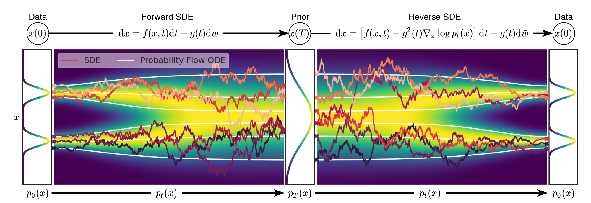
Perturbing data with multiple noise scales is key to the success of previous methods. We propose to generalize this idea further to an infinite number of noise scales, such that perturbed data distributions evolve according to an SDE as the noise intensifies. An overview of our framework is given in Figure 2.

3.1 Perturbing data with SDEs

Our goal is to construct a diffusion process ${\mathbf{x}(t)}{t=0}^T$ indexed by a continuous time variable $t\in [0, T]$, such that $\mathbf{x}(0) \sim p{0}$, for which we have a dataset of i.i.d samples, and $\mathbf{x}(T) \sim p_T$, for which we have a tractable form to generate samples efficiently. In other words, $p_0$ is the data distribution and $p_T$ is the prior distribution. This diffusion process can be modeled as the solution to an Itô SDE:

$ \begin{align} \mathrm{d} \mathbf{x} = \mathbf{f}(\mathbf{x}, t) \mathrm{d} t + {g}(t) \mathrm{d} \mathbf{w}, \end{align}\tag{5} $

where $\mathbf{w}$ is the standard Wiener process (a.k.a, Brownian motion), $\mathbf{f}(\cdot, t): \mathbb{R}^d \to \mathbb{R}^d$ is a vector-valued function called the drift coefficient of $\mathbf{x}(t)$, and ${g}(\cdot): \mathbb{R} \to \mathbb{R}$ is a scalar function known as the diffusion coefficient of $\mathbf{x}(t)$. For ease of presentation we assume the diffusion coefficient is a scalar (instead of a $d \times d$ matrix) and does not depend on $\mathbf{x}$, but our theory can be generalized to hold in those cases (see Appendix A). The SDE has a unique strong solution as long as the coefficients are globally Lipschitz in both state and time ([16]). We hereafter denote by $p_t(\mathbf{x})$ the probability density of $\mathbf{x}(t)$, and use $p_{st}(\mathbf{x}(t) \mid \mathbf{x}(s))$ to denote the transition kernel from $\mathbf{x}(s)$ to $\mathbf{x}(t)$, where $0 \leq s < t \leq T$.

Typically, $p_T$ is an unstructured prior distribution that contains no information of $p_0$, such as a Gaussian distribution with fixed mean and variance. There are various ways of designing the SDE in Equation 5 such that it diffuses the data distribution into a fixed prior distribution. We provide several examples later in Section 3.4 that are derived from continuous generalizations of SMLD and DDPM.

3.2 Generating samples by reversing the SDE

By starting from samples of $\mathbf{x}(T) \sim p_T$ and reversing the process, we can obtain samples $\mathbf{x}(0)\sim p_0$. A remarkable result from [12] states that the reverse of a diffusion process is also a diffusion process, running backwards in time and given by the reverse-time SDE:

$ \begin{align} \mathrm{d} \mathbf{x} = [\mathbf{f}(\mathbf{x}, t) - g(t)^2 \nabla_{\mathbf{x}} \log p_t(\mathbf{x})] \mathrm{d} t + g(t) \mathrm{d} \bar{\mathbf{w}}, \end{align}\tag{6} $

where $\bar{\mathbf{w}}$ is a standard Wiener process when time flows backwards from $T$ to $0$, and $\mathrm{d} t$ is an infinitesimal negative timestep. Once the score of each marginal distribution, $\nabla_\mathbf{x} \log p_t(\mathbf{x})$, is known for all $t$, we can derive the reverse diffusion process from Equation 6 and simulate it to sample from $p_0$.

3.3 Estimating scores for the SDE

The score of a distribution can be estimated by training a score-based model on samples with score matching ([17, 18]). To estimate $\nabla_\mathbf{x} \log p_t(\mathbf{x})$, we can train a time-dependent score-based model $\mathbf{s}_{\boldsymbol{\theta}}(\mathbf{x}, t)$ via a continuous generalization to 1 and 3:

$ \begin{align} {\boldsymbol{\theta}}^* = \operatorname{arg, min}{\boldsymbol{\theta}} \mathbb{E}{t}\Big{\lambda(t) \mathbb{E}{\mathbf{x}(0)}\mathbb{E}{\mathbf{x}(t) \mid \mathbf{x}(0) } \big[\left\lVert \mathbf{s}{\boldsymbol{\theta}}(\mathbf{x}(t), t) - \nabla{\mathbf{x}(t)}\log p_{0t}(\mathbf{x}(t) \mid \mathbf{x}(0))\right\rVert_2^2 \big]\Big} . \end{align}\tag{7} $

Here $\lambda: [0, T] \to \mathbb{R}{>0}$ is a positive weighting function, $t$ is uniformly sampled over $[0, T]$, $\mathbf{x}(0) \sim p_0(\mathbf{x})$ and $\mathbf{x}(t) \sim p{0t}(\mathbf{x}(t) \mid \mathbf{x}(0))$. With sufficient data and model capacity, score matching ensures that the optimal solution to 7, denoted by $\mathbf{s}{{\boldsymbol{\theta}}^\ast}(\mathbf{x}, t)$, equals $\nabla\mathbf{x} \log p_t(\mathbf{x})$ for almost all $\mathbf{x}$ and $t$. As in SMLD and DDPM, we can typically choose $\lambda \propto 1/{\mathbb{E}\big[\left\lVert\nabla_{\mathbf{x}(t)}\log p_{0t}(\mathbf{x}(t) \mid \mathbf{x}(0))\right\rVert_2^2\big]}$. Note that Equation 7 uses denoising score matching, but other score matching objectives, such as sliced score matching ([18]) and finite-difference score matching ([19]) are also applicable here.

We typically need to know the transition kernel $p_{0t}(\mathbf{x}(t) \mid \mathbf{x}(0))$ to efficiently solve Equation 7. When $\mathbf{f}(\cdot, t)$ is affine, the transition kernel is always a Gaussian distribution, where the mean and variance are often known in closed-forms and can be obtained with standard techniques (see Section 5.5 in [20]). For more general SDEs, we may solve Kolmogorov's forward equation ([16]) to obtain $p_{0t}(\mathbf{x}(t) \mid \mathbf{x}(0))$. Alternatively, we can simulate the SDE to sample from $p_{0t}(\mathbf{x}(t) \mid \mathbf{x}(0))$ and replace denoising score matching in Equation 7 with sliced score matching for model training, which bypasses the computation of $\nabla_{\mathbf{x}(t)} \log p_{0t}(\mathbf{x}(t) \mid \mathbf{x}(0))$ (see Appendix A).

3.4 Examples: VE, VP SDEs and beyond

The noise perturbations used in SMLD and DDPM can be regarded as discretizations of two different SDEs. Below we provide a brief discussion and relegate more details to Appendix B.

When using a total of $N$ noise scales, each perturbation kernel $p_{\sigma_i}(\mathbf{x} \mid \mathbf{x}_0)$ of SMLD corresponds to the distribution of $\mathbf{x}_i$ in the following Markov chain:

$ \begin{align} \mathbf{x}i = \mathbf{x}{i-1} + \sqrt{\sigma_{i}^2 - \sigma_{i-1}^2} \mathbf{z}_{i-1}, \quad i=1, \cdots, N, \end{align}\tag{8} $

where $\mathbf{z}{i-1} \sim \mathcal{N}(\mathbf{0}, \mathbf{I})$, and we have introduced $\sigma_0 = 0$ to simplify the notation. In the limit of $N \to \infty$, ${\sigma_i}{i=1}^N$ becomes a function $\sigma(t)$, $\mathbf{z}i$ becomes $\mathbf{z}(t)$, and the Markov chain ${\mathbf{x}i}{i=1}^N$ becomes a continuous stochastic process ${\mathbf{x}(t)}{t=0}^1$, where we have used a continuous time variable $t \in [0, 1]$ for indexing, rather than an integer $i$. The process ${\mathbf{x}(t)}_{t=0}^1$ is given by the following SDE

$ \begin{align} \mathrm{d} \mathbf{x} = \sqrt{\frac{\mathrm{d} \left[\sigma^2(t) \right]}{\mathrm{d} t}}\mathrm{d} \mathbf{w}. \end{align}\tag{9} $

Likewise for the perturbation kernels ${p_{\alpha_i}(\mathbf{x} \mid \mathbf{x}0)}{i=1}^N$ of DDPM, the discrete Markov chain is

$ \begin{align} \mathbf{x}i = \sqrt{1-\beta{i}} \mathbf{x}{i-1} + \sqrt{\beta{i}} \mathbf{z}_{i-1}, \quad i=1, \cdots, N. \end{align}\tag{10} $

As $N\to \infty$, Equation 10 converges to the following SDE,

$ \begin{align} \mathrm{d} \mathbf{x} = -\frac{1}{2}\beta(t) \mathbf{x}~ \mathrm{d} t + \sqrt{\beta(t)} ~ \mathrm{d} \mathbf{w}. \end{align}\tag{11} $

Therefore, the noise perturbations used in SMLD and DDPM correspond to discretizations of SDEs Equation 9 and 11. Interestingly, the SDE of Equation 9 always gives a process with exploding variance when $t \to \infty$, whilst the SDE of Equation 11 yields a process with a fixed variance of one when the initial distribution has unit variance (proof in Appendix B). Due to this difference, we hereafter refer to 9 as the Variance Exploding (VE) SDE, and 11 the Variance Preserving (VP) SDE.

Inspired by the VP SDE, we propose a new type of SDEs which perform particularly well on likelihoods (see Section 4.3), given by

$ \begin{align} \mathrm{d} \mathbf{x} = -\frac{1}{2}\beta(t) \mathbf{x}~ \mathrm{d} t + \sqrt{\beta(t)(1 - e^{-2\int_0^t \beta(s)\mathrm{d} s})} \mathrm{d} \mathbf{w}. \end{align}\tag{12} $

When using the same $\beta(t)$ and starting from the same initial distribution, the variance of the stochastic process induced by Equation 12 is always bounded by the VP SDE at every intermediate time step (proof in Appendix B). For this reason, we name Equation 12 the sub-VP SDE.

Since VE, VP and sub-VP SDEs all have affine drift coefficients, their perturbation kernels $p_{0t}(\mathbf{x}(t) \mid \mathbf{x}(0))$ are all Gaussian and can be computed in closed-forms, as discussed in Section 3.3. This makes training with Equation 7 particularly efficient.

4. Solving the reverse SDE

Section Summary: After training a score-based model, researchers use it to simulate a reverse-time stochastic differential equation (SDE) with numerical methods like Euler-Maruyama to generate new data samples from the original distribution. They introduce predictor-corrector samplers, which combine a basic SDE solver to predict sample positions with a refinement step using score estimates to correct and improve accuracy, outperforming simpler methods in experiments on image datasets. Additionally, the approach connects to a deterministic ordinary differential equation called the probability flow ODE, which shares the same data distribution as the SDE and enables exact likelihood calculations, akin to neural ODEs.

After training a time-dependent score-based model $\mathbf{s}_{\boldsymbol{\theta}}$, we can use it to construct the reverse-time SDE and then simulate it with numerical approaches to generate samples from $p_0$.

4.1 General-purpose numerical SDE solvers

Numerical solvers provide approximate trajectories from SDEs. Many general-purpose numerical methods exist for solving SDEs, such as Euler-Maruyama and stochastic Runge-Kutta methods ([21]), which correspond to different discretizations of the stochastic dynamics. We can apply any of them to the reverse-time SDE for sample generation.

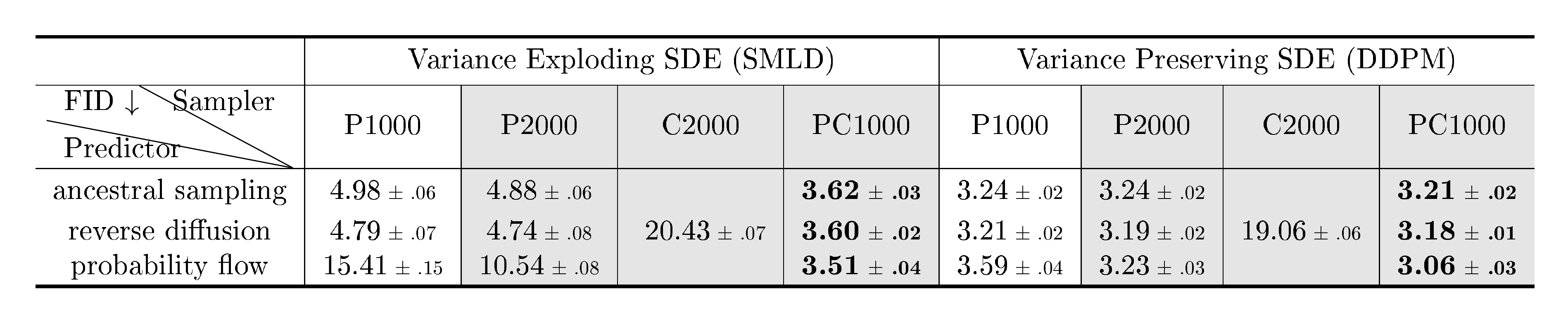
Ancestral sampling, the sampling method of DDPM Equation (4), actually corresponds to one special discretization of the reverse-time VP SDE Equation (11) (see Appendix E). Deriving the ancestral sampling rules for new SDEs, however, can be non-trivial. To remedy this, we propose reverse diffusion samplers (details in Appendix E), which discretize the reverse-time SDE in the same way as the forward one, and thus can be readily derived given the forward discretization. As shown in Table 1, reverse diffusion samplers perform slightly better than ancestral sampling for both SMLD and DDPM models on CIFAR-10 (DDPM-type ancestral sampling is also applicable to SMLD models, see Appendix F.)

4.2 Predictor-corrector samplers

Unlike generic SDEs, we have additional information that can be used to improve solutions. Since we have a score-based model $\mathbf{s}{{\boldsymbol{\theta}}^*}(\mathbf{x}, t) \approx \nabla\mathbf{x} \log p_t(\mathbf{x})$, we can employ score-based MCMC approaches, such as Langevin MCMC ([13, 22]) or HMC ([14]) to sample from $p_t$ directly, and correct the solution of a numerical SDE solver.

Specifically, at each time step, the numerical SDE solver first gives an estimate of the sample at the next time step, playing the role of a "predictor". Then, the score-based MCMC approach corrects the marginal distribution of the estimated sample, playing the role of a "corrector". The idea is analogous to Predictor-Corrector methods, a family of numerical continuation techniques for solving systems of equations ([23]), and we similarly name our hybrid sampling algorithms Predictor-Corrector (PC) samplers. Please find pseudo-code and a complete description in Appendix G. PC samplers generalize the original sampling methods of SMLD and DDPM: the former uses an identity function as the predictor and annealed Langevin dynamics as the corrector, while the latter uses ancestral sampling as the predictor and identity as the corrector.

::: {caption="Table 1: Comparing different reverse-time SDE solvers on CIFAR-10. Shaded regions are obtained with the same computation (number of score function evaluations). Mean and standard deviation are reported over five sampling runs. "P1000" or "P2000": predictor-only samplers using 1000 or 2000 steps. "C2000": corrector-only samplers using 2000 steps. "PC1000": Predictor-Corrector (PC) samplers using 1000 predictor and 1000 corrector steps."}

:::

We test PC samplers on SMLD and DDPM models (see Algorithm 2 and Algorithm 3 in Appendix G) trained with original discrete objectives given by Equation 1 and 3. This exhibits the compatibility of PC samplers to score-based models trained with a fixed number of noise scales. We summarize the performance of different samplers in Table 1, where probability flow is a predictor to be discussed in Section 4.3. Detailed experimental settings and additional results are given in Appendix G. We observe that our reverse diffusion sampler always outperform ancestral sampling, and corrector-only methods (C2000) perform worse than other competitors (P2000, PC1000) with the same computation (In fact, we need way more corrector steps per noise scale, and thus more computation, to match the performance of other samplers.) For all predictors, adding one corrector step for each predictor step (PC1000) doubles computation but always improves sample quality (against P1000). Moreover, it is typically better than doubling the number of predictor steps without adding a corrector (P2000), where we have to interpolate between noise scales in an ad hoc manner (detailed in Appendix G) for SMLD/DDPM models. In Figure 18 (Appendix G), we additionally provide qualitative comparison for models trained with the continuous objective Equation 7 on $256\times 256$ LSUN images and the VE SDE, where PC samplers clearly surpass predictor-only samplers under comparable computation, when using a proper number of corrector steps.

4.3 Probability flow and connection to neural ODEs

Score-based models enable another numerical method for solving the reverse-time SDE. For all diffusion processes, there exists a corresponding deterministic process whose trajectories share the same marginal probability densities ${p_t(\mathbf{x})}_{t=0}^T$ as the SDE. This deterministic process satisfies an ODE (more details in Appendix D.1):

$ \begin{align} \mathrm{d} \mathbf{x} = \Big[\mathbf{f}(\mathbf{x}, t) - \frac{1}{2} g(t)^2\nabla_\mathbf{x} \log p_t(\mathbf{x})\Big] \mathrm{d} t, \end{align}\tag{13} $

which can be determined from the SDE once scores are known. We name the ODE in Equation 13 the probability flow ODE. When the score function is approximated by the time-dependent score-based model, which is typically a neural network, this is an example of a neural ODE ([24]).

Exact likelihood computation Leveraging the connection to neural ODEs, we can compute the density defined by Equation 13 via the instantaneous change of variables formula ([24]). This allows us to compute the exact likelihood on any input data (details in Appendix D.2). As an example, we report negative log-likelihoods (NLLs) measured in bits/dim on the CIFAR-10 dataset in Table 2. We compute log-likelihoods on uniformly dequantized data, and only compare to models evaluated in the same way (omitting models evaluated with variational dequantization ([25]) or discrete data), except for DDPM ($L$ / $L_\text{simple}$) whose ELBO values (annotated with *) are reported on discrete data. Main results: (i) For the same DDPM model in [3], we obtain better bits/dim than ELBO, since our likelihoods are exact; (ii) Using the same architecture, we trained another DDPM model with the continuous objective in Equation 7 (i.e, DDPM cont.), which further improves the likelihood; (iii) With sub-VP SDEs, we always get higher likelihoods compared to VP SDEs; (iv) With improved architecture (i.e, DDPM++ cont., details in Section 4.4) and the sub-VP SDE, we can set a new record bits/dim of 2.99 on uniformly dequantized CIFAR-10 even without maximum likelihood training.

\begin{tabular}{l c c}
  \toprule
  Model & NLL Test $\downarrow$ & FID $\downarrow$ \\
  \midrule
  RealNVP ([26]) & 3.49 & -\\
  iResNet ([27]) & 3.45 & -\\
  Glow ([28]) & 3.35 & - \\
  MintNet ([29]) & 3.32 & - \\
  Residual Flow ([30]) & 3.28 & 46.37\\
  FFJORD ([31]) & 3.40 & -\\
  Flow++ ([25]) & 3.29 & -\\
  DDPM ($L$) ([3]) & $\leq$ 3.70\textsuperscript{*} & 13.51\\
  DDPM ($L_{\text{simple}}$) ([3]) & $\leq$ 3.75\textsuperscript{*} & 3.17\\
  \midrule
  DDPM & 3.28 & 3.37\\
  DDPM cont. (VP) & 3.21 & 3.69\\
  DDPM cont. (sub-VP) & 3.05 & 3.56\\
  DDPM++ cont. (VP) & 3.16 & 3.93\\
  DDPM++ cont. (sub-VP) & 3.02 & 3.16\\
  DDPM++ cont. (deep, VP) & 3.13 & 3.08\\
  DDPM++ cont. (deep, sub-VP) & \textbf{2.99} & \textbf{2.92} \\
  \bottomrule
  \end{tabular}

\begin{tabular}{lcc}
  \toprule
  Model & FID $\downarrow$ & IS $\uparrow$ \\
  \midrule
  {\bf Conditional} & & \\
  \midrule
  BigGAN ([32]) & 14.73 & 9.22 \\
  StyleGAN2-ADA ([33]) & \textbf{2.42} & \textbf{10.14} \\
  \midrule
  {\bf Unconditional} & & \\
  \midrule
  StyleGAN2-ADA ([33]) & 2.92 & 9.83 \\
  NCSN ([1]) & 25.32 & 8.87 $\pm$ .12 \\
  NCSNv2 ([7]) & 10.87 & 8.40 $\pm$ .07\\
  DDPM ([3]) & 3.17 & 9.46 $\pm$ .11\\
  \midrule
  DDPM++ & 2.78 & 9.64\\
  DDPM++ cont. (VP) & 2.55 & 9.58 \\
  DDPM++ cont. (sub-VP) & 2.61 & 9.56 \\
  DDPM++ cont. (deep, VP) & 2.41 & 9.68\\
  DDPM++ cont. (deep, sub-VP) & 2.41 & 9.57\\
  NCSN++ & 2.45 & 9.73 \\
  NCSN++ cont. (VE) & 2.38 & 9.83\\
  NCSN++ cont. (deep, VE) & \textbf{2.20} & \textbf{9.89}\\
  \bottomrule
  \end{tabular}

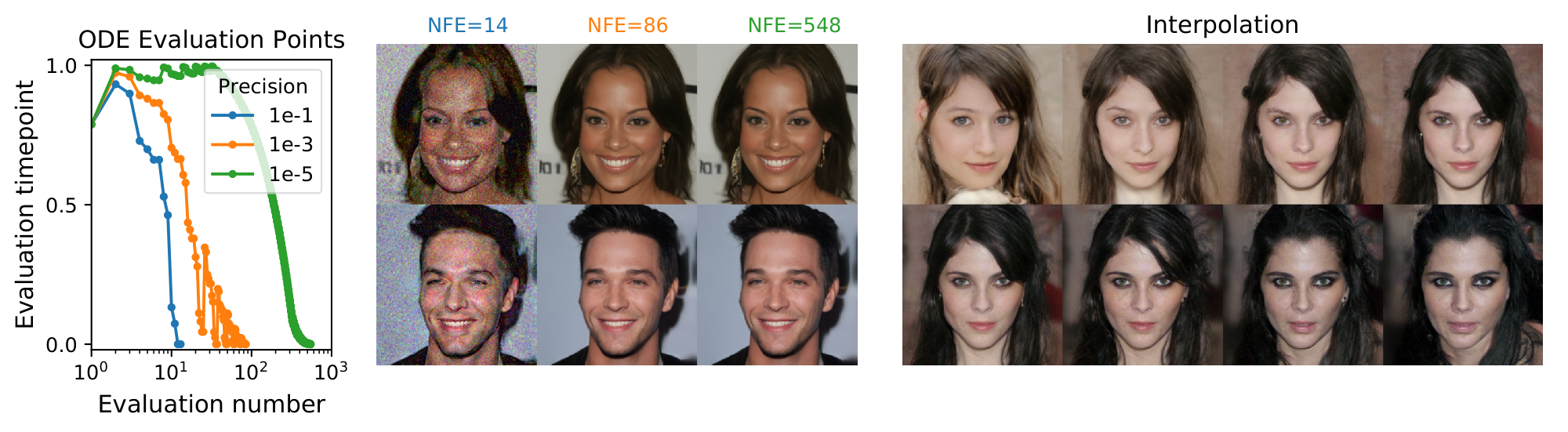
Manipulating latent representations By integrating Equation 13, we can encode any datapoint $\mathbf{x}(0)$ into a latent space $\mathbf{x}(T)$. Decoding can be achieved by integrating a corresponding ODE for the reverse-time SDE. As is done with other invertible models such as neural ODEs and normalizing flows ([26, 28]), we can manipulate this latent representation for image editing, such as interpolation, and temperature scaling (see Figure 3 and Appendix D.4).

Uniquely identifiable encoding Unlike most current invertible models, our encoding is uniquely identifiable, meaning that with sufficient training data, model capacity, and optimization accuracy, the encoding for an input is uniquely determined by the data distribution ([34]). This is because our forward SDE, Equation 5, has no trainable parameters, and its associated probability flow ODE, Equation 13, provides the same trajectories given perfectly estimated scores. We provide additional empirical verification on this property in Appendix D.5.

Efficient sampling As with neural ODEs, we can sample $\mathbf{x}(0) \sim p_0$ by solving Equation 13 from different final conditions $\mathbf{x}(T)\sim p_T$. Using a fixed discretization strategy we can generate competitive samples, especially when used in conjuction with correctors (Table 1, "probability flow sampler", details in Appendix D.3). Using a black-box ODE solver ([35]) not only produces high quality samples (Table 2, details in Appendix D.4), but also allows us to explicitly trade-off accuracy for efficiency. With a larger error tolerance, the number of function evaluations can be reduced by over $90%$ without affecting the visual quality of samples (Figure 3).

4.4 Architecture improvements

We explore several new architecture designs for score-based models using both VE and VP SDEs (details in Appendix H), where we train models with the same discrete objectives as in SMLD/DDPM. We directly transfer the architectures for VP SDEs to sub-VP SDEs due to their similarity. Our optimal architecture for the VE SDE, named NCSN++, achieves an FID of 2.45 on CIFAR-10 with PC samplers, while our optimal architecture for the VP SDE, called DDPM++, achieves 2.78.

By switching to the continuous training objective in Equation 7, and increasing the network depth, we can further improve sample quality for all models. The resulting architectures are denoted as NCSN++ cont. and DDPM++ cont. in Table 3 for VE and VP/sub-VP SDEs respectively. Results reported in Table 3 are for the checkpoint with the smallest FID over the course of training, where samples are generated with PC samplers. In contrast, FID scores and NLL values in Table 2 are reported for the last training checkpoint, and samples are obtained with black-box ODE solvers. As shown in Table 3, VE SDEs typically provide better sample quality than VP/sub-VP SDEs, but we also empirically observe that their likelihoods are worse than VP/sub-VP SDE counterparts. This indicates that practitioners likely need to experiment with different SDEs for varying domains and architectures.

Our best model for sample quality, NCSN++ cont. (deep, VE), doubles the network depth and sets new records for both inception score and FID on unconditional generation for CIFAR-10. Surprisingly, we can achieve better FID than the previous best conditional generative model without requiring labeled data. With all improvements together, we also obtain the first set of high-fidelity samples on CelebA-HQ $1024\times 1024$ from score-based models (see Appendix H.3). Our best model for likelihoods, DDPM++ cont. (deep, sub-VP), similarly doubles the network depth and achieves a log-likelihood of 2.99 bits/dim with the continuous objective in Equation 7. To our best knowledge, this is the highest likelihood on uniformly dequantized CIFAR-10.

5. Controllable generation

Section Summary: This section explains how the framework enables "controllable generation," where data samples can be produced not just from a basic probability distribution but also conditioned on specific observations, like labels or partial images, by reversing a noisy process with added guidance. This approach solves various inverse problems in generative modeling by estimating how observations relate to the noisy data at different stages, sometimes through trained models or simple heuristics. It demonstrates applications such as generating images for specific classes (like cars or horses from a dataset), filling in missing parts of an image (imputation), and adding color to grayscale versions, with examples shown in accompanying figures.

The continuous structure of our framework allows us to not only produce data samples from $p_0$, but also from $p_0(\mathbf{x}(0) \mid \mathbf{y})$ if $p_t(\mathbf{y} \mid \mathbf{x}(t))$ is known. Given a forward SDE as in Equation 5, we can sample from $p_t(\mathbf{x}(t) \mid \mathbf{y})$ by starting from $p_T(\mathbf{x}(T) \mid \mathbf{y})$ and solving a conditional reverse-time SDE:

$ \begin{align} \mathrm{d} \mathbf{x} = {\mathbf{f}(\mathbf{x}, t) - g(t)^2[\nabla_\mathbf{x} \log p_t(\mathbf{x})+ \nabla_{\mathbf{x}} \log p_t(\mathbf{y} \mid \mathbf{x})]} \mathrm{d} t + g(t) \mathrm{d} \bar{\mathbf{w}}. \end{align}\tag{14} $

In general, we can use Equation 14 to solve a large family of inverse problems with score-based generative models, once given an estimate of the gradient of the forward process, $\nabla_\mathbf{x} \log p_t(\mathbf{y} \mid \mathbf{x}(t))$. In some cases, it is possible to train a separate model to learn the forward process $\log p_t(\mathbf{y} \mid \mathbf{x}(t))$ and compute its gradient. Otherwise, we may estimate the gradient with heuristics and domain knowledge. In Appendix I.4, we provide a broadly applicable method for obtaining such an estimate without the need of training auxiliary models.

We consider three applications of controllable generation with this approach: class-conditional generation, image imputation and colorization. When $\mathbf{y}$ represents class labels, we can train a time-dependent classifier $p_t(\mathbf{y} \mid \mathbf{x}(t))$ for class-conditional sampling. Since the forward SDE is tractable, we can easily create training data $(\mathbf{x}(t), \mathbf{y})$ for the time-dependent classifier by first sampling $(\mathbf{x}(0), \mathbf{y})$ from a dataset, and then sampling $\mathbf{x}(t) \sim p_{0t}(\mathbf{x}(t) \mid \mathbf{x}(0))$. Afterwards, we may employ a mixture of cross-entropy losses over different time steps, like Equation 7, to train the time-dependent classifier $p_t(\mathbf{y} \mid \mathbf{x}(t))$. We provide class-conditional CIFAR-10 samples in Figure 4 (left), and relegate more details and results to Appendix I.

Imputation is a special case of conditional sampling. Suppose we have an incomplete data point $\mathbf{y}$ where only some subset, $\Omega(\mathbf{y})$ is known. Imputation amounts to sampling from $p(\mathbf{x}(0) \mid \Omega(\mathbf{y}))$, which we can accomplish using an unconditional model (see Appendix I.2). Colorization is a special case of imputation, except that the known data dimensions are coupled. We can decouple these data dimensions with an orthogonal linear transformation, and perform imputation in the transformed space (details in Appendix I.3). Figure 4 (right) shows results for inpainting and colorization achieved with unconditional time-dependent score-based models.

:::: {cols="1"}

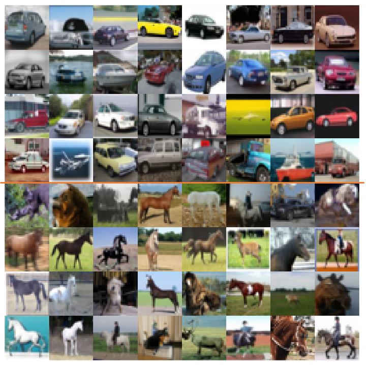
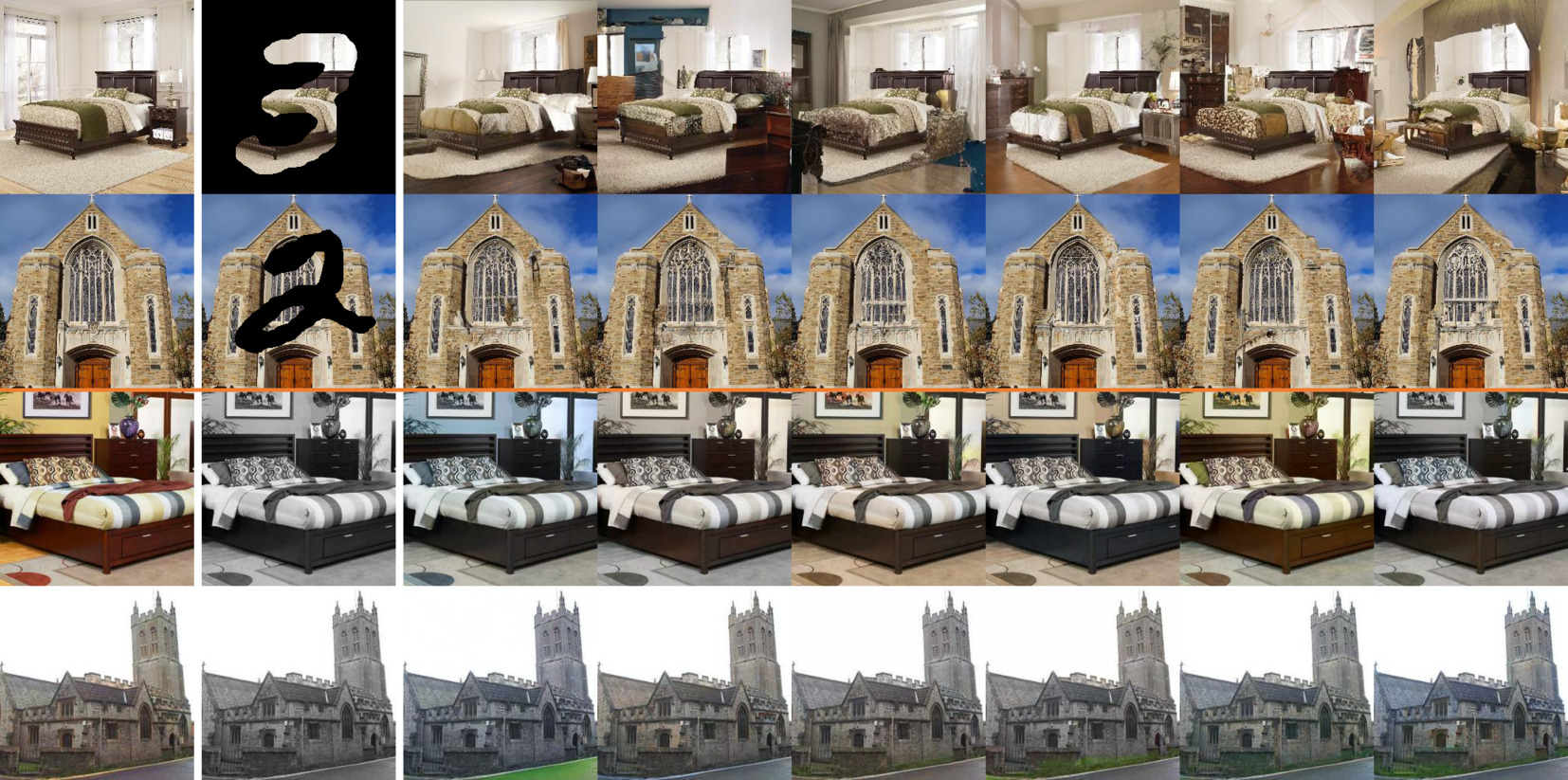
Figure 4: Left: Class-conditional samples on $32\times 32$ CIFAR-10. Top four rows are automobiles and bottom four rows are horses. Right: Inpainting (top two rows) and colorization (bottom two rows) results on $256\times 256$ LSUN. First column is the original image, second column is the masked/gray-scale image, remaining columns are sampled image completions or colorizations. ::::

6. Conclusion

Section Summary: This paper introduces a framework for score-based generative modeling using stochastic differential equations, which enhances understanding of current methods and enables innovations like new sampling techniques, precise likelihood calculations, unique data encoding, manipulation of hidden features, and conditional image generation. While the proposed sampling methods deliver improved results and efficiency over previous approaches, they are still slower than GANs, prompting future research to merge the reliable training of score-based models with the rapid generation of implicit models like GANs. Additionally, the variety of available samplers introduces many adjustable settings, so upcoming studies should focus on automating their selection and deeply exploring their strengths and weaknesses.

We presented a framework for score-based generative modeling based on SDEs. Our work enables a better understanding of existing approaches, new sampling algorithms, exact likelihood computation, uniquely identifiable encoding, latent code manipulation, and brings new conditional generation abilities to the family of score-based generative models.

While our proposed sampling approaches improve results and enable more efficient sampling, they remain slower at sampling than GANs ([36]) on the same datasets. Identifying ways of combining the stable learning of score-based generative models with the fast sampling of implicit models like GANs remains an important research direction. Additionally, the breadth of samplers one can use when given access to score functions introduces a number of hyper-parameters. Future work would benefit from improved methods to automatically select and tune these hyper-parameters, as well as more extensive investigation on the merits and limitations of various samplers.

Acknowledgements

We would like to thank Nanxin Chen, Ruiqi Gao, Jonathan Ho, Kevin Murphy, Tim Salimans and Han Zhang for their insightful discussions during the course of this project. This research was partially supported by NSF (#1651565, #1522054, #1733686), ONR (N00014-19-1-2145), AFOSR (FA9550-19-1-0024), and TensorFlow Research Cloud. Yang Song was partially supported by the Apple PhD Fellowship in AI/ML.

Appendix

Section Summary: The appendix section offers supplementary materials for the paper's framework on stochastic differential equations (SDEs) used in generative modeling, including detailed explanations and mathematical derivations. It starts with Appendix A, which extends the framework to handle more complex SDEs where the diffusion process depends on the data state, followed by appendices on deriving specific SDE types like variance-exploding, variance-preserving, and sub-variance-preserving models (B), practical guidance for using them (C), and formulations for probability flow ordinary differential equations along with sampling methods and likelihood computations (D). Additional sections cover various sampling techniques (E through G), model architectures with experimental details (H), and algorithms for controlled image generation tasks such as class conditioning, inpainting, colorization, and solving inverse problems (I).

We include several appendices with additional details, derivations, and results. Our framework allows general SDEs with matrix-valued diffusion coefficients that depend on the state, for which we provide a detailed discussion in Appendix A. We give a full derivation of VE, VP and sub-VP SDEs in Appendix B, and discuss how to use them from a practitioner's perspective in Appendix C. We elaborate on the probability flow formulation of our framework in Appendix D, including a derivation of the probability flow ODE (Appendix D.1), exact likelihood computation (Appendix D.2), probability flow sampling with a fixed discretization strategy (Appendix D.3), sampling with black-box ODE solvers (Appendix D.4), and experimental verification on uniquely identifiable encoding (Appendix D.5). We give a full description of the reverse diffusion sampler in Appendix E, the DDPM-type ancestral sampler for SMLD models in Appendix F, and Predictor-Corrector samplers in Appendix G. We explain our model architectures and detailed experimental settings in Appendix H, with $1024\times 1024$ CelebA-HQ samples therein. Finally, we detail on the algorithms for controllable generation in Appendix I, and include extended results for class-conditional generation (Appendix I.1), image inpainting (Appendix I.2), colorization (Appendix I.3), and a strategy for solving general inverse problems (Appendix I.4).

A. The framework for more general SDEs

In the main text, we introduced our framework based on a simplified SDE Equation 5 where the diffusion coefficient is independent of $\mathbf{x}(t)$. It turns out that our framework can be extended to hold for more general diffusion coefficients. We can consider SDEs in the following form:

$ \begin{align} \mathrm{d} \mathbf{x} = \mathbf{f}(\mathbf{x}, t) \mathrm{d} t + \mathbf{G}(\mathbf{x}, t) \mathrm{d} \mathbf{w}, \end{align}\tag{15} $

where $\mathbf{f}(\cdot, t): \mathbb{R}^d \to \mathbb{R}^d$ and $\mathbf{G}(\cdot, t): \mathbb{R}^d \to \mathbb{R}^{d\times d}$. We follow the Itô interpretation of SDEs throughout this paper.

According to ([12]), the reverse-time SDE is given by (cf, Equation 6)

$ \begin{align} \mathrm{d} \mathbf{x} = {\mathbf{f}(\mathbf{x}, t) - \nabla \cdot [\mathbf{G}(\mathbf{x}, t) \mathbf{G}(\mathbf{x}, t)^{\mkern-1.5mu\mathsf{T}}] - \mathbf{G}(\mathbf{x}, t)\mathbf{G}(\mathbf{x}, t)^{\mkern-1.5mu\mathsf{T}} \nabla_\mathbf{x} \log p_t(\mathbf{x})} \mathrm{d} t + \mathbf{G}(\mathbf{x}, t) \mathrm{d} \bar{\mathbf{w}}, \end{align}\tag{16} $

where we define $\nabla\cdot \mathbf{F}(\mathbf{x}) := (\nabla \cdot \mathbf{f}^1(\mathbf{x}), \nabla\cdot \mathbf{f}^2(\mathbf{x}), \cdots, \nabla\cdot \mathbf{f}^d(\mathbf{x}))^{\mkern-1.5mu\mathsf{T}}$ for a matrix-valued function $\mathbf{F}(\mathbf{x}) := (\mathbf{f}^1(\mathbf{x}), \mathbf{f}^2(\mathbf{x}), \cdots, \mathbf{f}^d(\mathbf{x}))^{\mkern-1.5mu\mathsf{T}}$ throughout the paper.

The probability flow ODE corresponding to 15 has the following form (cf, Equation 13, see a detailed derivation in Appendix D.1):

$ \begin{align} \mathrm{d} \mathbf{x} = \bigg{\mathbf{f}(\mathbf{x}, t) - \frac{1}{2} \nabla \cdot [\mathbf{G}(\mathbf{x}, t)\mathbf{G}(\mathbf{x}, t)^{\mkern-1.5mu\mathsf{T}}] - \frac{1}{2} \mathbf{G}(\mathbf{x}, t)\mathbf{G}(\mathbf{x}, t)^{\mkern-1.5mu\mathsf{T}} \nabla_\mathbf{x} \log p_t(\mathbf{x})\bigg} \mathrm{d} t. \end{align}\tag{17} $

Finally for conditional generation with the general SDE Equation 15, we can solve the conditional reverse-time SDE below (cf, Equation 14, details in Appendix I):

$ \begin{split} \mathrm{d} \mathbf{x} = {\mathbf{f}(\mathbf{x}, t) - \nabla \cdot [\mathbf{G}(\mathbf{x}, t) \mathbf{G}(\mathbf{x}, t)^{\mkern-1.5mu\mathsf{T}}] - \mathbf{G}(\mathbf{x}, t)\mathbf{G}(\mathbf{x}, t)^{\mkern-1.5mu\mathsf{T}} \nabla_\mathbf{x} \log p_t(\mathbf{x})\ - \mathbf{G}(\mathbf{x}, t)\mathbf{G}(\mathbf{x}, t)^{\mkern-1.5mu\mathsf{T}} \nabla_{\mathbf{x}} \log p_t(\mathbf{y} \mid \mathbf{x})} \mathrm{d} t + \mathbf{G}(\mathbf{x}, t) \mathrm{d} \bar{\mathbf{w}}. \end{split}\tag{18} $

When the drift and diffusion coefficient of an SDE are not affine, it can be difficult to compute the transition kernel $p_{0t}(\mathbf{x}(t) \mid \mathbf{x}(0))$ in closed form. This hinders the training of score-based models, because Equation 7 requires knowing $\nabla_{\mathbf{x}(t)}\log p_{0t}(\mathbf{x}(t) \mid \mathbf{x}(0))$. To overcome this difficulty, we can replace denoising score matching in Equation 7 with other efficient variants of score matching that do not require computing $\nabla_{\mathbf{x}(t)}\log p_{0t}(\mathbf{x}(t) \mid \mathbf{x}(0))$. For example, when using sliced score matching ([18]), our training objective Equation 7 becomes

$ \begin{align} {\boldsymbol{\theta}}^* = \operatorname{arg, min}{\boldsymbol{\theta}} \mathbb{E}{t}\bigg{\lambda(t) \mathbb{E}{\mathbf{x}(0)}\mathbb{E}{\mathbf{x}(t) }\mathbb{E}{\mathbf{v} \sim p\mathbf{v}} \bigg[\frac{1}{2}\left\lVert \mathbf{s}{\boldsymbol{\theta}}(\mathbf{x}(t), t)\right\rVert_2^2 + \mathbf{v} ^{\mkern-1.5mu\mathsf{T}} \mathbf{s}{\boldsymbol{\theta}}(\mathbf{x}(t), t) \mathbf{v} \bigg]\bigg} , \end{align}\tag{19} $

where $\lambda: [0, T] \to \mathbb{R}^+$ is a positive weighting function, $t \sim \mathcal{U}(0, T)$, $\mathbb{E}[\mathbf{v}] = \mathbf{0}$, and $\operatorname{Cov}[\mathbf{v}] = \mathbf{I}$. We can always simulate the SDE to sample from $p_{0t}(\mathbf{x}(t) \mid \mathbf{x}(0))$, and solve Equation 19 to train the time-dependent score-based model $\mathbf{s}_{\boldsymbol{\theta}}(\mathbf{x}, t)$.

B. VE, VP and sub-VP SDEs

Below we provide detailed derivations to show that the noise perturbations of SMLD and DDPM are discretizations of the Variance Exploding (VE) and Variance Preserving (VP) SDEs respectively. We additionally introduce sub-VP SDEs, a modification to VP SDEs that often achieves better performance in both sample quality and likelihoods.

First, when using a total of $N$ noise scales, each perturbation kernel $p_{\sigma_i}(\mathbf{x} \mid \mathbf{x}_0)$ of SMLD can be derived from the following Markov chain:

$ \begin{align} \mathbf{x}i = \mathbf{x}{i-1} + \sqrt{\sigma_{i}^2 - \sigma_{i-1}^2} \mathbf{z}_{i-1}, \quad i=1, \cdots, N, \end{align}\tag{8} $

where $\mathbf{z}{i-1} \sim \mathcal{N}(\mathbf{0}, \mathbf{I})$, $\mathbf{x}0 \sim p\text{data}$, and we have introduced $\sigma_0 = 0$ to simplify the notation. In the limit of $N \to \infty$, the Markov chain ${\mathbf{x}i}{i=1}^N$ becomes a continuous stochastic process ${\mathbf{x}(t)}{t=0}^1$, ${\sigma_i}_{i=1}^N$ becomes a function $\sigma(t)$, and $\mathbf{z}_i$ becomes $\mathbf{z}(t)$, where we have used a continuous time variable $t \in [0, 1]$ for indexing, rather than an integer $i \in {1, 2, \cdots, N}$. Let $\mathbf{x}\left(\frac{i}{N}\right) = \mathbf{x}_i$, $\sigma\left(\frac{i}{N}\right) = \sigma_i$, and $\mathbf{z}\left(\frac{i}{N}\right) = \mathbf{z}_i$ for $i=1, 2, \cdots, N$. We can rewrite Equation 8 as follows with $\Delta t = \frac{1}{N}$ and $t \in \big{0, \frac{1}{N}, \cdots, \frac{N-1}{N}\big}$:

$ \begin{align*} \mathbf{x}(t + \Delta t) = \mathbf{x}(t) + \sqrt{\sigma^2(t + \Delta t)- \sigma^2(t)}~ \mathbf{z}(t) \approx \mathbf{x}(t) + \sqrt{\frac{\mathrm{d} \left[\sigma^2(t) \right] }{\mathrm{d} t}\Delta t} ~ \mathbf{z}(t), \end{align*} $

where the approximate equality holds when $\Delta t \ll 1$. In the limit of $\Delta t \rightarrow 0$, this converges to

$ \begin{align} \mathrm{d} \mathbf{x} = \sqrt{\frac{\mathrm{d} \left[\sigma^2(t) \right]}{\mathrm{d} t}}\mathrm{d} \mathbf{w}, \end{align}\tag{20} $

which is the VE SDE.

For the perturbation kernels ${p_{\alpha_i}(\mathbf{x} \mid \mathbf{x}0)}{i=1}^N$ used in DDPM, the discrete Markov chain is

$ \begin{align} \mathbf{x}i = \sqrt{1-\beta{i}} \mathbf{x}{i-1} + \sqrt{\beta{i}} \mathbf{z}_{i-1}, \quad i=1, \cdots, N, \end{align}\tag{21} $

where $\mathbf{z}_{i-1} \sim \mathcal{N}(\mathbf{0}, \mathbf{I})$. To obtain the limit of this Markov chain when $N\to\infty$, we define an auxiliary set of noise scales ${\bar{\beta}i = N \beta_i}{i=1}^N$, and re-write Equation 21 as below

$ \begin{align} \mathbf{x}i = \sqrt{1-\frac{\bar{\beta}{i}}{N}} \mathbf{x}{i-1} + \sqrt{\frac{\bar{\beta}{i}}{N}} \mathbf{z}_{i-1}, \quad i=1, \cdots, N. \end{align}\tag{22} $

In the limit of $N\to \infty$, ${\bar{\beta}i}{i=1}^N$ becomes a function $\beta(t)$ indexed by $t \in [0, 1]$. Let $\beta\left(\frac{i}{N}\right) = \bar{\beta}_i$, $\mathbf{x}(\frac{i}{N}) = \mathbf{x}_i$, $\mathbf{z}(\frac{i}{N}) = \mathbf{z}_i$. We can rewrite the Markov chain Equation 22 as the following with $\Delta t = \frac{1}{N}$ and $t \in {0, 1, \cdots, \frac{N-1}{N}}$:

$ \begin{align} \mathbf{x}(t + \Delta t) &= \sqrt{1 - \beta(t + \Delta t)\Delta t} ~ \mathbf{x}(t) + \sqrt{\beta(t + \Delta t)\Delta t}~ \mathbf{z}(t) \notag\ &\approx \mathbf{x}(t) -\frac{1}{2}\beta(t + \Delta t)\Delta t~ \mathbf{x}(t) + \sqrt{\beta(t+\Delta t)\Delta t}~ \mathbf{z}(t) \notag\ &\approx \mathbf{x}(t) -\frac{1}{2}\beta(t)\Delta t~ \mathbf{x}(t) + \sqrt{\beta(t)\Delta t}~ \mathbf{z}(t), \end{align}\tag{23} $

where the approximate equality holds when $\Delta t \ll 1$. Therefore, in the limit of $\Delta t \to 0$, Equation 23 converges to the following VP SDE:

$ \begin{align} \mathrm{d} \mathbf{x} = -\frac{1}{2}\beta(t) \mathbf{x}~ \mathrm{d} t + \sqrt{\beta(t)} ~ \mathrm{d} \mathbf{w}. \end{align} $

So far, we have demonstrated that the noise perturbations used in SMLD and DDPM correspond to discretizations of VE and VP SDEs respectively. The VE SDE always yields a process with exploding variance when $t \to \infty$. In contrast, the VP SDE yields a process with bounded variance. In addition, the process has a constant unit variance for all $t \in [0, \infty)$ when $p(\mathbf{x}(0))$ has a unit variance. Since the VP SDE has affine drift and diffusion coefficients, we can use Eq. (5.51) in [20] to obtain an ODE that governs the evolution of variance

$ \begin{align*} \frac{\mathrm{d} \mathbf{\Sigma}\text{VP}(t)}{\mathrm{d} t} = \beta(t) (\mathbf{I} - \mathbf{\Sigma}\text{VP}(t)), \end{align*} $

where $\mathbf{\Sigma}\text{VP}(t) \coloneqq \operatorname{Cov}[\mathbf{x}(t)]$ for ${\mathbf{x}(t)}{t=0}^1$ obeying a VP SDE. Solving this ODE, we obtain

$ \begin{align} \mathbf{\Sigma}\text{VP}(t) = \mathbf{I} + e^{\int_0^t - \beta(s) \mathrm{d} s}(\mathbf{\Sigma}\text{VP}(0) - \mathbf{I}), \end{align} $

from which it is clear that the variance $\mathbf{\Sigma}\text{VP}(t)$ is always bounded given $\mathbf{\Sigma}\text{VP}(0)$. Moreover, $\mathbf{\Sigma}\text{VP}(t) \equiv \mathbf{I}$ if $\mathbf{\Sigma}\text{VP}(0) = \mathbf{I}$. Due to this difference, we name Equation 9 as the Variance Exploding (VE) SDE, and 11 the Variance Preserving (VP) SDE.

Inspired by the VP SDE, we propose a new SDE called the sub-VP SDE, namely

$ \begin{align} \mathrm{d} \mathbf{x} = -\frac{1}{2}\beta(t) \mathbf{x}~ \mathrm{d} t + \sqrt{\beta(t)(1 - e^{-2\int_0^t \beta(s)\mathrm{d} s})} \mathrm{d} \mathbf{w}. \end{align}\tag{24} $

Following standard derivations, it is straightforward to show that $\mathbb{E}[\mathbf{x}(t)]$ is the same for both VP and sub-VP SDEs; the variance function of sub-VP SDEs is different, given by

$ \begin{align} \mathbf{\Sigma}\text{sub-VP}(t) = \mathbf{I} + e^{-2 \int{0}^t \beta(s)\mathrm{d} s} \mathbf{I} + e^{-\int_0^t \beta(s) \mathrm{d} s}(\mathbf{\Sigma}_\text{sub-VP}(0) - 2 \mathbf{I}), \end{align} $

where $\mathbf{\Sigma}\text{sub-VP}(t) \coloneqq \operatorname{Cov}[\mathbf{x}(t)]$ for a process ${\mathbf{x}(t)}{t=0}^1$ obtained by solving Equation 24. In addition, we observe that (i) $\mathbf{\Sigma}{\text{sub-VP}}(t) \preccurlyeq \mathbf{\Sigma}{\text{VP}}(t)$ for all $t \geq 0$ with $\mathbf{\Sigma}\text{sub-VP}(0) = \mathbf{\Sigma}\text{VP}(0)$ and shared $\beta(s)$; and (ii) $\lim_{t\to \infty} \mathbf{\Sigma}{\text{sub-VP}}(t) = \lim{t \to \infty}\mathbf{\Sigma}{\text{VP}}(t) = \mathbf{I}$ if $\lim{t\to \infty}\int_0^t \beta(s) \mathrm{d} s = \infty$. The former is why we name Equation 24 the sub-VP SDE—its variance is always upper bounded by the corresponding VP SDE. The latter justifies the use of sub-VP SDEs for score-based generative modeling, since they can perturb any data distribution to standard Gaussian under suitable conditions, just like VP SDEs.

VE, VP and sub-VP SDEs all have affine drift coefficients. Therefore, their perturbation kernels $p_{0t}(\mathbf{x}(t) \mid \mathbf{x}(0))$ are all Gaussian and can be computed with Eqs. (5.50) and (5.51) in [20]:

$ \begin{align} p_{0t}(\mathbf{x}(t) \mid \mathbf{x}(0)) = \begin{cases} \mathcal{N}\big(\mathbf{x}(t) ; \mathbf{x}(0), [\sigma^2(t) - \sigma^2(0)] \mathbf{I}\big), &\quad \text{(VE SDE)}\ \mathcal{N}\big(\mathbf{x}(t) ; \mathbf{x}(0)e^{-\frac{1}{2}\int_0^t \beta(s) \mathrm{d} s}, \mathbf{I} - \mathbf{I} e^{-\int_0^t \beta(s) \mathrm{d} s}\big) &\quad \text{(VP SDE)}\ \mathcal{N}\big(\mathbf{x}(t) ; \mathbf{x}(0)e^{-\frac{1}{2}\int_0^t \beta(s) \mathrm{d} s}, [1 - e^{-\int_0^t \beta(s) \mathrm{d} s}]^2 \mathbf{I}\big) &\quad \text{(sub-VP SDE)} \end{cases}. \end{align}\tag{25} $

As a result, all SDEs introduced here can be efficiently trained with the objective in Equation 7.

C. SDEs in the wild

Below we discuss concrete instantiations of VE and VP SDEs whose discretizations yield SMLD and DDPM models, and the specific sub-VP SDE used in our experiments. In SMLD, the noise scales ${\sigma_i}{i=1}^N$ is typically a geometric sequence where $\sigma\text{min}$ is fixed to $0.01$ and $\sigma_\text{max}$ is chosen according to Technique 1 in [7]. Usually, SMLD models normalize image inputs to the range $[0, 1]$. Since ${\sigma_i}{i=1}^N$ is a geometric sequence, we have $\sigma(\frac{i}{N}) = \sigma_i = \sigma{\text{min}} \left(\frac{\sigma_{\text{max}}}{\sigma_{\text{min}}}\right)^{\frac{i-1}{N-1}}$ for $i=1, 2, \cdots, N$. In the limit of $N \to \infty$, we have $\sigma(t) = \sigma_{\text{min}} \left(\frac{\sigma_{\text{max}}}{\sigma_{\text{min}}}\right)^{t}$ for $t \in (0, 1]$. The corresponding VE SDE is

$ \begin{align} \mathrm{d} \mathbf{x} = \sigma_{\text{min}} \bigg(\frac{\sigma_{\text{max}}}{\sigma_{\text{min}}} \bigg)^t \sqrt{2 \log \frac{\sigma_{\text{max}}}{\sigma_{\text{min}}}}\mathrm{d} \mathbf{w}, \quad t \in (0, 1], \end{align} $

and the perturbation kernel can be derived via Equation 25:

$ \begin{align} p_{0t}(\mathbf{x}(t) \mid \mathbf{x}(0)) = \mathcal{N}\left(\mathbf{x}(t) ; \mathbf{x}(0), \sigma_{\text{min}}^2 \Big(\frac{\sigma_{\text{max}}}{\sigma_{\text{min}}}\Big)^{2t} \mathbf{I}\right), \quad t \in (0, 1]. \end{align} $

There is one subtlety when $t=0$: by definition, $\sigma(0) = \sigma_0 = 0$ (following the convention in Equation 8), but $\sigma(0^+) \coloneqq \lim_{t \to 0^+} \sigma(t) = \sigma_\text{min} \neq 0$. In other words, $\sigma(t)$ for SMLD is not differentiable since $\sigma(0) \neq \sigma(0^+)$, causing the VE SDE in Equation 20 undefined for $t=0$. In practice, we bypass this issue by always solving the SDE and its associated probability flow ODE in the range $t \in [\epsilon, 1]$ for some small constant $\epsilon > 0$, and we use $\epsilon = 10^{-5}$ in our VE SDE experiments.

For DDPM models, ${\beta_i}{i=1}^N$ is typically an arithmetic sequence where $\beta_i = \frac{\bar{\beta}{\text{min}}}{N} + \frac{i-1}{N(N-1)}(\bar{\beta}{\text{max}} - \bar{\beta}{\text{min}})$ for $i=1, 2, \cdots, N$. Therefore, $\beta(t) = \bar{\beta}{\text{min}} + t(\bar{\beta}{\text{max}} - \bar{\beta}_{\text{min}})$ for $t\in[0, 1]$ in the limit of $N \to \infty$. This corresponds to the following instantiation of the VP SDE:

$ \begin{gather} \mathrm{d} \mathbf{x} = -\frac{1}{2}(\bar{\beta}{\text{min}} + t(\bar{\beta}{\text{max}} - \bar{\beta}{\text{min}})) \mathbf{x} \mathrm{d} t + \sqrt{\bar{\beta}{\text{min}} + t(\bar{\beta}{\text{max}} - \bar{\beta}{\text{min}})} \mathrm{d} \mathbf{w}, \quad t\in[0, 1], \end{gather} $

where $\mathbf{x}(0) \sim p_\text{data}(\mathbf{x})$. In our experiments, we let $\bar{\beta}{\text{min}} = 0.1$ and $\bar{\beta}{\text{max}} = 20$ to match the settings in [3]. The perturbation kernel is given by

$ \begin{split} p_{0t}(\mathbf{x}(t) \mid \mathbf{x}(0)) \ = \mathcal{N}\left(\mathbf{x}(t) ; e^{-\frac{1}{4}t^2(\bar{\beta}{\text{max}}- \bar{\beta}{\text{min}}) - \frac{1}{2}t \bar{\beta}{\text{min}}}\mathbf{x}(0), \mathbf{I} - \mathbf{I} e^{-\frac{1}{2}t^2(\bar{\beta}{\text{max}} - \bar{\beta}{\text{min}}) - t \bar{\beta}{\text{min}}} \right), \quad t\in[0, 1]. \end{split} $

For DDPM, there is no discontinuity issue with the corresponding VP SDE; yet, there are numerical instability issues for training and sampling at $t=0$, due to the vanishing variance of $\mathbf{x}(t)$ as $t \to 0$. Therefore, same as the VE SDE, we restrict computation to $t\in[\epsilon, 1]$ for a small $\epsilon > 0$. For sampling, we choose $\epsilon=10^{-3}$ so that the variance of $\mathbf{x}(\epsilon)$ in VP SDE matches the variance of $\mathbf{x}_1$ in DDPM; for training and likelihood computation, we adopt $\epsilon=10^{-5}$ which empirically gives better results.

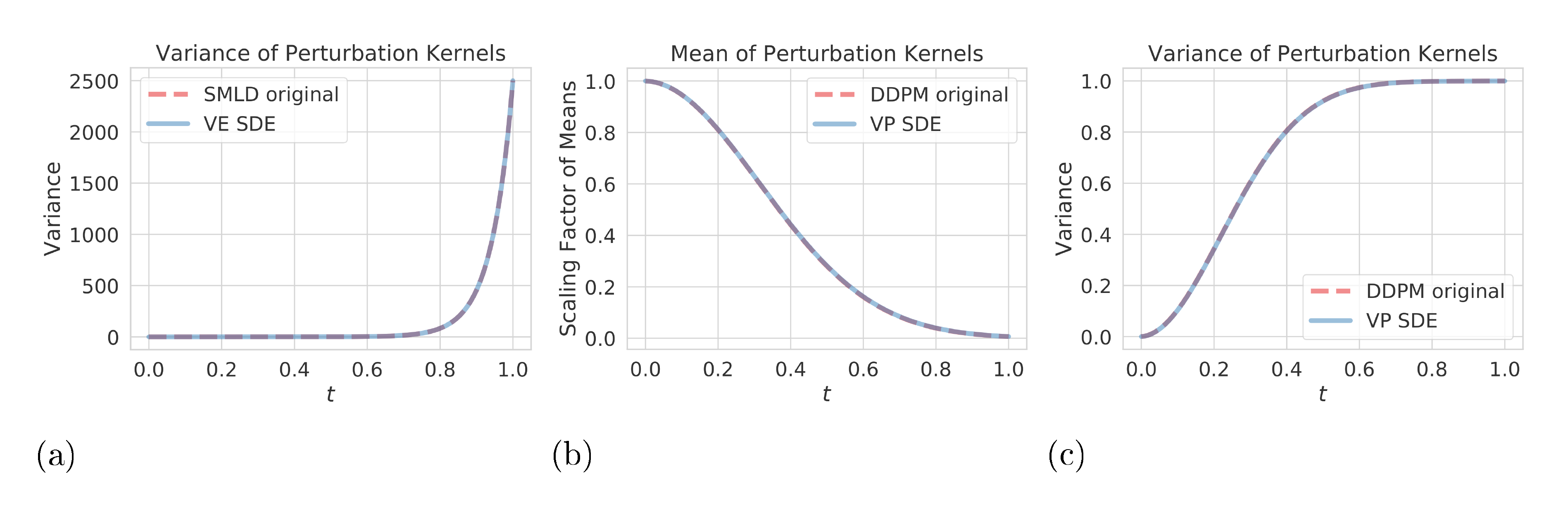
As a sanity check for our SDE generalizations to SMLD and DDPM, we compare the perturbation kernels of SDEs and original discrete Markov chains in Figure 8. The SMLD and DDPM models both use $N=1000$ noise scales. For SMLD, we only need to compare the variances of perturbation kernels since means are the same by definition. For DDPM, we compare the scaling factors of means and the variances. As demonstrated in Figure 8, the discrete perturbation kernels of original SMLD and DDPM models align well with perturbation kernels derived from VE and VP SDEs.

For sub-VP SDEs, we use exactly the same $\beta(t)$ as VP SDEs. This leads to the following perturbation kernel

$ \begin{split} p_{0t}(\mathbf{x}(t) \mid \mathbf{x}(0)) \ = \mathcal{N}\left(\mathbf{x}(t) ; e^{-\frac{1}{4}t^2(\bar{\beta}{\text{max}}- \bar{\beta}{\text{min}}) - \frac{1}{2}t \bar{\beta}{\text{min}}}\mathbf{x}(0), [1 - e^{-\frac{1}{2}t^2(\bar{\beta}{\text{max}} - \bar{\beta}{\text{min}}) - t \bar{\beta}{\text{min}}}]^2 \mathbf{I} \right), \quad t\in[0, 1]. \end{split} $

We also restrict numerical computation to the same interval of $[\epsilon, 1]$ as VP SDEs.

Empirically, we observe that smaller $\epsilon$ generally yields better likelihood values for all SDEs. For sampling, it is important to use an appropriate $\epsilon$ for better Inception scores and FIDs, although samples across different $\epsilon$ look visually the same to human eyes.

D. Probability flow ODE

D.1 Derivation

The idea of probability flow ODE is inspired by [37], and one can find the derivation of a simplified case therein. Below we provide a derivation for the fully general ODE in Equation 17. We consider the SDE in Equation 15, which possesses the following form:

$ \begin{align*} \mathrm{d} \mathbf{x} = \mathbf{f}(\mathbf{x}, t) \mathrm{d} t + \mathbf{G}(\mathbf{x}, t) \mathrm{d} \mathbf{w}, \end{align*} $

where $\mathbf{f}(\cdot, t): \mathbb{R}^d \to \mathbb{R}^d$ and $\mathbf{G}(\cdot, t): \mathbb{R}^d \to \mathbb{R}^{d\times d}$. The marginal probability density $p_t(\mathbf{x}(t))$ evolves according to Kolmogorov's forward equation (Fokker-Planck equation) ([16])

$ \begin{align} \frac{\partial p_t(\mathbf{x})}{\partial t} = -\sum_{i=1}^d \frac{\partial}{\partial x_i}[f_i(\mathbf{x}, t) p_t(\mathbf{x})] + \frac{1}{2}\sum_{i=1}^d\sum_{j=1}^d \frac{\partial^2}{\partial x_i \partial x_j}\Big[\sum_{k=1}^d G_{ik}(\mathbf{x}, t) G_{jk}(\mathbf{x}, t) p_t(\mathbf{x})\Big] . \end{align}\tag{26} $

We can easily rewrite Equation 26 to obtain

$ \begin{align} \frac{\partial p_t(\mathbf{x})}{\partial t} &= -\sum_{i=1}^d \frac{\partial}{\partial x_i}[f_i(\mathbf{x}, t) p_t(\mathbf{x})] + \frac{1}{2}\sum_{i=1}^d\sum_{j=1}^d \frac{\partial^2}{\partial x_i \partial x_j}\Big[\sum_{k=1}^d G_{ik}(\mathbf{x}, t) G_{jk}(\mathbf{x}, t) p_t(\mathbf{x})\Big]\notag \ &= -\sum_{i=1}^d \frac{\partial}{\partial x_i}[f_i(\mathbf{x}, t) p_t(\mathbf{x})] + \frac{1}{2}\sum_{i=1}^d \frac{\partial}{\partial x_i} \Big[\sum_{j=1}^d \frac{\partial}{\partial x_j}\Big[\sum_{k=1}^d G_{ik}(\mathbf{x}, t) G_{jk}(\mathbf{x}, t) p_t(\mathbf{x})\Big]\Big]. \end{align}\tag{27} $

Note that

$ \begin{align*} &\sum_{j=1}^d \frac{\partial}{\partial x_j}\Big[\sum_{k=1}^d G_{ik}(\mathbf{x}, t) G_{jk}(\mathbf{x}, t) p_t(\mathbf{x})\Big]\ =& \sum_{j=1}^d \frac{\partial}{\partial x_j} \Big[\sum_{k=1}^d G_{ik}(\mathbf{x}, t) G_{jk}(\mathbf{x}, t) \Big] p_t(\mathbf{x}) + \sum_{j=1}^d \sum_{k=1}^d G_{ik}(\mathbf{x}, t)G_{jk}(\mathbf{x}, t) p_t(\mathbf{x}) \frac{\partial}{\partial x_j} \log p_t(\mathbf{x})\ =& p_t(\mathbf{x}) \nabla \cdot [\mathbf{G}(\mathbf{x}, t)\mathbf{G}(\mathbf{x}, t)^{\mkern-1.5mu\mathsf{T}}] + p_t(\mathbf{x}) \mathbf{G}(\mathbf{x}, t)\mathbf{G}(\mathbf{x}, t)^{\mkern-1.5mu\mathsf{T}} \nabla_\mathbf{x} \log p_t(\mathbf{x}), \end{align*} $

based on which we can continue the rewriting of Equation 27 to obtain

$ \begin{align} \frac{\partial p_t(\mathbf{x})}{\partial t} &= -\sum_{i=1}^d \frac{\partial}{\partial x_i}[f_i(\mathbf{x}, t) p_t(\mathbf{x})] + \frac{1}{2}\sum_{i=1}^d \frac{\partial}{\partial x_i} \Big[\sum_{j=1}^d \frac{\partial}{\partial x_j}\Big[\sum_{k=1}^d G_{ik}(\mathbf{x}, t) G_{jk}(\mathbf{x}, t) p_t(\mathbf{x})\Big]\Big]\notag \ &= -\sum_{i=1}^d \frac{\partial}{\partial x_i}[f_i(\mathbf{x}, t) p_t(\mathbf{x})] \notag \ &\quad + \frac{1}{2}\sum_{i=1}^d \frac{\partial}{\partial x_i} \Big[p_t(\mathbf{x}) \nabla \cdot [\mathbf{G}(\mathbf{x}, t)\mathbf{G}(\mathbf{x}, t)^{\mkern-1.5mu\mathsf{T}}] + p_t(\mathbf{x}) \mathbf{G}(\mathbf{x}, t)\mathbf{G}(\mathbf{x}, t)^{\mkern-1.5mu\mathsf{T}} \nabla_\mathbf{x} \log p_t(\mathbf{x}) \Big]\notag \ &= -\sum_{i=1}^d \frac{\partial}{\partial x_i}\Big{ f_i(\mathbf{x}, t)p_t(\mathbf{x}) \notag \ &\quad - \frac{1}{2} \Big[\nabla \cdot [\mathbf{G}(\mathbf{x}, t)\mathbf{G}(\mathbf{x}, t)^{\mkern-1.5mu\mathsf{T}}] + \mathbf{G}(\mathbf{x}, t)\mathbf{G}(\mathbf{x}, t)^{\mkern-1.5mu\mathsf{T}} \nabla_\mathbf{x} \log p_t(\mathbf{x}) \Big] p_t(\mathbf{x}) \Big}\notag \ &= -\sum_{i=1}^d \frac{\partial}{\partial x_i} [\tilde{f}_i(\mathbf{x}, t)p_t(\mathbf{x})], \end{align}\tag{28} $

where we define

$ \begin{align*} \tilde{\mathbf{f}}(\mathbf{x}, t) \coloneqq \mathbf{f}(\mathbf{x}, t) - \frac{1}{2} \nabla \cdot [\mathbf{G}(\mathbf{x}, t)\mathbf{G}(\mathbf{x}, t)^{\mkern-1.5mu\mathsf{T}}] - \frac{1}{2} \mathbf{G}(\mathbf{x}, t)\mathbf{G}(\mathbf{x}, t)^{\mkern-1.5mu\mathsf{T}} \nabla_\mathbf{x} \log p_t(\mathbf{x}). \end{align*} $

Inspecting Equation 28, we observe that it equals Kolmogorov's forward equation of the following SDE with $\tilde{\mathbf{G}}(\mathbf{x}, t) \coloneqq \mathbf{0}$ (Kolmogorov's forward equation in this case is also known as the Liouville equation.)

$ \begin{align*} \mathrm{d} \mathbf{x} = \tilde{\mathbf{f}}(\mathbf{x}, t) \mathrm{d} t + \tilde{\mathbf{G}}(\mathbf{x}, t) \mathrm{d} \mathbf{w}, \end{align*} $

which is essentially an ODE:

$ \begin{align*} \mathrm{d} \mathbf{x} = \tilde{\mathbf{f}}(\mathbf{x}, t) \mathrm{d} t, \end{align*} $

same as the probability flow ODE given by Equation 17. Therefore, we have shown that the probability flow ODE Equation 17 induces the same marginal probability density $p_t(\mathbf{x})$ as the SDE in Equation 15.

D.2 Likelihood computation

The probability flow ODE in Equation 17 has the following form when we replace the score $\nabla_\mathbf{x} \log p_t(\mathbf{x})$ with the time-dependent score-based model $\mathbf{s}_{\boldsymbol{\theta}}(\mathbf{x}, t)$:

$ \begin{align} \mathrm{d} \mathbf{x} = \underbrace{\bigg{\mathbf{f}(\mathbf{x}, t) - \frac{1}{2} \nabla \cdot [\mathbf{G}(\mathbf{x}, t)\mathbf{G}(\mathbf{x}, t)^{\mkern-1.5mu\mathsf{T}}] - \frac{1}{2} \mathbf{G}(\mathbf{x}, t)\mathbf{G}(\mathbf{x}, t)^{\mkern-1.5mu\mathsf{T}} \mathbf{s}{\boldsymbol{\theta}}(\mathbf{x}, t)\bigg}}{=: \tilde{\mathbf{f}}_{\boldsymbol{\theta}}(\mathbf{x}, t)} \mathrm{d} t. \end{align}\tag{29} $

With the instantaneous change of variables formula ([24]), we can compute the log-likelihood of $p_0(\mathbf{x})$ using

$ \begin{align} \log p_0(\mathbf{x}(0)) = \log p_T(\mathbf{x}(T)) + \int_0^T \nabla \cdot \tilde{\mathbf{f}}_{\boldsymbol{\theta}}(\mathbf{x}(t), t) \mathrm{d} t, \end{align}\tag{30} $

where the random variable $\mathbf{x}(t)$ as a function of $t$ can be obtained by solving the probability flow ODE in Equation 29. In many cases computing $\nabla \cdot \tilde{\mathbf{f}}_{\boldsymbol{\theta}}(\mathbf{x}, t)$ is expensive, so we follow [31] to estimate it with the Skilling-Hutchinson trace estimator ([38, 39]). In particular, we have

$ \begin{align} \nabla \cdot \tilde{\mathbf{f}}{\boldsymbol{\theta}}(\mathbf{x}, t) = \mathbb{E}{p({\boldsymbol{\epsilon}})}[{\boldsymbol{\epsilon}} ^{\mkern-1.5mu\mathsf{T}} \nabla \tilde{\mathbf{f}}_{\boldsymbol{\theta}}(\mathbf{x}, t){\boldsymbol{\epsilon}}], \end{align}\tag{31} $

where $\nabla \tilde{\mathbf{f}}{\boldsymbol{\theta}}$ denotes the Jacobian of $\tilde{\mathbf{f}}{\boldsymbol{\theta}}(\cdot, t)$, and the random variable ${\boldsymbol{\epsilon}}$ satisfies $\mathbb{E}{p({\boldsymbol{\epsilon}})}[{\boldsymbol{\epsilon}}] = \mathbf{0}$ and $\operatorname{Cov}{p({\boldsymbol{\epsilon}})}[{\boldsymbol{\epsilon}}] = \mathbf{I}$. The vector-Jacobian product ${\boldsymbol{\epsilon}} ^{\mkern-1.5mu\mathsf{T}} \nabla\tilde{\mathbf{f}}{\boldsymbol{\theta}}(\mathbf{x}, t)$ can be efficiently computed using reverse-mode automatic differentiation, at approximately the same cost as evaluating $\tilde{\mathbf{f}}{\boldsymbol{\theta}}(\mathbf{x}, t)$. As a result, we can sample ${\boldsymbol{\epsilon}} \sim p({\boldsymbol{\epsilon}})$ and then compute an efficient unbiased estimate to $\nabla \cdot \tilde{\mathbf{f}}{\boldsymbol{\theta}}(\mathbf{x}, t)$ using ${\boldsymbol{\epsilon}} ^{\mkern-1.5mu\mathsf{T}} \nabla \tilde{\mathbf{f}}{\boldsymbol{\theta}}(\mathbf{x}, t) {\boldsymbol{\epsilon}}$. Since this estimator is unbiased, we can attain an arbitrarily small error by averaging over a sufficient number of runs. Therefore, by applying the Skilling-Hutchinson estimator Equation 31 to 30, we can compute the log-likelihood to any accuracy.

In our experiments, we use the RK45 ODE solver ([35]) provided by scipy.integrate.solve_ivp in all cases. The bits/dim values in Table 2 are computed with atol=1e-5 and rtol=1e-5, same as [31]. To give the likelihood results of our models in Table 2, we average the bits/dim obtained on the test dataset over five different runs with $\epsilon=10^{-5}$ (see definition of $\epsilon$ in Appendix C).

D.3 Probability flow sampling

Suppose we have a forward SDE

$ \begin{align*} \mathrm{d} \mathbf{x} = \mathbf{f}(\mathbf{x}, t) \mathrm{d} t + \mathbf{G}(t) \mathrm{d} \mathbf{w}, \end{align*} $

and one of its discretization

$ \begin{align} \mathbf{x}_{i+1} = \mathbf{x}_i + \mathbf{f}_i(\mathbf{x}_i) + \mathbf{G}_i \mathbf{z}_i, \quad i = 0, 1, \cdots, N-1, \end{align}\tag{32} $

where $\mathbf{z}_i \sim \mathcal{N}(\mathbf{0}, \mathbf{I})$. We assume the discretization schedule of time is fixed beforehand, and thus we absorb the dependency on $\Delta t$ into the notations of $\mathbf{f}_i$ and $\mathbf{G}_i$. Using Equation 17, we can obtain the following probability flow ODE:

$ \begin{align} \mathrm{d} \mathbf{x} = \left{ \mathbf{f}(\mathbf{x}, t) - \frac{1}{2}\mathbf{G}(t)\mathbf{G}(t)^{\mkern-1.5mu\mathsf{T}} \nabla_\mathbf{x} \log p_t(\mathbf{x}) \right} \mathrm{d} t. \end{align} $

We may employ any numerical method to integrate the probability flow ODE backwards in time for sample generation. In particular, we propose a discretization in a similar functional form to 32:

$ \begin{align*} \mathbf{x}i = \mathbf{x}{i+1} - \mathbf{f}{i+1}(\mathbf{x}{i+1}) + \frac{1}{2}\mathbf{G}{i+1}\mathbf{G}{i+1}^{\mkern-1.5mu\mathsf{T}} \mathbf{s}{{\boldsymbol{\theta}}^*}(\mathbf{x}{i+1}, i+1), \quad i =0, 1, \cdots, N-1, \end{align*} $

where the score-based model $\mathbf{s}_{{\boldsymbol{\theta}}^*}(\mathbf{x}_i, i)$ is conditioned on the iteration number $i$. This is a deterministic iteration rule. Unlike reverse diffusion samplers or ancestral sampling, there is no additional randomness once the initial sample $\mathbf{x}_N$ is obtained from the prior distribution. When applied to SMLD models, we can get the following iteration rule for probability flow sampling:

$ \begin{align} \mathbf{x}i = \mathbf{x}{i+1} + \frac{1}{2} (\sigma_{i+1}^2 - \sigma_i^2) \mathbf{s}{{{\boldsymbol{\theta}}^*}}(\mathbf{x}{i+1}, \sigma_{i+1}), \quad i=0, 1, \cdots, N-1. \end{align} $

Similarly, for DDPM models, we have

$ \begin{align} \mathbf{x}i = (2 - \sqrt{1 -\beta{i+1}})\mathbf{x}{i+1} + \frac{1}{2} \beta{i+1} \mathbf{s}{{\boldsymbol{\theta}}^*}(\mathbf{x}{i+1}, i+1), \quad i=0, 1, \cdots, N-1. \end{align} $

D.4 Sampling with black-box ODE solvers

For producing figures in Figure 3, we use a DDPM model trained on $256\times 256$ CelebA-HQ with the same settings in [3]. All FID scores of our models in Table 2 are computed on samples from the RK45 ODE solver implemented in scipy.integrate.solve_ivp with atol=1e-5 and rtol=1e-5. We use $\epsilon = 10^{-5}$ for VE SDEs and $\epsilon = 10^{-3}$ for VP SDEs (see also Appendix C).

Aside from the interpolation results in Figure 3, we demonstrate more examples of latent space manipulation in Figure 9, including interpolation and temperature scaling. The model tested here is a DDPM model trained with the same settings in [3].

:::: {cols="1"}

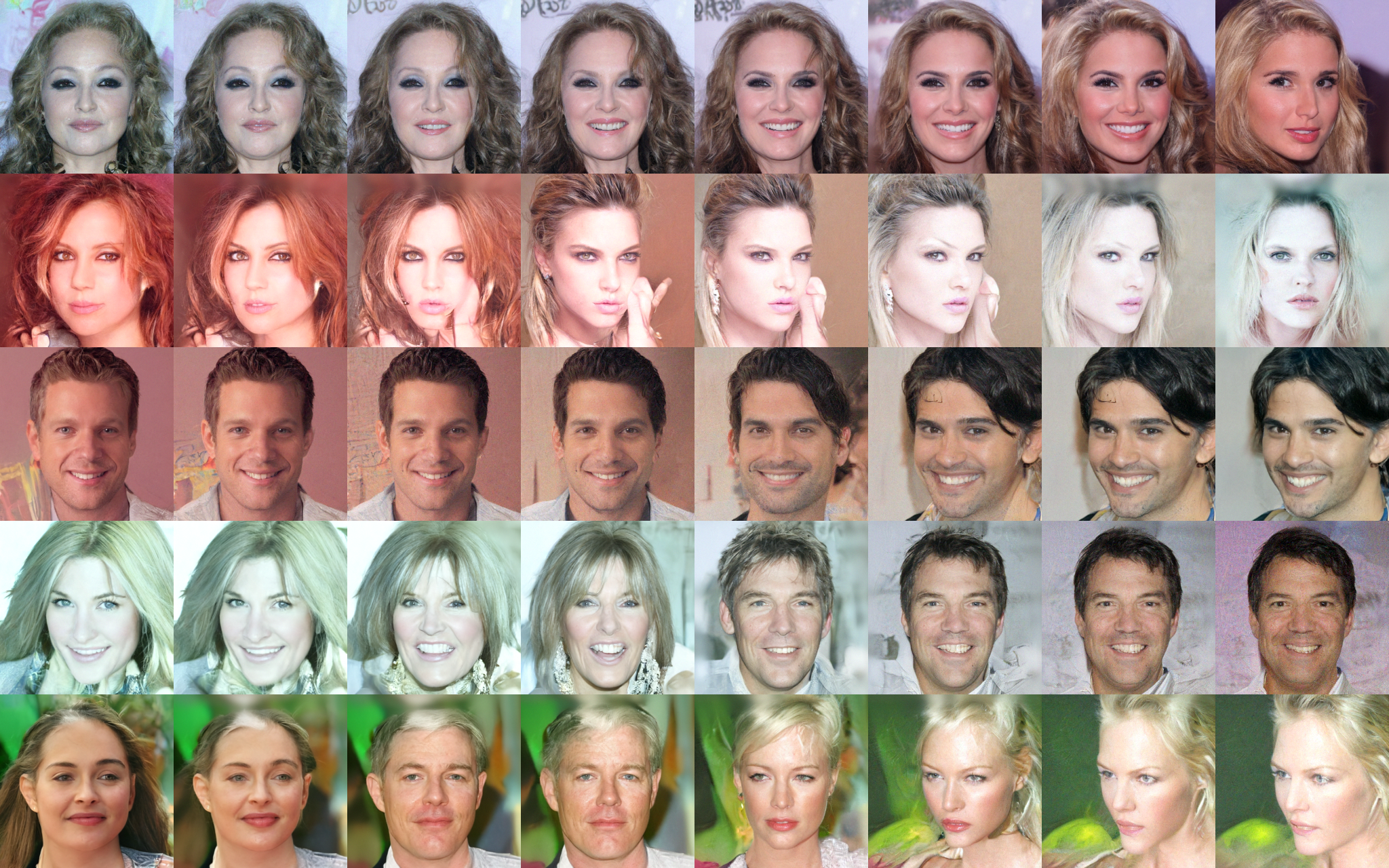
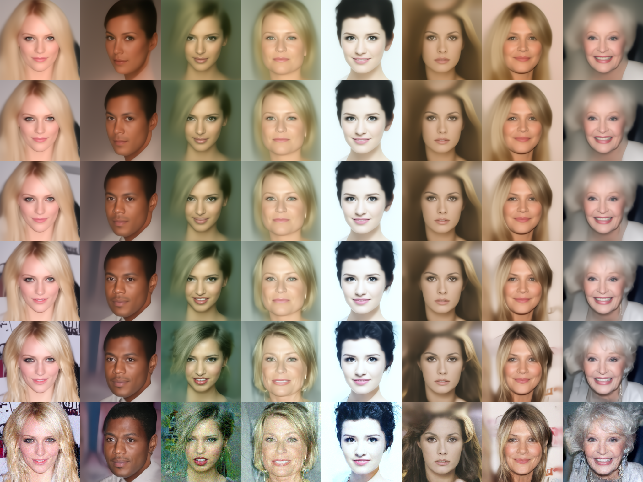
Figure 9: Samples from the probability flow ODE for VP SDE on $256\times 256$ CelebA-HQ. Top: spherical interpolations between random samples. Bottom: temperature rescaling (reducing norm of embedding). ::::

Although solvers for the probability flow ODE allow fast sampling, their samples typically have higher (worse) FID scores than those from SDE solvers if no corrector is used. We have this empirical observation for both the discretization strategy in Appendix D.3, and black-box ODE solvers introduced above. Moreover, the performance of probability flow ODE samplers depends on the choice of the SDE—their sample quality for VE SDEs is much worse than VP SDEs especially for high-dimensional data.

D.5 Uniquely identifiable encoding

:::: {cols="2"}

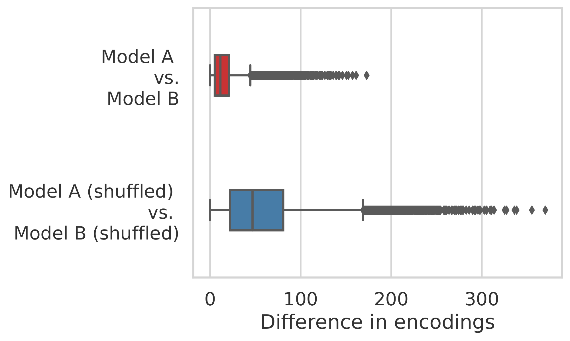
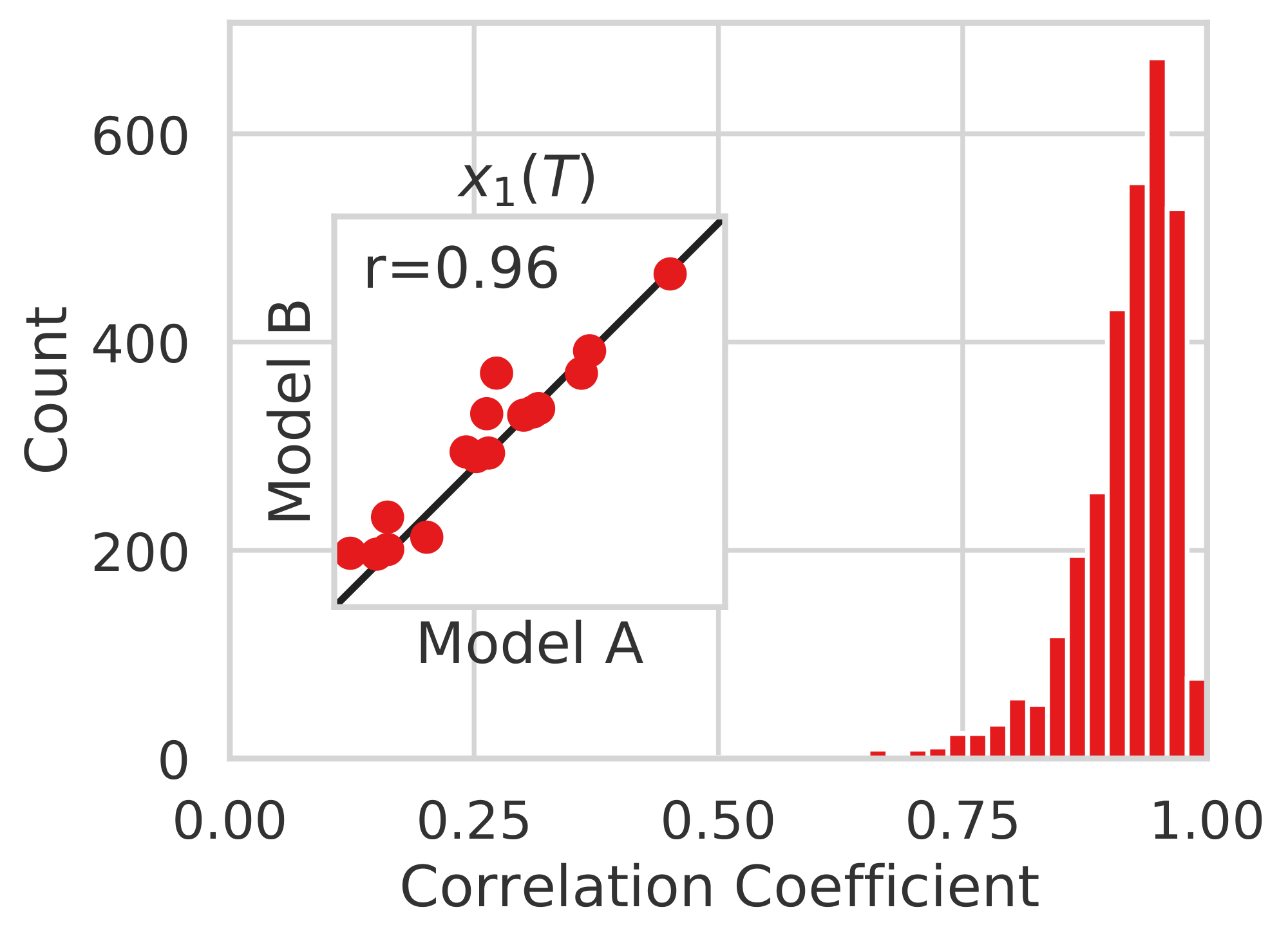
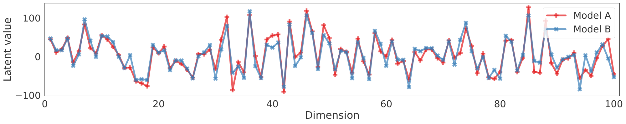
Figure 14: Left: The dimension-wise difference between encodings obtained by Model A and B. As a baseline, we also report the difference between shuffled representations of these two models. Right: The dimension-wise correlation coefficients of encodings obtained by Model A and Model B. ::::

As a sanity check, we train two models (denoted as "Model $A''$ and "Model $B'')$ with different architectures using the VE SDE on CIFAR-10. Here Model A is an NCSN++ model with 4 layers per resolution trained using the continuous objective in Equation 7, and Model B is all the same except that it uses 8 layers per resolution. Model definitions are in Appendix H.

We report the latent codes obtained by Model A and Model B for a random CIFAR-10 image in Figure 13. In Figure 14, we show the dimension-wise differences and correlation coefficients between latent encodings on a total of 16 CIFAR-10 images. Our results demonstrate that for the same inputs, Model A and Model B provide encodings that are close in every dimension, despite having different model architectures and training runs.

E. Reverse diffusion sampling

Given a forward SDE

$ \begin{align*} \mathrm{d} \mathbf{x} = \mathbf{f}(\mathbf{x}, t) \mathrm{d} t + \mathbf{G}(t) \mathrm{d} \mathbf{w}, \end{align*} $

and suppose the following iteration rule is a discretization of it:

$ \begin{align} \mathbf{x}_{i+1} = \mathbf{x}_i + \mathbf{f}_i(\mathbf{x}_i) + \mathbf{G}_i \mathbf{z}_i, \quad i = 0, 1, \cdots, N-1 \end{align}\tag{33} $

where $\mathbf{z}_i \sim \mathcal{N}(\mathbf{0}, \mathbf{I})$. Here we assume the discretization schedule of time is fixed beforehand, and thus we can absorb it into the notations of $\mathbf{f}_i$ and $\mathbf{G}_i$.

Based on Equation 33, we propose to discretize the reverse-time SDE

$ \begin{align*} \mathrm{d} \mathbf{x} = [\mathbf{f}(\mathbf{x}, t) - \mathbf{G}(t)\mathbf{G}(t)^{\mkern-1.5mu\mathsf{T}} \nabla_\mathbf{x} \log p_t(\mathbf{x})] \mathrm{d} t + \mathbf{G}(t) \mathrm{d} \bar{\mathbf{w}}, \end{align*} $

with a similar functional form, which gives the following iteration rule for $i \in {0, 1, \cdots, N-1}$:

$ \begin{align} \mathbf{x}{i} = \mathbf{x}{i+1} - \mathbf{f}{i+1}(\mathbf{x}{i+1}) + \mathbf{G}{i+1}\mathbf{G}{i+1}^{\mkern-1.5mu\mathsf{T}} \mathbf{s}{{\boldsymbol{\theta}}^*}(\mathbf{x}{i+1}, i+1) + \mathbf{G}{i+1}\mathbf{z}{i+1}, \end{align}\tag{34} $

where our trained score-based model $\mathbf{s}_{{\boldsymbol{\theta}}^*}(\mathbf{x}_i, i)$ is conditioned on iteration number $i$.

When applying Equation 34 to 8 and 10, we obtain a new set of numerical solvers for the reverse-time VE and VP SDEs, resulting in sampling algorithms as shown in the "predictor" part of Algorithm 2 and Algorithm 3. We name these sampling methods (that are based on the discretization strategy in Equation 34) reverse diffusion samplers.

As expected, the ancestral sampling of DDPM ([3]) Equation (4) matches its reverse diffusion counterpart when $\beta_i \to 0$ for all $i$ (which happens when $\Delta t \to 0$ since $\beta_i = \bar{\beta}_i \Delta t$, see Appendix B), because

$ \begin{align*} \mathbf{x}i = &\frac{1}{\sqrt{1-\beta{i+1}}}(\mathbf{x}{i+1} + \beta{i+1} \mathbf{s}{{\boldsymbol{\theta}}^*}(\mathbf{x}{i+1}, i+1)) + \sqrt{\beta_{i+1}} \mathbf{z}{i+1}\ =& \bigg(1 + \frac{1}{2}\beta{i+1} + o(\beta_{i+1}) \bigg)(\mathbf{x}{i+1} + \beta{i+1} \mathbf{s}{{\boldsymbol{\theta}}^*}(\mathbf{x}{i+1}, i+1)) + \sqrt{\beta_{i+1}} \mathbf{z}{i+1}\ \approx & \bigg(1 + \frac{1}{2}\beta{i+1} \bigg)(\mathbf{x}{i+1} + \beta{i+1} \mathbf{s}{{\boldsymbol{\theta}}^*}(\mathbf{x}{i+1}, i+1)) + \sqrt{\beta_{i+1}} \mathbf{z}{i+1}\ =&\bigg(1 + \frac{1}{2}\beta{i+1} \bigg) \mathbf{x}{i+1} + \beta{i+1}\mathbf{s}{{\boldsymbol{\theta}}^*}(\mathbf{x}{i+1}, i+1) + \frac{1}{2}\beta_{i+1}^2 \mathbf{s}{{\boldsymbol{\theta}}^*}(\mathbf{x}{i+1}, i+1) + \sqrt{\beta_{i+1}} \mathbf{z}{i+1}\ \approx& \bigg(1 + \frac{1}{2}\beta{i+1} \bigg) \mathbf{x}{i+1} + \beta{i+1}\mathbf{s}{{\boldsymbol{\theta}}^*}(\mathbf{x}{i+1}, i+1) + \sqrt{\beta_{i+1}} \mathbf{z}{i+1}\ =& \bigg[2 - \bigg(1 - \frac{1}{2}\beta{i+1}\bigg) \bigg] \mathbf{x}{i+1} + \beta{i+1}\mathbf{s}{{\boldsymbol{\theta}}^*}(\mathbf{x}{i+1}, i+1) + \sqrt{\beta_{i+1}} \mathbf{z}{i+1}\ \approx& \bigg[2 - \bigg(1 - \frac{1}{2}\beta{i+1}\bigg) + o(\beta_{i+1}) \bigg] \mathbf{x}{i+1} + \beta{i+1}\mathbf{s}{{\boldsymbol{\theta}}^*}(\mathbf{x}{i+1}, i+1) + \sqrt{\beta_{i+1}} \mathbf{z}{i+1}\ =& (2 - \sqrt{1-\beta{i+1}})\mathbf{x}{i+1} + \beta{i+1}\mathbf{s}{{\boldsymbol{\theta}}^*}(\mathbf{x}{i+1}, i+1)+ \sqrt{\beta_{i+1}} \mathbf{z}_{i+1}. \end{align*} $

Therefore, the original ancestral sampler of Equation 4 is essentially a different discretization to the same reverse-time SDE. This unifies the sampling method in [3] as a numerical solver to the reverse-time VP SDE in our continuous framework.

F. Ancestral sampling for SMLD models

The ancestral sampling method for DDPM models can also be adapted to SMLD models. Consider a sequence of noise scales $\sigma_1 < \sigma_2 < \cdots < \sigma_N$ as in SMLD. By perturbing a data point $\mathbf{x}_0$ with these noise scales sequentially, we obtain a Markov chain $\mathbf{x}_0 \to \mathbf{x}_1 \to \cdots \to \mathbf{x}_N$, where

$ \begin{align*} p(\mathbf{x}i \mid \mathbf{x}{i-1}) = \mathcal{N}(\mathbf{x}i; \mathbf{x}{i-1}, (\sigma_i^2 - \sigma_{i-1}^2)\mathbf{I}), \quad i=1, 2, \cdots, N. \end{align*} $

Here we assume $\sigma_0 = 0$ to simplify notations. Following [3], we can compute

$ \begin{align*} q(\mathbf{x}{i-1} \mid \mathbf{x}i, \mathbf{x}0) = \mathcal{N}\left(\mathbf{x}{i-1}; \frac{\sigma{i-1}^2}{\sigma{i}^2}\mathbf{x}i + \Big(1 - \frac{\sigma{i-1}^2}{\sigma_i^2} \Big)\mathbf{x}0, \frac{\sigma{i-1}^2 (\sigma_i^2 - \sigma_{i-1}^2)}{\sigma_i^2} \mathbf{I} \right). \end{align*} $

If we parameterize the reverse transition kernel as $p_{\boldsymbol{\theta}}(\mathbf{x}{i-1} \mid \mathbf{x}i) = \mathcal{N}(\mathbf{x}{i-1}; {\boldsymbol \mu}{\boldsymbol{\theta}}(\mathbf{x}_i, i), \tau^2_i \mathbf{I})$, then

$ \begin{align*} L_{t-1} &= \mathbb{E}q[D{\text{KL}}(q(\mathbf{x}_{i-1} \mid \mathbf{x}i, \mathbf{x}0))|p{\boldsymbol{\theta}}(\mathbf{x}{i-1} \mid \mathbf{x}i)]\ &= \mathbb{E}q\left[\frac{1}{2\tau^2_i} \left\lVert\frac{\sigma{i-1}^2}{\sigma{i}^2}\mathbf{x}i + \Big(1 - \frac{\sigma{i-1}^2}{\sigma_i^2} \Big)\mathbf{x}0 - {\boldsymbol \mu}{\boldsymbol{\theta}}(\mathbf{x}i, i)\right\rVert_2^2 \right] + C\ &=\mathbb{E}{\mathbf{x}_0, \mathbf{z}}\left[\frac{1}{2\tau^2_i} \left\lVert \mathbf{x}i(\mathbf{x}0, \mathbf{z}) - \frac{\sigma_i^2 - \sigma{i-1}^2}{\sigma_i} \mathbf{z} - {\boldsymbol \mu}{\boldsymbol{\theta}}(\mathbf{x}_i(\mathbf{x}_0, \mathbf{z}), i)\right\rVert_2^2 \right] + C, \end{align*} $

where $L_{t-1}$ is one representative term in the ELBO objective (see Eq. (8) in [3]), $C$ is a constant that does not depend on ${\boldsymbol{\theta}}$, $\mathbf{z} \sim \mathcal{N}(\mathbf{0}, \mathbf{I})$, and $\mathbf{x}_i(\mathbf{x}_0, \mathbf{z}) = \mathbf{x}0 + \sigma_i \mathbf{z}$. We can therefore parameterize ${\boldsymbol \mu}{\boldsymbol{\theta}}(\mathbf{x}_i, i)$ via

$ \begin{align*} {\boldsymbol \mu}_{\boldsymbol{\theta}}(\mathbf{x}i, i) = \mathbf{x}i + (\sigma_i^2 - \sigma{i-1}^2) \mathbf{s}{\boldsymbol{\theta}}(\mathbf{x}_i, i), \end{align*} $

where $\mathbf{s}{\boldsymbol{\theta}}(\mathbf{x}i, i)$ is to estimate $\mathbf{z} / \sigma_i$. As in [3], we let $\tau_i = \sqrt{\frac{\sigma{i-1}^2 (\sigma_i^2 - \sigma{i-1}^2)}{\sigma_i^2}}$. Through ancestral sampling on $\prod_{i=1}^N p_{\boldsymbol{\theta}}(\mathbf{x}_{i-1} \mid \mathbf{x}_i)$, we obtain the following iteration rule

$ \begin{align} \mathbf{x}{i-1} = \mathbf{x}i + (\sigma_i^2 - \sigma{i-1}^2) \mathbf{s}{{\boldsymbol{\theta}}^*}(\mathbf{x}i, i) + \sqrt{\frac{\sigma{i-1}^2 (\sigma_i^2 - \sigma_{i-1}^2)}{\sigma_i^2}} \mathbf{z}_i, i=1, 2, \cdots, N, \end{align}\tag{35} $

where $\mathbf{x}N \sim \mathcal{N}(\mathbf{0}, \sigma_N^2 \mathbf{I})$, ${\boldsymbol{\theta}}^*$ denotes the optimal parameter of $\mathbf{s}{\boldsymbol{\theta}}$, and $\mathbf{z}_i \sim \mathcal{N}(\mathbf{0}, \mathbf{I})$. We call Equation 35 the ancestral sampling method for SMLD models.

G. Predictor-Corrector samplers

**Require:**
$N$: Number of discretization steps for the reverse-time SDE
$M$: Number of corrector steps
Initialize $\mathbf{x}_N \sim p_T(\mathbf{x})$
**for** $i=N-1$ **to** $0$ **do**
  $\mathbf{x}_i \gets \operatorname{Predictor}(\mathbf{x}_{i+1})$
  **for** $j=1$ **to** $M$ **do**
    $\mathbf{x}_i \gets \operatorname{Corrector}(\mathbf{x}_i)$
  **end for**
**end for**
**return** $\mathbf{x}_0$

Predictor-Corrector (PC) sampling

The predictor can be any numerical solver for the reverse-time SDE with a fixed discretization strategy. The corrector can be any score-based MCMC approach. In PC sampling, we alternate between the predictor and corrector, as described in Algorithm 1. For example, when using the reverse diffusion SDE solver (Appendix E) as the predictor, and annealed Langevin dynamics ([1]) as the corrector, we have Algorithm 2 and Algorithm 3 for VE and VP SDEs respectively, where ${\epsilon_i}_{i=0}^{N-1}$ are step sizes for Langevin dynamics as specified below.

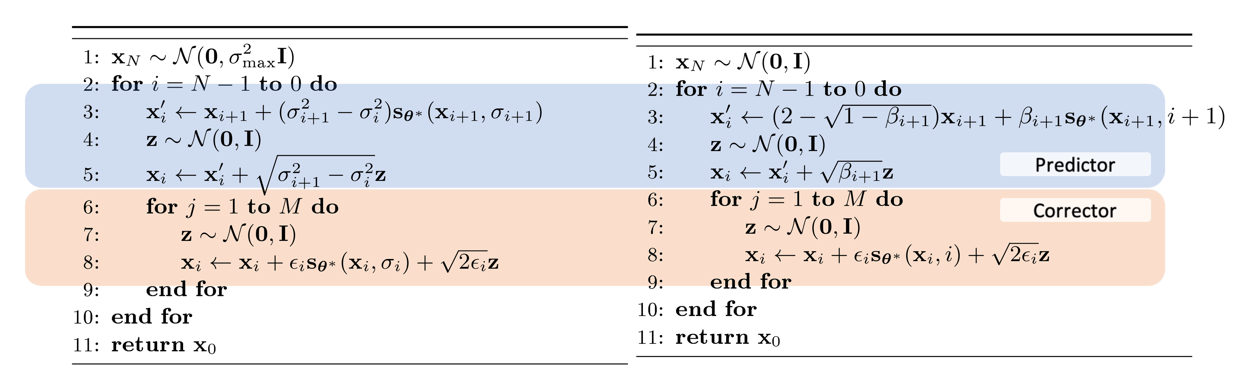
The corrector algorithms

We take the schedule of annealed Langevin dynamics in [1], but re-frame it with slight modifications in order to get better interpretability and empirical performance. We provide the corrector algorithms in Algorithm 4 and Algorithm 5 respectively, where we call $r$ the "signal-to-noise" ratio. We determine the step size $\epsilon$ using the norm of the Gaussian noise $\left\lVert \mathbf{z}\right\rVert_2$, norm of the score-based model $\left\lVert \mathbf{s}_{{\boldsymbol{\theta}}^*}\right\rVert_2$ and the signal-to-noise ratio $r$. When sampling a large batch of samples together, we replace the norm $\left\lVert\cdot\right\rVert_2$ with the average norm across the mini-batch. When the batch size is small, we suggest replacing $\left\lVert \mathbf{z}\right\rVert_2$ with $\sqrt{d}$, where $d$ is the dimensionality of $\mathbf{z}$.

**Require:** $\{\sigma_i\}_{i=1}^N, r, N, M$.
$\mathbf{x}_N^0 \sim \mathcal{N}(\mathbf{0}, \sigma_{\text{max}}^2 \mathbf{I})$
**for** $i \gets N$ to $1$ **do**
  **for** $j \gets 1$ to $M$ **do**
    $\mathbf{z} \sim \mathcal{N}(\mathbf{0}, \mathbf{I})$
    $\mathbf{g} \gets \mathbf{s}_{{\boldsymbol{\theta}}^*}(\mathbf{x}_i^j-1,\sigma_i)$
    $\epsilon \gets 2 (r \left\lVert \mathbf{z}\right\rVert_2 / \left\lVert \mathbf{g}\right\rVert_2)^2$
    $\mathbf{x}_i^j \gets \mathbf{x}_i^j-1 + \epsilon~ \mathbf{g}  + \sqrt{2 \epsilon}~ \mathbf{z}$
  **end for**
  $\mathbf{x}_i-1^0 \gets \mathbf{x}_i^M$
**end for**
**return** $\mathbf{x}_{0}^0$

**Require:** $\{\beta_i\}_{i=1}^N, \{\alpha_i\}_{i=1}^N, r, N, M$.
$\mathbf{x}_N^0 \sim \mathcal{N}(\mathbf{0}, \mathbf{I})$
**for** $i \gets N$ to $1$ **do**
  **for** $j \gets 1$ to $M$ **do**
    $\mathbf{z} \sim \mathcal{N}(\mathbf{0}, \mathbf{I})$
    $\mathbf{g} \gets \mathbf{s}_{{\boldsymbol{\theta}}^*}(\mathbf{x}_i^j-1, i)$
    $\epsilon \gets 2 \alpha_i (r \left\lVert \mathbf{z}\right\rVert_2 / \left\lVert \mathbf{g}\right\rVert_2)^2$
    $\mathbf{x}_i^j \gets \mathbf{x}_i^j-1 + \epsilon~ \mathbf{g}  + \sqrt{2 \epsilon}~ \mathbf{z}$
  **end for**
  $\mathbf{x}_i-1^0 \gets \mathbf{x}_i^M$
**end for**
**return** $\mathbf{x}_{0}^0$

Denoising

For both SMLD and DDPM models, the generated samples typically contain small noise that is hard to detect by humans. As noted by [40], FIDs can be significantly worse without removing this noise. This unfortunate sensitivity to noise is also part of the reason why NCSN models trained with SMLD has been performing worse than DDPM models in terms of FID, because the former does not use a denoising step at the end of sampling, while the latter does. In all experiments of this paper we ensure there is a single denoising step at the end of sampling, using Tweedie's formula ([41]).

:::: {cols="2"}

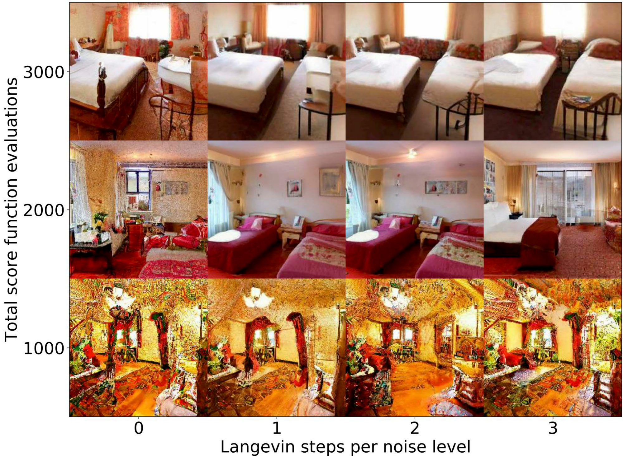
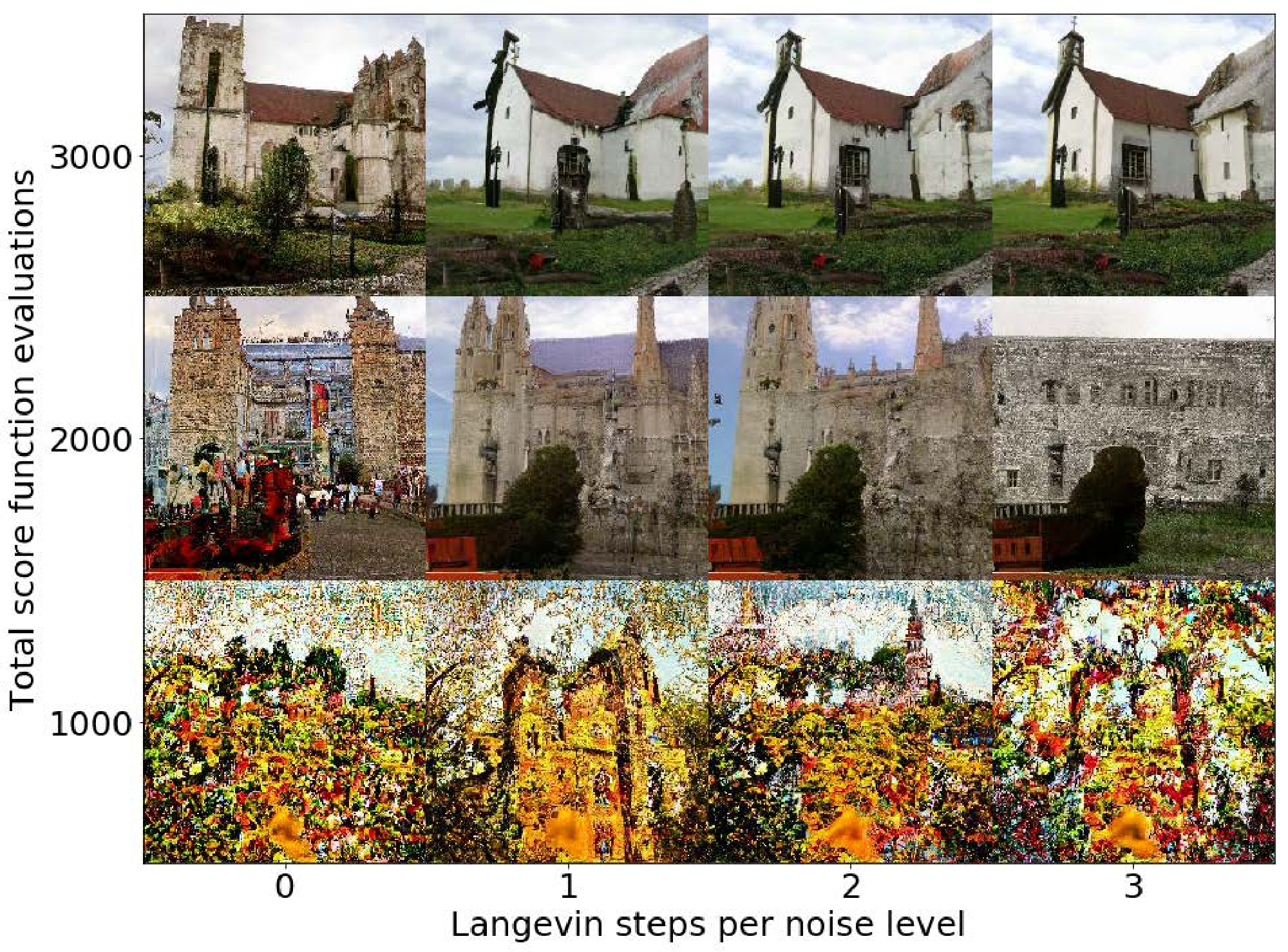
Figure 18: PC sampling for LSUN bedroom and church. The vertical axis corresponds to the total computation, and the horizontal axis represents the amount of computation allocated to the corrector. Samples are the best when computation is split between the predictor and corrector. ::::

Training

We use the same architecture in [3] for our score-based models. For the VE SDE, we train a model with the original SMLD objective in Equation 1; similarly for the VP SDE, we use the original DDPM objective in Equation 3. We apply a total number of 1000 noise scales for training both models. For results in Figure 18, we train an NCSN++ model (definition in Appendix H) on $256\times 256$ LSUN bedroom and church_outdoor ([42]) datasets with the VE SDE and our continuous objective Equation 7. The batch size is fixed to 128 on CIFAR-10 and 64 on LSUN.

Ad-hoc interpolation methods for noise scales

Models in this experiment are all trained with 1000 noise scales. To get results for P2000 (predictor-only sampler using 2000 steps) which requires 2000 noise scales, we need to interpolate between 1000 noise scales at test time. The specific architecture of the noise-conditional score-based model in [3] uses sinusoidal positional embeddings for conditioning on integer time steps. This allows us to interpolate between noise scales at test time in an ad-hoc way (while it is hard to do so for other architectures like the one in [1]). Specifically, for SMLD models, we keep $\sigma_{\text{min}}$ and $\sigma_{\text{max}}$ fixed and double the number of time steps. For DDPM models, we halve $\beta_{\text{min}}$ and $\beta_{\text{max}}$ before doubling the number of time steps. Suppose ${\mathbf{s}{\boldsymbol{\theta}}(\mathbf{x}, i)}{i=0}^{N-1}$ is a score-based model trained on $N$ time steps, and let ${\mathbf{s}{\boldsymbol{\theta}}'(\mathbf{x}, i)}{i=0}^{2N-1}$ denote the corresponding interpolated score-based model at $2N$ time steps. We test two different interpolation strategies for time steps: linear interpolation where $\mathbf{s}{\boldsymbol{\theta}}'(\mathbf{x}, i) = \mathbf{s}{\boldsymbol{\theta}}(\mathbf{x}, i / 2)$ and rounding interpolation where $\mathbf{s}{\boldsymbol{\theta}}'(\mathbf{x}, i) = \mathbf{s}{\boldsymbol{\theta}}(\mathbf{x}, \lfloor i/2 \rfloor)$. We provide results with linear interpolation in Table 1, and give results of rounding interpolation in Table 4. We observe that different interpolation methods result in performance differences but maintain the general trend of predictor-corrector methods performing on par or better than predictor-only or corrector-only samplers.

Hyper-parameters of the samplers

For Predictor-Corrector and corrector-only samplers on CIFAR-10, we search for the best signal-to-noise ratio ($r$) over a grid that increments at 0.01. We report the best $r$ in Table 5. For LSUN bedroom/church_outdoor, we fix $r$ to 0.075. Unless otherwise noted, we use one corrector step per noise scale for all PC samplers. We use two corrector steps per noise scale for corrector-only samplers on CIFAR-10. For sample generation, the batch size is 1024 on CIFAR-10 and 8 on LSUN bedroom/church_outdoor.

::: {caption="Table 4: Comparing different samplers on CIFAR-10, where "P2000" uses the rounding interpolation between noise scales. Shaded regions are obtained with the same computation (number of score function evaluations). Mean and standard deviation are reported over five sampling runs."}

:::

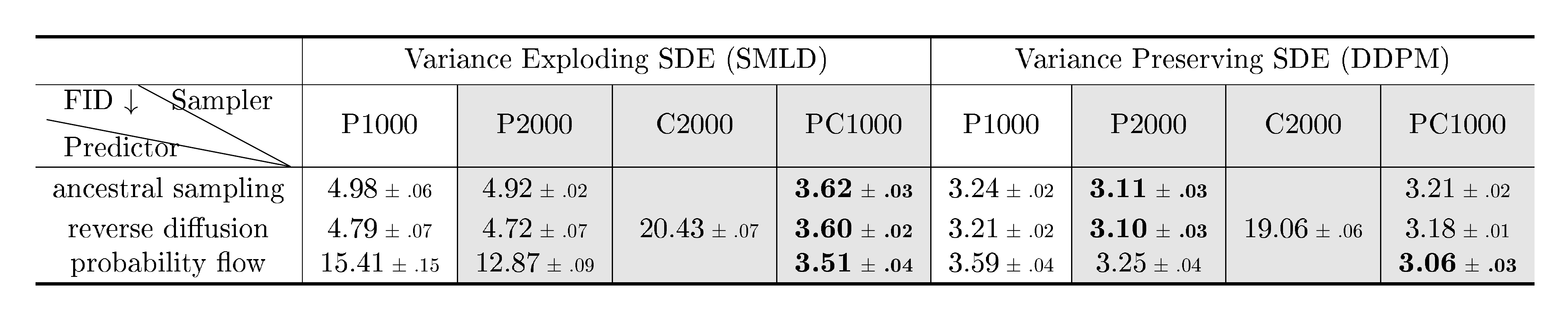
::: {caption="Table 5: Optimal signal-to-noise ratios of different samplers. "P1000" or "P2000": predictor-only samplers using 1000 or 2000 steps. "C2000": corrector-only samplers using 2000 steps. "PC1000": PC samplers using 1000 predictor and 1000 corrector steps."}

:::

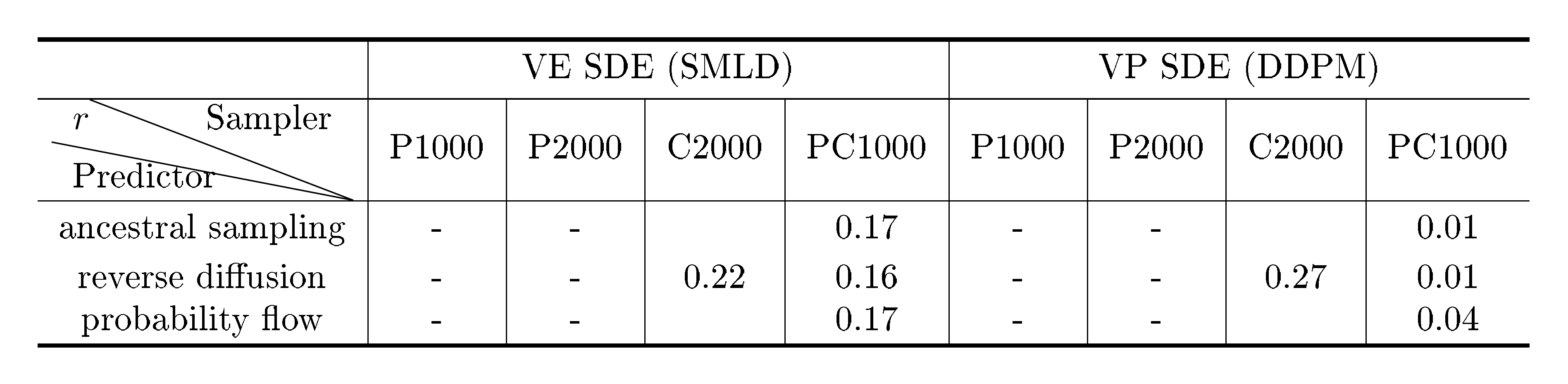
H. Architecture improvements

We explored several architecture designs to improve score-based models for both VE and VP SDEs. Our endeavor gives rise to new state-of-the-art sample quality on CIFAR-10, new state-of-the-art likelihood on uniformly dequantized CIFAR-10, and enables the first high-fidelity image samples of resolution $1024\times 1024$ from score-based generative models. Code and checkpoints are open-sourced at https://github.com/yang-song/score_sde.

H.1 Settings for architecture exploration

Unless otherwise noted, all models are trained for 1.3M iterations, and we save one checkpoint per 50k iterations. For VE SDEs, we consider two datasets: $32\times 32$ CIFAR-10 ([43]) and $64\times 64$ CelebA ([44]), pre-processed following [7]. We compare different configurations based on their FID scores averaged over checkpoints after 0.5M iterations. For VP SDEs, we only consider the CIFAR-10 dataset to save computation, and compare models based on the average FID scores over checkpoints obtained between 0.25M and 0.5M iterations, because FIDs turn to increase after 0.5M iterations for VP SDEs.

All FIDs are computed on 50k samples with . For sampling, we use the PC sampler discretized at 1000 time steps. We choose reverse diffusion (see Appendix E) as the predictor. We use one corrector step per update of the predictor for VE SDEs with a signal-to-noise ratio of 0.16, but save the corrector step for VP SDEs since correctors there only give slightly better results but require double computation. We follow [3] for optimization, including the learning rate, gradient clipping, and learning rate warm-up schedules. Unless otherwise noted, models are trained with the original discrete SMLD and DDPM objectives in Equation 1 and 3 and use a batch size of 128. The optimal architectures found under these settings are subsequently transferred to continuous objectives and deeper models. We also directly transfer the best architecture for VP SDEs to sub-VP SDEs, given the similarity of these two SDEs.

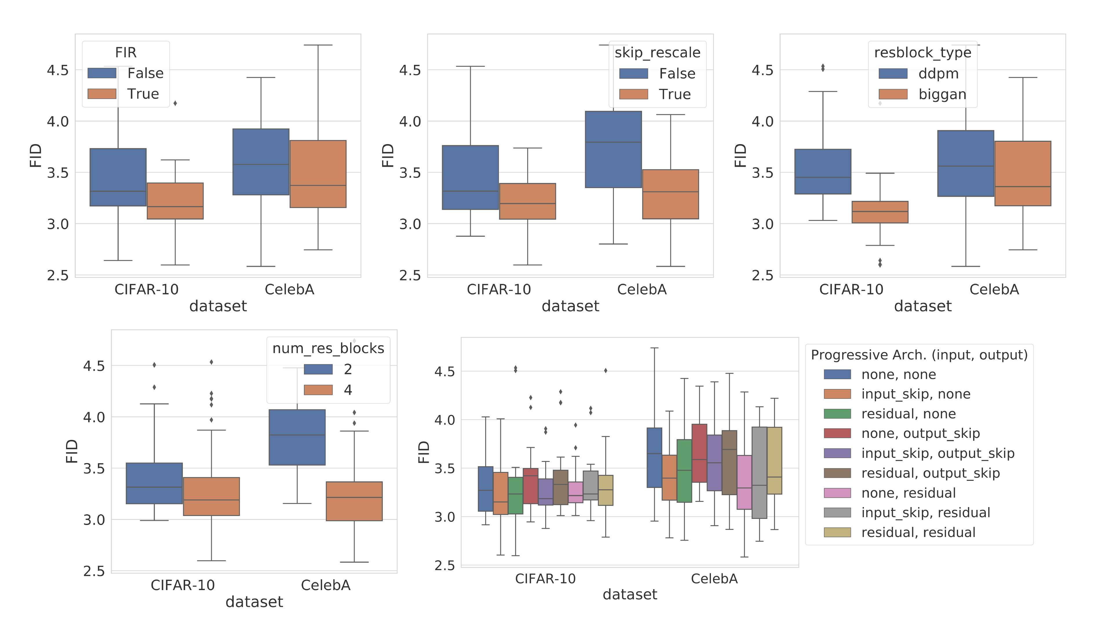
Our architecture is mostly based on [3]. We additionally introduce the following components to maximize the potential improvement of score-based models.

1. Upsampling and downsampling images with anti-aliasing based on Finite Impulse Response (FIR) ([45]). We follow the same implementation and hyper-parameters in StyleGAN-2 ([46]).
2. Rescaling all skip connections by $\frac{1}{\sqrt{2}}$. This has been demonstrated effective in several best-in-class GAN models, including ProgressiveGAN ([47]), StyleGAN ([48]) and StyleGAN-2 ([46]).
3. Replacing the original residual blocks in DDPM with residual blocks from BigGAN ([32]).
4. Increasing the number of residual blocks per resolution from $2$ to $4$.
5. Incorporating progressive growing architectures. We consider two progressive architectures for input: "input skip" and "residual", and two progressive architectures for output: "output skip" and "residual". These progressive architectures are defined and implemented according to StyleGAN-2.

We also tested equalized learning rates, a trick used in very successful models like ProgressiveGAN ([47]) and StyleGAN ([48]). However, we found it harmful at an early stage of our experiments, and therefore decided not to explore more on it.

The exponential moving average (EMA) rate has a significant impact on performance. For models trained with VE perturbations, we notice that 0.999 works better than 0.9999, whereas for models trained with VP perturbations it is the opposite. We therefore use an EMA rate of 0.999 and 0.9999 for VE and VP models respectively.

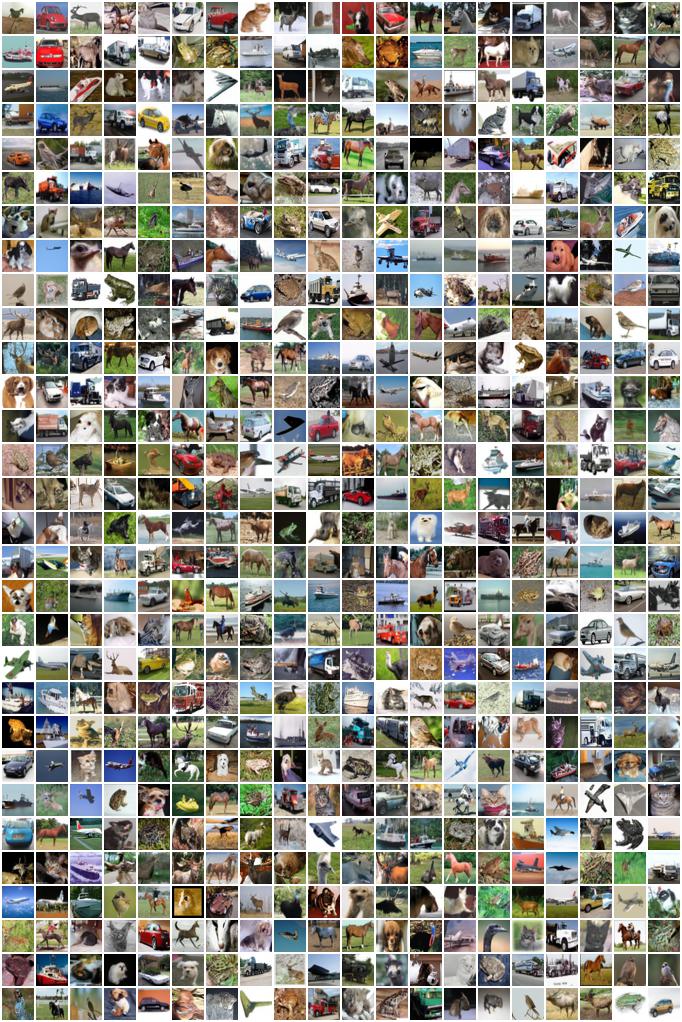
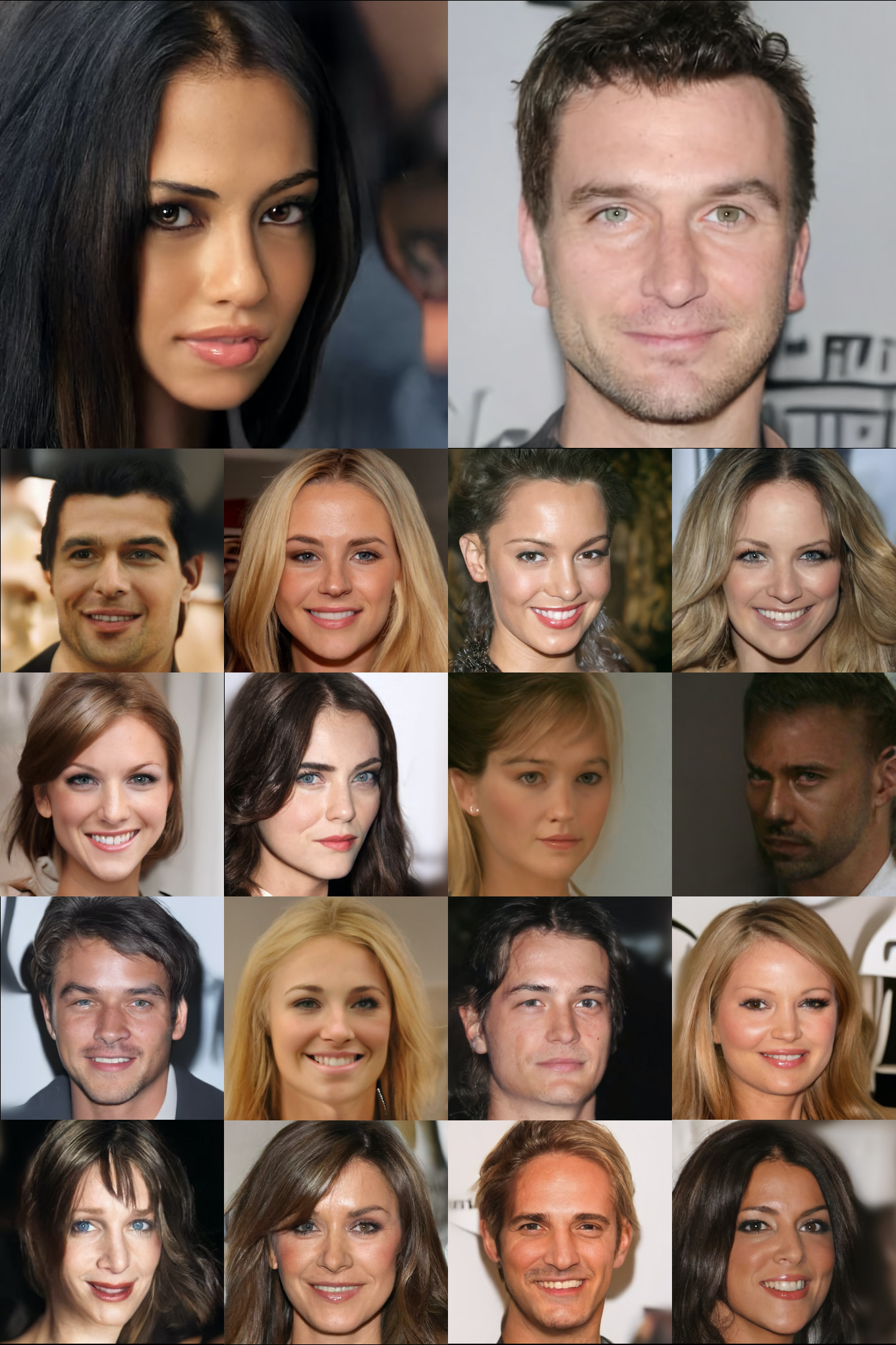
H.2 Results on CIFAR-10

All architecture components introduced above can improve the performance of score-based models trained with VE SDEs, as shown in Figure 22. The box plots demonstrate the importance of each component when other components can vary freely. On both CIFAR-10 and CelebA, the additional components that we explored always improve the performance on average for VE SDEs. For progressive growing, it is not clear which combination of configurations consistently performs the best, but the results are typically better than when no progressive growing architecture is used. Our best score-based model for VE SDEs 1) uses FIR upsampling/downsampling, 2) rescales skip connections, 3) employs BigGAN-type residual blocks, 4) uses 4 residual blocks per resolution instead of 2, and 5) uses "residual" for input and no progressive growing architecture for output. We name this model "NCSN++", following the naming convention of previous SMLD models ([1, 7]).

We followed a similar procedure to examine these architecture components for VP SDEs, except that we skipped experiments on CelebA due to limited computing resources. The NCSN++ architecture worked decently well for VP SDEs, ranked 4th place over all 144 possible configurations. The top configuration, however, has a slightly different structure, which uses no FIR upsampling/downsampling and no progressive growing architecture compared to NCSN++. We name this model "DDPM++", following the naming convention of [3].

The basic NCSN++ model with 4 residual blocks per resolution achieves an FID of 2.45 on CIFAR-10, whereas the basic DDPM++ model achieves an FID of 2.78. Here in order to match the convention used in [47, 1] and [3], we report the lowest FID value over the course of training, rather than the average FID value over checkpoints after 0.5M iterations (used for comparing different models of VE SDEs) or between 0.25M and 0.5M iterations (used for comparing VP SDE models) in our architecture exploration.

Switching from discrete training objectives to continuous ones in Equation 7 further improves the FID values for all SDEs. To condition the NCSN++ model on continuous time variables, we change positional embeddings, the layers in [3] for conditioning on discrete time steps, to random Fourier feature embeddings ([49]). The scale parameter of these random Fourier feature embeddings is fixed to 16. We also reduce the number of training iterations to 0.95M to suppress overfitting. These changes improve the FID on CIFAR-10 from 2.45 to 2.38 for NCSN++ trained with the VE SDE, resulting in a model called "NCSN++ cont.". In addition, we can further improve the FID from 2.38 to 2.20 by doubling the number of residual blocks per resolution for NCSN++ cont., resulting in the model denoted as "NCSN++ cont. (deep)". All quantitative results are summarized in Table 3, and we provide random samples from our best model in Figure 23.

Similarly, we can also condition the DDPM++ model on continuous time steps, resulting in a model "DDPM++ cont.". When trained with the VP SDE, it improves the FID of 2.78 from DDPM++ to 2.55. When trained with the sub-VP SDE, it achieves an FID of 2.61. To get better performance, we used the Euler-Maruyama solver as the predictor for continuously-trained models, instead of the ancestral sampling predictor or the reverse diffusion predictor. This is because the discretization strategy of the original DDPM method does not match the variance of the continuous process well when $t\to 0$, which significantly hurts FID scores. As shown in Table 2, the likelihood values are 3.21 and 3.05 bits/dim for VP and sub-VP SDEs respectively. Doubling the depth, and trainin with 0.95M iterations, we can improve both FID and bits/dim for both VP and sub-VP SDEs, leading to a model "DDPM++ cont. (deep)". Its FID score is 2.41, same for both VP and sub-VP SDEs. When trained with the sub-VP SDE, it can achieve a likelihood of 2.99 bits/dim. Here all likelihood values are reported for the last checkpoint during training.

H.3 High resolution images

Encouraged by the success of NCSN++ on CIFAR-10, we proceed to test it on $1024\times 1024$ CelebA-HQ ([47]), a task that was previously only achievable by some GAN models and VQ-VAE-2 ([50]). We used a batch size of 8, increased the EMA rate to 0.9999, and trained a model similar to NCSN++ with the continuous objective Equation (7) for around 2.4M iterations (please find the detailed architecture in our code release.) We use the PC sampler discretized at 2000 steps with the reverse diffusion predictor, one Langevin step per predictor update and a signal-to-noise ratio of 0.15. The scale parameter for the random Fourier feature embeddings is fixed to 16. We use the "input skip" progressive architecture for the input, and "output skip" progressive architecture for the output. We provide samples in Figure 24. Although these samples are not perfect (e.g, there are visible flaws on facial symmetry), we believe these results are encouraging and can demonstrate the scalability of our approach. Future work on more effective architectures are likely to significantly advance the performance of score-based generative models on this task.

I. Controllable generation

Consider a forward SDE with the following general form

$ \begin{align*} \mathrm{d} \mathbf{x} = \mathbf{f}(\mathbf{x}, t) \mathrm{d} t + \mathbf{G}(\mathbf{x}, t) \mathrm{d} \mathbf{w}, \end{align*} $

and suppose the initial state distribution is $p_0(\mathbf{x}(0) \mid \mathbf{y})$. The density at time $t$ is $p_t(\mathbf{x}(t) \mid \mathbf{y})$ when conditioned on $\mathbf{y}$. Therefore, using [12], the reverse-time SDE is given by

$ \begin{align} \displaystyle \mathrm{d} \mathbf{x} = {\mathbf{f}(\mathbf{x}, t) - \nabla \cdot [\mathbf{G}(\mathbf{x}, t) \mathbf{G}(\mathbf{x}, t)^{\mkern-1.5mu\mathsf{T}}] - \mathbf{G}(\mathbf{x}, t)\mathbf{G}(\mathbf{x}, t)^{\mkern-1.5mu\mathsf{T}} \nabla_\mathbf{x} \log p_t(\mathbf{x} \mid \mathbf{y})} \mathrm{d} t + \mathbf{G}(\mathbf{x}, t) \mathrm{d} \bar{\mathbf{w}} . \end{align}\tag{18} $

Since $p_t(\mathbf{x}(t) \mid \mathbf{y}) \propto p_t(\mathbf{x}(t)) p(\mathbf{y} \mid \mathbf{x}(t))$, the score $\nabla_\mathbf{x} \log p_t(\mathbf{x}(t) \mid \mathbf{y})$ can be computed easily by

$ \begin{align} \nabla_{\mathbf{x}} \log p_t(\mathbf{x}(t) \mid \mathbf{y}) = \nabla_{\mathbf{x}} \log p_t(\mathbf{x}(t)) + \nabla_{\mathbf{x}} \log p(\mathbf{y} \mid \mathbf{x}(t)). \end{align} $

This subsumes the conditional reverse-time SDE in Equation 14 as a special case. All sampling methods we have discussed so far can be applied to the conditional reverse-time SDE for sample generation.

I.1 Class-conditional sampling

When $\mathbf{y}$ represents class labels, we can train a time-dependent classifier $p_t(\mathbf{y} \mid \mathbf{x}(t))$ for class-conditional sampling. Since the forward SDE is tractable, we can easily create a pair of training data $(\mathbf{x}(t), \mathbf{y})$ by first sampling $(\mathbf{x}(0), \mathbf{y})$ from a dataset and then obtaining $\mathbf{x}(t) \sim p_{0t}(\mathbf{x}(t) \mid \mathbf{x}(0))$. Afterwards, we may employ a mixture of cross-entropy losses over different time steps, like Equation 7, to train the time-dependent classifier $p_t(\mathbf{y} \mid \mathbf{x}(t))$.

To test this idea, we trained a Wide ResNet ([51]) (Wide-ResNet-28-10) on CIFAR-10 with VE perturbations. The classifier is conditioned on $\log \sigma_i$ using random Fourier features ([49]), and the training objective is a simple sum of cross-entropy losses sampled at different scales. We provide a plot to show the accuracy of this classifier over noise scales in Figure 25. The score-based model is an unconditional NCSN++ (4 blocks/resolution) in Table 3, and we generate samples using the PC algorithm with 2000 discretization steps. The class-conditional samples are provided in Figure 4, and an extended set of conditional samples is given in Figure 25.

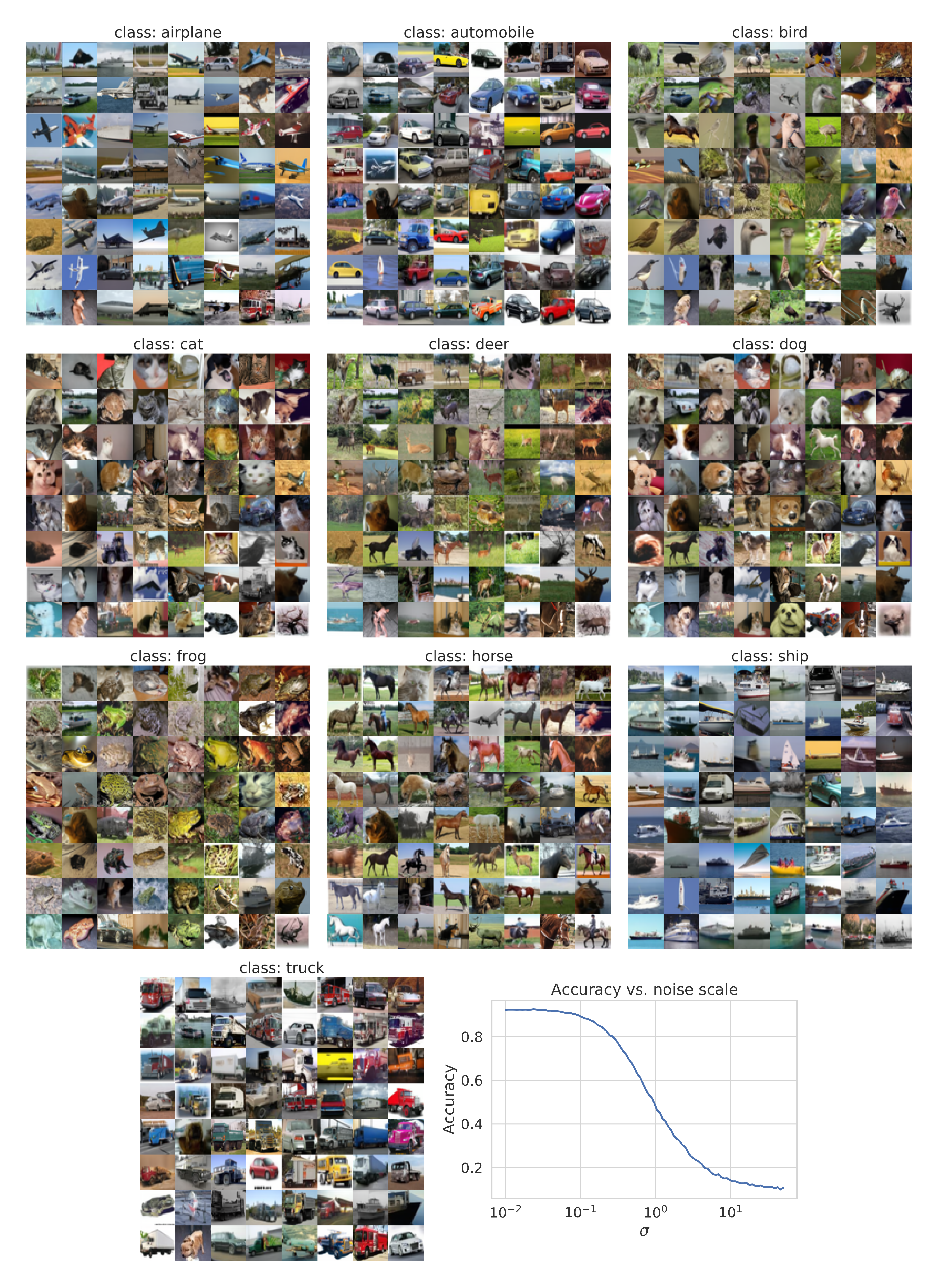
I.2 Imputation

Imputation is a special case of conditional sampling. Denote by $\Omega(\mathbf{x})$ and ${\bar{\Omega}}(\mathbf{x})$ the known and unknown dimensions of $\mathbf{x}$ respectively, and let $\mathbf{f}{{\bar{\Omega}}}(\cdot, t)$ and $\mathbf{G}{{\bar{\Omega}}}(\cdot, t)$ denote $\mathbf{f}(\cdot, t)$ and $\mathbf{G}(\cdot, t)$ restricted to the unknown dimensions. For VE/VP SDEs, the drift coefficient $\mathbf{f}(\cdot, t)$ is element-wise, and the diffusion coefficient $\mathbf{G}(\cdot, t)$ is diagonal. When $\mathbf{f}(\cdot, t)$ is element-wise, $\mathbf{f}{{\bar{\Omega}}}(\cdot, t)$ denotes the same element-wise function applied only to the unknown dimensions. When $\mathbf{G}(\cdot, t)$ is diagonal, $\mathbf{G}{{\bar{\Omega}}}(\cdot, t)$ denotes the sub-matrix restricted to unknown dimensions.

For imputation, our goal is to sample from $p({\bar{\Omega}}(\mathbf{x}(0)) \mid \Omega(\mathbf{x}(0)) = \mathbf{y})$. Define a new diffusion process $\mathbf{z}(t) = {\bar{\Omega}}(\mathbf{x}(t))$, and note that the SDE for $\mathbf{z}(t)$ can be written as

$ \begin{align*} \mathrm{d} \mathbf{z} = \mathbf{f}{\bar{\Omega}}(\mathbf{z}, t) \mathrm{d} t + \mathbf{G}{\bar{\Omega}}(\mathbf{z}, t) \mathrm{d} \mathbf{w}. \end{align*} $

The reverse-time SDE, conditioned on $\Omega(\mathbf{x}(0)) = \mathbf{y}$, is given by

$ \begin{split} \mathrm{d} \mathbf{z} = \big{\mathbf{f}{\bar{\Omega}}(\mathbf{z}, t) - \nabla \cdot [\mathbf{G}{{\bar{\Omega}}}(\mathbf{z}, t) \mathbf{G}{{\bar{\Omega}}}(\mathbf{z}, t)^{\mkern-1.5mu\mathsf{T}}] \- \mathbf{G}{\bar{\Omega}}(\mathbf{z}, t)\mathbf{G}{\bar{\Omega}}(\mathbf{z}, t)^{\mkern-1.5mu\mathsf{T}} \nabla\mathbf{z} \log p_t(\mathbf{z} \mid \Omega(\mathbf{z}(0)) = \mathbf{y})\big}\mathrm{d} t + \mathbf{G}_{\bar{\Omega}}(\mathbf{z}, t)\mathrm{d}\bar{\mathbf{w}}. \end{split} $

Although $p_t(\mathbf{z}(t) \mid \Omega(\mathbf{x}(0)) = \mathbf{y})$ is in general intractable, it can be approximated. Let $A$ denote the event $\Omega(\mathbf{x}(0)) = \mathbf{y} $. We have

$ \begin{align*} p_t(\mathbf{z}(t) \mid \Omega(\mathbf{x}(0)) = \mathbf{y}) = p_t(\mathbf{z}(t) \mid A) &= \int p_t(\mathbf{z}(t) \mid \Omega(\mathbf{x}(t)), A) p_t(\Omega(\mathbf{x}(t)) \mid A) \mathrm{d} \Omega(\mathbf{x}(t)) \ &= \mathbb{E}{p_t(\Omega(\mathbf{x}(t)) \mid A)}[p_t(\mathbf{z}(t) \mid \Omega(\mathbf{x}(t)), A)]\ &\approx \mathbb{E}{p_t(\Omega(\mathbf{x}(t)) \mid A)}[p_t(\mathbf{z}(t) \mid \Omega(\mathbf{x}(t)))]\ &\approx p_t(\mathbf{z}(t) \mid \hat{\Omega}(\mathbf{x}(t))), \end{align*} $

where $\hat{\Omega}(\mathbf{x}(t))$ is a random sample from $p_t(\Omega(\mathbf{x}(t)) \mid A)$, which is typically a tractable distribution. Therefore,

$ \begin{align*} \nabla_\mathbf{z} \log p_t(\mathbf{z}(t) \mid \Omega(\mathbf{x}(0))= \mathbf{y}) &\approx \nabla_\mathbf{z} \log p_t(\mathbf{z}(t) \mid \hat{\Omega}(\mathbf{x}(t))) \ &= \nabla_\mathbf{z} \log p_t([\mathbf{z}(t); \hat{\Omega}(\mathbf{x}(t))]), \end{align*} $

where $[\mathbf{z}(t); \hat{\Omega}(\mathbf{x}(t))]$ denotes a vector $\mathbf{u}(t)$ such that $\Omega(\mathbf{u}(t)) = \hat{\Omega}(\mathbf{x}(t))$ and $\bar{\Omega}(\mathbf{u}(t)) = \mathbf{z}(t)$, and the identity holds because $\nabla_\mathbf{z} \log p_t([\mathbf{z}(t); \hat{\Omega}(\mathbf{x}(t))]) = \nabla_\mathbf{z} \log p_t(\mathbf{z}(t) \mid \hat{\Omega}(\mathbf{x}(t))) + \nabla_\mathbf{z} \log p(\hat{\Omega}(\mathbf{x}(t))) = \nabla_\mathbf{z} \log p_t(\mathbf{z}(t) \mid \hat{\Omega}(\mathbf{x}(t)))$.

We provided an extended set of inpainting results in Figure 26 and Figure 27.

I.3 Colorization

Colorization is a special case of imputation, except that the known data dimensions are coupled. We can decouple these data dimensions by using an orthogonal linear transformation to map the gray-scale image to a separate channel in a different space, and then perform imputation to complete the other channels before transforming everything back to the original image space. The orthogonal matrix we used to decouple color channels is

$ \begin{align*} \begin{pmatrix} 0.577 & -0.816 & 0\ 0.577 & 0.408 & 0.707\ 0.577 & 0.408 & -0.707\ \end{pmatrix}. \end{align*} $

Because the transformations are all orthogonal matrices, the standard Wiener process $\mathbf{w}(t)$ will still be a standard Wiener process in the transformed space, allowing us to build an SDE and use the same imputation method in Appendix I.2. We provide an extended set of colorization results in Figure 28 and Figure 29.

I.4 Solving general inverse problems

Suppose we have two random variables $\mathbf{x}$ and $\mathbf{y}$, and we know the forward process of generating $\mathbf{y}$ from $\mathbf{x}$, given by $p(\mathbf{y} \mid \mathbf{x})$. The inverse problem is to obtain $\mathbf{x}$ from $\mathbf{y}$, that is, generating samples from $p(\mathbf{x} \mid \mathbf{y})$. In principle, we can estimate the prior distribution $p(\mathbf{x})$ and obtain $p(\mathbf{x} \mid \mathbf{y})$ using Bayes' rule: $p(\mathbf{x} \mid \mathbf{y}) = p(\mathbf{x}) p(\mathbf{y} \mid \mathbf{x}) / p(\mathbf{y})$. In practice, however, both estimating the prior and performing Bayesian inference are non-trivial.

Leveraging Equation 18, score-based generative models provide one way to solve the inverse problem. Suppose we have a diffusion process ${\mathbf{x}(t)}{t=0}^T$ generated by perturbing $\mathbf{x}$ with an SDE, and a time-dependent score-based model $\mathbf{s}{{\boldsymbol{\theta}}*}(\mathbf{x}(t), t)$ trained to approximate $\nabla_\mathbf{x} \log p_t(\mathbf{x}(t))$. Once we have an estimate of $\nabla_\mathbf{x} \log p_t(\mathbf{x}(t) \mid \mathbf{y})$, we can simulate the reverse-time SDE in Equation 18 to sample from $p_0(\mathbf{x}(0) \mid \mathbf{y}) = p(\mathbf{x} \mid \mathbf{y})$. To obtain this estimate, we first observe that

$ \begin{align*} \nabla_\mathbf{x} \log p_t(\mathbf{x}(t) \mid \mathbf{y}) = \nabla_\mathbf{x} \log \int p_t(\mathbf{x}(t) \mid \mathbf{y}(t), \mathbf{y}) p(\mathbf{y}(t) \mid \mathbf{y}) \mathrm{d} \mathbf{y}(t), \end{align*} $

where $\mathbf{y}(t)$ is defined via $\mathbf{x}(t)$ and the forward process $p(\mathbf{y}(t) \mid \mathbf{x}(t))$. Now assume two conditions:

• $p(\mathbf{y}(t) \mid \mathbf{y})$ is tractable. We can often derive this distribution from the interaction between the forward process and the SDE, like in the case of image imputation and colorization.
• $p_t(\mathbf{x}(t) \mid \mathbf{y}(t), \mathbf{y}) \approx p_t(\mathbf{x}(t) \mid \mathbf{y}(t))$. For small $t$, $\mathbf{y}(t)$ is almost the same as $\mathbf{y}$ so the approximation holds. For large $t$, $\mathbf{y}$ becomes further away from $\mathbf{x}(t)$ in the Markov chain, and thus have smaller impact on $\mathbf{x}(t)$. Moreover, the approximation error for large $t$ matter less for the final sample, since it is used early in the sampling process.

Given these two assumptions, we have

$ \begin{align} \nabla_\mathbf{x} \log p_t(\mathbf{x}(t) \mid \mathbf{y}) &\approx \nabla_\mathbf{x} \log \int p_t(\mathbf{x}(t) \mid \mathbf{y}(t)) p(\mathbf{y}(t) \mid \mathbf{y}) \mathrm{d} \mathbf{y} \notag\ &\approx \nabla_\mathbf{x} \log p_t(\mathbf{x}(t) \mid \hat{\mathbf{y}}(t)) \notag\ &= \nabla_\mathbf{x} \log p_t(\mathbf{x}(t)) + \nabla_\mathbf{x} \log p_t(\hat{\mathbf{y}}(t) \mid \mathbf{x}(t)) \notag\ &\approx \mathbf{s}{{\boldsymbol{\theta}}^*}(\mathbf{x}(t), t) + \nabla\mathbf{x} \log p_t(\hat{\mathbf{y}}(t) \mid \mathbf{x}(t)), \end{align}\tag{36} $

where $\hat{\mathbf{y}}(t)$ is a sample from $p(\mathbf{y}(t) \mid \mathbf{y})$. Now we can plug Equation 36 into Equation 18 and solve the resulting reverse-time SDE to generate samples from $p(\mathbf{x} \mid \mathbf{y})$.

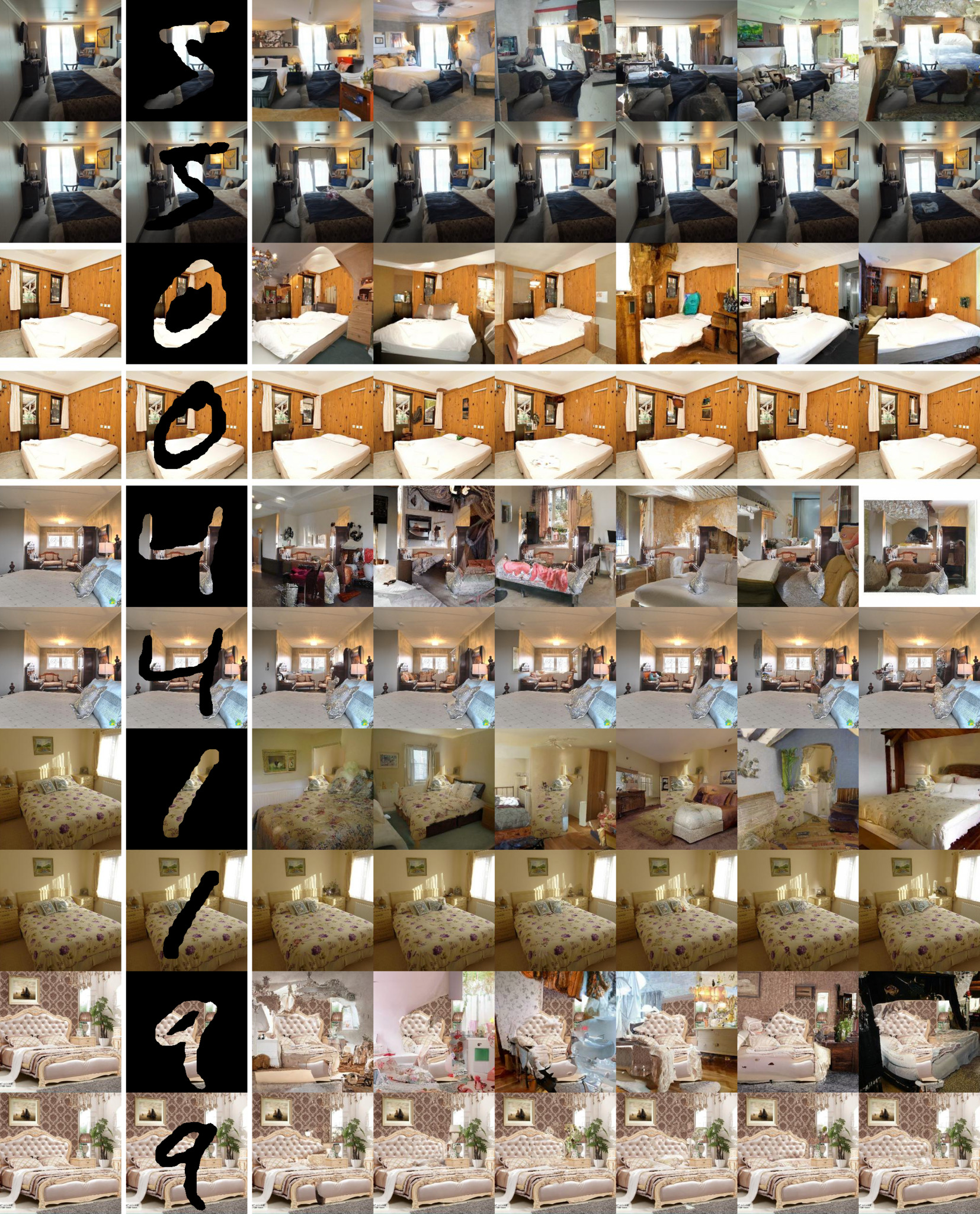
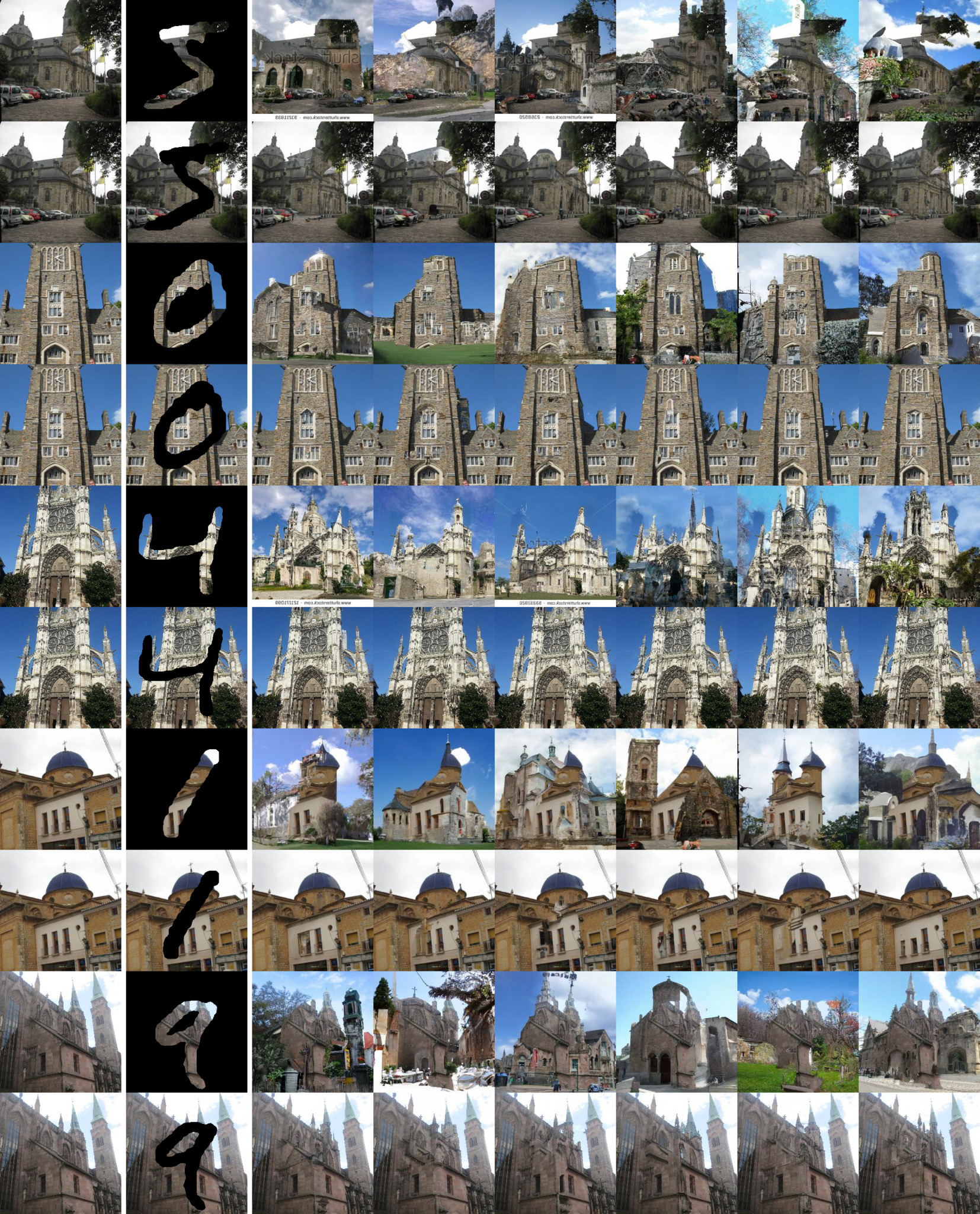
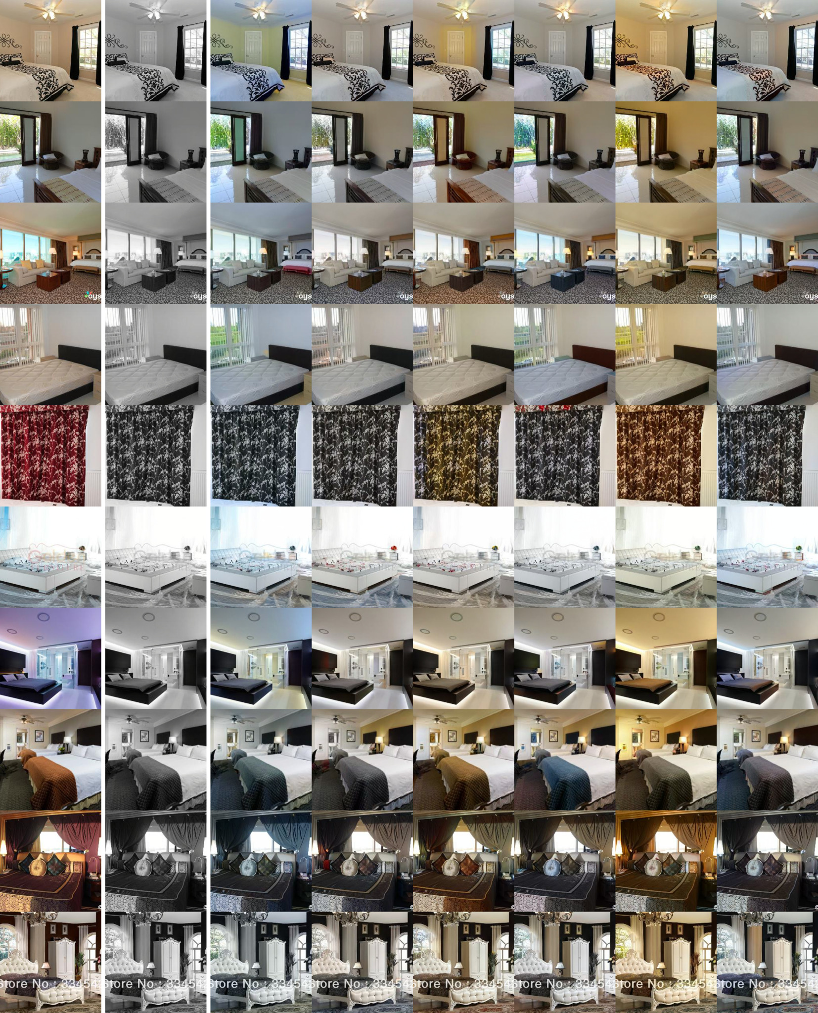
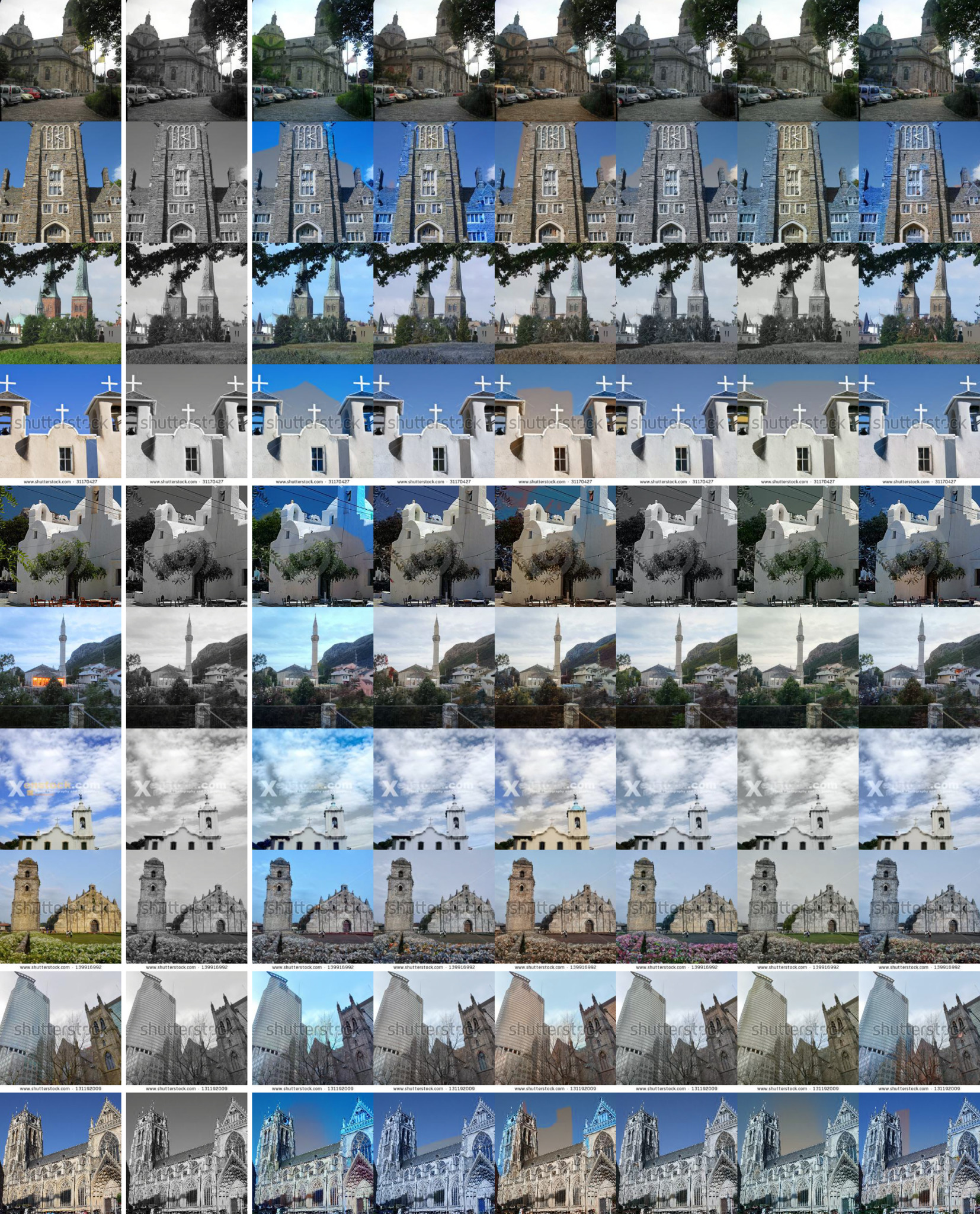
References

[1] Song, Yang and Ermon, Stefano (2019). Generative Modeling by Estimating Gradients of the Data Distribution. In Advances in Neural Information Processing Systems. pp. 11895–11907.

[2] Sohl-Dickstein et al. (2015). Deep Unsupervised Learning using Nonequilibrium Thermodynamics. In International Conference on Machine Learning. pp. 2256–2265.

[3] Ho et al. (2020). Denoising diffusion probabilistic models. Advances in Neural Information Processing Systems. 33.

[4] Bordes et al. (2017). Learning to generate samples from noise through infusion training. arXiv preprint arXiv:1703.06975.

[5] Goyal et al. (2017). Variational walkback: Learning a transition operator as a stochastic recurrent net. In Advances in Neural Information Processing Systems. pp. 4392–4402.

[6] Du, Yilun and Mordatch, Igor (2019). Implicit Generation and Modeling with Energy Based Models. In Advances in Neural Information Processing Systems. pp. 3608–3618.

[7] Song, Yang and Ermon, Stefano (2020). Improved techniques for training score-based generative models. Advances in Neural Information Processing Systems. 33.

[8] Chen et al. (2020). WaveGrad: Estimating Gradients for Waveform Generation. arXiv preprint arXiv:2009.00713.

[9] Kong et al. (2020). DiffWave: A Versatile Diffusion Model for Audio Synthesis. arXiv preprint arXiv:2009.09761.

[10] Niu et al. (2020). Permutation Invariant Graph Generation via Score-Based Generative Modeling. pp. 4474–4484.

[11] Cai et al. (2020). Learning Gradient Fields for Shape Generation. In Proceedings of the European Conference on Computer Vision (ECCV).

[12] Anderson, Brian D O (1982). Reverse-time diffusion equation models. Stochastic Process. Appl.. 12(3). pp. 313–326.

[13] Parisi, Giorgio (1981). Correlation functions and computer simulations. Nuclear Physics B. 180(3). pp. 378–384.

[14] Neal, Radford M and others (2011). MCMC using Hamiltonian dynamics. Handbook of markov chain monte carlo. 2(11). pp. 2.

[15] Vincent, Pascal (2011). A connection between score matching and denoising autoencoders. Neural computation. 23(7). pp. 1661–1674.

[16] Øksendal, Bernt (2003). Stochastic differential equations.

[17] Hyvärinen, Aapo (2005). Estimation of non-normalized statistical models by score matching. Journal of Machine Learning Research. 6(Apr). pp. 695–709.

[18] Yang Song et al. (2019). Sliced Score Matching: A Scalable Approach to Density and Score Estimation. In Proceedings of the Thirty-Fifth Conference on Uncertainty in Artificial Intelligence, UAI 2019, Tel Aviv, Israel, July 22-25, 2019. pp. 204.

[19] Pang et al. (2020). Efficient Learning of Generative Models via Finite-Difference Score Matching. arXiv preprint arXiv:2007.03317.

[20] Särkkä, Simo and Solin, Arno (2019). Applied stochastic differential equations. Cambridge University Press.

[21] Kloeden, Peter E and Platen, Eckhard (2013). Numerical solution of stochastic differential equations. Springer Science & Business Media.

[22] Grenander, Ulf and Miller, Michael I (1994). Representations of knowledge in complex systems. Journal of the Royal Statistical Society: Series B (Methodological). 56(4). pp. 549–581.

[23] Allgower, Eugene L and Georg, Kurt (2012). Numerical continuation methods: an introduction. Springer Science & Business Media.

[24] Chen et al. (2018). Neural ordinary differential equations. In Advances in neural information processing systems. pp. 6571–6583.

[25] Ho et al. (2019). Flow++: Improving Flow-Based Generative Models with Variational Dequantization and Architecture Design. In International Conference on Machine Learning. pp. 2722–2730.

[26] Dinh et al. (2016). Density estimation using real nvp. arXiv preprint arXiv:1605.08803.

[27] Behrmann et al. (2019). Invertible residual networks. In International Conference on Machine Learning. pp. 573–582.

[28] Kingma, Durk P and Dhariwal, Prafulla (2018). Glow: Generative flow with invertible 1x1 convolutions. In Advances in Neural Information Processing Systems. pp. 10215–10224.

[29] Song et al. (2019). MintNet: Building invertible neural networks with masked convolutions. In Advances in Neural Information Processing Systems. pp. 11002–11012.

[30] Chen et al. (2019). Residual flows for invertible generative modeling. In Advances in Neural Information Processing Systems. pp. 9916–9926.

[31] Grathwohl et al. (2018). FFJORD: Free-Form Continuous Dynamics for Scalable Reversible Generative Models. In International Conference on Learning Representations.

[32] Brock et al. (2018). Large Scale GAN Training for High Fidelity Natural Image Synthesis. In International Conference on Learning Representations.

[33] Karras et al. (2020). Training generative adversarial networks with limited data. Advances in Neural Information Processing Systems. 33.

[34] Roeder et al. (2020). On Linear Identifiability of Learned Representations. arXiv preprint arXiv:2007.00810.

[35] Dormand, John R and Prince, Peter J (1980). A family of embedded Runge-Kutta formulae. Journal of computational and applied mathematics. 6(1). pp. 19–26.

[36] Goodfellow et al. (2014). Generative adversarial nets. In Advances in neural information processing systems. pp. 2672–2680.

[37] Maoutsa et al. (2020). Interacting particle solutions of Fokker-Planck equations through gradient-log-density estimation. arXiv preprint arXiv:2006.00702.

[38] Skilling, John (1989). The eigenvalues of mega-dimensional matrices.

[39] Hutchinson, Michael F (1990). A stochastic estimator of the trace of the influence matrix for Laplacian smoothing splines. Communications in Statistics-Simulation and Computation. 19(2). pp. 433–450.

[40] Jolicoeur-Martineau et al. (2020). Adversarial score matching and improved sampling for image generation. arXiv preprint arXiv:2009.05475.

[41] Efron, Bradley (2011). Tweedie’s formula and selection bias. Journal of the American Statistical Association. 106(496). pp. 1602–1614.

[42] Yu et al. (2015). Lsun: Construction of a large-scale image dataset using deep learning with humans in the loop. arXiv preprint arXiv:1506.03365.

[43] Krizhevsky et al. (2009). Learning multiple layers of features from tiny images.

[44] Liu et al. (2015). Deep Learning Face Attributes in the Wild. In Proceedings of International Conference on Computer Vision (ICCV).

[45] Zhang, Richard (2019). Making Convolutional Networks Shift-Invariant Again. In ICML.

[46] Tero Karras et al. (2020). Analyzing and Improving the Image Quality of StyleGAN. In Proc. CVPR.

[47] Karras et al. (2018). Progressive Growing of GANs for Improved Quality, Stability, and Variation. In International Conference on Learning Representations.

[48] Karras et al. (2019). A style-based generator architecture for generative adversarial networks. In Proceedings of the IEEE Conference on Computer Vision and Pattern Recognition. pp. 4401–4410.

[49] Matthew Tancik et al. (2020). Fourier Features Let Networks Learn High Frequency Functions in Low Dimensional Domains. NeurIPS.

[50] Razavi et al. (2019). Generating diverse high-fidelity images with vq-vae-2. In Advances in Neural Information Processing Systems. pp. 14837–14847.

[51] Zagoruyko, Sergey and Komodakis, Nikos (2016). Wide residual networks. arXiv preprint arXiv:1605.07146.