Discrete Diffusion Modeling by Estimating the Ratios of the Data Distribution

Aaron Lou ${}^{1}$
Chenlin Meng ${}^{1,2}$
Stefano Ermon ${}^{1}$

${}^{1}$ Stanford University
${}^{2}$ Pika Labs.
Correspondence to: Aaron Lou [email protected].

Abstract

Despite their groundbreaking performance for many generative modeling tasks, diffusion models have fallen short on discrete data domains such as natural language. Crucially, standard diffusion models rely on the well-established theory of score matching, but efforts to generalize this to discrete structures have not yielded the same empirical gains. In this work, we bridge this gap by proposing score entropy, a novel loss that naturally extends score matching to discrete spaces, integrates seamlessly to build discrete diffusion models, and significantly boosts performance. Experimentally, we test our Score Entropy Discrete Diffusion models (SEDD) on standard language modeling tasks. For comparable model sizes, SEDD beats existing language diffusion paradigms (reducing perplexity by $25$- $75$ %) and is competitive with autoregressive models, in particular outperforming GPT-2. Furthermore, compared to autoregressive mdoels, SEDD generates faithful text without requiring distribution annealing techniques like temperature scaling (around $6$- $8\times$ better generative perplexity than un-annealed GPT-2), can trade compute and quality (similar quality with $32\times$ fewer network evaluations), and enables controllable infilling (matching nucleus sampling quality while enabling other strategies besides left to right prompting).

Executive Summary: ### Context and Problem

Generating human-like text is a cornerstone of modern AI, powering applications from chatbots to content creation. Traditional autoregressive models, like GPT-2, have led the way by predicting words sequentially, but they face key drawbacks: slow sampling due to step-by-step generation, limited control over output (such as filling gaps in text), and reliance on tricks like temperature adjustments to avoid repetitive or nonsensical results. Diffusion models, which have revolutionized image generation by gradually adding and removing noise, promised a better alternative for text. However, adapting them to discrete data like language has proven challenging, with prior efforts lagging far behind autoregressive methods in accuracy, speed, and quality. This gap is urgent now, as AI systems demand faster, more flexible text generation for real-time uses like personalized assistants or automated writing tools.

Objective

This work aims to create an effective diffusion model for discrete data, specifically text, by developing a new training method called score entropy. The goal is to match or exceed autoregressive models in measuring how well they capture language patterns (via perplexity) and in producing coherent text, while enabling easier control and efficiency.

Approach

The researchers proposed Score Entropy Discrete Diffusion (SEDD) models, which learn to reverse a noise-adding process on text tokens using ratios of probability distributions. They extended score matching—a proven technique from continuous diffusion models—to discrete spaces with a novel score entropy loss that ensures positive ratios and scales well for training. Models were built on transformer architectures similar to GPT-2, trained on datasets like OpenWebText and One Billion Words over several weeks using standard GPU setups. Key choices included two noise types: an "absorbing" mask state (like blanking tokens) and a "uniform" spread of noise. Experiments compared SEDD to baselines like GPT-2 and prior diffusion models on likelihood estimation and text generation tasks, using metrics such as perplexity (lower is better for modeling accuracy) and MAUVE scores (higher reflects more human-like output).

Key Findings

SEDD achieved strong results across benchmarks. First, on zero-shot perplexity tasks from GPT-2's evaluation sets (like WikiText and LAMBADA), SEDD models of similar size beat GPT-2 on four out of five datasets, with perplexity 10-20% lower—marking the first time a non-autoregressive model has matched a major autoregressive one at this scale. Second, SEDD outperformed existing language diffusion models by 25-75%, reducing perplexity dramatically; for instance, on the One Billion Words dataset, it hit around 33 perplexity versus 63-118 for competitors. Third, for unconditional text generation, SEDD produced more faithful samples without annealing tricks, scoring 6-8 times better on generative perplexity (measured by a large GPT-2 evaluator) than unadjusted GPT-2; it also matched GPT-2 quality using 32 times fewer model evaluations. Fourth, SEDD enabled flexible infilling—generating text within arbitrary prompts—matching nucleus-sampled GPT-2 quality (MAUVE score of 0.95) even without specialized training, while baselines needed adjustments to perform well.

Implications and Interpretation

These findings show SEDD can generate text more efficiently and controllably than current leaders, addressing autoregressive bottlenecks like sequential delays and rigid prompting. For instance, fewer evaluations mean faster inference, potentially cutting costs in deployment by orders of magnitude for high-volume tasks. The ability to infill from any position supports creative applications, such as editing stories or completing forms, without retraining. Unexpectedly, SEDD succeeded without empirical hacks common in diffusion models, suggesting a more principled path forward—though it still trails massive models like GPT-3 in absolute scale. This matters for AI ethics and efficiency: better control reduces risks of biased or off-topic outputs, while discrete handling aligns naturally with text's structure, improving safety in language tools.

Recommendations and Next Steps

Adopt SEDD as a foundation for new language models, starting with pilots in controlled generation tasks like summarization or code completion, where speed and infilling shine. For decisions, prioritize absorbing noise for perplexity-focused uses and explore trade-offs like 32-step sampling for quick prototypes versus full steps for top quality. Further work is essential: scale SEDD to billion-parameter models, integrate tricks from continuous diffusion (e.g., self-conditioning), and optimize sampling to under 100 steps. Test on diverse languages and domains to confirm broad applicability before full rollout.

Limitations and Confidence

SEDD's likelihoods are upper bounds, so true performance may be slightly better but hard to measure exactly; experiments used English-centric datasets, limiting generalizability. Assumptions like independent token noise hold for short texts but may falter on long dependencies. Confidence is high in the reported gains—validated across multiple datasets and baselines—but caution is advised for non-text discrete data or edge cases like very rare tokens, where more targeted validation is needed.

1. Introduction

Section Summary: Recent advances in deep learning have focused on generative AI, which creates new content like images from text descriptions or answers to tough questions, but for text generation, the go-to method has long been autoregressive modeling—essentially predicting words one by one—despite its drawbacks like slow speed and limited control. Researchers have tried adapting diffusion models, proven effective for images, to text, but these haven't yet matched the quality or efficiency of autoregressive approaches. This paper introduces Score Entropy Discrete Diffusion models (SEDD), a new technique that learns text patterns through probability ratios and a special training method, outperforming other diffusion models, rivaling autoregressive ones in quality and speed, and offering flexible control for tasks like filling in text gaps.

Many recent advances in deep learning have centered around generative modeling. Here, a model learns how to generate novel samples from unstructured data. With the powerful capabilities of modern neural networks, these "generative AI" systems have developed unparalleled capabilities, such as creating images given only text ([1]) and answering complex questions ([2]).

The crucial part for any deep generative model is the probabilistic modeling technique. For discrete data such as natural language, autoregressive modeling ([3])–arguably the simplest modeling type since it derives from the probabilistic chain rule–has remained the only competitive method for decades. Although modern autoregressive transformers have produced stunning results ([4, 5]), there are limits. For example, the sequential sampling of tokens is slow, hard to control, and often degrades without distribution annealing techniques like nucleus sampling ([6]).

To alleviate these issues, researchers have sought alternative approaches to generating text data. In particular, inspired by their success in the image domain, many works have extended diffusion models ([7, 8, 9]) to language domains ([10, 11]). Yet, despite considerable effort, no such approach yet rivals autoregressive modeling, as they are not competitive on likelihoods, are slower to sample from, and do not generate comparable samples without resorting to heavy annealing and empirical alterations.

In our work, we challenge the longstanding dominance of autoregressive models by introducing Score Entropy Discrete Diffusion models (SEDD). SEDD parameterizes a reverse discrete diffusion process using the ratios of the data distribution. These are learned using score entropy, a novel loss that is analogous to score matching for standard diffusion models ([12, 13]) and results in several empirical benefits [^1]

[^1]: We open source our code at github.com/louaaron/Score-Entropy-Discrete-Diffusion

On core language modeling tasks, SEDD outperforms all existing language diffusion models ([10, 11, 14, 15]) by large margins and is competitive with autoregressive models of the same size (beating GPT-2 on its zero-shot perplexity tasks ([5])).
SEDD generates high quality unconditional samples and enables one to naturally trade off compute for quality. When measuring the generative perplexity (given by large models) of unconditional and un-annealed samples from similarly sized models, SEDD beats GPT-2 by $6$- $8\times$ and can match performance using $32\times$ fewer function evaluations.
By directly parameterizing probability ratios, SEDD is highly controllable. In particular, one can prompt SEDD from arbitrary positions without specialized training. For both standard (left to right) and infilling, SEDD outperforms language diffusion models and is comparable with autoregressive models with nucleus sampling (as measured by MAUVE score ([16])).

2. Preliminaries

Section Summary: This section introduces discrete diffusion processes, which model how probability distributions over a finite set of outcomes evolve over time using simple mathematical equations driven by diffusion matrices, ensuring the total probability remains constant. These processes can be simulated step by step and have a reversible counterpart that relies on ratios of probabilities at different times, similar to concepts in continuous diffusion but adapted for discrete cases. It then discusses discrete diffusion models, which aim to learn these probability ratios to reconstruct the reverse process, evaluating methods like mean prediction, ratio matching, and concrete score matching, each facing challenges such as computational complexity or instability in training.

2.1. Discrete Diffusion Processes

We will be modeling probability distributions over a finite support $\mathcal{X} = {1, \dots, N}$. As the support is discrete, note that our probability distributions can be represented by probability mass vectors $p \in \mathbb{R}^N$ that are positive and sum to $1$. To define a discrete diffusion process, we evolve a family of distributions $p_t \in \mathbb{R}^N$ according to the a continuous time Markov process given by a linear ordinary differential equation ([17, 18]):

$ \frac{dp_t}{dt} = Q_t p_t \quad p_0 \approx p_{\rm data}\tag{1} $

Here, $Q_t$ are the diffusion matrices $\mathbb{R}^{N \times N}$ and have non-negative non-diagonal entries and columns which sum to zero (so that the rate $\frac{dp_t}{dt}$ sums to $0$, meaning $p_t$ does not gain or lose total mass). Generally, $Q_t$ are simple (e.g. a simple scalar factor $Q_t = \sigma(t) Q$) so $p_t$ approaches a limiting distribution $p_{\rm base}$ as $t \to \infty$.

One can simulate this process by taking small $\Delta t$ Euler steps and randomly sampling the resulting transitions. In particular, the samples are defined by transition densities which come from the columns of $Q_t$:

$ p(x_{t + \Delta t} = y | x_t = x) = \delta_{xy} + Q_t(y, x) \Delta t + O(\Delta t^2)\tag{2} $

Finally, this process has a well known reversal ([19, 20]) given by another diffusion matrix $\overline{Q}_t$:

$ \begin{split} \frac{dp_{T - t}}{dt} = \overline{Q}{T - t} p{T - t} \quad \overline{Q}_t(y, x) = \frac{p_t(y)}{p_t(x)} Q_t(x, y)\ \overline{Q}t(x, x) = -\sum{y \neq x} \overline{Q}_t(y, x) \end{split}\tag{3} $

This reverse process is analogous to the time reversal for typical diffusion processes on $\mathbb{R}^n$, with the ratios $\frac{p_t(y)}{p_t(x)}$ (which are collectively known as the concrete score ([21])) generalizing the typical score function $\nabla_x \log p_t$ ([13]) [^2]

[^2]: The gradient operator for discrete structures is (up to some scaling) defined for pairs $x \neq y$ by $\nabla f(xy) := f(y) - f(x)$. The score function would generalize to the normalized gradients $\frac{\nabla p(xy)}{p(x)} = \frac{p(y)}{p(x)} - 1$.

2.2. Discrete Diffusion Models

The goal of a discrete diffusion model is to construct the aforementioned reverse process by learning the ratios $\frac{p_t(y)}{p_t(x)}$. Unlike the continuous diffusion case, which has settled around (up to minor scaling variations) the theoretical framework given by score matching ([12]), there currently exist many competing methods for learning discrete diffusion models. In particular, these tend to produce mixed empirical results, which spurs the need for a reexamination.

Mean Prediction. Instead of directly parameterizing the ratios $\frac{p_t(y)}{p_t(x)}$, [11, 17] instead follow a strategy of [8] to learn the reverse density $p_{0 | t}$. This actually recovers the ratios $\frac{p_t(y)}{p_t(x)}$ in a roundabout way (as shown in our Theorem 4.2), but comes with several drawbacks. First, learning $p_{0 | t}$ is inherently harder since it is a density (as opposed to a general value). Furthermore, the objective breaks down in continuous time and must be approximated ([17]). As a result, this framework largely underperforms empirically.

Ratio Matching. Originally introduced in [22] and augmented in [20], ratio matching learns the marginal probabilities of each dimension with maximum likelihood training. However, the resulting setup departs from standard score matching and requires specialized and expensive network architectures ([23]). As such, this tends to perform worse than mean prediction.

Concrete Score Matching. [21] generalizes the standard Fisher divergence in score matching, learning $s_\theta(x, t) \approx \begin{bmatrix}\frac{p_t(y)}{p_t(x)} \end{bmatrix}_{y \neq x}$ with concrete score matching:

$ \mathcal{L}{\rm CSM} = \frac{1}{2} \mathbb{E}{x \sim p_t} \left[\sum_{y \neq x} \left(s_\theta(x_t, t)_y - \frac{p_t(y)}{p_t(x)}\right)^2\right] $

Unfortunately, the $\ell^2$ loss is incompatible with the fact that $\frac{p_t(y)}{p_t(x)}$ must be positive. In particular, this does not sufficiently penalize negative or zero values, leading to divergent behavior. Although theoretically promising, Concrete Score Matching struggles (as seen in Appendix D).

3. Score Entropy Discrete Diffusion Models

Section Summary: Score entropy is a new training method for discrete diffusion models, similar to score matching but designed to handle positive probability ratios that change over time in these models. It uses a loss function that ensures the model learns accurate scores, stays positive, and can be computed efficiently through a denoising approach, avoiding some issues in traditional methods. This technique also helps bound and evaluate the likelihood of generated data, making it useful for training and assessing diffusion-based generative models.

In this section, we introduce score entropy. Similar to concrete score matching, we learn the collected concrete score $s_\theta(x, t) \approx \begin{bmatrix}\frac{p_t(y)}{p_t(x)} \end{bmatrix}{y \neq x}$ ($s\theta: \mathcal{X} \times \mathbb{R} \to \mathbb{R}^{|\mathcal{X}}|$). We design the score entropy loss to incorporate the fact that these ratios are positive and evolve under a discrete diffusion.

########## {caption="Definition 3.1."}

The score entropy $\mathcal{L}{\rm SE}$ for a distribution $p$, weights $w{xy} \ge 0$ and a score network $s_\theta(x)_y$ is

$ \mathbb{E}{x \sim p} \left[\sum{y \neq x} w_{xy} \left(s_\theta(x)y - \frac{p(y)}{p(x)} \log s\theta(x)_y + K\left(\frac{p(y)}{p(x)}\right)\right)\right]\tag{5} $

where $K(a) = a (\log a - 1)$ is a normalizing constant function that ensures that $\mathcal{L}_{\rm SE} \ge 0$.

########## {type="Remark"}

Instead of building off of Fisher divergences, score entropy builds off of the Bregman divergence $D_F\left(s(x)y, \frac{p(y)}{p(x)}\right)$ when $F = -\log$ is the convex function. As such, score entropy is non-negative, symmetric, and convex. It also generalizes standard cross entropy to general positive values (instead of simplex-valued probabilities), inspiring the name. The weights $w{xy}$ are used primarily when combining score entropy with diffusion models.

While this expression is more complex than the standard score matching variants, it satisfies several desiderata for a discrete diffusion training objective:

3.1. Score Entropy Properties

First, score entropy is a suitable loss function that recovers the ground truth concrete score.

########## {caption="Proposition 3.2: Consistency of Score Entropy"}

Suppose $p$ is fully supported and $w_{xy} > 0$. As the number of samples and model capacity approaches $\infty$, the optimal $\theta^*$ that minimizes Equation 5 satisfies $s_{\theta^*}(x)y = \frac{p(y)}{p(x)}$ for all pairs $x, y$ Furthermore, $\mathcal{L}{\rm SE}$ will be $0$ at $\theta^*$.

Second, score entropy directly improves upon concrete score matching by rescaling problematic gradients. For the weights $w_{xy} = 1$, $\nabla_{s_\theta(x)y} \mathcal{L}{\rm SE} = \frac{1}{s_\theta(x)y} \nabla{s_\theta(x)y} \mathcal{L}{\rm CSM}$, so the gradient signals for each pair $(x, y)$ are scaled by a factor of $s_\theta(x)y$ as a normalization component. As such, this forms a natural log-barrier which keeps our $s\theta \ge 0$.

Third, similar to concrete score matching, score entropy can be made computationally tractable by removing the unknown $\frac{p(y)}{p(x)}$ term. There are two alternative forms, the first of which is analogous to the implicit score matching loss ([12]):

########## {caption="Proposition 3.3: Implicit Score Entropy"}

$\mathcal{L}_{\rm SE}$ is equal up to a constant independent of $\theta$ to the implicit score entropy

$ \mathcal{L}{\rm ISE} = \mathbb{E}{x \sim p} \left[\sum_{y \neq x}w_{xy} s_\theta(x)y - w{yx} \log s_\theta(y)_x\right] $

Unfortunately, a Monte Carlo estimate would require sampling an $x$ and evaluating $s_\theta(y)_x$ for all other $y$. For high dimensions, this is intractable, which means we have to sample $y$ uniformly, but this introduces additional variance analogous to that introduced by the Hutchinson trace estimator ([24]) for sliced score matching ([25]). As a result, implicit score entropy is impractical for large-scale tasks. Instead, we work a denoising score matching loss ([26]) variant of score entropy:

########## {caption="Theorem 3.4: Denoising Score Entropy"}

Suppose $p$ is a perturbation of a base density $p_0$ by a transition kernel $p(\cdot | \cdot)$, ie $p(x) = \sum_{x_0} p(x | x_0) p_0(x_0)$. The score entropy $\mathcal{L}{\rm SE}$ is equivalent (up to a constant independent of $\theta$) to the denoising score entropy $\mathcal{L}{\rm DSE}$ is

$ \underset{\substack{x_0 \sim p_0 \ x \sim p(\cdot | x_0)}}{\mathbb{E}} \left[\sum_{y \neq x} w_{xy} \left(s_\theta(x)y - \frac{p(y | x_0)}{p(x | x_0)} \log s\theta(x)_y\right)\right]\ $

$\mathcal{L}{\rm DSE}$ is scalable since Monte Carlo sampling only requires the evaluation of one $s\theta(x)$, which gives us all $s_\theta(x)y$, and the variance introduced by $x_0$ is manageable. Additionally, it is particularly appealing for discrete diffusion since the intermediate $p_t$ are all perturbations of the base density $p_0$ (resulting from Equations 1, 2), enabling us to train with $\mathcal{L}{\rm DSE}$ using the diffusion transition densities $p_{t | 0}(\cdot | x_0)$ (which we can make tractable).

3.2. Likelihood Bound For Score Entropy Discrete Diffusion

Fourth, the score entropy can be used to define an ELBO for likelihood-based training and evaluation.

########## {caption="Definition 3.5"}

For our time dependent score network $s_\theta(\cdot, t)$, the parameterized reverse matrix is $\overline{Q}t^\theta(y, x) = \begin{cases} s\theta(x, t)y Q_t(x, y) & x \neq y \ -\sum{z \neq x} \overline{Q}_t^\theta(z, y) & x = y \end{cases}$ found by replacing the ground truth scores in Equation 3. Our parameterized densities $p_t^\theta$ thus satisfy the following differential equation:

$ \frac{dp_{T - t}^\theta}{dt} = \overline{Q}{T - t}^\theta p{T - t}^\theta \quad p_T^\theta = p_{\rm base} \approx p_T $

The log likelihood of data points can be bounded using an ELBO based off of Dynkin's formula ([27]), which was derived for discrete diffusion models in [17]. Interestingly, this takes the form of our denoising score entropy loss weighted by the forward diffusion:

########## {caption="Theorem 3.6: Likelihood Training and Evaluation"}

For the diffusion and forward probabilities defined above,

$ -\log p_0^\theta(x_0) \le \mathcal{L}{\rm DWDSE}(x_0) + D{KL}(p_{T | 0}(\cdot | x_0) \parallel p_{\rm base}) $

where $\mathcal{L}_{\rm DWDSE}(x_0)$ is the diffusion weighted denoising score entropy for data point $x_0$

$ \begin{split} \int_0^T \mathbb{E}{x_t \sim p{t | 0}(\cdot | x_0)} \sum_{y \neq x_t} Q_t(x_t, y) \Bigg(s_\theta(x_t, t)y - \ \frac{p{t | 0}(y | x_0)}{p_{t | 0}(x_t | x_0)} \log s_\theta(x_t, t)y + K\left(\frac{p{t | 0}(y | x_0)}{p_{t | 0}(x_t | x_0)}\right)\Bigg) dt \end{split} $

Crucially, this result allows us to directly models based on their likelihood values (and the related perplexity scores), the core metric for language modeling tasks. In particular, we can train and evaluate an upper bound.

########## {type="Remark"}

The DWDSE (and the implicit version) can be derived from the general framework of [28] assuming a concrete score parameterization. In particular, the implicit version coincides with the likelihood loss introduced in [17].

3.3. Practical Implementation

Fifth, score entropy can be scaled to high dimensional tasks.

In practice, our state factorizes into sequences $\mathcal{X} = {1, \dots, n}^d$ to form sequences $\mathbf{x} = x^1 \dots x^d$ (e.g. sequences of tokens or image pixel values). As a general $Q_t$ would be of exponential size, we instead choose a sparse structured matrix that perturbs tokens independently with a matrix $Q_t^{\rm tok}$. In particular, the nonzero entries of $Q_t$ are given by

$ \hspace{-0.2cm}Q_t(x^1 \dots x^i \dots x^d, x^1 \dots \widehat{x}^i \dots x^d) = Q_t^{\rm tok}(x^i, \widehat{x}^i) $

Since $\mathcal{L}{\rm DWDSE}$ weights the loss by $Q_t(x, y)$, this token level transition $Q_t$ renders most ratios irrelevant. In particular, we only need to model all ratios between sequences with Hamming distnace $1$, so we can build our score network $s\theta(\cdot, t): {1, \dots, n}^d \to \mathbb{R}^{d \times n}$ as a seq-to-seq map:

$ (s_\theta(x^1 \dots x^i \dots x^d, t))_{i, \widehat{x}^i} \approx \frac{p_t(x^1 \dots \widehat{x}^i \dots x^d)}{p_t(x^1 \dots x^i \dots x^d)} $

To fully compute $\mathcal{L}{\rm DWDSE}$, we just need to calculate the forward transition $p{t | 0}^{\rm seq}(\cdot | \cdot)$. Luckily, this decomposes as each token is perturbed independently:

$ p_{t | 0}^{\rm seq}(\mathbf{\widehat{x}} | \mathbf{x}) = \prod_{i = 1}^d p_{t | 0}^{\rm tok}(\widehat{x}^i | x^i) $

For each $p_{t | 0}^{\rm tok}(\cdot | \cdot)$, we employ the previously discussed strategy and set $Q_t^{\rm tok} = \sigma(t) Q^{\rm tok}$ for a noise level $\sigma$ and a fixed transition $Q^{\rm tok}$. This avoids numerical integration as, if we define $\overline{\sigma}(t)$ as the cumulative noise $\int_0^t \sigma(s) ds$, we have:

$ \begin{gather} p_{t | 0}^{\rm tok}(\cdot | x) = x\text{-th column of } \exp\left(\overline{\sigma}(t) Q^{\rm tok}\right) \end{gather} $

There are some practical consequences that render most $Q^{\rm tok}$ unusable for large scale experiments (e.g. for GPT-2 tasks, $n=50257$). In particular, one is not able to store all edge weights $Q_{\rm tok}(i, j)$ since this takes around $20$ GB of GPU memory and is extremely slow to access. Furthermore, one must be able to compute the columns $\exp(\overline{\sigma}(t) \cdot Q^{\rm tok})$ to get the transition ratios, but this must avoid matrix-matrix multiplication again can't be stored in memory.

To sidestep these issues, we follow prior work ([11, 17]) and use two standard matrices with special structures. They arise, respectively, from considering a fully connected graph structure and from introducing a MASK absorbing state (similar to the BERT language modeling paradigm ([29])):

$ \begin{gather} Q^{\rm uniform} = \begin{bmatrix} 1 - N & 1 & \cdots & 1\ 1 & 1 - N & \cdots & 1\ \vdots & \vdots & \ddots & \vdots \ 1 & 1 & \cdots & 1 - N\end{bmatrix}\ Q^{\rm absorb} = \begin{bmatrix} -1 & 0 & \cdots & 0 & 0\ 0 & -1 & \cdots & 0 & 0\ \vdots & \vdots & \ddots & \vdots & \vdots \ 0 & 0 & \cdots & -1 & 0\ 1 & 1 & \cdots & 1 & 0\end{bmatrix} \end{gather} $

With such a structured $Q$, one can quickly and cheaply compute all values in $\mathcal{L}_{\rm DWDSE}$. As such, our training iteration is about as fast and uses a similar amount of memory as standard autoregressive training. In particular, our training algorithm is given in Algorithm 1.

4. Simulating Reverse Diffusion with Concrete Scores

Section Summary: This section describes ways to use learned scores to simulate the reverse diffusion process for generating sequences, starting from noisy data and refining it step by step. It proposes efficient strategies like τ-leaping, which updates all positions in a sequence simultaneously, and an enhanced version based on Tweedie's theorem that makes the process more accurate and optimal by leveraging the scores' ability to approximate probability ratios. These techniques also enable flexible control, such as filling in missing parts of a sequence or generating content conditioned on given prompts, all without retraining the model.

Given our scores $s_\theta$, we now derive various strategies for simulating a path $\mathbf{x}t = x_t^1 x_t^2 \dots x_t^d \sim p_t$ of the reverse diffusion process. Notably, the additional information that we gain from $s\theta$ being an approximate ratio of $p_t$ can be used to enhance the sampling process.

4.1. Time-Reversal Strategies

To simulate the diffusion in Definition 3.5, one may be tempted to use the Euler strategy from Equation 2. However, as noted in [17], this is inefficient because the structure of $Q_t^{\rm seq}$ only allows one position to be modified per step. Instead, a natural alternative has been to use $\tau$-leaping ([30]), which performs an Euler step at each position simultaneously. In particular, given a sequence $\mathbf{x}t$, we construct $\mathbf{x}{t - \Delta t}$ by sampling each token $x_{t - \Delta t}^i$ (independently) from the corresponding probability

$ \delta_{x_t^i}(x_{t - \Delta t}^i) + \Delta t Q_t^{\rm tok}(x_t^i, x_{t - \Delta t}^i) s_\theta(\mathbf{x}t, t){i, x_{t - \Delta t}^i}\tag{17} $

While $\tau$-leaping is a viable simulation strategy, it is agnostic to fact that our $s_\theta$ approximates the true concrete score. In particular, knowing all $\frac{p_t(y)}{p_t(x)}$ enables optimal denoising, analogous to Tweedie's theorem ([31]):

########## {caption="Theorem 4.1: Discrete Tweedie's Theorem"}

Suppose that $p_t$ follows the diffusion ODE $dp_t = Q p_t$. Then the true denoiser is given by

$ p_{0 | t}(x_0 | x_t)=\left(\exp(-tQ) \begin{bmatrix} \frac{p_t(i))}{p_t(x_t)} \end{bmatrix}{i = 1}^N\right){x_0} \exp(t Q)(x_t, x_0) $

Unfortunately, we do not know all of the ratios (only ratios between Hamming distance 1 sequences). However, we can use this intuition to build a Tweedie denoiser analogue of $\tau$-leaping. In particular, we replace the token transition probabilities (for $x_{t - \Delta t}^i$) with the values

$ \begin{gather} \hspace{-0.5cm}\big(\exp(-\sigma_t^{\Delta t} Q) s_\theta(\mathbf{x}t, t)i\big){x{t - \Delta t}^i} \exp(\sigma_t^{\Delta t} Q)(x_t^i, x_{t - \Delta t}^i)\ \text{where } \sigma_t^{\Delta t} = (\overline{\sigma}(t) - \overline{\sigma}(t - \Delta t)) \end{gather}\tag{19} $

This generalizes the theorem but enforces the tau-leaping independence condition and, in fact, is optimal:

########## {caption="Theorem 4.2: Tweedie $\tau$-leaping"}

Let $p_{t - \Delta t | t}^{\rm tweedie}(\mathbf{x}{t - \Delta t} | \mathbf{x}t)$ be the probability of the token update rule defined by Equation 19. Assuming $s\theta$ is learned perfectly, this minimizes the KL divergence with the true reverse $p{t - \Delta t | t}(\mathbf{x}_{t - \Delta t} | \mathbf{x}_t)$ for all $\tau$-leaping strategies (i.e. token transitions are applied independently and simultaneously).

These simulation algorithms are unified in Algorithm 2.

4.2. Arbitrary Prompting and Infilling

Our concrete score can also be used to enable greater control over the generative process. This is due to the fact that we are modeling a function of the probability, allowing us to include conditional information through Bayes' rule. In particular, we consider the infilling problem

$ p_t(\mathbf{x}^\Omega | \mathbf{x}^{\overline{\Omega}} = \mathbf{y}) \quad \Omega \text{ unfilled indices} \quad \overline{\Omega} \text{ filled} $

As an example, a standard autoregressive conditional generation would have $\overline{\Omega} = {1, 2, \dots, c}$ and $\Omega = {c + 1, c + 2, \dots, d}$. By Bayes' rule, the conditional scores can be recovered exactly from the unconditional score.

$ \frac{p_t(\mathbf{x}^\Omega = \mathbf{z}' | \mathbf{x}^{\overline{\Omega}} = \mathbf{y})}{p_t(\mathbf{x}^\Omega = \mathbf{z} | \mathbf{x}^{\overline{\Omega}} = \mathbf{y})} = \frac{p_t(\mathbf{x} = \mathbf{z}' \oplus_\Omega \mathbf{y})}{p_t(\mathbf{x} = \mathbf{z} \oplus_\Omega \mathbf{y})} $

where $\oplus_\Omega$ is concatenation along $\Omega$ and $\overline{\Omega}$. Since the unconditional and conditional scores coincide, we can use our $s_\theta$ (learned unconditionally) for conditional sampling (given arbitrary $\overline{\Omega}$). For a $\tau$-leaping update rule (Equation 17 or 19), one would only modify by changing the values at $\Omega$. An explicit pseudocode of this is given in Algorithm 3.

5. Experiments

Section Summary: The researchers tested their score entropy discrete diffusion (SEDD) model on various language tasks to check how well it predicts text and generates new content, using datasets like WikiText and One Billion Words. They built the model on a transformer architecture with tweaks for handling noise over time and trained two versions—one with absorbing noise and one uniform—matching setups from earlier studies. Results showed SEDD outperforming other diffusion-based models and often matching or beating GPT-2 in prediction accuracy, while being the top non-autoregressive option on smaller tasks like text8.

We now empirically validate that our score entropy discrete diffusion (SEDD) model on a variety of language modeling tasks. We measure both perplexity (i.e. likelihood estimation capabilities) as well as generation quality, finding that our method performs quite well in both aspects.

5.1. Model and Training Setup


\begin{tabular}{l|l|ccccc}
  Size & Model & LAMBADA & WikiText2 & PTB & WikiText103 & 1BW \\ \hline
  Small & \multicolumn{1}{l|}{GPT-2} & \textbf{45.04} & 42.43 & 138.43 & 41.60 & \textbf{75.20}\\
  & \multicolumn{1}{l|}{SEDD Absorb} & $\le$ 50.92 & $\le$ \textbf{41.84} & $\le$ \textbf{114.24} & $\le$ \textbf{40.62} & $\le$ 79.29\\
  & \multicolumn{1}{l|}{SEDD Uniform} & $\le$ 65.40 & $\le$ 50.27 & $\le$ 140.12 & $\le$ 49.60 & $\le$ 101.37\\ 
  & \multicolumn{1}{l|}{D3PM} & $\le$ 93.47 & $\le$ 77.28 & $\le$ 200.82 & $\le$ 75.16 & $\le$ 138.92\\
  & \multicolumn{1}{l|}{PLAID} & $\le$ 57.28 & $\le$ 51.80 & $\le$ 142.60 & $\le$ 50.86 & $\le$ 91.12\\ \hline
  Medium & \multicolumn{1}{l|}{GPT-2} & \textbf{35.66} & 31.80 & 123.14 & 31.39 & \textbf{55.72}\\
  & \multicolumn{1}{l|}{SEDD Absorb} & $\le$ 42.77 & $\le$ \textbf{31.04} & $\le$ \textbf{87.12} & $\le$ \textbf{29.98} & $\le$ 61.19\\
  & \multicolumn{1}{l|}{SEDD Uniform} & $\le$ 51.28 & $\le$ 38.93 & $\le$ 102.28 & $\le$ 36.81 & $\le$ 79.12\\
  \end{tabular}

Our core model is based on the diffusion transformer architecture ([32]), which incorporates time conditioning into a standard encoder-only transformer architecture ([4, 29]), although we make some minor modifications such as employing rotary positional encoding ([33]).

We construct SEDD Absorb and SEDD Uniform, which correspond to the matrices $Q^{\rm uniform}$ and $Q^{\rm absorb}$ respectively. We tested a geometric noise schedule (that interpolates between $10^{-5}$ and $20$), as well as a log-linear noise schedule (the number of changed tokens for total noise $\overline{\sigma}(t)$ is approximately $td$ for both transitions), which helps SEDD Absorb for perplexities. Outside of this, we did not systemically explore noise schedules or alternative loss weightings, although these could likely improve generation quality.

When training, we employ sentence packing to create uniform length blocks to feed to our model, which is done typically for language modeling tasks. The only exception to this rule is our experiment on text8, which randomly samples contiguous subsequences to match prior work ([11]) (although we found that this did not substantially change results). We also matched architecture hyperparameters with prior work (including number of layers, hidden dimension, attention heads, etc...), although our models have slightly more parameters ($\approx 5-10%$) than a typical transformer due to time conditioning. We also use the same tokenizers as prior work (which otherwise could be a source of artifacts) as well as the same data splits.

5.2. Language Modeling Comparison

We begin by evaluating our model on core language modeling (effectively likelihood-based modeling) on three common datasets across a variety of scales.

5.2.1. TEXT 8 DATASET

We compare on the text8 dataset, a small, character level language modeling task. We follow [11] for network hyperparameters and dataset splits and compare with methods that employ a similar model size.

We report bits per character (BPC) in Table 2. SEDD outperforms other non-autoregressive models and is only beaten by an autoregressive transformer and the discrete flow (which incorporates an autoregressive base distribution) ([34]). Furthermore, SEDD substantially improves upon D3PM ([11]), despite both being built from the same discrete diffusion principles.

5.2.2. ONE BILLION WORDS DATASET

:Table 2: Bits Per Character on text8. Our SEDD models achieve second-best overall result (best for non-autoregressive), only being beaten out by the autoregressive model and a discrete flow (which uses an autoregressive model as a backbone) by a small margin. SEDD also substantially improves upon prior the discrete diffusion model D3PM ([11]).

Type	Method	BPC ($\downarrow$)
Autoregressive Backbone	IAF/SCF	1.88
	AR Argmax Flow	1.39
	Discrete Flow	1.23
	Autoregressive	1.23
Non-autoregressive	Mult. Diffusion	$\le$ 1.72
	MAC	$\le$ 1.40
	BFN	$\le$ 1.41
	D3PM Uniform	$\le$ 1.61
	D3PM Absorb	$\le$ 1.45
Ours (NAR)	SEDD Uniform	$\le$ 1.47
	SEDD Absorb	$\le$ 1.39

We also test SEDD on One Billion Words, a more medium sized and real world dataset. We follow [15] for the tokenization, training, and model size configurations. In particular, our baselines are all around the size of GPT-2 small. Following [15], we compare primarily against other language diffusion models, although we also train a standard autoregressive transformer as a benchmark.

We report perplexity values in Table 3. Our SEDD model outperforms all other diffusion language modeling schemes by $50$- $75%$ lower perplexity (in particular D3PM). Furthermore, SEDD is within $1$ perplexity of the autoregressive model, likely matching since we only report an upper bound.

:Table 3: Test perplexities on the One Billion Words Dataset. The autoregressive result is an exact likelihood, while the diffusion results are upper bounds. SEDD beats all other discrete diffusion models (by at least $2\times$) while matching the autoregressive baseline.

Type	Method	Perplexity ($\downarrow$)
Autoregressive	Transformer	31.98
Diffusion	D3PM Absorb	$\le$ 77.50
	Diffusion-LM	$\le$ 118.62
	BERT-Mouth	$\le$ 142.89
	DiffusionBert	$\le$ 63.78
Ours (Diffusion)	SEDD Uniform	$\le$ 40.25
	SEDD Absorb	$\le$ 32.79

$**Figure 1:** **Quality evaluation of unconditionally generated text.** We compare SEDD and GPT-2 by the perplexity of their analytically generated sequences. Our SEDD models consistently outperform GPT-2, interpolating between a $32 \times$ speedup and a $6$- $8\times$ improvement based on the chosen step size. The generated text reflects this improved generation capability, as our samples are far more coherent. Additional samples and ablations can be found in Appendix D.3$

5.2.3. GPT-2 ZERO SHOT TASKS

Finally, we compare SEDD against GPT-2 ([5]). We train on OpenWebText as the original WebText dataset has not been made available (this is typical practice and does not meaningfully affect results in practice) ([35]) and test on the LAMBADA, WikiText2, PTB, WikiText103, and One Billion Words datasets (which were all of the GPT-2 zero-shot tasks that measured perplexity). We recompute baseline likelihoods for all datasets except 1BW, where we encountered unexpected behavior with the public implementations. Our likelihood computation changes from the original setting since we evaluate unconditionally (i.e. without a sliding window), and this results in higher values than originally reported.

Our results are reported in Table 1. Our SEDD Absorb beats GPT-2 on a majority of the zero-shot tasks across both sizes. To the best of our knowledge, this is the first time where a non-autoregressive language model has matched a modern, reasonably sized, and well-known autoregressive model for perplexities. We also compare against the most competitive continuous ([14]) and discrete ([11]) diffusion baselines, seeing a large improvement over both.

5.3. Language Generation Comparison

With our trained models, we compare against prior work in terms of generation quality. In particular, we compare GPT-2 with our SEDD Absorb on a variety of scales. Results for SEDD Uniform are given in Appendix D.

5.3.1. UNCONDITIONAL GENERATION

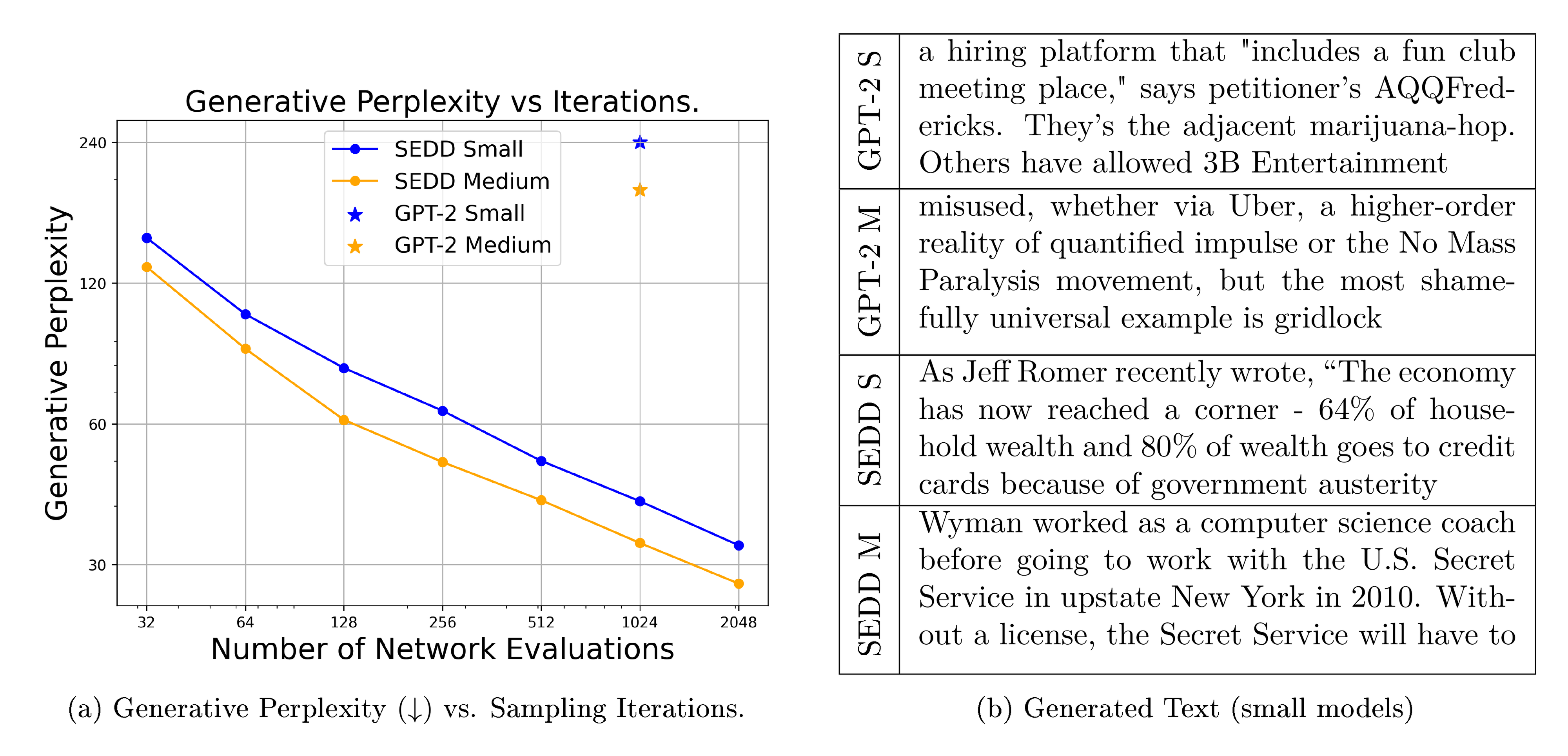
We first compare the quality of unconditional samples between GPT-2 and SEDD. As most language metrics are meant for comparing conditional generations ([16]), we instead measure the generative perplexity of sampled sequences (using a GPT-2 large model for evaluation). This is a simple and common metric ([36, 37]) but can easily be "hacked" by simple distribution annealing methods. So, we compare analytically sampled generations (i.e. no temperature scaling).

For SEDD, we simulate using 32 to 2048 steps, which approximates the learned distribution with minimal error for a large number of steps (the sequences are length 1024). Our results (both the measured generative perplexity and some samples) are shown in Figure 1. SEDD matches GPT-2 quality using 32 $\times$ fewer network evaluations and outperforms by $6$- $8\times$ when using the full 2048 steps. Furthermore, SEDD forms a predictable log-log linear pareto frontier between the number of sampling steps and generative perplexity. However, each network evaluation is different due to the KV-cache, which introduces a cost benefit tradeoff that we discuss more in Section 6.

:Table 4: Conditionally Generated Text. Prompt tokens are given in blue. Our model is able to generate meaningful text with prompt tokens in the front, the end, the middle, or even split up. Additional samples are given in Appendix D.3.

A bow and arrow is a traditional weapon that enables an attacker to attack targets at a range within a meter or maybe two meters. They have a range far longer than a human can walk, and they can be fired …
$\dots$ skydiving is a fun sport that makes me feel incredibly silly. I think I may’ve spent too much, but it could’ve been amazing! While sky diving gives us exercise and fun, scuba diving is an act of physical fitness, …
$\dots$ no one expected the results to much better than last year's one-sided endorsement. Nearly 90 percent of the results were surveyed as "independent, " an promising result for school children across the country.
$\dots$ results show that Donald Trump and Hillary Clinton are in 38 states combined with less than 1% of the national vote. In a way, it’s Trump and Hillary Clinton who will work overtime to get people to vote this $\dots$

5.3.2. INFILLING CONDITIONAL GENERATION

Finally, we showcase SEDD's ability for conditional generation. We generate samples conditioned on a fixed amount of input text (from the WebText dataset) and compare their MAUVE scores ([16]). For SEDD, we consider two prompting strategies: standard generation given the beginning and infilling using the beginning and end, although obviously more sampling strategies exist (and several are visualized in Table 4).

We compare against GPT-2 and SSD-LM ([36]), a competitive language diffusion model built for this task (all models are medium sized). Interestingly, a critical component for both baselines is distribution annealing: nucleus sampling for autoregressive modeling ([6]) (which clips the token probability) and thresholding for diffusion ([10, 38]) (which constrains generation to disallow paths in low probability spaces). As introducing similar annealing methods for SEDD is out of scope for this paper, we compare against both the annealed and un-annealed baselines samples.

Our results are given in Table 5. SEDD is highly competitive with the best configuration for both baselines, in fact beating both when using standard prompting. This is rather notable since SEDD does not use distribution annealing and does not explicitly encode left to right prompting as an architectural inductive bias (while GPT-2 and SSD-LM were trained explicitly for autoregressive-like generation).

:Table 5: Evaluation of conditionally generated text. SEDD with standard prompting beats both GPT-2 and SSD-LM. SEDD also offers more flexibility (enabling infilling generation with comparable performance) and does not require distribution annealing techniques for good generation.

Method	Annealing	Mauve ($\uparrow$)
GPT-2	Nucleus-0.95	0.955
	None	0.802
SSD-LM	Logit Threshold-0.95	0.919
	None	0.312
SEDD Standard	None	0.957
SEDD Infill	None	0.942

6. Related Work

Section Summary: This section reviews prior research on diffusion models for text, starting with continuous versions that embed words in a hidden space for gradual noise addition and removal, which have improved through better training techniques and can nearly match traditional word-by-word generation models. Discrete diffusion models, which work directly with word sequences, have shown promise for tasks like translation and faster processing but have faced hurdles in language applications compared to image use. The proposed SEDD method advances discrete diffusion by using a more reliable scoring approach that outperforms earlier versions and even some continuous models on text quality and efficiency, while challenging standard generation models like GPT-2 and offering potential for larger batches without memory trade-offs in sampling.

Continuous Diffusion Models for Text Data. Initially proposed by [10], continuous language diffusion models embed tokens in a latent space, learn a diffusion model there, and take the nearest neighbor to dequantize. While initial versions struggled, these models have achieved significant results by iterating on several empirical components. For example, prior works improve downstream performance with alternative loss functions (moving away from likelihood-based score matching) ([36, 39]) and explicitly encoding conditional information (e.g. inputting an infilling mask) ([40, 37]). Additionally, distribution annealing methods like thresholding ([10]) and classifier-free guidance ([41]) can further improve generation quality, although recent work has shown that methods like self-conditioning ([42]) and designing a less sparse embedding space (e.g. based on bits) ([43]) can obviate the need for such methods. Finally, [14] showed that, with many surgical changes to the training paradigm, it is possible for language diffusion models to begin approaching autoregressive performance for likelihoods.

Discrete Diffusion Models. Most discrete diffusion works follow the framework set out by D3PM ([11]) which mimics "mean prediction" ([8]). These discrete diffusion methods are largely applied to fields other than language (e.g. images), likely due to empirical challenges. Despite this, some works have shown strong performance on language, particularly for seq-to-seq tasks and more efficient generation ([44, 45, 46]). Notably, from these works discrete diffusion has tended to be advantageous over continuous diffusion in reducing network evaluations.

SEDD vs Prior Work. SEDD is a discrete diffusion model that focuses on score matching, the crucial ingredient for continuous diffusions ([13, 8]). Many such works also focus on reversing a discrete diffusion process ([17, 28, 20]), so score entropy is naturally related with prior training objectives. However, SEDD focuses on a principled, scalable, and performant objective (namely denoising score entropy), filling in shortcomings found in previous works. In particular, prior methods train either with the equivalent of implicit score entropy (which is intractable and high variance) or propose alternate losses that suffer from other issues. These critical differences enable large improvements for language tasks, where prior discrete diffusion models have conspicuously struggled on.

Furthermore, SEDD achieves better results (for both perplexity and generation) than even continuous diffusion models (without resorting to empirically driven heuristics). This is desirable since discrete data should necessitate a novel approach. Future work could adapt empirical designs from continuous diffusion, further improving performance.

Finally, SEDD challenges autoregressive models, achieving competitive perplexities (beating GPT-2) and generation quality (beating nucleus sampling). While there is still a large gap with modern large language models, we believe that future work can bridge this using SEDD as a backbone.

SEDD vs Autoregressive Sampling Iterations. SEDD and autoregressive models have significantly different sampling procedures due to the introduction of the KV-cache for standard decoder-only transformer models. In particular, this complicates the inference code (as each network pass changes from being a standard full batch forward) and trades off speed with memory. For example, for our (known) unoptimized codebase and the existing huggingface transformers library ([47]), we observed that SEDD matches autoregressive inference time when using around 100 steps but can increase the batch size by roughly $4-6$ times by removing the KV-cache memory. Future work will likely decrease the steps required for optimal generation (similar to existing work in standard diffusion ([48])) which can improve this tradeoff.

7. Conclusion

Section Summary: Researchers have developed score entropy discrete diffusion, or SEDD, models, which are a type of discrete diffusion system that uses a specific scoring method and can be trained quickly with a new loss function called score entropy loss. These SEDD models outperform earlier language diffusion models and perform as well as traditional autoregressive models in terms of accuracy and output quality. The authors hope this approach will inspire future innovations that challenge the dominance of autoregressive methods in language modeling.

We have introduced score entropy discrete diffusion (SEDD) models, a discrete diffusion model that is parameterized by the concrete score and can be trained efficiently with our novel score entropy loss. SEDD beats previous language diffusion models and rivals autoregressive models for both perplexity and quality. We hope that future work can build off our framework to defines alternatives to the modern autoregressive language modeling paradigm.

Impact Statement

Section Summary: This paper outlines research that pushes forward the development of natural language generation, a technology for creating human-like text. While the field already faces ethical challenges such as bias, harmful content, and misinformation, this particular work introduces no new risks because it is mostly theoretical and operates on a small scale that doesn't create any real-world problems.

This paper proposes work that advances the field of natural language generation. Outside of existing ethical questions for this area (e.g. bias, toxicity, fake content), our approach does not present any specific danger as the core work is largely theoretical and not at the scale to pose a specific problem.

Acknowledgements

This project was supported by NSF (#1651565), ARO (W911NF-21-1-0125), ONR (N00014-23-1-2159), CZ Biohub, a Stanford HAI GCP grant. AL is supported by a NSF Graduate Research Fellowship.

Appendix

Section Summary: This appendix presents mathematical proofs for the paper's main results on optimizing loss functions in models handling categorical data. It demonstrates that a specific loss minimizes to zero when the model's score predictions match the ratio of data probabilities, using convexity and derivatives to show optimality. Additional proofs establish equivalences between expectations under different distributions, connections to denoising processes, and bounds on log-probabilities via KL divergences and path measures in stochastic differential equations.

A. Proof of Main Results

Proof of Prop 3.2. Given infinite samples, the loss becomes equivalent to minimizing

$ \min_\theta \sum_{x, y \neq x} p(x) w_{xy}\left(s_\theta(x)y - \frac{p(y)}{p(x)} \log s\theta(x)_y\right) $

where we have removed constants not depending on $\theta$. This is minimized when

$ s_\theta(x)y - \frac{p(y)}{p(x)} \log s\theta(x)_y $

is minimized for all $x, y$. Taking a derivative with respect to $s$ and setting to $0$, we see that this occurs when $s_\theta(x)_y = \frac{p(y)}{p(x)}$, which can be easily checked to be optimal as the function is convex as a function of $s$. One can check that the loss is $0$ at the minimum.

Proof of Prop 3.3. The trick is the categorical equivalent of the divergence theorem. In particular, we have

$ \begin{align*} \mathbb{E}{x \sim p} \sum{y \neq x} \frac{p(y)}{p(x)} f(x, y) &= \sum_{x, y: x \neq y} \frac{p(y)}{p(x)} p(x) f(x, y)\ &= \sum_{x, y: x \neq y} p(y) f(x, y)\ &= \mathbb{E}{y \sim p} \sum{x \neq y} f(x, y)\ &= \mathbb{E}{x \sim p} \sum{y \neq x} f(y, x) \end{align*} $

for abitrary $f$. By setting $f(x, y) = w_{xy} \log s_\theta(x)_y$, we get that

which is the desired equivalent (as the last term does not depend on $\theta$).

Proof of Thm 3.4. This is similar to the same denoising variant for concrete score matching. We just need to show that the $\log s_\theta(x_t)_y \frac{p_t(y)}{p_t(x)}$ marginalizes out, since everything else does not change or is a constant.

$ \begin{align*} \mathbb{E}{x \sim p} \sum{y \neq x} f(x, y) \frac{p(y)}{p(x)} &= \sum_{y \neq x} f(x, y) p_t(y)\ &= \sum_{y \neq x} \sum_{x_0} f(x_t, y) p(y | x_0) p_0(x_0)\ &= \mathbb{E}{x_0 \sim p_0} \sum{y \neq x} f(x, y) \frac{p(y | x_0)}{p(x | x_0)} p(x | x_0)\ &= \mathbb{E}{x_0 \sim p_0, x \sim p(\cdot | x_0)} \sum{y \neq x} f(x, y) \frac{p(y | x_0)}{p(x | x_0)} \end{align*} $

Applying this to our loss when $f(x, y) = w_{xy} \log s_\theta(x)_y$ gives us

$ \begin{align*} & \mathbb{E}{x \sim p} \left[\sum{y \neq x} w_{xy} \left(s_\theta(x)y - \frac{p(y)}{p(x)} \log s\theta(x)y + K\left(\frac{p(y)}{p(x)}\right)\right)\right] \ &= \mathbb{E}{x \sim p} \left[\sum_{y \neq x} w_{xy} \left(s_\theta(x)y + K\left(\frac{p(y)}{p(x)}\right)\right)\right] - \mathbb{E}{x_0 \sim p_0, x \sim p(\cdot | x_0)} \left[\sum_{y \neq x} \frac{p(y | x_0)}{p(x | x_0)} w_{xy} \log s_\theta(x)y\right]\ &= \mathbb{E}{x_0 \sim p_0, x \sim p(\cdot | x_0)} \left[w_{xy} \left(s_\theta(x)y \frac{p(y | x_0)}{p(x | x_0)} \log s\theta(x)_y + K\left(\frac{p(y)}{p(x)}\right)\right)\right] \end{align*} $

Proof of Thm 3.6. The full bound is given by

\log p_0^\theta(x_0) \le \mathcal{L}{\rm DWDSE}(x_0) + D{\rm KL}(p_{T | 0}(\cdot | x_0) \parallel \pi) $

where $\mathcal{L}_{\rm DWDSE}$ is given by

$ \int_0^T \mathbb{E}{x_t \sim p{t | 0}(\cdot | x_0)} \sum_{y \neq x_t} Q_t(x_t, y) \left(s_\theta(x_t, t)y - \frac{p{t | 0}(y | x_0)}{p_{t | 0}(x_t | x_0)} \log s_\theta(x, t)y + K\left(\frac{p{t | 0}(y | x_0)}{p_{t | 0}(x_t | x_0)}\right)\right) dt $

Effectively, $\mathcal{L}_{\rm DWSDE}$ is the path measure KL divergence ([17, 49]), and the proof follows similarly. In particular, we have that, by the data processing inequality

$ -\log p_0^\theta(x_0) = D_{\rm KL}(\delta_{x_0} \parallel p_0^\theta) \le D_{\rm KL}(\mathbb{P}_{x_0} \parallel \mathbb{P}^\theta) $

where $\mathbb{P}{x_0}$ is the path measure for the reverse of the noising process applied to $\delta{x_0}$ and $\mathbb{P}^\theta$ is the learned reverse process. Generally, we can replace $\delta_{x_0}$ with a more general data distribution $p_{\rm data}$, with the computation remaining the same. We have,

$ D_{\rm KL}(\mathbb{P}{x_0} \parallel \mathbb{P}^\theta) \le \mathbb{E}{x_T \sim p_{T | 0}(\cdot | x_0)} \left[D_{\rm KL}(\mathbb{P}{x_0}(\cdot | x_T) \parallel \mathbb{P}^\theta(\cdot | x_T))\right] + D{\rm KL}(p_{T | 0}(\cdot | x_0) \parallel \pi) $

We analyze the term $\mathbb{E}{x_T} D{\rm KL}(\mathbb{P}_{x_0}(\cdot | x_T) \parallel \mathbb{P}^\theta(\cdot | x_T))$, which we can compute by Dynkin's formula ([27, 17]), which, similar to Girsanov's Theorem for standard SDEs ([50]), allows one to compute the change in measure. In particular, by applying Theorem 7.1 of [27] with degenerate SDE coefficients, we find the expectation to be given explicitly by

$ \begin{align} \int_0^T \mathbb{E}{x_t \sim p{t | 0}(\cdot | x_0)} &\sum_{y \neq x_t} \overline{Q}t^\theta(y, x_t) - Q_t(y, x_t) \log(\overline{Q}t^\theta(x_t, y))\ &+ Q_t(y, x_t) \log Q_t(y, x_t) + Q_t(x_t, y) K\left(\frac{p{t | 0}(y | x_0)}{p{t | 0}(x_t | x_0)}\right)dt \end{align} $

Since our reverse rate matrices $\overline{Q}t^\theta$ are parameterized with $s\theta$, we can simplify the above to

$ \int_0^T \mathbb{E}{x_t \sim p{t | 0}(\cdot | x_0)} \sum_{y \neq x_t} Q_t(x_t, y) \left(s_\theta(x_t, t)y + K\left(\frac{p{t | 0}(y | x_0)}{p_{t | 0}(x_t | x_0)}\right)\right) - Q_t(y, x_t) \log s_\theta(y, t)_{x_t} dt $

To finalize, we simply note that the summation over $Q(y, x_t) \log(s_\theta(y, t)_{x_t})$ can be simplified with the (reverse of) the trick used for proving Proposition 2.

$ \begin{align} \mathbb{E}{x_t \sim p{t | 0}(\cdot | x_0)} \sum_{y \neq x_t} Q(y, x_t) \log s_\theta(y){x_t} &= \sum{x_t, y \neq x_t} p_{t | 0}(x_t | x_0) Q(y, x_t) \log s_\theta(y){x_t}\ &= \mathbb{E}{y \sim p_{t | 0}(\cdot | x_0)} \frac{p_{t | 0}(x_t | x_0)}{p_{t | 0}(y | x_0)} Q(y, x_t) \log s_\theta(y){x_t}\ &= \mathbb{E}{x_t \sim p_{t | 0}(\cdot | x_0)} \frac{p_{t | 0}(y | x_0)}{p_{t | 0}(x_t | x_0)} Q(x_t, y) \log s_\theta(x_t)_{y} \end{align} $

where the last line is just a permutation of the notation of $x_t$ and $y$. As such, we get the desired loss

Proof of Thm 4.1. This can be shown by Bayes' rule:

$ p_{0 | t}(x_0 | x_t) = \frac{p_{t | 0}(x_t | x_0) p_0(x_0)}{p_t(x_t)} = p_{t | 0}(x_t | x_0) \frac{p_0(x_0)}{p_t(x_t)} $

We have $p_0 = \exp(-\sigma Q) p_t$ and $p_{t | 0}(x_t | x_0) = \exp(\sigma Q)_{x_t, x_0}$, so the theorem follows.

Proof of Thm 4.2. Using our factorization assumption we get that

$ \begin{align} &D_{\rm KL}\left(p_{t - \Delta t | t}(\mathbf{x}{t - \Delta t} | \mathbf{x}t) \parallel p{t - \Delta t | t}^\theta(\mathbf{x}{t - \Delta t} | \mathbf{x}t)\right)\ &= -\sum{i = 1}^d \mathbb{E}{\mathbf{x}{t - \Delta t} \sim p_{t - \Delta t | t}(\mathbf{x}{t - \Delta t} | \mathbf{x}t)} \left[\log p{t - \Delta t | t}^\theta(x{t - \Delta t}^i | \mathbf{x}_t)\right] + C \end{align} $

where $C$ is a constant independent of $\theta$. We simply need to minimize the following cross entropy loss for each $i$

\mathbb{E}{\mathbf{x}{t - \Delta t} \sim p_{t - \Delta t | t}(\mathbf{x}{t - \Delta t} | \mathbf{x}t) \left[\log p{t - \Delta t | t}^\theta(x{t - \Delta t}^i | \mathbf{x}_t)\right]} $

Our $\tau$-leaping condition implies that our transition assumes no change in other dimensions, so in particular $p_{t - \Delta t}^i (x_{t - \Delta t}^i | \mathbf{x}t) = p{t - \Delta t | t}^\theta(x_t^1 \dots x_{t - \Delta t}^i \dots x_t^d| \mathbf{x}t)$. By the standard properties of cross entropy, this is minimized when $p{t - \Delta t | t}^\theta(x_t^1 \dots x_{t - \Delta t}^i \dots x_t^d| \mathbf{x}t) = p{t - \Delta t | t}(\mathbf{x}_{t - \Delta t} | \mathbf{x}_t)$. This equality follows directly from Thm 4.1.

B. Algorithms for Training and Inference

**Require:** Network $s_\theta$, noise schedule  $\sigma$ (total noise $\overline{\sigma}$), data distribution $p_{\rm data}$, token transition matrix $Q$, time $[0, T]$.
Sample $\mathbf{x}_0 \sim p_0$, $t \sim \mathcal{U}([0, T])$.
Construct $\mathbf{x}_t$ from $\mathbf{x}_0$. In particular, $x_t^i \sim p_{t | 0}(\cdot | x_0^i) = \exp(\overline{\sigma}(t) Q)_{x_0^i}$.
**if** Q is Absorb { **then**
  This is $e^{-\overline{\sigma}(t)} e_{x_0^i} + \left(1 - e^{-\overline{\sigma}(t)}\right) e_{\rm MASK}$
**else if** Q is Uniform { **then**
  This is $\frac{e^{\overline{\sigma}(t)} - 1}{n e^{\overline{\sigma}(t)}} \mathbb{1} + e^{-\overline{\sigma}(t)} e_{x_0^i}$
**end if**
Compute $\widehat{\mathcal{L}}_{DWDSE} = \sigma(t) \sum_{i = 1}^d \sum_{y = 1}^n (1 - \delta_{x_t^i}(y)) \left(s_\theta(\mathbf{x}_t, t)_{i, y} - \frac{p_{t | 0}(y | x_0^i)}{p_{t | 0}(x_t^i | x_0^i)} \log s_\theta(\mathbf{x}_t, t)_{i, y}\right)$.
Backpropagate $\nabla_\theta \widehat{\mathcal{L}}_{DWDSE}$. Run optimizer.

**Require:** Network $s_\theta$, noise schedule $\sigma$ (total noise $\overline{\sigma}$), token transition matrix $Q$, time $[0, T]$, step size $\Delta t$
Sample $\mathbf{x}_T \sim p_{\rm base}$ by  sampling each $x_T^i$ from the stationary distribution of $Q$.
$t \gets T$
**while** $t > 0$ { **do**
  **if** Using Euler **then**
    Construct transition densities $p^i(y | x_t^i) = \delta_{x_t^i}(y) + \Delta t Q_t^{\rm tok}(x_t^i, y) s_\theta(\mathbf{x}_t, t)_{i, y}$.
  **else if** Using Tweedie Denoising **then**
    Construct transition densities $p^i(y | x_t^i) = \big(\exp(\overline{\sigma}(t - \Delta t) - \overline{\sigma}(t)) Q) s_\theta(\mathbf{x}_t, t)_i\big)_{y} \exp((\overline{\sigma}(t) - \overline{\sigma}(t - \Delta t)) Q)(x_t^i, y)$
  **end if**
  Normalize $p^i(\cdot | x_t^i)$ (clamp the values to be minimum $0$ and renormalize the sum to $1$ if needed).
  Sample $x_{t - \Delta t}^i \sim p^i(y | x_t^i)$ for all $i$, constructing $\mathbf{x}_{t - \Delta t}$ from $x_{t - \Delta t}^i$.
  $t \gets t - \Delta t$
**end while**
**Return:** $\mathbf{x}_0$

**Require:** A sampling algorithm (given above). Prompt spaces $\Omega$ and tokens $\mathcal{T}$.
$\mathbf{x}_T \sim p_{\rm base}$ as above. Set all indices in $\Omega$ to corresponding token in $\mathcal{T}$
$t \gets T$
**while** $t > 0$ { **do**
  Use prior methods to construct transition densities $p^i(y | x_t^i)$ for all $i$
  Sample $x_{t - \Delta t}^i \sim p^i(y | x_t^i)$ for all $i$ only if $i \notin \Omega$. Otherwise, set $x_{t - \Delta t}^i \gets x_t^i$ for $i \in \Omega$. Construct $\mathbf{x}_{t - \Delta t}$ from $x_{t - \Delta t}^i$.
  $t \gets t - \Delta t$
**end while**
**Return:** $\mathbf{x}_0$

C. Additional Experimental Details

C.1. Diffusion Details

The geometric noise distribution is $\overline{\sigma}(t) = \sigma_{\rm min}^{1 - t} \sigma_{\rm max}^t$. The log linear noise schedule is $\overline{\sigma}(t) = -\log(1 - (1 - \epsilon t))$ for some small epsilon for numerical stability as $t \to 1$, commonly $10^{-3}$ or $10^{-4}$. These noise schedules were chosen such that the prior loss $D_{\rm KL}(p_{T | 0}(\cdot x_0) \parallel \pi)$ and the approximation of $p_{\rm data}$ with $p_{\rm \overline{\sigma}(0)}$ are negligible. We typically scale the uniform transition matrix down by $\frac{1}{N}$ and take $p_{\rm base}$ to be uniform. For the absorbing state, we take $p_{\rm base}$ to be the MASK state with some leakage of probability to a random non-MASK state (to avoid $\inf$ KL divergence, although this is negligible and is not used for generation in practice).

C.2. Model Details

Our model train with flash attention ([51]) with fused kernels wherever applicable. We also use the adaLN-zero time information network of ([32]) with $128$ hidden dimension. Following previous work, we parameterize the network with the total noise level instead of the time $t$. We also found it easier to postprocess the output of our network to form $s_\theta$, rather than outputting it directly. Concretely, we exponentiate (which maintains positivity) to be beneficial to avoid numerical errors and also found that scaling by $e^{\overline{\sigma}} - 1$ helps for absorbing diffusion.

SEDD models have the same hidden dimensions, number of blocks, and number of heads as their corresponding GPT-2 models. However, SEDD models also use a separate word embedding matrix and output matrix. In total, SEDD small and SEDD medium have around 90M parameters and 320M non embedding parameters respectively (compared to GPT-2 small 86M and GPT-2 medium 304M non-embedding parameters respectively).

C.3. Training Details

All models were trained with a batch size of 512 and trained with a learning rate of $3 \times 10^{-4}$. We clip our gradient norm to 1 and have a linear warmup schedule for the first 2000 iterations. We also use a 0.9999 EMA.

We trained on nodes of 8 A100 80GB or 16 A100 40GB GPUs, using gradient accumulation when our batch size did not fit into memory (as is the case for SEDD medium).

C.4. Hyperparameter Search

We did not do a hyperparameter or achitecture search. Our hyperparameters were chosen for convenience purposes (e.g. the architecture was taken from DDiT ([32]), but we use rotary embeddings since they come included in previous work ([14])) or were naturally lifted from previous training recipes (e.g. the ubiquitous $3 \times 10^{-4}$ learning rate, $0.9999$ EMA).

C.5. Baseline Details (for Likelihood-based Training and Evaluation)

C.5.1. TEXT8

The baselines are taken from [52], with many coming from [11]. In particular, they are IAF/SCF ([53]), the Autoregressive Argmax Flow ([54]), and the discrete flow ([34]) for autoregressive models. The non-autoregressive baselines are, in order, Multinomial Diffusion ([54]), MAC ([55]), Bayesian Flow Networks ([52]), and D3PM ([11]).

C.5.2. ONE BILLION WORDS PERPLEXITY

The baselines are taken from [15]. They are D3PM ([11]), Diffusion-LM ([10]), BERT-mouth ([56]), and DiffusionBert ([15]).

C.5.3. GPT-2

The only two non GPT-2 baselines are PLAID ([14]) and D3PM (with Absorbing Transition) ([11]). We retrain both models (as they have not been trained with our exact specifications) to compare against small models. We reuse our model architecture and match hyperparameters (i.e. model size, training specifications).

C.6. Likelihood Evaluation Details

We randomly sample with $1000$ timesteps to Monte Carlo estimate our likelihoods. We use invertible tokenizers, as is customary for GPT-2 experiments. We report results on the test set for all datasets besides WikiText02, where we report on the train set since WikiText02 and WikiText103 share the same test set.

C.7. Unconditional Generation Details

We generate using the Tweedie denoiser, which performed slightly better than the Euler sampling (typically by 1-4 perplexity points). We generated $1000$ samples for all models.

C.8. Conditional Generation Details

We follow [36] and generate $5$ samples for each ground truth sample before calculating MAUVE. Note that this implies that we compare $5000$ generated samples and $1000$ ground truth samples. We sample by conditioning on $50$ tokens and generating a new $50$. For autoregressive-type sampling, this means we take the first $50$ tokens. For SEDD with infilling, this means we clamp all input text sizes to a max of $100$ tokens and condition on the first and last $25$ tokens.

D. Additional Experimental Results

D.1. Ablation of Concrete Score Matching

We also ablated the concrete score matching objective from ([57]) for the GPT-2 scale experiments. This was done by simply replacing the score entropy term with the corresponding $\ell^2$ based loss (in particular keeping the scaling by $Q_t(x, y)$). In general, we found that this did not train well, resulting in $3-4\times$ higher likelihood loss, which corresponds to 10, 000 $\times$ higher perplexity. Similarly,

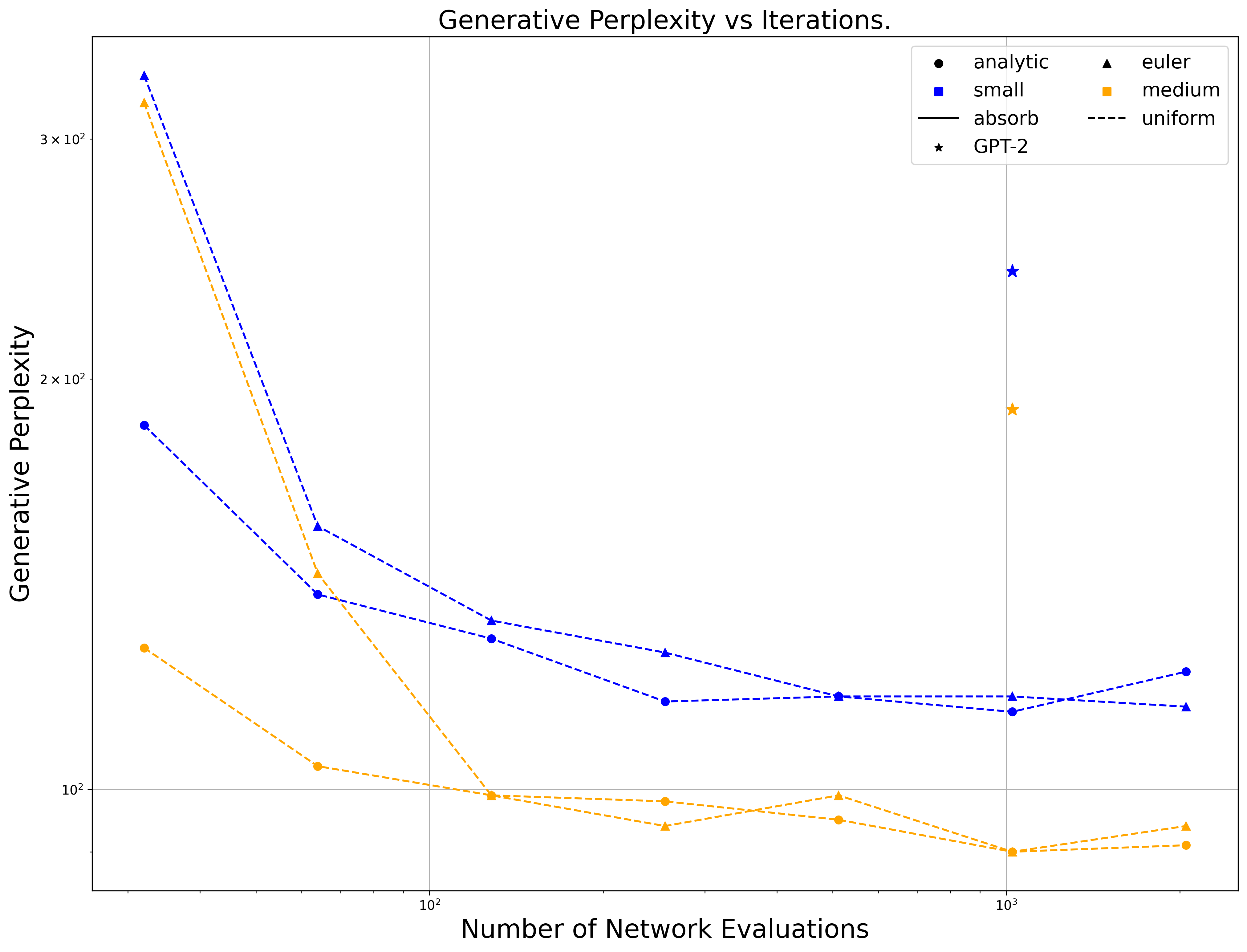
**Figure 2:** Generative Perplexity for SEDD Uniform.

D.2. Further Evaluation of Generative Perplexity

We further evaluate our generative perplexity for uniform models as well as different sampling schemes (analytic sampling based on Tweedie's vs Euler sampling based off of reverse diffusion). Results are shown in Figure 2. Generally, we find that uniform does not produce the same linear tradeoff curve as absorbing (most likely due to a bottleneck in generation quality). Futhermore, analytic generally outperforms Euler sampling, and this is a major factor for the uniform model.

We also generated on our trained baselines ([11, 14]), finding both performed substantially worse than our SEDD Absorb baseline but slightly better than our SEDD Uniform.

D.3. Additional Samples

Continued on next page.

**Figure 3:** GPT-2 Small Analytic Sampling. Unconditional

**Figure 4:** SEDD-Uniform Small. Unconditional

**Figure 5:** SEDD-Absorbing Small. Unconditional

**Figure 6:** GPT-2 Medium Analytic Sampling. Unconditional.

**Figure 7:** SEDD-Uniform Medium. Unconditional

**Figure 8:** SEDD-Absorbing Medium. Unconditional

**Figure 9:** SEDD-Absorbing Small. Conditional in blue.

**Figure 10:** SEDD-Absorbing Small. Conditional in blue.

**Figure 11:** SEDD-Absorbing Small. Conditional in blue.

**Figure 12:** SEDD-Absorbing Medium. Conditional in blue.

**Figure 13:** SEDD-Absorbing Medium. Conditional in blue.

**Figure 14:** SEDD-Absorbing Medium. Conditional in blue.

References

Section Summary: This references section provides a bibliography of key academic papers and books that support the research, drawing from fields like artificial intelligence and machine learning. It features influential works on generating images and text through methods such as language models, diffusion processes, and attention mechanisms, with contributions from researchers at organizations like OpenAI and Google. The citations range from foundational studies on statistical patterns and neural networks in the early 2000s to recent 2023 papers on advanced generative modeling techniques.

[1] Ramesh, A., Dhariwal, P., Nichol, A., Chu, C., and Chen, M. Hierarchical text-conditional image generation with clip latents. ArXiv, abs/2204.06125, 2022. URL https://api.semanticscholar.org/CorpusID:248097655.

[2] Brown, T., Mann, B., Ryder, N., Subbiah, M., Kaplan, J. D., Dhariwal, P., Neelakantan, A., Shyam, P., Sastry, G., Askell, A., Agarwal, S., Herbert-Voss, A., Krueger, G., Henighan, T., Child, R., Ramesh, A., Ziegler, D., Wu, J., Winter, C., Hesse, C., Chen, M., Sigler, E., Litwin, M., Gray, S., Chess, B., Clark, J., Berner, C., McCandlish, S., Radford, A., Sutskever, I., and Amodei, D. Language models are few-shot learners. In Advances in Neural Information Processing Systems, volume 33, 2020.

[3] Yule, G. U. On a method of investigating periodicities in disturbed series with special reference to wolfer’s sunspot numbers. Statistical Papers of George Udny Yule, pp.\ 389–420, 1971.

[4] Vaswani, A., Shazeer, N. M., Parmar, N., Uszkoreit, J., Jones, L., Gomez, A. N., Kaiser, L., and Polosukhin, I. Attention is all you need. In NIPS, 2017.

[5] Radford, A., Wu, J., Child, R., Luan, D., Amodei, D., and Sutskever, I. Language models are unsupervised multitask learners. 2019. URL https://api.semanticscholar.org/CorpusID:160025533.

[6] Holtzman, A., Buys, J., Du, L., Forbes, M., and Choi, Y. The curious case of neural text degeneration. In International Conference on Learning Representations, 2019.

[7] Sohl-Dickstein, J., Weiss, E., Maheswaranathan, N., and Ganguli, S. Deep unsupervised learning using nonequilibrium thermodynamics. In Proceedings of the 32nd International Conference on Machine Learning, 2015.

[8] Ho, J., Jain, A., and Abbeel, P. Denoising diffusion probabilistic models. In Advances in Neural Information Processing Systems, 2020.

[9] Song, Y., Sohl-Dickstein, J., Kingma, D. P., Kumar, A., Ermon, S., and Poole, B. Score-based generative modeling through stochastic differential equations. In International Conference on Learning Representations, 2021c. URL https://openreview.net/forum?id=PxTIG12RRHS.

[10] Li, X., Thickstun, J., Gulrajani, I., Liang, P. S., and Hashimoto, T. B. Diffusion-lm improves controllable text generation. In Advances in Neural Information Processing Systems, 2022.

[11] Austin, J., Johnson, D. D., Ho, J., Tarlow, D., and van den Berg, R. Structured denoising diffusion models in discrete state-spaces. In Advances in Neural Information Processing Systems, 2021.

[12] Hyvärinen, A. Estimation of non-normalized statistical models by score matching. J. Mach. Learn. Res., 6:695–709, 2005.

[13] Song, Y. and Ermon, S. Generative modeling by estimating gradients of the data distribution. In Neural Information Processing Systems, 2019.

[14] Gulrajani, I. and Hashimoto, T. Likelihood-based diffusion language models. In Advances in Neural Information Processing Systems, 2023.

[15] He, Z., Sun, T., Wang, K., Huang, X., and Qiu, X. Diffusionbert: Improving generative masked language models with diffusion models. In Annual Meeting of the Association for Computational Linguistics, 2022.

[16] Pillutla, K., Swayamdipta, S., Zellers, R., Thickstun, J., Welleck, S., Choi, Y., and Harchaoui, Z. Mauve: Measuring the gap between neural text and human text using divergence frontiers. Advances in Neural Information Processing Systems, 34:4816–4828, 2021.

[17] Campbell, A., Benton, J., Bortoli, V. D., Rainforth, T., Deligiannidis, G., and Doucet, A. A continuous time framework for discrete denoising models. In Advances in Neural Information Processing Systems, 2022.

[18] Anderson, W. J. Continuous-time Markov chains: An applications-oriented approach. Springer Science & Business Media, 2012.

[19] Kelly, F. Reversibility and stochastic networks. 1980. URL https://api.semanticscholar.org/CorpusID:125211322.

[20] Sun, H., Yu, L., Dai, B., Schuurmans, D., and Dai, H. Score-based continuous-time discrete diffusion models. In The Eleventh International Conference on Learning Representations, 2023.

[21] Meng, C., Choi, K., Song, J., and Ermon, S. Concrete score matching: Generalized score matching for discrete data. In Advances in Neural Information Processing Systems, 2022.

[22] Hyvärinen, A. Some extensions of score matching. Comput. Stat. Data Anal., 51:2499–2512, 2007. URL https://api.semanticscholar.org/CorpusID:2352990.

[23] Chen, R. T. Q. and Duvenaud, D. K. Neural networks with cheap differential operators. In Neural Information Processing Systems, 2019.

[24] Hutchinson, M. F. A stochastic estimator of the trace of the influence matrix for laplacian smoothing splines. Communications in Statistics - Simulation and Computation, 18:1059–1076, 1989. URL https://api.semanticscholar.org/CorpusID:120969358.

[25] Song, Y., Garg, S., Shi, J., and Ermon, S. Sliced score matching: A scalable approach to density and score estimation. In Conference on Uncertainty in Artificial Intelligence, 2019.

[26] Vincent, P. A connection between score matching and denoising autoencoders. Neural Computation, 23:1661–1674, 2011.

[27] Hanson, F. B. Applied Stochastic Processes and Control for Jump-Diffusions: Modeling, Analysis and Computation. Society for Industrial and Applied Mathematics, Philadelphia, PA, 2007. doi:10.1137/1.9780898718638. URL https://epubs.siam.org/doi/abs/10.1137/1.9780898718638.

[28] Benton, J., Shi, Y., Bortoli, V. D., Deligiannidis, G., and Doucet, A. From denoising diffusions to denoising markov models. ArXiv, abs/2211.03595, 2022. URL https://api.semanticscholar.org/CorpusID:253384277.

[29] Devlin, J., Chang, M.-W., Lee, K., and Toutanova, K. BERT: Pre-training of deep bidirectional transformers for language understanding. In Proceedings of the 2019 Conference of the North American Chapter of the Association for Computational Linguistics: Human Language Technologies, Volume 1 (Long and Short Papers). Association for Computational Linguistics, 2019.

[30] Gillespie, D. T. Approximate accelerated stochastic simulation of chemically reacting systems. Journal of Chemical Physics, 115:1716–1733, 2001. URL https://api.semanticscholar.org/CorpusID:5109777.

[31] Efron, B. Tweedie’s formula and selection bias. Journal of the American Statistical Association, 106:1602 – 1614, 2011. URL https://api.semanticscholar.org/CorpusID:23284154.

[32] Peebles, W. S. and Xie, S. Scalable diffusion models with transformers. In International Conference on Computer Vision, 2023.

[33] Su, J., Lu, Y., Pan, S., Wen, B., and Liu, Y. Roformer: Enhanced transformer with rotary position embedding. ArXiv, abs/2104.09864, 2021.

[34] Tran, D., Vafa, K., Agrawal, K., Dinh, L., and Poole, B. Discrete flows: Invertible generative models of discrete data. Advances in Neural Information Processing Systems, 32, 2019.

[35] Gokaslan, A. and Cohen, V. Openwebtext corpus. http://Skylion007.github.io/OpenWebTextCorpus, 2019.

[36] Han, X., Kumar, S., and Tsvetkov, Y. Ssd-lm: Semi-autoregressive simplex-based diffusion language model for text generation and modular control. arXiv preprint arXiv:2210.17432, 2022.

[37] Dieleman, S., Sartran, L., Roshannai, A., Savinov, N., Ganin, Y., Richemond, P. H., Doucet, A., Strudel, R., Dyer, C., Durkan, C., Hawthorne, C., Leblond, R., Grathwohl, W., and Adler, J. Continuous diffusion for categorical data. ArXiv, abs/2211.15089, 2022.

[38] Lou, A. and Ermon, S. Reflected diffusion models. In International Conference on Machine Learning. PMLR, 2023.

[39] Mahabadi, R. K., Tae, J., Ivison, H., Henderson, J., Beltagy, I., Peters, M. E., and Cohan, A. Tess: Text-to-text self-conditioned simplex diffusion. arXiv preprint arXiv:2305.08379, 2023.

[40] Gong, S., Li, M., Feng, J., Wu, Z., and Kong, L. Diffuseq: Sequence to sequence text generation with diffusion models. In The Eleventh International Conference on Learning Representations, 2023.

[41] Ho, J. Classifier-free diffusion guidance. ArXiv, abs/2207.12598, 2022. URL https://api.semanticscholar.org/CorpusID:249145348.

[42] Strudel, R., Tallec, C., Altché, F., Du, Y., Ganin, Y., Mensch, A., Grathwohl, W. S., Savinov, N., Dieleman, S., Sifre, L., et al. Self-conditioned embedding diffusion for text generation. 2022.

[43] Chen, T., Zhang, R., and Hinton, G. Analog bits: Generating discrete data using diffusion models with self-conditioning. arXiv preprint arXiv:2208.04202, 2022.

[44] Zheng, L., Yuan, J., Yu, L., and Kong, L. A reparameterized discrete diffusion model for text generation. ArXiv, abs/2302.05737, 2023.

[45] Chen, Z., Yuan, H., Li, Y., Kou, Y., Zhang, J., and Gu, Q. Fast sampling via de-randomization for discrete diffusion models. arXiv preprint arXiv:2312.09193, 2023.

[46] Ye, J., Zheng, Z., Bao, Y., Qian, L., and Wang, M. Dinoiser: Diffused conditional sequence learning by manipulating noises. arXiv preprint arXiv:2302.10025, 2023.

[47] Wolf, T., Debut, L., Sanh, V., Chaumond, J., Delangue, C., Moi, A., Cistac, P., Rault, T., Louf, R., Funtowicz, M., Davison, J., Shleifer, S., von Platen, P., Ma, C., Jernite, Y., Plu, J., Xu, C., Le Scao, T., Gugger, S., Drame, M., Lhoest, Q., and Rush, A. Transformers: State-of-the-art natural language processing. In Liu, Q. and Schlangen, D. (eds.), Proceedings of the 2020 Conference on Empirical Methods in Natural Language Processing: System Demonstrations, pp.\ 38–45, Online, October 2020. Association for Computational Linguistics. doi:10.18653/v1/2020.emnlp-demos.6. URL https://aclanthology.org/2020.emnlp-demos.6.

[48] Song, J., Meng, C., and Ermon, S. Denoising diffusion implicit models. In International Conference on Learning Representations, 2021a. URL https://openreview.net/forum?id=St1giarCHLP.

[49] Song, Y., Durkan, C., Murray, I., and Ermon, S. Maximum likelihood training of score-based diffusion models. In Neural Information Processing Systems, 2021b.

[50] Øksendal, B. Stochastic differential equations : an introduction with applications. Journal of the American Statistical Association, 82:948, 1987.

[51] Dao, T., Fu, D. Y., Ermon, S., Rudra, A., and R'e, C. Flashattention: Fast and memory-efficient exact attention with io-awareness. In Neural Information Processing Systems, 2022.

[52] Graves, A., Srivastava, R. K., Atkinson, T., and Gomez, F. Bayesian flow networks. arXiv preprint arXiv:2308.07037, 2023.

[53] Ziegler, Z. and Rush, A. Latent normalizing flows for discrete sequences. In International Conference on Machine Learning, pp.\ 7673–7682. PMLR, 2019.

[54] Hoogeboom, E., Nielsen, D., Jaini, P., Forré, P., and Welling, M. Argmax flows and multinomial diffusion: Learning categorical distributions. Advances in Neural Information Processing Systems, 34:12454–12465, 2021.

[55] Shih, A., Sadigh, D., and Ermon, S. Training and inference on any-order autoregressive models the right way. Advances in Neural Information Processing Systems, 35:2762–2775, 2022.

[56] Wang, A. and Cho, K. Bert has a mouth, and it must speak: Bert as a markov random field language model. arXiv preprint arXiv:1902.04094, 2019.

[57] Meng, C., He, Y., Song, Y., Song, J., Wu, J., Zhu, J.-Y., and Ermon, S. Sdedit: Guided image synthesis and editing with stochastic differential equations. In International Conference on Learning Representations, 2021. URL https://api.semanticscholar.org/CorpusID:245704504.