Zero-shot World Models Are Developmentally Efficient Learners

Khai Loong Aw, Klemen Kotar, Wanhee Lee, Seungwoo Kim, Khaled Jedoui, Rahul Venkatesh, Lilian Naing Chen, Michael C. Frank, Daniel L.K. Yamins

Stanford University

Corresponding author: [email protected]

Abstract

Young children demonstrate early abilities to understand their physical world, estimating depth, motion, object coherence, interactions, and many other aspects of physical scene understanding. Children are both data-efficient and flexible cognitive systems, creating competence despite extremely limited training data, while generalizing to myriad untrained tasks — a major challenge even for today's best AI systems. Here we introduce a novel computational hypothesis for these abilities, the Zero-shot Visual World Model (ZWM). ZWM is based on three principles: a sparse temporally-factored predictor that decouples appearance from dynamics; zero-shot estimation through approximate causal inference; and composition of inferences to build more complex abilities. We show that ZWM can be learned from the first-person experience of a single child, rapidly generating competence across multiple physical understanding benchmarks. It also broadly recapitulates behavioral signatures of child development and builds brain-like internal representations. Our work presents a blueprint for efficient and flexible learning from human-scale data, advancing both a computational account for children's early physical understanding and a path toward data-efficient AI systems.

Executive Summary: Young children quickly grasp the physical world—tracking motion, estimating depths, recognizing objects, and predicting interactions—despite limited experiences, a feat that stumps modern AI systems requiring vast labeled data. This gap hinders AI progress in areas like robotics and autonomous systems, while also posing puzzles for cognitive science about how human learning bootstraps such flexibility. The urgency stems from AI's growing role in real-world applications, where data efficiency could cut costs, improve safety, and enable deployment in low-resource settings like healthcare or child monitoring.

This document introduces the Zero-shot World Model (ZWM), a computational framework to explain and replicate children's efficient visual learning. It aims to demonstrate that a single, label-free model trained on a child's everyday videos can zero-shot perform diverse visual tasks, mirroring human development and advancing data-efficient AI.

Researchers trained ZWM, a neural network based on vision transformers, on egocentric video pairs from the BabyView dataset—head-camera footage from 34 infants aged 5 months to 3 years, totaling 868 hours of natural activities. The model predicts the second frame from the first plus sparse masked patches, forcing it to separate static appearances from motions without labels. They tested zero-shot extraction of abilities like optical flow (motion tracking) and object segmentation via simple perturbations, such as hypothetical movements, on standard benchmarks over 150-450 millisecond intervals. Comparisons included self-supervised baselines like DINOv3 and V-JEPA2, plus task-specific models trained on millions of labeled examples. Training used subsets like 132 hours from one child or age-ordered streams to probe efficiency and lifelong learning.

Key findings highlight ZWM's prowess. First, BabyZWM—trained solely on child videos—matches or exceeds state-of-the-art supervised models on optical flow accuracy (e.g., 80-90% pixel-level matching on real-world videos with occlusions) and occlusion detection. Second, it achieves over 90% accuracy in relative depth estimation from stereo views, outperforming large vision-language models like GPT-4 and rivaling supervised depth estimators. Third, on object discovery, it nears supervised segmenters trained on vast datasets, identifying bounded entities without prior categories. Fourth, in intuitive physics, it scores near 100% on reasoning about cohesion, support, force transfer, and separation in hand-object interactions. Finally, even on single-child data, performance holds steady, and developmental curves—tracking skill emergence over training—parallel infants' timelines, from early motion tracking to later physics grasp. Internal representations also align closely with human fMRI and monkey neural data, showing hierarchical buildup akin to brain maturation.

These results imply that structured prediction can unlock broad visual cognition from minimal, naturalistic data, challenging AI's reliance on massive labels and echoing a hybrid of innate priors (like temporal factoring) with learned content. For AI, this reduces risks from overfitting and cuts training costs by 10-100 times in data-poor fields like embodied robotics, where ZWM could enable safer action forecasting. In cognitive science, it supports empiricist views over strong nativism, as the model builds object and physics knowledge from experience alone, differing from prior work needing task-tuned heads. The brain-like hierarchies suggest ZWM captures universal principles of visual processing across species.

Leaders should prioritize ZWM-like architectures for AI prototypes in vision-critical applications, starting with pilots in robotics to test zero-shot planning. Next steps include integrating audio and language from child data for semantic understanding, extending to multi-frame predictions for longer actions, and creating standardized human-AI benchmarks. Trade-offs: Simpler models (170 million parameters) suffice for efficiency but may lag giants on edge cases; scaling to billion-parameter versions boosts robustness at higher compute.

Limitations include focus on short timescales, ignoring longer-term planning or uncertainty (leading to blurry predictions), and omission of linguistic concepts. No direct infant experiments limit behavioral claims, though benchmark proxies and neural alignments build confidence. Overall, results are robust across datasets, warranting strong trust for core findings, but caution applies to untested domains like complex semantics.

The ZWM framework

Section Summary: The Zero-shot World Model (ZWM) is a framework for building efficient visual models that can understand and predict scene changes without needing specific training for each task, by separating how things look from how they move. At its heart is a predictor that learns to fill in masked parts of video frames, implicitly capturing object appearances from full views and motions from sparse clues, which allows it to act like a simple simulator of the world. By making tiny tweaks to inputs and comparing predictions, ZWM extracts useful information like object outlines or depth zero-shot, and chains these steps together to handle more complex ideas, such as predicting physical behaviors.

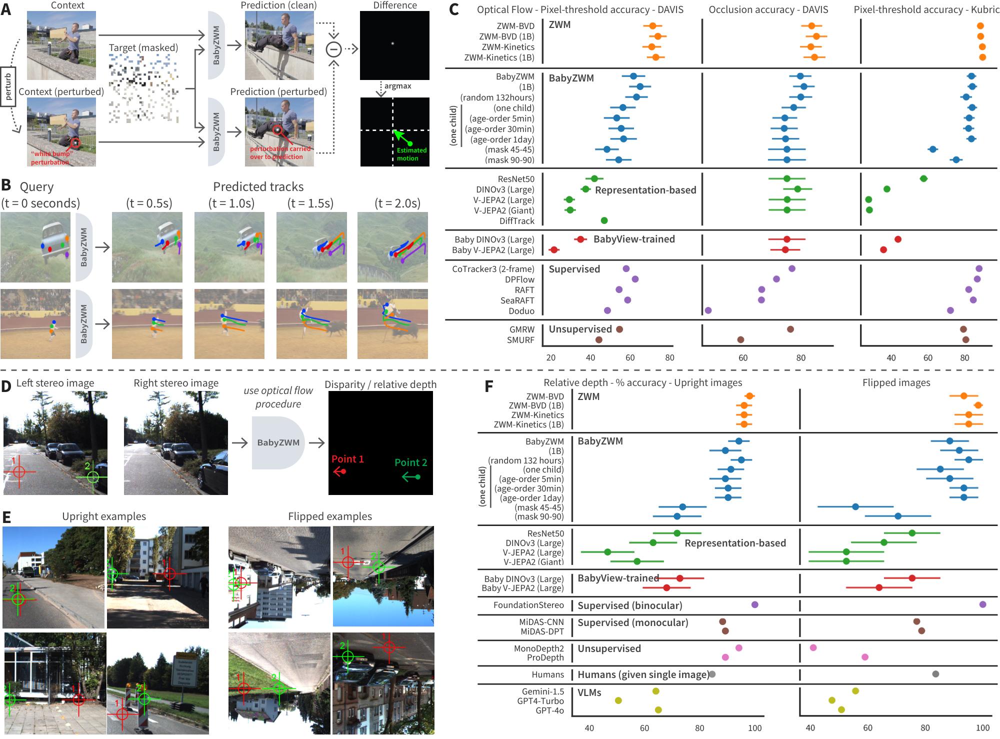
The Zero-shot World Model (ZWM) concept operationalizes our approach to data-efficient, zero-shot visual world modeling in three design principles ([@fig:main_framework] A): temporally-factored prediction to flexibly separate appearance from dynamics; zero-shot extraction of visual-cognitive structures from the predictor through approximate causal inference; and composing extractors together to achieve increasingly complex inference abilities. Taken together, the three components of ZWM form a kind of data-driven "world model" – so-called because the system can be used to forecast the effect of proxy actions (the probes) on a scene.

Sparse temporally-factored prediction.

The core learned component of the ZWM is a sparse temporally-factored masked multi-frame visual predictor, which we will denote by $\Psi$. Though the concept can be applied in longer-range many-frame videos (or even non-visual data domains), it is easiest to understand in the two-frame setting we use here ([@fig:main_framework] A). Given two RGB video frames $f_1$ and $f_2$ separated by a short time gap, let $\Psi_{\Theta}$ be a parameterized function that seeks to predict $f_2$ from $f_1$ together with a small fraction of pixel patches from $f_2$. The inputs to $\Psi_{\Theta}$ are thus of the form $(f_1, f_2^{\text{masked}})$, where $f_2^{\text{masked}}$ is a subset of the patches of $f_2$ after a mask has been applied. $\Psi_{\Theta}$ then outputs an estimate of the whole of $f_2$, denoted $\widehat{f}_2$. During training on ground truth frame pairs, the parameters $\Theta^*$ are optimized to minimize the average L2-loss of the prediction across the training dataset $\mathcal{D}$:

$ \Psi_{\Theta^*}: \left(f_1, f_2^{\text{masked}}\right) \longmapsto \widehat{f}2; \quad \quad \Theta^* := \arg \min{\Theta} \left \langle \lVert f_2 - \widehat{f}2 \rVert^{2}\right \rangle{(f_1, f_2) \in \mathcal{D}}. $

Two critical aspects of the training of $\Psi$ are that (i) the masks applied are very sparse – e.g. no more than 10% of the patches of $f_2$ are revealed; and (ii) training is performed with randomly-chosen masks, requiring no situation-specific knowledge of the semantic contents of the frames. $\Psi$ is a type of masked autoencoder [1, 2], in which the training mask is temporally biased to reveal all of one frame ($f_1$) and very little of the other ($f_2$). The constraints on this prediction problem are very generic – merely that masked training is performed, and that the masks are temporally biased. However, it turns out that this apparently weak generic constraint forces $\Psi$ to learn a very structured representation of the visual scene. Specifically, to successfully reconstruct $f_2$, $\Psi$ implicitly must: infer object appearance from the dense patches of $f_1$, as the small number of patches revealed from $f_2$ are insufficient to do so, while inferring object and camera motion transformations from the sparse revealed patches in $f_2^{\text{masked}}$. $\Psi$ thus implicitly factorizes appearance and motion, compressing low-dimensional motion data into a compact, but naturally interpretable, set of visual tokens.

Zero-shot extraction via approximate causal inference.

A key insight of ZWM is that the highly compressed but interpretable motion tokens that the training process creates can be manipulated with "zero-shot prompts" to extract key visual quantities by making the trained predictor's implicit knowledge explicitly available ([@fig:main_framework] A). The core mechanism of this process is to: (i) formulate a minimal perturbation of a ground-truth input; and (ii) compare the predictor $\Psi$ 's output in both the original ground-truth case and the minimally perturbed case, and (iii) aggregate the difference to hone in on the quantity of interest. Formally, this process can be represented as:

$ x_{\delta} := \textbf{perturb}(x); \quad \quad \delta \Psi := \textbf{compare}(\Psi(x), \Psi(x_{\delta})); \quad \quad \text{output} := \textbf{aggregate}(\delta \Psi). $

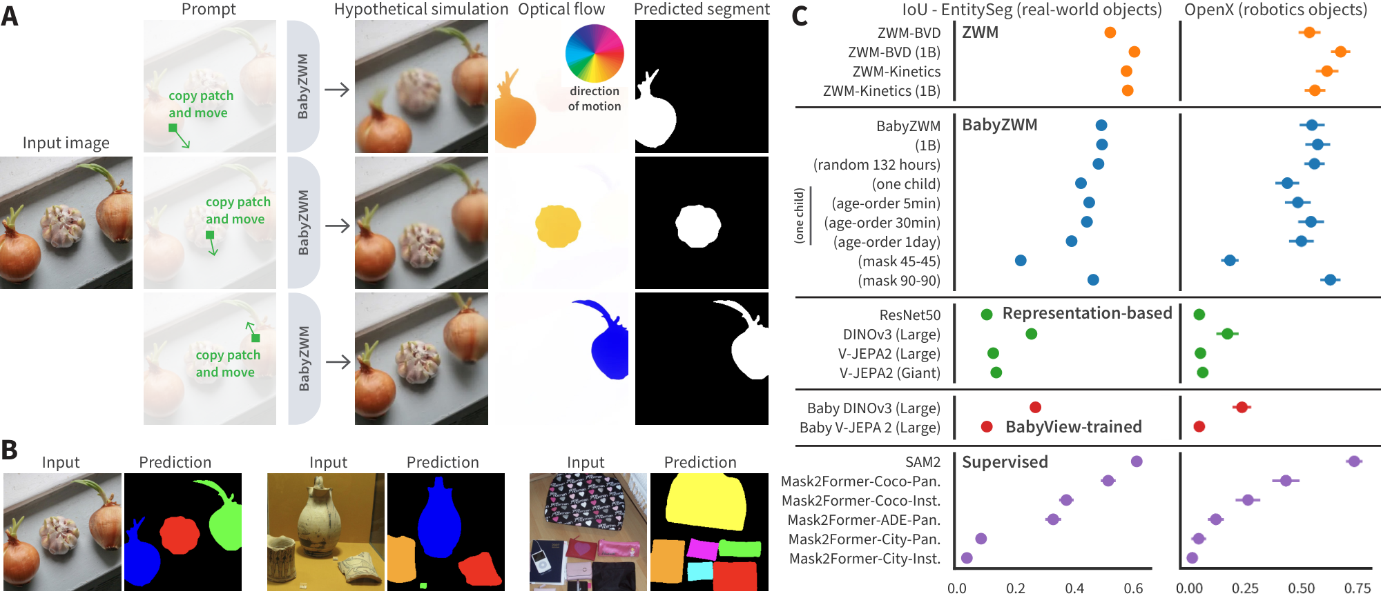
For example, to segment an object, the perturb function can simply induce hypothetical motion by translating one small patch on the object, causing the predictor $\Psi$ to propagate hypothetical motion to the rest of the object, but not other components in the scene; the compare function computes the optical flow between the perturbed and unperturbed cases; and aggregate thresholds the flow to determine which pixels belong to the object. We show that a wide variety of visual concepts can be extracted in a zero-shot manner from $\Psi$ by choosing different but extremely simple perturb, compare, and aggregate functions.

ZWM's approach to zero-shot extraction is a form of approximate causal inference. As discussed in the causality literature [3, 4], the process of causal inference asks how an outcome of a dynamic process changes when a minimal change is made to its antecedents. Analogously, the $\Psi$ function acts as a learned structural equation for the world's dynamics, whose temporally-factored nature permits the construction of minimal perturbations that expose some aspect of the causal structure of the world. For example, ZWM's object segmentation procedure uses a motion perturbation to expose the underlying causal structure of the world — groups of pixels move together due to the latent cause of belonging to the same physical object.

Compositional prompting.

ZWM composes simple prompts to construct more complex queries, progressively extracting and integrating increasingly abstract visual structures, e.g., motion and objects, rather than RGB pixels ([@fig:main_framework] A). ZWM (i) estimates optical flow from RGB; (ii) computes optical flow on binocular views for relative depth; (iii) simulates hypothetical motions and computes optical flow to segment objects; and (iv) uses flow and segments for intuitive physics. Consequently, this composition builds a computational graph of visual intermediates.

Model implementation.

We implement the predictor $\Psi$ as a neural network, and perform learning via stochastic gradient descent on its parameters. The base network architecture is a Vision Transformer (ViT) backbone [5], with versions at two sizes (170 million and 1 billion parameters). We compare models trained on a variety of datasets, as described below. In each case, training datapoints consist of RGB frame pairs taken from a real-world video distribution, with an inter-frame gap sampled uniformly between 150ms and 450ms. The images are input into the model as square 256x256 pixel arrays, and then patchified into 8x8-pixel patches. During training, masks are chosen randomly on each example, with 10% of patches in the second frame revealed.

Results

Section Summary: The ZWM model, trained on everyday video datasets like those mimicking a baby's view, excels at zero-shot visual-cognitive tasks such as estimating motion flow, judging relative depths, and identifying objects, performing as well as or better than many specialized computer vision systems without any task-specific training. When compared to standard image models like ResNet or video models like V-JEPA2, ZWM stands out by directly applying its learned world understanding without needing adjustments, while also matching or surpassing supervised benchmarks on challenging real-world videos. For instance, it achieves over 90% accuracy in depth estimation, rivals object segmentation tools trained on massive labeled data, and competes with top motion-tracking algorithms despite relying on far less diverse or labeled input.

ZWM performs diverse visual-cognitive tasks zero-shot

How well can ZWM flexibly perform a broad suite of visual-cognitive tasks zero-shot? We evaluate a spectrum of visual-cognitive tasks that humans perform, from lower- to higher-level, including optical flow, relative depth estimation, object segmentation, and intuitive physical reasoning. To test robustness across visual diets, we train ZWM on BabyView (N=34, 868 hours, 2025.1 release) [6] (BabyZWM), Kinetics-400 [7] ($\sim$ 670 hours) (smaller than BabyView but far more diverse Internet videos), and a Big Video Dataset (BVD) [8] ($\sim$ 7000 hours; computer vision datasets and Internet videos; an approximate upper bound on what can be achieved with high visual diversity and scale).

We evaluate ZWM against a range of alternative hypotheses, including both representation-based models and task-specific systems. Representation-based systems learn general-purpose visual features from pretraining that are typically transferred to downstream tasks via finetuning or lightweight task-specific heads/objectives. Unlike ZWM, these models are not natively zero-shot, a key limitation for modeling human vision, so we design simple zero-shot probes to evaluate these models. As a "standard" supervised static image model, we evaluate ResNet-50 trained on ImageNet-1k with category-label supervision. For a task-generic self-supervised static image model, we evaluate DINOv3 [9] (and DINOv3 trained on BabyView), which learns strong single-image representations by training the model to produce consistent features across different views of the same image, on BabyView. As an example of a task-generic self-supervised video model, we evaluate V-JEPA2 [10] (both as released and trained on BabyView), a model that learns by predicting masked regions of a video in feature space rather than in raw pixels.

Poor results across visual-cognitive tasks for these representation-based comparison models do not imply they do not develop useful and powerful visual-cognitive representations, but rather that these models provide no means of accessing these representations zero-shot. We therefore also benchmark ZWM against state-of-the-art task-specific baselines, including models trained directly for individual benchmarks (e.g., supervised networks optimized for flow, depth, or segmentation). These baselines can be viewed as concrete instantiations of the alternative hypothesis that human-like competence is achieved via separate, specialized systems rather than a unified world model. Due to the paucity of benchmarks for direct model-to-human comparisons, and because humans would be expected to perform near ceiling on these everyday visual tasks, we instead treat supervised state-of-the-art systems as a strong proxy baseline. Outperforming them therefore provides a strong test of BabyZWM’s zero-shot data efficiency.

We evaluate on established benchmarks designed to be challenging (real-world motion, occlusions, and lighting changes). For fair comparisons, we provide all models with the same inputs. We describe detailed methods for each task in the Supplementary Materials.

Optical flow.

To rigorously evaluate algorithm performance on optical flow, we use several recent computer vision benchmarks: TAP-Vid-DAVIS [11], consisting of challenging real-world videos with human-annotated "ground-truth"; and TAP-Vid-Kubric [12], consisting of synthetic, simulator-generated videos where ground-truth flows are known by construction. For each algorithm capable of producing flow predictions, we measure pixel-threshold accuracy (percentage of predictions within a pixel-radius of ground truth) and occlusion/out-of-frame detection accuracy. ZWM achieves state-of-the-art results (Figure 1 C); BabyZWM is competitive with label-supervised CoTracker3, DPFlow, and SeaRAFT [13, 14, 15] on TAP-Vid-DAVIS and matches supervised baselines at detecting occlusions. On TAP-Vid-Kubric, BabyZWM is strong but slightly below supervised models (which use synthetic training). BabyZWM outperforms the DINOv3 and V-JEPA2 models.

Relative depth estimation.

We evaluate depth perception on UniQA-3D [16]: point pairs that require judging which is further. Depth is extracted zero-shot from ZWM by computing optical flow between stereo images (Figure 1 D). Both ZWM and BabyZWM exceed 90% accuracy (Figure 1 F). They surpass large vision–language models (Gemini-1.5, GPT-4-Turbo, GPT-4o) [17, 18, 19], are comparable to supervised (MiDaS-CNN [20]) and self-supervised (MonoDepth2 [21]) monocular estimators, and trail only a supervised binocular model [22].

Object discovery.

We evaluate object segmentation on SpelkeBench [23], a class-agnostic benchmark defining objects as distinct, bounded entities. On this benchmark, BabyZWM rivals supervised Mask2Former variants [24] trained on large-scale COCO [25], though it performs slightly below SAM2 [26] which leverages large-scale human annotations (Figure 2 C).

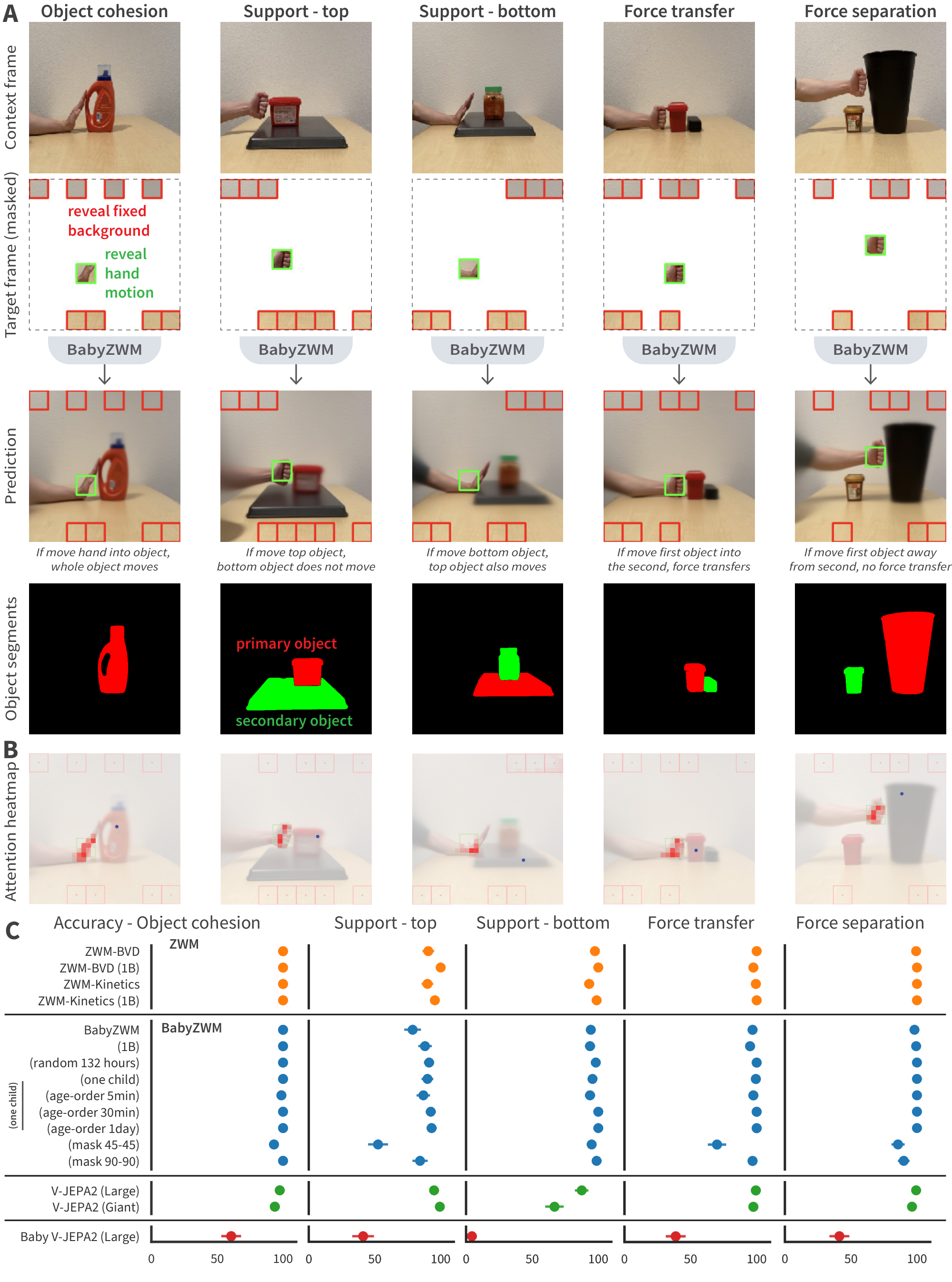
Intuitive physical understanding.

We develop a novel short-timescale physical reasoning benchmark (Figure 3 A) to evaluate models, featuring interactions between a hand and 1–2 objects that test 5 categories of reasoning: object cohesion, support relations with motion of either the top or bottom object, force transfer, and force separation. We define accuracy by comparing if the prediction is closer to the ground-truth target or the context, using mean squared error and LPIPS perceptual similarity [27]. ZWM, BabyZWM and V-JEPA2 all approach 100% performance across all categories, but not Baby V-JEPA2 (Figure 3 C). We apply model interpretability techniques to BabyZWM, revealing several attention heads that consistently follow the hand (causal agent) when predicting the motion of the object of interest (Figure 3 B).

ZWM achieves data efficiency and continual learning

A correct theory of visual-cognitive learning must be able to achieve effective learning on the real datastreams that a human experiences.

BabyZWM retains most of its performance compared to the same architecture trained on much more diverse datasets, such as Kinetics-400 and BVD (Figure 1, Figure 2, Figure 3), emphasizing the data-efficiency of the ZWM architecture.

To perform an even more stringent test, we next trained ZWM on Single-Child BabyView, a subset of BabyView consisting of 132 hours of recordings from a single individual (age 9–30 months). The Single-Child dataset represents a stricter test for model learning, because it requires algorithms to be able to learn generalizable capacities from the highly restricted visual diversity of one child's experience. (We additionally train on a random 132-hour subset, allowing us to disentangle the contributions of diversity versus total exposure.) Single-Child BabyZWM performs similarly to BabyZWM across most tasks (Figure 1, Figure 2, Figure 3).

Additionally, we trained a version of Single-Child BabyZWM on a single pass through a version of the data in which the video clips were ordered by the child's age. This is an important test of developmental robustness and continual/life-long learning. We create a set of curricula by shuffling within various temporal windows (5 minutes, 30 minutes, and 1 day), loosely approximating different degrees of experience consolidation (e.g., within-episode mixing vs. sleep-like reordering). The age-ordered Single-Child BabyZWM models performed similarly to Single-Child BabyZWM across all tasks (Figure 1, Figure 2, Figure 3).

Finally, "Standard" BabyZWM uses asymmetric masking (fully visible $f_1$, 90% masked $f_2$), explicitly prioritizing the learning of motion dynamics. Because this temporally-factored mask structure contributes a conceptually core component of the ZWM concept, we explore simpler alternatives. We evaluate symmetric masking variants of BabyZWM (mask 45%-45% and mask 90%-90%), which perform substantially worse (Figure 1, Figure 2), showing that emphasizing motion information is useful for data efficiency and zero-shot abstraction.

BabyZWM's developmental curves broadly parallel children's learning

Having evaluated the BabyZWM models, we next ask what we can learn from looking at their developmental trajectories and when different visual-cognitive capacities emerge. BabyZWM's optical flow accuracy increases across training, then plateaus, broadly paralleling children's single-/multi-object tracking development [29, 30] (Figure 4 A). Relative-depth estimation capacities increase steeply with training data and stay high (Figure 4 B), echoing early stereopsis [31, 32, 33] with continued development [34]. Object segmentation capabilities continue improving over training (Figure 4 C), echoing developmental findings that object perception/segmentation improves over infancy [35, 36]. Finally, intuitive physics capabilities improve over training (Figure 4 D), mirroring infants’ progression: early coarse expectations about cohesion, continuity, and solidity sharpen into precise support reasoning (e.g., center-of-mass), sensitivity to causal launching/force transfer, and refined occlusion/containment distinctions. These gains likely reflect the model learning increasingly rich priors about objects and their dynamics [37, 36, 38]. While these trajectory comparisons are intriguing, they should be interpreted cautiously. They partly reflect benchmark-specific design choices – especially differences in task difficulty, metrics, and ceiling effects – rather than a clean ordering of underlying capability development. Therefore, one takeaway is the need for more systematic, comparable benchmarking for early visual abilities in humans and machines.

ZWM representations align with neural responses

Having shown that ZWM exhibits human-like behavioral signatures, we next ask whether they also develop brain-like internal representations. The human visual system is organized hierarchically, transforming retinal inputs into increasingly complex representations [40, 41, 42] that develop over childhood [43, 44, 45, 46, 47]. We evaluate the similarity of our models' internal representations (across various training checkpoints) with brain responses by computing neural predictivity [48, 49, 50]: fit a cross-validated linear probe from model features to neural responses, then report noise-corrected correlations (Figure 5 A). We evaluate two complementary benchmarks: the Natural Scenes Dataset (NSD) [51] for human fMRI and the THINGS Ventral Stream Spiking Dataset (TVSD) [52] for macaque electrophysiology. fMRI captures large-scale representational geometry; electrophysiology reveals fine-grained single-neuron tuning/timing.

Across NSD and TVSD, the BabyZWM model exhibits neural alignment consistent with hierarchical visual development. Neural predictivity for early visual cortex approaches its noise ceiling at relatively early training checkpoints, whereas higher regions improve more gradually, an "early-first" developmental trajectory (Figure 5 B). Layer–area correspondence is hierarchically aligned: for earlier cortical regions, earlier model layers reach the noise ceiling, whereas later cortical regions align with deeper layers (Figure 5 C). This pattern is consistent with several accounts of hierarchical visual organization [40, 53, 41, 42] and prior modeling findings [48, 49], supporting an explicit "mechanistic mapping" between model layers and cortical regions [54, 55, 56]. A single, self-supervised world model thus captures representational structure shared across species and measurement scales, and BabyZWM recapitulates human-like signatures of both developmental dynamics and hierarchical organization.

Discussion

Section Summary: Modern visual learning algorithms struggle with data efficiency compared to humans, but a new approach called Zero-shot World Modeling (ZWM) bridges this gap by creating unified models that predict and understand visual scenes without needing task-specific labels, allowing generalization to real-world situations even from limited video data of a single child. This method eliminates the reliance on expensive labeled data in AI, similar to how large language models revolutionized natural language processing, and it blends ideas from pure machine learning with human-like cognitive priors to boost efficiency in areas like robotics and medical imaging. While ZWM excels at physical understanding early in development, it has limitations, such as not covering semantic concepts like object names and lacking detailed comparisons to child brain data.

Modern visual learning algorithms are highly data inefficient when compared to humans, experiencing substantial performance gaps when trained on the real datastreams experienced by human children [57, 58, 59, 60, 6]. Here, we describe a novel approach to visual learning, Zero-shot World Modeling, that is able to bridge this gap. To acquire diverse visual-cognitive capacities without labels, ZWM represents a shift from the dominant paradigm of representation learning with task-specific readouts to unified, zero-shot world models. In representation learning, each downstream task needs its own labeled readout [61, 62, 63, 64, 65, 66, 67, 10], limiting the range of feasible tasks and encouraging overfitting to sparse labels. In contrast, ZWM achieves zero-shot, out-of-distribution generalization to challenging real-world scenes, synthetic simulations, and flipped images. Moreover, ZWM gains competence even when trained with limited data from one individual child, presented in an online single-epoch fashion.

Beyond its implications for cognitive science, ZWM's zero-shot capability addresses a pressing challenge in AI. Current self-supervised visual models, despite learning rich representations, remain locked behind task-specific labeled readouts – an expensive and brittle dependency that limits practical deployment. ZWM eliminates this bottleneck: a single learned predictor yields optical flow, depth, segmentation, and physical reasoning zero-shot, through a universal interface. This mirrors the paradigm shift in NLP when LLMs replaced task-specific fine-tuned models – but ZWM achieves this in vision with orders of magnitude less data. That this is achievable from just hundreds of hours of a single child's naturalistic, uncurated video – rather than millions of hours of curated internet data – suggests that the right inductive structure can dramatically reduce the data requirements for broad visual competence. This has direct relevance for domains such as robotics, medical imaging, and embodied AI, where large-scale labeled data is unavailable.

ZWM is a natural hybrid between two polar concepts of the role of intermediate structure in cognition and learning. The first is a "pure learning" alternative, embodied by Richard Sutton's Bitter Lesson [68] – that complex hand-built inductive biases are unnecessary in formulating effective learning machines. The second is the idea, emanating from computational cognitive science, that human learning is best understood as embodying strong priors about the world, citing the sophistication and early emergence of infants’ object and physical knowledge [69, 70, 71, 72] and poverty-of-stimulus claims that children’s input is too noisy to support learning [73, 74]. The ZWM principles draw on both of these ideas, illustrating how explicit structure can be created within a minimally-biased learned network.

The fact that ZWM can implement this hybrid, and the observation that doing so leads to substantial gains in learning efficiency, has implications for the long-standing debate between developmental nativism and empiricism. Specifically, ZWM instantiates a hybrid innateness hypothesis where a small set of structural priors may be innate – architecture, learning algorithm, and task-specific readout programs (e.g., for flow, depth, segmentation) – while the representational content and network parameters are learned from experience. Importantly, our results provide proof-of-concept validation that this mechanism supports acquisition of visual-cognitive capacities and object- and physics-like representations from naturalistic visual experience, challenging strong nativist accounts that posit extensive innate biases for representational content and concepts.

Under this interpretation, zero-shot readouts may correspond to evolutionarily-specified, hard-wired neural circuits that map learned dynamics to visual-cognitive percepts. Future work can explore if they might alternatively be learned during development as flexible adapters, or constructed online as query-like cognitive inference routines over the learned predictor.

ZWM achieves zero-shot visual cognition by being a world model, which forecasts the consequences of actions. This concept has a long tradition within model-based reinforcement learning [75, 76] and model-predictive control [77, 78, 79, 80, 81, 82, 83, 84, 85]. It might at first seem odd that we discuss ZWM as a world model—after all, the inputs to $\Psi$ are just data, so where are the actions whose consequences are to be forecasted? ZWM is a "data-driven world model", in which expensive-to-obtain true action data is proxied by cheap data (e.g. pixel-patch) operations that approximate simple actions – the "tracers" and "motions" used to create hypotheticals for computing flow, object segments, etc. ZWM formally treats data patches in the same way that true action data would be, and reaps the reward of doing so, because training on raw data enables the underlying model to learn enough about the way the world works that it can competently perform hypotheticals. Future work could seek to learn an interactive policy for choosing such "actions", setting up comparisons to observed child hand and head motions captured in the BabyView dataset.

Our present work has a number of important limitations. First, by focusing on physically-grounded quantities that are learned by very young infants, ZWM leaves unaddressed how semantic concepts – e.g. named linguistic categories of objects, relationships, activities – arise developmentally. We hope that future work will integrate the world model learned by ZWM with the rich linguistic/auditory data experienced by children. Second, a core empirical limitation of the present work is the paucity of detailed developmental behavioral and neural comparisons. Such datasets are very challenging to produce and will require concerted collaborative efforts. Finally, as a deterministic regression model, ZWM's $\Psi$ predictor is subject to mode collapse, leading to blurry predictions in situations in which there is underlying uncertainty about how the future will resolve. This design limits our ability to study longer-horizon prediction and control; extending to multi-frame training, richer temporal memory, and long-horizon tasks is an important next step [8].

One of the most intriguing lines for future work will be to integrate the zero-shot task extractions from the ZWM model into the underlying predictor $\Psi$, so that $\Psi$ can be conditioned on, and make predictions of, these intermediate quantities. Recent work in world modeling has suggested a possible mechanism for this type of integration [8, 86, 87], creating a bootstrapping cycle in which every additional intermediate could contribute a learnable target for enriching the predictor, in turn enabling increasingly efficient learning and the identification of more sophisticated intermediates. Perhaps these or similar ideas might pave the way for even more flexible, data-efficient learning of visual abstractions.

Acknowledgments

Section Summary: The authors express thanks to several researchers, including Cameron Ellis, Hyowon Gweon, James McClelland, Cliona O'Doherty, and Alison Gopnik, for providing helpful feedback on the manuscript, and they acknowledge funding from various grants like those from the Simons Foundation, National Science Foundation, and Office of Naval Research, along with computing support from Stanford and Google teams. Key contributions include research design, data analysis, and writing by K.L.A., M.C.F., and D.L.K.Y., with model implementation by K.L.A., K.K., and W.L., and specialized analyses by S.K., K.J., L.N.C., and R.V. There are no competing interests, and the code for model training along with the datasets will be publicly released upon publication to allow others to reproduce the results.

We are very grateful to Cameron Ellis, Hyowon Gweon, James (Jay) McClelland, Cliona O'Doherty, and Alison Gopnik for helpful feedback on our manuscript.

Funding:

This work was supported by the following awards. D.L.K.Y.: Simons Foundation grant 543061, National Science Foundation CAREER grant 1844724, National Science Foundation Grant NCS-FR 2123963, Office of Naval Research grant S5122, ONR MURI 00010802, ONR MURI S5847, and ONR MURI 1141386 - 493027. We also thank the Stanford HAI, Stanford Data Sciences, Stanford Marlowe team, and the Google TPU Research Cloud team for computing support.

Author contributions:

K.L.A., M.C.F., and D.L.K.Y. designed research, analyzed data, and wrote the paper; K.L.A., K.K., and W.L. implemented and trained models; S.K. implemented optical flow algorithms and analyses; K.J. implemented neural predictivity algorithms and analyses; L.N.C. and R.V. implemented object segmentation algorithms and analyses.

Competing interests:

There are no competing interests to declare.

Data and materials availability:

We will release the code for model training and evaluation when the paper is published, to enable readers to reproduce our results. The datasets used for training our BabyZWM model will also be made publicly available.

Supplementary Materials for Zero-shot World Models Are Developmentally Efficient Learners

Section Summary: This section lists the authors of the supplementary materials for the research paper "Zero-shot World Models Are Developmentally Efficient Learners," which explores how AI systems can learn about the world efficiently, similar to child development. The contributors are Khai Loong Aw, Klemen Kotar, Wanhee Lee, Seungwoo Kim, Khaled Jedoui, Rahul Venkatesh, Lilian Naing Chen, Michael C. Frank, and Daniel L.K. Yamins. Khai Loong Aw is the corresponding author and can be contacted at [email protected] for further details.

Khai Loong Aw$^{\ast}$, Klemen Kotar, Wanhee Lee, Seungwoo Kim, Khaled Jedoui, Rahul Venkatesh, Lilian Naing Chen, Michael C. Frank, Daniel L.K. Yamins $^\ast$Corresponding author. Email: [email protected]

Methods

Section Summary: The ZWM model is a vision transformer that processes pairs of video frames, where the first frame is fully visible and divided into small patches, while the second frame has 90 percent of its patches hidden to train the system to predict motion and changes. It comes in two sizes with 170 million or 1 billion parameters and is trained on real-world videos from children's perspectives, like the BabyView dataset, using a simple error measure to improve predictions over 200,000 steps without extra data tweaks. Tests showed that this uneven masking between frames is key for the model's ability to handle visual tasks, as balanced masking led to poorer results.

Model architecture

The ZWM predictor $\Psi$ is implemented as a Vision Transformer (ViT) [5]. Input frames are resized to $256 \times 256$ pixels and divided into non-overlapping $8 \times 8$-pixel patches, yielding $32 \times 32 = 1024$ patch tokens per frame. We evaluate two model sizes:

• ZWM-170M: 24 transformer layers, 12 attention heads, embedding dimension 768, totaling $\sim$ 170 million parameters.
• ZWM-1B: 48 transformer layers, 16 attention heads, embedding dimension 1280, totaling $\sim$ 1 billion parameters.

Two-frame input tokenization.

Given a frame pair $(f_1, f_2)$, the first frame $f_1$ is fully patchified into 1024 tokens, each a flattened $8 \times 8 \times 3 = 192$-dimensional vector. The second frame $f_2$ is masked: only 10% of its patches (approximately 102 tokens) are revealed, with the remaining patches replaced by a shared learnable mask token. Both sets of tokens receive positional embeddings (learned, not sinusoidal) before being concatenated and fed into the transformer.

Masking strategy.

During training, the mask for $f_2$ is sampled uniformly at random on each example, with exactly 10% of patches revealed. This ensures the model encounters diverse masking patterns and cannot rely on fixed spatial positions. The asymmetric structure—fully visible $f_1$, 90% masked $f_2$ —is a core design choice that encourages temporal factorization of appearance and motion.

Symmetric masking ablation.

To test whether this asymmetry is necessary, we trained BabyZWM variants with symmetric masking policies:

• Symmetric 45%-45%: Both frames are masked at 45%, so each frame reveals 55% of patches.
• Symmetric 90%-90%: Both frames are masked at 90%, so each frame reveals only 10% of patches.

Both symmetric variants perform substantially worse across all zero-shot visual-cognitive tasks (Figure 1 and Figure 2), demonstrating that the temporally-biased mask structure—rather than masking per se—is critical for learning representations that support flexible zero-shot extraction.

Output and loss.

The model outputs a prediction $\widehat{f}_2$ for the full second frame, including all masked positions. The training objective is the mean squared error (MSE) between the predicted and ground-truth pixel values of $f_2$, computed over masked patches:

$ \mathcal{L} = \left\langle \lVert f_2 - \widehat{f}2 \rVert^{2} \right\rangle{(f_1, f_2) \in \mathcal{D}}. $

: Table 1: Model architecture configurations. Architectural hyperparameters for the two ZWM model sizes evaluated in this work.

	ZWM-170M	ZWM-1B
Transformer layers	24	48
Attention heads	12	16
Embedding dimension	768	1280
Patch size	$8 \times 8$	$8 \times 8$
Input resolution	$256 \times 256$	$256 \times 256$
Tokens per frame	1024	1024
Total parameters	$\sim$ 170M	$\sim$ 1B

Training procedure

Each ZWM model is trained for 200, 000 steps with a batch size of 512. As the videos are stored at 30 frames per second, this corresponds to $\sim$ 950 video hours, or roughly 95 days of waking experience assuming $\sim$ 10 awake hours per day for young children [28].

Training datapoints consist of RGB frame pairs sampled from real-world video, with the inter-frame temporal gap randomly and uniformly chosen in the range 150–450ms (corresponding to 5–14 frames at 30 fps).

Optimization.

We use AdamW with a peak learning rate of 3e-4, weight decay of 1e-1, and $(\beta_1, \beta_2) = (0.9, 0.95)$. The learning rate follows a cosine decay schedule with 2000 warmup steps. We use gradient clipping with a maximum norm of 1.0.

Data augmentation.

No data augmentation (e.g., random crops, color jitter, horizontal flips) is applied during training. The model is trained directly on raw RGB frame pairs.

Compute.

All models are trained using PyTorch with Distributed Data Parallel (DDP) and mixed-precision (bfloat16). The ZWM-170M model is trained on 4 nodes of 8 NVIDIA H100 GPUs each (32 GPUs total) for approximately 11 hours ($\sim$ 352 GPU-hours). The ZWM-1B model is trained on 8 nodes of 8 H100 GPUs each (64 GPUs total) for approximately 24 hours ($\sim$ 1, 536 GPU-hours).

: Table 2: Training hyperparameters. Training configuration shared across all ZWM models unless otherwise noted.

Hyperparameter	Value
Optimizer	AdamW
AdamW $(\beta_1, \beta_2)$	(0.9, 0.95)
Peak learning rate	3e-4
Weight decay	1e-1
LR schedule	Cosine decay
Warmup steps	2000
Batch size	512
Total training steps	200, 000
Inter-frame gap	150–450 ms
Patches revealed during training ($f_1$)	100%
Patches revealed during training ($f_2$)	10%

1.1 Training datasets

We train ZWM on a spectrum of visual diets to test data efficiency and robustness:

BabyView.

The BabyView dataset [6] consists of 868 hours, mostly longitudinal, egocentric video recordings from $N=34$ children aged $\sim$ 5 months to 3 years, and $\sim$ 100 hours from 3–5-year-olds recorded in a preschool setting. Videos are recorded using head-mounted cameras worn by the children during natural daily activities. We refer to the ZWM model trained on the full BabyView dataset as "BabyZWM." The raw BabyView videos, recorded by families in their homes, are typically several minutes in duration. We preprocess all videos by splitting them into 10-second clips, stored at 30 fps with the shorter spatial dimension resized to 256 pixels (the longer side scaled proportionally to preserve aspect ratio). During training, we randomly sample a $256 \times 256$ crop from each frame pair, with the same crop applied to both $f_1$ and $f_2$. No additional augmentations are applied.

Single-Child BabyView.

To test learning from even more restricted experience, we construct a subset of BabyView consisting of 132 hours of recordings from a single individual (child S00320001, aged 9-30 months). This represents the most stringent test of data efficiency, requiring the model to learn generalizable capacities from the highly restricted visual diversity of one child's experience.

Random 132-hour subset.

To disentangle the contributions of visual diversity from total exposure, we also train on a random 132-hour subset of BabyView, sampled uniformly across all 34 children. This subset matches the Single-Child dataset in total duration but contains substantially more environmental diversity.

Age-ordered curricula.

To test continual learning and robustness to catastrophic forgetting, we train Single-Child BabyZWM in an online, single-epoch fashion on the age-ordered video stream. We create curricula by shuffling within temporal windows of varying durations:

• 5-minute shuffle: 10-second clips are randomly shuffled within contiguous 5-minute windows, preserving the coarse temporal order while introducing local mixing (analogous to within-episode consolidation).
• 30-minute shuffle: 10-second clips are shuffled within 30-minute windows.
• 1-day shuffle: 10-second clips are shuffled within full recording days, loosely approximating overnight sleep-like reordering.

Kinetics-400.

Kinetics-400 [7] consists of $\sim$ 670 hours of 10-second video clips from YouTube, spanning 400 human action categories. This dataset is smaller than BabyView but contains substantially more environmental and semantic diversity due to its Internet-sourced content.

Big Video Dataset (BVD).

BVD [8] consists of $\sim$ 7, 000 hours of video drawn from a combination of computer vision datasets and Internet videos. This serves as an approximate upper bound on performance achievable with high visual diversity and scale.

: Table 3: Training dataset statistics. Summary of the video datasets used to train ZWM variants.

Dataset	Hours	Source	ZWM variant
BabyView	868	34 children, egocentric	BabyZWM
Single-Child BabyView	132	1 child, egocentric	Single-Child BabyZWM
Random 132h subset	132	34 children, egocentric	—
Kinetics-400	$\sim$ 670	Internet (YouTube)	ZWM-Kinetics
Big Video Dataset (BVD)	$\sim$ 7, 000	CV datasets + Internet	ZWM-BVD

1.2 Zero-shot prompt design

Here, we describe how diverse visual-cognitive quantities are extracted using ZWM's zero-shot prompts, which act as approximate causal inferences by comparing hypothetical or counterfactual predictions against the ground-truth. Each prompt follows a common structure: (i) construct a minimal perturbation that intervenes on a latent cause governing some visual quantity; (ii) compare the predictor's output under the perturbation against the unperturbed ground-truth prediction; and (iii) aggregate the difference to extract the quantity of interest. Simple prompts compose to extract increasingly complex visual structures, building a computational graph of visual intermediates. Table 4 summarizes the structure of each prompt.

::: {caption="Table 4: Summary of zero-shot prompts for visual-cognitive tasks. Each prompt extracts a visual quantity by perturbing the predictor's input, comparing the perturbed output to the unperturbed prediction, and aggregating the difference. Later prompts compose earlier ones."}

:::

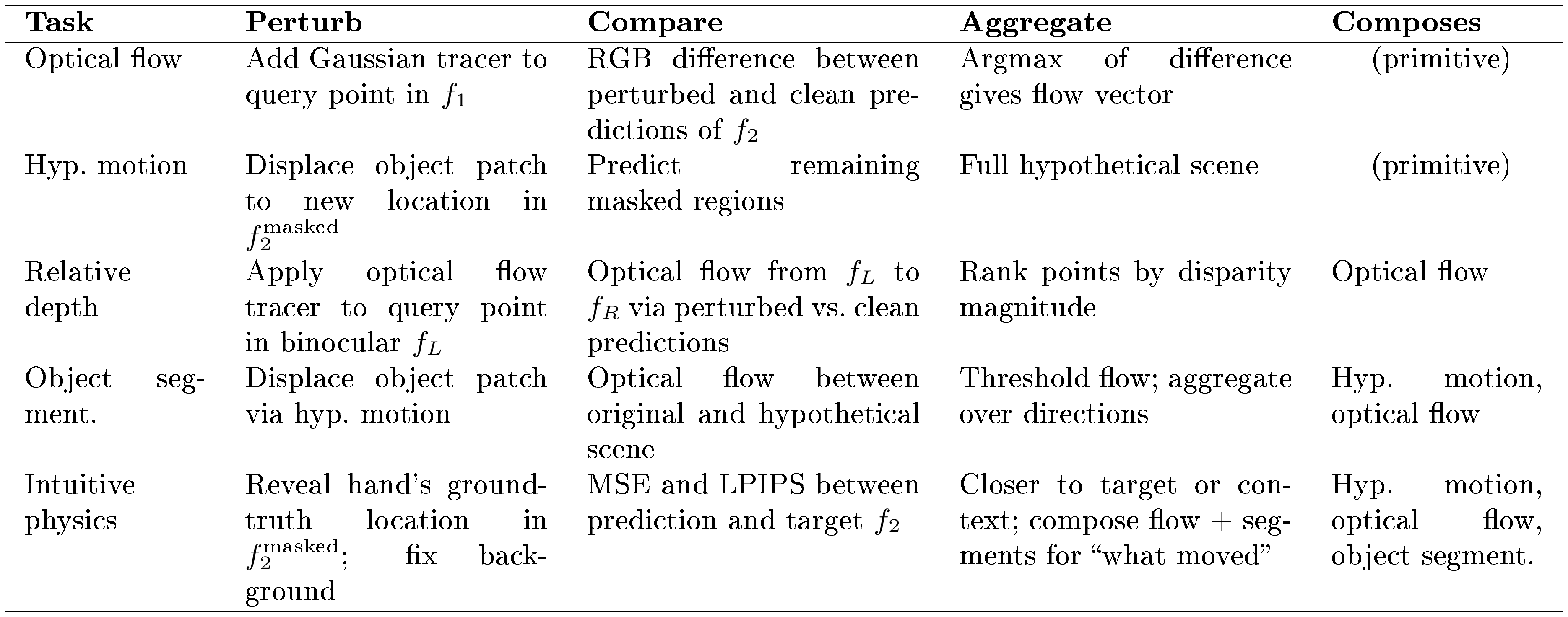
Optical flow (Figure 1 A). Latent cause: Between two frames $(f_1, f_2)$, a point at position $x_q$ in $f_1$ causes a corresponding point in $f_2$, due to the underlying causal structure of motion.

1. Perturb: Duplicate the initial frame $f_1$ and add a white-dot tracer to form $\tilde{f}_1$, using a Gaussian centered at the query location $x_q$ with amplitude 255 on each RGB channel and standard deviation $\sigma = 3.0$ pixels.
2. Compare: Run the model twice with the same masked second frame $f_2^{\text{masked}}$: once with the clean frame $(f_1, f_2^{\text{masked}}) \rightarrow \hat{f}_2$ and once with the perturbed frame $(\tilde{f}_1, f_2^{\text{masked}}) \rightarrow \tilde{f}_2^{\text{pred}}$. Compute the RGB difference $\Delta = \tilde{f}_2^{\text{pred}} - \hat{f}_2$.
3. Aggregate: Take the argmax of $|\Delta|$ to identify where the perturbation was carried to. The flow vector at $x_q$ is $\text{argmax}(|\Delta|) - x_q$.

Optical flow is the most primitive prompt and does not compose from other prompts; all subsequent prompts build on it. The masked patches in $f_2^{\text{masked}}$ are randomly selected and differ across evaluations, but are held fixed between the perturbed and unperturbed forward passes to ensure the flow signal can be localized.

Relative depth (Figure 1 D). Latent cause: The depth of a point is the latent cause governing its displacement under binocular separation; farther points exhibit smaller binocular disparity.

1. Perturb: Given a binocular image pair $(f_L, f_R)$ from stereo cameras, apply the optical flow tracer (as above) to a query point $x_q$ in $f_L$. Note that binocular image pairs are provided by the evaluation dataset; this is ecologically plausible, as humans possess binocular vision.
2. Compare: Compute the optical flow from $f_L$ to $f_R$ at $x_q$ by comparing the perturbed and unperturbed predictions, composing the optical flow prompt described above.
3. Aggregate: The magnitude of the resulting flow vector gives the binocular disparity at $x_q$, which is inversely related to depth. To compare relative depth of multiple points, compose multiple optical flow prompts and rank by disparity magnitude.

Hypothetical motion (Figure 2 A). Before describing the remaining prompts, we introduce a key primitive: hypothetical motion. ZWM simulates "what if this object moved?" by selecting one or more patches on an object and displacing them to a new location in $f_2^{\text{masked}}$, then predicting the remaining masked regions. The predictor propagates this local displacement to the rest of the object, producing a full hypothetical scene. While displacing a single patch often suffices, displacing multiple patches from the same object generally produces more coherent hypothetical scenes. This primitive is not evaluated directly but serves as a building block for object segmentation and intuitive physics below.

Object segmentation (Figure 2 A). Latent cause: Groups of pixels move together due to the latent cause of belonging to the same physical object—a learned form of "common fate" [88].

1. Perturb: Select a patch on a candidate object and displace it using the hypothetical motion primitive (above), producing a hypothetical scene $\tilde{f}$ in which the object has moved.
2. Compare: Compose the optical flow prompt to compute flow between the original image $f$ and the hypothetical prediction $\tilde{f}$. Pixels belonging to the perturbed object will exhibit coherent flow; other pixels will not.
3. Aggregate: Threshold the flow magnitude to produce a binary mask. Repeat over 8 displacement directions, with displacement magnitudes between 25 and 35 pixels, then aggregate the resulting masks to obtain the full object segment.

Intuitive physics (Figure 3 A). Latent cause: Physical interactions transmit forces between objects—e.g., pushing one object into another causes the second to move, exposing the underlying causal structure of contact dynamics.

1. Perturb: Reveal a $32 \times 32$-pixel green intervention patch in $f_2^{\text{masked}}$ at the hand's ground-truth location in the target frame, providing information about where the hand has moved. The hand location is annotated by human labelers, with care taken to ensure the patch does not reveal the object's position. This acts as a perturbation relative to the unperturbed case (where the hand's motion is masked and unknown), prompting the model to predict the physical consequences of the hand's action on the rest of the scene. Additional $32 \times 32$-pixel red background patches are revealed to fix illumination and camera pose, isolating the causal effect of the hand's motion on objects.
2. Compare: Compare the model's prediction (given the revealed hand motion) against the ground-truth target frame $f_2$, using both MSE and LPIPS perceptual similarity [27].
3. Aggregate: Determine whether the prediction is closer to the ground-truth target $f_2$ or the context frame $f_1$. Additionally, compose optical flow and object segmentation prompts on the predicted scene to evaluate what moved and how—e.g., whether force transferred to a second object.

1.3 Evaluation benchmarks

Optical flow: TAP-Vid benchmarks.

We evaluate optical flow on two benchmarks from the TAP-Vid suite:

• TAP-Vid-DAVIS [11]: Real-world videos with human-annotated ground-truth point correspondences, featuring challenging scenarios including fast motion, occlusions, and appearance changes.
• TAP-Vid-Kubric [12]: Synthetic, simulator-generated videos where ground-truth flows are known by construction, providing a complementary evaluation without annotation noise.

All evaluations are conducted at $256 \times 256$ resolution. For each algorithm, we report two standard TAP-Vid metrics [11]:

• Position accuracy (
  lt; \delta^x_{\text{avg}}$): For visible points, the fraction of predicted correspondences falling within a pixel-distance threshold of the ground-truth position, averaged over five thresholds (1, 2, 4, 8, and 16 pixels).
• Occlusion accuracy (OA): Binary classification accuracy for predicting whether each query point is occluded or out of frame on each time step.

Relative depth: UniQA-3D.

We evaluate relative depth estimation on UniQA-3D [16], which presents pairs of points and requires judging which is farther from the camera. The upright data originally contains 500 samples, but after filtering to ensure the query points fall unambiguously within the center crop of the image and that each image contains a stereo pair from the original KITTI dataset, the upright set is filtered to 103 examples and the flipped set to 61 examples.

Object segmentation: SpelkeBench.

We evaluate class-agnostic object segmentation on SpelkeBench [23], which defines objects as distinct, bounded physical entities. The benchmark draws images from two sources: 497 images from EntitySeg (real-world scenes) [89] and 51 images from OpenX (real-world robot interactions) [90], totaling 548 images. We measure performance using intersection-over-union (IoU) [25].

Intuitive physics benchmark.

We develop a novel short-timescale physical reasoning benchmark to evaluate models on intuitive physics (Figure 3 A). The benchmark features tabletop interactions between a hand and 1–2 objects, testing five categories of physical reasoning:

1. Object cohesion: When one part of an object is moved, the entire object moves together.
2. Support (top object moves): When a supporting surface is removed, the supported object falls.
3. Support (bottom object moves): When the bottom object in a stack is moved, the top object moves with it.
4. Force transfer: Pushing one object into another causes the second object to move.
5. Force separation: Moving one object does not affect a spatially separated object.

The benchmark contains 20 image pairs per category (100 image pairs total). Each image pair is evaluated under 8 different random mask configurations for the revealed patches in $f_2$, yielding $5 \times 20 \times 8 = 800$ total evaluations per model.

Each example consists of a context frame and a target frame. Accuracy is defined as the proportion of examples for which the model's prediction is closer to the ground-truth target than to the context frame, evaluated using both MSE and LPIPS [27].

Developmental trajectories.

To analyze developmental curves, we evaluate BabyZWM at various training checkpoints (0, 5k, 10k, 20k, 40k, 80k, 120k, 160k, 200k). Each ZWM model is trained for 200, 000 steps with a batch size of 512. As the videos are stored at 30 frames per second, this corresponds to $\sim$ 950 video hours, or roughly 95 days of waking experience assuming $\sim$ 10 awake hours per day for young children [28]. The $x$-axis represents training steps.

Neural predictivity.

We evaluate the alignment between model representations and biological neural responses using two complementary benchmarks:

• Natural Scenes Dataset (NSD) [51]: Human fMRI responses to natural images, capturing large-scale representational geometry.
• THINGS Ventral Stream Spiking Dataset (TVSD) [52]: Macaque single-neuron electrophysiology, revealing fine-grained neural tuning and timing.

For each model and brain region, we:

1. Extract features from every other layer of the model for each stimulus image.
2. Fit a cross-validated ridge regression from model features to neural responses.
3. Report noise-corrected Pearson correlations as the measure of neural predictivity.

For both NSD and TVSD, we use 10-fold cross-validation to split the data into training and test sets. Ridge regression regularization is performed using RidgeCV, which evaluates 21 regularization strengths ($\alpha$). Importantly, $\alpha$ is selected independently for each target (i.e., per voxel for fMRI, per neuron for electrophysiology), allowing the regularization to adapt to the noise characteristics of each recording site.

Noise ceilings are estimated differently for each dataset. For NSD, we use the reliability estimation method described by Allen et al. [51]. For TVSD, noise ceilings are computed via split-half correlations. For NSD, neural predictivity is evaluated for V1, V2, V4, and the anterior ventral visual regions. For TVSD, we evaluate using V1, V4, and inferior temporal (IT) cortex.

1.4 Baselines

We compare ZWM against both representation-based models and task-specific systems.

Representation-based models.

Unlike ZWM, representation-based models are not natively zero-shot and typically require labeled supervision (fine-tuning or linear probes) for each downstream task. To enable fair comparison, we design simple zero-shot probes for these models:

• ResNet50 (ImageNet-supervised): A standard ResNet50 [91] pretrained on ImageNet-1K with category-label supervision.
• Baby DINOv3: DINOv3 [9] (ViT-Large) learns single-image representations by training the model to produce consistent features across different augmented views of the same image. We train DINOv3 on BabyView (868 hours).
• Baby V-JEPA2: V-JEPA2 is a self-supervised video model that learns by predicting masked regions of a video in feature space rather than in raw pixels. We train a 300-million parameter V-JEPA2 model on BabyView (868 hours) using the official implementation and default hyperparameters. We verified successful training via frozen linear probes on held-out subsets, yielding 54.2% top-1 accuracy on Kinetics-400 (400-way classification) and 53.45% on ImageNet-1K (1000-way classification) [92].

Zero-shot probe designs for representation-based baselines.

Since ResNet50, DINOv3 and V-JEPA2 are representation-based models that do not natively support zero-shot visual-cognitive extraction, we design simple probe procedures to enable fair comparison.

Optical flow. For ResNet50, DINOv3 and V-JEPA2, we pass both frames through the model and extract patch-level feature representations. To estimate the flow at a query point in the first frame, we compute the cosine similarity between the query point's patch feature in the first frame and all patch features in the second frame. The target location is taken as the patch in the second frame with the highest cosine similarity, and the flow vector is the displacement between the query and target positions.

Relative depth. We apply the same cosine-similarity correspondence matching procedure described above for optical flow to binocular image pairs, and infer relative depth from the magnitude of the resulting disparity (optical flow) vector, following the same logic as the ZWM depth prompt.

Object segmentation. We compute pairwise cosine similarity between all patch features within each image. Object segments are obtained by thresholding the cosine similarity to a seed patch, grouping patches with high feature similarity as belonging to the same object.

Intuitive physics. ResNet50 and DINOv3 are single-image models and cannot be meaningfully evaluated on our temporal intuitive physics benchmark, so they are excluded from this comparison. For V-JEPA2, we provide the same revealed patches (hand location and background grounding patches) as input and use V-JEPA2 to predict representations for the masked patches. We then compute the cosine similarity between the predicted representations and the representations of the same regions extracted from (i) the initial context frame $f_1$ and (ii) the ground-truth target frame $f_2$. If the predicted representations are more similar to $f_2$ than to $f_1$, the model is scored as correct.

Task-specific baselines.

For each visual-cognitive task, we compare against state-of-the-art task-specific models:

• Optical flow: CoTracker3 [13], DPFlow [14], and SeaRAFT [15]. All are supervised models trained with ground-truth flow annotations.
• Relative depth: MiDaS-CNN (supervised monocular) [20], MonoDepth2 (self-supervised monocular) [21], and FoundationStereo (supervised binocular) [22]. We also compare against large vision-language models: Gemini-1.5 [17], GPT-4-Turbo [18], and GPT-4o [19].
• Object segmentation: Mask2Former [24] (trained on COCO [25]) and SAM2 [26] (trained with large-scale human annotations).
• Intuitive physics: No established baselines exist for our novel benchmark; we compare against V-JEPA2 and Baby V-JEPA2.

Supplementary Text

Section Summary: The supplementary text examines how the BabyZWM AI model processes intuitive physics by analyzing attention patterns in its transformer layers, revealing that deeper layers focus more on the hand—the agent causing object motion—compared to background or random areas, which suggests the model learns causal relationships in physical events. It also presents evidence that the model's internal representations align hierarchically with brain activity, as early layers correspond to lower visual brain regions and deeper layers to higher ones, based on human fMRI data and monkey neuron recordings. This alignment is comparable to models trained on larger datasets, supporting the model's realistic simulation of visual processing.

Attention head analysis for intuitive physics

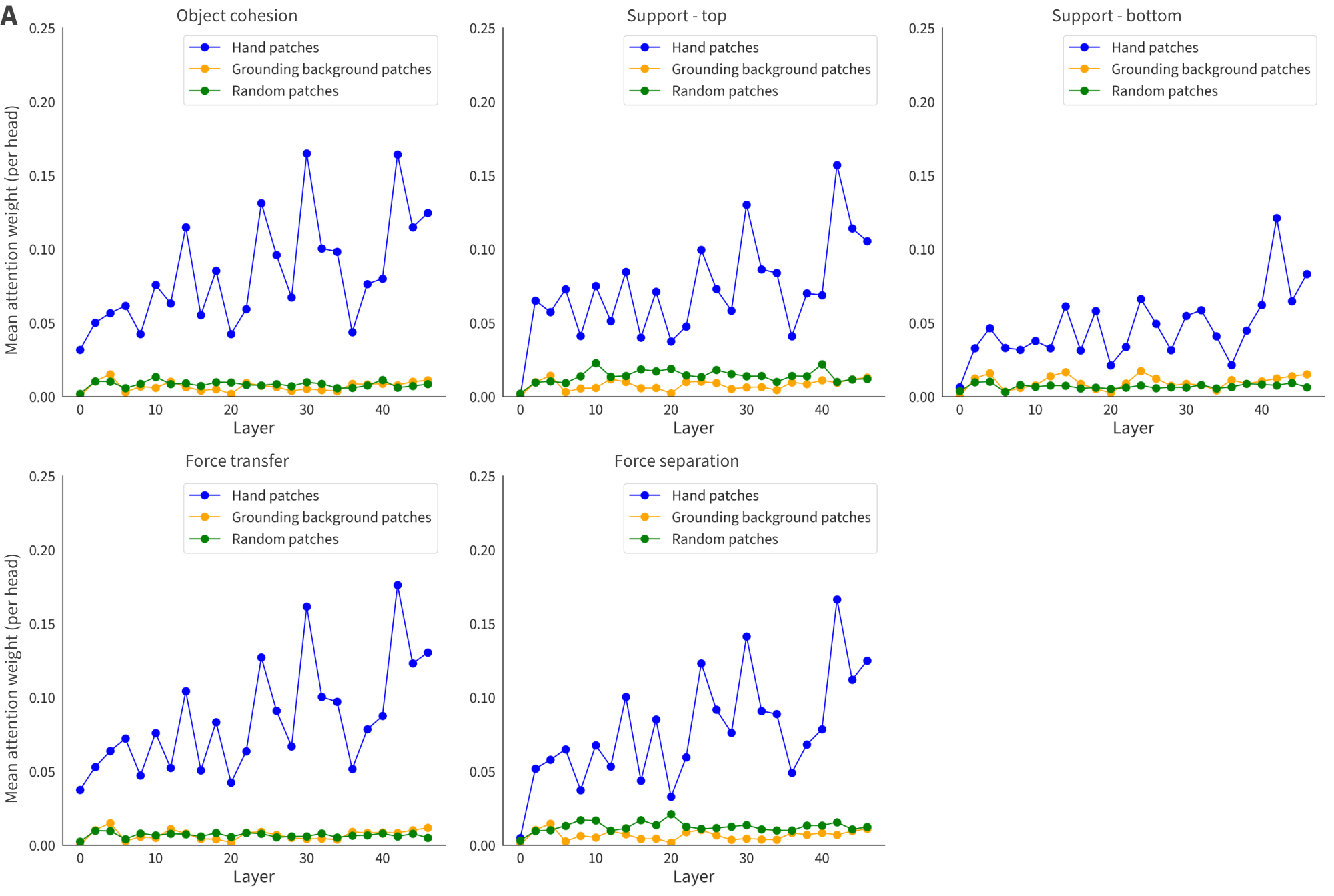
To understand how BabyZWM implements intuitive physical reasoning internally, we analyze the attention patterns of individual transformer heads during the intuitive physics evaluation.

Methodology.

For each intuitive physics example, we extract the full attention weight tensor across all layers and heads during the factual prediction forward pass. The model receives two frames as input: the context frame $f_1$ (1024 tokens) and the partially unmasked target frame $f_2$ (1024 tokens), yielding 2048 total tokens. We select a query patch located on the moved object in $f_2$ (identified from human annotations of the object's position in the target frame) and examine which tokens this query patch attends to across all layers.

We partition the key tokens into three groups:

• Hand patches: The 16 patches (forming a $4 \times 4$ patch region, i.e., $32 \times 32$ pixels) centered on the hand's revealed location in $f_2$ —the causal agent responsible for the object's motion.
• Background grounding patches: The patches revealed at fixed background locations (top and bottom image borders) that anchor camera pose and illumination, providing non-causal contextual information.
• Random patches: An equal number of patches sampled randomly from $f_2$, excluding hand and background patches, serving as a baseline.

Quantitative analysis.

For each layer, we compute the average attention weight (averaged across all heads) from the query patch to each of the three patch groups. To ensure comparability across groups of different sizes, we normalize the background attention by the ratio of background patches to hand patches. We average these layer-wise attention profiles across all examples within each intuitive physics category (e.g., object cohesion, support, force transfer) and across 8 random seeds.

Results.

The layer-wise attention profiles reveal that in deeper transformer layers, attention from the moved object's query patch tends to be disproportionately allocated to the hand patches relative to both background grounding patches and random patches. This pattern is broadly consistent across intuitive physics categories, suggesting that the model may have learned to preferentially attend to the hand—the causal agent of object motion—when predicting physical outcomes. While these attention patterns are consistent with a "causal attention" interpretation, we note that attention weights are an indirect measure of the model's internal computations, and further mechanistic work would be needed to confirm whether these heads play a causal role in the model's physical predictions. Nonetheless, the emergence of hand-directed attention in deeper layers is suggestive of a hierarchical computation in which later layers begin to integrate information about agent–object relationships relevant to physical prediction. Layer-wise attention profiles for each intuitive physics category are shown in Figure 6.

Neural predictivity results

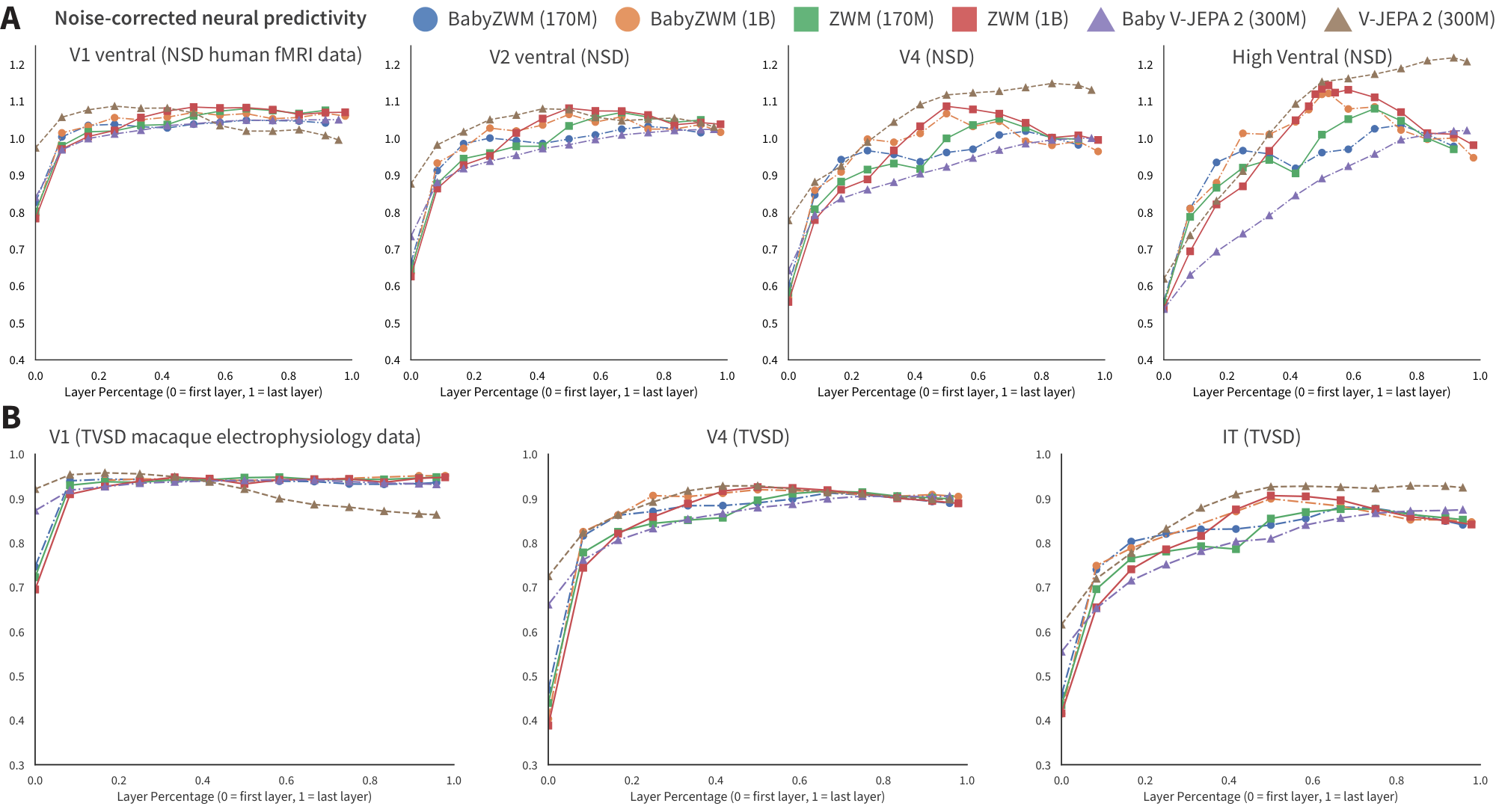
In the main text, we reported that BabyZWM's internal representations align with hierarchical visual cortex organization using the Natural Scenes Dataset (NSD) [51]. Here we present expanded neural predictivity results across both NSD (human fMRI) and the THINGS Ventral Stream Spiking Dataset (TVSD; macaque single-neuron electrophysiology) [52], providing converging evidence across species and measurement modalities.

Across both benchmarks, BabyZWM exhibits hierarchically organized layer-area correspondence: earlier model layers best predict earlier cortical regions, while deeper layers align with higher visual areas. In NSD, this pattern is evident across all evaluated ROIs; TVSD corroborates these findings at single-neuron resolution, confirming that the representational hierarchy is not an artifact of the fMRI measurement scale. BabyZWM achieves predictivity comparable to ZWM variants trained on substantially larger and more diverse datasets, whereas Baby V-JEPA2 shows lower neural alignment than its larger-data counterpart. Full layer-by-region predictivity profiles for both benchmarks are shown in Figure 7.

References

Section Summary: This references section compiles a bibliography of academic papers, books, and datasets central to research in artificial intelligence and cognitive science. It features recent studies on machine vision techniques, such as transformers for image recognition, self-supervised video models, optical flow estimation, and depth perception, alongside foundational works on causality and counterfactual reasoning in both AI and human cognition. The list also includes resources on egocentric videos of infants, human action datasets, segmentation tools, and child development topics like sleep duration and object tracking in young children.

[1] Bear et al. (2023). Unifying (Machine) Vision via Counterfactual World Modeling. arXiv:2306.01828 [cs]. http://arxiv.org/abs/2306.01828.

[2] He et al. (2021). Masked Autoencoders Are Scalable Vision Learners. arXiv:2111.06377 [cs]. http://arxiv.org/abs/2111.06377.

[3] Pearl, Judea (2009). Causality: Models, Reasoning and Inference. Cambridge University Press.

[4] Gerstenberg, Tobias (2024). Counterfactual simulation in causal cognition. doi:10.31234/osf.io/72scr. https://osf.io/72scr.

[5] Dosovitskiy et al. (2021). An Image is Worth 16x16 Words: Transformers for Image Recognition at Scale. arXiv:2010.11929 [cs]. doi:10.48550/arXiv.2010.11929. http://arxiv.org/abs/2010.11929.

[6] Long et al. (2024). The BabyView dataset: High-resolution egocentric videos of infants' and young children's everyday experiences. arXiv:2406.10447 [cs]. http://arxiv.org/abs/2406.10447.

[7] Kay et al. (2017). The Kinetics Human Action Video Dataset. arXiv:1705.06950 [cs]. doi:10.48550/arXiv.1705.06950. http://arxiv.org/abs/1705.06950.

[8] Kotar et al. (2025). World Modeling with Probabilistic Structure Integration. arXiv:2509.09737 [cs]. doi:10.48550/arXiv.2509.09737. http://arxiv.org/abs/2509.09737.

[9] Siméoni et al. (2025). DINOv3. arXiv:2508.10104 [cs]. doi:10.48550/arXiv.2508.10104. http://arxiv.org/abs/2508.10104.

[10] Assran et al. (2025). V-JEPA 2: Self-Supervised Video Models Enable Understanding, Prediction and Planning. arXiv:2506.09985 [cs]. doi:10.48550/arXiv.2506.09985. http://arxiv.org/abs/2506.09985.

[11] Doersch et al. (2023). TAP-Vid: A Benchmark for Tracking Any Point in a Video. arXiv:2211.03726 [cs]. doi:10.48550/arXiv.2211.03726. http://arxiv.org/abs/2211.03726.

[12] Greff et al. (2022). Kubric: A scalable dataset generator. arXiv:2203.03570 [cs]. doi:10.48550/arXiv.2203.03570. http://arxiv.org/abs/2203.03570.

[13] Karaev et al. (2024). CoTracker: It is Better to Track Together. arXiv:2307.07635 [cs]. doi:10.48550/arXiv.2307.07635. http://arxiv.org/abs/2307.07635.

[14] Morimitsu et al. (2025). DPFlow: Adaptive Optical Flow Estimation with a Dual-Pyramid Framework. arXiv:2503.14880 [cs]. doi:10.48550/arXiv.2503.14880. http://arxiv.org/abs/2503.14880.

[15] Wang et al. (2024). SEA-RAFT: Simple, Efficient, Accurate RAFT for Optical Flow. arXiv:2405.14793 [cs]. doi:10.48550/arXiv.2405.14793. http://arxiv.org/abs/2405.14793.

[16] Zuo et al. (2024). Towards Foundation Models for 3D Vision: How Close Are We?. arXiv:2410.10799 [cs]. http://arxiv.org/abs/2410.10799.

[17] Gemini et al. (2024). Gemini 1.5: Unlocking multimodal understanding across millions of tokens of context. arXiv:2403.05530 [cs]. doi:10.48550/arXiv.2403.05530. http://arxiv.org/abs/2403.05530.

[18] OpenAI et al. (2024). GPT-4 Technical Report. arXiv:2303.08774 [cs]. doi:10.48550/arXiv.2303.08774. http://arxiv.org/abs/2303.08774.

[19] OpenAI et al. (2024). GPT-4o System Card. arXiv:2410.21276 [cs]. doi:10.48550/arXiv.2410.21276. http://arxiv.org/abs/2410.21276.

[20] Ranftl et al. (2020). Towards Robust Monocular Depth Estimation: Mixing Datasets for Zero-shot Cross-dataset Transfer. arXiv:1907.01341 [cs]. doi:10.48550/arXiv.1907.01341. http://arxiv.org/abs/1907.01341.

[21] Godard et al. (2019). Digging Into Self-Supervised Monocular Depth Estimation. arXiv:1806.01260 [cs]. doi:10.48550/arXiv.1806.01260. http://arxiv.org/abs/1806.01260.

[22] Wen et al. (2025). FoundationStereo: Zero-Shot Stereo Matching. arXiv:2501.09898 [cs]. doi:10.48550/arXiv.2501.09898. http://arxiv.org/abs/2501.09898.

[23] Venkatesh et al. (2025). Discovering and using Spelke segments. arXiv:2507.16038 [cs]. doi:10.48550/arXiv.2507.16038. http://arxiv.org/abs/2507.16038.

[24] Cheng et al. (2022). Masked-attention Mask Transformer for Universal Image Segmentation. arXiv:2112.01527 [cs]. doi:10.48550/arXiv.2112.01527. http://arxiv.org/abs/2112.01527.

[25] Lin et al. (2015). Microsoft COCO: Common Objects in Context. arXiv:1405.0312 [cs]. doi:10.48550/arXiv.1405.0312. http://arxiv.org/abs/1405.0312.

[26] Ravi et al. (2024). SAM 2: Segment Anything in Images and Videos. arXiv:2408.00714 [cs]. doi:10.48550/arXiv.2408.00714. http://arxiv.org/abs/2408.00714.

[27] Zhang et al. (2018). The Unreasonable Effectiveness of Deep Features as a Perceptual Metric. arXiv:1801.03924 [cs]. doi:10.48550/arXiv.1801.03924. http://arxiv.org/abs/1801.03924.

[28] Iglowstein et al. (2003). Sleep Duration From Infancy to Adolescence: Reference Values and Generational Trends. Pediatrics. 111(2). pp. 302–307. doi:10.1542/peds.111.2.302. https://publications.aap.org/pediatrics/article/111/2/302/66745/Sleep-Duration-From-Infancy-to-Adolescence.

[29] Trick et al. (2005). Multiple-object tracking in children: The “Catch the Spies” task. Cognitive Development. 20(3). pp. 373–387. doi:10.1016/j.cogdev.2005.05.009. https://linkinghub.elsevier.com/retrieve/pii/S0885201405000249.

[30] Blankenship et al. (2020). Development of multiple object tracking via multifocal attention.. Developmental Psychology. 56(9). pp. 1684–1695. doi:10.1037/dev0001064. https://doi.apa.org/doi/10.1037/dev0001064.

[31] Held et al. (1980). Stereoacuity of human infants.. Proceedings of the National Academy of Sciences. 77(9). pp. 5572–5574. doi:10.1073/pnas.77.9.5572. https://pnas.org/doi/full/10.1073/pnas.77.9.5572.

[32] Fox et al. (1980). Stereopsis in Human Infants. Science. 207(4428). pp. 323–324. doi:10.1126/science.7350666. https://www.science.org/doi/10.1126/science.7350666.

[33] Birch et al. (1982). Stereoacuity development for crossed and uncrossed disparities in human infants. Vision Research. 22(5). pp. 507–513. doi:10.1016/0042-6989(82)90108-0. https://linkinghub.elsevier.com/retrieve/pii/0042698982901080.

[34] Norcia et al. (2025). Late Development of Sensory Thresholds for Horizontal Relative Disparity in Human Visual Cortex in the Face of Precocial Development of Thresholds for Absolute Disparity. The Journal of Neuroscience. 45(7). pp. e0216242024. doi:10.1523/JNEUROSCI.0216-24.2024. https://www.jneurosci.org/lookup/doi/10.1523/JNEUROSCI.0216-24.2024.

[35] Johnson, Scott P. (2010). How Infants Learn About the Visual World. Cognitive Science. 34(7). pp. 1158–1184. doi:10.1111/j.1551-6709.2010.01127.x. https://onlinelibrary.wiley.com/doi/10.1111/j.1551-6709.2010.01127.x.

[36] Baillargeon et al. (2012). Object Individuation and Physical Reasoning in Infancy: An Integrative Account. Language Learning and Development. 8(1). pp. 4–46. doi:10.1080/15475441.2012.630610. http://www.tandfonline.com/doi/abs/10.1080/15475441.2012.630610.

[37] Baillargeon et al. (1992). The development of young infants' intuitions about support. Early Development and Parenting. 1(2). pp. 69–78. doi:10.1002/edp.2430010203. https://onlinelibrary.wiley.com/doi/10.1002/edp.2430010203.

[38] Hespos, Susan J and Baillargeon, Renée (2001). Reasoning about containment events in very young infants. Cognition. 78(3). pp. 207–245. doi:10.1016/S0010-0277(00)00118-9. https://linkinghub.elsevier.com/retrieve/pii/S0010027700001189.

[39] Schrimpf et al. (2018). Brain-Score: Which Artificial Neural Network for Object Recognition is most Brain-Like?. doi:10.1101/407007. http://biorxiv.org/lookup/doi/10.1101/407007.

[40] Felleman, D. J. and Van Essen, D. C. (1991). Distributed Hierarchical Processing in the Primate Cerebral Cortex. Cerebral Cortex. 1(1). pp. 1–47. doi:10.1093/cercor/1.1.1. https://academic.oup.com/cercor/article-lookup/doi/10.1093/cercor/1.1.1.

[41] DiCarlo et al. (2012). How Does the Brain Solve Visual Object Recognition?. Neuron. 73(3). pp. 415–434. doi:10.1016/j.neuron.2012.01.010. https://linkinghub.elsevier.com/retrieve/pii/S089662731200092X.

[42] Grill-Spector, Kalanit and Weiner, Kevin S. (2014). The functional architecture of the ventral temporal cortex and its role in categorization. Nature Reviews Neuroscience. 15(8). pp. 536–548. doi:10.1038/nrn3747. https://www.nature.com/articles/nrn3747.

[43] Gogtay et al. (2004). Dynamic mapping of human cortical development during childhood through early adulthood. Proceedings of the National Academy of Sciences. 101(21). pp. 8174–8179. doi:10.1073/pnas.0402680101. https://pnas.org/doi/full/10.1073/pnas.0402680101.

[44] Golarai et al. (2007). Differential development of high-level visual cortex correlates with category-specific recognition memory. Nature Neuroscience. 10(4). pp. 512–522. doi:10.1038/nn1865. https://www.nature.com/articles/nn1865.

[45] Grill-Spector et al. (2008). Developmental neuroimaging of the human ventral visual cortex. Trends in Cognitive Sciences. 12(4). pp. 152–162. doi:10.1016/j.tics.2008.01.009. https://linkinghub.elsevier.com/retrieve/pii/S1364661308000570.

[46] Braddick, Oliver and Atkinson, Janette (2011). Development of human visual function. Vision Research. 51(13). pp. 1588–1609. doi:10.1016/j.visres.2011.02.018. https://linkinghub.elsevier.com/retrieve/pii/S004269891100068X.

[47] Kiorpes, Lynne (2015). Visual development in primates: Neural mechanisms and critical periods. Developmental Neurobiology. 75(10). pp. 1080–1090. doi:10.1002/dneu.22276. https://onlinelibrary.wiley.com/doi/10.1002/dneu.22276.

[48] Yamins et al. (2014). Performance-optimized hierarchical models predict neural responses in higher visual cortex. Proceedings of the National Academy of Sciences. 111(23). pp. 8619–8624. doi:10.1073/pnas.1403112111. https://pnas.org/doi/full/10.1073/pnas.1403112111.

[49] Guclu, U. and Van Gerven, M. A. J. (2015). Deep Neural Networks Reveal a Gradient in the Complexity of Neural Representations across the Ventral Stream. Journal of Neuroscience. 35(27). pp. 10005–10014. doi:10.1523/JNEUROSCI.5023-14.2015. https://www.jneurosci.org/lookup/doi/10.1523/JNEUROSCI.5023-14.2015.

[50] Yamins, Daniel L K and DiCarlo, James J (2016). Using goal-driven deep learning models to understand sensory cortex. Nature Neuroscience. 19(3). pp. 356–365. doi:10.1038/nn.4244. https://www.nature.com/articles/nn.4244.

[51] Allen et al. (2022). A massive 7T fMRI dataset to bridge cognitive neuroscience and artificial intelligence. Nature Neuroscience. 25(1). pp. 116–126. doi:10.1038/s41593-021-00962-x. https://www.nature.com/articles/s41593-021-00962-x.

[52] Papale et al. (2025). An extensive dataset of spiking activity to reveal the syntax of the ventral stream. Neuron. 113(4). pp. 539–553.e5. doi:10.1016/j.neuron.2024.12.003. https://linkinghub.elsevier.com/retrieve/pii/S089662732400881X.

[53] Goodale, Melvyn A. and Milner, A.David (1992). Separate visual pathways for perception and action. Trends in Neurosciences. 15(1). pp. 20–25. doi:10.1016/0166-2236(92)90344-8. https://linkinghub.elsevier.com/retrieve/pii/0166223692903448.

[54] Kaplan, David Michael and Craver, Carl F. (2011). The Explanatory Force of Dynamical and Mathematical Models in Neuroscience: A Mechanistic Perspective. Philosophy of Science. 78(4). pp. 601–627. doi:10.1086/661755. https://www.cambridge.org/core/product/identifier/S0031824800016093/type/journal_article.

[55] Cao, Rosa and Yamins, Daniel (2021). Explanatory models in neuroscience: Part 1 – taking mechanistic abstraction seriously. arXiv:2104.01490 [cs, q-bio]. http://arxiv.org/abs/2104.01490.

[56] Frank, Michael C. (2025). Cognitive modeling using artificial intelligence. doi:10.31234/osf.io/wv7mg_v1. https://osf.io/wv7mg_v1.

[57] Orhan et al. (2020). Self-supervised learning through the eyes of a child. arXiv:2007.16189 [cs]. http://arxiv.org/abs/2007.16189.

[58] Zhuang et al. (2021). Unsupervised neural network models of the ventral visual stream. Proceedings of the National Academy of Sciences. 118(3). pp. e2014196118. doi:10.1073/pnas.2014196118.

[59] Sheybani et al. (2023). Curriculum Learning with Infant Egocentric Videos.

[60] Orhan et al. (2024). Self-supervised learning of video representations from a child's perspective. arXiv:2402.00300 [cs, q-bio]. http://arxiv.org/abs/2402.00300.

[61] Wu et al. (2018). Unsupervised Feature Learning via Non-Parametric Instance-level Discrimination. arXiv:1805.01978 [cs]. doi:10.48550/arXiv.1805.01978. http://arxiv.org/abs/1805.01978.

[62] Zhuang et al. (2019). Local Aggregation for Unsupervised Learning of Visual Embeddings. In 2019 IEEE/CVF International Conference on Computer Vision (ICCV). pp. 6001–6011. doi:10.1109/ICCV.2019.00610. https://ieeexplore.ieee.org/document/9011034/.

[63] Chen et al. (2020). A Simple Framework for Contrastive Learning of Visual Representations. arXiv:2002.05709 [cs, stat]. http://arxiv.org/abs/2002.05709.

[64] Grill et al. (2020). Bootstrap your own latent: A new approach to self-supervised Learning. arXiv:2006.07733 [cs]. doi:10.48550/arXiv.2006.07733. http://arxiv.org/abs/2006.07733.

[65] Tong et al. (2022). VideoMAE: Masked Autoencoders are Data-Efficient Learners for Self-Supervised Video Pre-Training. arXiv:2203.12602 [cs]. doi:10.48550/arXiv.2203.12602. http://arxiv.org/abs/2203.12602.

[66] Caron et al. (2021). Emerging Properties in Self-Supervised Vision Transformers. arXiv:2104.14294 [cs]. doi:10.48550/arXiv.2104.14294. http://arxiv.org/abs/2104.14294.

[67] Bardes et al. (2024). Revisiting Feature Prediction for Learning Visual Representations from Video. arXiv:2404.08471 [cs]. http://arxiv.org/abs/2404.08471.

[68] Sutton, Richard (2019). The Bitter Lesson. Essay.

[69] Spelke et al. (1992). Origins of knowledge.. Psychological Review. 99(4). pp. 605–632. doi:10.1037/0033-295X.99.4.605. https://doi.apa.org/doi/10.1037/0033-295X.99.4.605.

[70] Spelke, Elizabeth S. (2000). Core knowledge.. American Psychologist. 55(11). pp. 1233–1243. doi:10.1037/0003-066X.55.11.1233. https://doi.apa.org/doi/10.1037/0003-066X.55.11.1233.

[71] Carey, Susan (2009). The origin of concepts. Oxford University Press.

[72] Spelke, Elizabeth S. (2022). What Babies Know: Core Knowledge and Composition Volume 1. Oxford University PressNew York. doi:10.1093/oso/9780190618247.001.0001. https://academic.oup.com/book/43912.

[73] Chomsky, Noam (1980). Rules and representations. Behavioral and Brain Sciences. 3(1). pp. 1–15. doi:10.1017/S0140525X00001515. https://www.cambridge.org/core/product/identifier/S0140525X00001515/type/journal_article.

[74] Lasnik, Howard and Lidz, Jeffrey L. (2016). The Argument from the Poverty of the Stimulus. doi:10.1093/oxfordhb/9780199573776.013.10. https://academic.oup.com/edited-volume/27996/chapter/211719982.

[75] Sutton, Richard S. (1990). Integrated Architectures for Learning, Planning, and Reacting Based on Approximating Dynamic Programming. doi:10.1016/B978-1-55860-141-3.50030-4. https://linkinghub.elsevier.com/retrieve/pii/B9781558601413500304.

[76] Marc Peter Deisenroth and Carl Edward Rasmussen (2011). PILCO: A Model-Based and Data-Efficient Approach to Policy Search. In International Conference on Machine Learning. https://api.semanticscholar.org/CorpusID:14273320.

[77] García et al. (1989). Model predictive control: Theory and practice—A survey. Automatica. 25(3). pp. 335–348. doi:https://doi.org/10.1016/0005-1098(89)90002-2. https://www.sciencedirect.com/science/article/pii/0005109889900022.

[78] Ha, David and Schmidhuber, Jürgen (2018). World Models. doi:10.5281/zenodo.1207631. http://arxiv.org/abs/1803.10122.

[79] Danijar Hafner et al. (2019). Dream to Control: Learning Behaviors by Latent Imagination. ArXiv. abs/1912.01603. https://api.semanticscholar.org/CorpusID:208547755.

[80] Danijar Hafner et al. (2018). Learning Latent Dynamics for Planning from Pixels. ArXiv. abs/1811.04551. https://api.semanticscholar.org/CorpusID:53280207.

[81] Danijar Hafner et al. (2022). Deep Hierarchical Planning from Pixels. ArXiv. abs/2206.04114. https://api.semanticscholar.org/CorpusID:249538516.

[82] Lukasz Kaiser et al. (2019). Model-Based Reinforcement Learning for Atari. ArXiv. abs/1903.00374. https://api.semanticscholar.org/CorpusID:67856232.

[83] Julian Schrittwieser et al. (2019). Mastering Atari, Go, chess and shogi by planning with a learned model. Nature. 588. pp. 604 - 609. https://api.semanticscholar.org/CorpusID:208158225.

[84] Philipp Wu et al. (2022). DayDreamer: World Models for Physical Robot Learning. In Conference on Robot Learning. https://api.semanticscholar.org/CorpusID:250088882.

[85] Kotar et al. (2023). ENTL: Embodied Navigation Trajectory Learner. In Proceedings of the IEEE/CVF International Conference on Computer Vision (ICCV). pp. 10863-10872.

[86] Lee et al. (2025). 3D Scene Understanding Through Local Random Access Sequence Modeling. arXiv:2504.03875 [cs]. doi:10.48550/arXiv.2504.03875. http://arxiv.org/abs/2504.03875.

[87] Kim et al. (2025). Taming generative video models for zero-shot optical flow extraction. arXiv:2507.09082 [cs]. doi:10.48550/arXiv.2507.09082. http://arxiv.org/abs/2507.09082.

[88] Kellman, Philip J. and Spelke, Elizabeth S. (1983). Perception of partly occluded objects in infancy. Cognitive Psychology. 15(4). pp. 483–524. doi:10.1016/0010-0285(83)90017-8. https://linkinghub.elsevier.com/retrieve/pii/0010028583900178.

[89] Qi et al. (2023). High-Quality Entity Segmentation. arXiv:2211.05776 [cs]. doi:10.48550/arXiv.2211.05776. http://arxiv.org/abs/2211.05776.

[90] Collaboration et al. (2025). Open X-Embodiment: Robotic Learning Datasets and RT-X Models. arXiv:2310.08864 [cs]. doi:10.48550/arXiv.2310.08864. http://arxiv.org/abs/2310.08864.

[91] He et al. (2015). Deep Residual Learning for Image Recognition. arXiv:1512.03385 [cs]. doi:10.48550/arXiv.1512.03385. http://arxiv.org/abs/1512.03385.

[92] Deng et al. (2009). ImageNet: A large-scale hierarchical image database. In 2009 IEEE Conference on Computer Vision and Pattern Recognition. pp. 248–255. doi:10.1109/CVPR.2009.5206848. https://ieeexplore.ieee.org/document/5206848/.