Who Said Neural Networks Aren't Linear?

Nimrod Berman$^{*}$
Ben-Gurion University
[email protected]

Assaf Hallak$^{*}$
NVIDIA
[email protected]

Assaf Shocher$^{*\dagger}$
Technion
[email protected]

$^{*}$Equal contribution.
$^{\dagger}$A.S. is a Chaya Fellow, supported by the Chaya Career Advancement Chair.
Code available at https://github.com/assafshocher/Linearizer

Keywords: Deep Learning, Linearity, Invertible Networks, Diffusion

Abstract

Neural networks are famously nonlinear. However, linearity is defined relative to a pair of vector spaces, $f:\mathcal{X}\to\mathcal{Y}$. Leveraging the algebraic concept of transport of structure, we propose a method to explicitly identify non-standard vector spaces where a neural network acts as a linear operator. When sandwiching a linear operator $A$ between two invertible neural networks, $f(x)=g_y^{-1}(A g_x(x))$, the corresponding vector spaces $\mathcal{X}$ and $\mathcal{Y}$ are induced by newly defined addition and scaling actions derived from $g_x$ and $g_y$. We term this kind of architecture a Linearizer. This framework makes the entire arsenal of linear algebra, including SVD, pseudo-inverse, orthogonal projection and more, applicable to nonlinear mappings. Furthermore, we show that the composition of two Linearizers that share a neural network is also a Linearizer. We leverage this property and demonstrate that training diffusion models using our architecture makes the hundreds of sampling steps collapse into a single step. We further utilize our framework to enforce idempotency (i.e. $f(f(x))=f(x)$) on networks leading to a globally projective generative model and to demonstrate modular style transfer.

Executive Summary: Neural networks, the backbone of modern artificial intelligence, excel at complex tasks like image generation and pattern recognition because they are nonlinear. However, this nonlinearity makes them hard to analyze, manipulate, or optimize using the powerful tools of linear algebra—such as decomposition, inversion, or efficient iteration—that work seamlessly on simpler systems. As AI models grow larger and are deployed in real-time applications like content creation or simulation, the need for more tractable nonlinear models has become urgent. This work addresses that gap by introducing a way to redefine the underlying mathematical spaces so that neural networks behave as linear operators, unlocking these tools without losing the networks' expressive power.

The document sets out to demonstrate a new architecture called the Linearizer, which transforms a nonlinear neural network into a linear one relative to custom vector spaces. In plain terms, it evaluates whether this setup can fit data as well as standard networks while enabling applications that are otherwise difficult or impossible.

The authors developed the Linearizer by placing a simple linear matrix between two invertible neural networks, which act like coordinate transformations. These components are trained together end-to-end on standard datasets, using invertible architectures like coupling layers to ensure reversibility. The approach draws on established data sources such as MNIST for digits, CelebA for faces, and dSprites for shape variations, over training periods typical for such models (not specified in detail but feasible on consumer hardware). Key assumptions include the ability of invertible networks to approximate smooth transformations and the sufficiency of a low-rank linear core for efficiency. No advanced math is needed here; the focus is on practical implementation, with code provided for replication.

The core findings center on three main applications. First, in generative modeling like diffusion models—which normally require hundreds of iterative steps to create images from noise—the Linearizer collapses this process into a single step. Tests on MNIST and CelebA showed that one-step outputs match multi-step results with errors below 0.0003, and image quality scores (FID) improved by about 8 points when simulating finer steps mathematically rather than iteratively. Second, for style transfer in images, the framework allows modular mixing of styles via simple matrix operations; interpolating between styles like "mosaic" and "candy" produced smooth, coherent blends without retraining. Third, it enforces idempotency—meaning applying the model twice yields the same result as once—architecturally, creating stable generative projectors that work globally, not just on training data. Additional tests confirmed competitiveness: 87.6% accuracy on face attribute classification (better than a ResNet baseline), preserved disentanglement in variational autoencoders, and near-matching performance in weather forecasting against specialized models.

These results mean that nonlinear neural networks can now borrow linear algebra's efficiencies, reducing computation by orders of magnitude in tasks like image generation (from hundreds to one step) and enabling precise control, such as inverting mappings for editing or projecting data onto manifolds for robustness. This differs from prior work, like approximations in Koopman theory or distillation methods, by guaranteeing exact linearity without extra optimization tricks, which lowers risks of instability or errors in deployment. For businesses, it could cut inference costs and energy use in AI tools, while improving safety through built-in properties like idempotency that prevent erratic outputs.

Next steps should prioritize scaling the Linearizer to larger datasets and higher resolutions, such as full HD images or video, to compete with top generative models. Pilot integrations into existing pipelines—for instance, accelerating diffusion-based tools in creative software—would validate real-world gains. Options include focusing on generation for speed or idempotency for reliable editing; the former trades some quality for efficiency, while the latter prioritizes stability but may need more training data. Further analysis on diverse domains like time-series or 3D modeling is essential before broad adoption.

Confidence in the findings is moderate: proofs show the architecture fits any finite dataset exactly in theory and performs well in proofs-of-concept, but real-world limitations include the trickier training of invertible networks, which can be unstable without careful tuning, and unscaled applications that lag state-of-the-art by 10-20 points in quality metrics. Readers should be cautious with high-stakes uses until larger validations address data gaps outside images.

1. Introduction

Section Summary: Linear systems hold a special place in fields like mathematics, physics, and engineering because they are easy to analyze, invert, and combine, leading to efficient algorithms in areas such as signal processing and control. In contrast, nonlinear systems, including modern neural networks used in machine learning, are more powerful for modeling complex data but are hard to handle—iteration can create chaos, inversion is tricky, and basic operations require custom workarounds. To bridge this gap, the paper introduces "Linearizers," a framework that embeds linear operations within invertible neural networks, creating a transformed space where the overall model behaves linearly while keeping its nonlinear expressiveness, enabling faster computations and enforced properties like idempotency.

Linearity occupies a privileged position in mathematics, physics, and engineering. Linear systems admit a rich and elegant theory: they can be decomposed through eigenvalue and singular value analysis, inverted or pseudo-inverted with well-understood stability guarantees, and manipulated compositionally without loss of structure. These properties are not only aesthetically pleasing, they underpin the computational efficiency of countless algorithms in signal processing, control theory, and scientific computing. Crucially, repeated application of linear operators simplifies rather than complicates: iteration reduces to powers of eigenvalues, continuous evolution is captured by the exponential of an operator, and composition preserves linearity ([1]).

In contrast, non-linear systems, while more expressive, often defy such a structure. Iterating nonlinear mappings can quickly lead to intractable dynamics; inversion may be ill-posed or undefined; and even simple compositional questions lack closed-form answers ([2]). Neural networks, the dominant modeling tool in modern machine learning, are famously nonlinear, placing their analysis and manipulation outside the reach of classical linear algebra ([3]). As a result, tasks that are trivial in the linear setting, such as projecting onto a subspace, enforcing idempotency, or collapsing iterative procedures, become major challenges in the nonlinear regime that require engineered loss functions and optimization schemes. This motivates our approach: applying the principle of conjugation (change of coordinates) to deep neural networks to induce a latent space where the mapping becomes linear. If so, we gain access to linear methods without sacrificing nonlinear expressiveness.

In this paper, we propose a framework that precisely achieves this goal. By embedding linear operators between two invertible neural networks, we induce new vector space structures under which the overall mapping is linear. We call such architectures Linearizers. This perspective not only offers a new lens on neural networks, but also enables powerful applications: collapsing hundreds of diffusion sampling steps into one, enforcing structural properties such as idempotency, and more. In short, Linearizers provide a bridge between the expressive flexibility of nonlinear models and the analytical tractability of linear algebra.

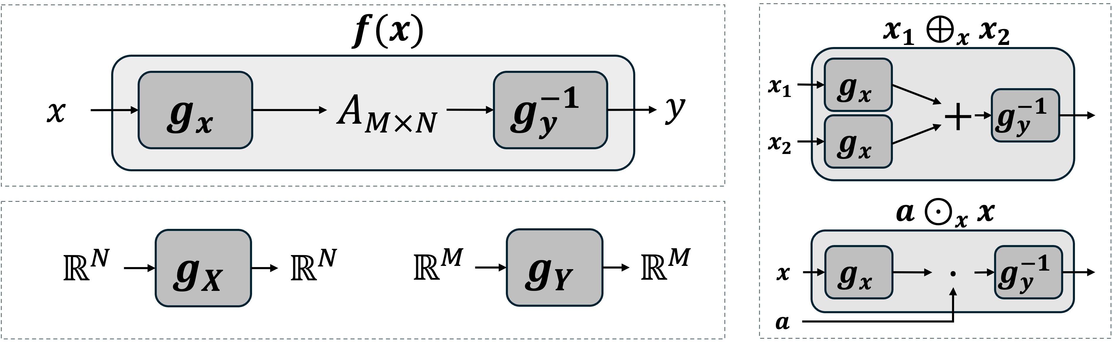
2. Linearizer Framework

Section Summary: The Linearizer framework reimagines how we define linearity in vector spaces, showing that a function which looks nonlinear in everyday math can become perfectly linear by tweaking the rules for adding vectors and scaling them, while keeping the underlying data the same. It works by placing a straightforward linear step, like multiplying by a matrix, between two flexible, reversible neural networks that reshape the input and output spaces. This approach makes it easier to train models, analyze their behavior, and combine them, drawing parallels to simplifying math problems by switching to a better coordinate system.

Linearity is not an absolute concept; it is a property defined relative to a pair of vector spaces, $f:\mathcal{X} \to \mathcal{Y}$. This motivates the use of transport of structure ([4]) to identify a pair of spaces $\mathcal{X}$ and $\mathcal{Y}$, for which a function that is nonlinear over standard Euclidean space is, in fact, perfectly linear. Recall that a vector space is comprised of a set of vectors (e.g. $\mathbb{R}^N$), a field of scalars (e.g., $\mathbb{R}$), and two fundamental operations: vector addition ($+$) and scalar multiplication ($\cdot$). We propose inducing new learnable vector spaces by redefining operations, while keeping vectors and field unchanged.

2.1 Definitions

We introduce a formalism we term Linearizer, in which the relevant vector spaces are immediately identifiable by construction as they are isomorphic to the Euclidean space. The architecture we propose can be trained from scratch or by distillation from an existing model. Our approach is made practical by invertible neural networks [5, 6, 7]. We build our model by wrapping a linear operator, a matrix $A$, between two such invertible networks, $g_x$ and $g_y$:

Definition: Linearizer

Let $\mathcal{X}, \mathcal{Y}$ be two spaces and $g_x:\mathcal{X}\to\mathcal{X}$, $g_y:\mathcal{Y}\to\mathcal{Y}$ be two corresponding invertible functions. Also, let $A:\mathcal{X}\to\mathcal{Y}$ be a linear operator. Then we define the Linearizer $\mathbb{L}_{{g_x, g_y, A}}$ as the following function $f:\mathcal{X}\to\mathcal{Y}$:

$ f(x) = \mathbb{L}_{{g_x, g_y, A}}(x) = g_y^{-1}(A g_x(x)) $

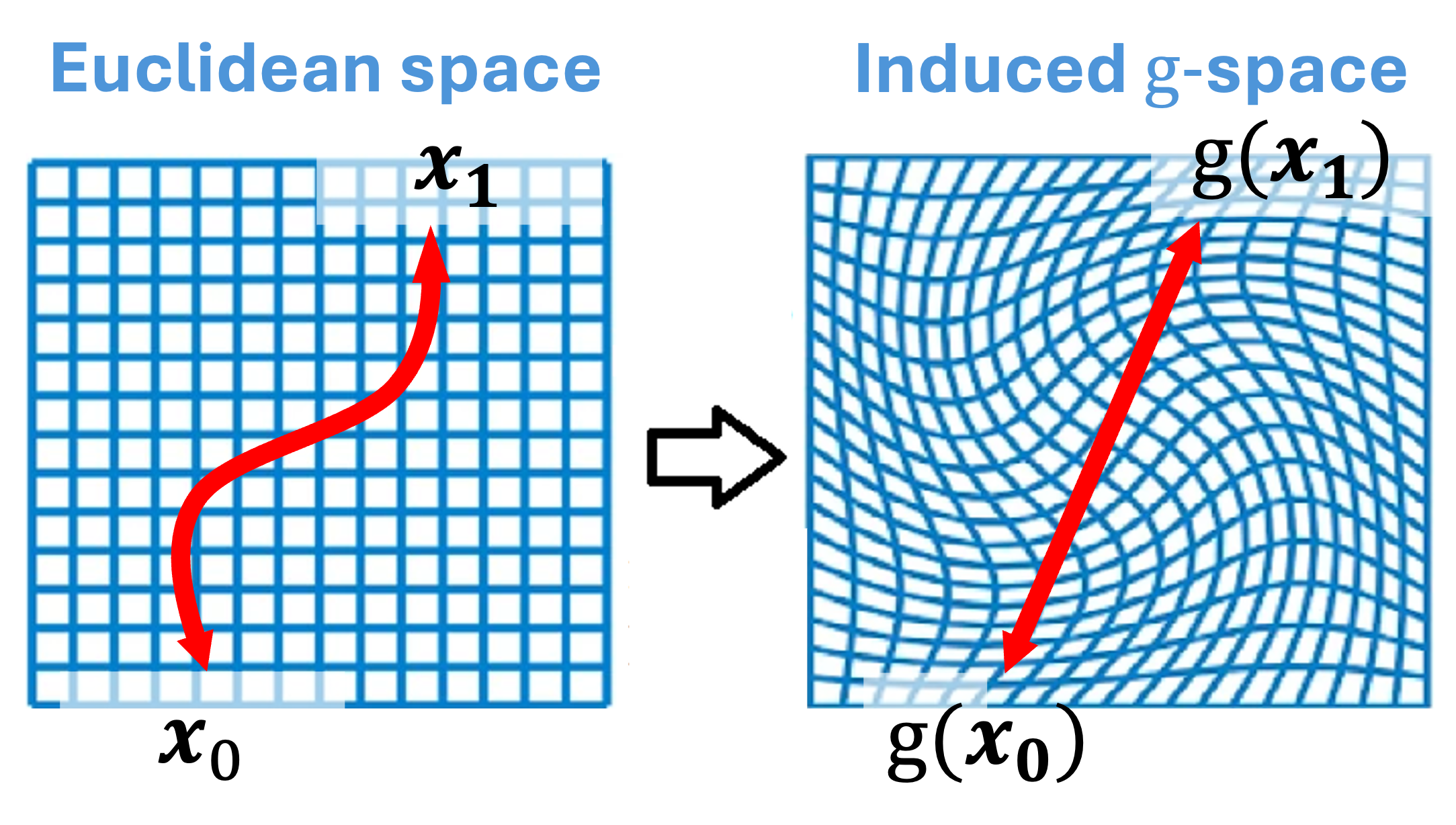
For this construction, we can define the corresponding vector spaces $\mathcal{X}$ and $\mathcal{Y}$, also shown in Figure 1:

Definition: Induced Vector Space Operations

Let $g: V \to V$ be an invertible function. We define a new set of operations, according to the transport of structure, $\oplus$ and $\odot$, for any two vectors $v_1, v_2 \in V$ and any scalar $a \in \mathbb{R}$:

$ \begin{align} v_1 \oplus_g v_2 &:= g^{-1}(g(v_1) + g(v_2)) \ a \odot_g v_1 &:= g^{-1}(a \cdot g(v_1)) \end{align} $

$g_x$, $g_y$, and the core $A$ are learned jointly end-to-end.[^1]

[^1]: Specifically, in our implementation each of $g_x$ and $g_y$ uses 6 invertible blocks (Appendix G.1). The specific INN architecture – affine coupling layers with a tiny U-Net conditioner – is detailed in Appendix G.2 and Appendix G.4. The linear core $A$ is task-specific and its implementations are summarized in Appendix G.3.

2.2 Linearity

The input space $\mathcal{X}$ is defined by operations $(\oplus_x, \odot_x)$ induced by $g_x$, and the output space $\mathcal{Y}$ by $(\oplus_y, \odot_y)$ induced by $g_y$. This is a vector-space isomorphism which promises preservation of geometry.

Proposition 1

$(V, \oplus_g, \odot_g)$ is a vector space over $\mathbb{R}$. This is a direct consequence of the isomorphism. However, we also provide full verification in Appendix A.

Proposition 2

The function $f(x)$ is a linear map from the vector space $\mathcal{X}$ to the vector space $\mathcal{Y}$.

Proof: Linearity is preserved in transport of structure, but we can also verify:

$ \begin{align*} & f(a_1 \odot_x x_1 \oplus_x a_2 \odot_x x_2) && \ & = g_y^{-1}(A g_x(g_x^{-1}(a_1 g_x(x_1) + a_2 g_x(x_2)))) && \ & = g_y^{-1}(a_1 g_y(g_y^{-1}(A g_x(x_1))) + a_2 g_y(g_y^{-1}(A g_x(x_2)))) && \ & = a_1 \odot_y f(x_1) \oplus_y a_2 \odot_y f(x_2) && \blacksquare \end{align*} $

2.3 Intuition

The Linearizer can be understood through several lenses.

Linear algebra analogy.

The Linearizer is analogous to an eigendecomposition or SVD. Just as a matrix is diagonal (i.e. simplest) in its eigenbasis, our function $f$ is a simple matrix multiplication in the "linear basis" defined by $g_x$ and $g_y$. This provides a natural coordinate system in which to analyze and manipulate the function. For example, repeated application of a Linearizer with a shared basis ($g_x=g_y=g$) is equivalent to taking a power of its core matrix:

$ \begin{split} \mathbb{L}{{g, g, A}}^{\circ N}(x) &= \underbrace{f(f(\cdots f}{N \text{ times}}(x))) \ = g^{-1}(A^N \cdot g(x)) &= \mathbb{L}_{{g, g, A^N}}(x) \end{split} $

Geometric interpretation.

$g_x$ can be seen as a diffeomorphism. Equip the input with the pullback metric $g_x^{\ast}\langle\cdot, \cdot\rangle_{\mathbb{R}^N}$ induced by the Euclidean metric in latent space. With respect to this metric, straight lines in latent correspond to geodesics in input, and linear interpolation in the induced coordinates maps to smooth and semantically coherent curves in input space.

2.4 Properties

We review how basic properties of linear transforms are expressed by Linearizers. All these properties follow directly from the vector space isomorphism (transport of structure). Yet, we explicitly derive them separately here.

2.4.1 Composition

Proposition

The composition of two Linearizer functions with compatible spaces $f_1: \mathcal{X} \to \mathcal{Y}$ and $f_2: \mathcal{Y} \to \mathcal{Z}$, is also a Linearizer.

$ \begin{split} (f_2 \circ f_1)(x) &= g_z^{-1}(A_2 g_y(g_y^{-1}(A_1 g_x(x)))) \ &= g_z^{-1}((A_2 A_1) \cdot g_x(x)) \end{split} $

2.4.2 Inner Product and Hilbert Space

Definition 3: Induced Inner Product

Given an invertible map $g:V\to\mathbb{R}^N$, the induced inner product on $V$ is

$ \langle v_1, v_2\rangle_g := \langle g(v_1), g(v_2)\rangle_{\mathbb{R}^N}, $

where the right-hand side is the standard Euclidean dot product.

Equipped with this inner product, the induced vector spaces make Hilbert spaces.

Proposition 4: Induced spaces are Hilbert

Let $g:V \to \mathbb{R}^n$ be a smooth bijection and endow $V$ with the induced vector space operations $(\oplus_g, \odot_g)$ and inner product $\langle u, v\rangle_g ;:=; \langle g(u), , g(v)\rangle_{\mathbb{R}^n}.$ Then $(V, \langle\cdot, \cdot\rangle_g)$ is a Hilbert space.

This is a characteristic of the transport of structure. For explicit proof See Appendix C.

2.4.3 Transpose

Proposition 5: Transpose

Let $f(x)=g_y^{-1}(A g_x(x))$ be a Linearizer.

Its transpose $f^\top:\mathcal{Y}\to\mathcal{X}$ with respect to the induced inner products is

$ f^\top(y) = g_x^{-1} \big(A^\top g_y(y)\big). $

Proof: For all $x\in\mathcal{X}, y\in\mathcal{Y}$,

$ \begin{align} \langle f(x), y\rangle_{g_y} &= \langle A g_x(x), g_y(y)\rangle_{\mathbb{R}^N} = \langle g_x(x), A^\top g_y(y)\rangle_{\mathbb{R}^N} \ &= \langle x, g_x^{-1}(A^\top g_y(y))\rangle_{g_x} = \langle x, f^\top(y)\rangle_{g_x}. \blacksquare \end{align} $

2.4.4 Singular Value Decomposition

Proposition 6: SVD of a Linearizer

Let $A=U\Sigma V^\top$ be the singular value decomposition of $A$.

Then the SVD of $f(x)=g_y^{-1}(A g_x(x))$ is given by singular values $\Sigma$, input singular vectors $\tilde v_i=g_x^{-1}(v_i)$, and output singular vectors $\tilde u_i=g_y^{-1}(u_i)$.

Spectral properties are transferred in isomorphic change of coordinates. We show this explicitly in Appendix B.

3. Theoretical Analysis

Section Summary: The Linearizer model imposes some structural limits, such as requiring its null space to be a full linear subspace, which means it cannot precisely map just a few isolated points to zero without affecting others. However, it remains powerful enough to perfectly fit any finite set of training data by cleverly placing these constraints outside the data itself, enabling good performance on real-world high-dimensional inputs like images that lie on simpler underlying patterns. The core matrix A primarily sets the function's rank when input and output networks differ, but plays a bigger role in shaping eigenvalues when they are the same; in practice, keeping A as a full matrix is essential for creating diverse families of models, such as those used in step-by-step processes like flow matching, where a simpler diagonal form would limit flexibility.

Before demonstrating applications, we address two fundamental theoretical questions: the expressive capacity of the Linearizer and the functional necessity of the core matrix.

3.1 Expressiveness

A natural concern is whether enforcing a linear bottleneck restricts the model's capacity. Strictly speaking, the architecture does impose topological constraints on the global function $f$. For example, the kernel (null space) of $f$ is determined entirely by the kernel of $A$. Since linear subspaces are either trivial or infinite-dimensional, a Linearizer cannot, for instance, map exactly three distinct points to zero while mapping a fourth point to non-zero, as this would violate the subspace properties of the kernel in the latent space.

Despite this topological constraint,

we prove that the Linearizer is expressive enough to fit any finite training set. In Appendix Theorem 11 (Theorem H.4), we formally prove that for any finite dataset ${(x_i, y_i)}_{i=1}^N$, there exist invertible networks $g_x, g_y$ and a linear map $A$ such that the Linearizer satisfies $f(x_i) = y_i$ to arbitrary precision.

How can the model be topologically constrained yet fit any dataset? The resolution lies in the degrees of freedom available outside the data support. For example, the required infinite null-space can lie outside of the data. This logic also applies to infinite continuous manifolds of lower dimension than the space, allowing generalization on high-dimensional data, such as images or text embeddings that often reside on a low-dimensional manifold

3.2 On the Role of the Core Operator A

Given the power of $g$, what is the role of the matrix $A$? We analyze this in two regimes.

The General Regime ($g_x \neq g_y$). Let the SVD of $A$ be $U\Sigma V^T$. In the general case where $g_x$ and $g_y$ are distinct, we could define new invertible networks $g'_y = g_y \circ U$ and $g'_x = V^T \circ g_x$. The function would then be $f(x) = (g'_y)^{-1}(\Sigma g'_x(x))$. If we further allow the networks to absorb the scaling defined by the singular values in $\Sigma$, then the core operator could be reduced to a diagonal matrix of zeros and ones (note that this does not imply idempotency unless $g_x=g_y$). In this sense, the fundamental role of $A$ is simply to define the rank of the function $f$.

The Constrained Regime ($g_x = g_y = g$). In applications like Flow Matching or Idempotency, the input and output spaces are identical so $g_x = g_y$. Here, the two networks are not independent. To preserve the structure $f(x)=g^{-1}(A g(x))$, any transformation absorbed by $g$ must be inverted by $g^{-1}$. This rules out $g$ absorbing SVD elements $U, V$ as they are not necessarily mutual inverses. For diagonalizable matrices however, eigen-decomposition can be applied. Then, $A = Q\Lambda Q^{-1}$, where one could define $g' = Q^{-1} \circ g$ and $f(x) = (g')^{-1}(\Lambda g'(x))$. Here, $A$ determines the function's eigenvalues—a stronger role than just its rank—but this is

Practical Necessity: Functional Diversity. Does the above analysis suggest that we can always use a diagonal $A$? Crucially, this analysis only applies to learning a single static function. However, our applications typically utilize "families" of Linearizers, that share the same $gx, gy$ with different $A$ matrices. For example our flow-matching application employs a different A for each timestep. The expressiveness inside such family is dictated by the expressiveness of $A$ which would be significantly reduced if it were diagonal.

4. Applications

Section Summary: This section explores practical applications of the framework, starting with one-step flow matching, a technique that trains a neural network to quickly transform random noise into realistic data like images, bypassing the slow, multi-step process of traditional methods. By using their Linearizer model, which simplifies paths in a hidden space, the approach collapses complex calculations into a single efficient operation, enabling fast generation without losing quality. Tests on datasets like handwritten digits and celebrity faces show that one-step results match multi-step ones closely, and the method also supports reversing the process to edit or interpolate images, addressing limitations in similar AI tools.

Having established the theoretical foundations, we now present proof-of-concept applications that highlight advantages of our framework, leaving scaling and engineering refinements for future work.

4.1 One-Step Flow Matching

Flow matching ([8, 9]) trains a network to predict the velocity field that transports noise samples to data points. In our setting, diffusion models [10] and flow matching [8] are, from an algorithmic standpoint, equivalent under standard assumptions [11]; hence we use the two frameworks interchangeably. Traditionally, this velocity must be integrated over time with many small steps, making generation slow. We train flow matching using our Linearizer as the backbone, with a single vector space ($g_x=g_y=g$). The key property that helps us achieve one-step generation is the closure of linear operators. Applying the model sequentially with some simple linear operations in between steps is a chain of linear operations. This chain can be collapsed to a single linear operator so that the entire trajectory is realized in a single step.

Training.

Training is just as standard FM, only using the Linearizer model and the induced spaces. We define the forward diffusion process:

$ x_t = (1-t) \odot x_0 \oplus t \odot x_1 = g^{-1} \bigl((1-t), g(x_0) + t, g(x_1)\bigr). $

This is a straight line in the $g$-space, mapped back to a curve in the data space. The target velocity is

$ v = x_1 \ominus x_0 = g^{-1} \bigl(g(x_1)-g(x_0)\bigr). $

We parameterize a time-dependent Linearizer

$ f(x_t, t) = g^{-1}(A_t g(x_t)), $

and train it to predict $v$. The loss is

$ \begin{split} \mathcal{L} &= \mathbb{E}{x_0, x_1, t}, \bigl|, v \ominus f(x_t, t) , \bigr|^2 \ &= \mathbb{E}{x_0, x_1, t}, \bigl|, g^{-1}\Bigl(g(x_1)-g(x_0) - A_t g(x_t)\Bigr), \bigr|^2 \end{split} $

This objective ensures that the learned operators $A_t$ approximate the true velocity of the flow within the latent space of the Linearizer.

Sampling as a collapsed operator.

In inference time, standard practice is to discretize the ODE with many steps. In the induced space, an Euler update reads

$ x_{t+\Delta t} = x_t \oplus \bigl(\Delta t \odot f(x_t, t)\bigr), $

which expands to

$ g(x_{t+\Delta t}) = (I + \Delta t, A_t), g(x_t). $

Iterating this $N$ times produces

$ g(\hat{x}1) \approx \underbrace{\Bigl[\prod{i=0}^{N-1}(I + \Delta t, A_{t_i})\Bigr]}_{:=B} g(x_0). $

The entire product can be collected into a single operator $B$, resulting in

$ \hat{x}_1 = g^{-1}(B g(x_0)). $

Thus, what was originally a long sequence of updates collapses into a single multiplication. In practice, higher-order integration such as Runge–Kutta ([12, 13]) may be used to calculate $B$ more accurately (see Appendix F). $B$ is calculated only once, after training. Then generation requires only a single feedforward activation of our model on noise, regardless of the number of steps discretizing the ODE.

Geometric intuition.

$g$ acts as a diffeomorphism: in its latent space, the path between $x_0$ and $x_1$ is a straight line, and the velocity is constant. When mapped back to the data space via $g^{-1}$, this straight line becomes a curved trajectory. The Linearizer exploits this change of coordinates so that, in the right space, the velocity field is trivial, and the expensive integration disappears.

Implementation.

The operator $A$ is produced by an MLP whose input is $t$. To avoid huge matrix multiplications we build $A$ as a low-rank matrix, by multiplying two rectangular matrices. $g$ does not take $t$ as input. Full implementation details are provided in App. Appendix G.

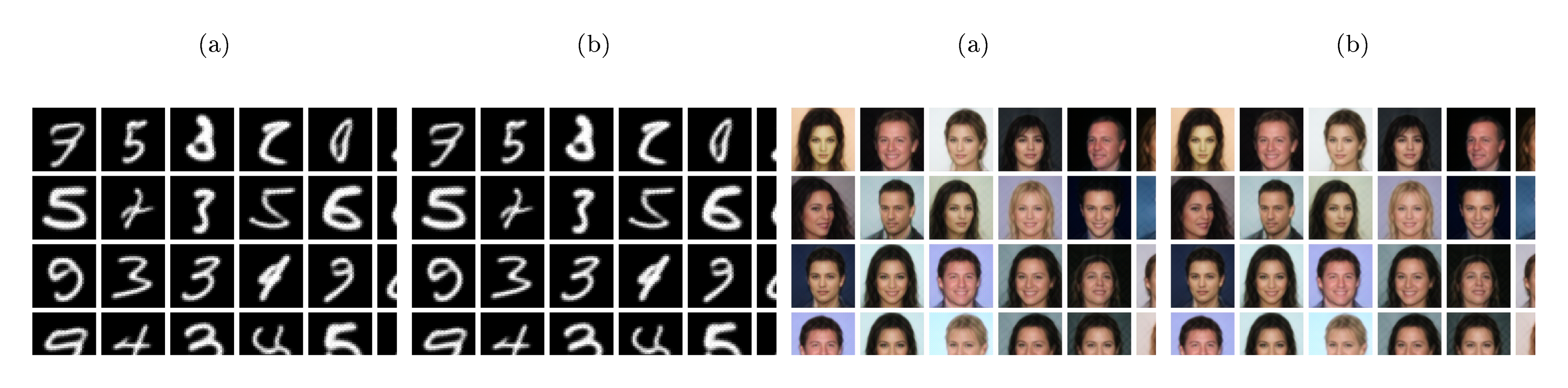
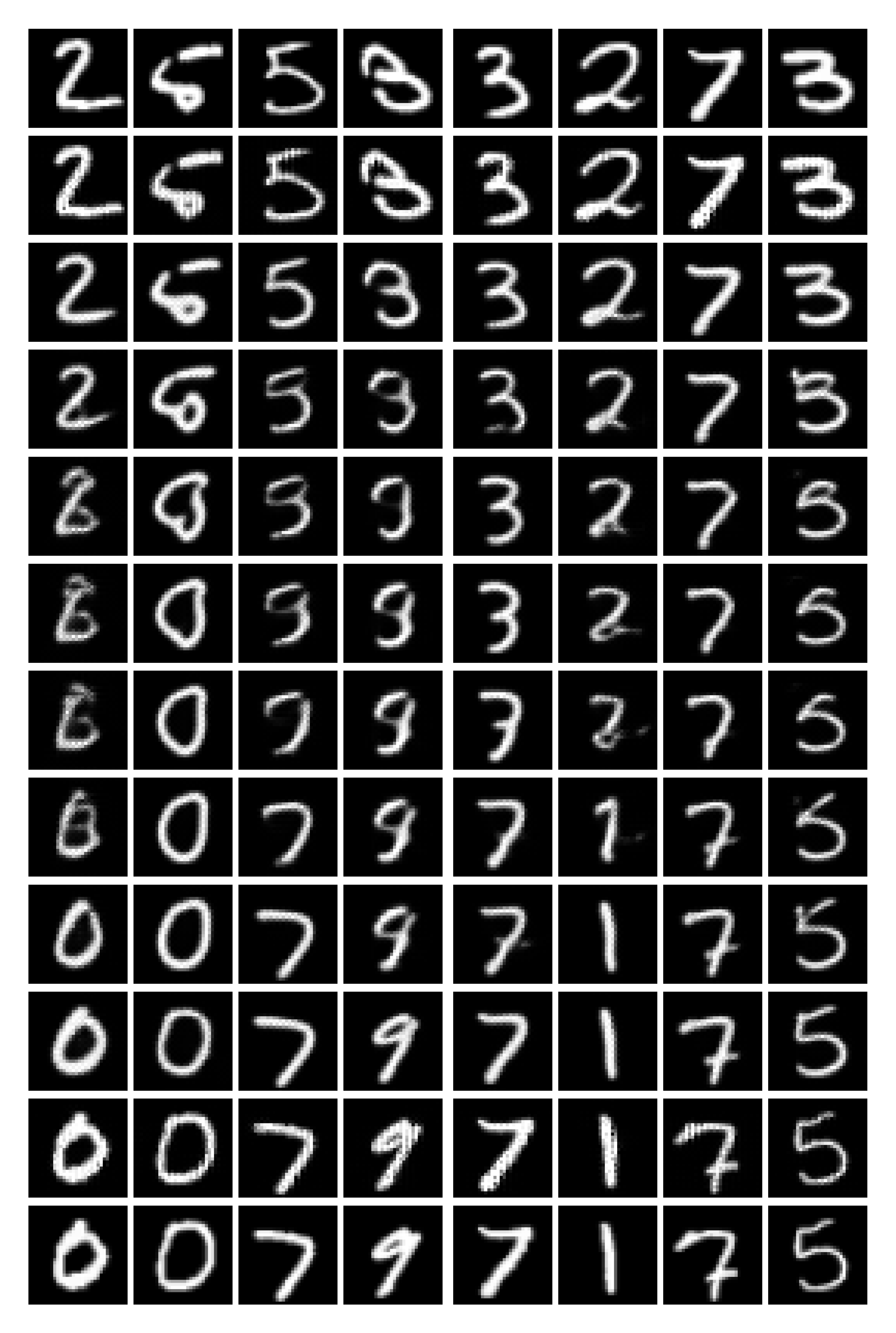
One-step generation.

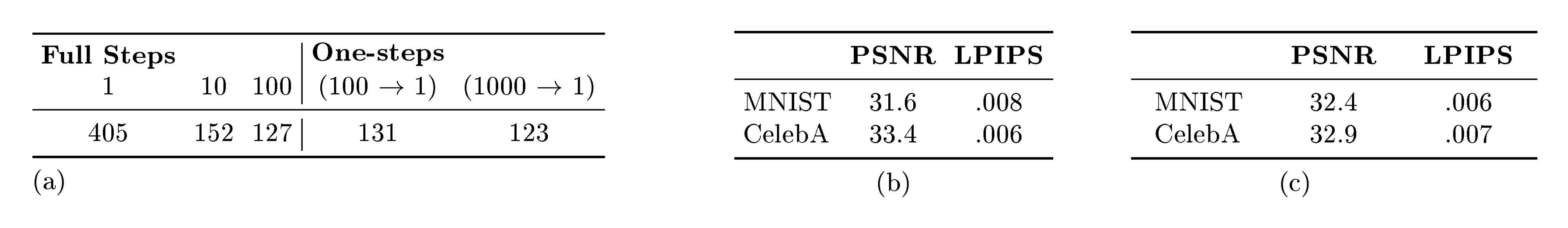
Figure 2 shows qualitative results on MNIST [14] (32 $\times$ 32) and CelebA [15] (64 $\times$ 64). As discussed, our framework supports both multi-step and one-step sampling and yields effectively identical outputs. Visually, the samples are indistinguishable across datasets; quantitatively, the mean squared error between one-step and multi-step generations is $\mathbf{3.0\times 10^{-4}}$, confirming their near-equivalence in both datasets. Additionally, we evaluate FID across different step counts and our one-step simulation (see Figure 4 (a)). The FID from 100 full iterative steps closely matches our one-step formulation, empirically validating the method's theoretical guarantee of one-step sampling. Moreover, simulating more steps (1000 $\to$ 1 vs. 100 $\to$ 1) improves FID by $\sim$ 8 points, highlighting the strength of the linear-operator formulation. Furthermore, we validate one-step vs. 100 step fidelity, showing high similarity as presented in Figure 4(c). Finally, while our absolute FID is not yet competitive with state-of-the-art systems, our goal here is to demonstrate the theory in practice rather than to exhaustively engineer for peak performance; scaling left to future work.

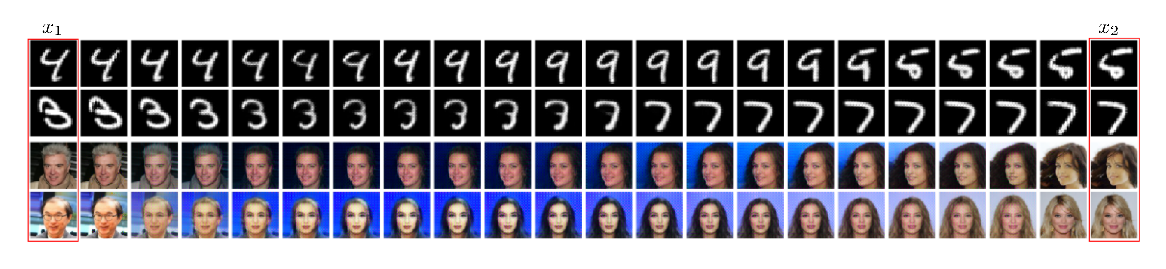
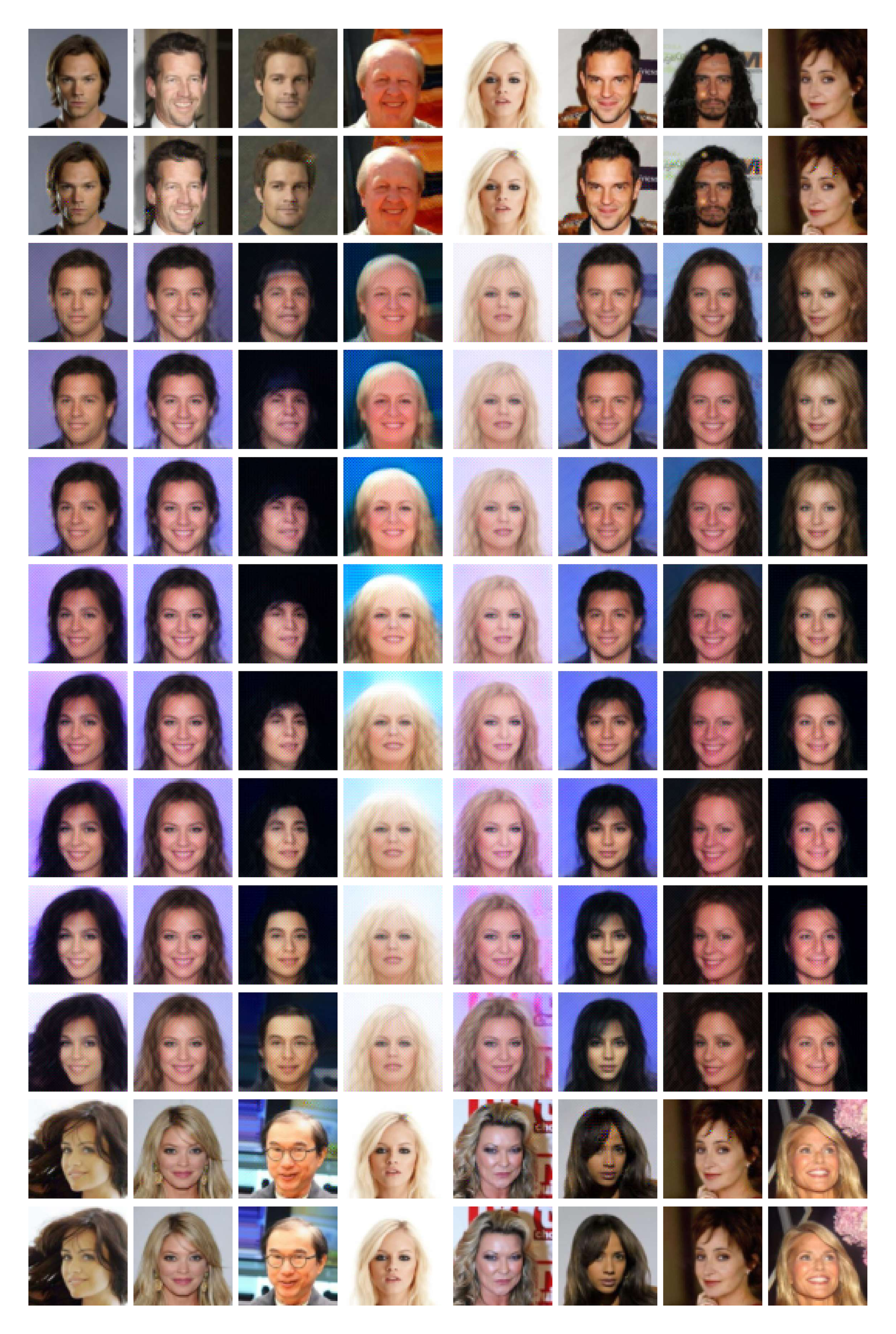
Inversion and interpolation.

A fundamental limitation of flow models is that, in contrast to VAEs ([16]), they lack a natural encoder: they cannot map data back into the prior (noise) space, and thus act only as decoders. As a result, inversion methods for diffusion ([17, 18, 19]) have become an active research area. However, these techniques are approximate and often suffer from reconstruction errors, nonuniqueness, or computational overhead. Our framework connects diffusion-based models with encoding ability.

Because the Linearizer is linear, its Moore–Penrose pseudoinverse is also a Linearizer:

Lemma 7: Moore–Penrose pseudoinverse of a Linearizer

The Moore–Penrose pseudoinverse of $f$ with respect to the induced inner products is

$ f^\dagger(y) = g_x^{-1}(A^\dagger g_y(y)) $

Proof: We verify the four Penrose equations ([20]) in Appendix D.

This property enables the exact encoding of data in the latent space. For example, given two data points $x_1, x_2$, we can encode them via $z^{a} = (1-a), f^\dagger(x_1) ;+; a, f^\dagger(x_2), $ and decode back by $\hat{x}^{a} = f(z^{a}).$ Figure 3 shows latent interpolation between two real (non-generated) images. Additionally, we evaluate reconstruction quality using two standard metrics: LPIPS [21] and PSNR. Figure 4(b) shows inversion-reconstruction consistency. Our results confirm high-quality information preservation.

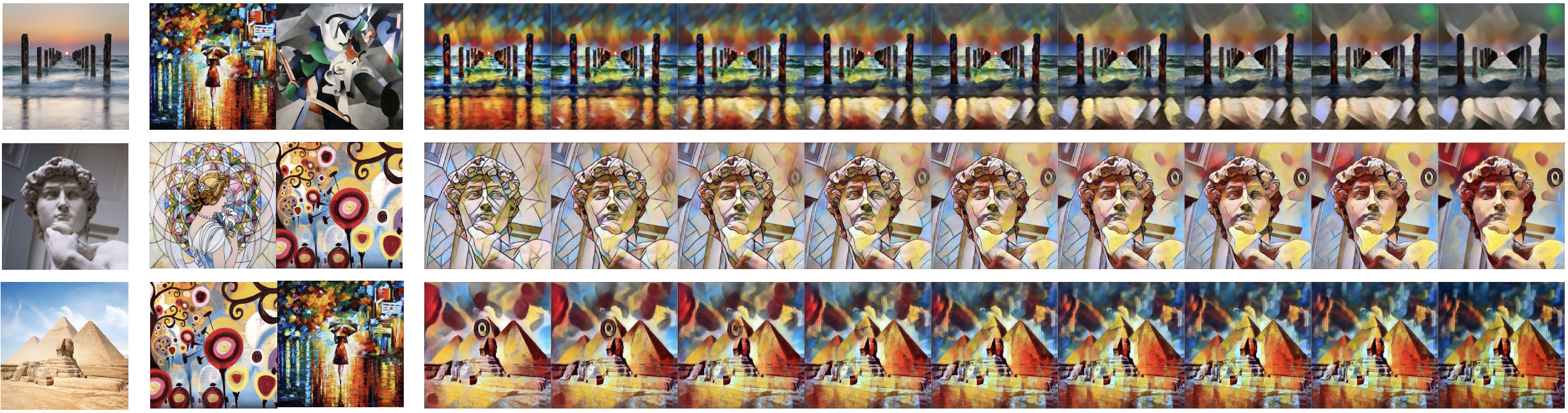
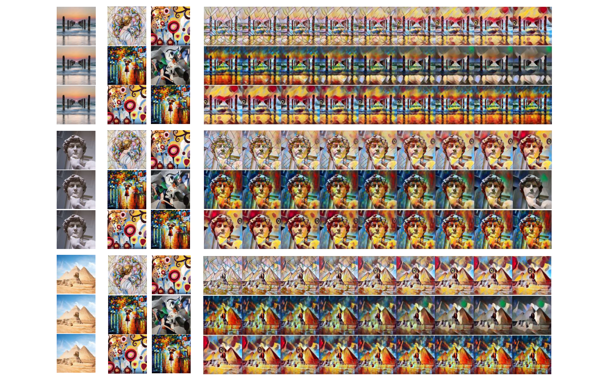
4.2 Modular Style Transfer

Style transfer has been widely studied since [22] proposed optimizing image pixels to match style and content statistics. [23] introduced perceptual-loss training of feed-forward networks, making style transfer practical.

Linearizer formulation.

We fix $g_x$ and $g_y$ and associate each style with a matrix $A_{\text{style}}$. The matrix $A_{\text{style}}$ is produced by a hypernetwork that takes a style index as input (rather than time, as in the one-step setting). Then

$ f_{\text{style}}(x) = g_y^{-1}(A_{\text{style}} g_x(x)). $

This separates content representation from style, making styles modular and algebraically manipulable. In practice, we distill $A_{\text{style}}$ from a pretrained Johnson-style network.

Style interpolation.

Given two trained style operators, $A_{\text{style}}^{x}$ and $A_{\text{style}}^{y}$, we form an interpolated operator $A_{\text{style}}^{(\alpha x + (1-\alpha) y)}$ that represents a linear interpolation between them. We evaluated $\alpha \in {0, , 0.35, , 0.40, , 0.45, , 0.50, , 0.55, , 0.60, , 0.65, , 1}$,

$ f_{\text{style}}^{(\alpha x + (1-\alpha) y)}(x) = g_y^{-1} \left(A_{\text{style}}^{(\alpha x + (1-\alpha) y)}, g_x(x)\right), $

with results shown in Figure 5. Rows 1–3 interpolate between mosaic/candy, rain-princess/udnie, and candy/rain-princess, respectively. See App. Appendix E for additional transfers.

4.3 Linear Idempotent Generative Network

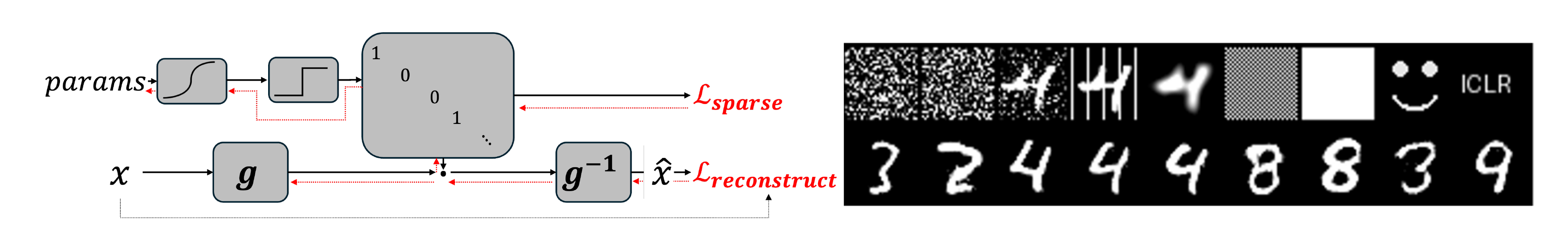
Idempotency, $f(f(x))=f(x)$, is a central concept in algebra and functional analysis. In machine learning, it has been used in Idempotent Generative Networks (IGNs) ([24]), to create a projective generative model. It was also used for robust test time training ([25]). Enforcing a network to be idempotent is tricky and is currently done by using sophisticated optimization methods such as ([26]). The result is only an approximately idempotent model over the training data. We demonstrate enforcing accurate idempotency through architecture using our Linearizer. The key observation is that idempotency is preserved between the inner matrix $A$ and the full function $f$.

Lemma

The function $f$ is idempotent $\iff$ The matrix $A$ is idempotent.

Proof: For all $x$,

$ \begin{aligned} A^2 = A &;\iff; g^{-1} \big(A^2 g(x)\big) = g^{-1} \big(A g(x)\big) \ &;\iff; \big{, g^{-1} \circ A \circ \underbrace{(g\circ g^{-1})}_{\mathrm{Id}}\circ A \circ g, \big}(x) \ &\quad;= \big{, g^{-1} \circ A \circ g, \big}(x) \ &;\iff; f(f(x)) = f(x) \ &\quad;\text{(by the definition of $f$)} \blacksquare \end{aligned} $

Method.

Figure 6 left shows the method. Recall that idempotent (projection) matrices have eigenvalues that are either $0$ or $1$. We assume a diagonalizable projection matrix $A=Q\Lambda Q^{-1}$ where $\Lambda$ is a diagonal matrix with entries ${0, 1}$. The matrices $Q, Q^{-1}$ can be absorbed into $g, g^{-1}$ without loss of expressivity. So we can train a Linearizer $g^{-1}(\Lambda g(\cdot))$. In order to have $\Lambda$ that is binary yet differentiable, we use an estimation ([27]) having underlying probabilities $P$ as parameters in $[0, 1]$ and then use $A = \text{round}(P) + P - P.\text{detach}()$ where detach means stopping gradients. We forward propagate rounded values ($0$ or $1$) and back propagate continuous values.

Idempotency by architecture allows reducing the idempotent loss used in [24]. We need the data to be fixed points with the tightest possible latent manifold. The losses are:

$ \begin{align} \mathcal{L}{\text{rec}} &= |f(x)-x|^2\ \mathcal{L}{\text{sparse}} &= \frac{1}{N} \text{Rank}(A) = \frac{1}{N}\sum_i^N \lambda_i \end{align} $

We further enforce regularization that encourages $g$ to preserve the norms:

$ \begin{align} \mathcal{L}_{\text{isometry}} &= \Bigl\lVert\lVert g(x)-g(0)\rVert^2-\lVert x\rVert^2\Bigr\rVert_1 \end{align} $

This nudges $g$ towards a near-isometry around the data, thus resisting mapping far-apart inputs to close outputs. It mitigates collapse and improves stability. We apply it with a small weight ($0.001$).

From local to global projectors.

As [24] put it, "We view this work as a first step towards a global projector." In practice, IGNs achieve idempotency only around the training data: near the source distribution or near the target distribution they are trained to reproduce. If you venture further away, then the outputs degenerate into arbitrary artifacts not related to the data distribution. In contrast, our Linearizer is idempotent by architecture. It does not need to be trained to approximate projection, it is one. Figure 6 right shows various inputs projected by our model onto the distribution. Interestingly, there is not even a notion of a separate source distribution: we never inject latent noise during training, and in a precise sense the entire ambient space serves as the source. This makes our construction a particularly unusual generative model and a natural next step toward the global projector envisioned in [24].

4.4 Additional Experiments

We provide more experiments of diverse types of data and tasks to empirically test the robustness of the Linearizer and its ability to learn various mappings.

CelebFaces Attributes (CelebA).

We evaluate on the CelebA face-attribute classification task, which includes large pose variation, background clutter, diverse identities, and rich annotations (40 binary attributes such as Male, Eyeglasses, Blond Hair). After training, our Linearizer attains a test accuracy of 87.6%; for reference, a ResNet-50 baseline reaches 86.1%. These results suggest that the Linearizer handles moderately complex, real-world visual variability.

Distillation of nonlinear disentanglement models.

In this experiment, we distill the encoder of a pretrained disentanglement model into a Linearizer (using pretrained checkpoints). We consider VAE, FactorVAE, and $\beta$-VAE on the dSprites dataset, which provides ground-truth factors of variation. We assess quality with standard metrics: FactorVAE, SAP, and DCI (disentanglement, completeness, informativeness). Across models, the Linearizer closely matches the original encoders (rows prefixed with Linearizer-) on these metrics (often slightly improving FactorVAE/SAP, e.g., BetaH: +0.10/+0.01), indicating that it can capture highly nonlinear transformations with no loss in disentanglement quality of the encoded representations. For the table with full results please see Appendix E.3.

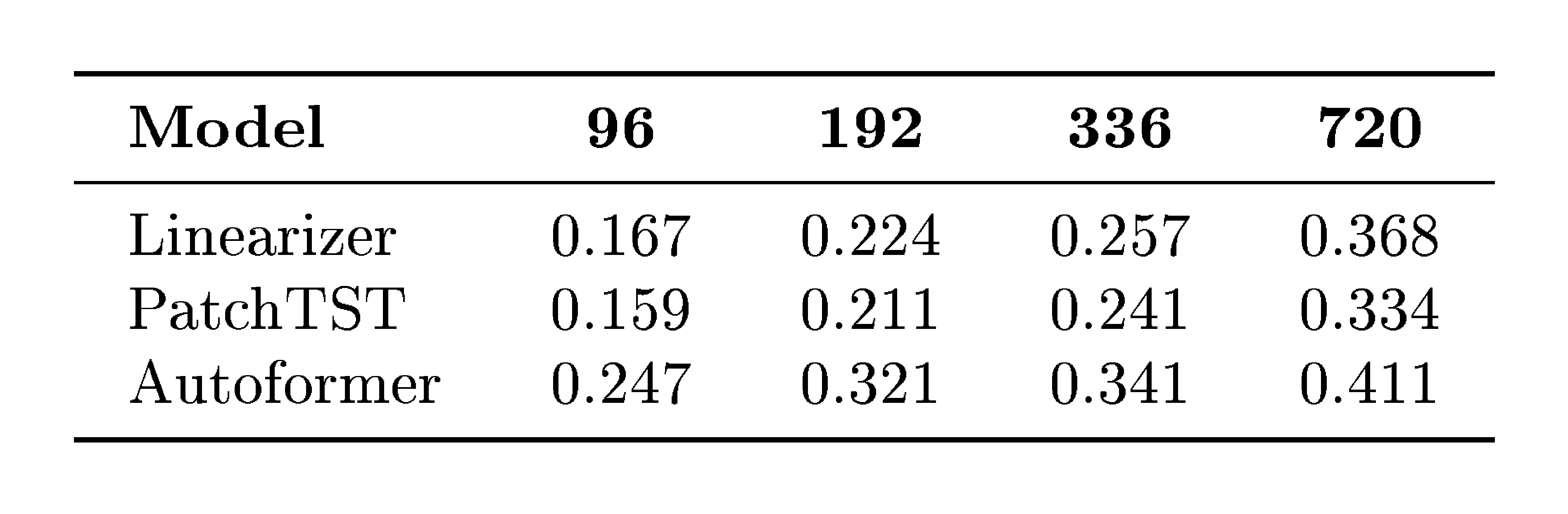
Weather Prediction.

To further explore the applicability of our framework, we conduct a small experiment in a new domain: regression of future steps. We use a standard weather-prediction benchmark where the model must predict the future given 96 past time steps. We compare our method with two well-known baselines tailored for regression, Autoformer [28] and PatchTST [29]. Briefly, although our method is generic, it shows competitive results, surpassing the highly nonlinear Autoformer and being comparative (e.g., gaps of $\sim$ 0.008–0.034 MSE depending on horizon) with the strong PatchTST baseline. For the table with full results please see Appendix E.3.

5. Limitations

Section Summary: The Linearizer offers a structured way to make neural networks' mappings exactly linearizable, but it still has some key drawbacks. Invertible networks like this are tougher to train than typical ones and require extra careful planning. While the approach shows promise in early tests, it hasn't been scaled up to compete with the best current standards, and questions remain about its full theoretical capabilities.

While the Linearizer introduces a principled framework for exact linearization of neural maps, several limitations remain. First, invertible networks are inherently more challenging to train than standard architectures, often requiring careful design. Second, this work represents a broad and general first step: our applications demonstrate feasibility, but none are yet scaled to state-of-the-art benchmarks. Finally, the precise expressivity of the Linearizer remains an open theoretical question.

6. Related Work

Section Summary: This section reviews how the paper's Linearizer approach, which uses invertible neural networks to transform arbitrary mappings into exact finite-dimensional linear forms for easier algebraic manipulation, relates to existing methods in dynamical systems and machine learning. It contrasts with Koopman theory's approximations of nonlinear dynamics and the Neural Tangent Kernel's parameter-space linearity by achieving direct input-output linearity in learned coordinates, even for networks of any width, and differs from one-step diffusion distillation techniques by training from scratch to support tasks like composition and inversion. Unlike invertible networks for density modeling, equivariant representations for symmetries, manifold-flattening for data geometry, or normalizing flows for distributions, the Linearizer focuses on simplifying mapping functions themselves through nonlinear coordinate changes while preserving expressiveness.

Linearization in Dynamical Systems.

Koopman theory linearizes nonlinear dynamics via observables, yielding $z_{t+1}=K z_t$ (discrete) or $\dot z = A z$ (continuous) ([30]). Data-driven realizations such as DMD and EDMD construct finite-dimensional approximations of this infinite-dimensional operator on a chosen dictionary of observables, which typically produces a square matrix because the dictionary is mapped into itself, although variants with different feature sets exist ([31, 32, 33]). Linear algebraic analyses such as SVD, eigendecomposition, and taking powers are standard in these Koopman approximations. Our work addresses a different object: an arbitrary learned mapping $f:\mathcal{X}\to\mathcal{Y}$. We learn invertible coordinate maps $g_x$ and $g_y$ and a finite matrix $A$ such that $g_y \circ f \circ g_x^{-1} = A$, which gives the exact finite-dimensional linearity of $f$ between induced spaces. This formulation allows for distinct input and output coordinates, allows $A$ to be rectangular when $\dim\mathcal{X}\neq\dim\mathcal{Y}$, and transfers linear-algebraic structure in $A$ directly to $f$ in a controlled way. One can compute $\mathrm{SVD}(f)$ via $\mathrm{SVD}(A)$, invert analytically with $A^{+}$, impose spectral constraints (e.g., idempotency) via $\sigma(A)$, and more.

Neural Tangent Kernel.

The NTK framework shows that infinitely wide networks trained with small steps evolve linearly in parameter space ([34]). However, the resulting model remains nonlinear in input-output mapping. In comparison, our contribution achieves input-output linearity in a learned basis for any network width, independent of training dynamics.

One-Step Diffusion Distillation.

Reducing sampling cost in diffusion models often uses student distillation: Progressive Distillation ([35]), Consistency Models ([36]), Distribution Matching Distillation (DMD) and f-distillation fall into this category. A recent work, the Koopman Distillation Model (KDM) ([37]), uses Koopman-based encoding to distill a diffusion model into a one-step generator, achieving strong FID improvements through offline distillation. The Koopman Distillation Model (KDM) distills a pre-trained diffusion teacher into an encoder-linear-decoder for diffusion only. We train from scratch, enforce exact finite-dimensional linearity by construction, and target multiple use cases including composition, inversion, idempotency, and continuous evolution. Unlike some invertible Koopman setups that force a shared map, KDM employs distinct encoder components and a decoder and does not enforce $g_x = g_y$.

Invertible Neural Networks.

Invertible models like NICE ([6]), RealNVP ([7]) and Glow ([38]) use invertible transforms for density modeling and generative sampling. In this work, we make use of such invertible neural networks to impose a bijective change of coordinates that allows linearity (Proposition 2 only holds given this invertibility of $g_x$, $g_y$) rather than modeling distribution.

Group-theoretic and Equivariant Representations.

Let $G$ act on $\mathcal{X}$ via $(g, x)\mapsto g\cdot x$. Many works learn an encoder $e:\mathcal{X}\to V$ and a linear representation $\rho:G\to \mathrm{GL}(V)$ such that the equivariance constraint $e(g\cdot x)=\rho(g), e(x)$ holds approximately, often with a decoder $d$ that reconstructs $x$ or enforces $d(\rho(g)z)\approx g\cdot d(z)$ ([39]). The objective is to make the action of a symmetry group linear in latent coordinates. In contrast, we target a different object: an arbitrary learned map $f:\mathcal{X}\to\mathcal{Y}$. We construct invertible $g_x, g_y$ and a finite matrix $A$ so that $g_y\circ f\circ g_x^{-1}=A$, which yields exact finite-dimensional linearity of $f$ between induced spaces and enables direct linear algebra on $f$ via $A$.

Manifold Flattening and Diffeomorphic Autoencoders.

Manifold-flattening methods assume data lie on a manifold $M\subset\mathbb{R}^N$ and learn or construct a map $\Phi:\mathbb{R}^N\to\mathbb{R}^k$ so that $\Phi(M)$ is close to a linear subspace $L$, often with approximate isometry on $M$ ([40]). Diffeomorphic autoencoders parameterize deformations $\varphi\in\mathrm{Diff}(\Omega)$ with a latent $z$ in a Lie algebra and use a decoder to warp a template, with variants using a log map to linearize the deformation composition ([41]). These approaches flatten data geometry or deformation fields, whereas our Linearizer flattens a mapping function rather than a manifold or deformation group.

Deep Linear Networks.

Networks composed solely of linear layers are linear in the Euclidean basis and are primarily used to study optimization paths ([42, 43, 44]). They lack expressive power in standard coordinates. In contrast, our Linearizer is expressive thanks to $g_x$ and $g_y$ that are nonlinear over the standard vector spaces, yet maintains exact linearity in the induced coordinate system.

Normalizing Flows.

Normalizing flows [5] use invertible networks to map Gaussians to complex data distributions, preserving density via the change-of-variables formula. Linearizers use the same building block, an invertible network, but instead of transporting measures, they transport algebraic structure. In this sense, Linearizers may be viewed as the "linear-algebraic analogue" of normalizing flows: both frameworks exploit invertible transformations to pull back complex objects into domains where they become simple and tractable.

7. Conclusion

Section Summary: The Linearizer is a new framework that teaches neural networks to perform exact linear operations in a transformed space, enabling innovative uses like efficient one-step image generation, flexible style transfers in art or design, and ensuring certain network behaviors repeat reliably. Looking forward, researchers aim to expand this to handle bigger datasets and sharper images for faster AI creation tools, and to model real-world movements over time using math tricks like matrix exponentials for simulations in physics or video. Ultimately, exploring the full power of Linearizer and combining it with other AI techniques promises exciting advances in how machines learn complex patterns.

We introduced the Linearizer, a framework that learns invertible coordinate transformations such that neural networks become exact linear operators in the induced space. This yields new applications in one-step flow matching, modular style transfer, and architectural enforcement of idempotency. Looking ahead, several directions stand out. First, scaling one-step flow matching and IGN to larger datasets and higher resolutions could provide competitive generative models with unprecedented efficiency. Second, the matrix structure of the Linearizer opens the door to modeling motion dynamics: by exploiting matrix exponentials, one could simulate continuous-time evolution directly, extending the approach beyond generation to physical and temporal modeling. More broadly, characterizing the theoretical limits of Linearizer expressivity, and integrating it with other operator-learning frameworks, remains an exciting avenue for future research.

Impact Statement

Section Summary: This paper introduces a new framework for neural networks that improves their theoretical foundations and makes them more efficient to run. It mainly aims to speed up generative AI models, like those that create images or text through a step-by-step diffusion process, allowing them to produce results in just one step instead of many. This cuts down on computing power and energy use, but it carries the usual risks of generative AI, such as generating fake or deceptive content, without adding any fresh ethical issues to the field.

This paper presents a fundamental architectural framework intended to advance the theoretical understanding and computational efficiency of neural networks. A primary application of our work is accelerating generative diffusion models via one-step sampling. While this offers significant benefits in terms of reduced computational cost and energy consumption during inference, it shares the general societal risks associated with generative AI, such as the potential for creating misleading synthetic content. We believe our specific method does not introduce new ethical concerns beyond those already established in the field of generative modeling.

Appendix

Section Summary: This appendix provides mathematical proofs for three key propositions in the context of vector spaces and linear algebra. The first proof demonstrates that a set equipped with custom addition and scalar multiplication operations, derived from a bijective mapping to Euclidean space, satisfies all the axioms required to form a valid vector space over the real numbers. The second proof shows how to compute the singular value decomposition (SVD) of a linear transformation between two spaces by leveraging the SVD of an underlying matrix and invertible mappings that preserve inner products, ensuring the result holds in the induced Hilbert spaces. The third proof establishes that such a set, with an induced inner product from the mapping, becomes a complete Hilbert space, isomorphic to standard Euclidean space.

A. Proof of Proposition 1 (Valid Vector Spaces)

Proof: We verify that $(V, \oplus_g, \odot_g)$ is a vector space over $\mathbb{R}$ by transporting each axiom via $g$ and $g^{-1}$, using only the definitions

$ u\oplus_g v := g^{-1}(g(u)+g(v)), \qquad a\odot_g u := g^{-1}(a, g(u)). $

For $u, v, w\in V$ and $a, b\in\mathbb{R}$:

1. Closure

$ u\oplus_g v ;=; g^{-1} \big(g(u)+g(v)\big) ;\in; V. $

2. Associativity

$ \begin{aligned} (u\oplus_g v)\oplus_g w &= g^{-1} \big(g(u\oplus_g v)+g(w)\big) \ &= g^{-1} \big((g(u)+g(v))+g(w)\big) \ &= g^{-1} \big(g(u)+(g(v)+g(w))\big) \ &= g^{-1} \big(g(u)+g(v\oplus_g w)\big) \ &= u\oplus_g (v\oplus_g w). \end{aligned} $

3. Commutativity

$ \begin{aligned} u\oplus_g v &= g^{-1} \big(g(u)+g(v)\big) \ &= g^{-1} \big(g(v)+g(u)\big) \ &= v\oplus_g u. \end{aligned} $

4. Additive identity (with $0_V:=g^{-1}(0)$)

$ \begin{aligned} u\oplus_g 0_V &= g^{-1} \big(g(u)+g(0_V)\big) = g^{-1} \big(g(u)+0\big) = u. \end{aligned} $

5. Additive inverse (with $(-u):=g^{-1}(-g(u))$)

$ \begin{aligned} u\oplus_g (-u) &= g^{-1} \big(g(u)+g(-u)\big) = g^{-1} \big(g(u)-g(u)\big) = g^{-1}(0) = 0_V. \end{aligned} $

6. Compatibility of scalar multiplication

$ \begin{aligned} a\odot_g (b\odot_g u) &= g^{-1} \big(a, g(b\odot_g u)\big) = g^{-1} \big(a, (b, g(u))\big) \ &= g^{-1} \big((ab), g(u)\big) = (ab)\odot_g u. \end{aligned} $

7. Scalar identity

$ \begin{aligned} 1\odot_g u &= g^{-1} \big(1\cdot g(u)\big) = g^{-1} \big(g(u)\big) = u. \end{aligned} $

8. Distributivity over vector addition

$ \begin{aligned} a\odot_g (u\oplus_g v) &= g^{-1} \big(a, g(u\oplus_g v)\big) = g^{-1} \big(a, (g(u)+g(v))\big) \ &= g^{-1} \big(a, g(u)+a, g(v)\big) = g^{-1} \big(a, g(u)\big)\ \oplus_g\ g^{-1} \big(a, g(v)\big) \ &= (a\odot_g u)\ \oplus_g\ (a\odot_g v). \end{aligned} $

9. Distributivity over scalar addition

$ \begin{aligned} (a+b)\odot_g u &= g^{-1} \big((a+b), g(u)\big) = g^{-1} \big(a, g(u)+b, g(u)\big) \ &= g^{-1} \big(a, g(u)\big)\ \oplus_g\ g^{-1} \big(b, g(u)\big) = (a\odot_g u)\ \oplus_g\ (b\odot_g u). \end{aligned} $

B. Proof of Proposition 6 (SVD of a Linearizer)

Let $f:\mathcal{X}\to\mathcal{Y}$ be a Linearizer

$ f(x)=g_y^{-1} \big(A, g_x(x)\big), $

where $g_x:\mathcal{X} \to \mathbb{R}^N$ and $g_y:\mathcal{Y} \to \mathbb{R}^M$ are invertible and $A\in\mathbb{R}^{M\times N}$. Equip $\mathcal{X}$ and $\mathcal{Y}$ with the induced inner products

$ \langle u, v\rangle_{g_x} := \langle g_x(u), g_x(v)\rangle_{\mathbb{R}^N}, \qquad \langle p, q\rangle_{g_y} := \langle g_y(p), g_y(q)\rangle_{\mathbb{R}^M}. $

Let the (Euclidean) SVD of $A$ be $A=U\Sigma V^\top$, where $U=[u_1, \dots, u_M]\in\mathbb{R}^{M\times M}$, $V=[v_1, \dots, v_N]\in\mathbb{R}^{N\times N}$ are orthogonal and $\Sigma=\mathrm{diag}(\sigma_1, \dots, \sigma_r, 0, \dots)$ with $\sigma_1\ge\dots\ge\sigma_r>0$. Define

$ \tilde{u}_i := g_y^{-1}(u_i)\in\mathcal{Y}, \qquad \tilde{v}_i := g_x^{-1}(v_i)\in\mathcal{X}. $

Then ${\tilde{v}i}$ and ${\tilde{u}i}$ are orthonormal sets in $(\mathcal{X}, \langle\cdot, \cdot\rangle{g_x})$ and $(\mathcal{Y}, \langle\cdot, \cdot\rangle{g_y})$, respectively, and for each $i\le r$,

$ f(\tilde{v}i) = \sigma_i \odot{g_y} \tilde{u}_i, \qquad\text{and}\qquad f^\ast(\tilde{u}i) = \sigma_i \odot{g_x} \tilde{v}_i, $

where $f^\ast$ is the adjoint with respect to the induced inner products and $a\odot_{g}$ denotes the induced scalar multiplication. Hence $({\tilde{u}i}{i=1}^r, {\sigma_i}_{i=1}^r, {\tilde{v}i}{i=1}^r)$ is an SVD of $f$ between the induced Hilbert spaces.

Proof:

Orthonormality. For $i, j$,

$ \langle \tilde{v}i, \tilde{v}j\rangle{g_x} = \langle g_x(\tilde{v}i), g_x(\tilde{v}j)\rangle{\mathbb{R}^N} = \langle v_i, v_j\rangle{\mathbb{R}^N} = \delta{ij}, $

and similarly $\langle \tilde{u}i, \tilde{u}j\rangle{g_y}=\delta{ij}$. Thus $g_x$ and $g_y$ are isometric isomorphisms from the induced spaces to Euclidean space.

Action on right singular vectors. Using $A v_i=\sigma_i u_i$,

$ \begin{align} f(\tilde{v}_i) &= g_y^{-1} \big(A, g_x(\tilde{v}i)\big) = g_y^{-1} \big(A v_i\big) = g_y^{-1} \big(\sigma_i u_i\big) = \sigma_i \odot{g_y} \tilde{u}_i. \end{align} $

Adjoint and action on left singular vectors. The adjoint $f^\ast:\mathcal{Y}\to\mathcal{X}$ with respect to the induced inner products is characterized by

$ \langle f(x), y\rangle_{g_y} = \langle x, f^\ast(y)\rangle_{g_x}\quad\text{for all }x\in\mathcal{X}, \ y\in\mathcal{Y}. $

Transporting through $g_x, g_y$ and using Euclidean adjoints shows that

$ f^\ast(y) = g_x^{-1} \big(A^\top g_y(y)\big). $

Therefore, since $A^\top u_i=\sigma_i v_i$,

$ \begin{align} f^\ast(\tilde{u}_i) &= g_x^{-1} \big(A^\top g_y(\tilde{u}i)\big) = g_x^{-1} \big(A^\top u_i\big) = g_x^{-1} \big(\sigma_i v_i\big) = \sigma_i \odot{g_x} \tilde{v}_i. \end{align} $

Conclusion. The triples $\big(\tilde{u}_i, \sigma_i, \tilde{v}_i\big)$ satisfy the defining relations of singular triplets for $f$ between the induced inner product spaces, with ${\tilde{v}_i}$ and ${\tilde{u}_i}$ orthonormal bases of the right and left singular subspaces. For zero singular values, the same construction holds with images mapped to the null spaces as usual.

C. Proof of Proposition 4 (Hilbert Space)

Let $g:V \to \mathbb{R}^n$ be a bijection and endow $V$ with the induced vector space operations $(\oplus_g, \odot_g)$ and inner product

$ \langle u, v\rangle_g ;:=; \langle g(u), , g(v)\rangle_{\mathbb{R}^n}. $

Then $(V, \langle\cdot, \cdot\rangle_g)$ is a Hilbert space.

Proof: By Proposition 1, $(V, \oplus_g, \odot_g)$ is a vector space and $g$ is a vector-space isomorphism from $(V, \oplus_g, \odot_g)$ onto $(\mathbb{R}^n, +, \cdot)$. The form $\langle\cdot, \cdot\rangle_g$ is an inner product because it is the pullback of the Euclidean inner product: bilinearity, symmetry, and positive definiteness follow immediately from injectivity of $g$ and the corresponding properties in $\mathbb{R}^n$.

Let $|\cdot|_g$ be the norm induced by $\langle\cdot, \cdot\rangle_g$. For any $u, v\in V$,

$ |u-v|_g ;=; |g(u)-g(v)|_2, $

so $g$ is an isometry from $(V, |\cdot|_g)$ onto $(\mathbb{R}^n, |\cdot|_2)$. Hence a sequence ${u_k}\subset V$ is Cauchy in $|\cdot|_g$ iff ${g(u_k)}$ is Cauchy in $\mathbb{R}^n$. Since $\mathbb{R}^n$ is complete, ${g(u_k)}$ converges to some $y\in\mathbb{R}^n$. By surjectivity of $g$, there exists $u^\star\in V$ with $g(u^\star)=y$, and then $|u_k-u^\star|_g=|g(u_k)-y|_2\to 0$. Thus $(V, |\cdot|_g)$ is complete. Therefore $(V, \langle\cdot, \cdot\rangle_g)$ is a Hilbert space.

D. Proof of Lemma 7 (Pseudo-Inverse of a Linearizer)

Pseudoinverse of a Linearizer.

Let $f:\mathcal{X}\to\mathcal{Y}$ be a Linearizer $f(x)=g_y^{-1}!\big(A, g_x(x)\big)$ under the induced inner products $\langle u, v\rangle_{g_x}:=\langle g_x(u), g_x(v)\rangle$ on $\mathcal{X}$ and $\langle u, v\rangle_{g_y}:=\langle g_y(u), g_y(v)\rangle$ on $\mathcal{Y}$. Write $f^{\ast}(y)=g_x^{-1}!\big(A^{\mathsf T} g_y(y)\big)$ for the adjoint and let $A^\dagger$ be the (Euclidean) Moore–Penrose pseudoinverse of $A$ ([20]).

The Moore–Penrose pseudoinverse of $f$ with respect to the induced inner products is

$ f^\dagger ;=; g_x^{-1}\circ A^\dagger \circ g_y. $

Proof: Following [20], the Moore–Penrose pseudoinverse of a linear operator is uniquely characterized as the map satisfying four algebraic conditions (the Penrose equations). To establish that $f^\dagger = g_x^{-1}!\circ A^\dagger \circ g_y$ is indeed the pseudoinverse of $f$, it therefore suffices to verify these four identities explicitly:

1. $f f^\dagger f = f$,
2. $f^\dagger f f^\dagger = f^\dagger$,
3. $(f f^\dagger)^\ast = f f^\dagger$,
4. $(f^\dagger f)^\ast = f^\dagger f$.

We verify the Penrose equations in the induced spaces.

(1) $f, f^\dagger, f=f$:

$ \begin{aligned} f, f^\dagger, f &= \big(g_y^{-1}! \circ A \circ g_x\big), \big(g_x^{-1}! \circ A^\dagger \circ g_y\big), \big(g_y^{-1}! \circ A \circ g_x\big) \ &= g_y^{-1}!\big(A A^\dagger A, g_x\big) \ &= g_y^{-1}!\big(A, g_x\big) ;=; f, \end{aligned} $

using $A A^\dagger A = A$.

(2) $f^\dagger f f^\dagger = f^\dagger$:

$ \begin{aligned} f^\dagger f f^\dagger &= \big(g_x^{-1}! \circ A^\dagger \circ g_y\big), \big(g_y^{-1}! \circ A \circ g_x\big), \big(g_x^{-1}! \circ A^\dagger \circ g_y\big) \ &= g_x^{-1}!\big(A^\dagger A A^\dagger, g_y\big) \ &= g_x^{-1}!\big(A^\dagger g_y\big) ;=; f^\dagger, \end{aligned} $

using $A^\dagger A A^\dagger = A^\dagger$.

(3) $(f f^\dagger)^\ast = f f^\dagger$ on $\mathcal{Y}$:

$ \begin{aligned} f f^\dagger &= g_y^{-1}!\big(A A^\dagger, g_y\big), \ (f f^\dagger)^\ast &= g_y^{-1}!\big((A A^\dagger)^{\mathsf T} g_y\big) = g_y^{-1}!\big(A A^\dagger, g_y\big) = f f^\dagger, \end{aligned} $

since $A A^\dagger$ is symmetric.

(4) $(f^\dagger f)^\ast = f^\dagger f$ on $\mathcal{X}$:

$ \begin{aligned} f^\dagger f &= g_x^{-1}!\big(A^\dagger A, g_x\big), \ (f^\dagger f)^\ast &= g_x^{-1}!\big((A^\dagger A)^{\mathsf T} g_x\big) = g_x^{-1}!\big(A^\dagger A, g_x\big) = f^\dagger f, \end{aligned} $

since $A^\dagger A$ is symmetric. All four conditions hold, hence $f^\dagger$ is the Moore–Penrose pseudoinverse of $f$ in the induced inner-product spaces.

E. Additional Results

E.1 Style Transfer

We expand the results of style transfer made in the main paper and show multiple more transformations in Figure 7 following the same setup.

E.2 One-step Inverse Interpolation

We extend the results presented in the main text by providing additional interpolation examples on the MNIST (Figure 9) and CelebA (Figure 8) datasets.

E.3 Additional Applications – Full Results

CelebFaces Attributes (CelebA).

The dataset includes large pose variation, background clutter, diverse identities, and 40 binary attributes (e.g., Male, Eyeglasses, Blond Hair). After training, our Linearizer attains 87.6% test accuracy; a ResNet-50 baseline reaches 86.1%.

Distillation of nonlinear disentanglement models.

We distill pretrained encoders (VAE, FactorVAE, $\beta$-VAE; checkpoints from the public repository^2) on $\textsc{dSprites}$ and evaluate with FactorVAE, SAP, and DCI (disentanglement, completeness, informativeness). The Linearizer closely matches the original encoders (rows prefixed with Linearizer-).

::: {caption="Table 1: Disentanglement metrics on $\textsc{dSprites}$. Higher is better ($\uparrow$)."}

:::

Weather Prediction.

We evaluate multi-step regression where the model predicts future values given 96 past steps. We compare against Autoformer [28] and PatchTST [29]. Columns denote horizons (steps ahead); scores are MSE (lower is better).

::: {caption="Table 2: Weather forecasting (MSE; lower is better) at different horizons."}

:::

F. Derivation for Runge–Kutta Collapse to One Step

We follow the setup in Section 4.1. Let $z_t := g(x_t)$ and $f(x, t)=g^{-1}(A_t, g(x))$. In the induced coordinates, addition and scaling are Euclidean, so the ODE update acts linearly on $z_t$.

RK4 step in the induced space.

Define $t_n = n\Delta t$ and $z_n := z_{t_n} = g(x_{t_n})$. The classical RK4 step from $t_n$ to $t_{n+1}=t_n+\Delta t$ is

$ \begin{align} k_1 &= A_{t_n}, z_n, \ k_2 &= A_{t_n+\frac{\Delta t}{2}}!\left(z_n + \tfrac{\Delta t}{2}, k_1\right), \ k_3 &= A_{t_n+\frac{\Delta t}{2}}!\left(z_n + \tfrac{\Delta t}{2}, k_2\right), \ k_4 &= A_{t_n+\Delta t}!\left(z_n + \Delta t, k_3\right), \ z_{n+1} &= z_n + \tfrac{\Delta t}{6}, \big(k_1 + 2k_2 + 2k_3 + k_4\big). \end{align} $

Since each $k_i$ is linear in $z_n$, there exists a matrix $M_n$ such that $z_{n+1} = M_n, z_n$. Expanding the linearity gives the explicit one-step operator

$ \begin{align} M_n = I

• \tfrac{\Delta t}{6}\Big[A_{t_n} &+ 2, A_{t_n+\frac{\Delta t}{2}}!\Big(I + \tfrac{\Delta t}{2}, A_{t_n}\Big)\nonumber\ &+ 2, A_{t_n+\frac{\Delta t}{2}}!\Big(I + \tfrac{\Delta t}{2}, A_{t_n+\frac{\Delta t}{2}}!\big(I + \tfrac{\Delta t}{2}, A_{t_n}\big)\Big)\nonumber\ &+ A_{t_n+\Delta t}!\Big(I + \Delta t, A_{t_n+\frac{\Delta t}{2}}!\big(I + \tfrac{\Delta t}{2}, A_{t_n+\frac{\Delta t}{2}}!\big(I + \tfrac{\Delta t}{2}, A_{t_n}\big)\big)\Big) \Big]. \end{align}\tag{1} $

Collapsed one-step operator.

Iterating $N$ steps and collecting the product in latent space yields

$ B ;;:=;; \prod_{n=0}^{N-1} M_n, \qquad\text{so that}\qquad g(\hat{x}_1) ;=; B, g(x_0), \quad \hat{x}_1 ;=; g^{-1}!\big(B, g(x_0)\big).\tag{2} $

The last two equations (1 and 2) are the RK4 analogues of the Euler collapse in the main text: the multi-step solver is replaced by a single multiplication with $B$ computed once after training.

Time-invariant sanity check (optional).

If $A_t \equiv A$ is constant, then Equation 1 reduces to the degree-4 Taylor polynomial of $e^{\Delta t A}$:

$ M_n ;=; I + \Delta t, A + \tfrac{(\Delta t)^2}{2}, A^2 + \tfrac{(\Delta t)^3}{6}, A^3 + \tfrac{(\Delta t)^4}{24}, A^4, \qquad B ;=; M^{, N}. $

This matches the behavior of classical RK4 on linear time-invariant systems.

G. Implementation Details

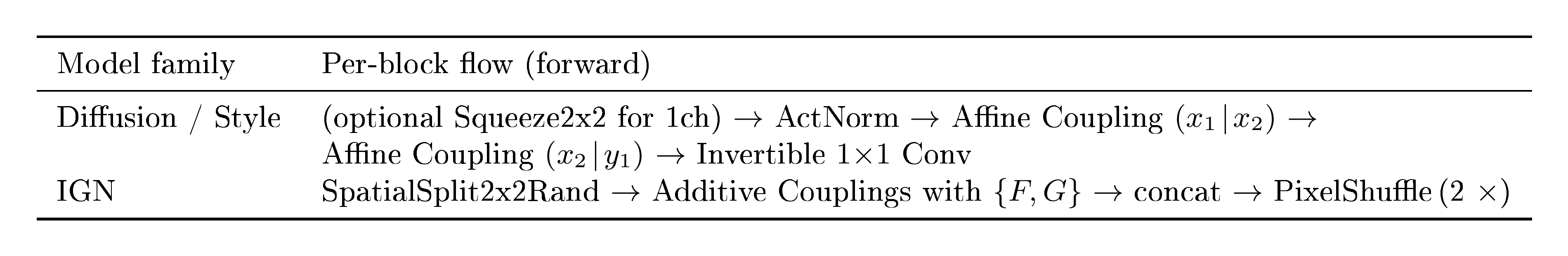
G.1 Backbones and Block Structure

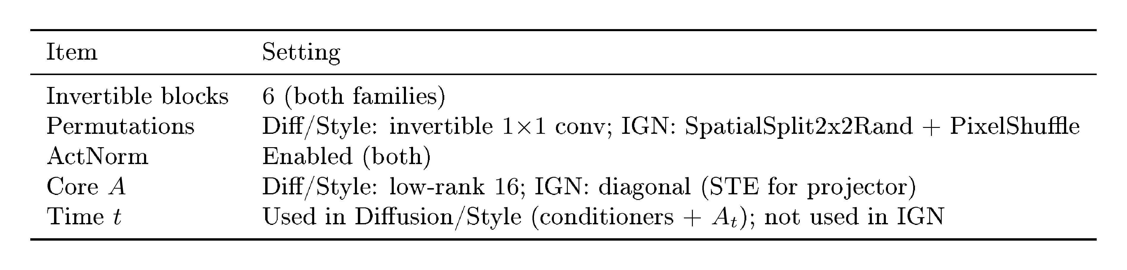
We use 6 invertible blocks in all models. The two architectures differ only in the internal block type:

::: {caption="Table 3: Block-level flow for the two architectures; repeated 6 times."}

:::

Notes.

• ActNorm: per-channel affine with data-dependent init on first batch.
• Affine coupling (Diffusion/Style): shift/log-scale predicted by a tiny U-Net conditioner; clamped $\log s$.
• Invertible $1{\times}1$ conv (Diffusion/Style): learned channel permutation/mixer (orthogonal init).
• SpatialSplit2x2Rand (IGN): deterministic $2{\times}2$ space partition into two streams; inverse merges.
• PixelShuffle / unshuffle (IGN): reversible $2{\times}$ spatial reindexing between blocks.
• We do not use InvTanhScaled.

The blocks:

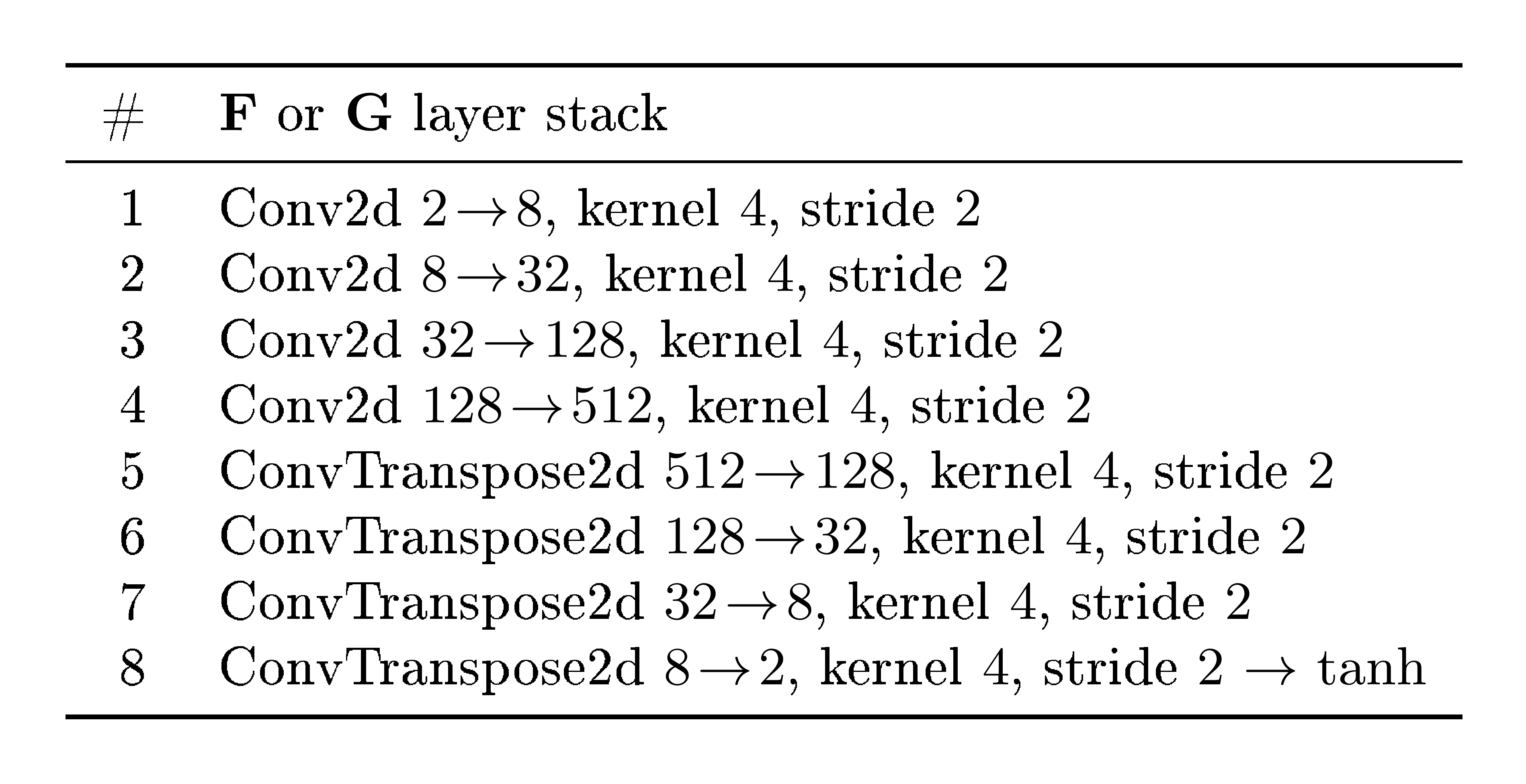
1. Diffusion/Style. We use a U-Net ([45]), adapting the implementation of [46]. We modify only two hyperparameters: model_channels $=16$ and channel_mult $=[1, 1]$.
2. IGN. We use bottleneck architecture, gradually downscaling to spatial size $1\times 1$ by stride 2 convolutions, and then using transposed convolutions back to original resolution. See table below for exact layers.

G.2 Time Path (Diffusion)

In diffusion/flow-matching models, the scalar $t$ is embedded and fed to: (i) the affine-coupling conditioners inside $g$, and (ii) the time-dependent core $A_t$ (low-rank MLP). Style and IGN models do not use $t$.

G.3 Cores $A$

• Diffusion: Two non-linear MLPs that produce two matrices for the low-rank parameterization $A = A_1 A_2$ with $\mathrm{rank}(A)=16$.
• Style. A kernel $4\times 4$ is produced by a non-linear hypernetwork $L({\text{style})} = A^{\text{style}}_{\mathrm{ker}}$, which we then apply to the image via a 2D convolution (PyTorch).
• IGN: diagonal $A$ (elementwise scale in latent); for idempotent IGN we threshold the diagonal with STE.

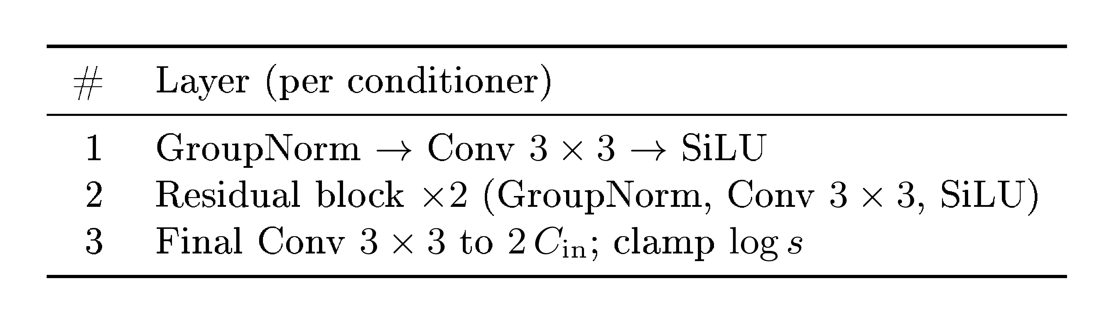
G.4 Conditioners

Diffusion / Style (Affine-coupling conditioners).

Each coupling uses a tiny U-Net that maps $C_{\text{in}}=C/2 \rightarrow 2, C_{\text{in}}$ (shift, $\log s$).

::: {caption="Table 4: Minimal U-Net-style conditioner used in affine couplings."}

:::

IGN (Additive-coupling CNNs).

Each coupling uses a plain CNN (no U-Net skip concatenations); forward is additive, inverse is exact.

::: {caption="Table 5: CNN used for $F$ and $G$ inside IGN additive couplings."}

:::

G.5 Losses (weights fixed)

IGN.

$ \lambda_{\text{rec}} = 1.0, \quad \lambda_{\text{sparse}} = 0.75, \quad \lambda_{\text{iso}} = 0.001. $

We use (i) reconstruction MSE, (ii) sparsity/rank on the diagonal of $A$, and (iii) a light isometry term on $g$.

Diffusion / Flow-Matching.

We use the main training loss described in the paper. For additional stability, we empirically found that adding the perceptual reconstruction terms $d(x_0, , g^{-1}(g(x_0)))$ and $d(x_1, , g^{-1}(g(x_1)))$ (with $d$ as LPIPS ([21])), together with the alignment term $\lVert A, g(x_0) - g(x_1)\rVert^2$, yields more stable training and higher-quality models. The primary loss in the paper also uses LPIPS as the distance metric. No explicit weighting between losses was required.

G.6 One-line Hyperparameter Summary

See Table.Table 6.

::: {caption="Table 6: Everything needed to reproduce the scaffolding."}

:::

H. Linearizer Universal Final Fit Theorem

Definition: Linearizer-realizable map

A function $F^* : \mathbb{R}^N \to \mathbb{R}^M$ is Linearizer-realizable if there exist a linear map $A^* : \mathbb{R}^N \to \mathbb{R}^M$ and diffeomorphisms $g_x^* : \mathbb{R}^N \to \mathbb{R}^N$ and $g_y^* : \mathbb{R}^M \to \mathbb{R}^M$ such that

$ F^*(x) ;=; (g_y^*)^{-1}!\bigl(A^*, g_x^*(x) \bigr) \qquad \text{for all } x \in \mathbb{R}^N. $

Fact 8: Diffeomorphism Extension on Finite Sets

Let $X = {x_1, \dots, x_n} \subset \mathbb{R}^N$ be a finite set of $n$ distinct points, and let $P = {p_1, \dots, p_n} \subset \mathbb{R}^N$ be any other finite set of $n$ distinct points.

There exists a global diffeomorphism $g^* : \mathbb{R}^N \to \mathbb{R}^N$ such that $g^*(x_i) = p_i$ for all $i = 1, \dots, n$.

Fact 9: INN Approximation, Teshima et al.\ 2020; informal

Let $K \subset \mathbb{R}^d$ be compact, and let $h : \mathbb{R}^d \to \mathbb{R}^d$ be a $C^1$ diffeomorphism.

For any $\eta > 0$, there exists an invertible neural network (INN) $H_\eta : \mathbb{R}^d \to \mathbb{R}^d$ such that $\sup_{z \in K} \lVert H_\eta(z) - h(z) \rVert < \eta$ and $\sup_{z \in h(K)} \lVert H_\eta^{-1}(z) - h^{-1}(z) \rVert < \eta$.

Lemma 10: Existence of a Realizable Fit

Let $X = {x_1, \dots, x_n} \subset \mathbb{R}^N$ be a finite set of distinct data points, and let $Y = {y_1, \dots, y_n} \subset \mathbb{R}^M$ be the corresponding target points.

There exists an ideal, Linearizer-realizable function $F^*$ that perfectly fits the data, i.e., $F^*(x_i) = y_i$ for all $i$.

Proof: Let $P = {p_1, \dots, p_n} \subset \mathbb{R}^N$ be a set of $n$ distinct latent points lying on the first coordinate axis, defined as $p_i = (i, 0, \dots, 0)^\top$.

We construct the linear map $A^*: \mathbb{R}^N \to \mathbb{R}^M$ to preserve the distinctness of these points by mapping the first axis of the domain to the first axis of the codomain. We distinguish two cases based on the dimensions:

• Case 1 ($M \le N$): We define $A^*$ as the projection onto the first $M$ coordinates. For any vector $v = (v_1, \dots, v_N)^\top \in \mathbb{R}^N$:

$ A^*(v) = (v_1, \dots, v_M)^\top \in \mathbb{R}^M. $

• Case 2 ($M > N$): We define $A^*$ as the canonical embedding (zero-padding) into the first $N$ coordinates. For any vector $v = (v_1, \dots, v_N)^\top \in \mathbb{R}^N$:

$ A^*(v) = (v_1, \dots, v_N, \underbrace{0, \dots, 0}_{M-N})^\top \in \mathbb{R}^M. $

In both cases, we define the target latent points as $Q = {q_1, \dots, q_n}$ where $q_i = A^* p_i$. Since the points $p_i$ differ in their first coordinate ($i$), and $A^*$ preserves the first coordinate in both cases (as $M, N \ge 1$), the resulting points $q_i$ are distinct in $\mathbb{R}^M$.

By Fact 8, there exists a global diffeomorphism $g_x^*: \mathbb{R}^N \to \mathbb{R}^N$ such that $g_x^*(x_i) = p_i$ for all $i$. Similarly, there exists a global diffeomorphism $g_y^*: \mathbb{R}^M \to \mathbb{R}^M$ such that $g_y^*(y_i) = q_i$ for all $i$.

We define the ideal Linearizer $F^*$ as:

$ F^*(x) := (g_y^*)^{-1}(A^* g_x^*(x)). $

Checking this function on the data points $x_i$:

$ F^*(x_i) = (g_y^*)^{-1}(A^* p_i) = (g_y^*)^{-1}(q_i) = y_i. $

Thus, a Linearizer-realizable function $F^*$ exists that perfectly fits the finite dataset.

Theorem 11: A Linearizer can fit any finite dataset

Let $X = {x_1, \dots, x_n} \subset \mathbb{R}^N$, $N\geq 2$, be a finite set and $F: X \to \mathbb{R}^M$ be the target function.

For every $\varepsilon > 0$, there exist invertible neural networks $G_x, G_y$ and a linear map $A$ such that the Linearizer $\hat{F}(x) := G_y^{-1}(A, G_x(x))$ achieves arbitrarily low error on the dataset:

$ \sup_{x \in X} \lVert \hat{F}(x) - F(x) \rVert < \varepsilon. $

Proof: By Lemma 10, there exists an ideal, Linearizer-realizable function $F^*(x) = (g_y^*)^{-1}(A^* g_x^*(x))$ such that $F(x) = F^*(x)$ for all $x \in X$. We need to prove that our INN-based architecture $\hat{F}$ can approximate $F^*$ on the compact set $X$.

Let $\varepsilon > 0$ be given. Set $A := A^*$. The proof follows the standard $\epsilon$- $\delta$ error decomposition.

$ \begin{aligned} \hat{F}(x) - F^*(x) &= G_y^{-1}!\bigl(A^* G_x(x)\bigr)

• (g_y^*)^{-1}!\bigl(A^* g_x^*(x)\bigr) \ &= \underbrace{ G_y^{-1}!\bigl(A^* G_x(x)\bigr)
• (g_y^*)^{-1}!\bigl(A^* G_x(x)\bigr) }_{(I)} ;+; \underbrace{ (g_y^*)^{-1}!\bigl(A^* G_x(x)\bigr)
• (g_y^*)^{-1}!\bigl(A^* g_x^*(x)\bigr) }_{(II)}. \end{aligned} $

The ideal diffeomorphisms $g_x^*$ and $(g_y^*)^{-1}$ are continuous and are being approximated on compact sets. By Fact 9, we can choose INNs $G_x$ and $G_y$ that are arbitrarily close to $g_x^*$ and $g_y^*$ (and their inverses) on these sets.

As both $(g_y^*)^{-1}$ and $A^*$ are continuous (and uniformly continuous on any compact set), we can make the norms of both terms (I) and (II) arbitrarily small by choosing sufficiently accurate INN approximations $G_x$ and $G_y$ (i.e., for a small enough $\delta$). We can thus choose $\delta$ such that the total error is

lt;\varepsilon$.

I. Additional Illustrations

References

[1] Strang, Gilbert (2022). Introduction to Linear Algebra. SIAM.

[2] Strogatz, Steven H. (2024). Nonlinear Dynamics and Chaos: With Applications to Physics, Biology, Chemistry, and Engineering. Chapman and Hall/CRC.

[3] Hornik et al. (1989). Multilayer Feedforward Networks are Universal Approximators. Neural Networks. 2(5). pp. 359–366.

[4] Mac Lane, Saunders and Birkhoff, Garrett (1999). Algebra. AMS Chelsea Publishing.

[5] Rezende, Danilo Jimenez and Mohamed, Shakir (2015). Variational Inference with Normalizing Flows. In Proceedings of the 32nd International Conference on Machine Learning (ICML). pp. 1530–1538.

[6] Dinh et al. (2015). NICE: Non-linear Independent Components Estimation. In Proceedings of the 2nd International Conference on Learning Representations (ICLR, Workshop Track).

[7] Dinh et al. (2017). Density Estimation using Real NVP. In Proceedings of the 5th International Conference on Learning Representations (ICLR).

[8] Lipman et al. (2023). Flow Matching for Generative Modeling. In International Conference on Learning Representations (ICLR).

[9] Song et al. (2021). Score-Based Generative Modeling through Stochastic Differential Equations. In International Conference on Learning Representations (ICLR).

[10] Ho et al. (2020). Denoising diffusion probabilistic models. Advances in neural information processing systems. 33. pp. 6840–6851.

[11] Gao et al. (2024). Diffusion meets flow matching: Two sides of the same coin. 2024. URL https://diffusionflow. github. io.

[12] Runge, Carl (1895). Über die numerische Auflösung von Differentialgleichungen. Mathematische Annalen. 46(2). pp. 167–178.

[13] Kutta, Wilhelm (1901). Beitrag zur näherungsweisen Integration totaler Differentialgleichungen. Teubner.

[14] LeCun et al. (1998). Gradient-based learning applied to document recognition. Proceedings of the IEEE. 86(11). pp. 2278–2324.

[15] Liu et al. (2015). Deep Learning Face Attributes in the Wild. In Proceedings of International Conference on Computer Vision (ICCV).

[16] Kingma, Diederik P. and Welling, Max (2014). Auto-Encoding Variational Bayes. In Proceedings of the 2nd International Conference on Learning Representations (ICLR).

[17] Dhariwal, Prafulla and Nichol, Alex (2021). Diffusion Models Beat GANs on Image Synthesis. In Advances in Neural Information Processing Systems (NeurIPS).

[18] Song et al. (2021). Denoising Diffusion Implicit Models. In International Conference on Learning Representations (ICLR).

[19] Huberman-Spiegelglas et al. (2024). Diffusion Inversion: A Universal Technique for Diffusion Editing and Interpolation. Transactions on Machine Learning Research (TMLR).

[20] Penrose, Roger (1955). A generalized inverse for matrices. Mathematical Proceedings of the Cambridge Philosophical Society. 51(3). pp. 406–413.

[21] Zhang et al. (2018). The unreasonable effectiveness of deep features as a perceptual metric. In Proceedings of the IEEE conference on computer vision and pattern recognition. pp. 586–595.

[22] Gatys et al. (2016). Image Style Transfer Using Convolutional Neural Networks. In Proceedings of the IEEE Conference on Computer Vision and Pattern Recognition (CVPR). pp. 2414–2423.

[23] Johnson et al. (2016). Perceptual Losses for Real-Time Style Transfer and Super-Resolution. In European Conference on Computer Vision (ECCV). pp. 694–711.

[24] Shocher et al. (2024). Idempotent Generative Network. In International Conference on Learning Representations (ICLR).

[25] Durasov et al. (2025). IT\textsuperscript3: Idempotent Test-Time Training. In Proceedings of the 42nd International Conference on Machine Learning (ICML).

[26] Jensen, Nikolaj Banke and Vicary, Jamie (2025). Enforcing Idempotency in Neural Networks. In Proceedings of the 42nd International Conference on Machine Learning (ICML).

[27] Bengio et al. (2013). Estimating or Propagating Gradients Through Stochastic Neurons. In Proceedings of the 2nd International Conference on Learning Representations (ICLR, Workshop Track).

[28] Wu et al. (2021). Autoformer: Decomposition transformers with auto-correlation for long-term series forecasting. Advances in neural information processing systems. 34. pp. 22419–22430.

[29] Nie, Y (2022). A Time Series is Worth 64Words: Long-term Forecasting with Transformers. arXiv preprint arXiv:2211.14730.

[30] Mezić, Igor (2005). Spectral Properties of Dynamical Systems, Model Reduction and Decompositions. Nonlinear Dynamics. 41. pp. 309–325.

[31] Schmid, Peter J. (2010). Dynamic Mode Decomposition of Numerical and Experimental Data. Journal of Fluid Mechanics. 656. pp. 5–28.

[32] Lusch et al. (2018). Deep Learning for Universal Linear Embeddings of Nonlinear Dynamics. Nature Communications. 9. pp. 4950.

[33] Mardt et al. (2018). VAMPnets for Deep Learning of Molecular Kinetics. Nature Communications. 9. pp. 5.

[34] Jacot et al. (2018). Neural Tangent Kernel: Convergence and Generalization in Neural Networks. In Advances in Neural Information Processing Systems (NeurIPS).

[35] Salimans, Tim and Ho, Jonathan (2022). Progressive Distillation for Fast Sampling of Diffusion Models. In Advances in Neural Information Processing Systems (NeurIPS).

[36] Song et al. (2023). Consistency Models. In Proceedings of the 40th International Conference on Machine Learning (ICML).

[37] Berman et al. (2025). One-Step Offline Distillation of Diffusion-based Models via Koopman Modeling. In Proceedings of the 42nd International Conference on Machine Learning (ICML).

[38] Kingma, Diederik P. and Dhariwal, Prafulla (2018). Glow: Generative Flow with Invertible 1x1 Convolutions. In Advances in Neural Information Processing Systems (NeurIPS).

[39] Quessard et al. (2020). Learning Group Structure and Disentangled Representations of Dynamical Environments. In Advances in Neural Information Processing Systems (NeurIPS).

[40] Psenka et al. (2024). Representation Learning via Manifold Flattening and Reconstruction. Journal of Machine Learning Research.

[41] Bône et al. (2019). Learning Low-Dimensional Representations of Shape Data Sets with Diffeomorphic Autoencoders. In Information Processing in Medical Imaging (IPMI). pp. 195–207.

[42] Saxe et al. (2014). Exact Solutions to the Nonlinear Dynamics of Learning in Deep Linear Neural Networks. In International Conference on Learning Representations (ICLR).

[43] Arora et al. (2018). On the Optimization of Deep Networks: Implicit Acceleration by Overparameterization. In Proceedings of the 35th International Conference on Machine Learning (ICML). pp. 244–253.

[44] Cohen et al. (2016). On the Expressive Power of Deep Learning: A Tensor Analysis. In Proceedings of the 29th Annual Conference on Learning Theory (COLT).

[45] Ronneberger et al. (2015). U-net: Convolutional networks for biomedical image segmentation. In International Conference on Medical image computing and computer-assisted intervention. pp. 234–241.

[46] Karras et al. (2022). Elucidating the design space of diffusion-based generative models. Advances in neural information processing systems. 35. pp. 26565–26577.