Dueling Network Architectures for Deep Reinforcement Learning

Ziyu Wang
Tom Schaul
Matteo Hessel
Hado van Hasselt
Marc Lanctot
Nando de Freitas
Google DeepMind, London, UK

Abstract

In recent years there have been many successes of using deep representations in reinforcement learning. Still, many of these applications use conventional architectures, such as convolutional networks, LSTMs, or auto-encoders. In this paper, we present a new neural network architecture for model-free reinforcement learning. Our dueling network represents two separate estimators: one for the state value function and one for the state-dependent action advantage function. The main benefit of this factoring is to generalize learning across actions without imposing any change to the underlying reinforcement learning algorithm. Our results show that this architecture leads to better policy evaluation in the presence of many similar-valued actions. Moreover, the dueling architecture enables our RL agent to outperform the state-of-the-art on the Atari 2600 domain.

Executive Summary: The document introduces a new neural network design for model-free reinforcement learning called the dueling architecture. Standard deep networks estimate the value of each possible action in every state. The new design instead splits estimation into two streams that share early layers: one stream learns how good a state is overall, while the other learns the relative benefit of each action. These streams combine at the output to produce action values that existing algorithms can use without modification.

The work addresses a practical limitation. In many control problems, especially those with large or redundant action sets, learning a separate value for every action wastes capacity on states where actions make little difference. The authors therefore set out to test whether an architecture that factors state value and action advantage would improve learning speed and final performance while remaining compatible with current reinforcement-learning methods.

They evaluated the approach in two stages. First, they ran controlled policy-evaluation experiments in a simple corridor environment that allowed exact computation of true values. They then trained agents on all 57 games in the Atari 2600 benchmark using the Double DQN algorithm, both with and without prioritized experience replay, and compared results against single-stream baselines of similar capacity. Training used the same hyper-parameters and pixel-plus-score inputs as prior work.

The dueling architecture produced three main results. In the corridor task, it converged faster once the number of actions rose from five to ten or twenty. Across the Atari suite it outperformed the single-stream baseline on roughly three-quarters of the games and reached higher scores on more than 80 percent of them. When combined with prioritized replay and gradient clipping, the resulting agent achieved a new state-of-the-art mean score of 592 percent of human performance (median 172 percent) under the standard 30-no-op evaluation protocol.

These gains matter because they require no change to the underlying learning algorithm. The architecture simply allocates more learning effort to estimating state values, which temporal-difference methods rely on heavily. The improvement grows with action-space size and complements other recent advances such as prioritized replay. As a result, agents reach stronger policies with the same amount of experience.

The authors recommend that practitioners adopt the dueling design as a drop-in replacement for conventional Q-networks, particularly in domains with many actions. They also suggest testing further combinations with other algorithmic improvements. The main limitations are that all results come from the Atari domain and that a few games remain far below human performance; broader validation on additional tasks would increase confidence. Overall, the evidence for Atari is strong because the evaluation covered every game with consistent protocols and multiple random seeds.

1. Introduction

Section Summary: Recent advances in deep reinforcement learning have largely relied on standard neural networks paired with improved training algorithms. This paper instead introduces a dueling network architecture that splits the estimation of how good a situation is overall from how much each possible action adds or subtracts from that value, then recombines the two streams to produce action values. By learning these quantities separately, the network can more efficiently recognize valuable states even when many actions have little effect, yielding faster learning and stronger results on Atari games.

Over the past years, deep learning has contributed to dramatic advances in scalability and performance of machine learning [1]. One exciting application is the sequential decision-making setting of reinforcement learning (RL) and control. Notable examples include deep Q-learning [2], deep visuomotor policies [3], attention with recurrent networks [4], and model predictive control with embeddings [5]. Other recent successes include massively parallel frameworks [6] and expert move prediction in the game of Go [7], which produced policies matching those of Monte Carlo tree search programs, and squarely beaten a professional player when combined with search [8].

In spite of this, most of the approaches for RL use standard neural networks, such as convolutional networks, MLPs, LSTMs and autoencoders. The focus in these recent advances has been on designing improved control and RL algorithms, or simply on incorporating existing neural network architectures into RL methods. Here, we take an alternative but complementary approach of focusing primarily on innovating a neural network architecture that is better suited for model-free RL. This approach has the benefit that the new network can be easily combined with existing and future algorithms for RL. That is, this paper advances a new network (Figure 1), but uses already published algorithms.

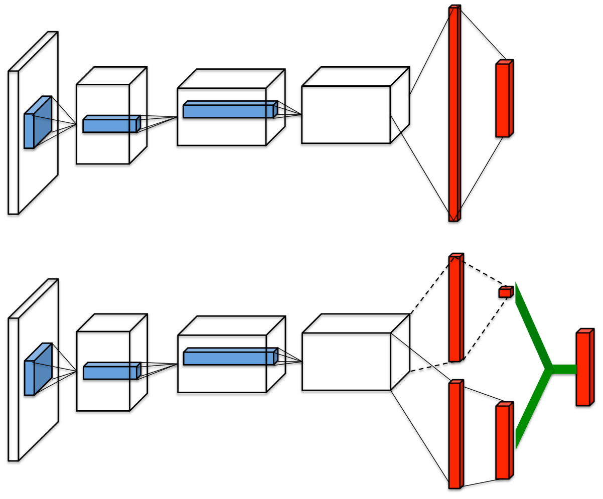
The proposed network architecture, which we name the dueling architecture, explicitly separates the representation of state values and (state-dependent) action advantages. The dueling architecture consists of two streams that represent the value and advantage functions, while sharing a common convolutional feature learning module. The two streams are combined via a special aggregating layer to produce an estimate of the state-action value function $Q$ as shown in Figure 1. This dueling network should be understood as a single $Q$ network with two streams that replaces the popular single-stream $Q$ network in existing algorithms such as Deep Q-Networks (DQN; [2]). The dueling network automatically produces separate estimates of the state value function and advantage function, without any extra supervision.

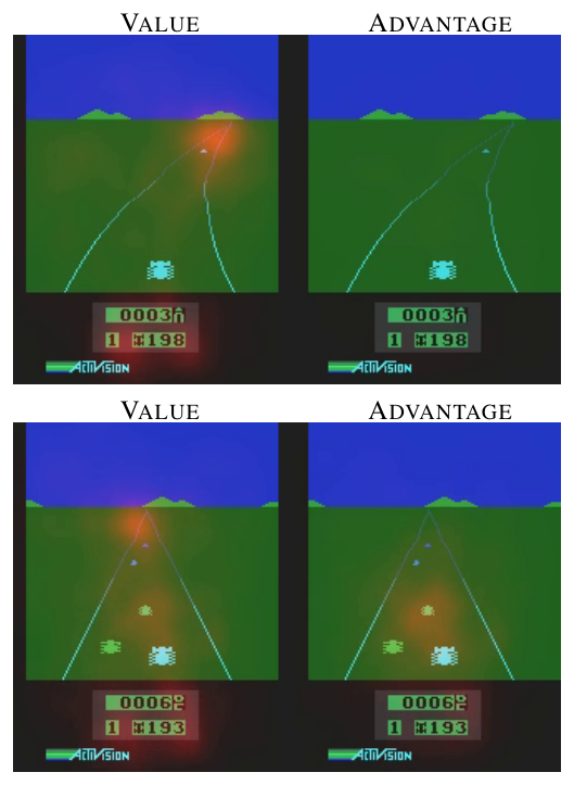
Intuitively, the dueling architecture can learn which states are (or are not) valuable, without having to learn the effect of each action for each state. This is particularly useful in states where its actions do not affect the environment in any relevant way. To illustrate this, consider the saliency maps shown in Figure 2^1. These maps were generated by computing the Jacobians of the trained value and advantage streams with respect to the input video, following the method proposed by [9]. (The experimental section describes this methodology in more detail.) The figure shows the value and advantage saliency maps for two different time steps. In one time step (leftmost pair of images), we see that the value network stream pays attention to the road and in particular to the horizon, where new cars appear. It also pays attention to the score. The advantage stream on the other hand does not pay much attention to the visual input because its action choice is practically irrelevant when there are no cars in front. However, in the second time step (rightmost pair of images) the advantage stream pays attention as there is a car immediately in front, making its choice of action very relevant.

In the experiments, we demonstrate that the dueling architecture can more quickly identify the correct action during policy evaluation as redundant or similar actions are added to the learning problem.

We also evaluate the gains brought in by the dueling architecture on the challenging Atari 2600 testbed. Here, an RL agent with the same structure and hyper-parameters must be able to play 57 different games by observing image pixels and game scores only. The results illustrate vast improvements over the single-stream baselines of [2] and [10]. The combination of prioritized replay ([11]) with the proposed dueling network results in the new state-of-the-art for this popular domain.

1.1 Related Work

The notion of maintaining separate value and advantage functions goes back to [12]. In Baird's original advantage updating algorithm, the shared Bellman residual update equation is decomposed into two updates: one for a state value function, and one for its associated advantage function. Advantage updating was shown to converge faster than Q-learning in simple continuous time domains in [13]. Its successor, the advantage learning algorithm, represents only a single advantage function [14].

The dueling architecture represents both the value $V(s)$ and advantage $A(s, a)$ functions with a single deep model whose output combines the two to produce a state-action value $Q(s, a)$. Unlike in advantage updating, the representation and algorithm are decoupled by construction. Consequently, the dueling architecture can be used in combination with a myriad of model free RL algorithms.

There is a long history of advantage functions in policy gradients, starting with [15]. As a recent example of this line of work, [16] estimate advantage values online to reduce the variance of policy gradient algorithms.

There have been several attempts at playing Atari with deep reinforcement learning, including [2, 17, 18, 6, 10, 19] and [11]. The results of [11] are the current published state-of-the-art.

2. Background

Section Summary: In sequential decision-making tasks such as Atari games, an agent observes video-frame states, selects actions from a discrete set, and receives rewards while seeking to maximize the expected discounted sum of future rewards. Core quantities include the Q-function for state-action values, the state value function, and the advantage function that highlights relative action quality, all satisfying a recursive Bellman equation for optimality. These are approximated by deep Q-networks trained via gradient descent on sampled experiences, stabilized by a separate target network, experience replay, double Q-learning to curb overoptimism, and prioritized sampling of high-error transitions.

We consider a sequential decision making setup, in which an agent interacts with an environment $\mathcal{E}$ over discrete time steps, see [20] for an introduction. In the Atari domain, for example, the agent perceives a video $s_t$ consisting of $M$ image frames: $s_t =(x_{t-M+1}, \ldots, x_t) \in \mathcal{S}$ at time step $t$. The agent then chooses an action from a discrete set $a_t \in \mathcal{A} = {1, \ldots, |\mathcal{A}|} $ and observes a reward signal $r_t$ produced by the game emulator.

The agent seeks maximize the expected discounted return, where we define the discounted return as $R_t = \sum_{\tau=t}^{\infty} \gamma^{\tau-t} r_{\tau}$. In this formulation, $\gamma \in [0, 1]$ is a discount factor that trades-off the importance of immediate and future rewards.

For an agent behaving according to a stochastic policy $\pi$, the values of the state-action pair $(s, a)$ and the state $s$ are defined as follows

$ \begin{aligned} Q^{\pi}(s, a) &=& \mathbb{E}\left[{\left. R_t \right| s_t = s, a_t = a, \pi} \right], ~\text{ and } \nonumber \ V^{\pi}(s) &=& \mathbb{E}_{{a \sim \pi(s)}} \left[{Q^{\pi}(s, a)} \right]. \end{aligned} $

The preceding state-action value function ($Q$ function for short) can be computed recursively with dynamic programming:

$ Q^{\pi}(s, a) = \mathbb{E}{{s'}} \left[{r + \gamma \mathbb{E}{{a'\sim\pi(s')}} \left[{Q^{\pi}(s', a')} \right]|s, a, \pi} \right]. $

We define the optimal $Q^{}(s, a) = \max_{\pi} Q^{\pi}(s, a).$ Under the deterministic policy $a = \operatorname{arg, max}_{a' \in \mathcal{A}} Q^{}(s, a')$, it follows that $V^{}(s) = \max_{a} Q^{}(s, a).$ From this, it also follows that the optimal $Q$ function satisfies the Bellman equation:

$ Q^{}(s, a) = \mathbb{E}{s'} \left[r + \gamma \max{a' } Q^{}(s', a') | s, a \right].\tag{1} $

We define another important quantity, the advantage function, relating the value and $Q$ functions:

$ A^{\pi}(s, a) = Q^{\pi}(s, a) - V^{\pi}(s).\tag{2} $

Note that $\mathbb{E}_{{a \sim \pi(s)}} \left[{A^{\pi}(s, a)} \right] = 0$. Intuitively, the value function $V$ measures the how good it is to be in a particular state $s$. The $Q$ function, however, measures the the value of choosing a particular action when in this state. The advantage function subtracts the value of the state from the Q function to obtain a relative measure of the importance of each action.

2.1 Deep Q-networks

The value functions as described in the preceding section are high dimensional objects. To approximate them, we can use a deep $Q$-network: $Q(s, a;\theta)$ with parameters $\theta$. To estimate this network, we optimize the following sequence of loss functions at iteration $i$:

$ L_i(\theta_i) = \mathbb{E}{s, a, r, s'} \left[\left(y_i^{DQN} - Q(s, a; \theta{i}) \right)^{2} \right],\tag{3} $

with

$ y_i^{DQN} = r + \gamma \max_{a'} Q(s', a';\theta^{-}),\tag{4} $

where $\theta^{-}$ represents the parameters of a fixed and separate target network. We could attempt to use standard $Q$-learning to learn the parameters of the network $Q(s, a; \theta)$ online. However, this estimator performs poorly in practice. A key innovation in ([2]) was to freeze the parameters of the target network $Q(s', a';\theta^{-})$ for a fixed number of iterations while updating the online network $Q(s, a; \theta_{i})$ by gradient descent. (This greatly improves the stability of the algorithm.) The specific gradient update is

$ \begin{aligned} &\nabla_{\theta_i} L_i(\theta_i) = \displaystyle{\mathbb{E}{s, a, r, s'}} \Big[\left(y_i^{DQN} - Q(s, a; \theta{i}) \right) \nabla_{\theta_i} Q(s, a; \theta_{i}) \Big] \nonumber& \end{aligned} $

This approach is model free in the sense that the states and rewards are produced by the environment. It is also off-policy because these states and rewards are obtained with a behavior policy (epsilon greedy in DQN) different from the online policy that is being learned.

Another key ingredient behind the success of DQN is experience replay ([21, 2]). During learning, the agent accumulates a dataset $\mathcal{D}t ={e_1, e_2, \ldots, e_t}$ of experiences $e_t=(s_t, a_t, r_t, s{t+1})$ from many episodes. When training the $Q$-network, instead only using the current experience as prescribed by standard temporal-difference learning, the network is trained by sampling mini-batches of experiences from $\mathcal{D}$ uniformly at random. The sequence of losses thus takes the form

$ L_i(\theta_i) = \mathbb{E}{(s, a, r, s')\sim \mathcal{U}(\mathcal{D}) } \left[\left(y_i^{DQN} - Q(s, a; \theta{i}) \right)^{2} \right]. \nonumber\tag{5} $

Experience replay increases data efficiency through re-use of experience samples in multiple updates and, importantly, it reduces variance as uniform sampling from the replay buffer reduces the correlation among the samples used in the update.

2.2 Double Deep Q-networks

The previous section described the main components of DQN as presented in ([2]). In this paper, we use the improved Double DQN (DDQN) learning algorithm of [10]. In Q-learning and DQN, the $\max$ operator uses the same values to both select and evaluate an action. This can therefore lead to overoptimistic value estimates ([22]). To mitigate this problem, DDQN uses the following target:

$ y_i^{DDQN} = r + \gamma Q(s', \operatorname{arg, max}_{a'} Q(s', a';\theta_i) ;\theta^{-}).\tag{6} $

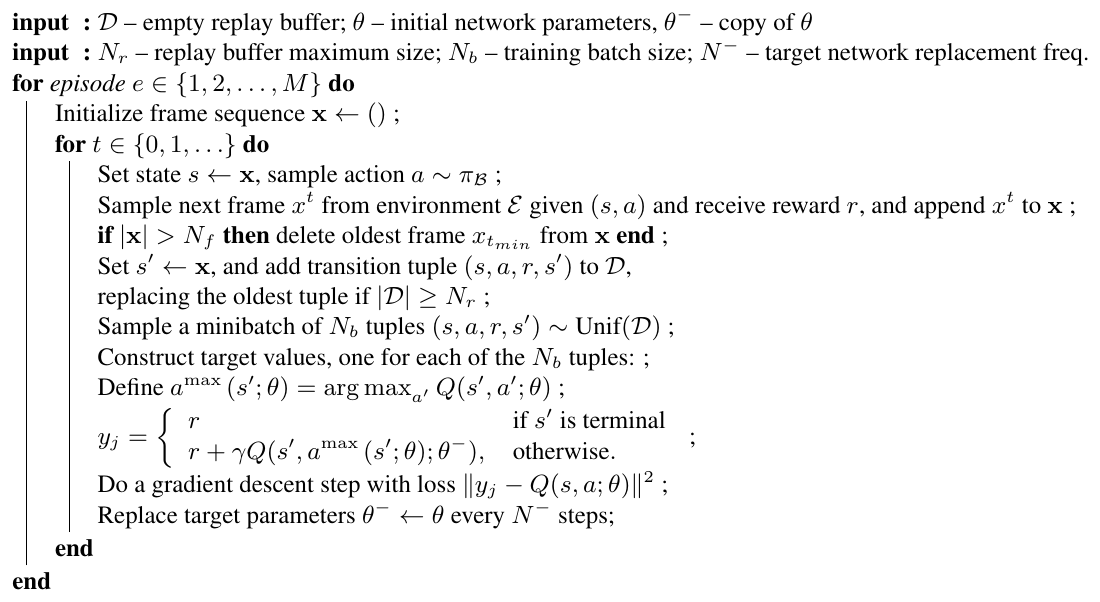
DDQN is the same as for DQN (see [2]), but with the target $y_i^{DQN}$ replaced by $ y_i^{DDQN}$. The pseudo-code for DDQN is presented in Appendix A.

2.3 Prioritized Replay

A recent innovation in prioritized experience replay ([11]) built on top of DDQN and further improved the state-of-the-art. Their key idea was to increase the replay probability of experience tuples that have a high expected learning progress (as measured via the proxy of absolute TD-error). This led to both faster learning and to better final policy quality across most games of the Atari benchmark suite, as compared to uniform experience replay.

To strengthen the claim that our dueling architecture is complementary to algorithmic innovations, we show that it improves performance for both the uniform and the prioritized replay baselines (for which we picked the easier to implement rank-based variant), with the resulting prioritized dueling variant holding the new state-of-the-art.

3. The Dueling Network Architecture

Section Summary: The dueling network modifies a standard deep Q-network by splitting its upper layers into two separate streams after shared convolutional processing: one stream estimates the overall value of a given state, while the other estimates the relative advantage of each possible action in that state. These two estimates are then combined through a specialized aggregation step—typically by subtracting the average advantage—to produce the final Q-values for each action, ensuring the decomposition remains stable and identifiable during training. Because the architecture still outputs ordinary Q-values, it can be trained end-to-end with existing algorithms such as DDQN while allowing the network to focus learning effort on state values that matter even when action choice is irrelevant.

The key insight behind our new architecture, as illustrated in Figure 2, is that for many states, it is unnecessary to estimate the value of each action choice. For example, in the Enduro game setting, knowing whether to move left or right only matters when a collision is eminent. In some states, it is of paramount importance to know which action to take, but in many other states the choice of action has no repercussion on what happens. For bootstrapping based algorithms, however, the estimation of state values is of great importance for every state.

To bring this insight to fruition, we design a single $Q$-network architecture, as illustrated in Figure 1, which we refer to as the dueling network. The lower layers of the dueling network are convolutional as in the original DQNs [2]. However, instead of following the convolutional layers with a single sequence of fully connected layers, we instead use two sequences (or streams) of fully connected layers. The streams are constructed such that they have they have the capability of providing separate estimates of the value and advantage functions. Finally, the two streams are combined to produce a single output $Q$ function. As in [2], the output of the network is a set of $Q$ values, one for each action.

Since the output of the dueling network is a $Q$ function, it can be trained with the many existing algorithms, such as DDQN and SARSA. In addition, it can take advantage of any improvements to these algorithms, including better replay memories, better exploration policies, intrinsic motivation, and so on.

The module that combines the two streams of fully-connected layers to output a $Q$ estimate requires very thoughtful design.

From the expressions for advantage $Q^{\pi}(s, a) = V^{\pi}(s) + A^{\pi}(s, a)$ and state-value $V^{\pi}(s) = \mathbb{E}{{a \sim \pi(s)}} \left[{Q^{\pi}(s, a)} \right]$, it follows that $\mathbb{E}{{a \sim \pi(s)}} \left[{A^{\pi}(s, a)} \right] = 0$. Moreover, for a deterministic policy, $a^* = \operatorname{arg, max}_{a' \in \mathcal{A}} Q(s, a')$, it follows that $Q(s, a^*) = V(s)$ and hence $A(s, a^*)=0$.

Let us consider the dueling network shown in Figure 1, where we make one stream of fully-connected layers output a scalar ${V}(s;\theta, \beta)$, and the other stream output an $|\mathcal{A}|$-dimensional vector ${A}(s, a;\theta, \alpha)$. Here, $\theta$ denotes the parameters of the convolutional layers, while $\alpha$ and $\beta$ are the parameters of the two streams of fully-connected layers.

Using the definition of advantage, we might be tempted to construct the aggregating module as follows:

$ Q(s, a;\theta, \alpha, \beta) = V(s;\theta, \beta) + A(s, a;\theta, \alpha),\tag{7} $

Note that this expression applies to all $(s, a)$ instances; that is, to express equation (7) in matrix form we need to replicate the scalar, ${V}(s;\theta, \beta)$, $|\mathcal{A}|$ times.

However, we need to keep in mind that $Q(s, a;\theta, \alpha, \beta)$ is only a parameterized estimate of the true $Q$-function. Moreover, it would be wrong to conclude that ${V}(s;\theta, \beta)$ is a good estimator of the state-value function, or likewise that ${A}(s, a;\theta, \alpha)$ provides a reasonable estimate of the advantage function.

Equation (7) is unidentifiable in the sense that given $Q$ we cannot recover ${V}$ and ${A}$ uniquely. To see this, add a constant to ${V}(s;\theta, \beta)$ and subtract the same constant from ${A}(s, a;\theta, \alpha)$. This constant cancels out resulting in the same $Q$ value. This lack of identifiability is mirrored by poor practical performance when this equation is used directly.

To address this issue of identifiability, we can force the advantage function estimator to have zero advantage at the chosen action. That is, we let the last module of the network implement the forward mapping

$ \begin{split} Q(s, a;\theta, \alpha, \beta) = V(s;\theta, \beta)~+\ \left(A(s, a;\theta, \alpha) - \max_{a' \in |\mathcal{A}|} A(s, a' ;\theta, \alpha) \right). \end{split}\tag{8} $

Now, for $a^* = \operatorname{arg, max}{a' \in \mathcal{A}} Q(s, a';\theta, \alpha, \beta) = \operatorname{arg, max}{a' \in \mathcal{A}} A(s, a';\theta, \alpha)$, we obtain $Q(s, a^*;\theta, \alpha, \beta) = V(s;\theta, \beta)$. Hence, the stream ${V}(s;\theta, \beta)$ provides an estimate of the value function, while the other stream produces an estimate of the advantage function.

An alternative module replaces the max operator with an average:

$ \begin{split} Q(s, a;\theta, \alpha, \beta) = V(s;\theta, \beta)~+\ \left(A(s, a;\theta, \alpha) - \frac{1}{|\mathcal{A}|} \sum_{a'} A(s, a' ;\theta, \alpha) \right). \end{split}\tag{9} $

On the one hand this loses the original semantics of $V$ and $A$ because they are now off-target by a constant, but on the other hand it increases the stability of the optimization: with Equation (9) the advantages only need to change as fast as the mean, instead of having to compensate any change to the optimal action's advantage in Equation (8). We also experimented with a softmax version of equation (8), but found it to deliver similar results to the simpler module of equation (9). Hence, all the experiments reported in this paper use the module of equation (9).

Note that while subtracting the mean in equation (9) helps with identifiability, it does not change the relative rank of the ${A}$ (and hence $Q$) values, preserving any greedy or $\epsilon$-greedy policy based on $Q$ values from equation (7). When acting, it suffices to evaluate the advantage stream to make decisions.

It is important to note that equation (9) is viewed and implemented as part of the network and not as a separate algorithmic step. Training of the dueling architectures, as with standard $Q$ networks (e.g. the deep $Q$-network of [2]), requires only back-propagation. The estimates ${V}(s;\theta, \beta)$ and ${A}(s, a;\theta, \alpha)$ are computed automatically without any extra supervision or algorithmic modifications.

As the dueling architecture shares the same input-output interface with standard $Q$ networks, we can recycle all learning algorithms with $Q$ networks (e.g., DDQN and SARSA) to train the dueling architecture.

4. Experiments

Section Summary: The experiments first evaluate the dueling architecture on a straightforward policy-learning task inside a simple corridor environment with varying numbers of actions. Results show that separating value and advantage streams allows faster, more stable learning than a conventional single-stream network, since the value estimate can be shared across similar actions. The same architecture is then scaled up and tested on 57 Atari games using raw pixel inputs and the DDQN algorithm, where it delivers consistent gains over standard Q-networks.

We now show the practical performance of the dueling network. We start with a simple policy evaluation task and then show larger scale results for learning policies for general Atari game-playing.

4.1 Policy evaluation

We start by measuring the performance of the dueling architecture on a policy evaluation task. We choose this particular task because it is very useful for evaluating network architectures, as it is devoid of confounding factors such as the choice of exploration strategy, and the interaction between policy improvement and policy evaluation.

In this experiment, we employ temporal difference learning (without eligibility traces, i.e., $\lambda = 0$) to learn $Q$ values. More specifically, given a behavior policy $\pi$, we seek to estimate the state-action value $Q^{\pi}(\cdot, \cdot)$ by optimizing the sequence of costs of equation (3), with target

$ y_i = r + \gamma \mathbb{E}_{a' \sim \pi(s')}\left[Q(s', a';\theta_i) \right]. $

The above update rule is the same as that of Expected SARSA [23]. We, however, do not modify the behavior policy as in Expected SARSA.

To evaluate the learned $Q$ values, we choose a simple environment where the exact $Q^\pi(s, a)$ values can be computed separately for all $(s, a) \in \cal{S} \times \cal{A}$. This environment, which we call the corridor is composed of three connected corridors. A schematic drawing of the corridor environment is shown in Figure 3, The agent starts from the bottom left corner of the environment and must move to the top right to get the largest reward. A total of $5$ actions are available: go up, down, left, right and no-op. We also have the freedom of adding an arbitrary number of no-op actions. In our setup, the two vertical sections both have 10 states while the horizontal section has 50.

We use an $\epsilon$-greedy policy as the behavior policy $\pi$, which chooses a random action with probability $\epsilon$ or an action according to the optimal $Q$ function $\operatorname{arg, max}_{a \in \cal{A}}Q^*(s, a)$ with probability $1-\epsilon$. In our experiments, $\epsilon$ is chosen to be $0.001$.

We compare a single-stream $Q$ architecture with the dueling architecture on three variants of the corridor environment with 5, 10 and 20 actions respectively. The 10 and 20 action variants are formed by adding no-ops to the original environment. We measure performance by Squared Error (SE) against the true state values: $\sum_{s \in \mathcal{S}, a \in \mathcal{A}} (Q(s, a;\theta) - Q^{\pi}(s, a))^2$. The single-stream architecture is a three layer MLP with $50$ units on each hidden layer. The dueling architecture is also composed of three layers. After the first hidden layer of 50 units, however, the network branches off into two streams each of them a two layer MLP with 25 hidden units. The results of the comparison are summarized in Figure 3.

The results show that with $5$ actions, both architectures converge at about the same speed. However, when we increase the number of actions, the dueling architecture performs better than the traditional $Q$-network. In the dueling network, the stream ${V}(s;\theta, \beta)$ learns a general value that is shared across many similar actions at $s$, hence leading to faster convergence. This is a very promising result because many control tasks with large action spaces have this property, and consequently we should expect that the dueling network will often lead to much faster convergence than a traditional single stream network. In the following section, we will indeed see that the dueling network results in substantial gains in performance in a wide-range of Atari games.

4.2 General Atari Game-Playing

We perform a comprehensive evaluation of our proposed method on the Arcade Learning Environment [24], which is composed of 57 Atari games. The challenge is to deploy a single algorithm and architecture, with a fixed set of hyper-parameters, to learn to play all the games given only raw pixel observations and game rewards. This environment is very demanding because it is both comprised of a large number of highly diverse games and the observations are high-dimensional.

We follow closely the setup of [10] and compare to their results using single-stream $Q$-networks. We train the dueling network with the DDQN algorithm as presented in Appendix A. At the end of this section, we incorporate prioritized experience replay [11].

Our network architecture has the same low-level convolutional structure of DQN [2, 10]. There are 3 convolutional layers followed by 2 fully-connected layers. The first convolutional layer has 32 $8 \times 8$ filters with stride 4, the second 64 $4 \times 4$ filters with stride 2, and the third and final convolutional layer consists 64 $3 \times 3$ filters with stride 1. As shown in Figure 1, the dueling network splits into two streams of fully connected layers. The value and advantage streams both have a fully-connected layer with 512 units. The final hidden layers of the value and advantage streams are both fully-connected with the value stream having one output and the advantage as many outputs as there are valid actions[^2]. We combine the value and advantage streams using the module described by Equation (9). Rectifier non-linearities [25] are inserted between all adjacent layers.

[^2]: The number of actions ranges between 3-18 actions in the ALE environment.

We adopt the optimizers and hyper-parameters of [10], with the exception of the learning rate which we chose to be slightly lower (we do not do this for double DQN as it can deteriorate its performance). Since both the advantage and the value stream propagate gradients to the last convolutional layer in the backward pass, we rescale the combined gradient entering the last convolutional layer by $1/\sqrt{2}$. This simple heuristic mildly increases stability. In addition, we clip the gradients to have their norm less than or equal to 10. This clipping is not standard practice in deep RL, but common in recurrent network training [26].

To isolate the contributions of the dueling architecture, we re-train DDQN with a single stream network using exactly the same procedure as described above. Specifically, we apply gradient clipping, and use $1024$ hidden units for the first fully-connected layer of the network so that both architectures (dueling and single) have roughly the same number of parameters. We refer to this re-trained model as Single Clip, while the original trained model of [10] is referred to as Single.

As in [10], we start the game with up to 30 no-op actions to provide random starting positions for the agent. To evaluate our approach, we measure improvement in percentage (positive or negative) in score over the better of human and baseline agent scores:

$ {\frac{\text{Score}{\text{Agent}} - \text{Score}{\text{Baseline}}} \max{ \text{Score}{\text{Human}}, \text{Score}{\text{Baseline}} } - \text{Score}_{\text{Random}} }\tag{10} $

We took the maximum over human and baseline agent scores as it prevents insignificant changes to appear as large improvements when neither the agent in question nor the baseline are doing well. For example, an agent that achieves 2% human performance should not be interpreted as two times better when the baseline agent achieves 1% human performance. We also chose not to measure performance in terms of percentage of human performance alone because a tiny difference relative to the baseline on some games can translate into hundreds of percent in human performance difference.

The results for the wide suite of 57 games are summarized in Table 1. Detailed results are presented in the Appendix.

Using this 30 no-ops performance measure, it is clear that the dueling network (Duel Clip) does substantially better than the Single Clip network of similar capacity. It also does considerably better than the baseline (Single) of [10]. For comparison we also show results for the deep $Q$-network of [2], referred to as Nature DQN.

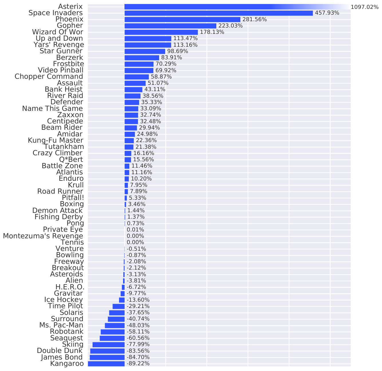
Figure 4 shows the improvement of the dueling network over the baseline Single network of [10]. Again, we seen that the improvements are often very dramatic.

As shown in Table 1, Single Clip performs better than Single. We verified that this gain was mostly brought in by gradient clipping. For this reason, we incorporate gradient clipping in all the new approaches.

\begin{tabular}{l|rr|rr}
\multicolumn{1}{c}{\bf } &\multicolumn{2}{c}{\bf 30 no-ops} &\multicolumn{2}{c}{\bf Human Starts} \\
 \hline
\multicolumn{1}{c}{\bf } &\multicolumn{1}{r}{\bf Mean} &\multicolumn{1}{r}{\bf Median}&\multicolumn{1}{r}{\bf Mean} &\multicolumn{1}{r}{\bf Median}
\\ \hline 
Prior. Duel Clip & {\bf 591.9}\% & {\bf 172.1}\% & {\bf 567.0}\% & {\bf 115.3}\% \\
Prior. Single& 434.6\% & 123.7\% & 386.7\% & 112.9\% \\
\hline
Duel Clip & {\bf 373.1}\% & {\bf 151.5}\% & {\bf 343.8}\% & {\bf 117.1}\% \\
Single Clip & 341.2\% & 132.6\% & 302.8\% & 114.1\% \\
Single & 307.3\% & 117.8\% & 332.9\% & 110.9\% \\
\hline
Nature DQN & 227.9\% & 79.1\% & 219.6\% & 68.5\% 
\end{tabular}

Duel Clip does better than Single Clip on 75.4% of the games (43 out of 57). It also achieves higher scores compared to the Single baseline on 80.7% ($46$ out of $57$) of the games. Of all the games with $18$ actions, Duel Clip is better $86.6$ % of the time (26 out of 30). This is consistent with the findings of the previous section. Overall, our agent (Duel Clip) achieves human level performance on 42 out of 57 games. Raw scores for all the games, as well as measurements in human performance percentage, are presented in the Appendix.

Robustness to human starts. One shortcoming of the 30 no-ops metric is that an agent does not necessarily have to generalize well to play the Atari games. Due to the deterministic nature of the Atari environment, from an unique starting point, an agent could learn to achieve good performance by simply remembering sequences of actions.

To obtain a more robust measure, we adopt the methodology of [6]. Specifically, for each game, we use 100 starting points sampled from a human expert's trajectory. From each of these points, an evaluation episode is launched for up to 108, 000 frames. The agents are evaluated only on rewards accrued after the starting point. We refer to this metric as Human Starts.

As shown in Table 1, under the Human Starts metric, Duel Clip once again outperforms the single stream variants. In particular, our agent does better than the Single baseline on 70.2% (40 out of 57) games and on games of $18$ actions, Duel Clip is 83.3% better (25 out of 30).

Combining with Prioritized Experience Replay. The dueling architecture can be easily combined with other algorithmic improvements. In particular, prioritization of the experience replay has been shown to significantly improve performance of Atari games [11]. Furthermore, as prioritization and the dueling architecture address very different aspects of the learning process, their combination is promising. So in our final experiment, we investigate the integration of the dueling architecture with prioritized experience replay. We use the prioritized variant of DDQN (Prior. Single) as the new baseline algorithm, which replaces with the uniform sampling of the experience tuples by rank-based prioritized sampling. We keep all the parameters of the prioritized replay as described in [11], namely a priority exponent of $0.7$, and an annealing schedule on the importance sampling exponent from $0.5$ to $1$. We combine this baseline with our dueling architecture (as above), and again use gradient clipping (Prior. Duel Clip).

Note that, although orthogonal in their objectives, these extensions (prioritization, dueling and gradient clipping) interact in subtle ways. For example, prioritization interacts with gradient clipping, as sampling transitions with high absolute TD-errors more often leads to gradients with higher norms. To avoid adverse interactions, we roughly re-tuned the learning rate and the gradient clipping norm on a subset of $9$ games. As a result of rough tuning, we settled on 6.25 x 10^-5 for the learning rate and $10$ for the gradient clipping norm (the same as in the previous section).

When evaluated on all $57$ Atari games, our prioritized dueling agent performs significantly better than both the prioritized baseline agent and the dueling agent alone. The full mean and median performance against the human performance percentage is shown in Table 1. When initializing the games using up to 30 no-ops action, we observe mean and median scores of 591% and 172% respectively. The direct comparison between the prioritized baseline and prioritized dueling versions, using the metric described in Equation 10, is presented in Figure 5.

The combination of prioritized replay and the dueling network results in vast improvements over the previous state-of-the-art in the popular ALE benchmark.

Saliency maps. To better understand the roles of the value and the advantage streams, we compute saliency maps [9]. More specifically, to visualize the salient part of the image as seen by the value stream, we compute the absolute value of the Jacobian of $\widehat{V}$ with respect to the input frames: $|\nabla_{s} \widehat{V}(s ;\theta)|.$ Similarly, to visualize the salient part of the image as seen by the advantage stream, we compute $|\nabla_{s} \widehat{A}(s, \operatorname{arg, max}_{a'} \widehat{A}(s, a');\theta)|$. Both quantities are of the same dimensionality as the input frames and therefore can be visualized easily alongside the input frames.

Here, we place the gray scale input frames in the green and blue channel and the saliency maps in the red channel. All three channels together form an RGB image. Figure 2 depicts the value and advantage saliency maps on the Enduro game for two different time steps. As observed in the introduction, the value stream pays attention to the horizon where the appearance of a car could affect future performance. The value stream also pays attention to the score. The advantage stream, on the other hand, cares more about cars that are on an immediate collision course.

5. Discussion

Section Summary: The dueling architecture improves learning by updating its separate value stream with every change to the Q-values, rather than updating only one action at a time as in standard networks. This gives the model more opportunities to refine its estimates of how good each state is overall, which helps when there are many possible actions and leads to stronger results in experiments. It also avoids unstable action choices that can arise from small differences between Q-values being easily disrupted by noise, since the advantage stream isolates those differences from the overall state value.

The advantage of the dueling architecture lies partly in its ability to learn the state-value function efficiently. With every update of the $Q$ values in the dueling architecture, the value stream ${V}$ is updated – this contrasts with the updates in a single-stream architecture where only the value for one of the actions is updated, the values for all other actions remain untouched. This more frequent updating of the value stream in our approach allocates more resources to $V$, and thus allows for better approximation of the state values, which in turn need to be accurate for temporal-difference-based methods like Q-learning to work [20]. This phenomenon is reflected in the experiments, where the advantage of the dueling architecture over single-stream $Q$ networks grows when the number of actions is large.

Furthermore, the differences between $Q$-values for a given state are often very small relative to the magnitude of $Q$. For example, after training with DDQN on the game of Seaquest, the average action gap (the gap between the $Q$ values of the best and the second best action in a given state) across visited states is roughly $0.04$, whereas the average state value across those states is about $15$. This difference in scales can lead to small amounts of noise in the updates can lead to reorderings of the actions, and thus make the nearly greedy policy switch abruptly. The dueling architecture with its separate advantage stream is robust to such effects.

6. Conclusions

Section Summary: The authors present a new neural network design for reinforcement learning that separates estimates of overall value from the advantages of specific actions, while still sharing some underlying feature detection. When combined with other algorithmic tweaks, this dueling approach produces much stronger results than prior methods on Atari video games. The work establishes new performance benchmarks in this domain.

We introduced a new neural network architecture that decouples value and advantage in deep $Q$-networks, while sharing a common feature learning module. The new dueling architecture, in combination with some algorithmic improvements, leads to dramatic improvements over existing approaches for deep RL in the challenging Atari domain. The results presented in this paper are the new state-of-the-art in this popular domain.

Appendix

Section Summary: The appendix presents the Double DQN algorithm in pseudocode and supplies two large tables of raw scores from Atari games. These tables compare the performance of several reinforcement-learning agents, including a random baseline, human players, the original DQN, Double DQN, and several variants, under both no-op and human-start evaluation protocols. The numbers illustrate how the different methods rank across dozens of individual games without any further analysis or aggregation.

A. Double DQN Algorithm

: Table 2: Raw scores across all games. Starting with 30 no-op actions.

Games	No. Actions	Random	Human	DQN	DDQN	Duel	Prior.	Prior. Duel.
Alien	18	227.8	7, 127.7	1, 620.0	3, 747.7	4, 461.4	4, 203.8	3, 941.0
Amidar	10	5.8	1, 719.5	978.0	1, 793.3	2, 354.5	1, 838.9	2, 296.8
Assault	7	222.4	742.0	4, 280.4	5, 393.2	4, 621.0	7, 672.1	11, 477.0
Asterix	9	210.0	8, 503.3	4, 359.0	17, 356.5	28, 188.0	31, 527.0	375, 080.0
Asteroids	14	719.1	47, 388.7	1, 364.5	734.7	2, 837.7	2, 654.3	1, 192.7
Atlantis	4	12, 850.0	29, 028.1	279, 987.0	106, 056.0	382, 572.0	357, 324.0	395, 762.0
Bank Heist	18	14.2	753.1	455.0	1, 030.6	1, 611.9	1, 054.6	1, 503.1
Battle Zone	18	2, 360.0	37, 187.5	29, 900.0	31, 700.0	37, 150.0	31, 530.0	35, 520.0
Beam Rider	9	363.9	16, 926.5	8, 627.5	13, 772.8	12, 164.0	23, 384.2	30, 276.5
Berzerk	18	123.7	2, 630.4	585.6	1, 225.4	1, 472.6	1, 305.6	3, 409.0
Bowling	6	23.1	160.7	50.4	68.1	65.5	47.9	46.7
Boxing	18	0.1	12.1	88.0	91.6	99.4	95.6	98.9
Breakout	4	1.7	30.5	385.5	418.5	345.3	373.9	366.0
Centipede	18	2, 090.9	12, 017.0	4, 657.7	5, 409.4	7, 561.4	4, 463.2	7, 687.5
Chopper Command	18	811.0	7, 387.8	6, 126.0	5, 809.0	11, 215.0	8, 600.0	13, 185.0
Crazy Climber	9	10, 780.5	35, 829.4	110, 763.0	117, 282.0	143, 570.0	141, 161.0	162, 224.0
Defender	18	2, 874.5	18, 688.9	23, 633.0	35, 338.5	42, 214.0	31, 286.5	41, 324.5
Demon Attack	6	152.1	1, 971.0	12, 149.4	58, 044.2	60, 813.3	71, 846.4	72, 878.6
Double Dunk	18	-18.6	-16.4	-6.6	-5.5	0.1	18.5	-12.5
Enduro	9	0.0	860.5	729.0	1, 211.8	2, 258.2	2, 093.0	2, 306.4
Fishing Derby	18	-91.7	-38.7	-4.9	15.5	46.4	39.5	41.3
Freeway	3	0.0	29.6	30.8	33.3	0.0	33.7	33.0
Frostbite	18	65.2	4, 334.7	797.4	1, 683.3	4, 672.8	4, 380.1	7, 413.0
Gopher	8	257.6	2, 412.5	8, 777.4	14, 840.8	15, 718.4	32, 487.2	104, 368.2
Gravitar	18	173.0	3, 351.4	473.0	412.0	588.0	548.5	238.0
H.E.R.O.	18	1, 027.0	30, 826.4	20, 437.8	20, 130.2	20, 818.2	23, 037.7	21, 036.5
Ice Hockey	18	-11.2	0.9	-1.9	-2.7	0.5	1.3	-0.4
James Bond	18	29.0	302.8	768.5	1, 358.0	1, 312.5	5, 148.0	812.0
Kangaroo	18	52.0	3, 035.0	7, 259.0	12, 992.0	14, 854.0	16, 200.0	1, 792.0
Krull	18	1, 598.0	2, 665.5	8, 422.3	7, 920.5	11, 451.9	9, 728.0	10, 374.4
Kung-Fu Master	14	258.5	22, 736.3	26, 059.0	29, 710.0	34, 294.0	39, 581.0	48, 375.0
Montezuma's Revenge	18	0.0	4, 753.3	0.0	0.0	0.0	0.0	0.0
Ms. Pac-Man	9	307.3	6, 951.6	3, 085.6	2, 711.4	6, 283.5	6, 518.7	3, 327.3
Name This Game	6	2, 292.3	8, 049.0	8, 207.8	10, 616.0	11, 971.1	12, 270.5	15, 572.5
Phoenix	8	761.4	7, 242.6	8, 485.2	12, 252.5	23, 092.2	18, 992.7	70, 324.3
Pitfall!	18	-229.4	6, 463.7	-286.1	-29.9	0.0	-356.5	0.0
Pong	3	-20.7	14.6	19.5	20.9	21.0	20.6	20.9
Private Eye	18	24.9	69, 571.3	146.7	129.7	103.0	200.0	206.0
Q*Bert	6	163.9	13, 455.0	13, 117.3	15, 088.5	19, 220.3	16, 256.5	18, 760.3
River Raid	18	1, 338.5	17, 118.0	7, 377.6	14, 884.5	21, 162.6	14, 522.3	20, 607.6
Road Runner	18	11.5	7, 845.0	39, 544.0	44, 127.0	69, 524.0	57, 608.0	62, 151.0
Robotank	18	2.2	11.9	63.9	65.1	65.3	62.6	27.5
Seaquest	18	68.4	42, 054.7	5, 860.6	16, 452.7	50, 254.2	26, 357.8	931.6
Skiing	3	-17, 098.1	-4, 336.9	-13, 062.3	-9, 021.8	-8, 857.4	-9, 996.9	-19, 949.9
Solaris	18	1, 236.3	12, 326.7	3, 482.8	3, 067.8	2, 250.8	4, 309.0	133.4
Space Invaders	6	148.0	1, 668.7	1, 692.3	2, 525.5	6, 427.3	2, 865.8	15, 311.5
Star Gunner	18	664.0	10, 250.0	54, 282.0	60, 142.0	89, 238.0	63, 302.0	125, 117.0
Surround	5	-10.0	6.5	-5.6	-2.9	4.4	8.9	1.2
Tennis	18	-23.8	-8.3	12.2	-22.8	5.1	0.0	0.0
Time Pilot	10	3, 568.0	5, 229.2	4, 870.0	8, 339.0	11, 666.0	9, 197.0	7, 553.0
Tutankham	8	11.4	167.6	68.1	218.4	211.4	204.6	245.9
Up and Down	6	533.4	11, 693.2	9, 989.9	22, 972.2	44, 939.6	16, 154.1	33, 879.1
Venture	18	0.0	1, 187.5	163.0	98.0	497.0	54.0	48.0
Video Pinball	9	16, 256.9	17, 667.9	196, 760.4	309, 941.9	98, 209.5	282, 007.3	479, 197.0
Wizard Of Wor	10	563.5	4, 756.5	2, 704.0	7, 492.0	7, 855.0	4, 802.0	12, 352.0
Yars' Revenge	18	3, 092.9	54, 576.9	18, 098.9	11, 712.6	49, 622.1	11, 357.0	69, 618.1
Zaxxon	18	32.5	9, 173.3	5, 363.0	10, 163.0	12, 944.0	10, 469.0	13, 886.0

: Table 3: Raw scores across all games. Starting with Human starts.

Games	No. Actions	Random	Human	DQN	DDQN	Duel	Prior.	Prior. Duel.
Alien	18	128.3	6, 371.3	634.0	1, 033.4	1, 486.5	1, 334.7	823.7
Amidar	10	11.8	1, 540.4	178.4	169.1	172.7	129.1	238.4
Assault	7	166.9	628.9	3, 489.3	6, 060.8	3, 994.8	6, 548.9	10, 950.6
Asterix	9	164.5	7, 536.0	3, 170.5	16, 837.0	15, 840.0	22, 484.5	364, 200.0
Asteroids	14	871.3	36, 517.3	1, 458.7	1, 193.2	2, 035.4	1, 745.1	1, 021.9
Atlantis	4	13, 463.0	26, 575.0	292, 491.0	319, 688.0	445, 360.0	330, 647.0	423, 252.0
Bank Heist	18	21.7	644.5	312.7	886.0	1, 129.3	876.6	1, 004.6
Battle Zone	18	3, 560.0	33, 030.0	23, 750.0	24, 740.0	31, 320.0	25, 520.0	30, 650.0
Beam Rider	9	254.6	14, 961.0	9, 743.2	17, 417.2	14, 591.3	31, 181.3	37, 412.2
Berzerk	18	196.1	2, 237.5	493.4	1, 011.1	910.6	865.9	2, 178.6
Bowling	6	35.2	146.5	56.5	69.6	65.7	52.0	50.4
Boxing	18	-1.5	9.6	70.3	73.5	77.3	72.3	79.2
Breakout	4	1.6	27.9	354.5	368.9	411.6	343.0	354.6
Centipede	18	1, 925.5	10, 321.9	3, 973.9	3, 853.5	4, 881.0	3, 489.1	5, 570.2
Chopper Command	18	644.0	8, 930.0	5, 017.0	3, 495.0	3, 784.0	4, 635.0	8, 058.0
Crazy Climber	9	9, 337.0	32, 667.0	98, 128.0	113, 782.0	124, 566.0	127, 512.0	127, 853.0
Defender	18	1, 965.5	14, 296.0	15, 917.5	27, 510.0	33, 996.0	23, 666.5	34, 415.0
Demon Attack	6	208.3	3, 442.8	12, 550.7	69, 803.4	56, 322.8	61, 277.5	73, 371.3
Double Dunk	18	-16.0	-14.4	-6.0	-0.3	-0.8	16.0	-10.7
Enduro	9	-81.8	740.2	626.7	1, 216.6	2, 077.4	1, 831.0	2, 223.9
Fishing Derby	18	-77.1	5.1	-1.6	3.2	-4.1	9.8	17.0
Freeway	3	0.1	25.6	26.9	28.8	0.2	28.9	28.2
Frostbite	18	66.4	4, 202.8	496.1	1, 448.1	2, 332.4	3, 510.0	4, 038.4
Gopher	8	250.0	2, 311.0	8, 190.4	15, 253.0	20, 051.4	34, 858.8	105, 148.4
Gravitar	18	245.5	3, 116.0	298.0	200.5	297.0	269.5	167.0
H.E.R.O.	18	1, 580.3	25, 839.4	14, 992.9	14, 892.5	15, 207.9	20, 889.9	15, 459.2
Ice Hockey	18	-9.7	0.5	-1.6	-2.5	-1.3	-0.2	0.5
James Bond	18	33.5	368.5	697.5	573.0	835.5	3, 961.0	585.0
Kangaroo	18	100.0	2, 739.0	4, 496.0	11, 204.0	10, 334.0	12, 185.0	861.0
Krull	18	1, 151.9	2, 109.1	6, 206.0	6, 796.1	8, 051.6	6, 872.8	7, 658.6
Kung-Fu Master	14	304.0	20, 786.8	20, 882.0	30, 207.0	24, 288.0	31, 676.0	37, 484.0
Montezuma's Revenge	18	25.0	4, 182.0	47.0	42.0	22.0	51.0	24.0
Ms. Pac-Man	9	197.8	15, 375.0	1, 092.3	1, 241.3	2, 250.6	1, 865.9	1, 007.8
Name This Game	6	1, 747.8	6, 796.0	6, 738.8	8, 960.3	11, 185.1	10, 497.6	13, 637.9
Phoenix	8	1, 134.4	6, 686.2	7, 484.8	12, 366.5	20, 410.5	16, 903.6	63, 597.0
Pitfall!	18	-348.8	5, 998.9	-113.2	-186.7	-46.9	-427.0	-243.6
Pong	3	-18.0	15.5	18.0	19.1	18.8	18.9	18.4
Private Eye	18	662.8	64, 169.1	207.9	-575.5	292.6	670.7	1, 277.6
Q*Bert	6	183.0	12, 085.0	9, 271.5	11, 020.8	14, 175.8	9, 944.0	14, 063.0
River Raid	18	588.3	14, 382.2	4, 748.5	10, 838.4	16, 569.4	11, 807.2	16, 496.8
Road Runner	18	200.0	6, 878.0	35, 215.0	43, 156.0	58, 549.0	52, 264.0	54, 630.0
Robotank	18	2.4	8.9	58.7	59.1	62.0	56.2	24.7
Seaquest	18	215.5	40, 425.8	4, 216.7	14, 498.0	37, 361.6	25, 463.7	1, 431.2
Skiing	3	-15, 287.4	-3, 686.6	-12, 142.1	-11, 490.4	-11, 928.0	-10, 169.1	-18, 955.8
Solaris	18	2, 047.2	11, 032.6	1, 295.4	810.0	1, 768.4	2, 272.8	280.6
Space Invaders	6	182.6	1, 464.9	1, 293.8	2, 628.7	5, 993.1	3, 912.1	8, 978.0
Star Gunner	18	697.0	9, 528.0	52, 970.0	58, 365.0	90, 804.0	61, 582.0	127, 073.0
Surround	5	-9.7	5.4	-6.0	1.9	4.0	5.9	-0.2
Tennis	18	-21.4	-6.7	11.1	-7.8	4.4	-5.3	-13.2
Time Pilot	10	3, 273.0	5, 650.0	4, 786.0	6, 608.0	6, 601.0	5, 963.0	4, 871.0
Tutankham	8	12.7	138.3	45.6	92.2	48.0	56.9	108.6
Up and Down	6	707.2	9, 896.1	8, 038.5	19, 086.9	24, 759.2	12, 157.4	22, 681.3
Venture	18	18.0	1, 039.0	136.0	21.0	200.0	94.0	29.0
Video Pinball	9	20, 452.0	15, 641.1	154, 414.1	367, 823.7	110, 976.2	295, 972.8	447, 408.6
Wizard Of Wor	10	804.0	4, 556.0	1, 609.0	6, 201.0	7, 054.0	5, 727.0	10, 471.0
Yars' Revenge	18	1, 476.9	47, 135.2	4, 577.5	6, 270.6	25, 976.5	4, 687.4	58, 145.9
Zaxxon	18	475.0	8, 443.0	4, 412.0	8, 593.0	10, 164.0	9, 474.0	11, 320.0

: Table 4: Normalized scores across all games. Starting with 30 no-op actions.

Games	DQN	DDQN	Duel	Prior.	Prior. Duel.
Alien	20.2%	51.0%	61.4%	57.6%	53.8%
Amidar	56.7%	104.3%	137.1%	107.0%	133.7%
Assault	781.0%	995.1%	846.5%	1433.7%	2166.0%
Asterix	50.0%	206.8%	337.4%	377.6%	4520.1%
Asteroids	1.4%	0.0%	4.5%	4.1%	1.0%
Atlantis	1651.2%	576.1%	2285.3%	2129.3%	2366.9%
Bank Heist	59.7%	137.6%	216.2%	140.8%	201.5%
Battle Zone	79.1%	84.2%	99.9%	83.8%	95.2%
Beam Rider	49.9%	81.0%	71.2%	139.0%	180.6%
Berzerk	18.4%	44.0%	53.8%	47.2%	131.1%
Bowling	19.8%	32.7%	30.8%	18.0%	17.1%
Boxing	732.5%	762.1%	827.1%	795.5%	823.1%
Breakout	1334.5%	1449.2%	1194.5%	1294.3%	1266.6%
Centipede	25.9%	33.4%	55.1%	23.9%	56.4%
Chopper Command	80.8%	76.0%	158.2%	118.4%	188.1%
Crazy Climber	399.1%	425.2%	530.1%	520.5%	604.6%
Defender	131.3%	205.3%	248.8%	179.7%	243.1%
Demon Attack	659.6%	3182.8%	3335.0%	3941.6%	3998.3%
Double Dunk	557.7%	607.9%	866.5%	1723.3%	280.5%
Enduro	84.7%	140.8%	262.4%	243.2%	268.0%
Fishing Derby	163.8%	202.4%	260.7%	247.7%	251.1%
Freeway	104.0%	112.5%	0.1%	114.0%	111.3%
Frostbite	17.1%	37.9%	107.9%	101.1%	172.1%
Gopher	395.4%	676.7%	717.5%	1495.6%	4831.3%
Gravitar	9.4%	7.5%	13.1%	11.8%	2.0%
H.E.R.O.	65.1%	64.1%	66.4%	73.9%	67.1%
Ice Hockey	76.9%	70.0%	96.4%	103.2%	89.6%
James Bond	270.1%	485.4%	468.8%	1869.8%	286.0%
Kangaroo	241.6%	433.8%	496.2%	541.3%	58.3%
Krull	639.3%	592.3%	923.1%	761.6%	822.2%
Kung-Fu Master	114.8%	131.0%	151.4%	174.9%	214.1%
Montezuma's Revenge	0.0%	0.0%	0.0%	0.0%	0.0%
Ms. Pac-Man	41.8%	36.2%	89.9%	93.5%	45.5%
Name This Game	102.8%	144.6%	168.1%	173.3%	230.7%
Phoenix	119.2%	177.3%	344.5%	281.3%	1073.3%
Pitfall!	-0.8%	3.0%	3.4%	-1.9%	3.4%
Pong	114.0%	117.8%	118.2%	117.1%	118.0%
Private Eye	0.2%	0.2%	0.1%	0.3%	0.3%
Q*Bert	97.5%	112.3%	143.4%	121.1%	139.9%
River Raid	38.3%	85.8%	125.6%	83.6%	122.1%
Road Runner	504.7%	563.2%	887.4%	735.3%	793.3%
Robotank	631.5%	643.7%	645.1%	617.5%	259.5%
Seaquest	13.8%	39.0%	119.5%	62.6%	2.1%
Skiing	31.6%	63.3%	64.6%	55.6%	-22.3%
Solaris	20.3%	16.5%	9.1%	27.7%	-9.9%
Space Invaders	101.6%	156.3%	412.9%	178.7%	997.2%
Star Gunner	559.3%	620.5%	924.0%	653.4%	1298.3%
Surround	26.5%	43.2%	86.9%	114.6%	67.6%
Tennis	231.3%	6.8%	186.2%	153.2%	153.2%
Time Pilot	78.4%	287.2%	487.5%	338.9%	239.9%
Tutankham	36.3%	132.5%	128.1%	123.7%	150.1%
Up and Down	84.7%	201.1%	397.9%	140.0%	298.8%
Venture	13.7%	8.3%	41.9%	4.5%	4.0%
Video Pinball	1113.7%	1754.3%	555.9%	1596.2%	2712.2%
Wizard Of Wor	51.0%	165.2%	173.9%	101.1%	281.1%
Yars' Revenge	29.1%	16.7%	90.4%	16.1%	129.2%
Zaxxon	58.3%	110.8%	141.3%	114.2%	151.6%

: Table 5: Normalized scores across all games. Starting with Human Starts.

Games	DQN	DDQN	Duel	Prior.	Prior. Duel.
Alien	8.1%	14.5%	21.8%	19.3%	11.1%
Amidar	10.9%	10.3%	10.5%	7.7%	14.8%
Assault	719.2%	1275.9%	828.6%	1381.5%	2334.4%
Asterix	40.8%	226.2%	212.7%	302.8%	4938.4%
Asteroids	1.6%	0.9%	3.3%	2.5%	0.4%
Atlantis	2128.0%	2335.5%	3293.9%	2419.0%	3125.3%
Bank Heist	46.7%	138.8%	177.8%	137.3%	157.8%
Battle Zone	68.5%	71.9%	94.2%	74.5%	91.9%
Beam Rider	64.5%	116.7%	97.5%	210.3%	252.7%
Berzerk	14.6%	39.9%	35.0%	32.8%	97.1%
Bowling	19.2%	30.9%	27.5%	15.1%	13.7%
Boxing	648.2%	677.0%	711.2%	666.7%	728.5%
Breakout	1341.9%	1396.7%	1559.0%	1298.3%	1342.4%
Centipede	24.4%	23.0%	35.2%	18.6%	43.4%
Chopper Command	52.8%	34.4%	37.9%	48.2%	89.5%
Crazy Climber	380.6%	447.7%	493.9%	506.5%	508.0%
Defender	113.2%	207.2%	259.8%	176.0%	263.2%
Demon Attack	381.6%	2151.6%	1734.8%	1888.0%	2261.9%
Double Dunk	622.5%	982.5%	948.7%	1998.7%	328.7%
Enduro	86.2%	158.0%	262.7%	232.7%	280.5%
Fishing Derby	91.8%	97.7%	88.8%	105.7%	114.5%
Freeway	105.1%	112.5%	0.6%	113.1%	110.2%
Frostbite	10.4%	33.4%	54.8%	83.2%	96.0%
Gopher	385.3%	727.9%	960.8%	1679.2%	5089.7%
Gravitar	1.8%	-1.6%	1.8%	0.8%	-2.7%
H.E.R.O.	55.3%	54.9%	56.2%	79.6%	57.2%
Ice Hockey	79.2%	70.8%	82.4%	92.5%	99.4%
James Bond	198.2%	161.0%	239.4%	1172.4%	164.6%
Kangaroo	166.6%	420.8%	387.8%	457.9%	28.8%
Krull	528.0%	589.7%	720.8%	597.7%	679.8%
Kung-Fu Master	100.5%	146.0%	117.1%	153.2%	181.5%
Montezuma's Revenge	0.5%	0.4%	-0.1%	0.6%	-0.0%
Ms. Pac-Man	5.9%	6.9%	13.5%	11.0%	5.3%
Name This Game	98.9%	142.9%	186.9%	173.3%	235.5%
Phoenix	114.4%	202.3%	347.2%	284.0%	1125.1%
Pitfall!	3.7%	2.6%	4.8%	-1.2%	1.7%
Pong	107.6%	110.9%	110.0%	110.1%	108.6%
Private Eye	-0.7%	-1.9%	-0.6%	0.0%	1.0%
Q*Bert	76.4%	91.1%	117.6%	82.0%	116.6%
River Raid	30.2%	74.3%	115.9%	81.3%	115.3%
Road Runner	524.3%	643.2%	873.7%	779.6%	815.1%
Robotank	863.3%	868.7%	913.3%	824.4%	341.1%
Seaquest	10.0%	35.5%	92.4%	62.8%	3.0%
Skiing	27.1%	32.7%	29.0%	44.1%	-31.6%
Solaris	-8.4%	-13.8%	-3.1%	2.5%	-19.7%
Space Invaders	86.7%	190.8%	453.1%	290.8%	685.9%
Star Gunner	591.9%	653.0%	1020.3%	689.4%	1431.0%
Surround	24.7%	76.9%	91.1%	103.2%	62.9%
Tennis	220.8%	92.1%	175.0%	109.6%	55.6%
Time Pilot	63.7%	140.3%	140.0%	113.2%	67.2%
Tutankham	26.2%	63.3%	28.1%	35.2%	76.4%
Up and Down	79.8%	200.0%	261.8%	124.6%	239.1%
Venture	11.6%	0.3%	17.8%	7.4%	1.1%
Video Pinball	987.2%	2351.6%	709.5%	1892.3%	2860.5%
Wizard Of Wor	21.5%	143.8%	166.6%	131.2%	257.6%
Yars' Revenge	6.8%	10.5%	53.7%	7.0%	124.1%
Zaxxon	49.4%	101.9%	121.6%	112.9%	136.1%
Mean	219.6%	332.9%	343.8%	386.7%	567.0%
Median	68.5%	110.9%	117.1%	112.9%	115.3%

References

Section Summary: The references section lists 26 academic papers, books, and technical reports centered on deep learning, reinforcement learning, and neural networks. Most were published between 2013 and 2016 in venues such as Nature, NIPS, and ICLR, and they address methods for training AI systems on tasks like game playing, image recognition, and robot control. The works feature contributions from leading researchers including LeCun, Bengio, Hinton, Silver, and Mnih.

[1] LeCun, Y., Bengio, Y., and Hinton, G. Deep learning. Nature, 521(7553):436–444, 2015.

[2] Mnih, V., Kavukcuoglu, K., Silver, D., Rusu, A. A., Veness, J., Bellemare, M. G., Graves, A., Riedmiller, M., Fidjeland, A. K., Ostrovski, G., Petersen, S., Beattie, C., Sadik, A., Antonoglou, I., King, H., Kumaran, D., Wierstra, D., Legg, S., and Hassabis, D. Human-level control through deep reinforcement learning. Nature, 518(7540):529–533, 2015.

[3] Levine, S., Finn, C., Darrell, T., and Abbeel, P. End-to-end training of deep visuomotor policies. arXiv preprint arXiv:1504.00702, 2015.

[4] Ba, J., Mnih, V., and Kavukcuoglu, K. Multiple object recognition with visual attention. In ICLR, 2015.

[5] Watter, M., Springenberg, J. T., Boedecker, J., and Riedmiller, M. A. Embed to control: A locally linear latent dynamics model for control from raw images. In NIPS, 2015.

[6] Nair, A., Srinivasan, P., Blackwell, S., Alcicek, C., Fearon, R., Maria, A. De, Panneershelvam, V., Suleyman, M., Beattie, C., Petersen, S., Legg, S., Mnih, V., Kavukcuoglu, K., and Silver, D. Massively parallel methods for deep reinforcement learning. In Deep Learning Workshop, ICML, 2015.

[7] Maddison, C. J., Huang, A., Sutskever, I., and Silver, D. Move Evaluation in Go Using Deep Convolutional Neural Networks. In ICLR, 2015.

[8] Silver, D., Huang, A., Maddison, C.J., Guez, A., Sifre, L., van den Driessche, G., Schrittwieser, J., Antonoglou, I., Panneershelvam, V., Lanctot, M., Dieleman, S., Grewe, D., Nham, J., Kalchbrenner, N., Sutskever, I., Lillicrap, T., Leach, M., Kavukcuoglu, K., Graepel, T., and Hassabis, D. Mastering the game of go with deep neural networks and tree search. Nature, 529(7587):484–489, 01 2016.

[9] Simonyan, K., Vedaldi, A., and Zisserman, A. Deep inside convolutional networks: Visualising image classification models and saliency maps. arXiv preprint arXiv:1312.6034, 2013.

[10] van Hasselt, H., Guez, A., and Silver, D. Deep reinforcement learning with double Q-learning. arXiv preprint arXiv:1509.06461, 2015.

[11] Schaul, T., Quan, J., Antonoglou, I., and Silver, D. Prioritized experience replay. In ICLR, 2016.

[12] Baird, L.C. Advantage updating. Technical Report WL-TR-93-1146, Wright-Patterson Air Force Base, 1993.

[13] Harmon, M.E., Baird, L.C., and Klopf, A.H. Advantage updating applied to a differential game. In G. Tesauro, D.S. Touretzky and Leen, T.K. (eds.), NIPS, 1995.

[14] Harmon, M.E. and Baird, L.C. Multi-player residual advantage learning with general function approximation. Technical Report WL-TR-1065, Wright-Patterson Air Force Base, 1996.

[15] Sutton, R. S., Mcallester, D., Singh, S., and Mansour, Y. Policy gradient methods for reinforcement learning with function approximation. In NIPS, pp. 1057–1063, 2000.

[16] Schulman, J., Moritz, P., Levine, S., Jordan, M. I., and Abbeel, P. High-dimensional continuous control using generalized advantage estimation. arXiv preprint arXiv:1506.02438, 2015.

[17] Guo, X., Singh, S., Lee, H., Lewis, R. L., and Wang, X. Deep learning for real-time Atari game play using offline Monte-Carlo tree search planning. In NIPS, pp. 3338–3346. 2014.

[18] Stadie, B. C., Levine, S., and Abbeel, P. Incentivizing exploration in reinforcement learning with deep predictive models. arXiv preprint arXiv:1507.00814, 2015.

[19] Bellemare, M. G., Ostrovski, G., Guez, A., Thomas, P. S., and Munos, R. Increasing the action gap: New operators for reinforcement learning. In AAAI, 2016. To appear.

[20] Sutton, R. S. and Barto, A. G. Introduction to reinforcement learning. MIT Press, 1998.

[21] Lin, L.J. Reinforcement learning for robots using neural networks. PhD thesis, School of Computer Science, Carnegie Mellon University, 1993.

[22] van Hasselt, H. Double Q-learning. NIPS, 23:2613–2621, 2010.

[23] van Seijen, H., van Hasselt, H., Whiteson, S., and Wiering, M. A theoretical and empirical analysis of Expected Sarsa. In IEEE Symposium on Adaptive Dynamic Programming and Reinforcement Learning, pp. 177–184. 2009.

[24] Bellemare, M. G., Naddaf, Y., Veness, J., and Bowling, M. The arcade learning environment: An evaluation platform for general agents. Journal of Artificial Intelligence Research, 47:253–279, 2013.

[25] Fukushima, K. Neocognitron: A self-organizing neural network model for a mechanism of pattern recognition unaffected by shift in position. Biological Cybernetics, 36:193–202, 1980.

[26] Bengio, Y., Boulanger-Lewandowski, N., and Pascanu, R. Advances in optimizing recurrent networks. In ICASSP, pp. 8624–8628, 2013.