Analog Bits: Generating Discrete Data using Diffusion Models with Self-Conditioning

Ting Chen, Ruixiang Zhang$^{\dagger}$, Geoffrey Hinton
Google Research, Brain Team
{iamtingchen,ruixiangz,geoffhinton}@google.com

$^\dagger$Work done as a student researcher at Google.
Code at https://github.com/google-research/pix2seq.

Abstract

We present Bit Diffusion: a simple and generic approach for generating discrete data with continuous state and continuous time diffusion models. The main idea behind our approach is to first represent the discrete data as binary bits, and then train a continuous diffusion model to model these bits as real numbers which we call analog bits. To generate samples, the model first generates the analog bits, which are then thresholded to obtain the bits that represent the discrete variables. We further propose two simple techniques, namely Self-Conditioning and Asymmetric Time Intervals, which lead to a significant improvement in sample quality. Despite its simplicity, the proposed approach can achieve strong performance in both discrete image generation and image captioning tasks. For discrete/categorical image generation, we significantly improve previous state-of-the-art on both $\textsc{Cifar-10}$ (which has $3K$ discrete 8-bit tokens) and $\textsc{ImageNet 64 $ \times $ 64}$ (which has $12K$ discrete 8-bit tokens), outperforming the best autoregressive model in both sample quality (measured by FID) and efficiency. For image captioning on MS-COCO dataset, our approach achieves competitive results compared to autoregressive models.

Executive Summary: Generating discrete data, such as pixel-based images or tokenized text, is a key challenge in artificial intelligence, especially for applications like synthetic image creation or automated captioning. Current leading methods rely on autoregressive models, which predict data one piece at a time and excel on small-scale tasks but struggle with larger ones due to high computational demands and slow generation times—often scaling poorly with data size and requiring thousands of steps. Diffusion models, which refine noisy inputs in parallel steps, handle continuous data like real-valued pixels effectively and promise greater efficiency, but they have lagged behind on discrete data, where values are categorical or integer-based. This gap matters now as demand grows for scalable tools in fields like computer vision and natural language processing, where handling high-dimensional discrete inputs could enable faster, more reliable AI systems for content generation.

This paper sets out to adapt continuous diffusion models for discrete data generation, showing they can match or exceed autoregressive performance without major redesigns. It demonstrates this through experiments on image synthesis and image captioning tasks.

The authors developed "Bit Diffusion," a straightforward method that encodes discrete data into binary bits, treats these as continuous real numbers called analog bits, and trains a standard diffusion model to generate them by iteratively denoising noise into structured outputs. Generated analog bits are then thresholded to recover the original discrete form. They incorporated two enhancements: self-conditioning, where the model uses its own prior predictions to guide refinement, and asymmetric time intervals, which adjust sampling timing for better results on discrete outputs. Tests used established datasets—CIFAR-10 (50,000 small color images) and downsampled ImageNet 64x64 (1.2 million larger images) for unconditional and class-conditional generation, plus MS-COCO (over 120,000 images with captions) for captioning. Models ranged from 51 million to 240 million parameters, trained over 500,000 to 1.5 million steps on GPU clusters, with sample quality measured by FID scores (a metric comparing generated images to real ones; lower is better) and standard caption metrics like BLEU-4. Key assumptions included binary encoding for pixels and tokens, with no discrete-state modifications to the diffusion process.

The most critical finding is that Bit Diffusion outperforms prior methods on discrete image generation. On categorical CIFAR-10, where pixel values lack intensity order, it achieved an FID of 6.93—about 45% better than the top autoregressive model's 12.75—using a model one-third the size and just 100 parallel steps versus 3,072 sequential ones. On ordered encodings of CIFAR-10, FIDs reached 3.48, nearly matching continuous diffusion's 3.14. For harder ImageNet 64x64, class-conditional FIDs were 4.84 on ordered pixels (close to continuous 3.43) and 8.76 on categorical, with generated images visually comparable despite metric gaps. Self-conditioning boosted FIDs by 20-50% across setups, proving its broad value. A secondary but notable result: generated analog bits naturally clustered into clear binary modes, enabling reliable thresholding without extra constraints. For image captioning on MS-COCO, Bit Diffusion hit a BLEU-4 of 34.7 after 20 steps—slightly edging out an autoregressive baseline's 33.9—while needing far fewer iterations than the 960 bits in a typical caption.

These results mean continuous diffusion models can now generate discrete data scalably, avoiding autoregressive bottlenecks in memory and speed for large sequences or images. This shifts performance advantages toward parallel processing, cutting generation time dramatically—potentially from hours to minutes on high-end hardware—while maintaining or improving quality. It challenges prior views that diffusion needs full discrete reformulation, as analog bits preserve model flexibility and transfer gains from continuous advances. Impacts include lower costs for training and inference in AI pipelines, reduced risks of slow or memory-bound failures on big data, and enhanced safety through more controllable outputs in creative tools. Unlike expectations, the approach thrived on purely categorical data, highlighting its robustness beyond ordered structures.

Leaders should prioritize integrating Bit Diffusion into generative pipelines for discrete tasks, starting with image and text applications where speed matters. For immediate use, pair it with self-conditioning and tune asymmetric intervals for 10-100 steps to balance quality and efficiency; trade-offs include minor added training overhead (under 25%) for self-conditioning gains. Explore faster samplers like DPM-Solver, which cut steps to 30 while matching quality, to accelerate deployment. Next steps involve piloting on larger datasets or real-world scenarios, such as video frames or code generation, and testing extensions like one-hot encodings or direct byte modeling to skip tokenization. Additional analysis on diverse discrete domains, plus comparisons to emerging models, would strengthen adoption.

Confidence in these findings is high for the tested benchmarks, backed by rigorous ablations and visual inspections showing bimodal bit distributions. However, caution applies to untested areas: the method assumes effective binary encoding, and results may vary with custom data formats. A key limitation is the need for 100+ steps for peak quality, though this is far fewer than alternatives and improving. Data gaps exist for non-image/text discrete tasks, suggesting pilots before broad rollout.

1. Introduction

Section Summary: Current methods for generating discrete data like images and text, known as autoregressive models, predict elements one by one in a sequence, which demands heavy computation and takes a long time for large outputs. In comparison, diffusion models excel at creating high-dimensional continuous data efficiently through parallel refinements but struggle with discrete formats and haven't matched autoregressive performance there. This paper introduces a straightforward way to adapt diffusion models for discrete data using "analog bits"—real numbers that mimic binary values—which can be converted to actual bits via simple thresholding, and it adds tweaks like self-conditioning to boost quality, achieving superior results on tasks such as generating pixelated images and creating captions from pictures.

State-of-the-art generative models for discrete data, such as discrete images and text, are based on autoregressive modeling ([1, 2, 3, 4, 5, 6, 7, 8, 9]), where the networks, often Transformers ([10]), are trained to predict each token given its preceding ones in a sequential manner or with causal attention masks. One major drawback of such approaches is that they typically require computation and memory that is quadratic to the dimension of data (e.g., sequence length or image size), leading to difficulties in modeling large images or sequences. Another drawback is that, during generation, autoregressive models generate one token at a time so the total number of sequential sampling steps is often the same as the dimension of data, making it slow in generating large images or long sequences.

In contrast, diffusion models ([11, 12, 13]), or score-based generative models ([14, 15, 16]), can model much higher dimensional data without running into computation and memory issues. During generation, diffusion models iteratively refine samples with a high degree of parallelism, so the total number of sequential sampling steps can be much less than the dimension of data. However, state-of-the-art diffusion models ([17, 18, 19, 20, 21]) can only generate continuous data (mainly real valued pixels), and have not yet achieved results competitive with autoregressive models in generating discrete/categorical data, such as generating discrete/categorical images ([22, 23]).

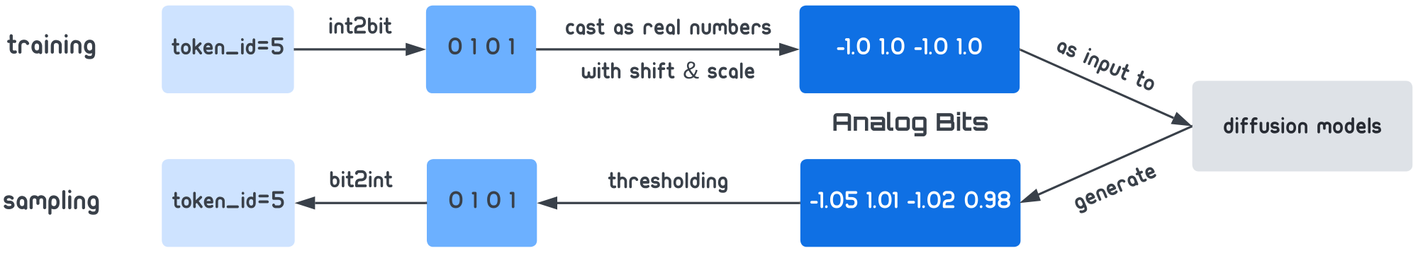
In this work, we propose a simple and generic approach for enabling continuous state diffusion models to generate discrete data. The key ingredient in our approach is analog bits: real numbers used to model the bits that represent the discrete data. Analog bits can be directly modeled by continuous state diffusion models, without requiring a discrete state space or re-formulation of the continuous diffusion process. At sampling time, the generated analog bits can be decoded into discrete variables by a simple thresholding operation. Our approach, as illustrated in Figure 1, is based on the following high-level conjecture. With strong continuous generative models (diffusion models in particular), it should not be too difficult to generate highly concentrated bimodal data where each real-valued analog bit is close to a binary bit. To reduce the prediction loss (such as negative log likelihood), the network has to model structures among analog bits that can actually lead to meaningful discrete variables after thresholding.

Besides analog bits, we further propose two simple techniques, namely Self-Conditioning and Asymmetric Time Intervals that greatly improve the sample quality. We evaluate the proposed approach on both discrete image generation, and image-conditional text / caption generation. On discrete $\textsc{Cifar-10}$ and $\textsc{ImageNet 64 $ \times $ 64}$ , the proposed Bit Diffusion model significantly improves both existing discrete diffusion models but also the best autoregressive model. For example, on categorical $\textsc{Cifar-10}$ , the best autoregressive model ([6]) obtains a FID of $12.75$, while our model (with $\frac{1}{3}$ of the model size of the autoregressive model, using 100 instead of 3072 sequential inference steps) achieves a much better $6.93$. For image captioning on MS-COCO dataset, our model achieves a result competitive with a strong autoregressive captioner based on a Transformer.

2. Method

Section Summary: Diffusion models, which generate data by gradually transforming random noise into realistic samples through a series of learned steps, typically work with continuous data but can be adapted for discrete types like text or categories. The method represents discrete values as binary bits converted into real numbers called "analog bits," allowing standard continuous diffusion processes to model them, followed by simple thresholding to recover the original binary format. To enhance generation quality, the approach incorporates self-conditioning, where the model uses its own prior predictions as input during sampling, and adjusts time intervals asymmetrically for better performance on these analog representations.

Preliminaries We start with a short introduction to diffusion models ([11, 12, 13, 16]). Diffusion models learn a series of state transitions to map noise $\bm \epsilon$ from a known prior distribution to $\bm x_0$ from the data distribution. To learn this (reverse) transition from the noise distribution to the data distribution, a forward transition from $\bm x_0$ to $\bm x_t$ is first defined:

$ \bm x_t = \sqrt{\gamma(t)} ~\bm x_0 + \sqrt{1-\gamma(t)} ~\bm \epsilon,\tag{1} $

where $\bm \epsilon \sim \mathcal{N}(\bm 0, \bm I)$, $t\sim \mathcal{U}(0, T)$ is a continuous variable, and $\gamma(t)$ is a monotonically decreasing function from 1 to 0. Instead of directly learning a neural net to model the transition from $\bm x_t$ to $\bm x_{t-\Delta}$, one can learn a neural net $f(\bm x_t, t)$ to predict $\bm x_0$ (or $\bm \epsilon$) from $\bm x_t$, and estimate $\bm x_{t-\Delta}$ from $\bm x_{t}$ and estimated $\tilde{\bm x}_0$ (or $\tilde{\bm \epsilon}$). This training of $f(\bm x_t, t)$ is based on denoising with a $\ell_2$ regression loss:

$ \mathcal{L}{\bm x_0} =\mathbb{E}{t\sim\mathcal{U}(0, T), \bm \epsilon\sim\mathcal{N}(\bm 0, \bm I)}|f(\sqrt{\gamma(t)} ~\bm x_0 + \sqrt{1-\gamma(t)} ~\bm \epsilon, t) - \bm x_0 |^2.\tag{2} $

To generate samples from a learned model, it follows a series of (reverse) state transition $\bm x_T\rightarrow \bm x_{T-\Delta} \rightarrow \cdots \rightarrow \bm x_0$. This can be achieved by iteratively applying denoising function $f$ on each state $\bm x_t$ to estimate $\bm x_0$, and then make a transition to $\bm x_{t-\Delta}$ with the estimated $\tilde{\bm x}_0$ (using transition rules such as those specified in DDPM ([12]) or DDIM ([13])). Note that state transitions in these diffusion models assume a continuous data space and state space. Therefore, one cannot directly apply it to model and generate discrete/categorical data.

Analog Bits A discrete data variable from an alphabet of size $K$ can be represented using $n=\lceil\log_2 K\rceil$ bits, as ${0, 1}^{n}$. Due to the discreteness, existing work has to re-formulate continuous diffusion models by adopting a discrete data space and state space ([11, 22, 23]). In contrast, we propose to simply cast the binary bits ${0, 1}^{n}$ into real numbers $\mathbb{R}^{n}$ for the continuous diffusion models [^1]. We term these real numbers analog bits since they learn to share the same bimodal values as binary bits but are modeled as real numbers. To draw samples, we follow the same procedure as sampling in a continuous diffusion model, except that we apply a quantization operation at the end by simply thresholding the generated analog bits. This yields binary bits which can be then converted into original discrete/categorical variables. Notably, there is no hard constraint to force the model to generate exact binary bits, but we expect a strong continuous generative model to generate real numbers that exhibit very clear bimodal concentrations and this is what happens in our experiments.

[^1]: After casting as real numbers, one may also transform them by shifting and scaling from $0, 1$ to $-b, b$.

For simplicity, we use the same regression loss function (Eq. 2) for modeling analog bits. However, it is possible to use other loss functions such as the cross entropy loss. We also note that the binary encoding mechanism for constructing analog bits is extensible as well (e.g., one-hot encoding). Extensions of loss functions and binary encoding are described in the Appendix B.

Self-Conditioning Conditioning is a useful technique for improving diffusion models ([24, 18]). However, a typical conditioning variable is either from some external sources, such as class labels ([24]) or low-resolution images from another network ([24, 25, 18]). Here we propose a technique for the model to directly condition on previously generated samples of its own during the iterative sampling process, which can significantly improve the sample quality of diffusion models.

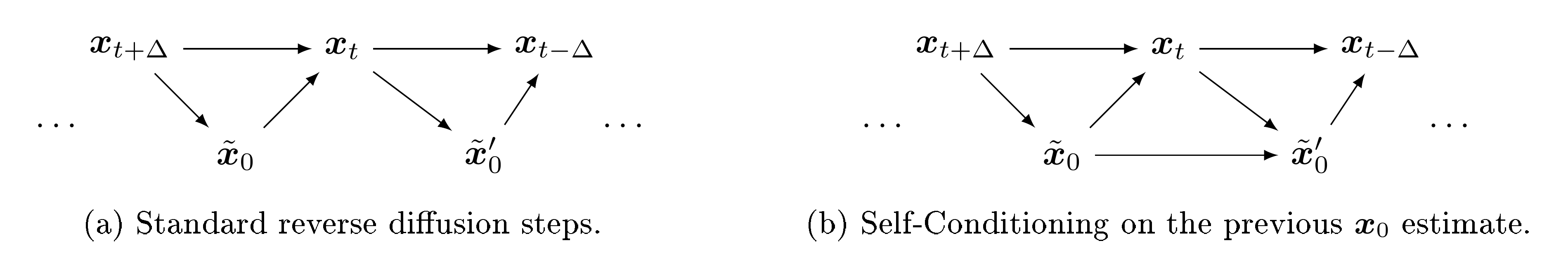
In a typical diffusion sampling process, the model iteratively predicts $\bm x_0$ (or $\bm \epsilon$) in order to progress the chain of mapping noise into data. However, as shown in Figure 2a, the previously estimated $\tilde{\bm x}_0$ is simply discarded when estimating $\bm x_0$ from a new time step, i.e. the denoising function $f(\bm x_t, t)$ does not directly depend on a previously estimated $\tilde{\bm x}_0$. Here we consider a slightly different denoising function of $f(\bm x_t, \tilde{\bm x}_0, t)$ that also takes previous generated samples as its input, illustrated in Figure 2b. A simple implementation of Self-Conditioning is to concatenate $\bm x_t$ with previously estimated $\tilde{\bm x}_0$. Given that $\tilde{\bm x}_0$ is from the earlier prediction of the model in the sampling chain, this comes at a negligible extra cost during sampling. In order to train the denoising function $f(\bm x_t, \tilde{\bm x}_0, t)$, we make some small changes to the training. With some probability (e.g., $50%$), we set $\tilde{\bm x}_0=\bm 0$ which falls back to modeling without Self-Conditioning. At other times, we first estimate $\tilde{\bm x}_0 = f(\bm x_t, \bm 0, t)$ and then use it for Self-Conditioning. Note that we do not backpropagate through the estimated $\tilde{\bm x}_0$ so the overall increase of training time is small (e.g., less than 25%).

Asymmetric Time Intervals Besides Self-Conditioning, we identify another factor, time step $t$, that can also impact Bit Diffusion models. Time step $t$ is an integral part of both denoising network $f(\bm x_t, t)$ as well as the state transitions. During a typical reverse diffusion process, the model takes symmetric time intervals (i.e., $\Delta$ as in $t\rightarrow t-\Delta$) for both the state transition and time reduction itself, resulting in the same/shared $t$ for both arguments of $f(\bm x_t, t)$. However, we find that, when taking large reverse steps, using asymmetric time intervals, implemented via a simple manipulation of time scheduling at generation, can lead to improved sampling quality for Bit Diffusion models.

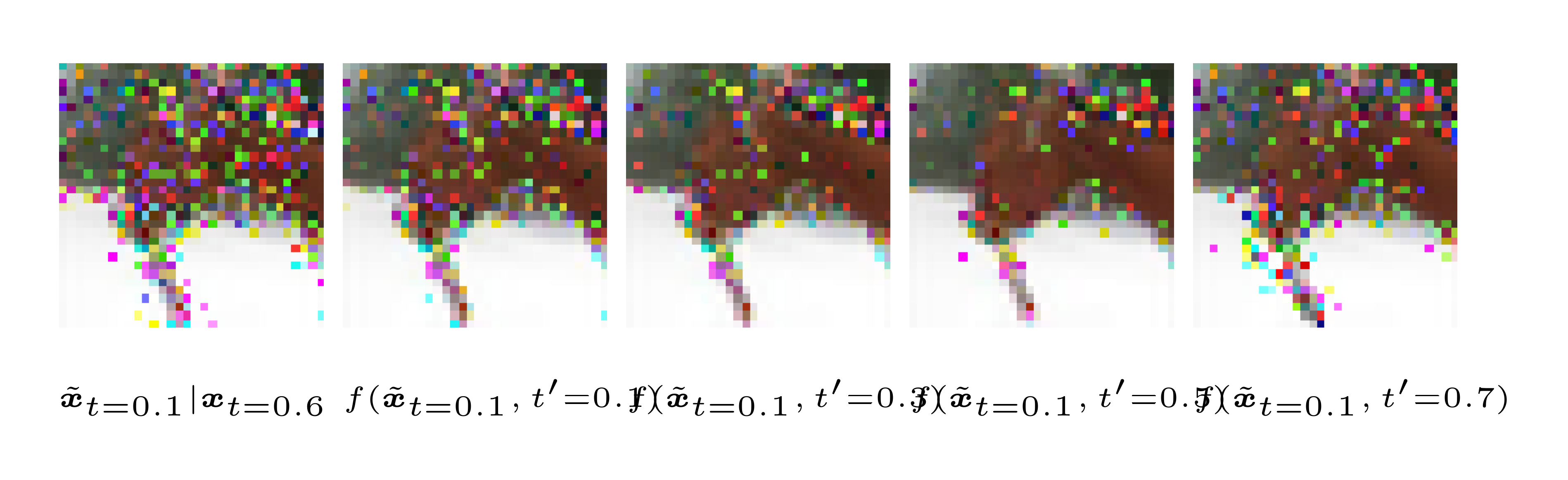
More specially, with asymmetric time intervals during the sampling process, we have $f(\bm x_t, t')$, where $t'=t+\xi$ and $\xi$ is a small non-negative time difference parameter. Note that training remains unchanged, and the same/shared $t$ is used for both arguments of the $f(\bm x_t, t)$. Figure 3 illustrates the effect with a trained Bit Diffusion model, where it is asked to take two reversing steps from a state $x_t$ constructed using the forward diffusion, and it shows that asymmetric time intervals reduce the number of noisy pixels (after thresholding and converting back to discrete variables).

Putting it together Algorithm 1 and Algorithm 2 summarize the training and sampling algorithms for the proposed Bit Diffusion model with Analog Bits, Self-Conditioning, and Asymmetric Time Intervals (via the td parameter). The proposed changes to the existing diffusion models are highlighted in blue. Note that unlike standard diffusion models ([11, 12, 24]), we use a continuous time parameterization between 0 and 1 instead of a fixed discrete time for maximal flexibility but they perform similarly. More details of the algorithm (including some important functions) can be found in Appendix A.

def train_loss(x):
  # Binary encoding: discrete to analog bits.
  x_bits = int2bit(x).astype(float)
  x_bits = (x_bits * 2 - 1) * scale

  # Corrupt data.
  t = uniform(0, 1)
  eps = normal(mean=0, std=1)
  x_crpt = sqrt(gamma(t)) * x_bits + 
              sqrt(1 - gamma(t)) * eps

  # Compute self-cond estimate.
  x_pred = zeros_like(x_crpt)
  if self_cond and uniform(0, 1) > 0.5:
    x_pred = net(cat([x_crpt, x_pred], -1), t)
    x_pred = stop_gradient(x_pred)

  # Predict and compute loss.
  x_pred = net(cat([x_crpt, x_pred], -1), t)
  loss = (x_pred - x_bits)**2
  return loss.mean()

def generate(steps, td=0):
  x_t = normal(mean=0, std=1)
  x_pred = zeros_like(x_t)

  for step in range(steps):
    # Get time for current and next states.
    t_now = 1 - step / steps
    t_next = max(1 - (step+1+td) / steps, 0)

    # Predict x_0.
    if not self_cond:
      x_pred = zeros_like(x_t)
    x_pred = net(cat([x_t,x_pred],-1), t_now)

    # Estimate x at t_next.
    x_t = ddim_or_ddpm_step(
        x_t, x_pred, t_now, t_next)

  # Binary decoding to discrete data.
  return bit2int(x_pred > 0)

3. Experiments

Section Summary: Researchers tested their Bit Diffusion method on two tasks: generating discrete images and creating captions for images. For image generation, they used datasets like CIFAR-10 and a smaller ImageNet version, encoding pixel values in binary formats such as standard 8-bit, gray code, or randomized bits, and measured quality with a metric called FID, where their approach outperformed other methods for discrete data. For captioning, they worked with the MS-COCO dataset, converting text tokens into bits and using a transformer model, achieving strong results compared to baselines.

We experiment with two different discrete data generation tasks, namely discrete/categorical image generation, and image captioning (image-conditional text generation).

3.1 Experimental Setup and Implementation Details

Datasets We use $\textsc{Cifar-10}$ ([26]) and $\textsc{ImageNet 64 $ \times $ 64}$ ([27]) [^2] for image generation experiments. We adopt widely used FID ([28]) as the main evaluation metric, and it is computed between 50K generated samples and the whole training set. For image captioning, following ([29]), we use MS-COCO 2017 captioning dataset ([30]).

[^2]: Following ([31, 24]), we center crop and area downsample images to 64 $\times$ 64.

Binary encoding Each pixel consists of 3 sub-pixels (RGB channels), and each sub-pixel is an integer in $[0, 256)$ representing the intensity. Standard continuous generative models cast RGB channels as real numbers and normalize them in $[-1, 1]$. For discrete image generation, we consider three discrete encoding for sub-pixels, namely $\textsc{uint8}$ , $\textsc{gray code}$ , and $\textsc{uint8 (rand)}$ . In $\textsc{uint8}$ , we use 8-bit binary codes converted from the corresponding sub-pixel integer in $[0, 256)$. In $\textsc{gray code}$ , we assign 8-bit binary codes uniquely to each sub-pixel integer such that two adjacent integers only differ by 1 bit. And in $\textsc{uint8 (rand)}$ , we assign 8-bit binary codes to every sub-pixel integer by randomly shuffling the integer-to-bits mapping in $\textsc{uint8}$ . The binary codes in $\textsc{uint8}$ and $\textsc{gray code}$ are loosely correlated with its original sub-pixel intensities, while $\textsc{uint8 (rand)}$ has no correlation so each sub-pixel is a categorical variable. The details of the binary codes and their correlations with sub-pixel intensity can be found in the Appendix C. We shift and scale the binary bits from $0, 1$ to $-1, 1$ for the analog bits.

For image captioning, we follow ([29]), and use sentencepiece ([32]) with a vocabulary of size 32K to tokenize the captions. After tokenization, we encode each token into 15 analog bits using the binary codes converted from the corresponding integer. We set the maximum number of tokens to 64 so the total sequence length is 960 bits. Since we directly model bits, it is also possible to directly work with their byte representations without a tokenizer, but we leave this for future work.

Architecture We use the U-Net architecture ([12, 24, 33]) for image generation. For $\textsc{Cifar-10}$ , we use a single channel dimension of 256, 3 stages and 3 residual blocks ([34]) per stage, with a total of 51M parameters. We only use dropout ([35]) of 0.3 for continuous diffusion models on $\textsc{Cifar-10}$ . For $\textsc{ImageNet 64 $ \times $ 64}$ , following ([24]), we use a base channel dimension of 192, multiplied by 1, 2, 3, 4 in 4 stages and 3 residual blocks per stage, which account for a total of 240M parameters [^3]. For $\textsc{uint8 (rand)}$ encoding, we find the following "softmax factorization" architectural tweak on the final output layer can lead to a better performance. Instead of using a linear output layer to predict analog bits directly, we first predict a probability distribution over 256 classes per sub-pixel (with each class corresponds to one of the 256 different 8-bit codes), and then map class distribution into analog bits by taking weighted average over all 256 different 8-bit codes.

[^3]: Our model is about 30M parameters smaller than that used in ([24]) as we drop the middle blocks for convenience, which may have a minor effect on performance.

For image captioning, we follow the architecture used in ([36, 29]), with a pre-trained image encoder using the object detection task, for both autoregressive baseline as well as the proposed method. Both decoders are randomly initialized 6-layer Transformer ([10]) decoder with 512 dimension per layer. For the autoregressive decoder, the token attention matrix is offset by the causal masks, but it is non-masked all-to-all attention for our Bit Diffusion.

Other settings We train our models with the Adam optimizer ([37]). For $\textsc{Cifar-10}$ , we train the model for $1.5$ M steps with a constant learning rate of $0.0001$ and batch size of $128$. For $\textsc{ImageNet 64 $ \times $ 64}$ , we train the model for 500K steps with a constant learning rate of $0.0002$ [^4] and batch size of $1024$. For Bit Diffusion, we use Self-Conditioning by default, unless otherwise specified. We use an exponential moving average of the weights during training with a decay factor of $0.9999$. For our best image generation results, we sweep over a few sampling hyper-parameters, such as sampler (DDIM vs DDPM), sampling steps in ${100, 250, 400, 1000}$, and time difference in ${0., 0.01, 0.1, 0.2, 0.5}$.

[^4]: For $\textsc{uint8 (rand)}$ encoding, we use learning rate of $0.0001$ instead.

3.2 Discrete Image Generation

\begin{tabular}{lccc}
  \toprule
  \multirow{2}{*}{Method} & \multirow{2}{*}{State space} & FID & FID \\ 
  && (Unconditional)&(Conditional) \\
  \midrule
  \textit{On continuous pixels (as reference):\hfill} & &\\
  DDPM ([12]) & Continuous & $3.17$ & - \\
  DDPM (our reproduction) & Continuous & $\mathbf{3.14}$ & $\mathbf{2.95}$ \\
  \midrule
  \textit{On discrete (partial) ordinal pixels:\hfill} & &\\
  D3PM Gauss+Logistic ([23]) & Discrete & $7.34$ & - \\
  $\tau$ LDR-10 ([38]) & Discrete & $3.74$ & - \\
  Bit Diffusion on \textsc{uint8} & Continuous & $\mathbf{3.48}$ & $\mathbf{2.72}$ \\
  Bit Diffusion on \textsc{gray code} & Continuous & $3.86$ & $2.94$ \\
  \midrule
  \textit{On categorical pixels:\hfill} & &\\
  D3PM uniform ([23]) & Discrete & $51.27$ & - \\
  D3PM absorbing ([23]) & Discrete & $30.97$ & - \\
  Autoregressive Transformer ([6]) & Discrete & $12.75$ & - \\
  Bit Diffusion on \textsc{uint8 (rand)} & Continuous & $\mathbf{6.93}$ & $\mathbf{6.43}$ \\
  \bottomrule
  \end{tabular}

\begin{tabular}{cccc}
  \toprule
  DDPM (our repo.) & Bit Diffusion & Bit Diffusion & Bit Diffusion\\
  on continuous pixels & on \textsc{uint8} & on \textsc{gray code} & on \textsc{uint8 (rand)}\\ 
  \midrule
  $3.43$ & $4.84$ & $5.14$ & $8.76$ \\
  \bottomrule
  \end{tabular}

We compare our model against state-of-the-art generative models ([12, 23, 38, 6]) on generating discrete $\textsc{Cifar-10}$ images in Table 1. Our model achieves better results compared to both existing discrete diffusion models and the best autoregressive model. When compared to continuous diffusion models (i.e., DDPM), our Bit Diffusion models on $\textsc{uint8}$ and $\textsc{gray code}$ can achieve similar performance.

Discrete generation of $\textsc{ImageNet 64 $ \times $ 64}$ is significantly harder than $\textsc{Cifar-10}$ , and we have not found other competing methods that report FIDs, so we only compare the proposed method against DDPM on continuous pixels. Results are shown in Table 2. We find that the diffusion model on continuous pixels has the best FID while the diffusion model on $\textsc{uint8 (rand)}$ , i.e., categorical data, has the worst FID, indicating the increase of hardness when removing intensity/order information in sub-pixels. Note that, in these experiments, there is no extra model capacity to compensate for the loss of intensity/order information since the model sizes are the same. Figure 4 shows generated images of different diffusion models on continuous and discrete $\textsc{ImageNet 64 $ \times $ 64}$ . Despite the differences in FIDs, visually these samples look similar.

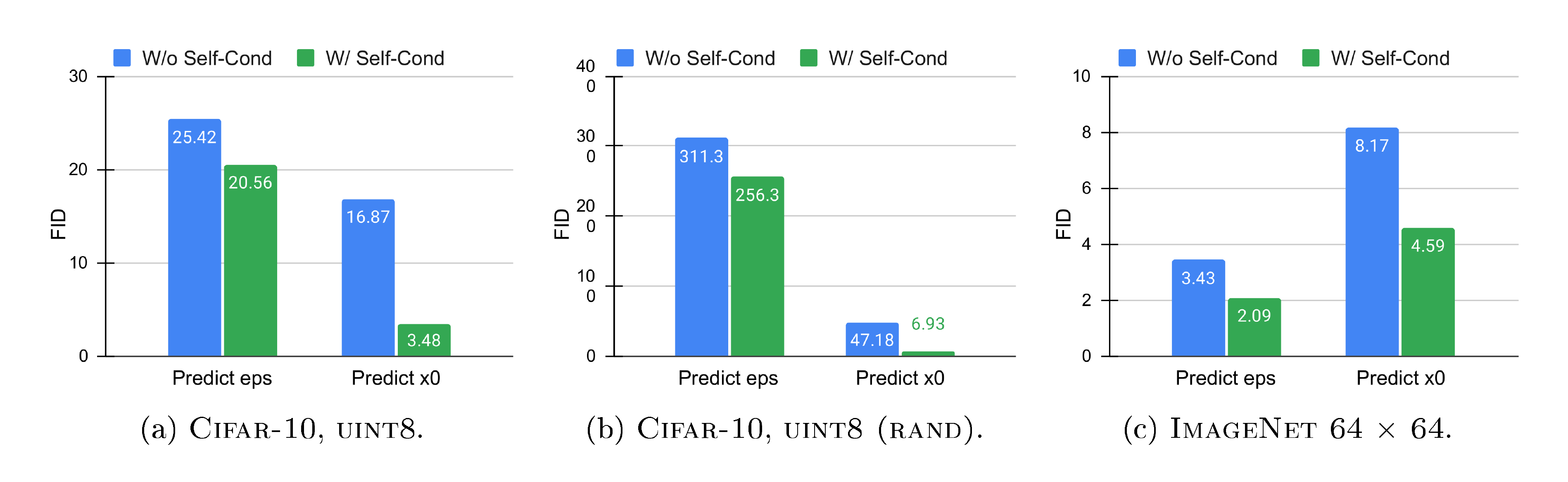
Ablation of Self-Conditioning Figure 5 shows the effectiveness of the Self-Conditioning technique in both Bit Diffusion and continuous diffusion models. Note that the experiments are performed in three settings, namely $\textsc{Cifar-10}$ with $\textsc{uint8}$ , $\textsc{Cifar-10}$ with $\textsc{uint8 (rand)}$ , and $\textsc{ImageNet 64 $ \times $ 64}$ with continuous pixels, where the only difference for pairs in each setting is whether the Self-Conditioning is used. For $\textsc{Cifar-10}$ , we find that Self-Conditioning greatly improves the performance across different binary encodings. We also notice that for Bit Diffusion, predicting $\bm x_0$ is much more effective than predicting $\bm \epsilon$. For $\textsc{ImageNet 64 $ \times $ 64}$ , we find that the proposed Self-Conditioning also leads to improved FIDs for continuous diffusion (i.e., DDPM). Therefore, we conclude that Self-Conditioning by itself is a generic technique that can benefit diffusion models on both continuous and discrete data.

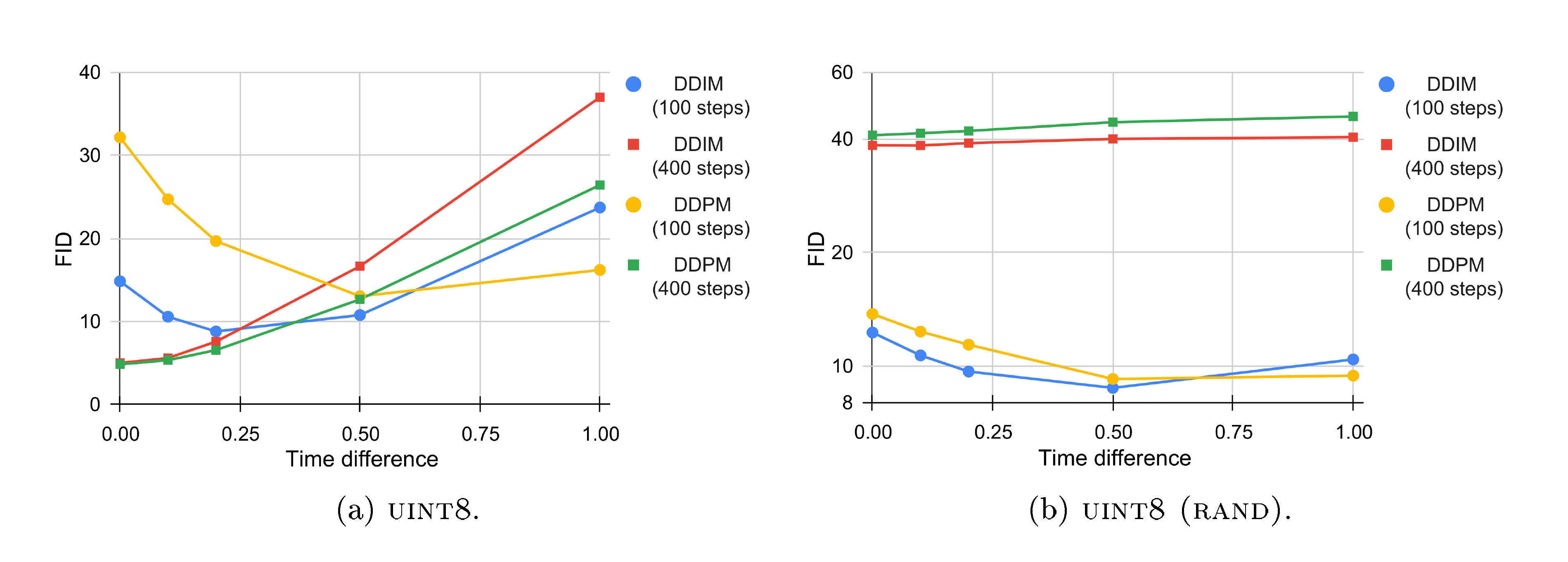
Ablation of asymmetric time intervals Figure 6 shows the FID on generated $\textsc{ImageNet 64 $ \times $ 64}$ samples as we vary the time difference parameter during the sampling process. We find that as the number of steps increases (from $100$ to $400$), the optimal time difference shrinks to $0$. For $100$ steps, a non-zero time difference leads to a significant improvement of FID. We also note that for Bit Diffusion on $\textsc{uint8 (rand)}$ , using $400$ sampling steps actually leads to a drastically worse sample quality than using $100$ steps. This is related to how the Self-Conditioning is applied and we present alternative Self-Conditioning sampling strategies in the Appendix G, some of which lead to improved FIDs at a cost of longer sampling time.

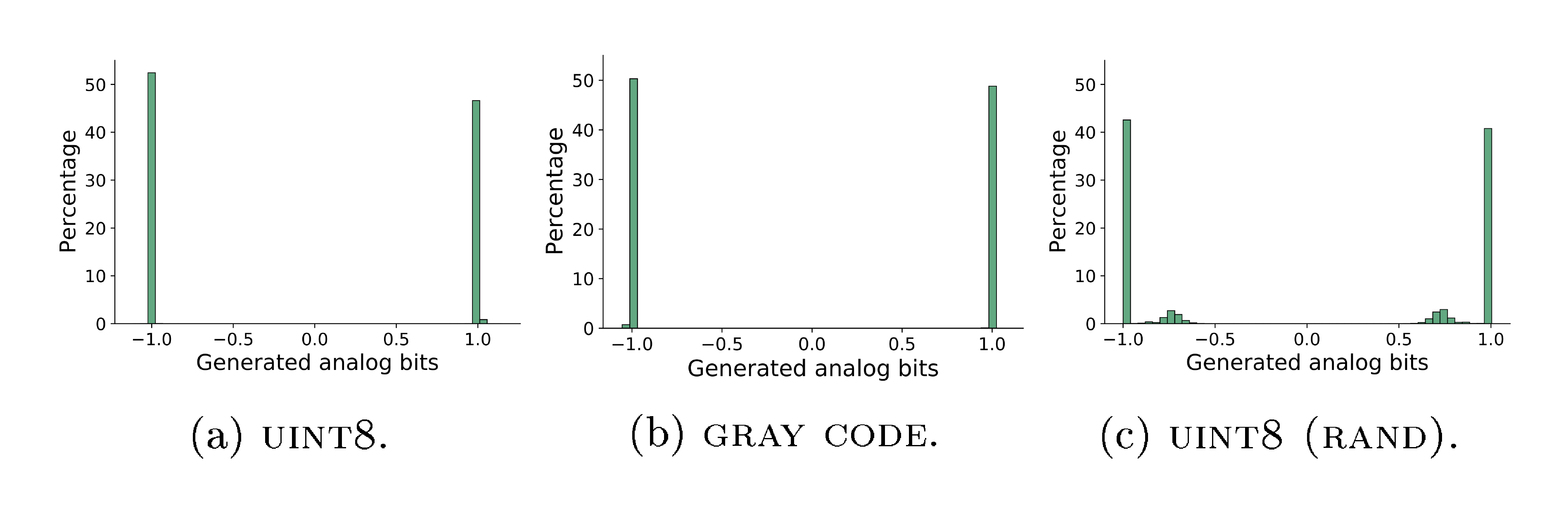
Concentration of generated analog bits Figure 7 visualizes the distribution of generated analog bits from $64$ generated images on $\textsc{ImageNet 64 $ \times $ 64}$ . Although there is no hard constraint on the analog bits being binary / bimodal, the generated ones are highly concentrated on two modes, which makes the thresholding / quantization easy and robust.

3.3 Image Captioning

We compare our Bit Diffusion model with an autoregressive Transformer baseline ([29]). As mentioned, both models have similar architectures, with an object detection pretrained ([36]) image encoder, and a randomly initialized Transformer ([10]) decoder. Table 3 presents the main comparison. Overall, our model achieves similar performance as the autoregressive model. We find that generally it only needs about 10 steps for the model to achieve good results, despite that there are a total of maximum 960 bits for caption that the model has to model. We find that the asymmetric time intervals play an important role in the final performance of our model, as demonstrated in Table 4, especially when sampling steps are fewer.

\begin{tabular}{c|ccc}
  \toprule
  Method & BLEU-4 & CIDEr & ROUGE-L \\
  \midrule
  Autoregressive Transformer & $33.9$ & $\mathbf{1.18}$ & $0.57$ \\ 
  \midrule
  Bit Diffusion (5 steps) & $31.5$ & $1.00$ & $0.55$ \\
  Bit Diffusion (10 steps) & $34.5$ & $1.13$ & $0.57$ \\
  Bit Diffusion (20 steps) & $\mathbf{34.7}$ & $1.15$ & $\mathbf{0.58}$ \\
  Bit Diffusion (40 steps) & $34.4$ & $1.15$ & $0.57$ \\
  \bottomrule
  \end{tabular}

\begin{tabular}{c|ccccccccc}
  \toprule
  & \multicolumn{9}{c}{Time difference} \\
  & $0.0$ & $1.0$ & $2.0$ & $3.0$ & $4.0$ & $5.0$ & $6.0$ & $7.0$ & $8.0$ \\
  \midrule
  $5$ steps & $17.1$ & $27.8$ & $30.8$ & $31.5$ & $\mathbf{31.6}$ & $31.5$ & $31.5$ & $31.5$ & $\mathbf{31.6}$ \\
  $10$ steps & $17.6$ & $26.3$ & $30.7$ & $32.6$ & $33.4$ & $34.0$ & $34.3$ & $34.5$ & $\mathbf{34.6}$ \\
  $20$ steps & $20.0$ & $27.9$ & $30.6$ & $32.0$ & $32.3$ & $33.9$ & $34.4$ & $\mathbf{34.7}$ & $34.5$ \\
  $40$ steps & $20.7$ & $27.5$ & $30.7$ & $32.2$ & $32.9$ & $33.2$ & $33.8$ & $\mathbf{34.4}$ & $\mathbf{34.4}$ \\
  \bottomrule
  \end{tabular}

Table 5 provides some generated samples of our model when different inference steps are used. The model makes mistakes when the sampling steps are too few, and the mistakes may not always be interpretable due to that the model directly predicts the bits behind the tokenized word pieces and a small difference in bits can lead to total different words.

:::

Table 5: Generated image captions under different number of sampling steps.

:::

4. Related Work

Section Summary: Autoregressive models excel at generating discrete data like text and low-resolution images but struggle with high computational costs as data size grows. Diffusion models, normalizing flows, and other approaches like VAEs and GANs have been adapted for discrete data through various embeddings and transformations, yet they often face limitations in flexibility, efficiency, or performance compared to the simpler, more scalable method proposed here. The technique's self-conditioning also echoes elements of self-modulation in GANs and denoising strategies in other models.

Autoregressive models for discrete data Autoregressive models have demonstrated state-of-the-art results when it comes to generating discrete data. In particular, text generation, or language modeling, is dominated by autoregressive approaches ([7, 8, 9]). Autoregressive models are also applied to discrete/categorical image generation ([1, 2, 3, 4, 5, 6, 39]), where they work well on small image resolutions. However, the computation cost and memory requirement increase drastically (typically in a quadratic relation) as the size of sequence or the image resolution increase, so it becomes very challenging to scale these approaches to data with large dimensions.

Diffusion models for discrete data State-of-the-art diffusion models ([17, 18, 19, 20, 21]) cannot generate discrete or categorical data. Existing extensions of these continuous diffusion models to discrete data are based on both discrete data space and state space ([11, 22, 23, 38]). Compared to discrete state space, continuous state space is more flexible and potentially more efficient. Our approach is also compatible with both discrete and continuous time, and does not require re-formulation of existing continuous models, thus it is simpler and can potentially be plugged into a broader family of generative models.

Another line of discrete diffusion models is based on the embedding of discrete data ([40]). One can also consider our binary encoding with analog bits as a simple fixed encoder, and the decoding / quantization of bimodal analog bits is easy and robust via a simple thresholding operation. In contrast, the quantization of real numbers in generated continuous embedding vectors may contain multiple modes per dimension, leading to potential difficulty in thresholding/quantization.

Normalizing Flows for discrete data Normalizing Flows ([41, 42, 43]) are a powerful family of generative models for high-dimensional continuous distributions based on some invertible mapping. However, straightforward application of flow-based models on categorical data is limited due to the inherent challenges on discrete support. Discrete flows ([44, 45, 46]) introduce invertible transformations of random variables in discrete space without the need of computing the log-determinant of Jacobian. Other works ([47, 22, 48]) introduce various embedding methods for transforming discrete data into continuous space with disjoint support, which can be interpreted as a variational inference problem ([49]) with different dequantization distribution families. Several works ([50, 51, 52]) also explore normalizing flows on discrete data under the Variational Autoencoders ([53]) framework by enriching the prior. Compared to our diffusion-based approach, these models suffer from strict invertible restrictions on network architecture, thus limiting their capacity.

Other generative models for discrete data Other generative models, such as Varational Autoencoders (VAE) ([53]), Generateive Adversarial Networks (GAN) ([54, 55, 56, 57, 58]) have also been applied to generate discrete data. These methods have not yet achieved the level of performance as autoregressive models on tasks such as discrete image generation or text generation, in terms of sample quality or data likelihood. Potentially, the proposed analog bits can also be applied to these continuous generative models, by having the networks directly model and generate analog bits, but it is not explored in this work.

Other related work The proposed Self-Conditioning technique shares some similarities with self-modulation in GANs ([59]) (where the earlier latent state can directly modulate the later latent states) and SUNDAE ([60]) (where an inference step is incorporated for denoising).

5. Conclusion

Section Summary: The researchers present a straightforward method that allows diffusion models, typically used for continuous data, to create discrete or categorical data by converting it into "analog bits" and refining the process with techniques like self-conditioning and asymmetric time intervals for better results. This approach achieves top performance in generating discrete images, surpassing autoregressive models, and performs competitively in tasks like creating text descriptions for images from the MS-COCO dataset. While it shares the drawback of needing many steps to produce high-quality outputs, similar to other diffusion models, the team anticipates that advances in continuous data handling will enhance this discrete application too.

We introduce a simple and generic technique that enables continuous state diffusion models to generate discrete data. The main idea is to encode discrete or categorical data into bits and then model these bits as real numbers that we call analog bits. We also propose two simple techniques, namely Self-Conditioning (i.e., condition the diffusion models directly on their previously generated samples) and Asymmetric Time Intervals, that lead to improved sample quality. We demonstrate that our approach leads to state-of-the-art results in discrete / categorical image generation, beating the best autoregressive model. In an image-conditional text generation task on MS-COCO dataset, we also achieve competitive results compared to autoregressive models. One limitation of our approach, similar to other existing diffusion models, is that they still require a significant number of inference steps for generating good (image) samples. However, we expect that future improvements from diffusion models for continuous data can also transfer to discrete data using analog bits.

Acknowledgements

Section Summary: The authors express thanks to Priyank Jaini and Kevin Swersky for providing valuable feedback on their draft. They also acknowledge that their implementation draws partly from the Pix2Seq codebase and thank Lala Li and Saurabh Saxena for their work on it.

We would like to thank Priyank Jaini, Kevin Swersky for providing helpful feedback to our draft. Our implementation is partially based on the Pix2Seq codebase, and we thank Lala Li, Saurabh Saxena, for their contributions to the Pix2Seq codebase.

Appendix

Section Summary: The appendix offers deeper technical insights into the paper's methods, including Python code for converting integers to binary bits and vice versa, as well as steps for updating diffusion models using DDIM and DDPM rules to estimate image states over time. It explores alternative approaches like one-hot encoding for discrete data, which uses more bits but allows for softmax-based training, and tests various loss functions such as sigmoid cross-entropy, showing promising results on image datasets like CIFAR-10 through quality scores. Additionally, it details pixel encodings like standard uint8, gray code, and a randomized version that scrambles order information, illustrated by correlations between pixel differences and binary bit distances to highlight how these preserve or remove intensity patterns.

A. More Details of Algorithm 1 and 2

Algorithm 3 and Algorithm 4 provide more detailed implementations of functions in Algorithm 1 and Algorithm 2.

import tensorflow as tf

def int2bit(x, n=8):
  # Convert integers into the corresponding binary bits.
  x = tf.bitwise.right_shift(tf.expand_dims(x, -1), tf.range(n))
  x = tf.math.mod(x, 2)
  return x

def bit2int(x):
  # Convert binary bits into the corresponding integers.
  x = tf.cast(x, tf.int32)
  n = x.shape[-1]
  x = tf.math.reduce_sum(x * (2 ** tf.range(n)), -1)
  return x

def gamma(t, ns=0.0002, ds=0.00025):
  # A scheduling function based on cosine function.
  return numpy.cos(((t + ns) / (1 + ds)) * numpy.pi / 2)**2

def ddim_step(x_t, x_pred, t_now, t_next):
  # Estimate x at t_next with DDIM updating rule.
  γnow = gamma(t_now)
  γnext = gamma(t_next)
  x_pred = clip(x_pred, -scale, scale)
  eps = 1 / sqrt(1 - γnow) * (x_t - sqrt(γnow) * x_pred)
  x_next = sqrt(γnext) * x_pred + sqrt(1 - γnext) * eps
  return x_next

def ddpm_step(x_t, x_pred, t_now, t_next):
  # Estimate x at t_next with DDPM updating rule.
  γnow = gamma(t_now)
  αnow = gamma(t_now) / gamma(t_next)
  σnow = sqrt(1 - αnow)
  z = normal(mean=0, std=1)
  x_pred = clip(x_pred, -scale, scale)
  eps = 1 / sqrt(1 - γnow) * (x_t - sqrt(γnow) * x_pred)
  x_next = 1 / sqrt(αnow) * (x_t - (1 - αnow) / sqrt(1 - γnow) * eps) + σnow * z
  return x_next

B. Alternative Binary Encoding and Loss Functions

B.1 Analog Bits based on One-Hot Encoding

An alternative binary encoding to the base-2 encoding of the discrete data used in the main paper, is the one-hot encoding, where a discrete variable is represented as a vector whose length is the same as the vocabulary size $K$, with a single slot being $1$ and the rest being $0$. The resulting one-hot vector can be similarly treated as analog bits and modeled by continuous state diffusion models. To obtain discrete variables corresponding to the generated analog bits, we use an $\operatorname{arg, max}$ operation over all candidate categories, instead of the thresholding operation in base-2 analog bits. Note that the one-hot encoding requires $K$ bits, which is less efficient compared to base-2 encoding that only requires $\lceil\log_2 K\rceil$ bits, especially for large $K$. [^5]

[^5]: Although, one can reduce the vocabulary size $K$ by using sub-tokenization (e.g., subword ([61])), or learned discrete codes ([62, 63]).

B.2 Sigmoid Cross Entropy Loss

As we use $\ell_2$ loss by default for its simplicity and compatibility with continuous diffusion models. The proposed Bit Diffusion models can work with other loss functions too. Since the analog bits are bimodal, we can use the following sigmoid cross entropy loss:

$ \mathcal{L}_{\bm x_0, \bm x_t, t} = \log\sigma(\bm x_0 f(\bm x_t, t)), $

where we assume $\bm x_0 \in {-1, 1}^n$, and $\sigma$ is a sigmoid function. During the sampling process, we use $2\sigma(f(\bm x_t, t))-1$ as the output of denoising network.

B.3 Softmax Cross Entropy Loss

For one-hot analog bits, one could also add a softmax activation function for the output of denosing network $f$, and use the following softmax cross entropy loss:

$ \mathcal{L}_{\bm x_0, \bm x_t, t} = \bm x_0 \log \text{softmax}(f(\bm x_t, t)), $

where we assume $\bm x_0 \in {0, 1}^n$ which is the one-hot representation.

B.4 Preliminary Experiments

Table 6 presents FIDs of Bit Diffusion models with different types of analog bits and loss functions on unconditional $\textsc{Cifar-10}$ . Note that it is possible some of these results can be improved by more tuning of hyper-parameters or tweaks of the network, but we do not focus on them in this work.

:Table 6: FIDs of Bit Diffusion models with different types of analog bits and loss functions on unconditional $\textsc{Cifar-10}$.

	$\ell_2$ loss	Logistic loss	Softmax loss
$\textsc{one hot}$	$46.32$	$26.82$	$29.49$
$\textsc{uint8}$	$3.48$	$3.53$	-
$\textsc{gray code}$	$3.86$	$3.71$	-
$\textsc{uint8 (rand)}$	$6.93$	$49.29$	-

C. On Binary Encoding of Pixels: $\textsc{uint8}$, $\textsc{gray code}$, $\textsc{uint8 (rand)}$

In the main paper, we describe three different types of binary encodings of pixels. Here we provide additional detail on how we generate $\textsc{uint8 (rand)}$ : we first apply a random permutation to 256 sub-pixel values, and then assign the binary binary bits of permuted integers to the non-permuted integers. For example, assume 0 is mapped to 228 after the permutation, the analog bits of 0 would be the binary bits of 228. The random permutation is generated by numpy.random.seed(42); numpy.random.shuffle(numpy.arange(256)).

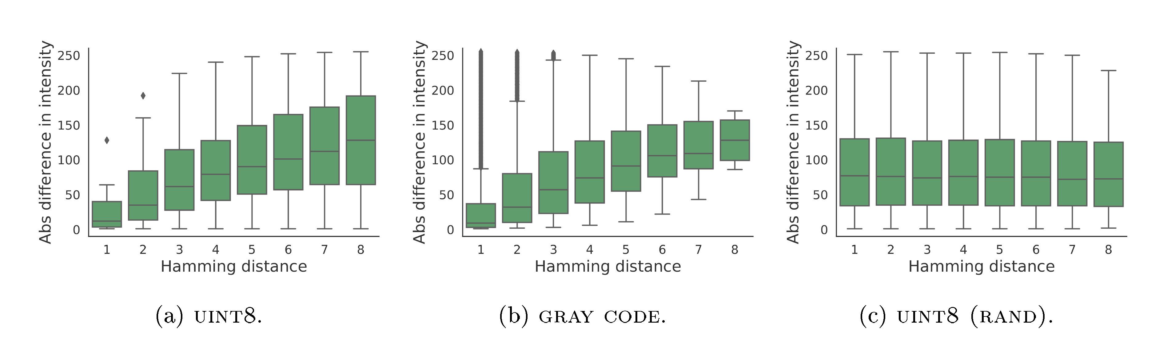
Figure 8 show the correlation between Hamming distance of three different binary encodings we use and the (absolute) difference of sub-pixel intensity. This is done by taking every pair of subpixel integers (in $[0, 256)$), compute their absolute difference, as well as the Hamming distance between the corresponding binary bits. We find that both $\textsc{uint8}$ and $\textsc{gray code}$ exhibit partial correlation between the two quantities (with different correlation patterns), meaning that these codes partially contain the order information about the original sub-pixel intensity. However, $\textsc{uint8 (rand)}$ exhibits no correlation between hamming distance and sub-pixel intensity, indicating the order information is fully removed, thus can be considered as categorical data.

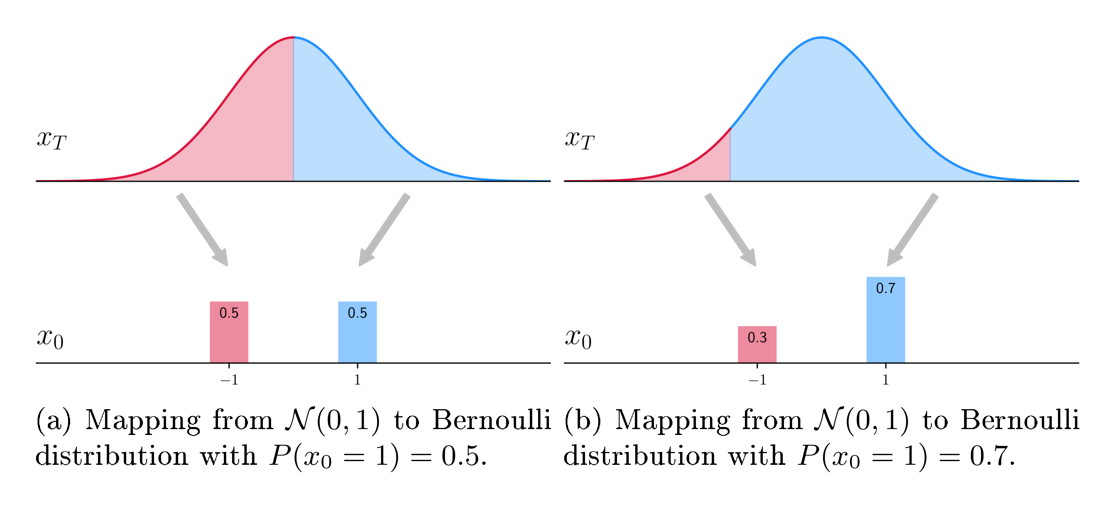
D. A Toy Example on Continuous Modeling of Discrete Variables

An intuitive toy example of how a continuous generative model can generate binary data is given in Figure 9, where a mapping from prior distribution at $\bm x_T$ to data distribution at $\bm x_0$ is shown. With a deterministic sampler (such as DDIM), it is straight-forward how they can represent any Bernoulli distribution by dividing the prior into two regions of probability densities corresponding to the Bernoulli distribution. For stochastic samplers, they can achieve a similar effect but the mapping from noise to data is stochastic. For an arbitrary discrete variable, represented as m-dimensional Bernoulli distribution, the mapping from continuous noise distribution to the target Bernoulli distribution also exists but it is more complicated (and difficult to visualize).

E. On Other Samplers for Continuous Diffusion Models

As our models are based on continuous diffusion models, in theory our models are able to incorporate faster samplers. To this end, we conduct preliminary exploration of using DPM-Solver ([64]) for sampling some of our models.

We find that DPM-Solver provides a boost to diffusion models based on analog bits, similar to what it is able to do for continuous data. This shows a potential of our model enjoying faster continuous sampler while other baselines (e.g., D3PM) may not be able to do due to their use of discrete states. Table 7 below shows the FID scores of bit diffusion models on ImageNet-64x64 under different binary encoding schemes. We find that the DPM-Solver is able to provide a significant reduction in function evaluations for bit diffusion on discrete/categorical data (with 30 NFEs it gets comparable FIDs as 100 NFEs of DDIM), similar to that in continuous diffusion models.

\begin{tabular}{lccc}
\toprule
{Samplers} & {UINT8} & {Gray Code} & {UINT8 (RAND)} \\
\midrule
DDIM @ 1000 NFE & 5.51 & 5.14 & 58.45 \\
DDPM @ 1000 NFE & 7.71 & 6.91 & 64.08 \\
DDIM @ 400 NFE & 5.00 & 5.52 & 38.44 \\
DDPM @ 400 NFE & 4.84 & 5.37 & 40.91 \\
DDIM @ 100 NFE & 8.80 & 11.31 & 8.76 \\
DDPM @ 100 NFE & 13.04 & 12.77 & 9.25 \\
\midrule
DPM-Solver @ 30 NFE & 7.85 & 9.64 & 10.39 \\
DPM-Solver @ 50 NFE & 6.46 & 7.61 & 10.96 \\
\bottomrule
\end{tabular}

Furthermore, we also find that self-conditioning continues to provide a boost with DPM-solver. For example, the Table 8 shows FID scores of diffusion models on ImageNet 64x64 (continuous rgb values). And we find that the self-conditioning consistently improves the performance of DPM-Solver with fixed number of function evaluations.

\begin{tabular}{c|c|c}
\toprule
{Model} & {DPM-Solver @ 20 NFE} & {DPM-Solver @ 30 NFE} \\
\midrule
$\epsilon$ prediction, w/o self-conditioning & 6.10 & 5.58 \\
$\epsilon$ prediction, w/ self-conditioning & 4.24 & 4.15\\
\midrule
$x_0$ prediction, w/o self-conditioning & 12.13 & 11.05 \\
$x_0$ prediction, w/ self-conditioning & 6.94 & 6.43 \\
\bottomrule
\end{tabular}

F. Extra Random Samples on $\textsc{Cifar-10}$ and $\textsc{ImageNet 64 $ \times $ 64}$

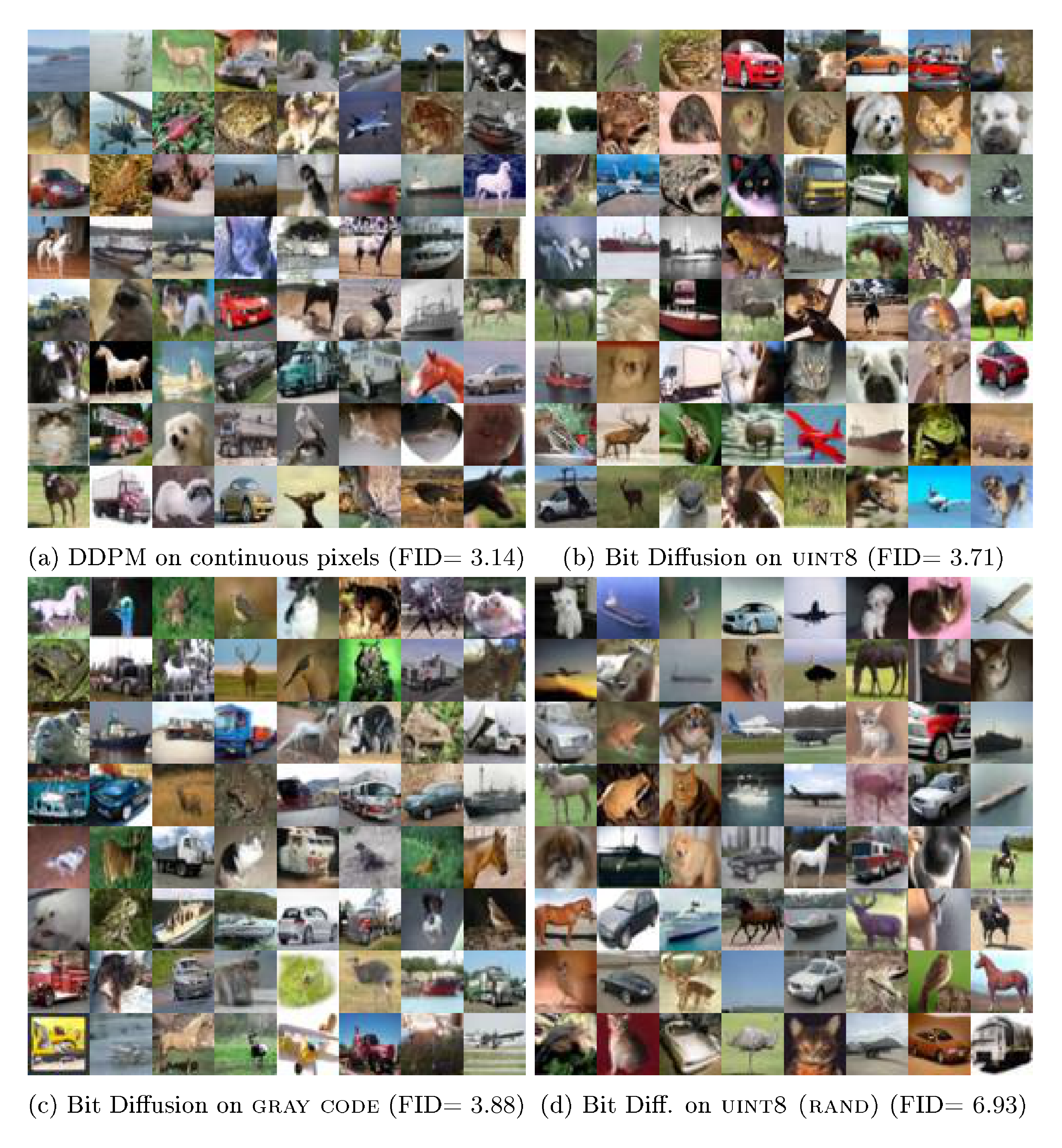
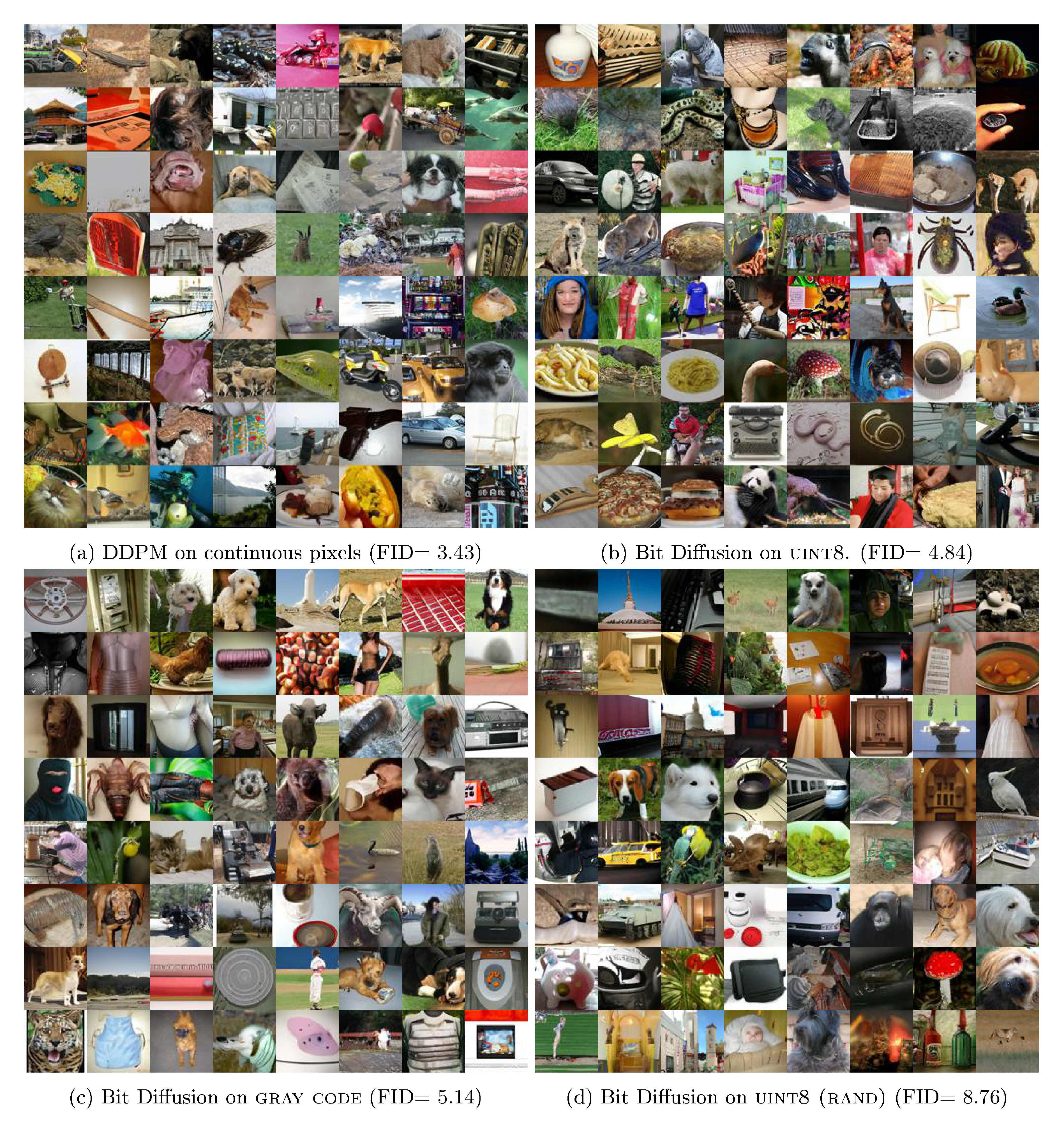
Figure 10 shows random samples (non cherry-picked) from unconditional diffusion models on $\textsc{Cifar-10}$ with continuous pixels and analog bits.

Figure 11 shows random samples (non cherry-picked) from class-conditional diffusion models on $\textsc{ImageNet 64 $ \times $ 64}$ with continuous pixels and analog bits.

G. On Sampling Strategies with Self-Conditioning

G.1 Method

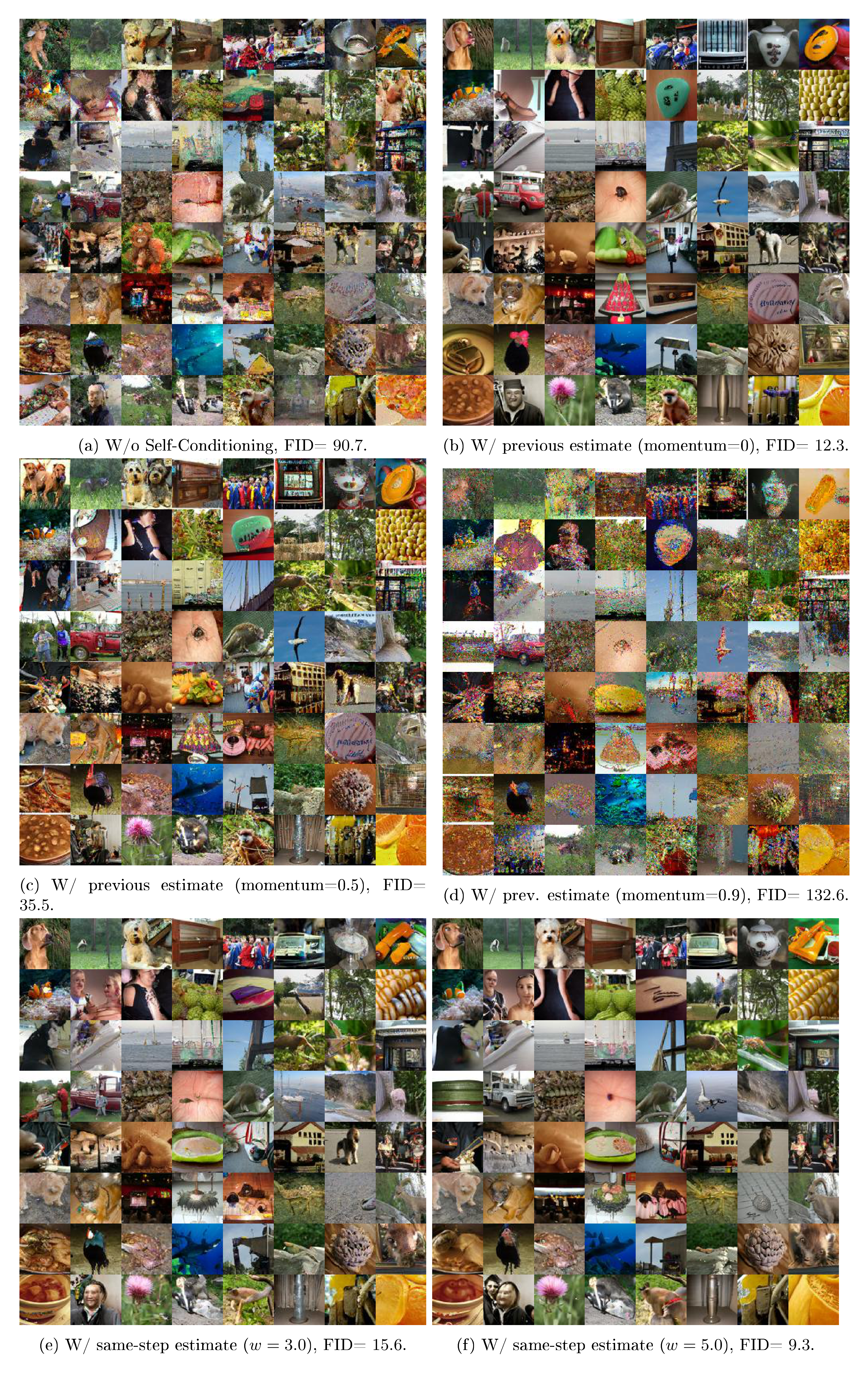
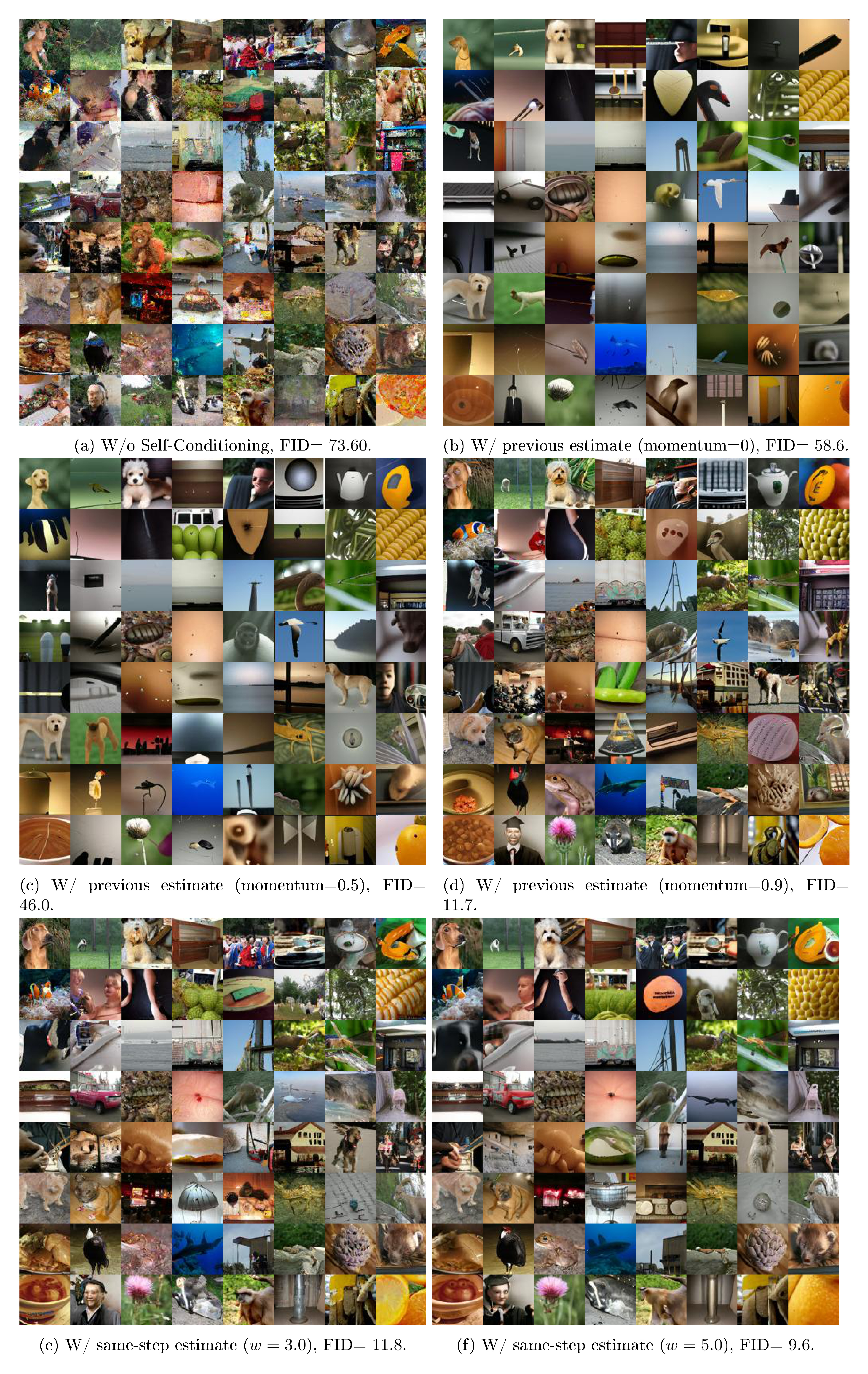
In this section, we present extensions to the default sampling strategy with Self-Conditioning in Algorithm 2. The default sampling strategy utilizes data estimate from the previous step as the conditional input to the denoising network for producing data estimate at the current step. While this is both simple and effective, we observe that, for $\textsc{uint8 (rand)}$ encoding of pixels, as the number of sampling steps increases (with both DDIM or DDPM samplers), the generated samples tend to be over-smoothed. We propose the following two extensions of the default sampling strategy to mitigate the issues and provide improvements when using larger sampling steps.

Self-Conditioning based on Momentum Estimate The first extension to the default sampling strategy is to adopt an exponential moving average over the previous data estimate to provide a more reliable conditioning input, similar to a momentum optimizer. The detailed procedure is shown in Algorithm 5, where the differences from the default sampling strategy are highlighted in blue. Note that the default sampling strategy can also be considered as a special case of this generalized form in that the momentum is set to zero.

Self-Conditioning based on Self-Guidance One potential issue with the default sampling strategy is the slight discrepancy of the Self-Conditioning signal during training and inference/sampling. Specifically, during training, the Self-Conditioning signal is the data estimate from the same time step, while, during sampling, it is from the past time step(s). Therefore, here we propose an approach that also use the same step data estimate for self-conditioning, which comes at the cost of extra forward pass over the denoising network at sampling time. Specifically, we conduct two forward passes of denoising network per sampling step, one with zero data estimate and the other with current data step estimate, and then we use a weighted combination, similar to ([65]), of both prediction to form the final prediction at the current step. The detailed procedure is given in Algorithm 6 with differences to the default sampling strategy highlighted.

def generate(steps, td=0, momentum=0.):
  x_t = normal(mean=0, std=1)
  x_pred = zeros_like(x_t)
  x_accu = zeros_like(x_t)

  for step in range(steps):
    # Get time for current and next states.
    t_now = 1 - step / steps
    t_next = max(1 - (step + 1 + td) / steps, 0)

    # Predict x_0 (with self-cond).
    x_accu = momentum * x_accu + (1 - momentum) * x_pred
    x_pred = net(cat([x_t, x_accu], -1), t_now)

    # Estimate x at t_next.
    x_t = ddim_or_ddpm_step(x_t, x_pred, t_now, t_next)

  # Binary decoding: analog bits to discrete data.
  x_int = bit2int(x_pred > 0)
  return x_int

def generate(steps, td=0, guide_w=3.0):
  x_t = normal(mean=0, std=1)
  x_pred = zeros_like(x_t)

  for step in range(steps):
    # Get time for current and next states.
    t_now = 1 - step / steps
    t_next = max(1 - (step + 1 + td) / steps, 0)

    # Predict x_0 wo/ self-cond.
    x_pred_uncond = net(cat([x_t, zeros_like(x_t)], -1), t_now)
    # Predict x_0 w/ self-cond.
    x_pred_selfcond = net(cat([x_t, x_pred_uncond], -1), t_now)
    # Apply self-guidance.
    x_pred = guide_w * x_pred_selfcond + (1.0 - guide_w) * x_pred_uncond

    # Estimate x at t_next.
    x_t = ddim_or_ddpm_step(x_t, x_pred, t_now, t_next)

  # Binary decoding: analog bits to discrete data.
  x_int = bit2int(x_pred > 0)
  return x_int

G.2 Experiments

Table 9 reports the best FID scores across various sampling strategies discussed here (as well as samplers, sampling steps, time difference in asymmetric time intervals).

:Table 9: Best FIDs of Bit Diffusion models with different Self-Conditioning sampling strategies on conditional $\textsc{ImageNet 64 $ \times $ 64}$.

	$\textsc{uint8}$	$\textsc{gray code}$	$\textsc{uint8 (rand)}$
Default sampling (momentum $=0$)	$\mathbf{4.84}$	$\mathbf{5.14}$	$8.76$
Momentum Estimate	$\mathbf{4.85}$	$\mathbf{5.14}$	$8.51$
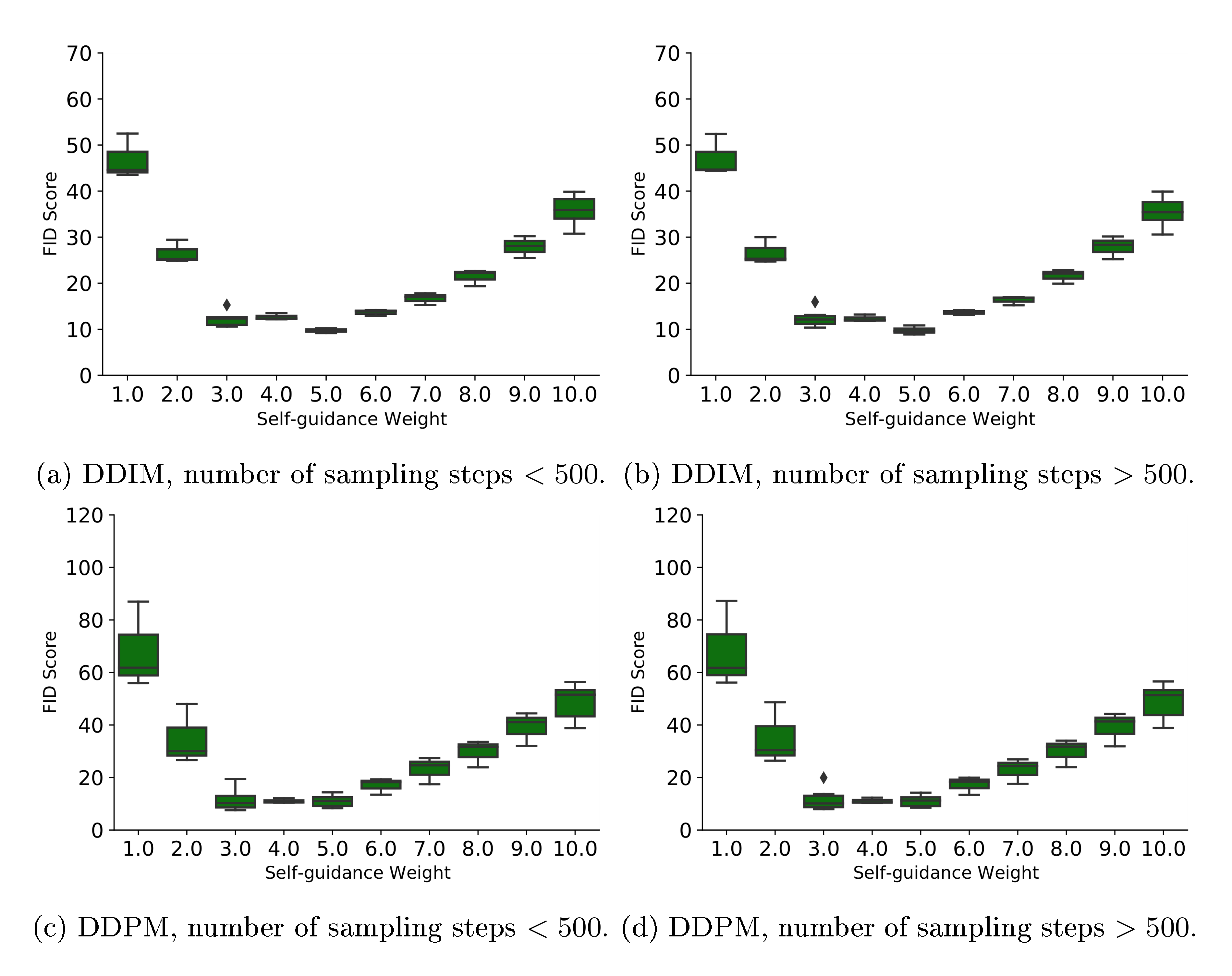
Self-Guidance	$5.15$	$5.65$	$\mathbf{7.87}$

Figure 12 shows FIDs on conditional $\textsc{ImageNet 64 $ \times $ 64}$ with $\textsc{uint8}$ encoding, using Momentum Estimate with different sampling steps. We find that the momentum on the data estimate is only helpful when sampling steps are larger.

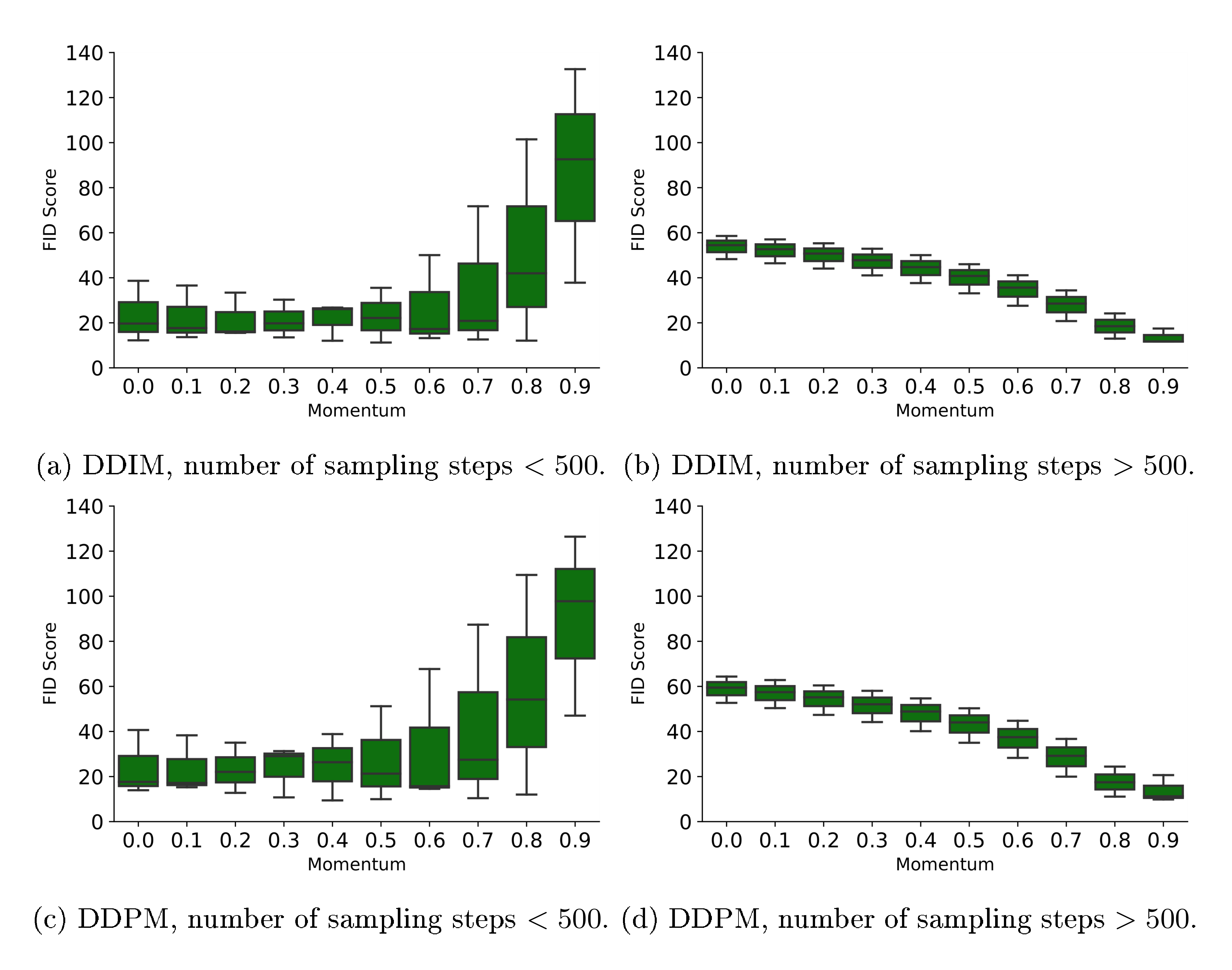
Figure 13 shows FIDs on conditional $\textsc{ImageNet 64 $ \times $ 64}$ with $\textsc{uint8}$ encoding, using Self-Guidance with different sampling steps. We find that a guidance weight between 3.0 and 5.0 is generally preferable and robust to other hyper-parameters (such as sampler choice, sampling steps, and time difference).

G.3 Samples

Figure 14 and 15 provide generated samples from different sampling strategies with 100 and 1000 DDIM sampling steps, respectively.

References

Section Summary: This references section lists about 30 key research papers and preprints from 2009 to 2022, focusing on advancements in artificial intelligence for generating images, text, and sequences. It covers early works on neural networks for image creation, like PixelCNN, and influential ideas such as transformers and attention mechanisms that power modern language models. Later entries highlight diffusion models and score-based techniques, which have improved photorealistic image synthesis from text descriptions, drawing from datasets like ImageNet and contributions by researchers at organizations like OpenAI and Google.

[1] Aaron Van den Oord, Nal Kalchbrenner, Lasse Espeholt, Oriol Vinyals, Alex Graves, et al. Conditional image generation with pixelcnn decoders. Advances in neural information processing systems, 29, 2016.

[2] Tim Salimans, Andrej Karpathy, Xi Chen, and Diederik P Kingma. Pixelcnn++: Improving the pixelcnn with discretized logistic mixture likelihood and other modifications. arXiv preprint arXiv:1701.05517, 2017.

[3] Niki Parmar, Ashish Vaswani, Jakob Uszkoreit, Lukasz Kaiser, Noam Shazeer, Alexander Ku, and Dustin Tran. Image transformer. In International conference on machine learning, pp.\ 4055–4064. PMLR, 2018.

[4] Rewon Child, Scott Gray, Alec Radford, and Ilya Sutskever. Generating long sequences with sparse transformers. arXiv preprint arXiv:1904.10509, 2019.

[5] Aurko Roy, Mohammad Saffar, Ashish Vaswani, and David Grangier. Efficient content-based sparse attention with routing transformers. Transactions of the Association for Computational Linguistics, 9:53–68, 2021.

[6] Heewoo Jun, Rewon Child, Mark Chen, John Schulman, Aditya Ramesh, Alec Radford, and Ilya Sutskever. Distribution augmentation for generative modeling. In International Conference on Machine Learning, pp.\ 5006–5019. PMLR, 2020.

[7] Ilya Sutskever, Oriol Vinyals, and Quoc V Le. Sequence to sequence learning with neural networks. Advances in neural information processing systems, 27, 2014.

[8] Tom Brown, Benjamin Mann, Nick Ryder, Melanie Subbiah, Jared D Kaplan, Prafulla Dhariwal, Arvind Neelakantan, Pranav Shyam, Girish Sastry, Amanda Askell, et al. Language models are few-shot learners. Advances in neural information processing systems, 33:1877–1901, 2020.

[9] Aakanksha Chowdhery, Sharan Narang, Jacob Devlin, Maarten Bosma, Gaurav Mishra, Adam Roberts, Paul Barham, Hyung Won Chung, Charles Sutton, Sebastian Gehrmann, et al. Palm: Scaling language modeling with pathways. arXiv preprint arXiv:2204.02311, 2022.

[10] Ashish Vaswani, Noam Shazeer, Niki Parmar, Jakob Uszkoreit, Llion Jones, Aidan N Gomez, Łukasz Kaiser, and Illia Polosukhin. Attention is all you need. Advances in neural information processing systems, 30, 2017.

[11] Jascha Sohl-Dickstein, Eric Weiss, Niru Maheswaranathan, and Surya Ganguli. Deep unsupervised learning using nonequilibrium thermodynamics. In International Conference on Machine Learning, pp.\ 2256–2265. PMLR, 2015.

[12] Jonathan Ho, Ajay Jain, and Pieter Abbeel. Denoising diffusion probabilistic models. Advances in Neural Information Processing Systems, 33:6840–6851, 2020.

[13] Jiaming Song, Chenlin Meng, and Stefano Ermon. Denoising diffusion implicit models. arXiv preprint arXiv:2010.02502, 2020.

[14] Yang Song and Stefano Ermon. Generative modeling by estimating gradients of the data distribution. Advances in Neural Information Processing Systems, 32, 2019.

[15] Yang Song and Stefano Ermon. Improved techniques for training score-based generative models. Advances in neural information processing systems, 33:12438–12448, 2020.

[16] Yang Song, Jascha Sohl-Dickstein, Diederik P Kingma, Abhishek Kumar, Stefano Ermon, and Ben Poole. Score-based generative modeling through stochastic differential equations. In International Conference on Learning Representations, 2021.

[17] Prafulla Dhariwal and Alexander Nichol. Diffusion models beat gans on image synthesis. Advances in Neural Information Processing Systems, 34:8780–8794, 2021.

[18] Jonathan Ho, Chitwan Saharia, William Chan, David J Fleet, Mohammad Norouzi, and Tim Salimans. Cascaded diffusion models for high fidelity image generation. J. Mach. Learn. Res., 23:47–1, 2022.

[19] Alex Nichol, Prafulla Dhariwal, Aditya Ramesh, Pranav Shyam, Pamela Mishkin, Bob McGrew, Ilya Sutskever, and Mark Chen. Glide: Towards photorealistic image generation and editing with text-guided diffusion models. arXiv preprint arXiv:2112.10741, 2021.

[20] Aditya Ramesh, Prafulla Dhariwal, Alex Nichol, Casey Chu, and Mark Chen. Hierarchical text-conditional image generation with clip latents. arXiv preprint arXiv:2204.06125, 2022.

[21] Chitwan Saharia, William Chan, Saurabh Saxena, Lala Li, Jay Whang, Emily Denton, Seyed Kamyar Seyed Ghasemipour, Burcu Karagol Ayan, S Sara Mahdavi, Rapha Gontijo Lopes, et al. Photorealistic text-to-image diffusion models with deep language understanding. arXiv preprint arXiv:2205.11487, 2022.

[22] Emiel Hoogeboom, Didrik Nielsen, Priyank Jaini, Patrick Forré, and Max Welling. Argmax flows and multinomial diffusion: Learning categorical distributions. Advances in Neural Information Processing Systems, 34:12454–12465, 2021.

[23] Jacob Austin, Daniel D Johnson, Jonathan Ho, Daniel Tarlow, and Rianne van den Berg. Structured denoising diffusion models in discrete state-spaces. Advances in Neural Information Processing Systems, 34:17981–17993, 2021.

[24] Alexander Quinn Nichol and Prafulla Dhariwal. Improved denoising diffusion probabilistic models. In International Conference on Machine Learning, pp.\ 8162–8171. PMLR, 2021.

[25] Chitwan Saharia, Jonathan Ho, William Chan, Tim Salimans, David J Fleet, and Mohammad Norouzi. Image super-resolution via iterative refinement. arXiv preprint arXiv:2104.07636, 2021.

[26] Alex Krizhevsky, Geoffrey Hinton, et al. Learning multiple layers of features from tiny images. 2009.

[27] Jia Deng, Wei Dong, Richard Socher, Li-Jia Li, Kai Li, and Li Fei-Fei. Imagenet: A large-scale hierarchical image database. In 2009 IEEE conference on computer vision and pattern recognition, pp.\ 248–255. Ieee, 2009.

[28] Martin Heusel, Hubert Ramsauer, Thomas Unterthiner, Bernhard Nessler, and Sepp Hochreiter. Gans trained by a two time-scale update rule converge to a local nash equilibrium. Advances in neural information processing systems, 30, 2017.

[29] Ting Chen, Saurabh Saxena, Lala Li, Tsung-Yi Lin, David J Fleet, and Geoffrey Hinton. A unified sequence interface for vision tasks. arXiv preprint arXiv:2206.07669, 2022.

[30] Tsung-Yi Lin, Michael Maire, Serge Belongie, James Hays, Pietro Perona, Deva Ramanan, Piotr Dollár, and C Lawrence Zitnick. Microsoft coco: Common objects in context. In European Conference on Computer Vision, pp.\ 740–755. Springer, 2014.

[31] Andrew Brock, Jeff Donahue, and Karen Simonyan. Large scale gan training for high fidelity natural image synthesis. arXiv preprint arXiv:1809.11096, 2018.

[32] Taku Kudo and John Richardson. Sentencepiece: A simple and language independent subword tokenizer and detokenizer for neural text processing. arXiv preprint arXiv:1808.06226, 2018.

[33] Olaf Ronneberger, Philipp Fischer, and Thomas Brox. U-net: Convolutional networks for biomedical image segmentation. In International Conference on Medical image computing and computer-assisted intervention, pp.\ 234–241. Springer, 2015.

[34] Kaiming He, Xiangyu Zhang, Shaoqing Ren, and Jian Sun. Deep residual learning for image recognition. In Proceedings of the IEEE conference on computer vision and pattern recognition, pp.\ 770–778, 2016.

[35] Nitish Srivastava, Geoffrey Hinton, Alex Krizhevsky, Ilya Sutskever, and Ruslan Salakhutdinov. Dropout: a simple way to prevent neural networks from overfitting. The journal of machine learning research, 15(1):1929–1958, 2014.

[36] Ting Chen, Saurabh Saxena, Lala Li, David J Fleet, and Geoffrey Hinton. Pix2seq: A language modeling framework for object detection. arXiv preprint arXiv:2109.10852, 2021.

[37] Diederik P Kingma and Jimmy Ba. Adam: A method for stochastic optimization. arXiv preprint arXiv:1412.6980, 2014.

[38] Andrew Campbell, Joe Benton, Valentin De Bortoli, Tom Rainforth, George Deligiannidis, and Arnaud Doucet. A continuous time framework for discrete denoising models. arXiv preprint arXiv:2205.14987, 2022.

[39] Mark Chen, Alec Radford, Rewon Child, Jeffrey Wu, Heewoo Jun, David Luan, and Ilya Sutskever. Generative pretraining from pixels. In International conference on machine learning, pp.\ 1691–1703. PMLR, 2020a.

[40] Xiang Lisa Li, John Thickstun, Ishaan Gulrajani, Percy Liang, and Tatsunori B Hashimoto. Diffusion-lm improves controllable text generation. arXiv preprint arXiv:2205.14217, 2022.

[41] Danilo Rezende and Shakir Mohamed. Variational inference with normalizing flows. In International conference on machine learning, pp.\ 1530–1538. PMLR, 2015.

[42] Laurent Dinh, Jascha Sohl-Dickstein, and Samy Bengio. Density estimation using real NVP. In International Conference on Learning Representations, 2017.

[43] Durk P Kingma and Prafulla Dhariwal. Glow: Generative flow with invertible 1x1 convolutions. Advances in neural information processing systems, 31, 2018.

[44] Dustin Tran, Keyon Vafa, Kumar Agrawal, Laurent Dinh, and Ben Poole. Discrete flows: Invertible generative models of discrete data. Advances in Neural Information Processing Systems, 32, 2019.

[45] Emiel Hoogeboom, Jorn Peters, Rianne Van Den Berg, and Max Welling. Integer discrete flows and lossless compression. Advances in Neural Information Processing Systems, 32, 2019.

[46] Alexandra Lindt and Emiel Hoogeboom. Discrete denoising flows. arXiv preprint arXiv:2107.11625, 2021.

[47] Phillip Lippe and Efstratios Gavves. Categorical normalizing flows via continuous transformations. In International Conference on Learning Representations, 2021.

[48] Shawn Tan, Chin-Wei Huang, Alessandro Sordoni, and Aaron Courville. Learning to dequantise with truncated flows. In International Conference on Learning Representations, 2021.

[49] Lucas Theis, Aäron van den Oord, and Matthias Bethge. A note on the evaluation of generative models. arXiv preprint arXiv:1511.01844, 2015.

[50] Durk P Kingma, Tim Salimans, Rafal Jozefowicz, Xi Chen, Ilya Sutskever, and Max Welling. Improved variational inference with inverse autoregressive flow. Advances in neural information processing systems, 29, 2016.

[51] Zachary Ziegler and Alexander Rush. Latent normalizing flows for discrete sequences. In International Conference on Machine Learning, pp.\ 7673–7682. PMLR, 2019.

[52] Zijun Zhang, Ruixiang Zhang, Zongpeng Li, Yoshua Bengio, and Liam Paull. Perceptual generative autoencoders. In International Conference on Machine Learning, pp.\ 11298–11306. PMLR, 2020.

[53] Diederik P Kingma and Max Welling. Auto-encoding variational bayes. arXiv preprint arXiv:1312.6114, 2013.

[54] Ian Goodfellow, Jean Pouget-Abadie, Mehdi Mirza, Bing Xu, David Warde-Farley, Sherjil Ozair, Aaron Courville, and Yoshua Bengio. Generative adversarial nets. Advances in neural information processing systems, 27, 2014.

[55] Lantao Yu, Weinan Zhang, Jun Wang, and Yong Yu. Seqgan: Sequence generative adversarial nets with policy gradient. In Proceedings of the AAAI conference on artificial intelligence, volume 31, 2017.

[56] Tong Che, Yanran Li, Ruixiang Zhang, R Devon Hjelm, Wenjie Li, Yangqiu Song, and Yoshua Bengio. Maximum-likelihood augmented discrete generative adversarial networks. arXiv preprint arXiv:1702.07983, 2017.

[57] R Devon Hjelm, Athul Paul Jacob, Tong Che, Adam Trischler, Kyunghyun Cho, and Yoshua Bengio. Boundary-seeking generative adversarial networks. arXiv preprint arXiv:1702.08431, 2017.

[58] William Fedus, Ian Goodfellow, and Andrew M Dai. Maskgan: better text generation via filling in the_. arXiv preprint arXiv:1801.07736, 2018.

[59] Ting Chen, Mario Lucic, Neil Houlsby, and Sylvain Gelly. On self modulation for generative adversarial networks. arXiv preprint arXiv:1810.01365, 2018a.

[60] Nikolay Savinov, Junyoung Chung, Mikolaj Binkowski, Erich Elsen, and Aaron van den Oord. Step-unrolled denoising autoencoders for text generation. arXiv preprint arXiv:2112.06749, 2021.

[61] Rico Sennrich, Barry Haddow, and Alexandra Birch. Neural machine translation of rare words with subword units. arXiv preprint arXiv:1508.07909, 2015.

[62] Ting Chen, Martin Renqiang Min, and Yizhou Sun. Learning k-way d-dimensional discrete codes for compact embedding representations. In International Conference on Machine Learning, pp.\ 854–863. PMLR, 2018b.

[63] Ting Chen, Lala Li, and Yizhou Sun. Differentiable product quantization for end-to-end embedding compression. In International Conference on Machine Learning, pp.\ 1617–1626. PMLR, 2020b.

[64] Cheng Lu, Yuhao Zhou, Fan Bao, Jianfei Chen, Chongxuan Li, and Jun Zhu. Dpm-solver: A fast ode solver for diffusion probabilistic model sampling in around 10 steps. arXiv preprint arXiv:2206.00927, 2022.

[65] Jonathan Ho and Tim Salimans. Classifier-free diffusion guidance. In NeurIPS 2021 Workshop on Deep Generative Models and Downstream Applications, 2021.