
Superposition Yields Robust Neural Scaling
Yizhou Liu, Ziming Liu, and Jeff Gore
Massachusetts Institute of Technology
liuyz, zmliu, [email protected]
Abstract
The success of today's large language models (LLMs) depends on the observation that larger models perform better. However, the origin of this neural scaling law, that loss decreases as a power law with model size, remains unclear. We propose that representation superposition, meaning that LLMs represent more features than they have dimensions, can be a key contributor to loss and cause neural scaling. Based on Anthropic's toy model, we use weight decay to control the degree of superposition, allowing us to systematically study how loss scales with model size. When superposition is weak, the loss follows a power law only if data feature frequencies are power-law distributed. In contrast, under strong superposition, the loss generically scales inversely with model dimension across a broad class of frequency distributions, due to geometric overlaps between representation vectors. We confirmed that open-sourced LLMs operate in the strong superposition regime and have loss scaling inversely with model dimension, and that the Chinchilla scaling laws are also consistent with this behavior. Our results identify representation superposition as a central driver of neural scaling laws, providing insights into questions like when neural scaling laws can be improved and when they will break down.[^1]
[^1]: Code is available at https://github.com/liuyz0/SuperpositionScaling
Executive Summary: Superposition in neural networks—representing more features than model dimensions allow—explains much of the observed neural scaling behavior in large language models.
Large language models achieve better performance as they grow in size, with loss typically decreasing as a power law in model dimension. The origin of this reliable pattern has remained unclear, as prior theoretical accounts often assume conditions unlike those in actual LLMs and do not fully account for how models embed far more tokens and concepts than their width permits.
This paper set out to test whether representation superposition drives scaling laws. The authors asked specifically when loss scales as a power law with model width and what the scaling exponent should be under different degrees of superposition and data structures.
They used a simplified autoencoder toy model adapted from prior work, in which input features occur with controllable frequencies and a weight-decay term tunes the degree of superposition. Experiments scanned model widths from 10 to 100 (plus larger confirmatory runs), multiple feature-frequency distributions, and a wide range of weight-decay values. They then compared the resulting scaling behavior to weight matrices and evaluation losses from four families of open-source LLMs spanning roughly 100 M to 70 B parameters.
In the weak-superposition regime, loss equals the total frequency of unrepresented features; a power-law decay with width therefore appears only when feature frequencies themselves follow a power law. In the strong-superposition regime, loss arises from geometric overlaps among representation vectors; these overlaps produce a robust loss scaling of approximately 1/m across a broad class of frequency distributions. Open-source LLMs operate squarely in the strong-superposition regime: their token-representation overlaps scale as 1/m, token frequencies follow a power law with exponent near 1, and measured loss that depends on model size scales with an exponent of roughly 0.9—matching both the toy-model prediction and the Chinchilla scaling laws after conversion from parameter count to width.
These results indicate that superposition is a central mechanism behind the near-universal width scaling observed in practice. Because the scaling arises from geometry rather than data statistics alone, it is difficult to improve upon by ordinary architectural changes, yet it should eventually saturate once width approaches the effective number of independent features in language. The same geometry also suggests that deliberate encouragement of superposition could allow smaller models to reach performance previously requiring larger ones.
The analysis rests on a highly abstracted toy model and correlational checks on existing LLMs; causal confirmation would require controlled interventions in full-scale training. Within these bounds the findings are consistent across regimes and model families.
Practitioners should therefore treat 1/m scaling as the expected baseline rather than an accident of current data or architectures. Future work should quantify how much of total loss is representation-limited versus processing-limited, test whether optimizers or constraints that favor superposition measurably improve efficiency, and examine whether highly skewed domain data can produce faster-than-1/m scaling.
1. Introduction
Section Summary: The introduction explains that large language models get better as they grow in size according to simple power-law patterns, but the reason for this steady improvement with model width remains unclear. It highlights how superposition—fitting more features into a limited-dimensional space by allowing overlap—may be key, especially in the strong-overlap regime used by actual LLMs, and shows through a toy model that this regime produces robust “one-over-width” loss scaling regardless of data details. The work contrasts this with weaker superposition cases and notes that real LLMs match the strong-superposition predictions quantitatively.
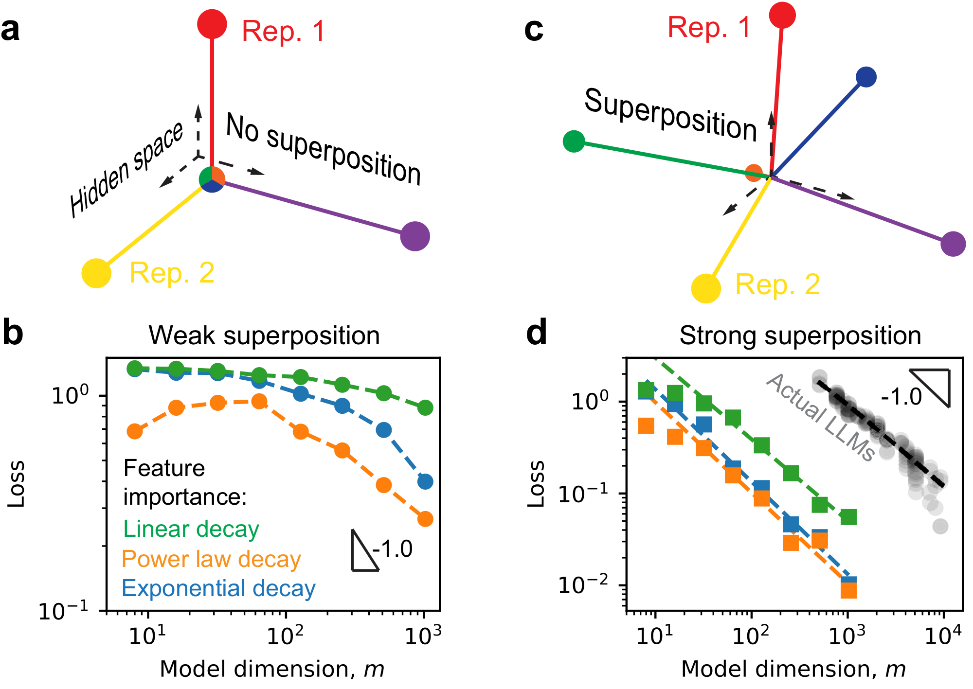
The remarkable success of large language models (LLMs) has been driven by the empirical observation that increasing model size, training data, and compute consistently leads to better performance [1, 2, 3, 4]. Across a wide range of tasks — including language understanding [1, 5, 6], math [7, 8, 9, 10], and code generation [11, 12] — larger models achieve lower loss, higher accuracy, and greater generalization abilities [2, 13]. This consistent trend, known as neural scaling laws, has been observed across multiple model families and architectures, fueling the development of increasingly large models [2, 3, 4]. These scaling laws have not only shaped the current strategies for building better models but have also raised fundamental questions about why such simple and universal patterns emerge in complex learning systems.
The power-law loss with model size plays a central role in both the practical design and the theoretical understanding of large-scale machine learning systems, yet its origin remains inconclusive [3, 14, 15, 16, 17, 18, 19, 20, 21, 22, 23, 24, 25]. Various explanations have been proposed, drawing from statistical learning theory and empirical phenomenological models, including improved function or manifold approximation in larger models [14, 15], and enhanced representation or skill learning in larger models [19, 20, 21, 22]. In the limit of infinite data, many of these explanations predict a power-law decay of loss with model size, provided the underlying data distribution also follows a power law. The scaling exponents are sensitive to the properties of the data distribution. Moreover, the connection between these mechanistic explanations and the behavior of actual LLMs needs further exploration.
When considering LLMs specifically, it becomes clear that representation or embedding can be a limiting factor, which is closely related to a phenomenon called superposition [26, 27], yet this aspect has not been thoroughly studied. LLMs must learn embedding vectors for tokens, process these representations through transformer layers to predict the next token, and use a final projection (the language model head) to generate the output. Conceptually, fitting functions or manifolds and learning skills or grammars are primarily tasks of the transformer layers, while representation is more directly tied to the embedding matrix and the language model head. To represent more than fifty thousand tokens — or even more abstract concepts — within a hidden space of at most a few thousand dimensions, the quality of representations is inevitably constrained by the model dimension or width, contributing to the final loss. Although models can represent more features than their dimensionality would suggest through a mechanism known as superposition [27], prior works on neural scaling laws seem to fall in the weak superposition regime implicitly [15, 16, 17, 18, 19, 20], which may be less relevant to the regime where LLMs operate. This gap leads us to study
Varying the degree of superposition and data structure, when is the loss a power law? And if the loss is a power law, what will the exponent be?
We adopt a toy model construction similar to [27] to study how superposition affects neural scaling laws. In the toy model, representations are learned by recovering data, each composed of multiple latent features. These features in data have different frequencies of occurrence, reflecting their relative importance. Weak superposition means that only the most frequent features are perfectly represented, while the others are ignored. As illustrated in Figure 1 a, the first three of six features are represented in the three-dimensional space without interference, and the remaining three are omitted. We find that in the weak superposition regime, the scaling of loss with model dimension depends sensitively on how feature frequency decays with rank: the loss follows a power law with model size only if the feature frequencies themselves follow a power law, provided that $m$ is sufficiently large (Figure 1 b). By contrast, strong superposition allows many more features to be represented, albeit with overlap in the representation (Figure 1 c). In this regime, the model displays a robust behavior: loss scales inversely with model dimension across different data frequency distributions (Figure 1 d). Remarkably, we find that actual LLMs follow a similar scaling. We summarize our contributions as
$\bullet$ Loss in the weak superposition regime depends on summing frequencies of ignored features, which is a power law if frequencies follow a power law.

$\bullet$ In the strong superposition regime, loss arises from the interference between representations and can have robust "one over width" scaling because of the geometry.

$\bullet$ LLMs exhibit strong superposition and agree quantitatively with our toy model predictions.
The rest of the paper will elaborate on the takeaways. In Section 2, we introduce the toy model, describe the data sampling procedure, and explain how we control the degree of superposition. Section 3 presents the detailed results. In Section 4, we compare our findings to related works. Finally, Section 5 summarizes our conclusions and discusses limitations and future directions.
2. Methods
Section Summary: The authors employ a simplified autoencoder toy model to investigate superposition, where input data consists of n sparse features (with varying activation frequencies p_i drawn from a Bernoulli-uniform distribution) that must be represented in a much smaller hidden dimension m. The model embeds each input via a weight matrix W into this bottleneck space and reconstructs it using a ReLU nonlinearity and bias, with training loss defined as the mean squared reconstruction error; superposition arises when more than m features end up with nonzero rows in W despite the dimensionality constraint. To control the strength of superposition, the authors add a tunable decoupled weight decay term (positive or negative) that encourages either sparse or uniform-norm representations in W.
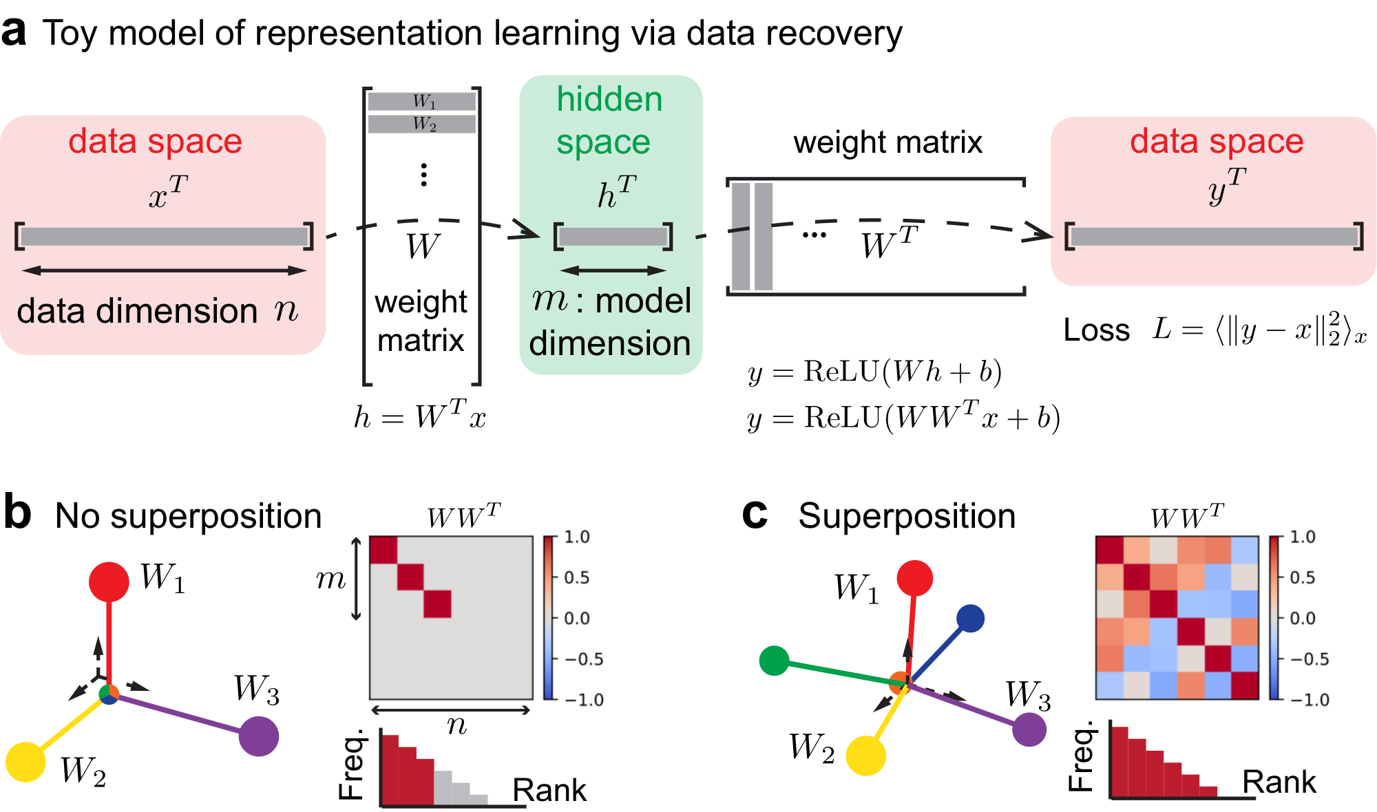
To understand the relationship between superposition and data structure, we need a toy model to represent data features simple enough yet not simpler — two key principles need to be reflected, (i) there are more features to represent than the dimension of the model, and (ii) features occur in data with different frequencies. Later, we will discuss how the loss due to representation studied here may affect the overall final loss in LLMs.
We adopt the toy model of superposition from Anthropic [27] (an autoencoder) with minor modifications (Figure 2 a). Input $x \in \mathbb{R}^n$ is a vector with data dimension $n$ being the number of atomic (or irreducible) features. Each element $x_i$ in $x$ is interpreted as the activation of this sample at feature $i$, which follows
$
x_i = u_i v_i, u_i \sim Bernoulli(p_i)&~v_i\sim U(0, 2).\tag{1}
$
Here, $u_i$ sampled from a Bernoulli distribution controls whether the feature $i$ is activated, and $v_i$ sampled from a uniform distribution controls the activation strength once feature $i$ is activated. All samples are i.i.d. The frequency of feature $i$ to appear in the data is $p_i$. Without loss of generality, we make the indices of features the same as their frequency or importance rank. The data structure is then about how $p_i$ decreases with rank $i$. The expected number of activations in one input will be referred to as activation density: $E = \sum_{i=1}^n p_i$. The model learns hidden representations by recovering the data, which cannot be done perfectly because the model dimension $m$ is much smaller than the number of possible features in the data $n$. The trainable parameters are a weight matrix $W \in \mathbb{R}^{n\times m}$ and a bias vector $b\in \mathbb{R}^{n}$. The weight matrix embeds data $x$ into a hidden space with dimension $m$, $h = W^T x$, with $m\ll n$. In practice, we fix $n$ as a large number and change the model dimension $m$. We use $W$ to read out the embedding, where $y = \mathrm{ReLU}(Wh + b)$. The loss is defined as the difference between the recovered $y$ and the original $x$, $L = \langle |y - x|_2^2 \rangle_x$, where $\langle \cdot \rangle_x$ means average over $x$ distribution.
We can now formally introduce superposition. Note that $W_i$ is the representation of feature $i$ in the hidden space, where we use $W_i$ to denote the $i$ th row of the $W$ matrix. We emphasize the following
$\bullet$ Feature frequency: $p_i$ is the probability that feature $i$ is activated (non-zero) in a sample, which is assumed to decrease with $i$.

$\bullet$ Sparsity: We say features are sparse when $E / n$ is small.

$\bullet$ The feature $i$ is represented (in the hidden space) when $W_i$ is non-zero.
No superposition ideally means the first $m$ rows of $W$ form an orthogonal basis (i.e., the first $m$ most important features represented perfectly) and the rest of the rows are zero (i.e., the rest of the features ignored or lost), as illustrated in Figure 2 b. Superposition means that there are more than $m$ rows in $W$ with non-zero norms (Figure 2 c).
We next summarize important facts of this toy model [27]:
Superposition cannot lead to lower losses in a linear model (without ReLU function) due to the large amount of interference. ReLU and negative biases can cancel off interference, realizing error correction. With this non-linearity, superposition can be preferred when feature frequencies are more even (better not to ignore features) and features are sparse in data (error correction is easier).
We can see that in Figure 1, where features are sparse in data, the losses in the strong superposition regime are indeed much smaller than those in the weak superposition regime across several feature frequency distributions.
If one regime is more preferred, we want to approach it more quickly in training. If it is not preferred, we also want to study the scaling behaviors scientifically in that regime. To this end, we introduce a decoupled weight decay (or growth) term in training to tune the degree of superposition:
$ W_{i, t+1} = \left{ \begin{aligned} &W_{i, t} - \eta_t \gamma W_{i, t}, ~ \gamma \geq 0, \ &W_{i, t} - \eta_t \gamma W_{i, t} (1 / | W_{i, t} |_2 - 1), ~ \gamma < 0, \end{aligned} \right.\tag{2} $
where $\eta_t$ is the learning rate and $W{i, t}$ is the $i$ th row of the weight matrix at step $t$ (vector operations are element-wise). For weight decay $\gamma < 0$, the update corresponds to gradient descent on $(|W_{i, t}|_2 - 1)^2$, encouraging unit-norm rows. We implement this weight decay in AdamW [28] optimizer with a warm-up and cosine decay learning rate schedule (details in Appendix B). At each training step, we sample new data.
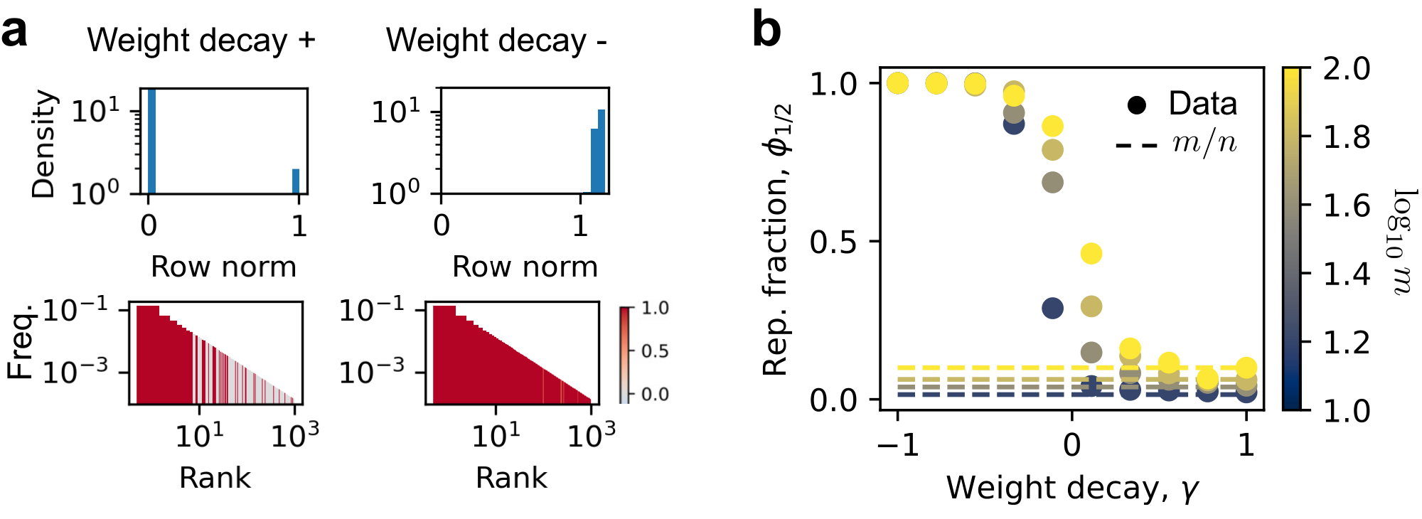
We find that the weight decay can robustly control superposition. We first see that important features tend to be represented (associated $|W_i|_2>0$), and norms of $W_i$ become bimodal, clustering near 0 or 1 (Figure 3 a). This allows us to define the fraction of represented features as
$ \phi_{1/2} = |{ i : |W_i |_2 > 1/2 }| / n,\tag{3} $
namely, the fraction of rows with norm larger than $1/2$.[^2] We found that weight decay can tune superposition for all models we trained, with small weight decay $\gamma$ giving strong superposition, i.e., $\phi_{1/2} \approx 1 \gg m/n$, and large weight decay corresponding to weak superposition, i.e., $\phi_{1/2} \sim m/n$ (Figure 3 b). The ability of weight decay to tune superposition is robust to feature frequency distributions (Appendix D.3). We can then systematically study scaling behaviors in different regimes.
[^2]: In theory, we should use $0$ as the threshold. The choice, $1/2$, may minimize misclassifications since norms are near $0$ or $1$. Our result is robust to this threshold since norms are very concentrated.
The toy model differs from LLMs in architecture, data, and loss. Since we focus on representations rather than next-token prediction, we omit transformer layers. Conceptually, LLMs map a document to a token, with inputs and outputs in different spaces, while the toy model operates within a single shared space. Despite this, the toy model captures key aspects of language structure through engineered sparsity and feature importance, making its data structure aligned with that of LLMs at a high level. While LLMs use cross-entropy loss and the toy model uses squared error, we can show that this does not affect the scaling behaviors (Appendix A.2). Thus, the toy model is a suitable abstraction for studying representation-limited scaling.
3. Results
Section Summary: The results analyze loss scaling with model size when learning features whose importance follows a power-law frequency distribution. In the weak superposition regime, the model perfectly encodes the most frequent features up to its capacity, so loss is governed by the summed frequencies of the remaining features and therefore declines as a power law whose exponent is determined by the input distribution. In the strong superposition regime, feature representations overlap and the resulting interference produces different power-law exponents, which are explained by the geometry of roughly isotropic vectors when frequencies are flat and by structured norms and overlaps when frequencies are highly skewed.
For a systematic scan, we set $p_i \propto 1/i^\alpha $ in this section and can vary the data exponent $\alpha$ to change how skewed $p_i$ is.[^3] The activation density $E$ is set as $1$, whose value can be shown to not affect the scaling (Appendix D.4). We fix data dimension $n = 1000$, vary model dimension $m$ from $10$ to $100$, and sweep weight decay $\gamma$ from $-1$ to $1$. We fit final test losses as a power law, $L \propto 1 / m^{\alpha_m}$, and call $\alpha_m$ the model exponent. More details on hyperparameters are in Appendix B.2.
[^3]: The word or phrase frequency in natural language follows Zipf's law, which is a power law ($\alpha = 1$).
3.1 Weak superposition
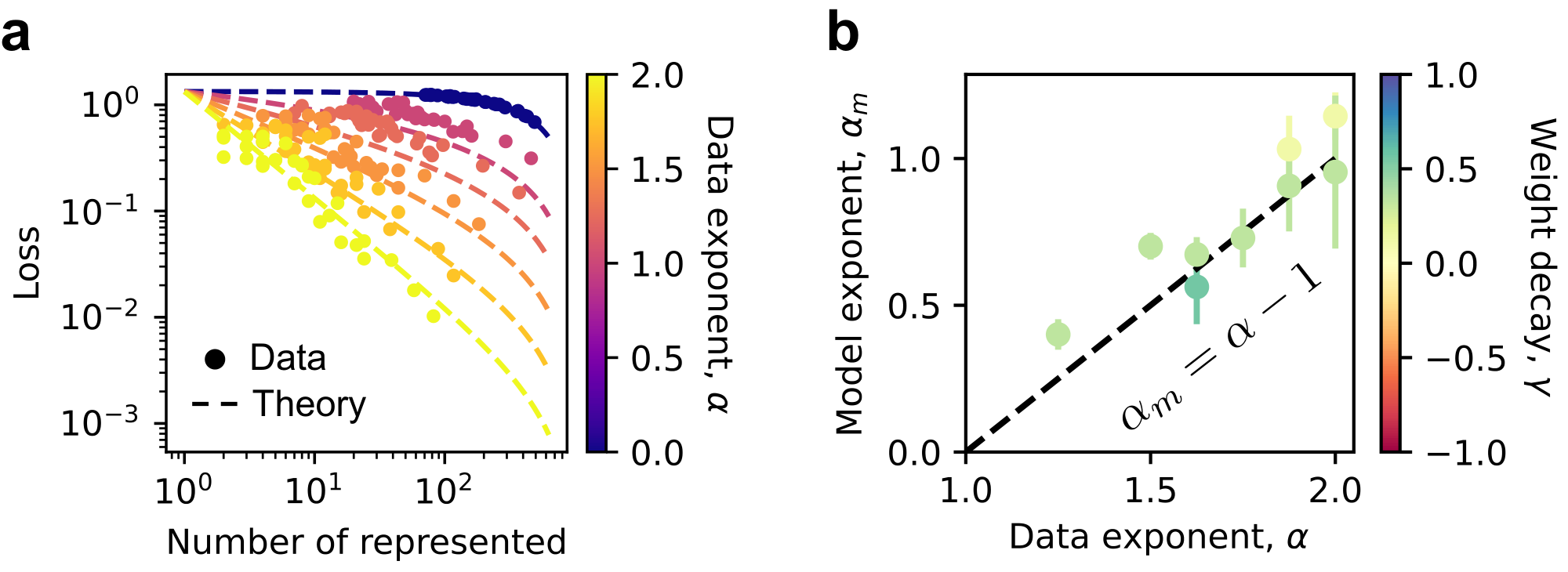
We seek to understand when loss follows a power law with model dimension, and what determines the exponent when it does in the weak superposition regime. Consider an idealized case where the top $\phi_{1/2} n$ most frequent features are perfectly represented (no overlap), where $\phi_{1/2}$ is the fraction of represented features. The optimal biases are $b_i = 0$ for $i\leq \phi_{1/2} n$ and $b_i = \langle x_i \rangle$ for $i > \phi_{1/2} n$ [27]. The loss can then be written as:
$ L = \sum_{i>\phi_{1/2} n} \langle (x_i - \langle x_i \rangle)^2 \rangle = \sum_{i>\phi_{1/2} n} (\langle v^2 \rangle p_i -\langle v \rangle^2 p_i^2) \approx \langle v^2 \rangle \sum_{i>\phi_{1/2} n} p_i.\tag{4} $
The last approximation is right when $p_i \ll 1$ for $i>\phi_{1/2} n$ and $p_i^2$ terms are negligible. We use the definition of $x_i = u_i v_i$, where $v \sim U(0, 2)$, giving $\langle v^2 \rangle = 4/3$. We can use the integral $\int_{\phi_{1/2} n}^n p_i \mathrm{d}i$ to estimate the summation, yielding an expression that depends on the number of represented, $\phi_{1/2} n$, and the data exponent, $\alpha$ (Appendix D.5). We find that, in the weak superposition regime, the actual losses closely match this prediction (Figure 4 a). Focusing on cases closest to the ideal no-superposition scenario, where $\phi_{1/2} n = m$ and the first $m$ features are represented, we observe that such cases occur when $\alpha > 1$ and yield a model exponent $\alpha_m \approx \alpha - 1$ (Figure 4 b). This matches the theoretical expectation that $\int_m^n p_i \mathrm{d}i \propto m^{-\alpha + 1}$ when $n \gg m$ and $\alpha > 1$. Thus, in the weak superposition regime, loss scaling is well described by the contribution of unlearned features, that is, the total frequency of features not represented by the model.
We can now answer our Question in the weak superposition regime.
The loss is governed by a sum of frequencies of less frequent and not represented features. Ideally, there are model dimension $m$ most important features being represented. If feature frequencies follow a power law, $p_i \propto 1/i^\alpha$ with $\alpha > 1$, the loss or the summation starting at $m$ will be a power law with $m$ with exponent $\alpha - 1$.
This finding of the specific toy model agrees with previous works with very different settings [15, 16, 17, 18, 19, 20], where some power-law skill importance or spectrum is assumed.
3.2 Strong superposition
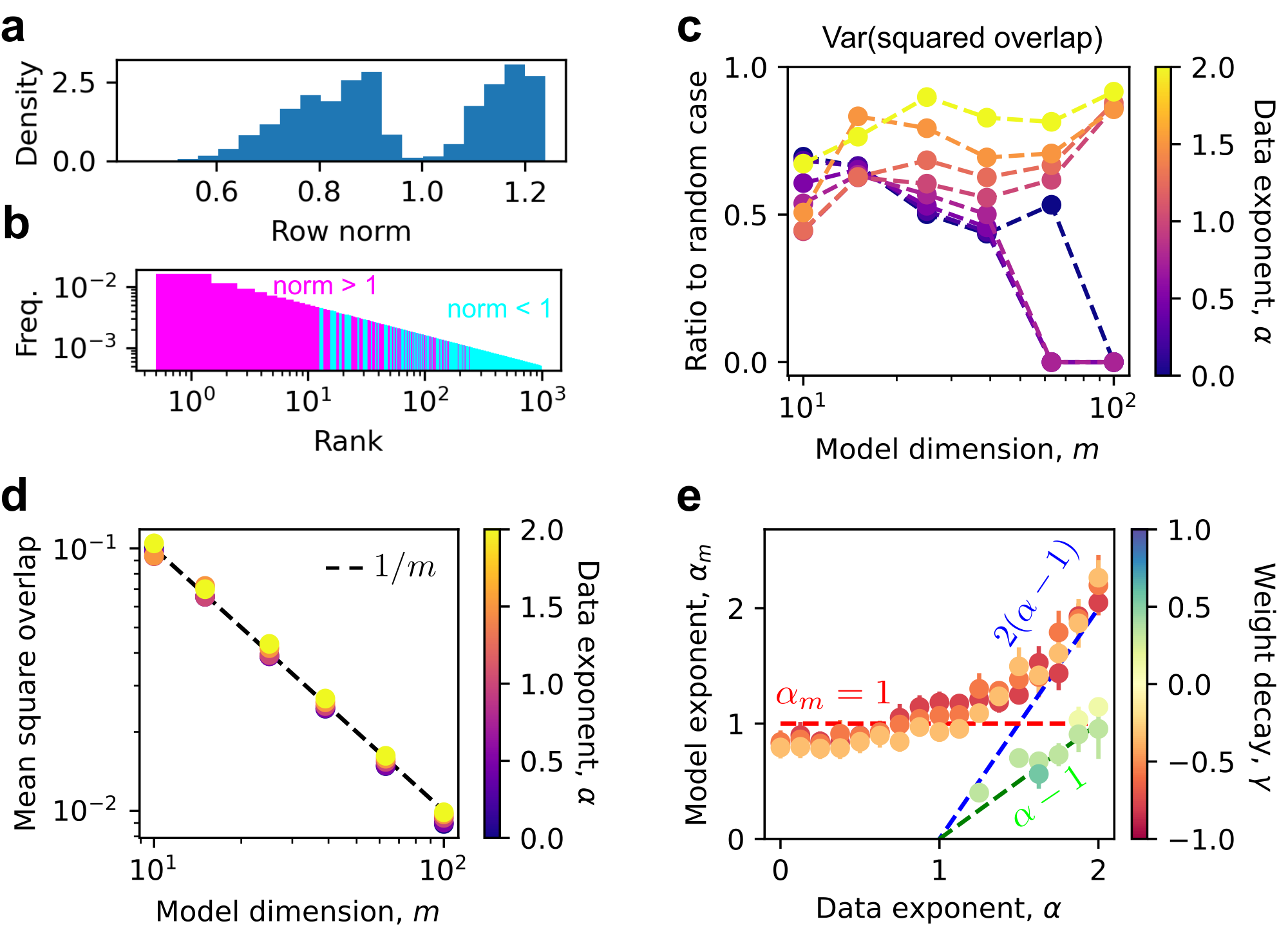
We next turn to the strong superposition regime. Consider the case where only feature $j$ is activated. The output $y_j$ has activation $\sim W_i \cdot W_j$, leading to a loss that scales as squared overlaps $(W_i \cdot W_j)^2$ due to the definition of loss. The loss arises from the non-zero overlaps between representation vectors. We cannot solve the weight matrix $W$ in this regime. The section goes back and forth between theoretical ansatz and experimental observations to understand the high-level behaviors.
We start by considering relatively even feature frequencies, where trained $W_i$ are expected to be isotropic. One simplest theoretical ansatz of isotropic vectors is i.i.d. vectors uniformly on the unit sphere. In $\mathbb{R}^m$, the squared overlap of two such random vectors follows $\mathrm{Beta}(\frac{1}{2}, \frac{m-1}{2})$ distribution, and therefore has mean $1/m$ and variance $\frac{2(m-1)}{m^2(m+2)} \sim 2/m^2$. The squared overlaps for isotropic random vectors typically obey $1/m$ scaling.
The actual trained $W_i$ have structures whose norms are bimodal near $1$ (Figure 5 a), and more important features tend to have larger vector norm (Figure 5 b). We want to understand how such a structure will change the scaling of overlaps. It turns out that for better error correction (using bias to cancel interference), the model needs to minimize the maximum overlap rather than the sum of squared overlaps. Consider $\nu$ unit vectors $w_i \in \mathbb{R}^m$ with $\nu \ge m$. It can be shown that [29]
$ \max_{i\neq j} | w_i \cdot w_j | \ge \sqrt{\frac{\nu - m}{m (\nu -1)}} \equiv \kappa. $
The lower bound, $\kappa \approx \sqrt{1/m}$ when $\nu \gg m$. The bound is met when the vectors form an equal angle tight frame (ETF) [30, 31, 32], which has no variance in absolute overlaps and appears in contexts such as quantum measurements [33, 34, 35, 36] and neural collapse [37, 38]. ETFs in real spaces can only exist if $\nu \le \frac{m(m+1)}{2}$ [30, 31, 32]. We find that the $W_i$ with $|W_i| > 1$ associated with important features tend to be ETF-like (Figure 5, c and d): the variance of squared overlaps is smaller than that of random vectors and can be near 0 for even feature frequencies (small $\alpha$); the mean of squared overlaps collapse on $1/m \approx \kappa^2$. Being ETF or ETF-like can help error correction and reduce loss values, but would not change the typical scaling with $m$ if the number of vectors is much larger than $m$. Similar to ETFs, whose number of vectors is bounded, the number of vectors $W_i$ with $|W_i| > 1$ is around $m^2/2$ (Appendix D.6), and the less important features tend not to be represented (norm lower than 1). Vectors of these less important features cannot be explained with a simple theoretical ansatz. Yet, combining the lessons from random vectors and ETF, we expect the squared overlaps to scale as $1/m$ robustly for isotropic vectors (confirmed in Appendix D.6). Considering all the overlaps when feature frequencies are even, we then predict the loss to scale as $1/m$, which is true (Figure 5 e).
When the feature frequencies are skewed (large $\alpha$), we find that the model exponent $\alpha_m$ increases with $\alpha$ and becomes greater than $1$. Vectors being non-isotropic, i.e., important features having much smaller overlaps, may lead to larger $\alpha_m$. To illustrate this idea, we conjecture an extreme situation where the $m^2/2$ most important features can be ETF-like and contribute negligible loss compared to the less important ones. In the worst case (Appendix A.1), the less important features lead to a loss proportional to $\sum_{i = m^2/2}^n p_i \sim m^{-2(\alpha -1)}$, i.e., $\alpha_m = 2(\alpha -1)$, which is close to observations (Figure 5 e). The real configuration of $W_i$ is more complicated than this simple conjecture, requiring advanced future studies on when $\alpha_m$ loses robustness and how it depends on feature frequencies sensitively then. To conclude the section, we have
For even feature frequencies, vectors $W_i$ tend to be isotropic in space with squared overlaps scaling like $1/m$ when $n\gg m$, leading to the robust $1/m$ power-law loss. For skewed feature frequencies, representation vectors are heterogeneous in space, making loss sensitive to feature frequencies, where it might need power-law frequencies to have power-law losses.
3.3 LLMs
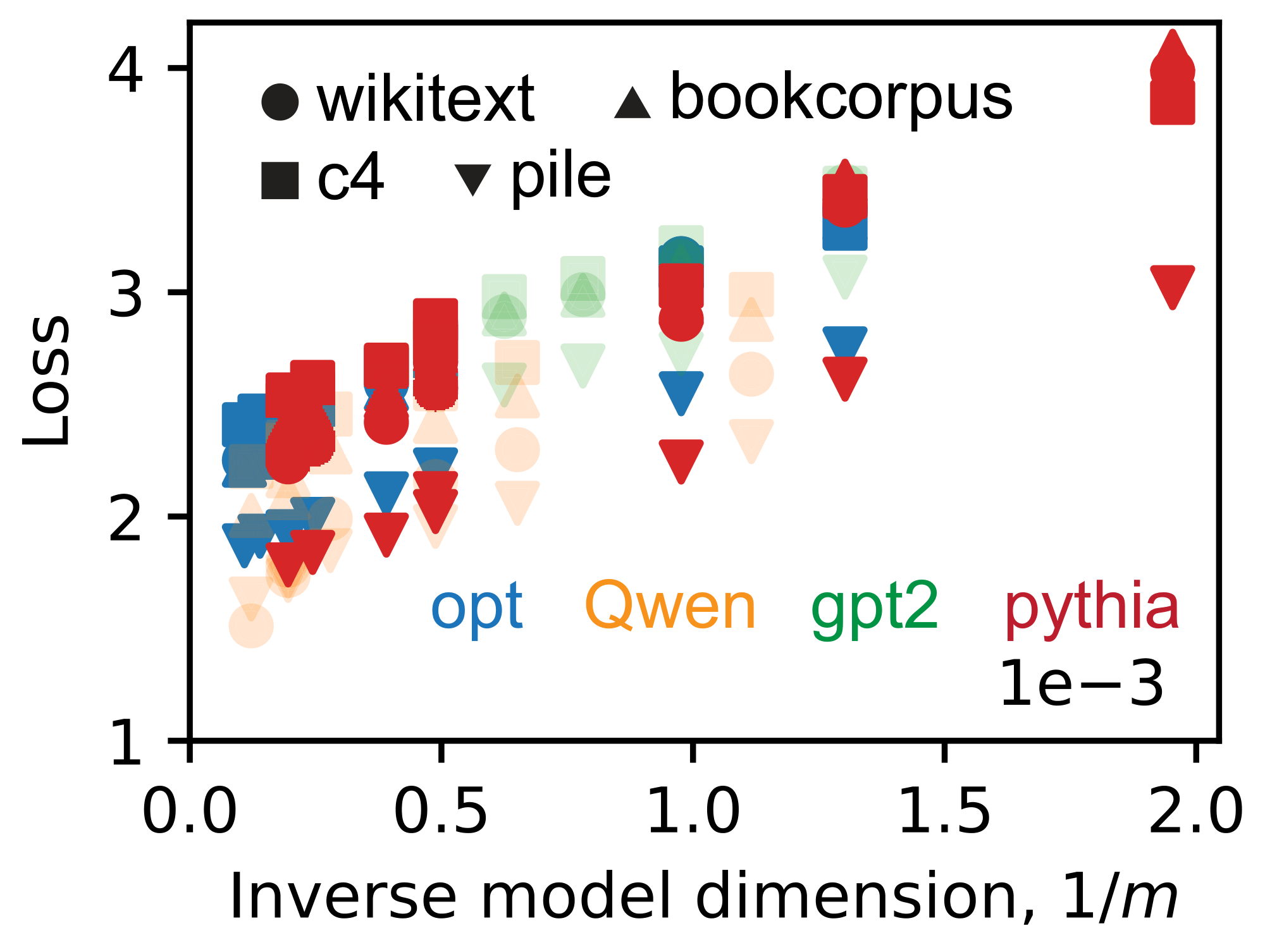
![**Figure 6:** Superposition may explain the neural scaling law observed in actual LLMs. We evaluate four open-sourced model classes, Opt [39], GPT2 [40], Qwen [41], and Pythia [42], which have model sizes from around 100M to 70B (evaluation details in Appendix C). (a) We found the mean square overlaps of $W_i / \|W_i \|_2$ roughly follow $1/m$ scaling, where $W$ is the language model head. (b) The model class is reflected by color as panel a, while we use shapes for evaluation datasets [43, 44, 45, 46]. The loss related to model size is fitted as a power law, yielding empirical $\alpha_m = 0.91\pm 0.04$ close to $1$. More analysis in Appendix D.7.](https://ittowtnkqtyixxjxrhou.supabase.co/storage/v1/object/public/public-images/d3sv9qbk/Fig-6-4.png)
Finally, we explore how our findings might be relevant to real LLMs [39, 40, 41, 42]. As a naive mapping, we treat tokens as atomic features, with data dimension $n$ equal to the vocabulary size. The model dimension $m$ for LLMs is known. We analyze the language model head, denoted by the weight matrix $W$. Through the norm and interference distributions of the rows of $W$, we claim LLMs are in superposition (Appendix D.7). If we measure token frequency, it follows a power law with exponent $\alpha$ close to $1$ (Appendix D.7). We conclude, based on the knowledge from toy models, that LLMs operate in a superposition regime, and expect loss to be related to squared overlaps $\sim 1/m$. We next calculated the mean squared overlaps of normalized rows $W_i/| W_i|_2$, and found they roughly obey $1/m$ scaling (Figure 6 a). We argue that cross-entropy loss, given that the overlaps are small in absolute value, can be expanded and approximately scales as the mean square overlaps (Appendix A.2). We therefore expect the loss of representation-limited LLMs to have $1/m$ scaling. LLM losses are close to a linear function of $1/m$ (Appendix D.7). Yet when $m\to \infty$, the extrapolation of losses does not hit $0$. The non-zero intersection can be due to intrinsic uncertainty in language. Increasing model sizes decreases "wrong" interferences but cannot eliminate uncertainty in the data. So, as in previous papers where loss is decomposed into model size part, dataset size part, and a constant [3], we fit our loss values by the following,
$ L = C_m / m^{\alpha_m} + L_{\backslash m}, $
where the model size part $C_m / m^{\alpha_m}$ is universal (model size is a function of $m$), and $L_{\backslash m}$ contains loss irrelevant to model size, depending on the evaluation dataset and model class. The fitting yields $\alpha_m = 0.91 \pm 0.04$ (Figure 6 b). We inferred from the Chinchilla models [3] that due to model size $N\propto m^{2.52\pm0.03}$ (Appendix D.7), $\alpha_m = (2.52\pm0.03)\times \alpha_N = 0.88 \pm 0.06$, where $\alpha_N = 0.35\pm 0.02$ [47] is the power-law exponent of loss with model size. The exponents $\alpha_m$ from LLMs are close to 1. We highlight the finding as
LLMs operate in the strong superposition regime. The squared overlaps of token representations scale as $1/m$, token frequencies are flat ($\alpha = 1$), and the model size relevant loss scales closely to $1/m$, agreeing with the toy model prediction.
4. Related works
Section Summary: Neural scaling laws describe how the performance of large language models improves in a predictable, power-law manner as models get bigger, datasets grow, or more computing power is used, a pattern observed across many architectures and tasks. Researchers have tried to explain these patterns with simple theoretical models, some focusing on how networks fit the underlying structure of data and others examining limits set by data size or model capacity, often drawing on ideas from statistics and kernel methods. The present work builds on a prior model of how neural networks represent many features in limited space, adapting it to study scaling while differing from earlier studies in compressed sensing and related fields.
Neural scaling laws were first characterized empirically [2], demonstrating that for LLMs, the cross-entropy loss improves predictably as a power-law with increased model size (parameters), dataset size, or compute, over multiple orders of magnitude. This finding is built on earlier observations (e.g. [48]) that deep learning performance scales in a smooth power-law fashion with data and model growth. Many works showed the surprisingly universal nature of such scaling behaviors across architectures and tasks [2, 3, 4], directing further development of LLMs.
Several heuristic toy models have been proposed to explain neural scaling laws. One common view is that models aim to fit data manifolds or functions, and the scaling exponents depend strongly on the structure of the data [14, 15]. Another group of models assumes the network learns discrete features or skills [19, 20], whose importance follows a power-law distribution, giving results the same as ours in the weak superposition regime. One toy model predicts that loss scales inversely with model width [25], arguing that parameters independently perform the same task with noise, and the scaling follows from the central limit theorem. However, this model applies in the overparameterized cases and may be less relevant to LLMs.
More formal approaches rely on similar heuristics. The scaling behavior depends on how the dataset size and model size approach infinity. When the dataset is fixed and model size grows to infinity, the system is variance-limited, and loss scales as $1/m$ by central limit theorem arguments [15]. When the dataset size grows to infinity first, the loss scaling enters the resolution-limited regime. In linear models or kernel methods, this leads to $\alpha_m = \alpha' - 1$ [15, 16, 17, 18], seemingly consistent with our weak superposition regime. Here, $\alpha'$ is the exponent of the power-law decay of kernel eigenvalues, which can be seen as abstract feature importance. Considering neural tangent kernels, $\alpha'$ depends on both data and the model configuration. Our work may be framed as mechanistically showing that $\alpha' = \alpha$ ($\alpha$ is the intrinsic data exponent) when models have no superposition, and $\alpha'$ is something else when models have strong superposition, which is new. The resolution-limited regime has also been described as fitting the data manifold [15].
Our toy model is based on Anthropic’s model of superposition [27] (an autoencoder), with modifications to the data sampling. The original study explored how data structure influences superposition but did not explicitly control it. Related models have appeared in compressed sensing [49, 50, 51, 52, 53] and neural information processing [54, 55], yet with distinct contexts and objectives. Besides representation, people also studied calculation in superposition [56, 57].
5. Discussion
Section Summary: Our analysis is limited because it relies on a simplified toy model without full mathematical solutions, but it indicates that large language models operate in a strong superposition regime driven by sparse language features and the softmax function. We did not examine scaling with data volume or training steps in detail, nor losses from transformer processing layers beyond basic representations; decomposing these shows how geometric interference from superposition can produce the observed power-law scaling with model size. Overall, encouraging superposition may help build more efficient models, though this could hinder interpretability, and the power laws may eventually break once model dimensions approach the vocabulary size.
Our work is built on observations of the toy model and analysis without rigorously solving the toy model. We are thus limited to explaining deeper behaviors in the toy model. Our analysis of LLMs suggests they are in the strong superposition regime, but the underlying reasons were not studied in detail. We believe one reason is that features are sparse in language, as the number of tokens required to predict one token is much less than the total number of tokens. The softmax function may also be important since it is strong at error correction, giving superposition an advantage.
Neural scaling laws also include scaling laws with dataset size and with training steps, which we did not study. At each step, a fixed number of new data points are used for optimization. So, we expect the scaling with the total data amount and that with training steps will be the same, similar to the results at weak superposition [20]. However, in the strong superposition regime, data or training step scaling is related to angle distribution and how angles between representations evolve, which cannot be easily explained without rigorous solving.
We focused on representation loss, yet LLMs should also have losses due to parsing or processing in the transformer layers. We imagine that the loss associated with model size can be written as
$ C_m / m^{\alpha_m} = f_m(m) + f_\ell (\ell), $
where $\ell$ is the depth of the LLM, $f_m$ and $f_\ell$ are two functions capturing the loss due to representation and parsing, respectively. A future direction is to study the parsing-limited scaling (i.e, $f_\ell (\ell)$ function) independently. It is also plausible that the observed scaling of inference time [58] is connected to this parsing-limited regime. We here write the equality because $\ell$ depends on $m$ in LLMs [39, 40, 41, 42]. Given model size $N$, $m$ and $\ell$ are constrained (roughly, $N\propto m^2 \ell$). There is an optimal $m$- $\ell$ relationship such that the loss $f_m(m) + f_\ell (\ell)$ can be minimized given $N$ [59]. At this optimal $m$- $\ell$ relationship, $f_m(m)$ and $f_\ell (\ell)$ should be balanced. Therefore, we expect $f_\ell (\ell)$ to be similar to $f_m(m)$. And if $f_m(m) \sim 1/m$ due to superposition and $f_\ell (\ell)$ is similar, we can measure an empirical $\alpha_m \approx 1$ from data, which is true. Or, if the width-limited loss is much larger, we can also observe that the total loss due to model size has $\alpha_m \approx 1$. We conclude that superposition in any case is an important mechanism underlying neural scaling laws.
Beyond explaining existing phenomena, our results may offer guidance for future LLM development and training strategies:
Assuming our explanation of width scaling is correct, we ask can we change the loss scaling with width to be faster than power laws, or to have larger exponents? The answer is no for natural languages but may be yes for domain tasks with super skewed feature frequencies. Another question is when the scaling law will stop? Based on our naive connection between features and tokens, the answer is that when the model dimension reaches the vocabulary size, the loss limited by width will deviate from a power law and vanish. However, the vocabulary size may set a lower bound for the true number of independent things in language, then the power law with width may continue for a longer time.
Recognizing that superposition benefits LLMs, encouraging superposition could enable smaller models to match the performance of larger ones (with less superposition) and make training more efficient. Architectures such as nGPT [60], which constrain hidden states and weight matrix rows to the unit sphere (promoting superposition), demonstrate improved performance. Optimizers that stabilize training without weight decay have also shown promising results [61], potentially due to enhanced superposition. Yet, these improvements may be related to altering coefficients in the neural scaling laws rather than the exponents. We also acknowledge that encouraging superposition may cause difficulties for the mechanistic interpretation of models and AI safety [27, 62].
As a side note, with the same pre-training loss, LLMs with different degrees of superposition may exhibit differences in emergent abilities such as reasoning or trainability via reinforcement learning [63], requiring future studies.
In conclusion, we studied when loss can be a power law and what the exponent should be with different data properties and degrees of superposition. We found that geometric interference at strong superposition may explain the LLM neural scaling laws observed [3]. Our results contribute to a deeper understanding of modern artificial intelligence systems, which also open various directions for future research. We hope our insights will support the continued development and training of more capable and efficient LLMs.
Acknowledgments
We are grateful for feedback and suggestions from Yasaman Bahri, Cengiz Pehlevan, Surya Ganguli, Blake Bordelon, Daniel Kunin, and the anonymous reviewers. The authors acknowledge the MIT Office of Research Computing and Data for providing high performance computing resources that have contributed to the research results reported within this paper. J. G. thanks the Sloan Foundation for funding. The authors declare no competing interests.
NeurIPS Paper Checklist

Appendix
Section Summary: The appendix analyzes loss scaling in a simplified toy model under strong superposition, considering special data where each point activates exactly one feature. It shows that loss arises mainly from interference between feature vectors and derives how strongly versus weakly represented features produce different scaling behaviors with model size m, including power-law dependence on feature frequency distributions. A similar derivation for cross-entropy loss illustrates that it likewise scales with squared overlaps once vector norms are bounded by data uncertainty.
A. Theoretical analysis
A.1 Toy model loss
We provide a simple analysis for toy model loss scaling. The expected loss in the weak superposition regime is well explained by Equation (4). We do not need to repeat it here.
In the strong superposition regime, we consider an even special data sampling, where data $x$ is sampled such that each data point has and only has one activated feature. The frequency for feature $i$ to be activated is still $p_i$. After determining which feature is activated, say $i$, we still sample $x_i$ as $v_i$ from $U(0, 2)$. This sampling is different from the experiments. Yet, since we learned that activation density does not affect scaling exponent (Figure 14), we expected this analysis to predict at least the scaling exponent. Under the assumptions, we have
$ L = \sum_{i=1}^n p_i \Big\langle \sum_{j\neq i} ReLU^2(W_j\cdot W_i v_i + b_j) + (ReLU(W_i\cdot W_i v_i + b_i) - v_i)^2\Big\rangle_{v_i}.\tag{5} $
We are unable to solve for the optimal $W$ and $b$ such that this loss $L$ is minimized. Yet, it is easy to see that we want $|W_i|_2^2$ to be close to $1$, $W_j\cdot W_i$ to be as small as possible, and $b_j$ to be small negative values of the same order of magnitude as $W_i \cdot W_j$, such that the interference terms $\mathrm{ReLU}(W_j\cdot W_i v_i + b_j)$ may vanish and the recovered feature value $\mathrm{ReLU}(W_i\cdot W_i v_i + b_i)$ can be close to the real one $v_i$.
For convenience, based on the observation that the vector norms are bimodal around $1$ in the strong superposition regime, we define strongly represented features as those that have $|W_i|_2 > 1$, which are more frequent and ETF-like, and weakly represented ones for those with $|W_i|_2 < 1$. We can quantify the fraction of strongly represented as
$ \phi_1 = |{ i : |W_i |_2 > 1 }| / n, $
which significantly exceeds $m/n$ and is around the ETF expectation $m^2 / 2n$ (Figure 16).
We now review our conjectured extreme configuration, consisting of strongly represented and weakly represented features. The first $\phi_1 n$ most important features are considered to be strongly represented, whose absolute overlap with any other representation scales as $\sqrt{1/m}$. The rest of the features are weakly represented and squeezed into a small angle such that they have small overlaps with the strongly represented, while they can have large overlaps with each other. With such a configuration, the first $\phi_1 n$ terms in the summation of Equation (5) will scale as $1/m$ since each term $\langle \cdot s \rangle_{v_i}$ scales as $1/m$. The rest of the terms in Equation (5), in the worst scenario that the terms $\langle \cdot s \rangle_{v_i}$ do not decrease obviously with $m$, will be proportional to $\sum_{i=\phi_i n}^n p_i$. If the strongly represented features dominate, we can have $1/m$ scaling for the loss. On the contrary, when the weakly represented dominate, we expect the loss to have scaling like $\sum_{i=\phi_i n}^n p_i$. More specifically, if $p_i \sim 1 / i^\alpha$ ($\alpha >1$) and we use $m^2/2$ to approximate $\phi_i n$, the loss scales as $1 / m^{2(\alpha -1)}$.
A.2 Cross-entropy loss
We provide the reason why cross-entropy loss also scales as squared overlaps. We consider the last hidden state after going through the normalization layer is $W_i / |W_i |_2$, such that the output should be the $i$ th token. By constructing such an example, we ignore possible loss due to parsing but focus on the loss just due to representation. The loss from this data point is
$ L = -\ln \frac{e^{|W_i |_2}}{\sum_j e^{W_i \cdot W_j / |W_i|2}} = \ln \Big[1 + \sum{j\neq i} e^{W_i \cdot W_j / |W_i|_2 - |W_i |_2} \Big]. $
We assume that $W_i \cdot W_j / |W_i|_2$ is much smaller than $1$ since we know the overlap scale as $1/m$. We then approximate the loss via Taylor expansion
$ L = \ln \Big[1 + (n-1)e^{- |W_i |2} + \sum{j\neq i}[W_i \cdot W_j / |W_i|_2 + (W_i \cdot W_j / |W_i|_2)^2 / 2] e^{- |W_i |_2} \Big]. $
In the first thought, the summation $\sum_{j\neq i}W_i \cdot W_j$ should be zero since there are positive and negative overlaps distributed evenly if the vectors span the whole space. But in language, one sentence can have different continuations, connecting different tokens. For example, both putting "cats" or "dogs" after "I like" are legit. The existence of data "I like" then will tend to squeeze different tokens closer to each other. The summation $W_i \cdot W_j$ should be a small positive constant $\epsilon_{D, i}$ related to the correlation in data. The reason we keep the second-order term is clear now as they are the lowest order terms related to model sizes. We keep expanding the $\ln$ function and have
$ L = (n-1)e^{- |W_i |2} + \frac{\epsilon{D, i}e^{- |W_i |_2}}{|W_i|2}+ \frac{1}{2}\sum{j\neq i}\left(\frac{W_i \cdot W_j}{ |W_i|_2}\right)^2e^{- |W_i |_2}. $
The part related to the model size is mainly
$ L_m = \frac{1}{2}\sum_{j\neq i}\left(\frac{W_i \cdot W_j}{ |W_i|_2}\right)^2e^{- |W_i |_2}. $
In this construction, one can see that once $|W_i |_2$ is sufficiently large, the loss can be arbitrarily low, which does not happen in reality. The reason is still related to the intrinsic uncertainty in language data. If one sentence can have different continuations, we need in the hidden space, a region that can lead to large probabilities over different tokens. However, when the norm is too large, one will find that the hidden space is sharply separated — each hidden state yields high probability only on one token. We then expect the norm $| W_i |_2$ to be as large as possible such that $n e^{-| W_i |_2}$ is small while $| W_i |_2$ is upper bounded by intrinsic data uncertainty. Therefore, $| W_i |_2$ should not depend on model size much (verified in Appendix D.7). The loss related to model size $L_m$ then scales as $1/m$ since the cosine similarity scales as $\sqrt{1/m}$ and $L_m$ is related to the squared cosine similarity in the lowest order approximation.
B. Toy model training
In this Appendix, we explain how we trained the toy models and obtained raw data. There are two classes of toy models trained. The first one is a large toy model with data dimension $n = 10240$, which is reported in Figure 1 and Figure 9 to show scaling behavior across around two orders of magnitude. The other toy model class is small toy models fixing $n = 1000$, such that we can scan more hyperparameters. Figure 3, Figure 4, Figure 5, Figure 14, and Figure 9 use small toy models.
B.1 Large toy models
We implemented a neural network experiment to study the scaling of feature representation and recovery. The toy model is defined as a two-layer neural network with ReLU activation (see Figure 2).
The hyperparameters are give as follows.
- Data dimension $n$: 10240
- Model dimension $m$: Varied exponentially from $2^3$ to $2^{10}$
- Batch size: 2048 (tested up to $8192$, which does not affect final loss)
- Total training steps: 20000 (tested up to $80000$, which does not affect final loss)
- Learning rate: Initially set to 0.02, scaled according to hidden dimension
- Weight decay: $-1.0$ for strong superposition, and $0.1$ for weak superposition
- Device: Training performed using one V100 GPU, with floating-point precision (FP32)
Data points $x$ were synthetically generated at each training step according to Equation (1) to simulate feature occurrence frequencies. We considered three distributions with activation density $E = 1$:
- Exponential: $p_i \propto e^{-i/400}$
- Power-law: $p_i \propto i^{-1.2}$
- Linear: $p_i \propto n - i$
We employed the AdamW optimizer with distinct learning rates and weight decay settings for the weight matrix $W$ and bias vector $b$. Specifically, for weight matrix $W$, learning rate was scaled as $\text{lr} \times (8/m)^{0.25}$ with specified weight decay. And for bias vector $b$, a learning rate of $2.0/m$ was used with no weight decay. A cosine decay learning rate schedule with a warm-up phase (5% of total steps) was implemented. At each training step, input data batches were dynamically generated based on the selected probability distribution. The final test loss is calculated across newly sampled data with a size being $100$ times the batch size.
The model and optimizer were compiled and executed on a CUDA-enabled GPU for efficient training. After training, weight matrices $W$ and training losses were stored and analyzed.
Final outputs, including weight matrices and training loss histories, were saved in PyTorch format for subsequent analysis and visualization.
This setup provided a structured exploration of feature representation scaling under varying dimensions and distributions, crucial for understanding superposition and scaling laws in neural networks.
The code can be found in exp-17.py.
B.2 Small toy models
We conducted numerical simulations using a neural network model designed for feature recovery. The objective was to analyze the model's behavior across various conditions involving feature frequency skewness (controlled by data exponent $\alpha$), model dimensions, and weight decay parameters.
In the small toy models reported in Figure 3, Figure 4, Figure 5, Figure 14, and Figure 9, we set the hyperparameters as
- Feature dimension $ n $ : Fixed at 1000.
- Hidden dimension $ m $ : Varied logarithmically between 10 and 100, across 6 distinct sizes, i.e., $m = 10, 15, 25, 39, 63, 100$.
- Batch size: 2048.
- Training steps: 20000 steps for each condition.
- Learning rate: Initialized at 1 x 10^-2, dynamically adjusted using cosine decay scheduling with a warm-up phase of 2000 steps.
- Weight decay: Explored systematically from -1.0 to 1.0, in increments of 0.22 approximately (10 discrete values).
- Data exponent $\alpha$ : Ranged linearly from 0 to 2, with 17 discrete steps.
In Figure 14, we fix data exponent $\alpha = 1$ while scan $9$ activation densities linearly from $1$ to the maximal value $\sum_{i=1}^n 1/i$. All other settings are the same.
Synthetic data was generated for each batch based on a power-law probability distribution, defined as:
$ p_i \propto \frac{1}{i^{\alpha}} \quad \text{where} \quad i \in {1, 2, \dots, n} $
with the condition $\sum_i p_i = E$ . Each element of the batch data $x$ was randomly activated based on this probability, then scaled by a uniform random value between 0 and 2.
At each training step, input batches were regenerated, and the learning rate was updated following the cosine decay schedule described above.
The training performance was evaluated using Mean Squared Error (MSE) loss computed between the network output and input batch data at every step. Final weights were saved for further analysis. The final test loss is calculated across newly sampled data with a size being $100$ times the batch size.
The simulations were performed in parallel using 96 CPU cores, where each core executed one distinct parameter combination defined by the weight decay and data exponent values. Or, in Figure 14, the parameter combination is defined by weight decay and activation density values.
Loss histories and trained weight matrices were saved separately for post-experiment analysis. Files were systematically indexed to indicate the corresponding experimental parameters. This detailed setup facilitated a comprehensive investigation of model behavior under diverse training and data distribution conditions.
The code can be found in exp-10.py, exp-10-3.py, and exp-15.py.
C. LLM evaluation
C.1 Overlap analysis
We analyzed the row overlaps of the language model head weight matrices among various large language models (LLMs) to investigate the geometric properties of their hidden spaces.
We selected models from the following families, varying widely in parameter count:
- OPT (from OPT-125m to OPT-66b)
- Qwen2.5 (from 0.5B to 72B)
- GPT-2 (GPT2, GPT2-Medium, GPT2-Large, GPT2-XL)
- Pythia (from 70m to 12B)
Weights were downloaded directly from Hugging Face model repositories. For each model, the weight matrix or language modeling head was normalized by its row norms:
$ W_i \leftarrow \frac{W_i}{|W_i|_2 + \epsilon}, \quad \epsilon = 10^{-9}, $
where $\epsilon$ is for numerical stability.
We computed the pairwise absolute cosine overlaps between all normalized vectors using batch-wise computations for efficiency. The overlap between embedding vectors $W_i$ and $W_j$ is given by:
$ \text{overlap}(W_i, W_j) = \left|\frac{W_i \cdot W_j}{|W_i|_2 |W_j|_2}\right|. $
To handle large embedding matrices efficiently, overlaps were computed in batches (size of 8192 vectors).
We calculated two key statistics for the overlaps within each model:
- Mean Overlap: The average of absolute overlaps for all unique vector pairs:
$ \text{mean_overlap} = \frac{\sum_{i<j} \text{overlap}(W_i, W_j)}{n(n-1)/2} $
- Overlap Variance: Calculated as:
$ \text{variance_overlap} = \frac{\sum_{i<j} (\text{overlap}(W_i, W_j) - \text{mean_overlap})^2}{n(n-1)/2} $
From these values, we can calculate mean square overlaps as $\text{mean_overlap}^2 + \text{variance_overlap}$.
The calculations were accelerated using GPU resources (CUDA-enabled) to efficiently handle computations involving extremely large matrices.
Results including mean overlaps, variances, and matrix dimensions were recorded for comparative analysis across model sizes and architectures.
The code is in overlap-0.py.
C.2 Evaluation loss
This experiment aims to evaluate multiple large language models (LLMs) efficiently using model parallelism and dataset streaming techniques. The models were assessed on standard text datasets to measure their predictive performance systematically.
Models were selected from Hugging Face and evaluated using a model-parallel setup:
- OPT series
- Qwen2.5 series
- GPT-2 series
- Pythia series
We used the following publicly available datasets for evaluation:
- Wikitext-103: Standard English language modeling dataset.
- Pile-10k: A subset of The Pile, designed for diverse textual data.
- C4: Colossal Clean Crawled Corpus, containing large-scale web text.
- BookCorpus: Large-scale collection of books used for unsupervised learning.
Datasets were streamed directly, efficiently sampling 10000 text segments with a maximum sequence length of 2048 tokens ($\sim 2 \times 10^7$ tokens).
Texts from datasets were tokenized using the respective model-specific tokenizers. Tokenization involved truncation and manual padding to uniform batch lengths. Specifically, padding tokens were assigned an ID of 0, and label padding utilized a special token (-100) to ensure they did not contribute to loss computations.
Each model was loaded using Hugging Face’s AutoModelForCausalLM with model parallelism enabled, allowing the evaluation of large models that exceed single-GPU memory limits. Evaluations were conducted in batches, employing a DataLoader with a custom collate function for optimized memory use.
The model’s predictive performance was assessed by computing loss values internally shifted by the Hugging Face library, suitable for causal language modeling.
Model parallelism was implemented to efficiently distribute computations across multiple GPUs, leveraging CUDA-enabled hardware.
For each model and each dataset, we run one evaluation and save the evaluation losses.
Random seeds and deterministic sampling ensured reproducible dataset selections, though explicit seed settings were noted as commented options within the implementation.
Evaluation results, including loss metrics and potentially intermediate model states, were systematically stored for detailed post-analysis.
The code is in cali-1.py.
C.3 Token frequency
The purpose of this analysis is to compare token frequencies generated by different tokenizers across several widely-used textual datasets. Understanding these frequencies helps in assessing the representational capacity and efficiency of tokenizers used by various large language models.
We considered the same four datasets mentioned for LLM evaluation. And we use four different tokenizers from the four model classes we evaluated.
Each tokenizer processed textual data from the specified datasets, streaming data directly to efficiently handle large-scale inputs. A target of 1, 000, 000 tokens per tokenizer-dataset pair was set to ensure sufficient statistical representativeness.
For each dataset-tokenizer combination:
- Text samples were streamed directly from the datasets.
- Text was tokenized without adding special tokens (e.g., EOS).
- Token frequencies were counted and accumulated until the target token count (1 million tokens) was reached.
- Token frequencies were saved as JSON files for subsequent detailed analyses.
Token frequency data was systematically stored for each tokenizer and dataset combination, enabling comparative analyses of token distributions. The data files provide foundational insights into tokenizer efficiency and coverage across diverse textual domains.
The code is in token-freq-0.py.
D. Figure details and supplementary results
Here, we show how to process the raw data obtained from toy models or LLMs to generate results seen in the main text. Some supplementary analysis is also conducted to support the main text arguments.
D.1 Figure 1
The toy models reported in Figure 1 are large toy models with data dimension $n = 10240$ explained in Appendix B.1. After obtaining the final losses, we directly plot them with respect to the model dimension $m$. Error bars are calculated as the standard deviation of losses over 100 batches. The error bars are smaller than the dots (Figure 1, b and d).
When we are fitting the loss in log-log as a line, we choose the linear part to fit. If the loss versus model dimension curve is obviously not a line, we fit the whole curve as a line and output the $R^2$ value as a measure of how non-linear it is. Specifically, we fit the last five points for the power-law decay feature case in the weak superposition regime (yellow data in Figure 1 b). Other cases in the weak superposition regime are fitted to a line with all data. In the strong superposition regime, when feature frequency decreases as a power law or as a linear function, we fit the data as a line starting from the third point (yellow and green in Figure 1 d). And for exponential decay feature frequencies, we fit all the data with a line. In the strong superposition regime, the measure model exponent $\alpha_m$ are close to $1$: $1.01\pm 0.05$ (exponential decay), $1.0\pm 0.1$ (power-law decay), and $0.89 \pm 0.05$ (linear decay).
The LLM data are copied from Figure 6 b, with slope $-0.91\pm0.04$ being close to $1$ as well. We will explain details about Figure 6 later.
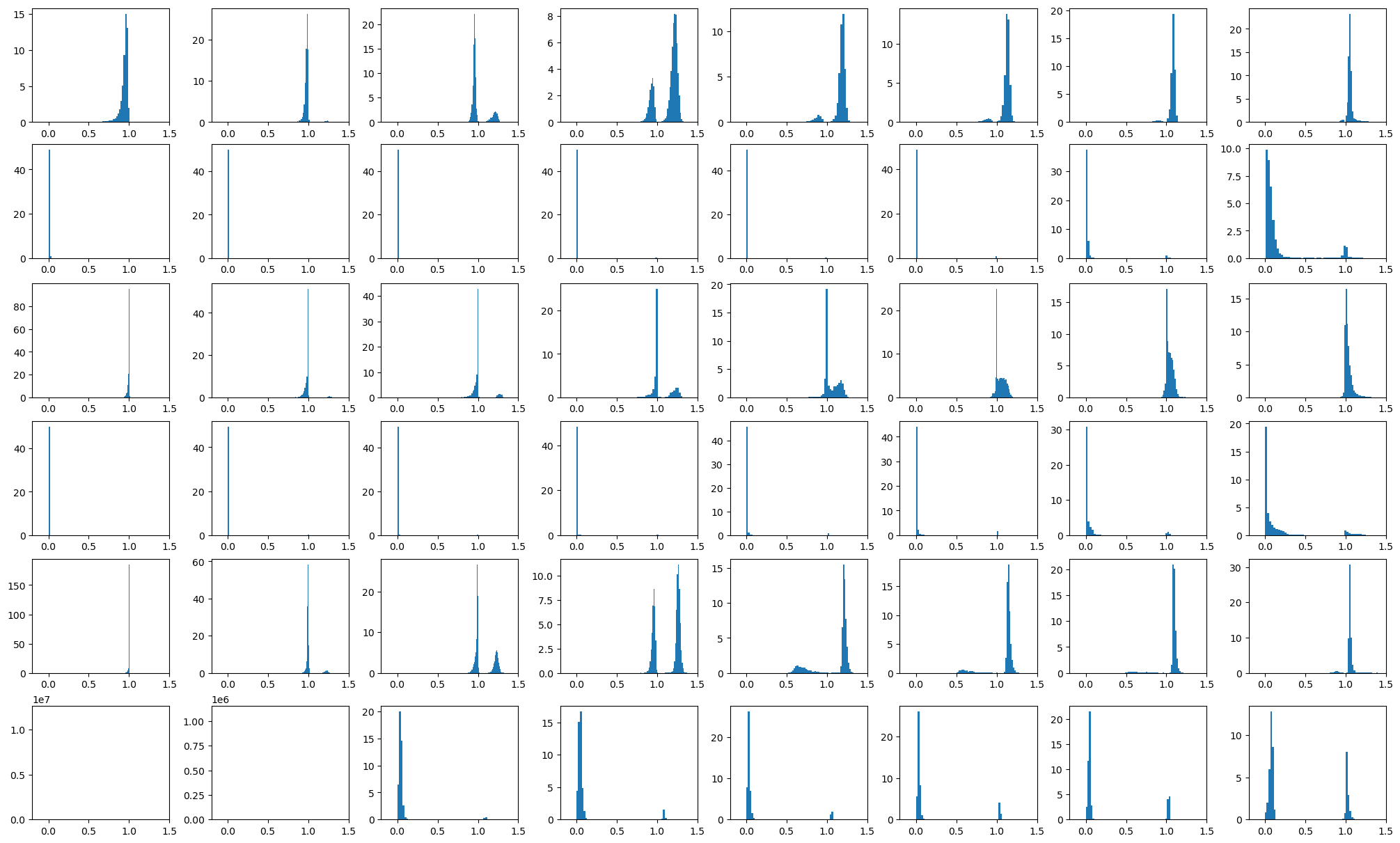
We also output the weight matrix $W$ for these large toy models (Figure 7). They follow the same pattern that in the weak superposition regime, row norms are bimodal and are either close to $0$ or $1$, making $0.5$ a good separation point for measuring how many features are represented. And in the strong superposition regime, the row norms are distributed near $1$, and $1$ is a good separation point for the two peaks, i.e., the peak greater than 1 refers to strongly represented features which are more important, and the peak smaller than 1 corresponds to the weakly represented.
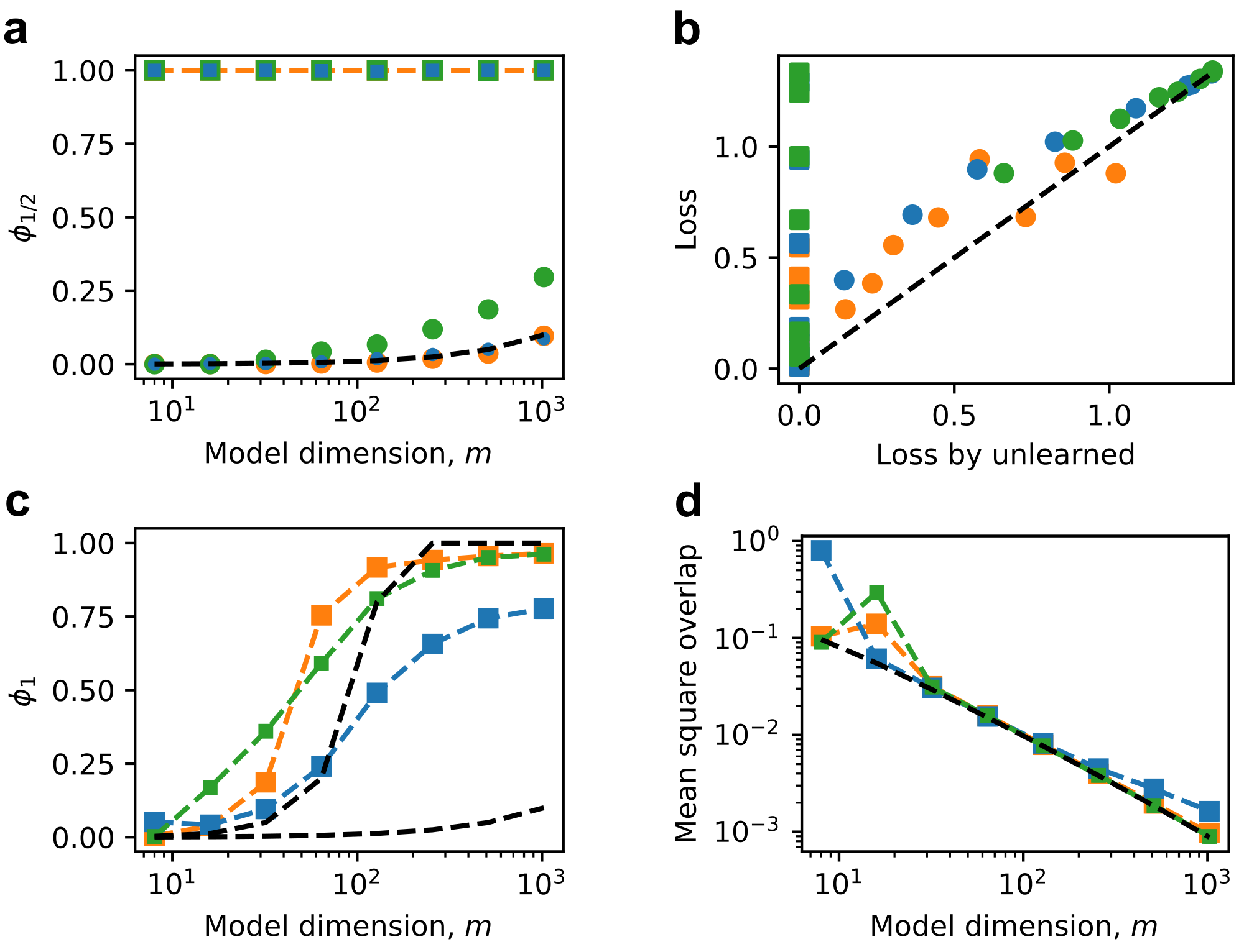
We can analyze the large toy model in the same way as what has been done in Figure 4 and Figure 5. The fraction of represented features $\phi_{1/2}$ is calculated, which is 1 in the strong superposition regime, while it is close to $m/n$ in the weak superposition regime (Figure 8 a).
With the measured $\phi_{1/2}$, we can estimate the loss due to unlearned features, $\langle v^2\rangle\sum_{i = \phi_{1/2}n}^n p_i$. This theoretical value agrees well with the actual loss in the weak superposition regime (Figure 8 b).
In the strong superposition regime, the fraction of strongly represented features is calculated, agreeing with the expectation that the number of strongly represented features is much larger than $m$ but bounded by some value around $m^2/2$ (Figure 8 c).
At the end, we see that the mean square overlap of the strongly represented is close to the characterized value $\kappa^2$ (Figure 8 d), which scales as $1/m$ since the number of the strongly represented is much larger than $m$.
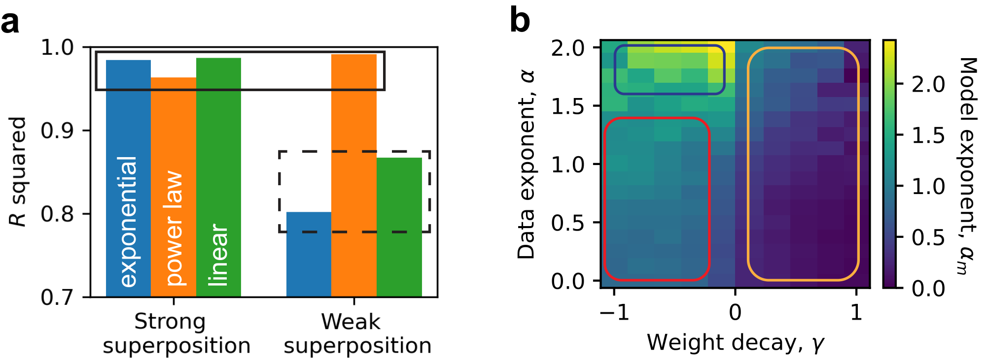
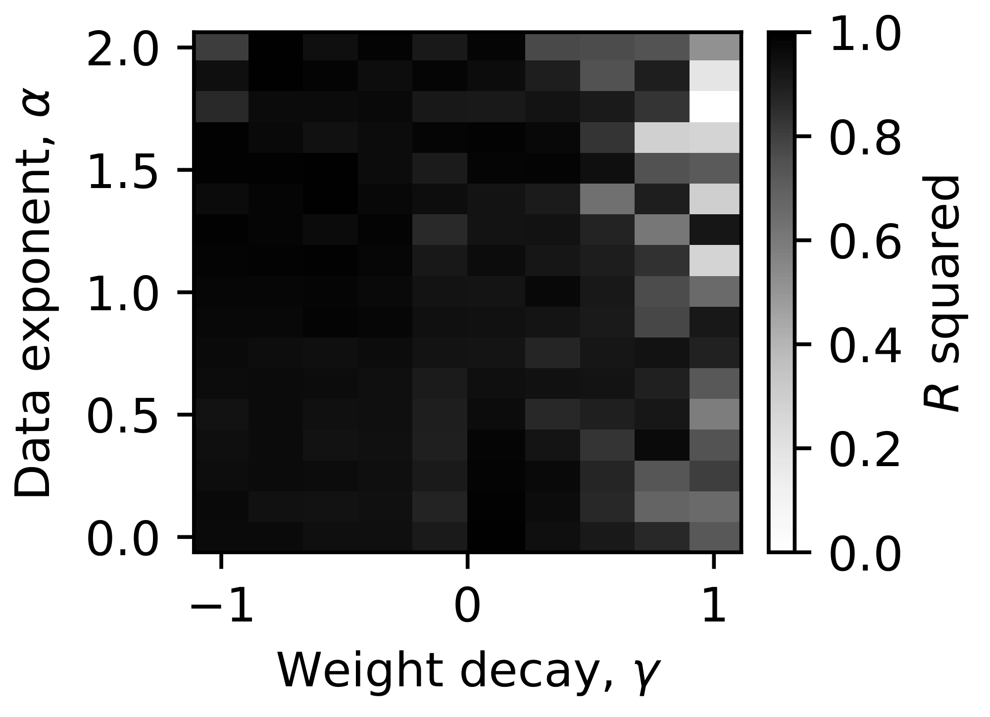
In Figure 1, we set weight decay $\gamma = -1$ to have strong superposition and $\gamma = 0.1$ to have weak superposition. We compute $R$ squared values from linear fits in log-log plots to quantify scaling behavior, assessing how closely the loss follows a power law to model dimension. We can see that at strong superposition, the losses are close to power laws, regardless of the underlying feature frequencies, yet the loss is a power law at weak superposition if the feature frequency $p_i$ is a power law with rank $i$ (Figure 9 a). For a systematic scan, we next set $p_i \propto 1/i^\alpha $ and can vary the data exponent $\alpha$ to change how fast $p_i$ decays consistently. Assuming a power-law form for the final test loss, $L \propto 1 / m^{\alpha_m}$, we extract the model exponent $\alpha_m$ from the empirical fit. We fit the loss with a power law in all cases. The fitted $\alpha_m$ reveals how fast losses decay, even in the regime where the loss should not be a power law. Roughly, three distinct patterns emerge: (1) under weak superposition (positive $\gamma$, yellow box in Figure 9 b), $\alpha_m$ is small, indicating slow loss decay; (2) under strong superposition and a wide range of small data exponents (red box), $\alpha_m$ remains robustly near 1; (3) for strong superposition with large data exponents (blue box), $\alpha_m$ increases with $\alpha$. By interpreting these three patterns, we aim to understand when loss follows a power law with model dimension, and what determines the exponent when it does.
Figure 9 a reports the $R^2$ values from the fitting, where the raw data comes from training large toy models (Appendix B.1). When we are fitting the loss in log-log as a line, we choose the linear part to fit. If the loss versus model dimension curve is obviously not a line, we fit the whole curve as a line and output the $R^2$ value as a measure of how non-linear it is. Specifically, we fit the last five points for the power-law decay feature case in the weak superposition regime (yellow data in Figure 1 b). Other cases in the weak superposition regime are fitted to a line with all data. In the strong superposition regime, when feature frequency decreases as a power law or as a linear function, we fit the data as a line starting from the third point (yellow and green in Figure 1 d).
And from the raw data of small toy models (Appendix B.2), we can fit the model exponent $\alpha_m$ directly and plot it as a function of $\gamma$ and $\alpha$ as in Figure 9 b.
The fitting in Figure 9 b does not care whether the loss versus model dimension curve is a power law or not. We provide the $R$ squared values for the fitting here (Figure 10). The closer $R$ squared values are to $1$, the better the data can be thought to be a power law (a line in log-log plot). In the strong superposition regime, the $R$ squared values suggest the data are close to be power-law. While in the weak superposition regime, data may not be power-law, especially when $\gamma$ is too large. When $\alpha$ is smaller than $1$, it is not a power law in theory. The $R$ squared values are not too small since the loss decay is very slow, and a line in log-log plot is still a good approximation. When $\alpha >1$ and $\gamma \approx 1$, the number of represented features can be smaller than $m$ or even non-increasing. Too large weight decay still makes the configuration of the representation be in no superposition. However, it destroys some feature representations that can exist, making the configuration far from the ideal case where $m$ features are represented. So, we may not see power laws when weight decay is too strong.
D.2 Figure 2
Figure 2 introduced the toy model and the concept of superposition without real data. The $W$ matrix we used to show superposition in Figure 2 c is obtained by optimizing the square of off-diagonal terms of the normalized $W$, i.e., each row is normalized to have norm 1 first.
D.3 Figure 3
In Figure 3, we reported results from the trained small toy models with data dimension $n = 1000$, whose detailed hyperparameters are in Appendix B.2.
We showed results at data exponent $\alpha = 1$ in Figure 3. The results are obtained at $m =100$, $\gamma = -1$ for panel a, and at different $m$ and $\gamma$ for panel b. We showed that the more frequent features tend to have larger norms or to be better represented. And the norm distribution is very bimodal. We here show that it is true that the norm is around $1$ or $0$ for various $\alpha$ and model sizes $m$ and degrees of superposition (Figure 11 and Figure 12). The fraction of represented, $\phi_{1/2}$, can be calculated directly.
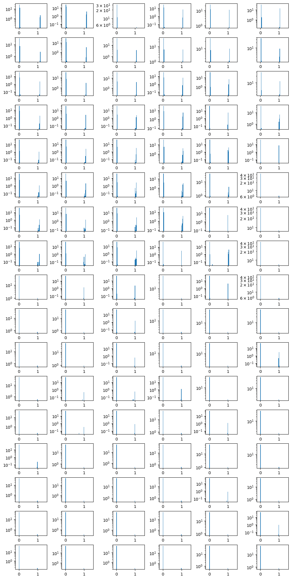
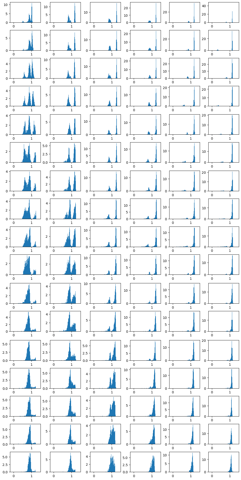
Here, we provide the heat map of $\phi_{1/2}$ at different $m$ as a function of $\alpha$ and $\gamma$ (Figure 13). The pattern is robust, suggesting weight decay is a good tool to change the degree of superposition regardless of data properties and model sizes.

D.4 Sparsity does not affect scaling behaviors in our tests
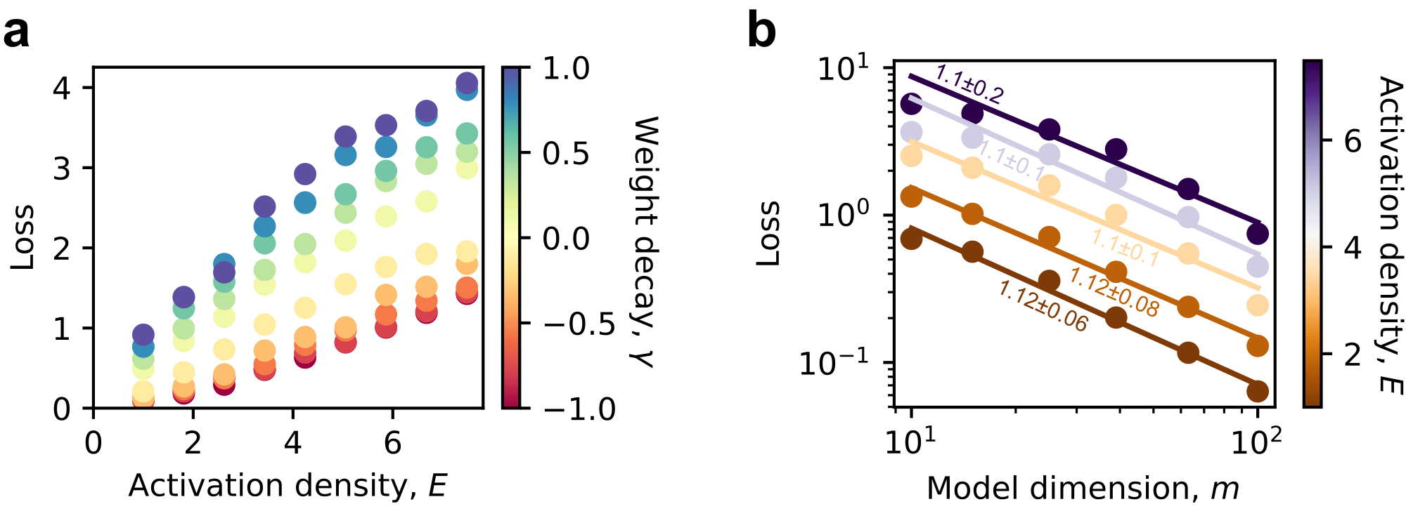
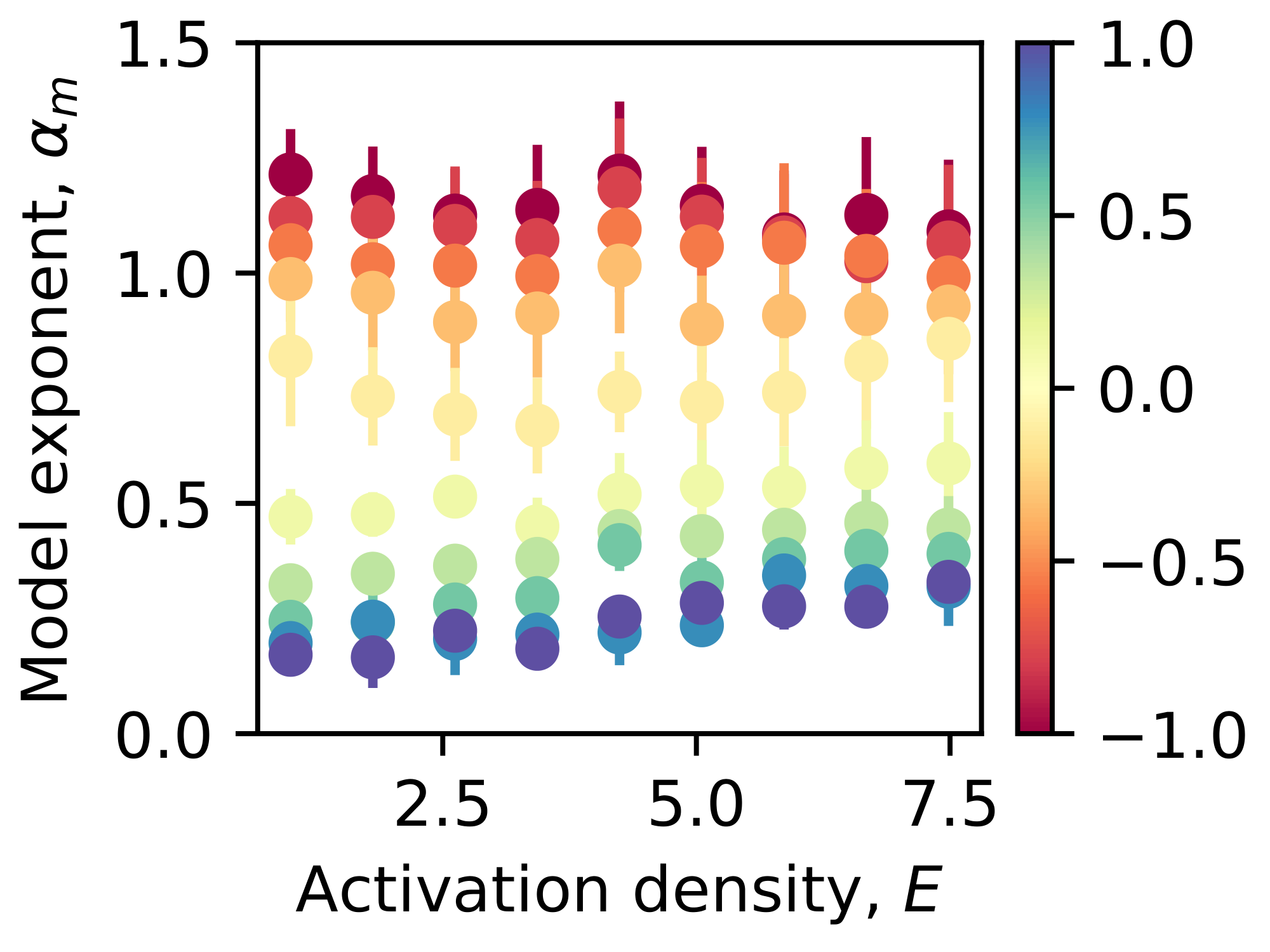
We studied the effect of the number of expected activated features or activation density $E$, which was set to $1$. By fixing data exponent $\alpha = 1$, which will be shown to be relevant to natural language, we can scan different superposition degrees and activation densities. Since $p_i \leq 1$ is required, which is equivalent to $p_1\leq 1$, we have $E \leq \sum_{i=1}^n 1/i^\alpha$, setting the upper bound for our scanning. We found that loss is approximately proportional to activation density $E$ (Figure 14 a). This fact suggests that the power law exponent should not change, which we confirmed (Figure 14 b). Under a controlled superposition degree, activation density linearly increases loss and thus does not affect the scaling exponents in our experiments.
Once obtaining the small toy models scanning activation density and keeping $\alpha = 1$, we can plot the loss as a function of activation density $E$ in Figure 14. The linear fitting is also straightforward. We chose one $\gamma$ to show in the main text. Here, we present the whole picture that, with any weight decay tested, the model exponent is robust to the change of activation density (Figure 15).
D.5 Figure 4
In Figure 4 a, we plot the raw losses from small toy model experiments (hyperparameters in Appendix B.2). The theoretical value of loss is approximated by an integral $\int_{n\phi_{1/2}}^n 1/i^{\alpha} \mathrm{d}i$, which is
$ L = \left{ \begin{aligned} &\frac{\phi_{1/2}^{1-\alpha} - 1}{1 - n^{1-\alpha}}n^{1-\alpha}, ~ \alpha \neq 1, \ &-\frac{\ln \phi_{1/2}}{\ln n}, ~ \alpha = 1. \end{aligned} \right. $
To quantify how much the learned weight matrix deviates from the ideal no superposition structure, we construct a reference matrix and compute a norm difference. Specifically, we first create an $n$-by- $n$ zero matrix called base, and then insert an identity matrix of size $m$ in its top-left corner. This padded identity matrix serves as a reference for the perfect recovery of the first $m$ features. We then compute the matrix product $WW^T$ from the learned weights and compare it to this reference using the matrix 2-norm. The resulting value reflects the ambiguity or interference in the learned representations. We store this norm in the ambiguity tensor at the location indexed by the current task and model width. Given a weight decay and data exponent, we have 6 ambiguity values since we have 6 $m$ values. We calculate maximum ambiguity among these 6 models, and choose the 9 cases with the smallest maximum ambiguity to plot in Figure 4 b. One can see that when weight decay is near $0.5$, the models are closest to the ideal no superposition case where the first $m$ features are represented perfectly. Smaller weight decay may not be sufficient to eliminate superposition, and larger weight decay can suppress features that, in principle, can be represented perfectly.
D.6 Figure 5
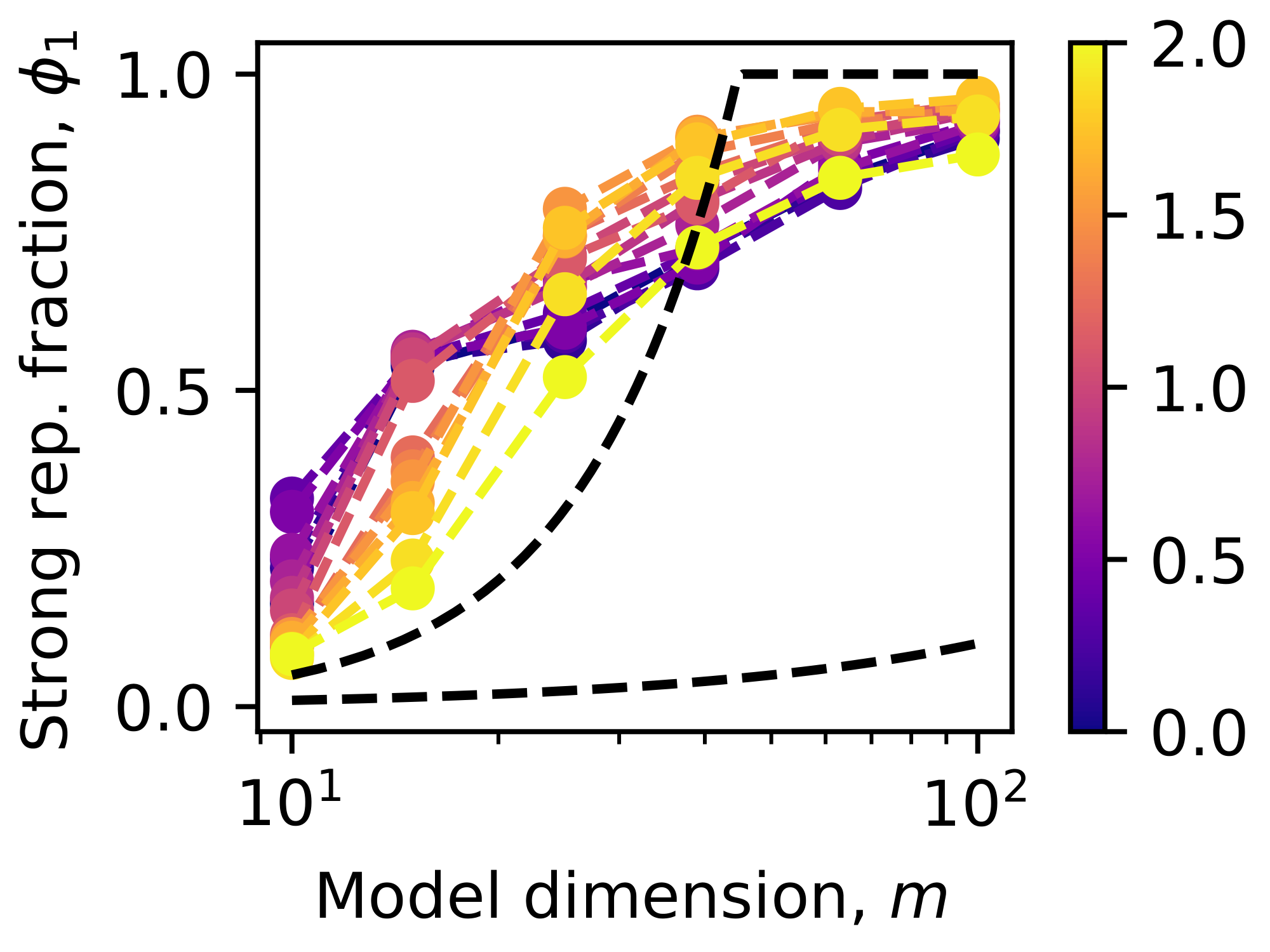
For convenience, based on the observation that the vector norms are bimodal around $1$ in the strong superposition regime, we define strongly represented features as those that have $|W_i|_2 > 1$, which are more frequent and ETF-like, and weakly represented ones for those with $|W_i|_2 < 1$. We can quantify the fraction of strongly represented as
$ \phi_1 = |{ i : |W_i |_2 > 1 }| / n, $
which significantly exceeds $m/n$ and is around the ETF upper bound $m^2 / 2n$ (Figure 16). The group of vectors $| W_i|_2$ with norm greater than 1 or the strongly represented features then roughly agree with ETF properties: small variance, $1/m$ mean squared overlaps, and a limited number of vectors.
Figure 5 studies the results from small toy models (Appendix B.2) focusing on the strong superposition regime. For the strongly represented fraction, $\phi_1$, we can directly compute based on the definition and the obtained weight matrices. We showed a row norm distribution at $m = 15$, $\alpha = 1$, and $\gamma = -0.78$ in Figure 5 panels a and b. Here, we provide more data to show that 1 is a natural separation point in norm to determine which are strongly represented and which are weakly represented (Figure 12).
Once select the rows with norm greater than 1, we can calculate their mean and variance of squared overlaps based on normalized rows $W_i / | W_i|_2$ (Figure 5, c and d). We argue that after training, the vectors will be more similar to ETFs than to random initialization. This is studied via the variance of overlaps. ETFs, in theory, have zero variance. We find that the majority of the overlap variances are much smaller than the random initialization, especially when features have similar frequencies, which agrees with the expectation. The cases where the actual variance is greater than that of the random vectors have large $\alpha$, roughly correspond to the cases where $\alpha_m$ deviates from $1$ — ETF-like configuration no longer dominates. This is intuitive that when $\alpha$ is too large, the heterogeneity of overlaps will become large — it is better to let more frequent features occupy larger angle space. We argue that the large variance at large $\alpha$ does not mean the configuration tends to be random, but tends to be something more closely related to the frequency distribution of the features.
Our explanations based on the strongly and weakly represented features capture the basic trend that when $\alpha$ is getting large, the more important features will have larger angle space and the loss decay will be more related to the data exponent. However, this theory is oversimplified, where the strongly represented all have small overlaps and the weakly represented all have large overlaps. The real situation may be more like the angle occupied by one feature decreases continuously as the frequency decreases. As suggested by Figure 5 c, overlap variance within the strongly represented is greater when $\alpha$ is larger. To be more precise about the overlap distribution as well as the exponent $\alpha_m$ when $\alpha$ is large, we cannot use simple theoretical expectations like ETFs but have to solve the toy model.
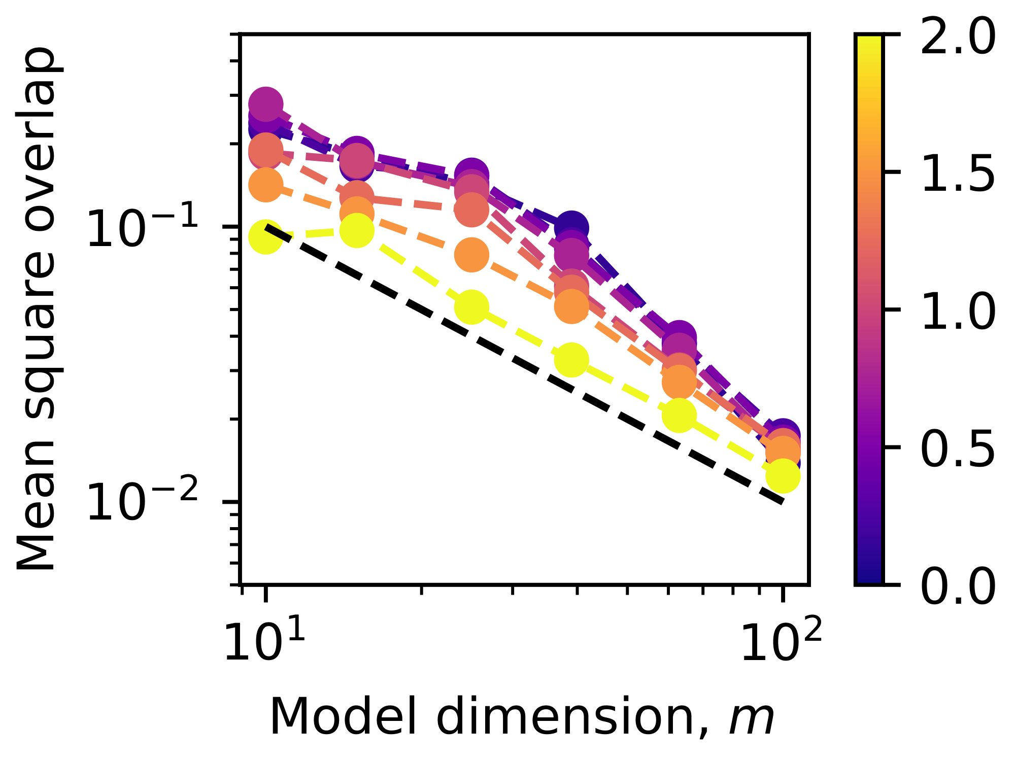
We also provide evidence that overlaps of all the vectors (Figure 17). We see that some of the mean square overlaps are larger than $1/m$ instead of being on the line $1/m$. However, all the mean values follow $1/m$ scaling even for large $\alpha$ cases where the vectors are no longer isotropic. We emphasize that for even frequencies and isotropic vectors, since squared overlaps scale as $1/m$, the loss should scale as $1/m$.
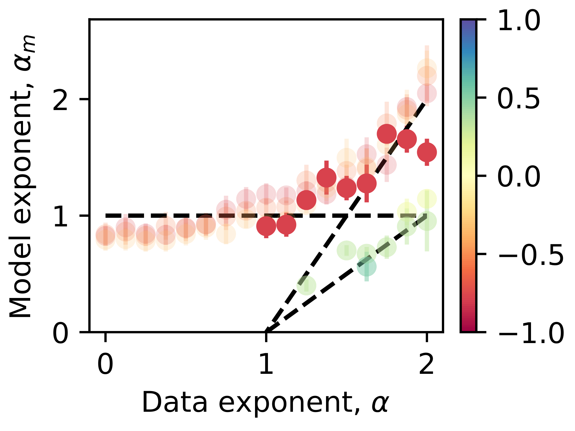
After fitting $\alpha_m$ of the trained small toy models (Appendix B.2), we plotted the $\alpha_m$ corresponding to the second to the fourth smallest weight decays in Figure 5 e. We also copied from Figure 4 b and plotted the ideal weak superposition case in Figure 5 e. One question we had is that if $m^2/2$ is always greater than $n$, in our analysis, all vectors can be strongly represented, what should $\alpha_m$ be? We trained the small toy models again as in Appendix B.2 but with $m$ from $50$ to $150$. We found that in the strong superposition regime, the $\alpha_m$ is still around $1$ when $\alpha$ is smaller than $1.5$, and $\alpha_m$ still increases a little while smaller than $2(\alpha -1)$ when $\alpha$ is larger than $1.5$ (Figure 18). When $m^2/2n >1$ is always true, the vectors can be put into a configuration where all overlaps are small and scale as $\sqrt{1/m}$, such that $\alpha_m$ should be closer to $1$. However, as mentioned before, our picture that the strongly represented have nearly uniform absolute overlaps is oversimplified. In the real situation, more frequent features have smaller or even faster decaying overlaps. Therefore, when $\alpha$ is too large, a weighted sum of squared overlaps, weighting the more frequent features more, can decrease faster than the average decaying speed $1/m$. Again, we need to solve the toy model faithfully to uncover the rigorous relation between $\alpha_m$ and $\alpha$ and argue the robustness of $\alpha_m$ from theory.
D.7 Figure 6
After obtaining the overlaps as described in Appendix C.1, we directly plot the raw data in Figure 6 a. The data are quite noisy, and we did not fit the data with a line.
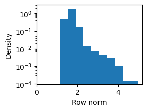
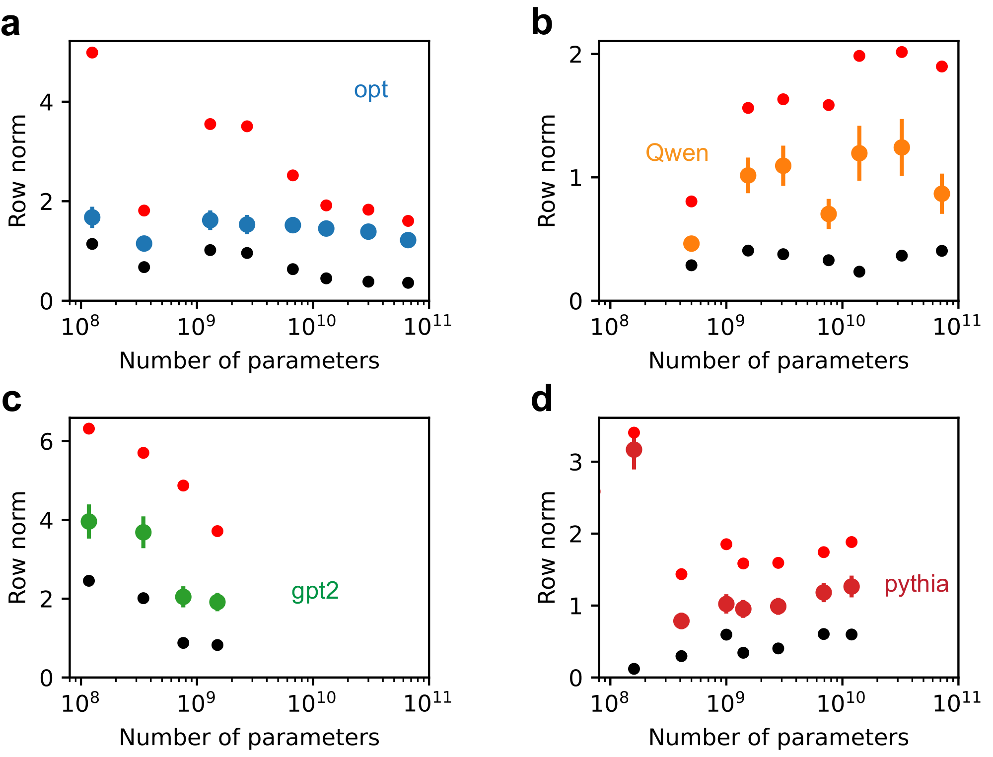
We argued that the LLMs are in the strong superposition regime since all tokens are represented. Figure 19 shows a typical row norm distribution of LLM (opt, 125M parameters [39]). We showed the mean, minimum, and maximum row norms of all the LLMs studied in Figure 20. From the non-zero minimum norms and the fact $n \gg m$, we confirm LLMs are in strong superposition. As mentioned in the analysis in Appendix A.2, we argue that the row norm of LLMs should not depend on $m$ but controlled more by the intrinsic data property of language, which is also verified to be valid (Figure 20).
We obtain the evaluation loss of each model on each dataset as described in Appendix C.2. We fit our loss values by the formula,
$ L = C_m / m^{\alpha_m} + L_{\backslash m}, $
where $C_m / m^{\alpha_m}$ is universal and $L_{\backslash m}$ is a constant depending on the dataset and model class. There are in total $16$ different $L_{\backslash m}$ since we have $4$ different model classes and 4 datasets. In our fitting model, there are in total $18$ parameters. We use Adam to minimize the mean square error between the predicted loss by the above function and the real loss. All losses obtained are used in optimization. The code is in nonlinearfit-3.ipynb.
We provide the raw data, losses, as a function of $1/m$ (Figure 21). The losses looks like a line with $1/m$ in one model class and with the same dataset. And the slope of the line seems to be universal. These two points support us in proposing the formula above, where $C_m / m^{\alpha_m}$ is universal. The intersections are different depending on the dataset and model class, corresponding to different $L_{\backslash m}$.
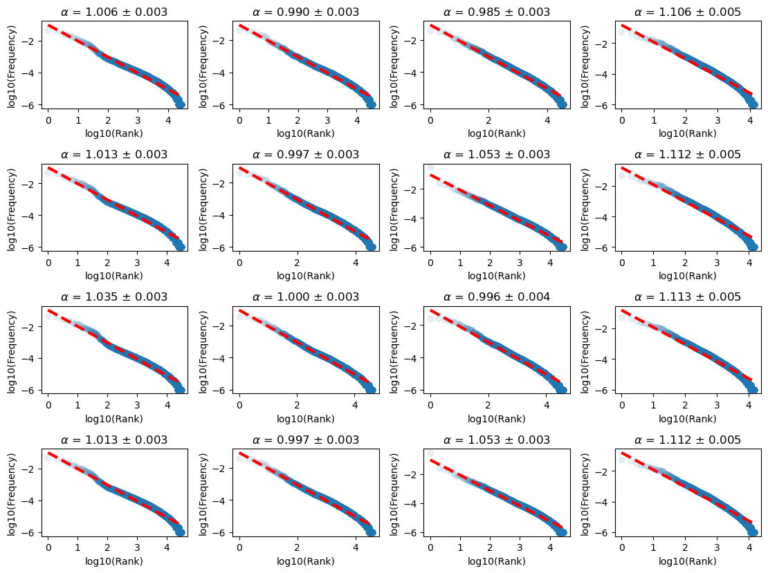
We obtained the token frequencies as described in Appendix C.3. Given the raw data, we sort the token frequency and obtain the frequency-rank plot. We sample 1000 (this number does not matter once it is large, 10000 gives the same result) points uniformly in the $\log_{10}$ (Rank), and fit the frequency-rank as a power law, or a line in log-log plot. Results show that the data exponent fitted $\alpha$ is close to $1$ regardless of the dataset or the tokenizer (Figure 22).
We study the relationship between model dimension $m$ and model size $N$ (number of parameters). For the four open-sourced models we analyzed [39, 40, 41, 42], we can see that $N\sim m^3$, especially when $m$ is large. If we fit the $N$- $m$ relation by a power law while assuming a universal exponent but different coefficients depending on the model class, we obtain an exponent of $2.51$ (Figure 23 a). For the Chinchilla model reported in [3], we find $N$ is also close to a power law with the model dimension, and the fitted exponent is $2.52\pm 0.03$ (Figure 23 b).
![**Figure 23:** The model size is approximately a power law with model dimension. (a) The four model classes we analyzed [39, 40, 41, 42]. (b) The Chinchilla models [3].](https://ittowtnkqtyixxjxrhou.supabase.co/storage/v1/object/public/public-images/d3sv9qbk/Fig-8-s-5.png)
References
Section Summary: This section compiles a numbered list of academic papers, preprints, and technical reports focused on large language models and neural networks. The works examine topics such as model scaling with increased data and compute, few-shot learning capabilities, and applications in areas like science, mathematics, and code generation. Many entries also explore the underlying mathematical and empirical explanations for why these systems improve predictably as they grow larger.
[1] Tom Brown, Benjamin Mann, Nick Ryder, Melanie Subbiah, Jared D Kaplan, Prafulla Dhariwal, Arvind Neelakantan, Pranav Shyam, Girish Sastry, Amanda Askell, et al. Language models are few-shot learners. Advances in neural information processing systems, 33:1877–1901, 2020.
[2] Jared Kaplan, Sam McCandlish, Tom Henighan, Tom B Brown, Benjamin Chess, Rewon Child, Scott Gray, Alec Radford, Jeffrey Wu, and Dario Amodei. Scaling laws for neural language models. arXiv preprint arXiv:2001.08361, 2020.
[3] Jordan Hoffmann, Sebastian Borgeaud, Arthur Mensch, Elena Buchatskaya, Trevor Cai, Eliza Rutherford, Diego de Las Casas, Lisa Anne Hendricks, Johannes Welbl, Aidan Clark, et al. Training compute-optimal large language models. arXiv preprint arXiv:2203.15556, 2022.
[4] Tom Henighan, Jared Kaplan, Mor Katz, Mark Chen, Christopher Hesse, Jacob Jackson, Heewoo Jun, Tom B Brown, Prafulla Dhariwal, Scott Gray, et al. Scaling laws for autoregressive generative modeling. arXiv preprint arXiv:2010.14701, 2020.
[5] Josh Achiam, Steven Adler, Sandhini Agarwal, Lama Ahmad, Ilge Akkaya, Florencia Leoni Aleman, Diogo Almeida, Janko Altenschmidt, Sam Altman, Shyamal Anadkat, et al. Gpt-4 technical report. arXiv preprint arXiv:2303.08774, 2023.
[6] Haotong Qin, Ge-Peng Ji, Salman Khan, Deng-Ping Fan, Fahad Shahbaz Khan, and Luc Van Gool. How good is google bard's visual understanding? an empirical study on open challenges. arXiv preprint arXiv:2307.15016, 2023. https://arxiv.org/abs/2307.15016.
[7] Aitor Lewkowycz, Anders Andreassen, David Dohan, Ethan Dyer, Henryk Michalewski, Vinay Ramasesh, Ambrose Slone, Cem Anil, Imanol Schlag, Theo Gutman-Solo, et al. Solving quantitative reasoning problems with language models. Advances in neural information processing systems, 35:3843–3857, 2022.
[8] Ross Taylor, Marcin Kardas, Guillem Cucurull, Thomas Scialom, Anthony Hartshorn, Elvis Saravia, Andrew Poulton, Viktor Kerkez, and Robert Stojnic. Galactica: A large language model for science. arXiv preprint arXiv:2211.09085, 2022.
[9] Stephen Wolfram. Wolfram|alpha as the computation engine for gpt models, 2023. https://www.wolfram.com/wolfram-alpha-openai-plugin.
[10] Trieu H Trinh, Yuhuai Wu, Quoc V Le, He He, and Thang Luong. Solving olympiad geometry without human demonstrations. Nature, 625(7995):476–482, 2024.
[11] Mark Chen, Jerry Tworek, Heewoo Jun, Qiming Yuan, Henrique Ponde De Oliveira Pinto, Jared Kaplan, Harri Edwards, Yuri Burda, Nicholas Joseph, Greg Brockman, et al. Evaluating large language models trained on code. arXiv preprint arXiv:2107.03374, 2021.
[12] GitHub. Github copilot: Your ai pair programmer, 2022. https://github.com/features/copilot.
[13] Jack W Rae, Sebastian Borgeaud, Trevor Cai, Katie Millican, Jordan Hoffmann, Francis Song, John Aslanides, Sarah Henderson, Roman Ring, Susannah Young, et al. Scaling language models: Methods, analysis & insights from training gopher. arXiv preprint arXiv:2112.11446, 2021.
[14] Utkarsh Sharma and Jared Kaplan. Scaling laws from the data manifold dimension. Journal of Machine Learning Research, 23(9):1–34, 2022.
[15] Yasaman Bahri, Ethan Dyer, Jared Kaplan, Jaehoon Lee, and Utkarsh Sharma. Explaining neural scaling laws. Proceedings of the National Academy of Sciences, 121(27):e2311878121, 2024.
[16] Blake Bordelon, Abdulkadir Canatar, and Cengiz Pehlevan. Spectrum dependent learning curves in kernel regression and wide neural networks. In International Conference on Machine Learning, pages 1024–1034. PMLR, 2020.
[17] Blake Bordelon, Alexander Atanasov, and Cengiz Pehlevan. How feature learning can improve neural scaling laws. Journal of Statistical Mechanics: Theory and Experiment, 2025(8):084002, 2025.
[18] Alexander Maloney, Daniel A Roberts, and James Sully. A solvable model of neural scaling laws. arXiv preprint arXiv:2210.16859, 2022.
[19] Marcus Hutter. Learning curve theory. arXiv preprint arXiv:2102.04074, 2021.
[20] Eric Michaud, Ziming Liu, Uzay Girit, and Max Tegmark. The quantization model of neural scaling. Advances in Neural Information Processing Systems, 36:28699–28722, 2023.
[21] Ziming Liu, Yizhou Liu, Eric J Michaud, Jeff Gore, and Max Tegmark. Physics of skill learning. arXiv preprint arXiv:2501.12391, 2025.
[22] Danny Hernandez, Tom Brown, Tom Conerly, Nova DasSarma, Dawn Drain, Sheer El-Showk, Nelson Elhage, Zac Hatfield-Dodds, Tom Henighan, Tristan Hume, et al. Scaling laws and interpretability of learning from repeated data. arXiv preprint arXiv:2205.10487, 2022.
[23] Ari Brill. Neural scaling laws rooted in the data distribution. arXiv preprint arXiv:2412.07942, 2024.
[24] Stefano Spigler, Mario Geiger, and Matthieu Wyart. Asymptotic learning curves of kernel methods: empirical data versus teacher–student paradigm. Journal of Statistical Mechanics: Theory and Experiment, 2020(12):124001, 2020.
[25] Jinyeop Song, Ziming Liu, Max Tegmark, and Jeff Gore. A resource model for neural scaling law. arXiv preprint arXiv:2402.05164, 2024.
[26] Sanjeev Arora, Yuanzhi Li, Yingyu Liang, Tengyu Ma, and Andrej Risteski. Linear algebraic structure of word senses, with applications to polysemy. Transactions of the Association for Computational Linguistics, 6:483–495, 2018.
[27] Nelson Elhage, Tristan Hume, Catherine Olsson, Nicholas Schiefer, Tom Henighan, Shauna Kravec, Zac Hatfield-Dodds, Robert Lasenby, Dawn Drain, Carol Chen, Roger Grosse, Sam McCandlish, Jared Kaplan, Dario Amodei, Martin Wattenberg, and Christopher Olah. Toy models of superposition. Transformer Circuits Thread, 2022.
[28] Ilya Loshchilov and Frank Hutter. Decoupled weight decay regularization. arXiv preprint arXiv:1711.05101, 2017.
[29] Lloyd Welch. Lower bounds on the maximum cross correlation of signals (corresp.). IEEE Transactions on Information Theory, 20(3):397–399, 2003.
[30] Peter G Casazza and Gitta Kutyniok. Finite frames: Theory and applications. Springer Science & Business Media, 2012.
[31] Thomas Strohmer and Robert W Heath Jr. Grassmannian frames with applications to coding and communication. Applied and computational harmonic analysis, 14(3):257–275, 2003.
[32] Matthew Fickus, Dustin G Mixon, and Janet C Tremain. Steiner equiangular tight frames. Linear algebra and its applications, 436(5):1014–1027, 2012.
[33] Joseph M Renes, Robin Blume-Kohout, A J Scott, and Carlton M Caves. Symmetric informationally complete quantum measurements. Journal of Mathematical Physics, 45(6):2171–2180, 2004.
[34] Yizhou Liu and John B. DeBrota. Relating measurement disturbance, information, and orthogonality. Phys. Rev. A, 104:052216, Nov 2021.
[35] Yizhou Liu and Shunlong Luo. Quantifying unsharpness of measurements via uncertainty. Phys. Rev. A, 104:052227, Nov 2021.
[36] Yizhou Liu, Shunlong Luo, and Yuan Sun. Total, classical and quantum uncertainties generated by channels. Theoretical and Mathematical Physics, 213(2):1613–1631, 2022.
[37] Vardan Papyan, XY Han, and David L Donoho. Prevalence of neural collapse during the terminal phase of deep learning training. Proceedings of the National Academy of Sciences, 117(40):24652–24663, 2020.
[38] Vignesh Kothapalli. Neural collapse: A review on modelling principles and generalization. arXiv preprint arXiv:2206.04041, 2022.
[39] Susan Zhang, Stephen Roller, Naman Goyal, Mikel Artetxe, Moya Chen, Shuohui Chen, Christopher Dewan, Mona Diab, Xian Li, Xi Victoria Lin, et al. Opt: Open pre-trained transformer language models. arXiv preprint arXiv:2205.01068, 2022.
[40] Alec Radford, Jeffrey Wu, Rewon Child, David Luan, Dario Amodei, Ilya Sutskever, et al. Language models are unsupervised multitask learners. OpenAI blog, 1(8):9, 2019.
[41] An Yang, Baosong Yang, Beichen Zhang, Binyuan Hui, Bo Zheng, Bowen Yu, Chengyuan Li, Dayiheng Liu, Fei Huang, Haoran Wei, Huan Lin, Jian Yang, Jianhong Tu, Jianwei Zhang, Jianxin Yang, Jiaxi Yang, Jingren Zhou, Junyang Lin, Kai Dang, Keming Lu, Keqin Bao, Kexin Yang, Le Yu, Mei Li, Mingfeng Xue, Pei Zhang, Qin Zhu, Rui Men, Runji Lin, Tianhao Li, Tingyu Xia, Xingzhang Ren, Xuancheng Ren, Yang Fan, Yang Su, Yichang Zhang, Yu Wan, Yuqiong Liu, Zeyu Cui, Zhenru Zhang, and Zihan Qiu. Qwen2.5 technical report. arXiv preprint arXiv:2412.15115, 2024.
[42] Stella Biderman, Hailey Schoelkopf, Quentin Gregory Anthony, Herbie Bradley, Kyle O’Brien, Eric Hallahan, Mohammad Aflah Khan, Shivanshu Purohit, USVSN Sai Prashanth, Edward Raff, et al. Pythia: A suite for analyzing large language models across training and scaling. In International Conference on Machine Learning, pages 2397–2430. PMLR, 2023.
[43] Stephen Merity, Caiming Xiong, James Bradbury, and Richard Socher. Pointer sentinel mixture models. arXiv preprint arXiv:1609.07843, 2016.
[44] Leo Gao, Stella Biderman, Sid Black, Laurence Golding, Travis Hoppe, Charles Foster, Jason Phang, Horace He, Anish Thite, Noa Nabeshima, et al. The pile: An 800gb dataset of diverse text for language modeling. arXiv preprint arXiv:2101.00027, 2020.
[45] Colin Raffel, Noam Shazeer, Adam Roberts, Katherine Lee, Sharan Narang, Michael Matena, Yanqi Zhou, Wei Li, and Peter J Liu. Exploring the limits of transfer learning with a unified text-to-text transformer. Journal of machine learning research, 21(140):1–67, 2020.
[46] Yukun Zhu, Ryan Kiros, Rich Zemel, Ruslan Salakhutdinov, Raquel Urtasun, Antonio Torralba, and Sanja Fidler. Aligning books and movies: Towards story-like visual explanations by watching movies and reading books. In Proceedings of the IEEE international conference on computer vision, pages 19–27, 2015.
[47] Tamay Besiroglu, Ege Erdil, Matthew Barnett, and Josh You. Chinchilla scaling: A replication attempt. arXiv preprint arXiv:2404.10102, 2024.
[48] Joel Hestness, Sharan Narang, Newsha Ardalani, Gregory Diamos, Heewoo Jun, Hassan Kianinejad, Md Mostofa Ali Patwary, Yang Yang, and Yanqi Zhou. Deep learning scaling is predictable, empirically. arXiv preprint arXiv:1712.00409, 2017.
[49] David L Donoho. Compressed sensing. IEEE Transactions on Information Theory, 52(4):1289–1306, 2006.
[50] Emmanuel J Candès, Justin Romberg, and Terence Tao. Robust uncertainty principles: Exact signal reconstruction from highly incomplete frequency information. IEEE Transactions on Information Theory, 52(2):489–509, 2006.
[51] Richard G Baraniuk. Compressive sensing. IEEE Signal Processing Magazine, 24(4):118–121, 2007.
[52] Surya Ganguli and Haim Sompolinsky. Compressed sensing, sparsity, and dimensionality in neuronal information processing and data analysis. Annual review of neuroscience, 35(1):485–508, 2012.
[53] Madhu S Advani and Surya Ganguli. Statistical mechanics of optimal convex inference in high dimensions. Physical Review X, 6(3):031034, 2016.
[54] Bruno A Olshausen and David J Field. Emergence of simple-cell receptive field properties by learning a sparse code for natural images. Nature, 381(6583):607–609, 1996.
[55] Behtash Babadi and Haim Sompolinsky. Sparseness and expansion in sensory representations. Neuron, 83(5):1213–1226, 2014.
[56] Kaarel Hänni, Jake Mendel, Dmitry Vaintrob, and Lawrence Chan. Mathematical models of computation in superposition. arXiv preprint arXiv:2408.05451, 2024.
[57] Micah Adler and Nir Shavit. On the complexity of neural computation in superposition. arXiv preprint arXiv:2409.15318, 2024.
[58] Charlie Snell, Jaehoon Lee, Kelvin Xu, and Aviral Kumar. Scaling llm test-time compute optimally can be more effective than scaling model parameters. arXiv preprint arXiv:2408.03314, 2024.
[59] Yoav Levine, Noam Wies, Or Sharir, Hofit Bata, and Amnon Shashua. The depth-to-width interplay in self-attention. arXiv preprint arXiv:2006.12467, 2020.
[60] Ilya Loshchilov, Cheng-Ping Hsieh, Simeng Sun, and Boris Ginsburg. ngpt: Normalized transformer with representation learning on the hypersphere. arXiv preprint arXiv:2410.01131, 2024.
[61] Yizhou Liu, Ziming Liu, and Jeff Gore. Focus: First order concentrated updating scheme. arXiv preprint arXiv:2501.12243, 2025.
[62] Leonard Bereska and Efstratios Gavves. Mechanistic interpretability for ai safety–a review. arXiv preprint arXiv:2404.14082, 2024.
[63] Daya Guo, Dejian Yang, Haowei Zhang, Junxiao Song, Ruoyu Zhang, Runxin Xu, Qihao Zhu, Shirong Ma, Peiyi Wang, Xiao Bi, et al. Deepseek-r1: Incentivizing reasoning capability in llms via reinforcement learning. arXiv preprint arXiv:2501.12948, 2025.