Matryoshka Language Model Suites

Nathan Godey
Cornell University
[email protected]

Yoav Artzi
Cornell University
[email protected]

Abstract

Training a language model suite classically requires training each model separately and serving them independently. We improve both training and inference efficiency by stacking sub-models of increasing size into a single nested architecture trained end-to-end. This Matryoshka training framework reduces the total parameter count of the suite, enables low-cost distillation from the largest to all smaller sub-models at every training step, and is well-suited for speculative decoding as the draft model is contained within the verifier. We validate our approach by training a Matryoshka suite comprising 500M, 1.5B, and 3B sub-models. Our suite is on par with independently trained baselines on benchmark performance and validation and out-of-domain perplexities, while using 36% less training compute and improving the throughput of speculative decoding by 14–26%. We also ablate key architectural choices, offering guidance for building strong Matryoshka LM suites.

Executive Summary: Training separate language models of different sizes for a deployment suite is costly because each model requires its own full training run and independent serving infrastructure. Demand for models ranging from hundreds of millions to billions of parameters continues to grow, yet the efficiency of training and serving these suites together has received little attention.

This work evaluates a nested “Matryoshka” pretraining method that stacks sub-models of increasing size into one architecture trained end-to-end. The goal is to deliver multiple usable models at far lower total compute while preserving performance and enabling faster inference.

The authors trained a single 3-billion-parameter Matryoshka suite containing 500-million, 1.5-billion, and 3-billion sub-models on 35 billion tokens from an education-focused web corpus. They compared it against three independently trained models of matching sizes using the same data, tokenizer, and schedule. Additional smaller-scale runs tested design choices such as how layers are allocated across sub-models and whether a distillation term is required.

The Matryoshka suite reached within half a point of the independent baselines on seven standard benchmarks and on out-of-domain perplexity at every size, while using 36 percent less total training compute. Cross-model prediction agreement rose noticeably, which lifted speculative-decoding throughput by 14–26 percent and removed the memory cost of a separate draft model. Architectural details mattered: removing either the norm-rescaling junction or the distillation loss widened the gap to the baselines, especially for the smallest sub-model.

These results show that a model suite can be produced at roughly the cost of training only its largest member, with added inference speedups that are difficult to obtain from separately trained models. For organizations that must support multiple model sizes, the approach lowers both training budgets and serving latency without sacrificing accuracy.

The next practical steps are to test the method at larger scales and with more than three sizes, to tune loss weights per sub-model to close the remaining small gaps, and to measure performance after instruction tuning and alignment. Deployment teams should run a short pilot on target hardware to confirm throughput gains under their workloads.

The main limitations are that all results are at or below 3 billion parameters and that the depth allocation between sub-models must be chosen carefully to match memory and compute footprints. Confidence is high for the reported scale because the findings held across benchmarks, perplexity, and ablations, but extrapolation to much larger models remains untested.

1. Introduction

Section Summary: Large language models are typically released as suites of different sizes that must be trained separately, which multiplies the already steep costs of compute and memory. The Matryoshka approach instead nests smaller sub-models inside a single larger architecture so that all sizes are trained together in one pass, with the smaller ones receiving built-in distillation from the largest; this cuts total training compute by about a third while still matching the accuracy of independently trained baselines. The same nested structure also speeds up speculative decoding at inference time by letting the draft and verifier models share weights and cache, eliminating most of the usual overhead.

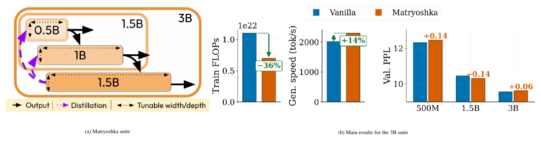
@floatnoticebox[b!] @noticestring end@float The way training and inference costs of large language models (LLMs) scale steeply with model size creates a demand for models across a broad spectrum of sizes, from 100M ([1]) to trillion ([2]) parameters, for diverse deployment scenarios. Delivering models from different scales allows for different load/performance tradeoffs, with smaller models being more memory- and compute-efficient than their larger counterparts. As a result, models are usually released in suites: groups of models trained separately on similar data, with smaller models often distilled from larger ones in the suite. The question of efficiency in training and serving model suites jointly is rarely studied. We propose a training framework that is particularly well-suited to the model-suite paradigm and offers several concrete benefits over the standard approach.

Instead of training separate models, our approach progressively stacks the outputs of smaller sub-models as inputs to larger ones. For instance, rather than training a ${1\text{B}, , 8\text{B}, , 30\text{B}, , 70\text{B}}$ suite as four independent runs, our method trains a single architecture combining a $1$ B sub-model with additional $7$ B, $22$ B, and $40$ B parameter blocks, resulting in 70B trained parameters instead of 109B. Contrarily to previous work ([3]), each sub-model can be detached as a standalone language model, with its own depth and KV cache footprint, and served independently just like a regular checkpoint. This setup also makes distillation from the largest model to all smaller ones a natural by-product, as logits from all submodels are available during training. As a result, training the Matryoshka suite costs on the same order as training only the largest model alone, and delivers all $N$ sub-models in a single run, with cheap knowledge distillation.

At inference time, the nested structure further benefits speculative decoding ([4]): the draft model is nested in the verifier model, and both already share KV cache, eliminating the usual memory overhead of maintaining a separate draft model. Cross-model prediction agreement is also higher than in independently trained suites, directly increasing token acceptance rates.

We verify our approach by training a 3B-parameter Matryoshka suite with 500M, 1.5B, and 3B sub-models on 35B tokens from the FineWeb-Edu dataset. Our suite matches independently trained baselines on validation perplexity, out-of-domain perplexity, and benchmark performance while using 36% less total training compute. Moreover, the shared-weight structure and low-cost distillation substantially improves cross-model agreement and makes larger draft models practical for speculative decoding. We also conduct an extensive analysis of architectural design, and show the impact of width and depth configurations in Matryoshka suites, and that both the distillation loss and our model junction mechanism are crucial for the performance of smaller sub-models. We release trained checkpoints and a HuggingFace's transformers-compatible implementation[^1].

[^1]: Checkpoints & inference code: https://huggingface.co/nthngdy/matryoshka-3B

Overall, our contributions can be summarized as:

• We introduce Matryoshka Language Model Suites, a pretraining framework that nests sub-models of increasing width and depth into a single jointly trained architecture (Section 2);
• We derive a low-cost distillation objective that leverages the availability of all sub-model logits at every forward pass;
• We train a 3B-parameter Matryoshka suite and show it reaches near-parity (within 0.5 average points at every size) with independently trained baselines on standard benchmarks while using 36% less training compute (Section 3);
• We demonstrate that the shared-weight structure and low-cost distillation substantially improve cross-model agreement and make larger drafts practical for speculative decoding, where plain vanilla speculative decoding barely improves over autoregressive inference.
• We provide extensive ablations at smaller scale (50M/100M/200M suite) that provide insights for architectural hyperparameters and training objectives.

2. Method

Section Summary: The method creates a nested family of Transformer language models in which each smaller model is a strict subset of the parameters of the next larger one, with each sub-model allowed its own width and depth. A parameter-free junction rescales and concatenates representations so that the output of one sub-model can serve as input to the next, while a combined cross-entropy and distillation loss is computed for every exit; because a single forward pass through the largest model produces logits for all sub-models, the distillation signal incurs no extra cost. The same nesting also supports efficient speculative decoding, as any smaller model can act as a draft generator that shares weights and KV cache with its larger verifier.

We nest smaller models into larger ones, and allow different hidden sizes across models by implementing a simple junction mechanism. We then compute a cross-entropy loss and a largest-model distillation loss for each exit points, and use a convex combination of these as a single overall objective.

Modeling

A Transformer ([5]) language model maps an input sequence $x \in [1, V]^L$ to output representations $o_\theta(x) \in \mathbb{R}^{L \times D}$ via an input embedding $e_\theta$ and a stack of Transformer blocks $T_\theta$ of hidden dimension $D$. A linear LM head $W$ maps each position's representation $o_\theta(x)$ to logits $l \in \mathbb{R}^V$, and the parameters $(\theta, W)$ are trained to minimize the next-token prediction cross-entropy loss.[^2]

[^2]: We notationally distinguish the LM head parameters to simplify the definition of our Matryoshka suite.

A conventional suite of $M$ models uses $M$ independent parameter sets ${(\theta_m, W_m)}_{m=1}^M$. We instead enforce a strict nesting of parameters with the exception of the LM head:

$ \theta_1 \subset \theta_2 \subset \cdots \subset \theta_M = \theta. $

Each sub-model $T_{\theta_m}$ is a separate Transformer stack with its own hidden dimension (or width) $D_m$, number of layers (or depth) $n_m$, and a LM head $W_m$. We require strictly increasing hidden dimensions $D_1 \leq D_2 \leq \cdots \leq D_M$. Unlike standard early exiting, which assumes a fixed hidden dimension across exits, the Matryoshka design lets each sub-model use a width tailored to its size, giving more flexibility in the architectural design at every sub-model size compared to early-exit methods ([6]). Moreover, because $\theta_m \subset \theta_{m+1}$, running the full architecture produces all $M$ sub-model logits in a single forward pass while activating fewer parameters and writing less KV cache than $M$ independent forward passes, facilitating distillation during training and multi-model inference methods such as speculative decoding.

Inter-model Junction

The main modeling difficulty consists in passing the output $o^{m}\theta(x) \in \mathbb{R}^{D_m}$ of sub-model $T{\theta_m}$ as the input to sub-model $T_{\theta_{m{+}1}}$, which operates in $\mathbb{R}^{D_{m+1}}$ with $D_{m+1} \geq D_m$. We design a junction mechanism that does not introduce any additional parameters.

The most naive approach is to concatenate $o^{m}\theta(x)$ with a fresh embedding $e^{m+1}\theta(x) \in \mathbb{R}^{D_{m+1}-D_m}$ extending to the "new" dimensions that sub-model $m{+}1$ adds. However, this creates a magnitude mismatch: Transformer outputs typically have much larger norms than input embeddings, which destabilizes training in the low-index channels. We address this by rescaling $o^{m}\theta(x)$ so that its norm matches the norm of $e^{m+1}\theta(x)$ before the concatenation. Formally, given $o^{m}\theta(x)$ the output embedding coming from the $m$-th submodel and $e^{m+1}\theta(x)$ the input embedding of the $(m+1)$-th submodel, we build the $(m+1)$-th submodel output $o^{m+1}_\theta(x)$ as follows:

$ \begin{aligned}&\tilde{o}^{m}\theta(x) = o^{m}\theta(x)\cdot \dfrac{|e^{m+1}\theta(x)|2}{|o^{m}\theta(x)|2}\&o^{m+1}\theta(x) = T^{m+1}\theta!\left(\operatorname{concat}!\left(e^{m+1}\theta(x), ;\tilde{o}^{m}\theta(x) \right)\right);;.\end{aligned}\tag{1} $

The first $D_m$ channels of the input to $T^{m+1}\theta$ carry information from sub-model $m$, while the remaining $D{m+1} - D_m$ channels are freshly initialized, analogous to the input embedding of a standalone model. Each sub-model has a dedicated LM head $W^m_\theta \in \mathbb{R}^{V \times D_m}$ and is trained with its own cross-entropy loss $\mathcal{L}^m_{\mathrm{ce}}$. Both design choices matter empirically: dropping the norm rescaling, or zeroing out the fresh embedding, degrades downstream PPL across all sub-model sizes (Table 3).

Integrated Distillation

In classical suite training, distillation from the largest model into smaller ones ([7, 8]) requires either storing teacher logits offline or running the teacher in parallel during student training. Each option adds significant compute or storage cost. In a Matryoshka suite, every forward pass through $\theta_M$ already produces logits for all $M$ sub-models simultaneously, making online distillation from the largest sub-model to all smaller ones free.

Concretely, we add a distillation term to each sub-model $m < M$, defined as the cross-entropy between the teacher and student next-token distributions:

$ \mathcal{L}^{M \to m}_d =

• \sum_{v=1}^{V} \texttt{stop_grad}(\sigma(l^M_t)_v) , \log \sigma(l^m_t)_v,\tag{2} $

where $\sigma$ denotes the softmax. The total loss for sub-model $m$ is a convex combination:

$ \mathcal{L}^m = (1 - \alpha_d), \mathcal{L}^m_{\mathrm{ce}}

• \alpha_d, \mathcal{L}^{M \to m}_d,\tag{3} $

and the overall training objective sums over sub-models: $\mathcal{L} = \sum_{m=1}^M \mathcal{L}^m$. The distillation coefficient $\alpha_d \in [0, 1]$ controls the strength of the teacher signal. We study its effect in Appendix A. We observe that $\alpha_d$ should be set to lower values compared to offline setups.

Speculative Decoding

At inference time, any pair $(m, m')$ with $m < m'$ forms a natural draft-verifier pair for speculative decoding ([4]). Sub-model $m$ generates a draft sequence of $\gamma$ tokens, which sub-model $m'$ then verifies in a single forward pass. The Matryoshka structure is orthogonal to draft-acceleration techniques such as EAGLE ([9]) or MEDUSA ([10]), which can be applied on top to further speed up inference. What we explore here is the complementary benefit of weight and KV-cache sharing between draft and verifier, which makes larger and hence stronger draft models practical.

Two properties make Matryoshka suites particularly well-suited for this setup. Because $\theta_m \subset \theta_{m'}$, the verifier's first $n_1 + \cdots + n_m$ layers coincide with the draft model's layers. The KV cache computed during drafting is fully reused by the verifier for those shared layers; only the $n_{m+1} + \cdots + n_{m'}$ additional layers need to run. This eliminates the memory cost of maintaining a separate draft model. Draft-verifier alignment is higher than in independently trained suites of the same sizes, as we confirm in Section 3, which directly translates to a higher token acceptance rate.

Together, these two properties make non-tiny drafts practical. Standard speculative decoding favors draft models one or two orders of magnitude smaller than the verifier (e.g., 60M drafts for an 11B target ([4]), or 160M–1B drafts for 7B–70B Llama ([11, 9])); larger drafts typically do not amortize, since their drafting cost and KV cache footprint grow faster than their acceptance rate. We show in Section 3.2.3 that a 500M / 3B pair (1:6 size ratio) is already in the unfavorable regime, with speculative decoding degrading latency compared to plain autoregressive inference. Yet, the Matryoshka 500M / 3B pair turns the same configuration into a 20–40% speedup over its own standard decoding by sharing its KV cache and early layers.

3. Experiments

Section Summary: In the experiments, researchers trained a Matryoshka suite of three nested language models (500M, 1.5B, and 3B parameters) from scratch on 35 billion tokens, using a shared architecture with carefully chosen layer depths and widths to match the memory and compute costs of a traditional baseline suite of three independent models. They compared the two approaches on standard benchmarks, training dynamics, and inference speedups via speculative decoding, while running smaller-scale tests to tune design choices such as distillation strength and model dimensions. The Matryoshka design achieved the target footprints with 38% fewer total parameters overall.

3.1 Experimental Setup

Architecture

We train a Matryoshka suite from scratch with three nested sub-models totalling 3B parameters, and compare it to an equivalent traditional suite; configurations are summarized in Table 1. The main architectural design choice is how to allocate the width and depth to each sub-model while matching the target parameter count.[^3] We adopt a deployment-oriented viewpoint and aim to match both memory and compute footprints across suite types.

[^3]: Given a target parameter count, and using standard configurations for FFN layers ($D_m \rightarrow 4\cdot D_m \rightarrow D_m$), fixing the depth $n_m$ of each sub-model determines its width $D_m$.

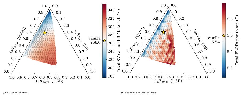
Because Matryoshka sub-models combine blocks of different widths, their compute and memory trade-offs differ from a uniform-width architecture, and the depth budget that balances per-token FLOPs and KV cache shifts accordingly. We use simple closed-form formulas for parameter count, KV cache, and per-token inference FLOPs (Appendix B). In our experiments, we use $L_v = 28$ layers for the standard 3B model and find $L = 39$ total layers to be the sweet spot for the 3B Matryoshka suite: shallower budgets (e.g. $L = 28$ matching the Vanilla baseline) reduce memory per token below the Vanilla footprint, while deeper ones (e.g. $L = 50$) inflate KV cache, with both mismatching the footprint of the Vanilla suite. Appendix C provides further discussion and analysis.

Within the $L = 39$ budget, we sweep all feasible depth triplets $(n_1, n_2, n_3)$ summing to 39, fixing target sizes (500M, 1.5B, 3B) and attention head dimensions (64, 96, 128), and for each triplet solve for the head count that best matches each target. Figure 2 reports the resulting KV cache and per-token FLOPs of the full 3B forward pass relative to a Vanilla 3B baseline. Our chosen configuration $(n_1, n_2, n_3) = (24, 10, 5)$ closely matches both KV cache and per-token FLOPs to the Vanilla 3B baseline. We notably choose to use the same width and depth for the 500M sub-model in both suites, to provide a strictly comparable data point. All sub-models share the SmolLM2 tokenizer ([1]) (49,152 tokens) and use RoPE ([12]) positional embeddings with $\theta_{\mathrm{RoPE}} = 10^5$.

\begin{tabular}{llrrrrrrr}
\toprule
  {} & & Params & Cumul. & $D_m$ & Layers & Heads & Head dim & Int. size \\
\midrule
\multirow{3}{*}{Vanilla}
   {} & 500M & \multicolumn{2}{c}{0.50B} & 1\, 024 & 24 & 16 & 64 & 4\, 096 \\
   {} & 1.5B & \multicolumn{2}{c}{1.51B} & 1\, 728 & 28 & 18 & 96 & 6\, 912 \\
   {} & 3B & \multicolumn{2}{c}{3.19B} & 2\, 560 & 28 & 20 & 128 & 10\, 240 \\
\midrule
\multirow{3}{*}{Matryoshka}
   {} & 500M & 0.50B & 0.50B & 1\, 024 & 24 & 16 & 64 & 4\, 096 \\
   {} & 1.5B & 0.98B & 1.48B & 2\, 304 & 10 & 24 & 96 & 9\, 216 \\
   {} & 3B & 1.72B & 3.20B & 4\, 352 & 5 & 34 & 128 & 17\, 408 \\
\bottomrule
\end{tabular}

Training Setup

Training uses 35B tokens from FineWeb-Edu ([13]), a high-quality education-focused web corpus, with sequences packed to length 2,048. The optimizer is AdamW with $(\beta_1, \beta_2) = (0.9, 0.95)$, $\epsilon = 10^{-8}$, peak learning rate 4 x 10^-4, weight decay $0.01$, and gradient clipping at $1.0$. We use a warmup-stable-decay (WSD) schedule with 3,000 cooldown steps over 33,000 total steps, a batch size of 512 sequences, and bf16 mixed precision. The distillation coefficient is set to $\alpha_d = 0.3$ for all main-suite runs, chosen from a smaller-scale proxy sweep (Appendix A). Combined training across both suites amounts to 52 GPU-days on NVIDIA B200.

As our primary baseline we train a Vanilla suite of three independent Llama-style ([14]) models at roughly the same sizes (0.50B, 1.51B, 3.19B; see Table 1), using the same tokenizer, data, and hyperparameters as the Matryoshka suite. Their shapes follow established small-LM conventions: the 500M and 1.5B Vanilla baselines mirror the SmolLM2 ([1]) configurations at those sizes, and the 3B Vanilla baseline follows the Llama-3.2-3B shape. Both suites are trained for 35B tokens; we additionally cool down and evaluate Vanilla checkpoints at 23B tokens to obtain a compute-matched reference.

3.2 Results and Analysis

We evaluate the Matryoshka suite against the Vanilla baseline along three axes: benchmark accuracy (Section 3.2.1), training dynamics and cross-model alignment (Section 3.2.2), and speculative decoding throughput (Section 3.2.3). Section 3.2.5 reports extensive ablations for widths and depths configurations, inter-model junction and loss coefficients at a smaller scale (50M/100M/200M parameters suite trained on 20B tokens).

3.2.1 Downstream Evaluation

We evaluate both suites zero-shot on seven multiple-choice benchmarks that are standard at this scale: ARC-Easy and ARC-Challenge ([15]), HellaSwag ([16]), LAMBADA ([17]), OpenBookQA ([18]), PIQA ([19]), and Winogrande ([20]). We also report average byte perplexity on five out-of-distribution corpora (WikiText-103 ([21]), C4 ([22]), PG-19 ([23]), arXiv, and PubMed); the per-corpus values are reported in Appendix F.

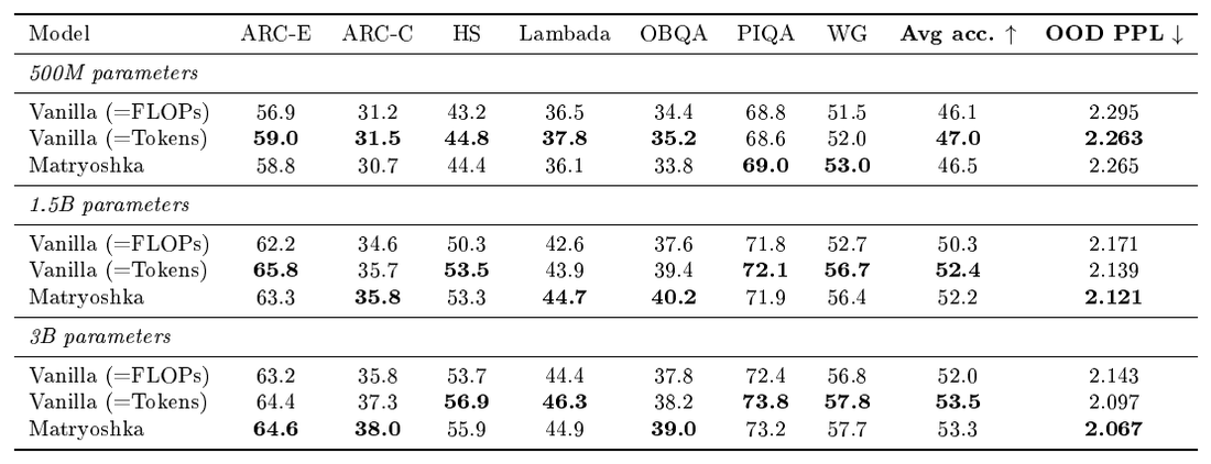
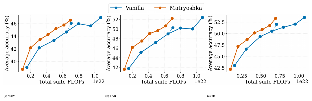
Table 2 shows that the Matryoshka suite reaches near-parity with the Token-matched Vanilla baseline on average accuracy at every size (within 0.5 points) while using 36% less training compute, and outperforms the FLOPs-matched Vanilla baseline at every size by +0.4 to +1.9 points. On average, OOD byte perplexity, the Matryoshka suite outperforms the Token-matched Vanilla baseline at the 1.5B and 3B scales (and ties at 500M), with the largest single-corpus advantage on arXiv (Appendix F). Figure 3 shows the same comparison as a function of total suite training FLOPs. The Matryoshka curve dominates the Vanilla curve at every compute level for every sub-model size.

::: {caption="Table 2: Per-benchmark accuracy and out-of-distribution perplexity. Vanilla (=FLOPs) uses the same 7.0e21 FLOPs as Matryoshka (23B tokens); Vanilla (=Tokens) uses the same 35B tokens at 57% more compute. Avg acc. averages the seven benchmarks (WG = Winogrande); OOD PPL averages WikiText-103, C4, PG-19, arXiv, and PubMed Central (Appendix F). Matryoshka reaches near-parity with Token-matched on accuracy and beats it on OOD PPL at 1.5B and 3B."}

:::

3.2.2 Training Dynamics and Model Agreement

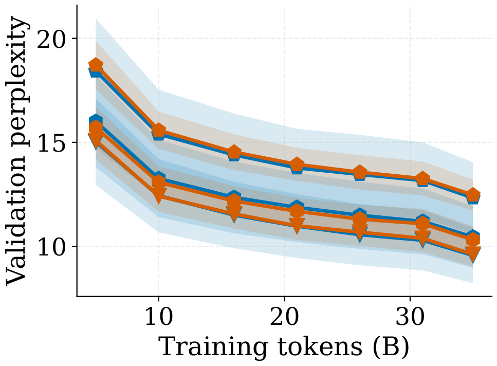
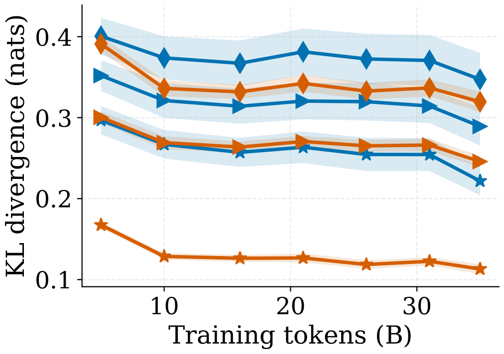
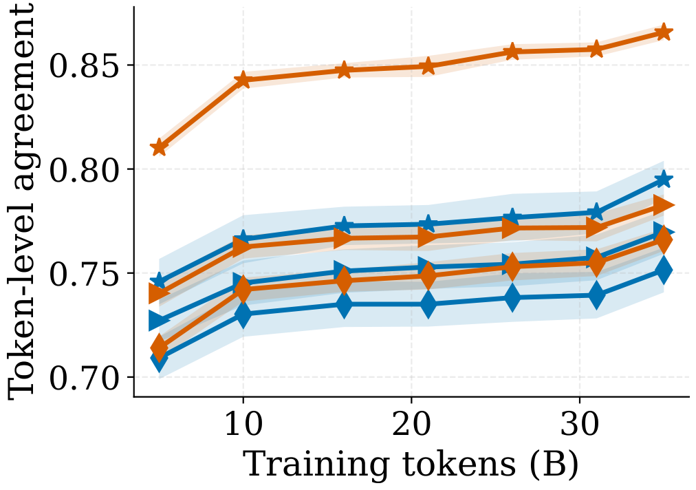
Figure 4 tracks validation perplexity, pairwise KL divergence, and pairwise top-1 next-token agreement throughout training. Matryoshka perplexity is on par with Vanilla perplexity at every checkpoint and every size (Figure 5); the parameter sharing and the junction mechanism do not harm language modeling quality. The small per-size gaps that remain are not intrinsic to the nested architecture: a proxy-scale sweep at 200M shows that simply rebalancing the per-sub-model loss weights, currently uniform in our recipe, closes a substantial fraction of the residual gap and shifts which size is the bottleneck (Appendix G).

A clear difference appears in cross-model alignment, as Matryoshka pairs exhibit noticeably lower KL divergence (Figure 6) and higher token-level agreement (Figure 7) than independently trained Vanilla pairs of matched sizes, with the effect strongest for the (1.5B, 3B) pair (+5.7% final agreement). This is a direct consequence of both the shared-weight structure and of online distillation across training. Independently trained models have no such constraint and develop different representations. The next-token agreement rate is the quantity that governs speculative decoding efficiency, which we discuss in Section 3.2.3.

3.2.3 Speculative Decoding Throughput

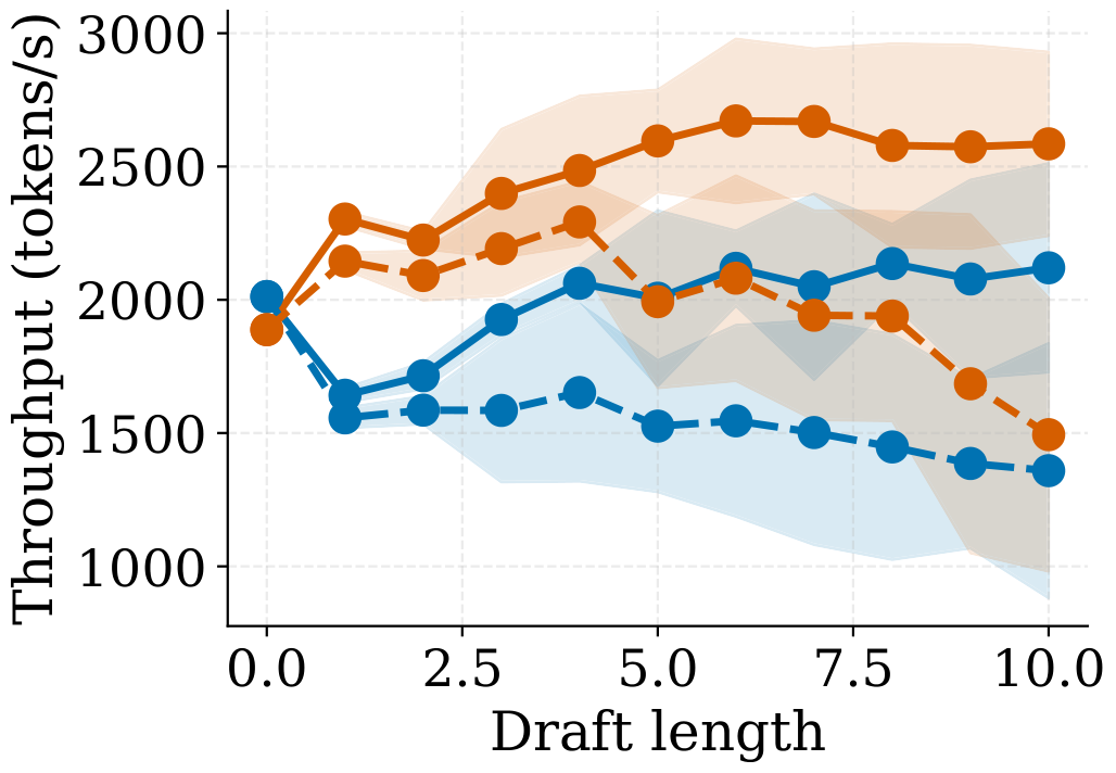
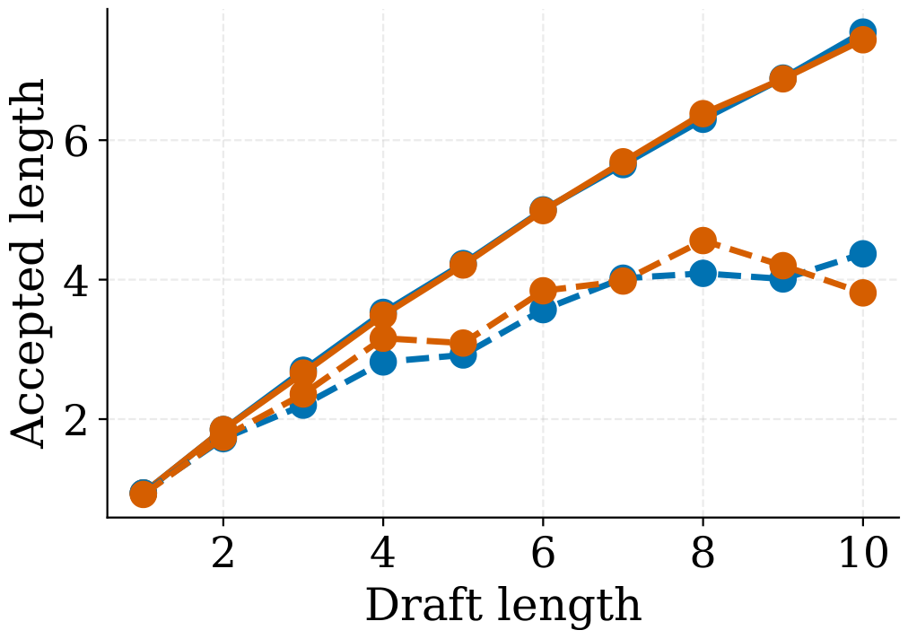
We measure speculative decoding throughput on an NVIDIA A100 GPU using the 500M sub-model as draft and the 3B sub-model as verifier, under both greedy and nucleus ($p=0.9$) sampling. The 500M / 3B size ratio (1:6) is large by literature standards, where draft models are typically one to two orders of magnitude smaller than the verifier ([4, 11, 9]). Each run uses prompts streamed from FineWeb-Edu truncated to 1,024 tokens, and generates 512 new tokens per prompt, sampled with temperature $0.4$. The maximum batch size that can fit the 80GB VRAM in such a setup is 64 for the Vanilla pair and 102 for the Matryoshka pair. The Matryoshka setup fits a larger batch in the same KV-cache budget thanks to the shared draft/verifier cache. A larger batch size allows for faster drafts relative to verification steps, as it reduces the bandwidth latency. Each metric is averaged over roughly 1M generated tokens.

Figure 8 shows that the Matryoshka pair achieves higher accepted length than the Vanilla pair across most draft lengths in the nucleus case (+5% in average), which directly reflects the agreement-rate gap in Figure 7. The higher acceptance translates to higher throughput: at a draft length of 6, Matryoshka reaches 2,650 tokens/s in greedy mode against 2,100 for Vanilla (a 26% speedup), and the gain is preserved under nucleus sampling. Crucially, the Vanilla 500M–3B pair barely beats plain autoregressive inference and is actually slower under nucleus sampling. At this size ratio, the draft-side KV cache and drafting FLOPs do not amortize against the acceptance rate.

3.2.4 Comparison with MatFormer

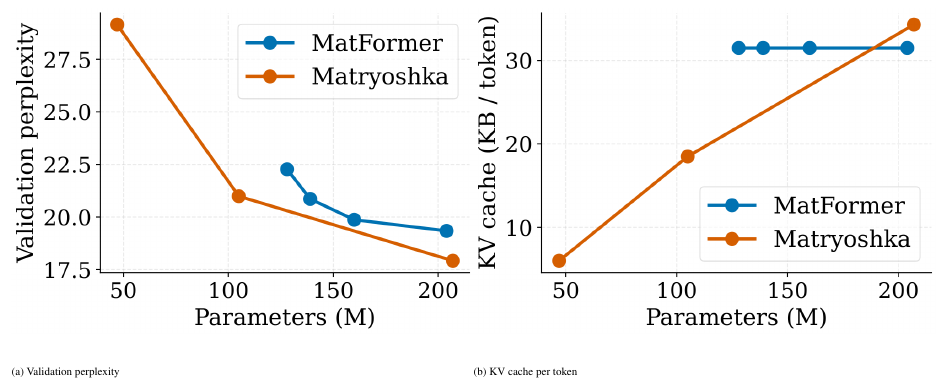
We compare our approach against MatFormer ([3]) at the 200M scale, training on 10B tokens, where both methods extract a suite of nested sub-models from a single training run (Figure 9). Because MatFormer nests along the FFN width while sharing a single attention backbone, all of its sub-models carry the same KV-cache footprint (31.5 KB/token), independent of their parameter count. In contrast, Matryoshka nests models along depth, so the KV cache shrinks together with the sub-model (down to 6.0 KB/token), yielding a genuinely lighter memory profile at inference time. We also observe a better quality–size trade-off: at matched validation perplexity ($\sim$ 21), Matryoshka-100M matches MatFormer-M (139M) with roughly half the KV cache and fewer parameters, and Matryoshka-200M attains both the lowest perplexity (17.92) of all compared models, including Matformer-XL (19.34).

3.2.5 Ablations

We ablate three design choices: the inter-model junction (with and without the norm-rescaling and the fresh embedding), the use of distillation (with and without), and the allocation of layers across sub-models. Our ablations are performed on a 200M proxy suite, composed of sub-models of 50M / 100M / 200M, where Matryoshka trades 41% less training compute for producing all three sub-models in a single run. Each full run for a 200M Matryoshka suite costs roughly five days of compute on a single A100 GPU, for 20B training tokens. Appendix A reports a separate sweep of the distillation coefficient $\alpha_d$.

Inter-model Junction

Recall that our recipe concatenates a fresh input embedding with a norm-rescaled model output. We compare it against two simpler alternatives in Table 3: concatenation without norm rescaling, and a zero junction that replaces the concatenated input embeddings with zeros. Our recipe matches the Vanilla baseline within 0.02 average PPL; removing the norm match introduces a +0.2 PPL gap, with a stronger impact on the smaller model; the zero junction is off on all model sizes, with a +0.54 PPL gap over our method. We also report the effect of removing distillation from the recipe, which causes a +0.15 PPL average gap more strongly noticeable on the smaller models. Both components are crucial for the performance of smaller sub-models.

\begin{tabular}{lrrrr}
\toprule
  {} & \multicolumn{4}{c}{Validation PPL $\downarrow$} \\
\cmidrule(lr){2-5}
Variant & 50M & 100M & 200M & Average \\
\midrule
Vanilla suite & 26.07 & 18.87 & 15.21 & 20.05 \\
\midrule
Zero padding & 26.98 & 18.83 & 16.01 & 20.61 \\
Input embs. + Distil. & 26.69 & 18.44 & 15.67 & 20.27 \\
Input embs. + Norm & 26.62 & 18.57 & \textbf{15.46} & 20.22 \\
Input embs. + Norm + Distil. (ours) & \textbf{26.16} & \textbf{18.43} & 15.62 & \textbf{20.07} \\
\bottomrule
\end{tabular}

Width/Depth of Sub-Models

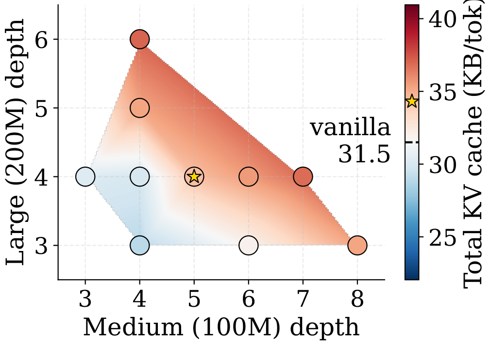
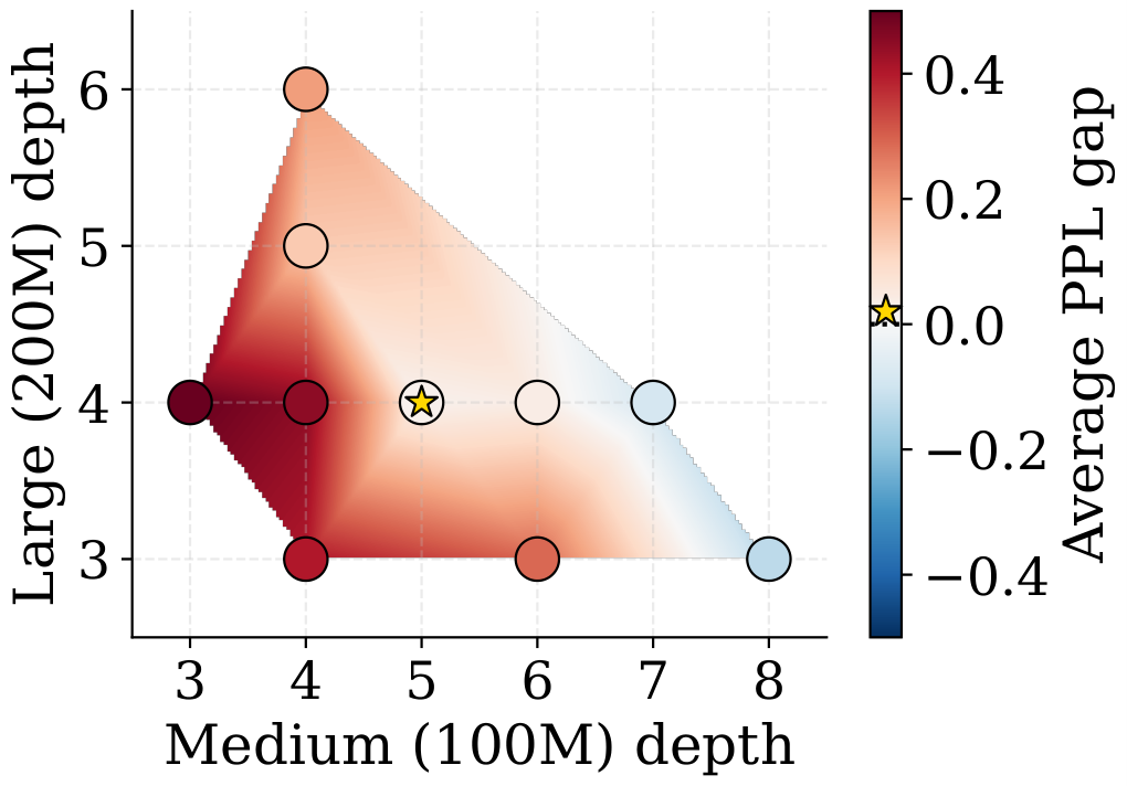
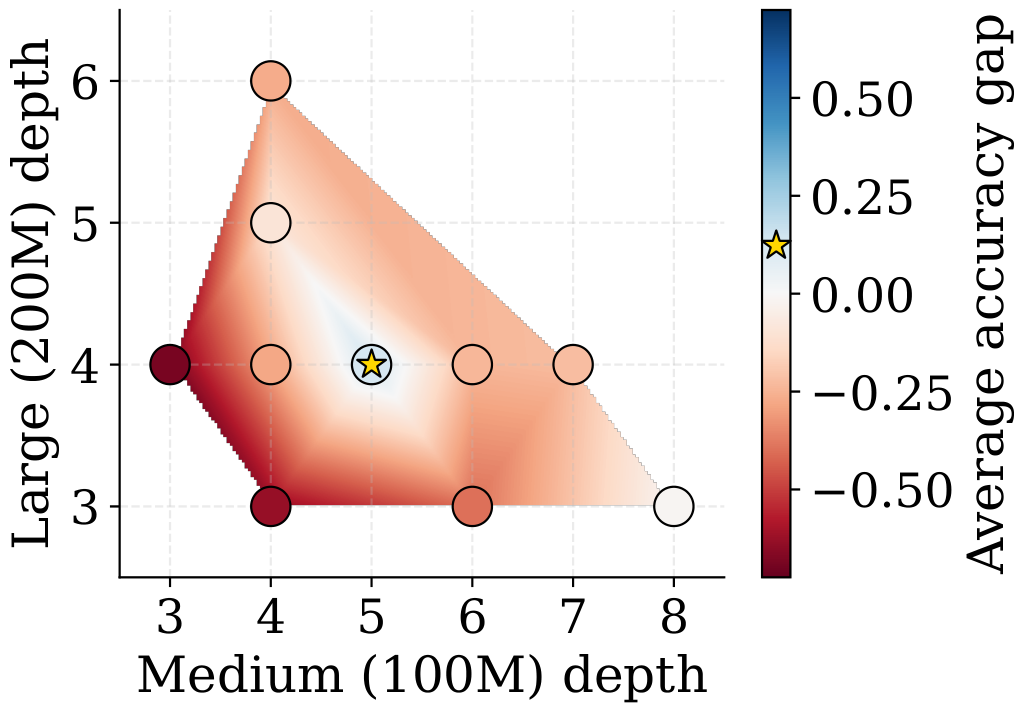
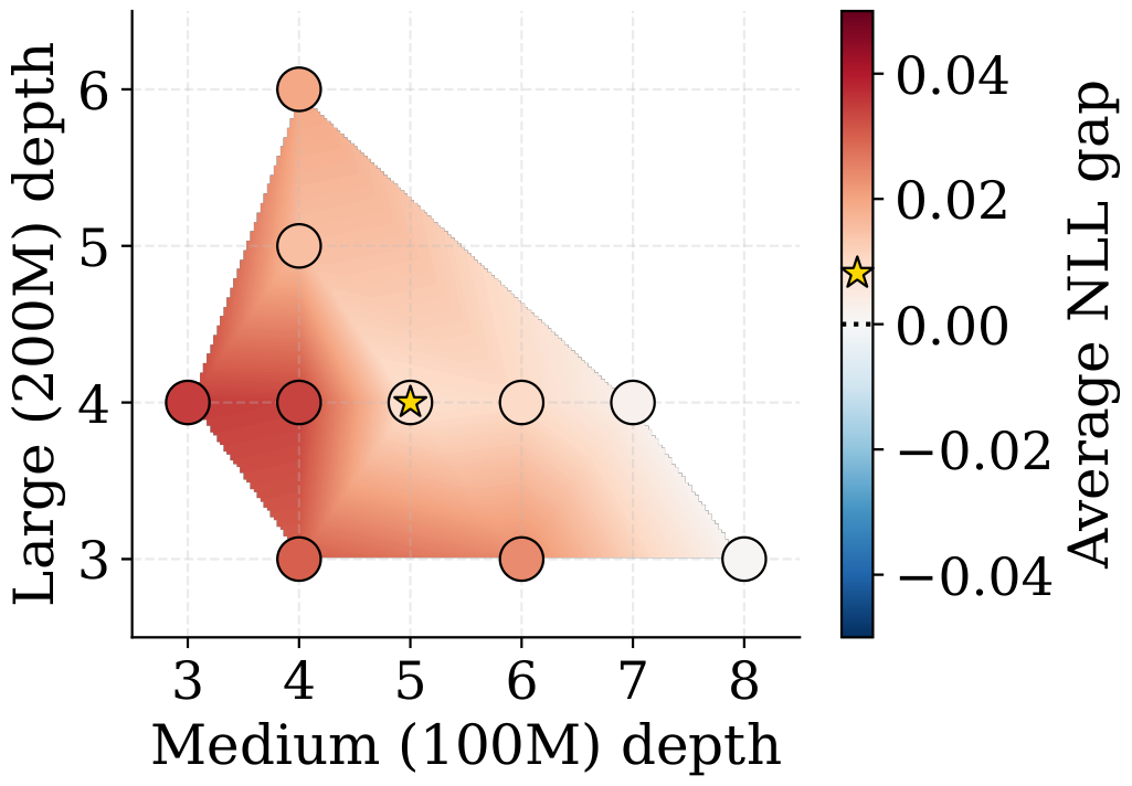
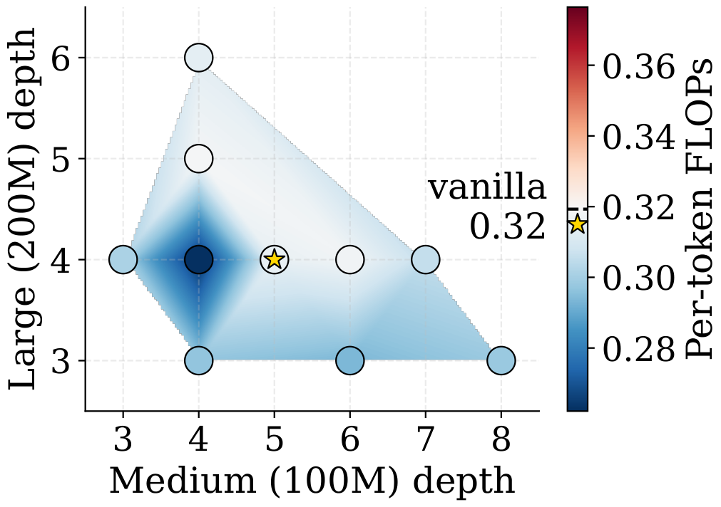
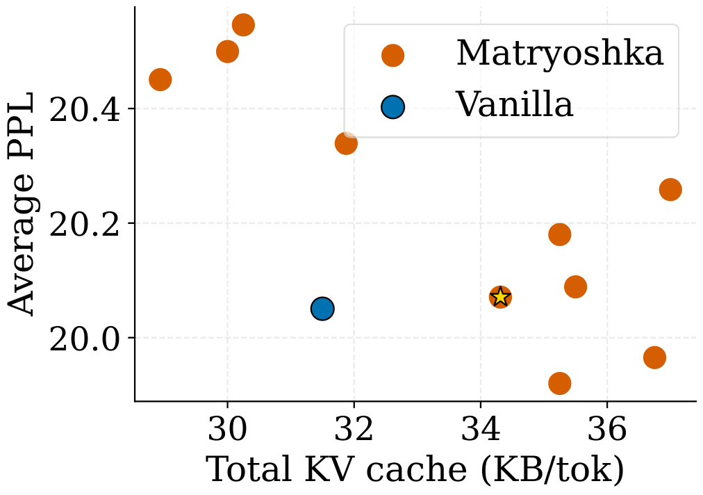
The depth triplet of the main 3B suite is one operating point in a rather large design space, as we show in Figure 2. At 200M parameter scale, the feasible configuration space is much less dense, which allows more coarse exploration. We sweep ten variants at the 200M scale that differ only in the depth split between the 100M and 200M blocks (Figure 11). The depth of each sub-model is then fixed to match the parameter size as closely as possible (within 5% in practice). In Figure 11, we observe that several variants are comparable to the vanilla suite both in terms of total KV cache growth and of average performance gap: the chosen $(L_1, L_2) = (5, 4)$ shape (gold star) remains within ${\sim}10%$ of the KV cache footprint of the Vanilla baseline at very low average PPL cost, and other variants achieve a further KV reduction with comparable PPL. Additional views (mean $\Delta\text{NLL}$, per-token FLOPs, 1D KV-cache summary) are reported in Appendix H. We also select the 200M variant with the lowest average PPL gap to the Vanilla baseline and report its downstream benchmark accuracy in Appendix I, where the same near-parity pattern as in the 3B suite holds.

4. Related Work

Section Summary: This section reviews prior techniques for making large language models more efficient at inference and training time. It covers early-exiting methods that stop computation once the model is confident, speculative decoding that uses a small draft model to propose tokens for a larger verifier to accept or reject, and elastic compression approaches that derive smaller models from an already-trained network. It then contrasts these with earlier Matryoshka-style work such as MatFormer, noting that the present framework nests sub-models in both width and depth to produce independent, deployable checkpoints with different memory and compute profiles.

Early Exiting

Early exiting makes predictions at intermediate layers to avoid a full forward pass when the model is already confident ([24]). In language modeling, this idea was applied by [25] and [26], and more recently via sparse layer routing by [27]. [6] combine layer dropout during pretraining with early-exit inference and self-speculative decoding from the early-exit layers. All these methods operate within a fixed-width architecture, whereas our sub-models differ in both width and depth, giving more flexibility in the accuracy-compute trade-off at each exit point. Furthermore, in Matryoshka suites there is no ambiguity about where to exit: exits correspond to fully trained sub-models with their own LM heads, not intermediate classifier probes.

Speculative Decoding and Distillation

Speculative decoding ([4]) accelerates autoregressive inference by letting a small draft model propose candidate continuations that a larger verifier accepts or rejects in parallel. The key efficiency lever is the token acceptance rate, which increases when draft and verifier are well aligned. [11] show that distilling the verifier into the draft model is a principled way to improve alignment. [28] combine speculative decoding with layer skipping for self-speculative decoding. In the Matryoshka framework, the verifier contains the Transformer stack of the draft model which is a form of static self-speculative decoding, and distillation from the largest sub-model to all smaller ones is a natural by-product of every training step, with negligible additional cost. More recently, the EAGLE line of work ([9, 29, 30]) trains lightweight feature-level draft heads on top of the verifier's penultimate representations, achieving 3–5 $\times$ speedups. [10] instead attach multiple parallel decoding heads to a single model to generate several future tokens at once. These methods are orthogonal to our work and could hypothetically be applied directly to our models and further adapted in our nested framework. Regarding pretraining-time distillation more broadly, [7] explore the design space of loss functions and teacher-student configurations, and [8] show that offline teacher logits reduce data requirements by $2.4\times$. Our approach alleviates the need for offline distillation by drastically reducing the cost of online distillation.

Elastic Compression of Pretrained LLMs

A line of work converts an existing trained LLM into a family of smaller models via elastic continued training, including Flextron ([31]), LLaMaFlex ([32]), and Nemotron Elastic ([33]). These methods build on the supernet lineage of slimmable networks ([34, 35]) and Once-for-All ([36]), and are complementary to our setting: they recover a family cheaply given a sunk pretraining cost, whereas we target the from-scratch suite-training problem.

Matryoshka LLMs

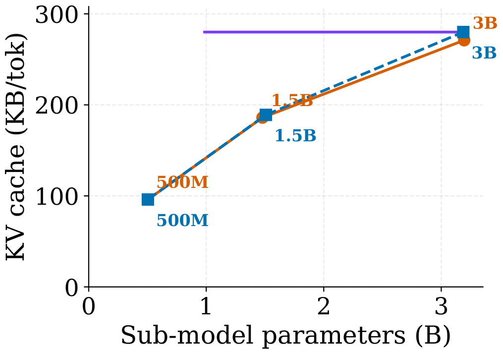
[37] introduce Matryoshka Representation Learning, where embedding prefixes of any length are trained to be informative. [3] apply the same principle to Transformers via MatFormer, nesting sub-models by varying the FFN hidden size across $g$ granularities while keeping depth, attention heads, and embeddings fixed. This yields FLOPs and parameter savings but leaves the KV-cache footprint per token identical across all sub-models, since every granularity inherits the parent's full attention configuration. Sub-models also are not independently deployable checkpoints. MatFormer thus targets a latency dial within a single deployment regime, rather than a suite spanning various target regimes with constrained memory usage and detachable per-size checkpoints. Our framework nests both width and depth, and produces standalone checkpoints, at the cost of a discrete rather than combinatorial set of sizes. Appendix E quantifies this contrast: at a fixed 3B universal shape, MatFormer's extractable sub-models sit above 1.05B parameters and share a constant $280$ KB/tok KV cache, whereas Matryoshka tracks the Vanilla curve down to a $500$ M sub-model with $96$ KB/tok of KV cache.

5. Conclusion

Section Summary: The paper introduces Matryoshka Language Model Suites, a nested pretraining approach that trains multiple model sizes together in one architecture to cut compute costs compared with training them independently. At the 3B scale this method nearly matches standard baselines while using 36% less training compute, and it also enables cheaper online distillation plus faster speculative decoding without extra memory use. The work points toward future research on jointly designing model suites and understanding how they combine with later instruction tuning or alignment steps.

We introduce Matryoshka Language Model Suites, a pretraining framework that stacks sub-models of increasing size into a single nested architecture trained end-to-end. The key insight is that the natural structure of a model suite, a set of models sharing the same training distribution, can be exploited by nesting at lower cost than independent training. At the 3B scale, our Matryoshka suite reaches near-parity with independently trained baselines on standard benchmarks while using 36% less training compute, allowing low-cost online distillation and enabling speculative decoding with higher throughput and no memory overhead for the draft model. Our ablations produce a solid basis for scaling up Matryoshka suites to larger sizes.

Our work paves the way for a new line of research on joint pretraining of model suites, where sub-models of different sizes are co-designed rather than trained in isolation. Open questions include how the recipe scales with more sub-models and larger budgets, how to allocate capacity and loss weight across sub-models, and how nested suites interact with post-training stages such as instruction tuning, alignment, and reasoning-oriented finetuning.

Acknowledgments

This work is partially supported by the National Science Foundation NSF under award OAC-2311521 and NASA under award No. 20-OSTFL20-0053. NG is supported by an Empire AI Postdoctoral Fellowship. We gratefully acknowledge use of the research computing resources of the Empire AI Consortium, Inc, with support from the State of New York, the Simons Foundation, and the Secunda Family Foundation ([38]). We would like to gratefully acknowledge the generous support of the NVIDIA Academic Grant Program. This work was supported as part of the “Swiss AI initiative” by a grant from the Swiss National Supercomputing Centre (CSCS) under project ID a0137 on Alps.

Appendix

Section Summary: The appendix first examines how varying the strength of a distillation signal affects sub-model quality on a small proxy suite, finding that a moderate coefficient best improves the smallest models without degrading larger ones and is therefore adopted for the main experiments. It then provides the exact formulas used to calculate parameter counts, KV-cache memory, per-token inference FLOPs, and overall training compute for both standard and nested Matryoshka architectures, incorporating hardware throughput measurements. Finally, it describes how the total layer budget was selected by balancing the computational and memory costs imposed by the largest sub-model.

A. Distillation Ablation

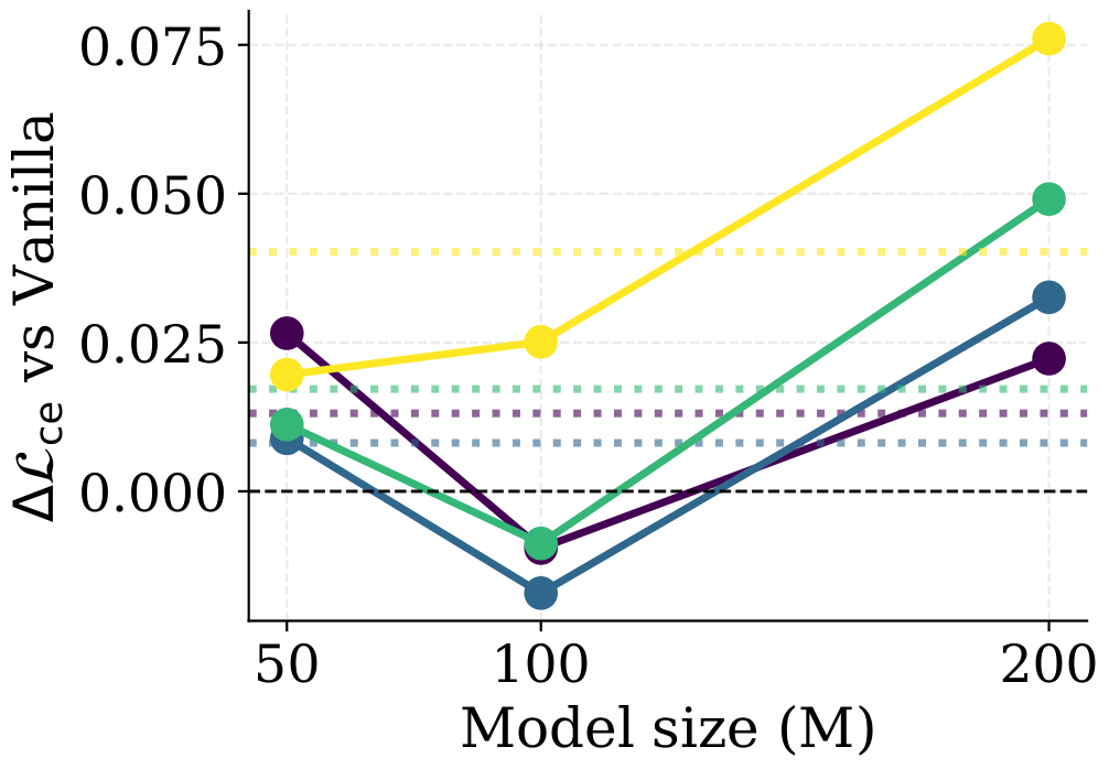
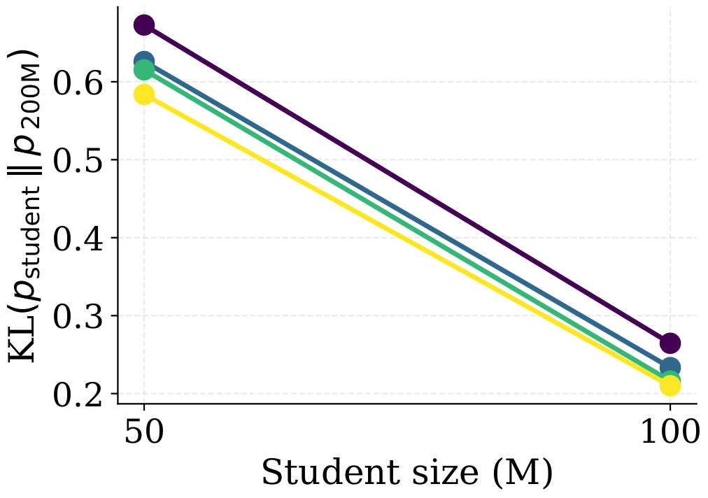
We sweep the distillation coefficient $\alpha_d \in {0, 0.3, 0.5, 0.7}$ on the 200M proxy suite (sub-models 50M / 100M / 200M, otherwise identical recipe to the main runs). Figure 10(a) reports the validation cross-entropy of each Matryoshka sub-model relative to its Vanilla-baseline counterpart; Figure 10(b) reports the KL divergence of each smaller sub-model to the 200M teacher, which captures how aligned each student becomes with the teacher under each setting.

In Figure 10(a), $\alpha_d = 0$ (no distillation) leaves the 50M and 200M sub-models above Vanilla while the intermediate 100M sub-model already sits below it; turning on the distillation signal ($\alpha_d = 0.3$) closes most of the 50M gap and pushes the average gap to its minimum across the four settings. Pushing $\alpha_d$ higher is counter-productive: at $\alpha_d = 0.5$ the largest sub-model starts trailing Vanilla, and $\alpha_d = 0.7$ degrades every size. The pattern in Figure 10(b) mirrors this — KL drops monotonically with $\alpha_d$, confirming that larger coefficients pull the student distribution closer to the teacher's, but at a cost on absolute language modeling quality once the cross-entropy term is too downweighted. We therefore use $\alpha_d = 0.3$ for the main 3B suite.

B. Compute, Memory, and Training-FLOPs Accounting

This appendix details the formulas used throughout the paper to report parameter counts, KV cache footprint, theoretical inference FLOPs, and training FLOPs. We use the following notation: $V$ is the vocabulary size, $L$ the number of Transformer layers, $H$ the hidden dimension (equal to the product of the number of attention heads and the head dimension), and $D$ the per-token training dataset size.

Parameter count

For a standalone Transformer with input embedding, $L$ blocks of width $D$ with $4D$ FFN intermediate dimension and an LM head, the total parameter count is

$ N_{\text{std}}(L, D) = 2 V D + 16 L D^2,\tag{4} $

where $2VD$ accounts for the input embedding and the LM head and $16 L D^2$ accounts for the per-layer cost (4 $D^2$ for self-attention projections and 12 $D^2$ for the FFN). For a Matryoshka suite of $M$ nested sub-models with shapes $(n_m, D_m)_{m=1}^M$, $D_1 \leq \cdots \leq D_M$, the cumulative parameter count observed at sub-model $m$ is

$ N^{\text{cumul}}m = 2 V D_m + \sum{j \le m} 16 , n_j D_j^2,\tag{5} $

where the $2 V D_m$ term reflects that sub-model $m$ uses the full input embedding at width $D_m$ together with its own LM head $W^m_\theta$. The total trainable parameter count of the suite further adds the LM heads of the smaller sub-models, $\sum_{m < M} V D_m$.

KV Cache

For a single decoded token at full attention, each Transformer layer stores both keys and values of width $D$, giving

$ \text{KV}(L, D) = 2 , b , L , D \quad \text{bytes per token},\tag{6} $

with $b$ bytes per element ($b = 2$ for bf16).

Theoretical Inference FLOPs

Counting two FLOPs per multiply-accumulate, the per-token forward-pass FLOPs of a standalone Transformer stack of width $D$ and depth $L$ is

$ F_{\text{stack}}(L, D) = 2 \cdot 16 , L D^2 = 32 , L D^2,\tag{7} $

to which we add a single LM head application of $2 V H$ FLOPs to produce the next-token logits. For the full Matryoshka suite, the per-token inference cost is the sum of the stack costs across all sub-models plus a single LM head at the deepest exit:

$ F^{\text{Mat}}{\text{infer}} = \sum{m=1}^M F_{\text{stack}}(n_m, D_m)

• 2 V D_M.\tag{8} $

The values reported in Figure 2 and elsewhere use these formulas directly.

Training FLOPs

We report training FLOPs by combining wall-clock GPU-hours with the nominal BF16 Tensor-Core peak of the GPU used for the run:

$ F_{\text{train}} = \frac{D}{(\text{tokens/GPU-hour})} \times 3600 \times F_{\text{peak}}^{\text{bf16}},\tag{9} $

where $D$ is the number of training tokens, the tokens-per-GPU-hour throughput is measured from training logs, and $F_{\text{peak}}^{\text{bf16}}$ is the GPU's nominal BF16 throughput (we use 4.5 x 10^15 FLOP/s for an NVIDIA B200 and 3.12 x 10^14 FLOP/s for an NVIDIA A100). This convention conflates the model's algorithmic FLOPs with hardware utilization, but it is the most faithful comparison between Vanilla and Matryoshka training costs, as any kernel-level differences are reflected in the measured throughput. Per-suite training FLOPs are the sum of $F_{\text{train}}$ over the runs that compose the suite (one joint run for Matryoshka, three independent runs for Vanilla).

C. Choice of Total Layer Budget

The Matryoshka suite assigns a depth $n_i$ to each sub-model under a fixed total budget $L = n_1 + n_2 + n_3$. Before searching the depth allocation inside $L$ (Figure 2), we first fix $L$ itself. The choice is constrained by two architectural costs of the 3B sub-model: per-token FLOPs and total KV cache. The Matryoshka 3B sub-model uses every layer across the three blocks, so $L$ directly determines its KV-cache footprint and, together with the per-block widths, its FLOPs.

To make the trade-off concrete, we sweep $L \in {28, 39, 50}$. For each $L$, we randomly sample roughly 500 valid depth allocations $(n_1, n_2, n_3)$ summing to $L$, and for each allocation we solve for the per-block widths that hit the (500M, 1.5B, 3B) parameter targets at fixed head dimensions $(64, 96, 128)$. We compute the resulting per-token FLOPs and total KV cache (in bf16) of the full 3B forward pass. Figure 11 plots each sample as a point colored by $L$; the black star marks the Vanilla 3B baseline (28 layers, $D_m = 2, 560$).

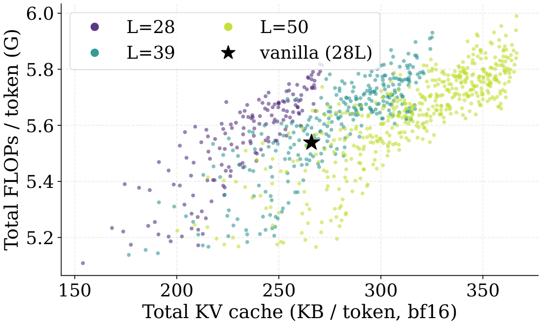
The three clouds occupy overlapping but distinct regions: $L = 28$ clusters at the lowest KV cache, but its FLOPs cloud sits mostly above the Vanilla baseline, because matching the 3B parameter target with only 28 shared layers forces wider matrices and higher FLOPs; $L = 50$ reaches the lowest FLOPs but pays a steep KV-cache cost (${\sim}25{-}40%$ above Vanilla), since KV cache scales linearly with depth and is unaffected by the FLOPs-saving width reduction; $L = 39$ contains allocations that simultaneously match or beat Vanilla on both axes — the only budget for which a strictly Pareto-dominant configuration exists. We therefore fix $L = 39$ as the depth budget and search inside it for the allocation $(n_1, n_2, n_3)$, which is the analysis reported in Figure 2.

Note that the impact of the width-depth ratio on LM quality is also studied in the literature ([39, 40, 41]), with the general finding that scale matters more than shape over a reasonable range of ratios. In the case of the Matryoshka models, matching the KV cache footprint matters for matching performance with a standard counterpart (Appendix H).

D. Reading the Ternary Plots

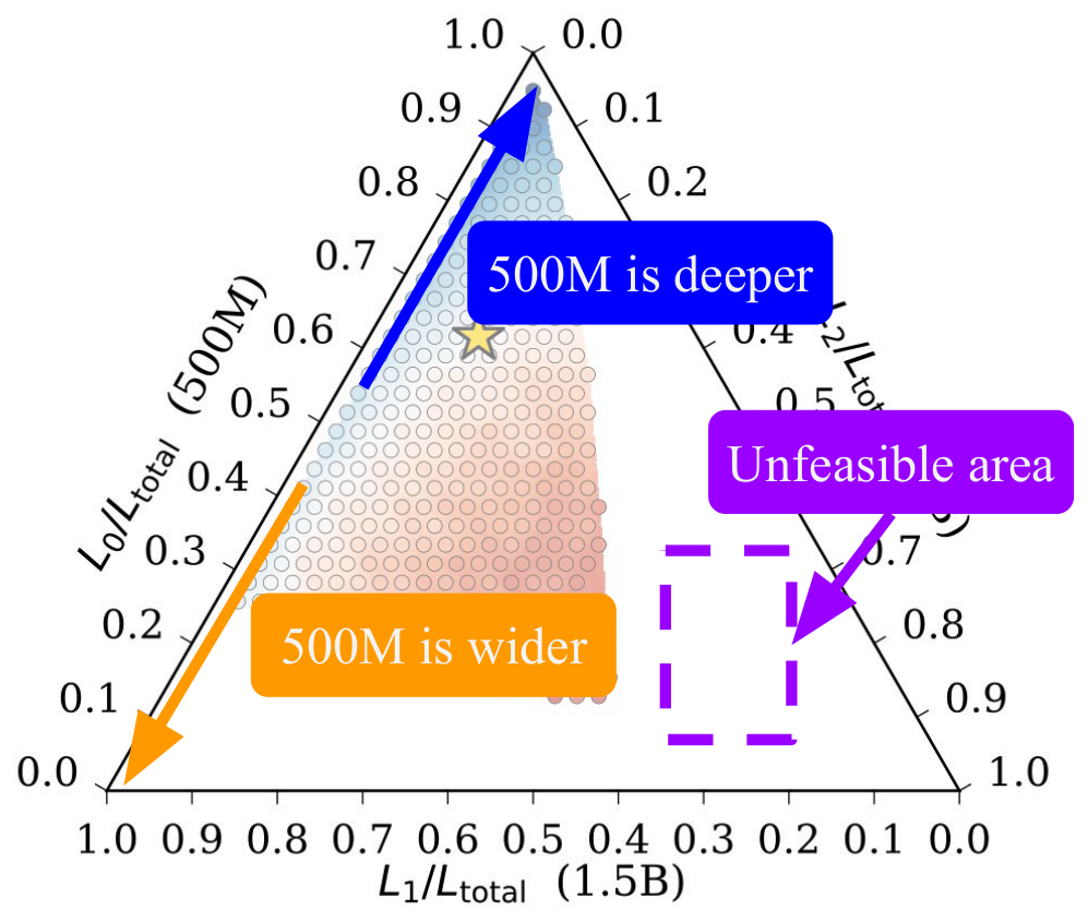
Several figures in this paper visualize the depth allocation $(L_0, L_1, L_2)$ across the three sub-models on a ternary diagram, with $L_0 + L_1 + L_2 = L_{\mathrm{total}}$ fixed. Each axis carries the fraction of total layers assigned to one sub-model, $L_i / L_{\mathrm{total}}$, so every point in the triangle corresponds to one valid normalized depth triplet. The three vertices represent the degenerate allocations where a single sub-model receives all layers; the three edges represent allocations where one sub-model receives zero layers. Figure 12 illustrates the conventions on the (500M, 1.5B, 3B) sweep at $L_{\mathrm{total}} = 39$.

Direction of motion has a concrete architectural meaning. Moving a point toward the top vertex increases $L_0 / L_{\mathrm{total}}$, the fraction of layers used by the 500M sub-model. To keep the 500M parameter target fixed, the per-layer width must shrink, so points near the top vertex correspond to a 500M sub-model that is deeper and narrower. Moving toward the bottom-left vertex decreases $L_0 / L_{\mathrm{total}}$ in favor of $L_1 / L_{\mathrm{total}}$ (the 1.5B share); the 500M sub-model then has fewer layers and must be wider to hit the same parameter count. The same logic applies to the other two axes. The gold star marks the configuration used in our main experiments, $(L_0, L_1, L_2) = (24, 10, 5)$.

The dashed region marked "unfeasible" contains depth triplets for which no valid Matryoshka architecture exists at the prescribed parameter targets. Concretely, given the head dimensions $(d_h^{(0)}, d_h^{(1)}, d_h^{(2)}) = (64, 96, 128)$ and target sizes (500M, 1.5B, 3B), we solve for the head count of each sub-model so that the cumulative parameter count matches the target. Two constraints can fail. Solving for the head count of a sub-model with too few layers can require fewer than one head, which is not realizable. More commonly, the nesting requirement $D_0 \leq D_1 \leq D_2$ on the hidden dimensions can be violated: when a larger sub-model is assigned too many layers, the only way to hit its parameter target is for it to be narrower than its predecessor, which is incompatible with the constraint. In both situations, this will lead to a missing point on the ternary graph.

E. Resource Comparison with MatFormer

To clarify how Matryoshka relates to other nested-architecture proposals, we compare it directly to MatFormer ([3]) on the two resource axes that matter at deployment time: KV cache footprint and per-token inference FLOPs. MatFormer applies its nesting only on the FFN block, leaving attention shape, hidden width, and depth fixed at the universal-model values. Sub-models are extracted by truncating the FFN intermediate dimension to a fraction $r \in (0, 4]$ of the universal $4 H$ width, with canonical granularities at $r \in {0.5, 1, 2, 4}$ in the original paper. Mix'n'Match supports any positive ratio in principle, so we sweep $r$ continuously below.

We fix the universal-model shape to the Vanilla 3B baseline (Table 1, $H = 2560$, $L = 28$) for both methods. For MatFormer we apply the standalone-Transformer formulas of Appendix B with FFN cost $3 r H^2$ per layer (three SwiGLU projections ([14]) of width $r H$). For Matryoshka we use the cumulative formulas at the three exit points (500M, 1.5B, 3B) of the 3B suite. Figure 13 reports the result.

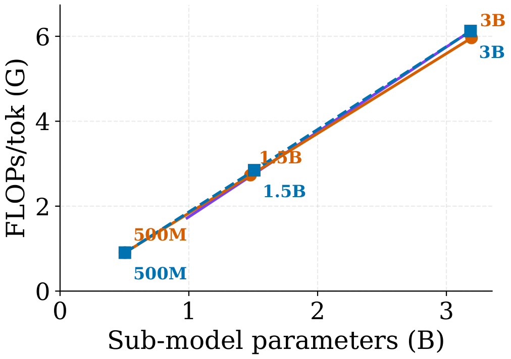
![Figure 13: Resource cost of extracting a sub-model from each framework, with the universal shape fixed to the Vanilla 3B baseline ($H = 2560$, $L = 28$). The MatFormer curve is a continuous sweep of FFN ratio $r \in (0, 4]$. Matryoshka and Vanilla are the three actual sub-models / independent baselines from Table 1. Lower-left is better on both panels.](img/legend_matformer.png)

Smallest Extractable Model Floor

The MatFormer trace in Figure 13 starts at roughly $1.26$ B parameters even at the smallest canonical granularity $r = 0.5$, and a hypothetical $r \to 0$ would still leave a $\sim$ 1.05B floor coming from the input embedding, the LM head, and the four attention projections at every layer, which are all kept at the universal width. This means a 3B universal MatFormer cannot expose a sub-500M extractable model at all, in either parameter count or FLOPs/tok: Figure 15 shows that MatFormer bottoms out at $2.27$ GFLOPs/tok, whereas Matryoshka and Vanilla both reach $0.91$ GFLOPs/tok at th e 500M exit. By contrast, Matryoshka places a 500M sub-model at the cumulative exit point of the smallest block, with parameter count, FLOPs, and KV cache all scaling down from there.

Matryoshka and KV Cache

On the FLOPs axis the three methods collapse onto essentially the same curve as a function of parameters, since FLOPs/tok is dominated by the same matrix-multiplication budget regardless of how the parameters are distributed across attention and FFN. KV cache, however, separates the methods cleanly. Figure 14 shows that MatFormer's KV cache is a horizontal line at $280$ KB/tok regardless of which sub-model is extracted, because attention shape and depth are fixed at the universal-model values. A deployment that needs a smaller KV footprint, e.g. to fit longer contexts or larger batches into the same memory budget, gains nothing from MatFormer's elasticity. Matryoshka instead reduces KV cache from $280$ KB to $96$ KB at the 500M exit, almost coincident with the $96$ KB of an independently trained Vanilla 500M model. Matryoshka thus matches the Vanilla curve on both axes across the full size range, confirming that the nested structure does not introduce inference-time overhead relative to a conventional suite, while delivering all sub-models from a single training run.

F. Out-of-Distribution Perplexity

To probe how well each suite generalizes outside FineWeb-Edu, we evaluate byte perplexity on five held-out corpora that span different domains: WikiText-103 (encyclopedic), C4 (general web), PG-19 (long-form fiction), arXiv (scientific full-text), and PubMed Central (biomedical full-text). All runs use a 2 048-token rolling window with stride 1 024 and the same SmolLM2 tokenizer. The Vanilla (FLOPs-matched) and Vanilla (Token-matched) baselines mirror those in Table 2. We report byte perplexity because it is invariant to tokenization differences and robust to long-tail vocabulary in PG-19, arXiv and PubMed.

Table 4 reports the per-corpus byte perplexity. The advantage is largest on arXiv, where the 3B Matryoshka sub-model lowers byte PPL by $0.13$ over the Token-matched Vanilla baseline; the 1.5B and 500M Matryoshka sub-models inherit part of this advantage through the shared early layers.

\begin{tabular}{lrrrrrr}
\toprule
Model & WikiText & C4 & PG-19 & arXiv & PubMed & \textbf{Average} \\
\midrule
\multicolumn{7}{l}{\textit{500M parameters}} \\
\midrule
Vanilla (FLOPs-matched) & 2.244 & 2.023 & 2.582 & 2.551 & 2.075 & 2.295 \\
Vanilla (Token-matched) & \textbf{2.215} & \textbf{2.003} & \textbf{2.504} & 2.530 & \textbf{2.065} & \textbf{2.263} \\
Matryoshka & 2.221 & 2.010 & 2.509 & \textbf{2.497} & 2.090 & 2.265 \\
\midrule
\multicolumn{7}{l}{\textit{1.5B parameters}} \\
\midrule
Vanilla (FLOPs-matched) & 2.138 & 1.953 & 2.361 & 2.454 & 1.951 & 2.171 \\
Vanilla (Token-matched) & 2.107 & 1.934 & 2.283 & 2.447 & \textbf{1.925} & 2.139 \\
Matryoshka & \textbf{2.100} & \textbf{1.931} & \textbf{2.228} & \textbf{2.398} & 1.946 & \textbf{2.121} \\
\midrule
\multicolumn{7}{l}{\textit{3B parameters}} \\
\midrule
Vanilla (FLOPs-matched) & 2.097 & 1.924 & 2.206 & 2.423 & 2.066 & 2.143 \\
Vanilla (Token-matched) & \textbf{2.059} & \textbf{1.906} & 2.129 & 2.442 & 1.950 & 2.097 \\
Matryoshka & 2.064 & \textbf{1.906} & \textbf{2.120} & \textbf{2.315} & \textbf{1.931} & \textbf{2.067} \\
\bottomrule
\end{tabular}

G. Closing the Per-Size Gap with Loss Weighting

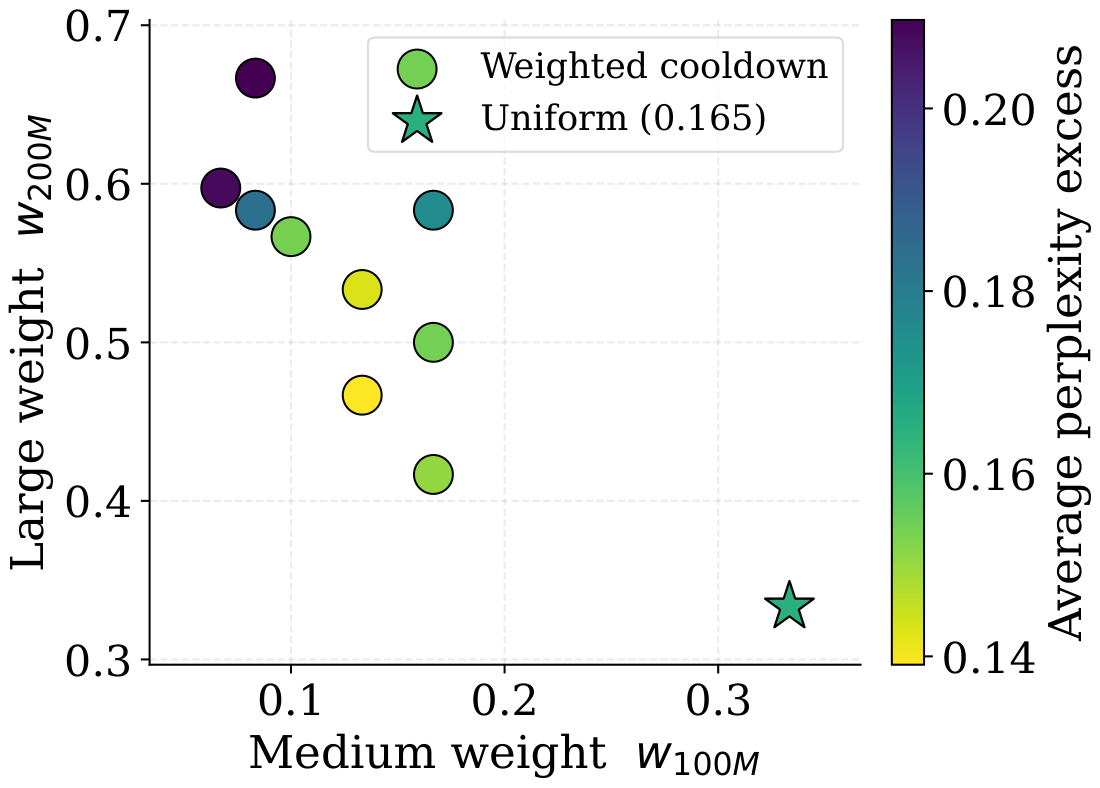
The default Matryoshka recipe weights each sub-model's loss equally in the total loss. This is a reasonable default but not necessarily optimal: the 50M, 100M, and 200M sub-models do not contribute equally to the gradient, and a uniform weighting over-serves some sizes at the expense of others. We probe whether the residual gap to Vanilla perplexity (Figure 5) can be closed by reweighting the per-sub-model losses, using the 200M proxy suite.

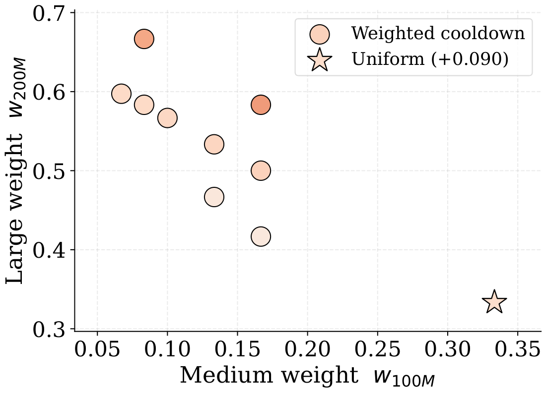
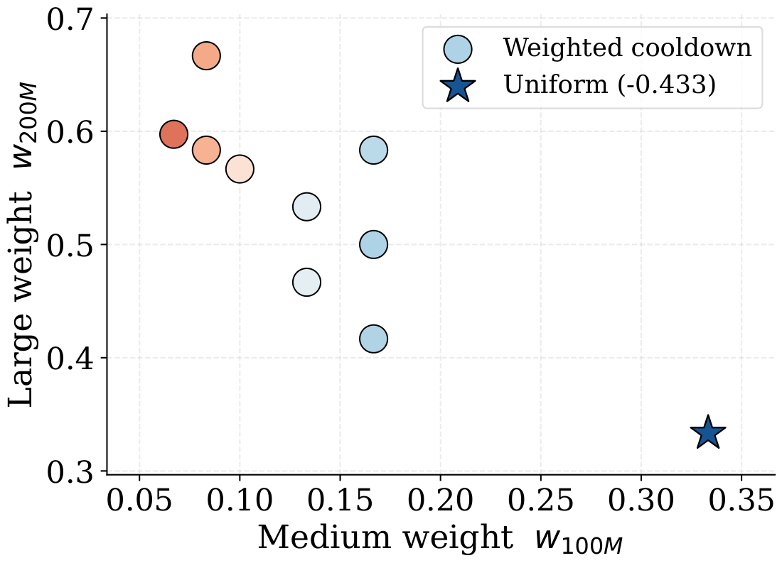
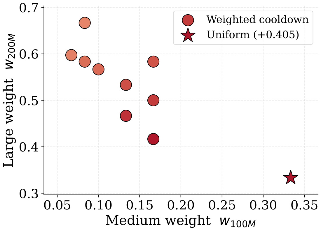
We sweep nine weight vectors $(w_{50}, w_{100}, w_{200})$ chosen to redistribute budget from sizes that are already at or below Vanilla toward those that remain above it; all vectors are normalized to sum to one. We re-run the last 1000 cooldown steps of the 200M Matryoshka run with each weighting, keeping the rest of the recipe identical. The reference is the uniform weighting $(1/3, 1/3, 1/3)$, which corresponds to the main recipe.

Figure 16 reports the average positive PPL excess of the weighted runs over Vanilla, defined as $\mathbb{E}{size}\left(, \max(0, , \mathrm{PPL}{Mat.}(size) - \mathrm{PPL}_{Van.}(size)) \right)$. This metric only penalizes sub-models that remain above Vanilla, so it captures how much negative gap remains rather than rewarding improvements for already-strong sub-models. Several weighted variants improve over uniform on this aggregate score, with the best configuration cutting the residual excess by roughly $15%$.

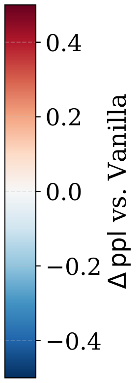
Figure 17 disaggregates the same runs by sub-model size. Each panel plots the per-size $\Delta\mathrm{PPL}$ over Vanilla as a function of $(w_{100}, w_{200})$ (with $w_{50} = 1 - w_{100} - w_{200}$ implicit). Two patterns are visible. First, under the uniform weighting (the star) the 100M sub-model is already substantially below Vanilla while the 200M sub-model is the bottleneck — equal weights over-serve 100M. Second, weightings that redistribute budget from $w_{100}$ toward $w_{200}$ (and mildly toward $w_{50}$) close the 200M gap and lift the 50M sub-model above Vanilla without breaking the 100M sub-model. No single weighting is Pareto-optimal on every axis, but several variants strictly dominate uniform on the aggregate score and on the bottleneck sub-model.

We did not extend this sweep to the 3B suite, because its compute cost is prohibitive and the qualitative finding is already useful at 200M. The takeaway is that part of the residual per-size gap to Vanilla in the main results is attributable to the uniform-weighting choice rather than to the nested architecture. This suggests that a simple, near-zero-cost hyperparameter tuning of $(w_m)$ would tighten the per-size results further; we leave a systematic per-size loss-weighting rule, including adaptive schedules, to future work.

H. Additional Size-and-Shape Ablation Views

Figure 11 reports two views of the 200M size-and-shape sweep: total KV cache per token and mean $\Delta\text{ppl}$ relative to a Vanilla baseline. In, we report three additional views: the mean $\Delta\text{NLL}$ counterpart of the perplexity scatter ((a)), the per-token theoretical-FLOPs scatter ((b)), and a 1D summary of mean NLL gap as a function of total KV cache ((c)). These views support the same conclusion as the main figure: the Matryoshka design space contains variants that simultaneously reduce KV cache and FLOPs relative to the Vanilla baseline without harming downstream quality.

As in Figure 11, each point is one Matryoshka variant with a shared 50M base sub-model, and $\Delta$ values are averaged over the three sub-model sizes (50M / 100M / 200M) versus the Vanilla 200M baseline of matching architecture.

I. 200M Proxy Suite Benchmarks

To complement the 3B-scale results, we evaluate the 200M proxy suite used throughout our ablations on the same downstream benchmarks as Table 2. The Vanilla baseline is the three independently trained 50M, 100M, and 200M models that share the recipe and tokenizer of the Matryoshka run; "Matryoshka" refers to our chosen v9 configuration. Both suites are trained for 20B tokens.

In Table 5, the Matryoshka suite ties Vanilla on the 50M sub-model ($-0.1$ avg) and beats it at 100M and 200M ($+0.4$ and $+0.1$ avg), confirming the perplexity parity reported in on downstream tasks.

\begin{tabular}{lccccccccc}
\toprule
Model & \multicolumn{1}{c}{ARC-E} & \multicolumn{1}{c}{ARC-C} & \multicolumn{1}{c}{HS} & \multicolumn{1}{c}{Lambada} & \multicolumn{1}{c}{OBQA} & \multicolumn{1}{c}{PIQA} & \multicolumn{1}{c}{WG} & \multicolumn{1}{c}{\textbf{Avg acc.} $\uparrow$} \\
\midrule
\multicolumn{9}{l}{\textit{50M parameters}} \\
\midrule
Vanilla & \textbf{44.2} & 23.6 & \textbf{28.5} & \textbf{17.5} & \textbf{29.4} & \textbf{60.1} & 50.2 & \textbf{36.2} \\
Matryoshka & 43.1 & \textbf{24.6} & 27.9 & 16.8 & 29.0 & 59.6 & \textbf{51.7} & 36.1 \\
\midrule
\multicolumn{9}{l}{\textit{100M parameters}} \\
\midrule
Vanilla & \textbf{47.4} & 25.4 & \textbf{32.3} & 24.1 & 31.0 & 62.1 & 51.5 & 39.1 \\
Matryoshka & 47.2 & \textbf{25.5} & 32.1 & \textbf{24.9} & \textbf{32.0} & \textbf{62.7} & \textbf{52.0} & \textbf{39.5} \\
\midrule
\multicolumn{9}{l}{\textit{200M parameters}} \\
\midrule
Vanilla & \textbf{51.8} & \textbf{27.7} & \textbf{36.7} & 29.4 & \textbf{33.2} & 64.5 & 50.8 & 42.0 \\
Matryoshka & 51.6 & 26.7 & 36.2 & \textbf{30.0} & 32.2 & \textbf{65.9} & \textbf{52.1} & \textbf{42.1} \\
\bottomrule
\end{tabular}

References

Section Summary: This references section compiles citations to academic papers, technical reports, and datasets that underpin research on efficient language models and AI inference methods. The listed works address topics such as transformer architectures, speculative decoding for faster text generation, knowledge distillation techniques, and benchmarks for evaluating reasoning and language understanding. They span foundational studies from 2017 through recent 2025–2026 advancements in model training and optimization.

[1] Loubna Ben Allal et al. (2025). SmolLM2: When Smol Goes Big – Data-Centric Training of a Small Language Model. https://arxiv.org/abs/2502.02737. arXiv:2502.02737.

[2] DeepSeek-AI (2026). DeepSeek-V4: Towards Highly Efficient Million-Token Context Intelligence. https://huggingface.co/deepseek-ai/DeepSeek-V4-Pro/blob/main/DeepSeek_V4.pdf.

[3] Fnu Devvrit et al. (2023). MatFormer: Nested Transformer for Elastic Inference. In Workshop on Advancing Neural Network Training: Computational Efficiency, Scalability, and Resource Optimization (WANT@NeurIPS 2023). https://openreview.net/forum?id=93BaEweoRg.

[4] Leviathan et al. (2023). Fast inference from transformers via speculative decoding. In Proceedings of the 40th International Conference on Machine Learning.

[5] Vaswani et al. (2017). Attention is All you Need. In Advances in Neural Information Processing Systems. pp. . https://proceedings.neurips.cc/paper_files/paper/2017/file/3f5ee243547dee91fbd053c1c4a845aa-Paper.pdf.

[6] Elhoushi et al. (2024). LayerSkip: Enabling Early Exit Inference and Self-Speculative Decoding. In Proceedings of the 62nd Annual Meeting of the Association for Computational Linguistics (Volume 1: Long Papers). pp. 12622–12642. doi:10.18653/v1/2024.acl-long.681. https://aclanthology.org/2024.acl-long.681/.

[7] Peng et al. (2025). Pre-training Distillation for Large Language Models: A Design Space Exploration. In Proceedings of the 63rd Annual Meeting of the Association for Computational Linguistics (Volume 1: Long Papers). pp. 3603–3618. doi:10.18653/v1/2025.acl-long.181. https://aclanthology.org/2025.acl-long.181/.

[8] Yuxian Gu et al. (2025). MiniPLM: Knowledge Distillation for Pre-training Language Models. In The Thirteenth International Conference on Learning Representations. https://openreview.net/forum?id=tJHDw8XfeC.

[9] Li et al. (2024). EAGLE: speculative sampling requires rethinking feature uncertainty. In Proceedings of the 41st International Conference on Machine Learning.

[10] Tianle Cai et al. (2024). Medusa: Simple LLM Inference Acceleration Framework with Multiple Decoding Heads. In Forty-first International Conference on Machine Learning. https://openreview.net/forum?id=PEpbUobfJv.

[11] Yongchao Zhou et al. (2024). DistillSpec: Improving Speculative Decoding via Knowledge Distillation. In The Twelfth International Conference on Learning Representations. https://openreview.net/forum?id=rsY6J3ZaTF.

[12] Su et al. (2024). RoFormer: Enhanced transformer with Rotary Position Embedding. Neurocomput.. 568(C). doi:10.1016/j.neucom.2023.127063. https://doi.org/10.1016/j.neucom.2023.127063.

[13] Guilherme Penedo et al. (2024). The FineWeb Datasets: Decanting the Web for the Finest Text Data at Scale. In The Thirty-eight Conference on Neural Information Processing Systems Datasets and Benchmarks Track. https://openreview.net/forum?id=n6SCkn2QaG.

[14] AI@Meta (2024). Llama 3 Model Card. https://github.com/meta-llama/llama3/blob/main/MODEL_CARD.md.

[15] Peter Clark et al. (2018). Think you have Solved Question Answering? Try ARC, the AI2 Reasoning Challenge. https://arxiv.org/abs/1803.05457. arXiv:1803.05457.

[16] Zellers et al. (2019). HellaSwag: Can a Machine Really Finish Your Sentence?. In Proceedings of the 57th Annual Meeting of the Association for Computational Linguistics. pp. 4791–4800. doi:10.18653/v1/P19-1472. https://aclanthology.org/P19-1472/.

[17] Paperno et al. (2016). The LAMBADA dataset: Word prediction requiring a broad discourse context. In Proceedings of the 54th Annual Meeting of the Association for Computational Linguistics (Volume 1: Long Papers). pp. 1525–1534. http://www.aclweb.org/anthology/P16-1144.

[18] Mihaylov et al. (2018). Can a Suit of Armor Conduct Electricity? A New Dataset for Open Book Question Answering. In Proceedings of the 2018 Conference on Empirical Methods in Natural Language Processing. pp. 2381–2391. doi:10.18653/v1/D18-1260. https://aclanthology.org/D18-1260/.

[19] Yonatan Bisk et al. (2020). PIQA: Reasoning about Physical Commonsense in Natural Language. In The Thirty-Fourth AAAI Conference on Artificial Intelligence, AAAI 2020, The Thirty-Second Innovative Applications of Artificial Intelligence Conference, IAAI 2020, The Tenth AAAI Symposium on Educational Advances in Artificial Intelligence, EAAI 2020, New York, NY, USA, February 7-12, 2020. pp. 7432–7439. doi:10.1609/AAAI.V34I05.6239. https://doi.org/10.1609/aaai.v34i05.6239.

[20] Sakaguchi et al. (2021). WinoGrande: an adversarial winograd schema challenge at scale. Commun. ACM. 64(9). pp. 99–106. doi:10.1145/3474381. https://doi.org/10.1145/3474381.

[21] Stephen Merity et al. (2017). Pointer Sentinel Mixture Models. In International Conference on Learning Representations. https://openreview.net/forum?id=Byj72udxe.

[22] Dodge et al. (2021). Documenting Large Webtext Corpora: A Case Study on the Colossal Clean Crawled Corpus. In Proceedings of the 2021 Conference on Empirical Methods in Natural Language Processing. pp. 1286–1305. doi:10.18653/v1/2021.emnlp-main.98. https://aclanthology.org/2021.emnlp-main.98/.

[23] Jack W. Rae et al. (2020). Compressive Transformers for Long-Range Sequence Modelling. In International Conference on Learning Representations. https://openreview.net/forum?id=SylKikSYDH.

[24] Surat Teerapittayanon et al. (2016). BranchyNet: Fast inference via early exiting from deep neural networks. 2016 23rd International Conference on Pattern Recognition (ICPR). pp. 2464-2469. https://api.semanticscholar.org/CorpusID:2916466.

[25] Schuster et al. (2022). Confident adaptive language modeling. Advances in Neural Information Processing Systems. 35. pp. 17456–17472.

[26] Maha Elbayad et al. (2020). Depth-Adaptive Transformer. In International Conference on Learning Representations. https://openreview.net/forum?id=SJg7KhVKPH.

[27] David Raposo et al. (2024). Mixture-of-Depths: Dynamically allocating compute in transformer-based language models. https://arxiv.org/abs/2404.02258. arXiv:2404.02258.

[28] Zhang et al. (2024). Draft & Verify: Lossless Large Language Model Acceleration via Self-Speculative Decoding. In Proceedings of the 62nd Annual Meeting of the Association for Computational Linguistics (Volume 1: Long Papers). pp. 11263–11282. doi:10.18653/v1/2024.acl-long.607. https://aclanthology.org/2024.acl-long.607/.

[29] Li et al. (2024). EAGLE-2: Faster Inference of Language Models with Dynamic Draft Trees. In Proceedings of the 2024 Conference on Empirical Methods in Natural Language Processing. pp. 7421–7432. doi:10.18653/v1/2024.emnlp-main.422. https://aclanthology.org/2024.emnlp-main.422/.

[30] Yuhui Li et al. (2026). EAGLE-3: Scaling up Inference Acceleration of Large Language Models via Training-Time Test. In The Thirty-ninth Annual Conference on Neural Information Processing Systems. https://openreview.net/forum?id=4exx1hUffq.

[31] Ruisi Cai et al. (2024). Flextron: Many-in-One Flexible Large Language Model. In Forty-first International Conference on Machine Learning. https://openreview.net/forum?id=9vKRhnflAs.

[32] Ruisi Cai et al. (2025). LLaMaFlex: Many-in-one LLMs via Generalized Pruning and Weight Sharing. In The Thirteenth International Conference on Learning Representations. https://openreview.net/forum?id=AyC4uxx2HW.

[33] Ali Taghibakhshi et al. (2025). Nemotron Elastic: Towards Efficient Many-in-One Reasoning LLMs. https://arxiv.org/abs/2511.16664. arXiv:2511.16664.

[34] Jiahui Yu et al. (2019). Slimmable Neural Networks. In International Conference on Learning Representations. https://openreview.net/forum?id=H1gMCsAqY7.

[35] Yu, Jiahui and Huang, Thomas (2019). Universally Slimmable Networks and Improved Training Techniques. In 2019 IEEE/CVF International Conference on Computer Vision (ICCV). pp. 1803-1811. doi:10.1109/ICCV.2019.00189. https://doi.ieeecomputersociety.org/10.1109/ICCV.2019.00189.

[36] Han Cai et al. (2020). Once-for-All: Train One Network and Specialize it for Efficient Deployment. In International Conference on Learning Representations. https://openreview.net/forum?id=HylxE1HKwS.

[37] Kusupati et al. (2022). Matryoshka Representation Learning.. In Advances in Neural Information Processing Systems.

[38] Bloom et al. (2025). Empire AI: A new model for provisioning AI and HPC for academic research in the public good. In Practice and Experience in Advanced Research Computing 2025: The Power of Collaboration. doi:10.1145/3708035.3736070. https://doi.org/10.1145/3708035.3736070.

[39] Jared Kaplan et al. (2020). Scaling Laws for Neural Language Models. https://arxiv.org/abs/2001.08361. arXiv:2001.08361.

[40] Tay et al. (2023). Scaling Laws vs Model Architectures: How does Inductive Bias Influence Scaling?. In Findings of the Association for Computational Linguistics: EMNLP 2023. pp. 12342–12364. doi:10.18653/v1/2023.findings-emnlp.825. https://aclanthology.org/2023.findings-emnlp.825/.

[41] Petty et al. (2024). The Impact of Depth on Compositional Generalization in Transformer Language Models. In Proceedings of the 2024 Conference of the North American Chapter of the Association for Computational Linguistics: Human Language Technologies (Volume 1: Long Papers). pp. 7239–7252. doi:10.18653/v1/2024.naacl-long.402. https://aclanthology.org/2024.naacl-long.402/.