Deep Learning Recommendation Model for Personalization and Recommendation Systems

Maxim Naumov, Dheevatsa Mudigere, Hao-Jun Michael Shi$^{*}$, Jianyu Huang,
Narayanan Sundaraman, Jongsoo Park, Xiaodong Wang, Udit Gupta$^{\dagger}$, Carole-Jean Wu,
Alisson G. Azzolini, Dmytro Dzhulgakov, Andrey Mallevich, Ilia Cherniavskii, Yinghai Lu,
Raghuraman Krishnamoorthi, Ansha Yu, Volodymyr Kondratenko, Stephanie Pereira,
Xianjie Chen, Wenlin Chen, Vijay Rao, Bill Jia, Liang Xiong and Misha Smelyanskiy
Facebook, 1 Hacker Way, Menlo Park, CA 94065
{mnaumov, dheevatsa}@fb.com

$^{*}$Northwestern University, $^{\dagger}$Harvard University, work done while at Facebook.

Abstract

With the advent of deep learning, neural network-based recommendation models have emerged as an important tool for tackling personalization and recommendation tasks. These networks differ significantly from other deep learning networks due to their need to handle categorical features and are not well studied or understood. In this paper, we develop a state-of-the-art deep learning recommendation model (DLRM) and provide its implementation in both PyTorch and Caffe2 frameworks. In addition, we design a specialized parallelization scheme utilizing model parallelism on the embedding tables to mitigate memory constraints while exploiting data parallelism to scale-out compute from the fully-connected layers. We compare DLRM against existing recommendation models and characterize its performance on the Big Basin AI platform, demonstrating its usefulness as a benchmark for future algorithmic experimentation and system co-design.

Executive Summary: The document introduces DLRM, a deep learning model for personalization and recommendation tasks such as ad click-through rate prediction. These systems are central to large internet platforms, yet neural network approaches that handle categorical features remain poorly understood compared with vision or language models, with training often taking weeks due to massive parameter counts.

The paper sets out to define a practical architecture that combines ideas from collaborative filtering and predictive modeling, to release working code, and to measure both accuracy and runtime behavior as a foundation for future benchmarks and hardware design.

The authors built DLRM by mapping categorical features to embedding tables and continuous features through a bottom multilayer perceptron, then explicitly computing pairwise dot-product interactions before a final top MLP produces a probability. They implemented the model in both PyTorch and Caffe2, applied model parallelism to the embeddings and data parallelism to the MLPs, and evaluated it on the public Criteo Kaggle and Terabyte datasets plus random and synthetic inputs. Experiments ran on the eight-GPU Big Basin server for one training epoch, with comparisons against a Deep & Cross network of similar size.

On the Kaggle dataset, DLRM reached slightly higher training and validation accuracy than the Deep & Cross baseline with either SGD or Adagrad, using roughly 540 million parameters in each case. Embedding lookups and fully connected layers dominate runtime; on CPUs the fully connected layers take the largest share, while on GPUs they become negligible. The model requires a custom all-to-all communication step between the bottom and top stages because of its mixed parallelism scheme.

These results show that a factorization-machine-style interaction pattern can deliver competitive accuracy at lower parameter cost than networks that build higher-order cross terms. The work also demonstrates that recommendation models have distinct scaling properties—primarily memory capacity and bandwidth for embeddings—different from those of CNNs or transformers, making them useful targets for system co-design.

The released implementations should be adopted as a public benchmark for algorithmic and hardware studies. Immediate next steps include profiling the custom communication layer, testing larger-scale multi-node runs, and exploring modest hyperparameter tuning or regularization to strengthen accuracy claims. Further work on optimized collective operations would reduce the current reliance on explicit copies.

The accuracy comparison rests on a single-epoch run without extensive tuning and on one public dataset; results on other production workloads could differ. The parallelism description is high-level, so quantitative scaling behavior remains to be reported. Overall, the architectural description and basic measurements are reliable, but readers should treat the performance numbers as preliminary reference points rather than definitive benchmarks.

1. Introduction

Section Summary: Personalization and recommendation systems at large internet companies, such as those predicting ad click rates, have recently shifted toward neural network designs after long use of other approaches. These designs draw on two lines of work: recommendation methods that progressed from expert-defined categories to collaborative filtering based on past user behavior and latent factors, and predictive models that moved from simple regression to deep networks using embeddings to handle categorical data. The paper introduces a deep learning recommendation model that merges these ideas by processing sparse and dense features through embeddings and neural layers, then explicitly interacting them to estimate event probabilities.

Personalization and recommendation systems are currently deployed for a variety of tasks at large internet companies, including ad click-through rate (CTR) prediction and rankings. Although these methods have had long histories, these approaches have only recently embraced neural networks. Two primary perspectives contributed towards the architectural design of deep learning models for personalization and recommendation.

The first comes from the view of recommendation systems. These systems initially employed content filtering where a set of experts classified products into categories, while users selected their preferred categories and were matched based on their preferences [1]. The field subsequently evolved to use collaborative filtering, where recommendations are based on past user behaviors, such as prior ratings given to products. Neighborhood methods [2] that provide recommendations by grouping users and products together and latent factor methods that characterize users and products by certain implicit factors via matrix factorization techniques [3, 4] were later deployed with success.

The second view comes from predictive analytics, which relies on statistical models to classify or predict the probability of events based on the given data [5]. Predictive models shifted from using simple models such as linear and logistic regression [6] to models that incorporate deep networks. In order to process categorical data, these models adopted the use of embeddings, which transform the one- and multi-hot vectors into dense representations in an abstract space [7]. This abstract space may be interpreted as the space of the latent factors found by recommendation systems.

In this paper, we introduce a personalization model that was conceived by the union of the two perspectives described above. The model uses embeddings to process sparse features that represent categorical data and a multilayer perceptron (MLP) to process dense features, then interacts these features explicitly using the statistical techniques proposed in [8]. Finally, it finds the event probability by post-processing the interactions with another MLP. We refer to this model as a deep learning recommendation model (DLRM); see Figure 1. A PyTorch and Caffe2 implementation of this model will be released for testing and experimentation with the publication of this manuscript.

2. Model Design and Architecture

Section Summary: The section describes the high-level architecture of DLRM by tracing its design to core building blocks from earlier recommendation systems. Embeddings convert sparse categorical inputs into dense vectors, which matrix factorization and factorization machines then combine via dot products or low-rank interactions to predict ratings or clicks, while multilayer perceptrons capture more complex nonlinear patterns. These pieces are assembled into a unified model that prioritizes both prediction quality and efficient computation on large-scale data.

In this section, we will describe the design of DLRM. We will begin with the high level components of the network and explain how and why they have been assembled together in a particular way, with implications for future model design, then characterize the low level operators and primitives that make up the model, with implications for future hardware and system design.

2.1 Components of DLRM

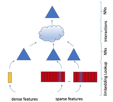
The high-level components of the DLRM can be more easily understood by reviewing early models. We will avoid the full scientific literature review and focus instead on the four techniques used in early models that can be interpreted as salient high-level components of the DLRM.

2.1.1 Embeddings

In order to handle categorical data, embeddings map each category to a dense representation in an abstract space. In particular, each embedding lookup may be interpreted as using a one-hot vector $\bm{e}_i$ (with the $i$-th position being $1$ while others are $0$, where index $i$ corresponds to $i$-th category) to obtain the corresponding row vector of the embedding table $W \in \mathbb{R}^{m \times d}$ as follows

$ \bm{w}_i^{T} = \bm{e}_i^{T} W . $

In more complex scenarios, an embedding can also represent a weighted combination of multiple items, with a multi-hot vector of weights $\bm{a}^T = [0, ..., a_{i_1}, ..., a_{i_k}, ..., 0]$, with elements $a_{i} \ne 0$ for $i = i_1, ..., i_k$ and $0$ everywhere else, where $i_1, ..., i_k$ index the corresponding items. Note that a mini-batch of $t$ embedding lookups can hence be written as

$ S = A^{T} W\tag{1} $

where sparse matrix $A = [\bm{a}_1, ..., \bm{a}_t]$ [7].

DLRMs will utilize embedding tables for mapping categorical features to dense representations. However, even after these embeddings are meaningfully devised, how are they to be exploited to produce accurate predictions? To answer this, we return to latent factor methods.

2.1.2 Matrix Factorization

Recall that in the typical formulation of the recommendation problem, we are given a set $\mathcal{S}$ of users that have rated some products. We would like to represent the $i$-th product by a vector $\bm{w}_i \in \mathbb{R}^d$ for $i = 1, ..., n$ and $j$-th user by a vector $\bm{v}_j \in \mathbb{R}^d$ for $j = 1, ..., m$ to find all the ratings, where $n$ and $m$ denote the total number of products and users, respectively. More rigorously, the set $\mathcal{S}$ consists of tuples $(i, j)$ indexing when the $i$-th product has been rated by the $j$-th user.

The matrix factorization approach solves this problem by minimizing

$ \min \sum_{(i, j) \in \mathcal{S}} r_{ij} - \bm{w}i^{T}\bm{v}{j}\tag{2} $

where $r_{ij} \in \mathbb{R}$ is the rating of the $i$-th product by the $j$-th user for $i = 1, ..., m$ and $j = 1, ..., n$. Then, letting $W^T=[\bm{w}_1, ..., \bm{w}_m]$ and $V^T=[\bm{v}_1, ..., \bm{v}n]$, we may approximate the full matrix of ratings $R=[r{ij}]$ as the matrix product $R \approx WV^T$. Note that $W$ and $V$ may be interpreted as two embedding tables, where each row represents a user/product in a latent factor space[^1] [4]. The dot product of these embedding vectors yields a meaningful prediction of the subsequent rating, a key observation to the design of factorization machines and DLRM.

[^1]: This problem is different from low-rank approximation, which can be solved by SVD [9], because not all entries of matrix $R$ are known.

2.1.3 Factorization Machine

In classification problems, we want to define a prediction function $\phi: \mathbb{R}^{n} \rightarrow T$ from an input datapoint $\bm{x} \in \mathbb{R}^{n}$ to a target label $y \in T$. As an example, we can predict the click-through rate by defining $T={+1, -1}$ with $+1$ denoting the presence of a click and $-1$ as the absence of a click.

Factorization machines (FM) incorporate second-order interactions into a linear model with categorical data by defining a model of the form

$ \hat{y} = b + \bm{w}^T\bm{x} + \bm{x}^T \texttt{upper}(VV^T)\bm{x}\tag{3} $

where $V \in \mathbb{R}^{n \times d}$, $\bm{w} \in \mathbb{R}^n$, and $b \in \mathbb{R}$ are the parameters with $d \ll n$, and upper selects the strictly upper triangular part of the matrix [8].

FMs are notably distinct from support vector machines (SVMs) with polynomial kernels [10] because they factorize the second-order interaction matrix into its latent factors (or embedding vectors) as in matrix factorization, which more effectively handles sparse data. This significantly reduces the complexity of the second-order interactions by only capturing interactions between pairs of distinct embedding vectors, yielding linear computational complexity.

2.1.4 Multilayer Perceptrons

Simultaneously, much recent success in machine learning has been due to the rise of deep learning. The most fundamental model of these is the multilayer perceptron (MLP), a prediction function composed of an interleaving sequence of fully connected (FC) layers and an activation function $\sigma : \mathbb{R} \rightarrow \mathbb{R}$ applied componentwise as shown below

$ \hat{y} = W_k \sigma(W_{k - 1} \sigma(... \sigma(W_1 \bm{x} + \bm{b}1) ...) + \bm{b}{k - 1}) + \bm{b}_k\tag{4} $

where weight matrix $W_l \in \mathbb{R}^{n_l \times n_{l - 1}}$, bias $\bm{b}_l \in \mathbb{R}^{n_l}$ for layer $l=1, ..., k$.

These methods have been used to capture more complex interactions. It has been shown, for example, that given enough parameters, MLPs with sufficient depth and width can fit data to arbitrary precision [11]. Variations of these methods have been widely used in various applications including computer vision and natural language processing. One specific case, Neural Collaborative Filtering (NCF) [12, 13] used as part of the MLPerf benchmark [14], uses an MLP rather than dot product to compute interactions between embeddings in matrix factorization.

2.2 DLRM Architecture

So far, we have described different models used in recommendation systems and predictive analytics. Let us now combine their intuitions to build a state-of-the-art personalization model.

Let the users and products be described by many continuous and categorical features. To process the categorical features, each categorical feature will be represented by an embedding vector of the same dimension, generalizing the concept of latent factors used in matrix factorization Equation 2. To handle the continuous features, the continuous features will be transformed by an MLP (which we call the bottom or dense MLP) which will yield a dense representation of the same length as the embedding vectors Equation 4.

We will compute second-order interaction of different features explicitly, following the intuition for handling sparse data provided in FMs Equation 3, optionally passing them through MLPs. This is done by taking the dot product between all pairs of embedding vectors and processed dense features. These dot products are concatenated with the original processed dense features and post-processed with another MLP (the top or output MLP) Equation 4, and fed into a sigmoid function to give a probability.

We refer to the resulting model as DLRM, shown in Figure 1. We show some of the operators used in DLRM in PyTorch [15] and Caffe2 [16] frameworks in Table 1.

: Table 1: DLRM operators by framework

	Embedding	MLP	Interactions	Loss
PyTorch	nn.EmbeddingBag	nn.Linear/addmm	matmul/bmm	nn.CrossEntropyLoss
Caffe2	SparseLengthSum	FC	BatchMatMul	CrossEntropy

2.3 Comparison with Prior Models

Many deep learning-based recommendation models [17, 18, 19, 20, 21, 22] use similar underlying ideas to generate higher-order terms to handle sparse features. Wide and Deep, Deep and Cross, DeepFM, and xDeepFM networks, for example, design specialized networks to systematically construct higher-order interactions. These networks then sum the results from both their specialized model and an MLP, passing this through a linear layer and sigmoid activation to yield a final probability. DLRM specifically interacts embeddings in a structured way that mimics factorization machines to significantly reduce the dimensionality of the model by only considering cross-terms produced by the dot-product between pairs of embeddings in the final MLP. We argue that higher-order interactions beyond second-order found in other networks may not necessarily be worth the additional computational/memory cost.

A key difference between DLRM and other networks is in how these networks treat embedded feature vectors and their cross-terms. In particular, DLRM (and xDeepFM [20]) interpret each feature vector as a single unit representing a single category, whereas networks like Deep and Cross treat each element in the feature vector as a new unit that should yield different cross-terms. Hence, Deep and Cross networks will produce cross-terms not only between elements from different feature vectors as in DLRM via the dot product, but also produce cross-terms between elements within the same feature vector, resulting in higher dimensionality.

3. Parallelism

Section Summary: Modern recommendation models contain enormous embedding tables that vastly exceed the memory of any single device, so these tables must be split across processors while the smaller multilayer-perceptron layers are replicated and updated on separate data batches. This hybrid scheme requires additional all-to-all exchanges so that every processor receives the embedding fragments it needs, plus collective reduction steps to keep the replicated layers consistent. Because existing frameworks lack native support for the combination, the authors implemented the required communication operators by hand.

Modern personalization and recommendation systems require large and complex models to capitalize on vast amounts of data. DLRMs particularly contain a very large number of parameters, up to multiple orders of magnitude more than other common deep learning models like convolutional neural networks (CNN), transformer and recurrent networks (RNN), and generative networks (GAN). This results in training times up to several weeks or more. Hence, it is important to parallelize these models efficiently in order to solve these problems at practical scales.

As described in the previous section, DLRMs process both categorical features (with embeddings) and continuous features (with the bottom MLP) in a coupled manner. Embeddings contribute the majority of the parameters, with several tables each requiring in excess of multiple GBs of memory, making DLRM memory-capacity and bandwidth intensive. The size of the embeddings makes it prohibitive to use data parallelism since it requires replicating large embeddings on every device. In many cases, this memory constraint necessitates the distribution of the model across multiple devices to be able satisfy memory capacity requirements.

On the other hand, the MLP parameters are smaller in memory but translate into sizeable amounts of compute. Hence, data-parallelism is preferred for MLPs since this enables concurrent processing of the samples on different devices and only requires communication when accumulating updates. Our parallelized DLRM will use a combination of model parallelism for the embeddings and data parallelism for the MLPs to mitigate the memory bottleneck produced by the embeddings while parallelizing the forward and backward propagations over the MLPs. Combined model and data parallelism is a unique requirement of DLRM as a result of its architecture and large model sizes. Such combined parallelism is not supported in either Caffe2 or PyTorch (as well as other popular deep learning frameworks), therefore we design a custom implementation. We plan to provide its detailed performance study in forthcoming work.

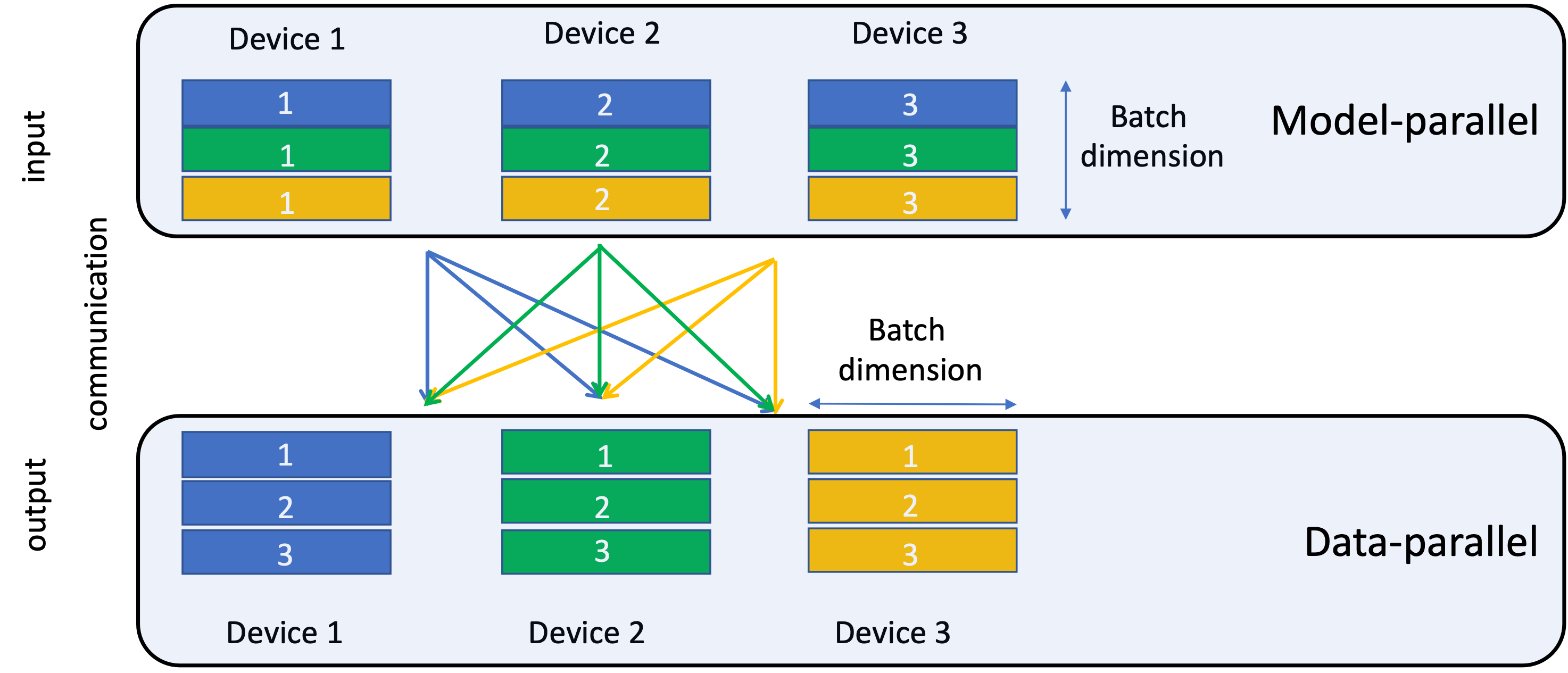
In our setup, the top MLP and the interaction operator require access to part of the mini-batch from the bottom MLP and all of the embeddings. Since model parallelism has been used to distribute the embeddings across devices, this requires a personalized all-to-all communication [23]. At the end of the embedding lookup, each device has a vector for the embedding tables resident on those devices for all the samples in the mini-batch, which needs to be split along the mini-batch dimension and communicated to the appropriate devices, as shown in Figure 2. Neither PyTorch nor Caffe2 provide native support for model parallelism; therefore, we have implemented it by explicitly mapping the embedding operators (nn.EmbeddingBag for PyTorch, SparseLengthSum for Caffe2) to different devices. Then personalized all-to-all communication is implemented using the butterfly shuffle operator, which appropriately slices the resulting embedding vectors and transfers them to the target devices. In the current version, these transfers are explicit copies, but we intend to further optimize this using the available communication primitives (such as all-gather and send-recv).

We note that for the data parallel MLPs, the parameter updates in the backward pass are accumulated with an allreduce[^2] and applied to the replicated parameters on each device [23] in a synchronous fashion, ensuring the updated parameters on each device are consistent before every iteration. In PyTorch, data parallelism is enabled through the nn.DistributedDataParallel and nn.DataParallel modules that replicate the model on each device and insert allreduce with the necessary dependencies. In Caffe2, we manually insert allreduce before the gradient update.

[^2]: Optimized implementations for the allreduce op. include Nvidia's NCCL [24] and Facebook's gloo [25].

4. Data

Section Summary: The section describes three kinds of data sets used to test and benchmark the model. Random data sets generate artificial continuous values and categorical indices on the fly, allowing hardware and systems experiments without relying on external storage. Synthetic data sets replicate statistical patterns from real traces to explore memory behavior or protect privacy, while public data sets such as the Criteo click logs enable accuracy measurements on genuine recommendation data.

In order to measure the accuracy of the model, test its overall performance, and characterize the individual operators, we need to create or obtain a data set for our implementation. Our current implementation of the model supplies three types of data sets: random, synthetic and public data sets.

The former two data sets are useful in experimenting with the model from the systems perspective. In particular, it permits us to exercise different hardware properties and bottlenecks by generating data on the fly while removing dependencies on data storage systems. The latter allows us to perform experiments on real data and measure the accuracy of the model.

4.1 Random

Recall that DLRM accepts continuous and categorical features as inputs. The former can be modeled by generating a vector of random numbers using either a uniform or normal (Gaussian) distributions with the numpy.random package rand or randn calls with default parameters. Then a mini-batch of inputs can be obtained by generating a matrix where each row corresponds to an element in the mini-batch.

To generate categorical features, we need to determine how many non-zero elements we would like have in a given multi-hot vector. The benchmark allows this number to be either fixed or random within a range[^3] $[1, k]$. Then, we generate the corresponding number of integer indices, within a range $[1, m]$, where $m$ is the number of rows in the embedding $W$ in Equation 1. Finally, in order to create a mini-batch of lookups, we concatenate the above indices and delineate each individual lookup with lengths (SparseLengthsSum) or offsets (nn.EmbeddingBag)[^4].

[^3]: see options --num-indices-per-lookup=k and --num-indices-per-lookup-fixed

[^4]: For instance, in order to represent three embedding lookups, with indices ${0, 2}$, ${0, 1, 5}$ and ${3}$ we use

$ \begin{aligned} \texttt{lengths/offsets} &=& {2, 3, 1} / {0, 2, 5} \nonumber \ \texttt{indices} &=& {0, 2, 0, 1, 5, 3} \nonumber \end{aligned} $

Note that this format resembles Compressed-Sparse Row (CSR) often used for sparse matrices in linear algebra.

4.2 Synthetic

There are many reasons to support custom generation of indices corresponding to categorical features. For instance, if our application uses a particular data set, but we would not like to share it for privacy purposes, then we may choose to express the categorical features through distributions. This could potentially serve as an alternative to the privacy preserving techniques used in applications such as federated learning [26, 27]. Also, if we would like to exercise system components, such as studying memory behavior, we may want to capture fundamental locality of accesses of original trace within synthetic trace.

Let us now illustrate how we can use a synthetic data set. Assume that we have a trace of indices that correspond to embedding lookups for a single categorical feature (and repeat the process for all features). We can record the unique accesses and frequency of distances between repeated accesses in this trace (Algorithm 1) and then generate a synthetic trace (Algorithm 2) as proposed in [28].

Let `tr` be input sequence, `s` stack of distances, `u` list of unique accesses and `p` probability distribution
Let `s.position(from)_the(top)` return d=0 if the index is not found, and d>0 otherwise.
**for** `i=0`; `i<length(tr)`; `i++` **do**
  `a = tr[i]`
  `d = s.position(from)_the(top)(a)`
  **if** `d == 0` **then**
    `u.append(a)`
  **else**
    `s.remove(from)_the(top)_at(position)(d)`
  **end if**
  `p[d]` += `1.0/length(tr)`
  `s.push(to)_the(top)(a)`
**end for**

Let `u` be input list of unique accesses and `p` probability distribution of distances, while `tr` output trace.
**for** `s=0`, `i=0`; `i<length`; `i++` **do**
  `d = p.sample(from)_distribution(with)_support(0,s)`
  **if** `d == 0` **then**
    `a = u.remove(from)_front()`
    `s++`
  **else**
    `a = u.remove(from)_the(back)_at(position)(d)`
  **end if**
  `u.append(a)`
  `tr[i] = a`
**end for**

Note that we can only generate a stack distance up to s number of unique accesses we have seen so far, therefore s is used to control the support of the distribution p in Algorithm 2. Given a fixed number of unique accesses, the longer input trace will result in lower probability being assigned to them in Algorithm 1, which will lead to longer time to achieve full distribution support in Algorithm 2. In order to address this problem, we increase the probability for the unique accesses up to a minimum threshold and adjust support to remove unique accesses from it once all have been seen. A visual comparison of probability distribution p based on original and synthetic traces is shown in Figure 3. In our experiments original and adjusted synthetic traces produce similar cache hit/miss rates.

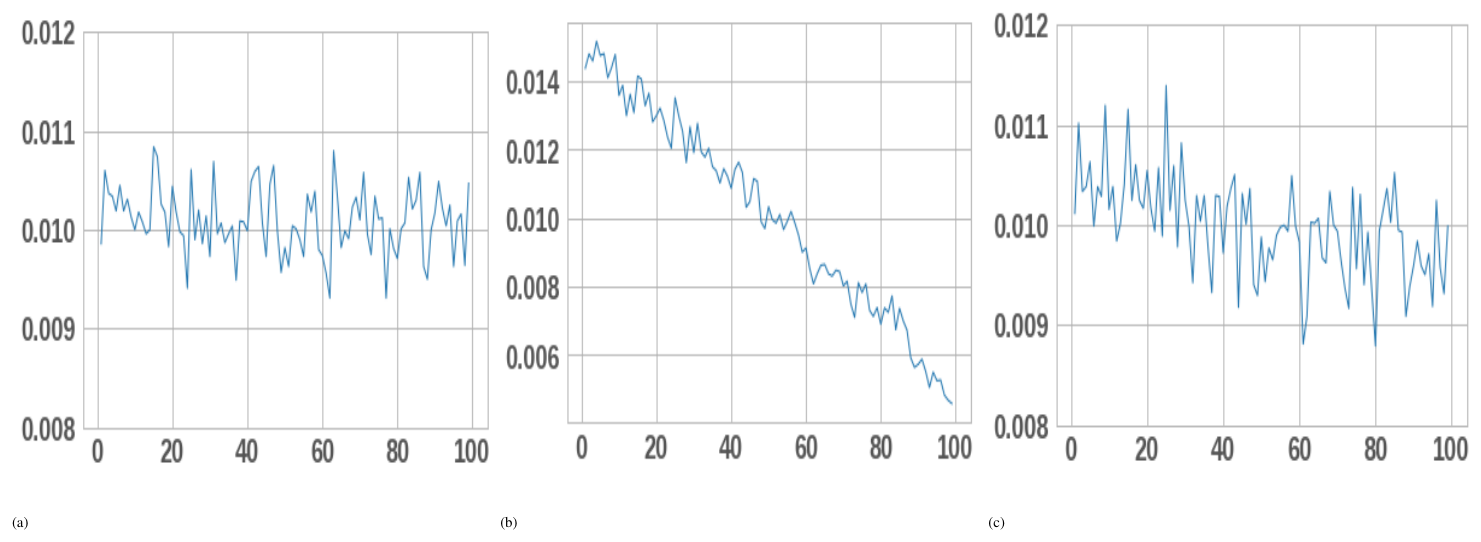
Algorithm 1 and Algorithm 2 were designed for more accurate cache simulations, but they illustrate a general idea of how probability distributions can be used to generate synthetic traces with desired properties.

4.3 Public

Few public data sets are available for recommendation and personalization systems. The Criteo AI Labs Ad Kaggle^5 and Terabyte^6 data sets are open-sourced data sets consisting of click logs for ad CTR prediction. Each data set contains 13 continuous and 26 categorical features. Typically the continuous features are pre-processed with a simple log transform $\log(1 + x)$. The categorical feature are mapped to its corresponding embedding index, with unlabeled categorical features or labels mapped to 0 or NULL.

The Criteo Ad Kaggle data set contains approximately 45 million samples over 7 days. In experiments, typically the 7th day is split into a validation and test set while the first 6 days are used as the training set. The Criteo Ad Terabyte data set is sampled over 24 days, where the 24th day is split into a validation and test set and the first 23 days is used as a training set. Note that there are an approximately equal number of samples from each day.

5. Experiments

Section Summary: The experiments evaluate the DLRM recommendation model, implemented in PyTorch and Caffe2, on servers equipped with Intel Xeon CPUs and Nvidia V100 GPUs. On the public Criteo advertising dataset, the model reached slightly higher training and validation accuracy than a comparable Deep and Cross Network while using a similar number of parameters. Separate profiling runs on a smaller synthetic model showed that the full workload completed in roughly one-quarter the time on a GPU versus a CPU, with embedding lookups and neural-network layers accounting for most runtime.

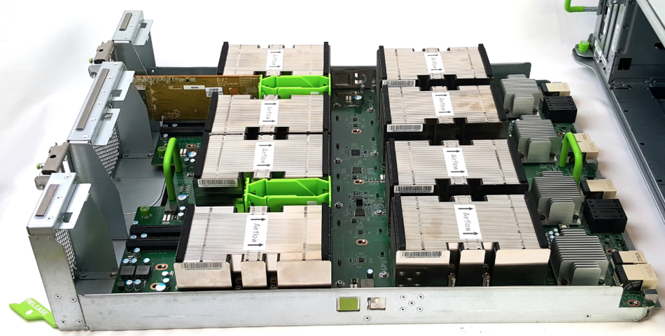
Let us now illustrate the performance and accuracy of DLRM. The model is implemented in PyTorch and Caffe2 frameworks and is available on GitHub^7. It uses fp32 floating point and int32(Caffe2)/int64(PyTorch) types for model parameters and indices, respectively. The experiments are performed on the Big Basin platform with Dual Socket Intel Xeon 6138 CPU @ 2.00GHz and eight Nvidia Tesla V100 16GB GPUs, publicly available through the Open Compute Project^8, shown in Figure 4.

5.1 Model Accuracy on Public Data Sets

We evaluate the accuracy of the model on Criteo Ad Kaggle data set and compare the performance of DLRM against a Deep and Cross network (DCN) as-is without extensive tuning [19]. We compare with DCN because it is one of the few models that has comprehensive results on the same data set. Notice that in this case the models are sized to accommodate the number of features present in the data set. In particular, DLRM consists of both a bottom MLP for processing dense features consisting of three hidden layers with $512$, $256$ and $64$ nodes, respectively, and a top MLP consisting of two hidden layers with $512$ and $256$ nodes. On the other hand DCN consists of six cross layers and a deep network with $512$ and $256$ nodes. An embedding dimension of $16$ is used. Note that this yields a DLRM and DCN both with approximately $540M$ parameters.

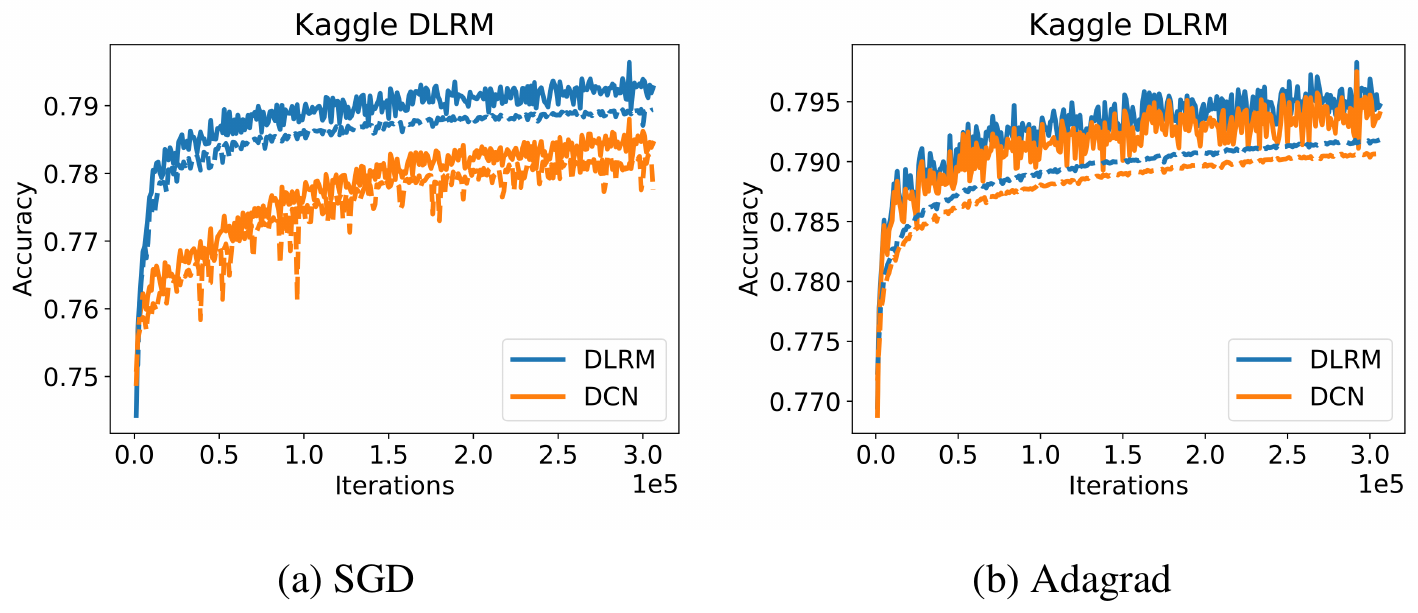
We plot both the training (solid) and validation (dashed) accuracies over a full single epoch of training for both models with SGD and Adagrad optimizers [29]. No regularization is used. In this experiment, DLRM obtains slightly higher training and validation accuracy, as shown in Figure 5. We emphasize that this is without extensive tuning of model hyperparameters.

5.2 Model Performance on a Single Socket/Device

To profile the performance of our model on a single socket device, we consider a sample model with $8$ categorical features and $512$ continuous features. Each categorical feature is processed through an embedding table with $1M$ vectors, with vector dimension $64$, while the continuous features are assembled into a vector of dimension $512$. Let the bottom MLP have two layers, while the top MLP has four layers. We profile this model on a data set with $2048K$ randomly generated samples organized into $1K$ mini-batches[^9].

[^9]: For instance, this configuration can be achieved with the following command line arguments ``--arch-embedding-size=1000000-1000000-1000000-1000000-1000000-1000000-1000000-1000000 --arch-sparse-feature-size=64 --arch-mlp-bot=512-512-64 --arch-mlp-top=1024-1024-1024-1 --data-generation=random --mini-batch-size=2048 --num-batches=1000 --num-indices-per-lookup=100 [--use-gpu] [--enable-profiling]

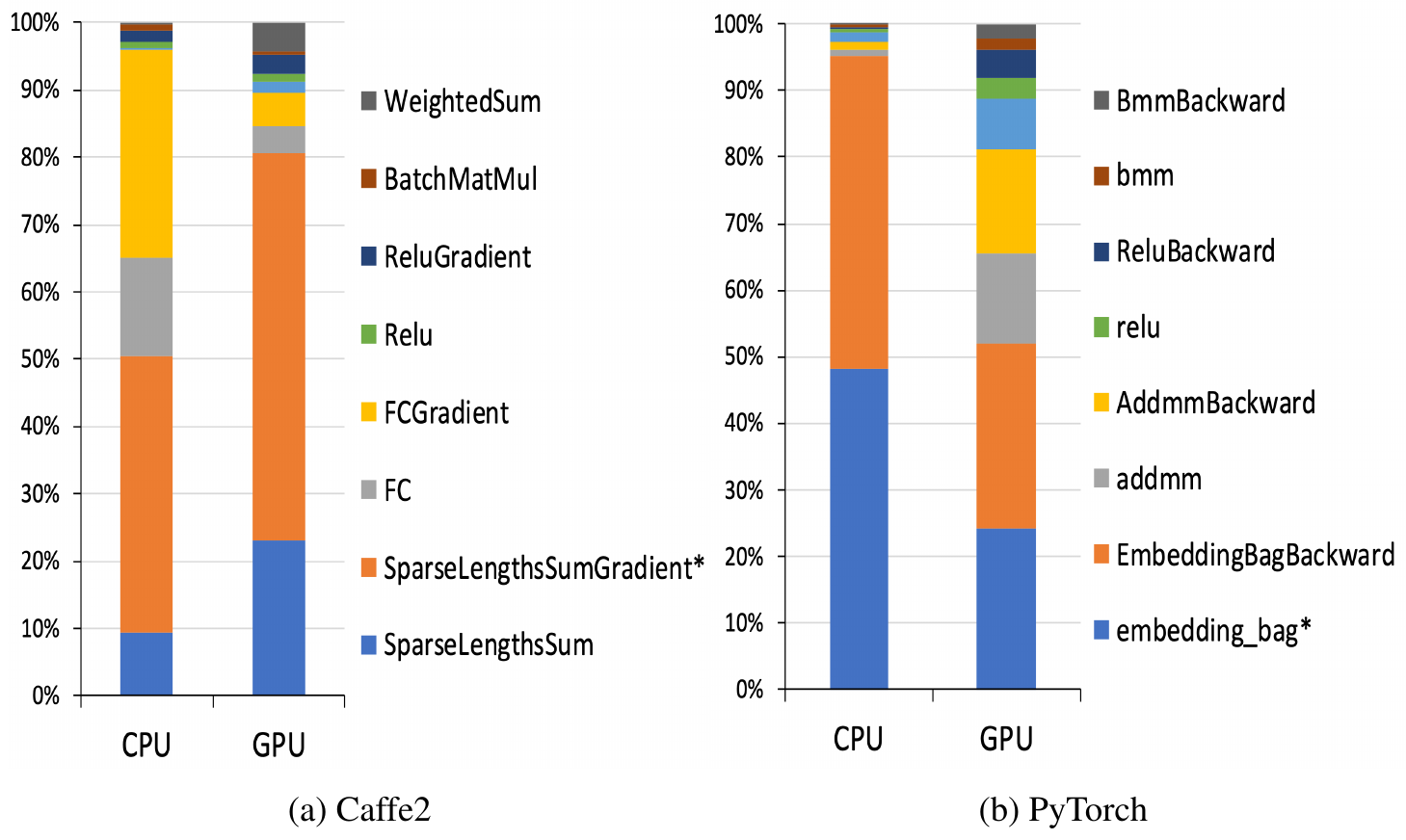
This model implementation in Caffe2 runs in around 256 seconds on the CPU and 62 seconds on the GPU, with profiling of individual operators shown in Figure 6. As expected, the majority of time is spent performing embedding lookups and fully connected layers. On the CPU, fully connected layers take a significant portion of the computation, while on the GPU they are almost negligible.

6. Conclusion

Section Summary: In this paper the authors introduce and publicly release a new deep learning model for recommendation systems that makes use of categorical data. They note that while such systems already drive much of deep learning’s practical success in industry, they remain largely overlooked by academic researchers. By sharing a detailed description of a state-of-the-art example along with its open-source code, the authors aim to highlight the distinctive challenges these models pose and to encourage wider experimentation and study.

In this paper, we have proposed and open-sourced a novel deep learning-based recommendation model that exploits categorical data. Although recommendation and personalization systems still drive much practical success of deep learning within industry today, these networks continue to receive little attention in the academic community. By providing a detailed description of a state-of-the-art recommendation system and its open-source implementation, we hope to draw attention to the unique challenges that this class of networks present in an accessible way for the purpose of further algorithmic experimentation, modeling, system co-design, and benchmarking.

Acknowledgments

The authors would like to acknowledge AI Systems Co-Design, Caffe2, PyTorch and AML team members for their help in reviewing this document.

References

Section Summary: The references section gathers sources that underpin a discussion of recommender systems and related machine-learning methods. It lists foundational texts on matrix factorization, pattern recognition, and statistical models alongside more recent papers on neural networks, deep-learning architectures for click-through-rate prediction, and factorization machines. It also cites software tools, parallel-computing libraries, and privacy techniques such as federated learning and encryption.

[1] Pandora. Music genome project https://www.pandora.com/about/mgp.

[2] Xia Ning, Christian Desrosiers, and George Karypis. A comprehensive survey of neighborhood-based recommendation methods. In Recommender Systems Handbook, 2015.

[3] Evgeny Frolov and Ivan Oseledets. Tensor methods and recommender systems. Wiley Interdisciplinary Reviews: Data Mining and Knowledge Discovery, 7(3):e1201, 2017.

[4] Yehuda Koren, Robert Bell, and Chris Volinsky. Matrix factorization techniques for recommender systems. Computer, (8):30–37, 2009.

[5] Luc Devroye, Laszlo Gyorfi, and Gabor Lugosi. A Probabilistic Theory of Pattern Recognition. New York, Springer-Verlag, 1996.

[6] Strother H. Walker and David B. Duncan. Estimation of the probability of an event as a function of several independent variables. Biometrika, 54:167–178, 1967.

[7] Maxim Naumov. On the dimensionality of embeddings for sparse features and data. In arXiv preprint arXiv:1901.02103, 2019.

[8] Steffen Rendle. Factorization machines. In Proc. 2010 IEEE International Conference on Data Mining, pages 995–1000, 2010.

[9] Gene H. Golub and Charles F. Van Loan. Matrix Computations. The John Hopkins University Press, 3rd edition, 1996.

[10] Corinna Cortes and Vladimir N. Vapnik. Support-vector networks. Machine Learning, 2:273–297, 1995.

[11] Christopher M. Bishop. Neural Networks for Pattern Recognition. The Oxford University Press, 1st edition, 1995.

[12] Xiangnan He, Lizi Liao, Hanwang Zhang, Liqiang Nie, Xia Hu, and Tat-Seng Chua. Neural collaborative filtering. In Proc. 26th Int. Conf. World Wide Web, pages 173–182, 2017.

[13] Suvash Sedhain, Aditya Krishna Menon, Scott Sanner, and Lexing Xie. Autorec: Autoencoders meet collaborative filtering. In Proc. 24th Int. Conf. World Wide Web, pages 111–112, 2015.

[14] MLPerf. https://mlperf.org/.

[15] Adam Paszke, Sam Gross, Soumith Chintala, and Gregory Chanan. PyTorch: Tensors and dynamic neural networks in python with strong GPU acceleration https://pytorch.org/, 2017.

[16] Facebook. Caffe2, https://caffe2.ai, 2016.

[17] Heng-Tze Cheng, Levent Koc, Jeremiah Harmsen, Tal Shaked, Tushar Chandra, Hrishi Aradhye, Glen Anderson, Greg Corrado, Wei Chai, Mustafa Ispir, Rohan Anil, Zakaria Haque, Lichan Hong, Vihan Jain, Xiaobing Liu, and Hemal Shah. Wide & deep learning for recommender systems. In Proc. 1st Workshop on Deep Learning for Recommender Systems, pages 7–10, 2016.

[18] Huifeng Guo, Ruiming Tang, Yunming Ye, Zhenguo Li, and Xiuqiang He. DeepFM: a factorization-machine based neural network for CTR prediction. arXiv preprint arXiv:1703.04247, 2017.

[19] Ruoxi Wang, Bin Fu, Gang Fu, and Mingliang Wang. Deep & cross network for ad click predictions. In Proc. ADKDD, page 12, 2017.

[20] Jianxun Lian, Xiaohuan Zhou, Fuzheng Zhang, Zhongxia Chen, Xing Xie, and Guangzhong Sun. xDeepFM: Combining explicit and implicit feature interactions for recommender systems. In Proc. of the 24th ACM SIGKDD International Conference on Knowledge Discovery & Data Mining, pages 1754–1763. ACM, 2018.

[21] Guorui Zhou, Na Mou, Ying Fan, Qi Pi, Weijie Bian, Chang Zhou, Xiaoqiang Zhu, and Kun Gai. Deep interest evolution network for click-through rate prediction. arXiv preprint arXiv:1809.03672, 2018.

[22] Guorui Zhou, Xiaoqiang Zhu, Chenru Song, Ying Fan, Han Zhu, Xiao Ma, Yanghui Yan, Junqi Jin, Han Li, and Kun Gai. Deep interest network for click-through rate prediction. In Proc. of the 24th ACM SIGKDD International Conference on Knowledge Discovery & Data Mining, pages 1059–1068. ACM, 2018.

[23] Ananth Grama, Vipin Kumar, Anshul Gupta, and George Karypis. Introduction to parallel computing. Pearson Education, 2003.

[24] Sylvain Jeaugey. Nccl 2.0, 2017.

[25] Facebook. Collective communications library with various primitives for multi-machine training (gloo), https://github.com/facebookincubator/gloo.

[26] Keith Bonawitz, Hubert Eichner, Wolfgang Grieskamp, Dzmitry Huba, Alex Ingerman, Vladimir Ivanov, Chloé Kiddon, Jakub Konečný, Stefano Mazzocchi, Brendan McMahan, Timon Van Overveldt, David Petrou, Daniel Ramage, and Jason Roselander. Towards federated learning at scale: System design. In Proc. 2nd Conference on Systems and Machine Learning (SysML), 2019.

[27] Craig Gentry. A fully homomorphic encryption scheme. PhD thesis, Stanford University, 2009.

[28] Rahman Hassan, Antony Harris, Nigel Topham, and Aris Efthymiou. Synthetic trace-driven simulation of cache memory. In Proc. 21st International Conference on Advanced Information Networking and Applications Workshops (AINAW'07), 2007.

[29] John Duchi, Elad Hazan, and Yoram Singer. Adaptive subgradient methods for online learning and stochastic optimization. Journal of Machine Learning Research, 12:2121–2159, 2011.