Learn from your own latents and not from tokens: A sample-complexity theory

Daniel J. Korchinski$^{*}$ Institute of Physics EPFL Lausanne, VD Switzerland [email protected]

Alessandro Favero$^{*}$ Department of Applied Maths and Theoretical Physics University of Cambridge Cambridge, UK [email protected]

Matthieu Wyart Department of Physics & Institute of Physics Johns Hopkins University & EPFL Baltimore, MD USA & Lausanne, VD Switzerland [email protected]

$^{*}$ Equal contribution

Abstract

Generative models, from diffusion models to large language models, achieve remarkable performance but at a cost in training data orders of magnitude larger than what biological learners require. An alternative paradigm has emerged in which networks are trained to predict their own latent representations of related views or masked regions, as in data2vec and JEPA – an idea related to predictive-coding accounts of the cortex. Despite strong empirical results, the theoretical understanding of these methods remains limited. Central questions include: by how much does latent prediction actually improve data efficiency? Is there a benefit to stacking such methods into multi-scale hierarchies? We answer both using as data a tractable probabilistic context-free grammar that captures the compositional structure of natural language and images. Such a grammar generates strings of visible tokens by recursively applying production rules along a tree of hidden symbols of depth $L$. For such data, supervised or token-level SSL require a number of samples exponential in $L$ to recover the latent tree; we prove that latent prediction achieves this with a number of samples constant in $L$, up to logarithmic factors. We confirm this bound with (i) a hierarchical clustering algorithm, (ii) an end-to-end neural network whose predictor-clusterer modules predict their own latents at each level via gradient descent, and (iii) the first sample-complexity analysis of data2vec, which we show implicitly performs hierarchical latent prediction. This suggests that explicit stacking such as H-JEPA is largely redundant.

Executive Summary: Executive Summary

Generative models such as large language models and diffusion models achieve strong performance only after training on orders of magnitude more data than human learners encounter. This inefficiency has prompted interest in alternatives to raw-token prediction, including methods that train networks to predict their own learned latent representations of related or masked inputs (as in data2vec and JEPA). These approaches connect to predictive-coding ideas in neuroscience, yet their quantitative advantages in sample efficiency, and the value of stacking them into explicit multi-scale hierarchies, have remained unclear.

This paper evaluates both questions on synthetic data generated by the Random Hierarchy Model (RHM), a tractable probabilistic context-free grammar with fixed tree depth (L) and branching factor governed by parameter (m). The RHM produces compositional sequences whose latent structure mirrors key properties of language and images. Prior results established that supervised learning and token-level self-supervised objectives require a number of samples that grows exponentially with depth ((\sim vm^{L+1})). The paper asks whether latent-prediction methods can recover the full non-root latent hierarchy with far fewer examples and whether explicit hierarchical stacking adds further benefit.

The analysis combines three complementary approaches. First, an iterative latent-clustering algorithm recovers successive levels by grouping tuples whose empirical context vectors (conditioned on “cousin” tuples at the same scale) coincide. Second, an end-to-end differentiable network consisting of stacked predictor-clusterer modules is trained with gradient descent. Third, the training dynamics of data2vec are analyzed both empirically and theoretically, showing that its student-teacher objective implicitly performs the same per-level clustering.

The central findings are that latent prediction recovers the non-root hierarchy from a number of samples scaling as (vm^3), independent of depth (L) (up to logarithmic factors), whereas token-level objectives remain exponential in (L). This bound is achieved by the clustering algorithm, by the differentiable stacked network, and—surprisingly—by unmodified data2vec. Consequently, a single latent-prediction stage already performs the multi-scale discovery that explicit stacking (as in H-JEPA) was intended to provide; explicit hierarchies therefore appear largely redundant on this data.

These results demonstrate that predicting within the latent space at each level amplifies statistical signal that token-level prediction dilutes, offering a concrete, quantitative explanation for the sample-efficiency gap between current generative models and biological learners. Because the RHM scaling matches empirical observations on real language and images, the same advantage is expected to hold when latent-prediction objectives are applied at scale.

The authors recommend controlled experiments that compare data2vec-style latent prediction against next-token baselines across a wide range of dataset sizes, both alone and in hybrid losses. Architectures that remain effective under strictly local learning rules should also be tested, given their biological plausibility. The principal limitation is that the RHM uses a fixed, unambiguous tree; extensions to variable topologies, recursion, and context-dependent rules are required before the theory can guide architectural choices on natural data.

1. Introduction

Section Summary: The introduction argues that today's diffusion models and large language models succeed only by consuming far more raw data than children need, because they predict tokens rather than higher-level structure. It suggests that self-supervised methods which instead train a network to forecast its own evolving latent representations (as in BYOL, DINO or data2vec) can exploit the hidden hierarchical organization of natural signals and therefore learn much more efficiently. To test this idea the authors introduce a simplified random grammar model whose latent tree depth is known, then show that a latent-prediction scheme recovers the full hierarchy from a number of examples independent of depth—orders of magnitude fewer than are required by ordinary token-level training.

Generative models have reached striking empirical success. Diffusion models produce realistic images and video ([1, 2, 3]), while large language models trained by next-token prediction master grammar, world knowledge and reasoning ([4, 5, 6]). Both rest on a single recipe: predict masked or future fragments of the raw signal at massive scale. Yet this success is bought at a cost biological learners do not pay.

Frontier LLMs are trained on $10^{13}$ – $10^{14}$ tokens ([7, 8]), more than five orders of magnitude beyond what a child encounters before reaching adult-level competence ([9, 10, 11]); state-of-the-art diffusion models likewise rely on billions of images ([12]). This gap suggests that token-level pretraining is far from optimal, and several hypotheses have been advanced to explain it. One is that biological learning is multimodal and grounded ([13, 14]). A second – the one we pursue – is that learning may not be most efficient at the level of raw tokens, but instead in a more abstract latent space ([15, 16, 17]). Indeed, predicting semantic concepts or continuous latents has been shown to improve data efficiency ([18, 19]).

An alternative strategy to input reconstruction has gained traction in the last five years: the network is trained to predict its own latent representations of related views, masked regions or future signals. These targets are themselves the output of a learned encoder, lifting prediction into increasingly abstract spaces as learning progresses. The idea relates to computational neuroscience, where predictive coding posits that the cortex seeks to predict its own future activity ([15, 20, 21]). A growing family of self-supervised methods instantiates this principle, including BYOL ([22]), DINO ([23]), data2vec ([24]) and JEPA ([17]).

Some advantages of these algorithms over input reconstruction approaches have been discussed in the literature, including the fact that they can be formulated as energy-based methods ([17]) or are more robust to the presence of irrelevant features in the data ([25]). Yet understanding why and by how much these methods improve data efficiency remains a fundamental challenge in both machine learning and neuroscience. Another key question is the putative benefits of stacking such algorithms so as to obtain a multi-scale hierarchy of learned representations. This idea, proposed years ago ([17]), was recently implemented ([26, 27]) and appears to lead at best to moderate improvements, for reasons that remain currently unclear.

In this work, we address both questions by focusing on synthetic models of data with a hierarchical latent structure. Probabilistic context-free grammars (PCFGs) are a natural candidate: through recursive production rules they generate data compositionally from a tree of latent variables, and have long been influential as models of language ([28, 29]) and natural images ([30, 31]). General PCFGs are notoriously hard to treat. We therefore work with the Random Hierarchy Model (RHM) ([32]), a simplified PCFG with fixed tree topology and random production rules. The RHM has produced quantitatively predictive theories, including relating neural scaling laws to the statistics of natural language ([33, 34]), and a theory of compositional generalization and memorization in diffusion models for language and images ([35, 36, 37]). The RHM is parameterized by the number of production rules per symbol, $m$, and the depth of the latent tree, $L$. Prior work shows that for deep architectures, supervised end-to-end learning requires an order of $m^L$ samples ([32]), and token-level self-supervised objectives – masked-language modelling and diffusion – require of order $m^{L+1}$ ([33, 38, 39]). Both costs grow exponentially with the depth $L$ of the latent hierarchy (and thus polynomially in the input dimension, i.e., sequence length). Against this baseline, we establish three results:

Efficient algorithm for representation learning (Section 3). We show that a hierarchical clustering algorithm recovers the full non-root latent tree from order $m^3$ samples – independent of the depth $L$, and hence exponentially fewer than those required by token-level SSL.
An end-to-end stacked architecture with the same scaling (Section 4). We propose a new architecture where a stack of small predictor-clusterer modules predicts its own latents at each level. Trained end-to-end with gradient descent, it reaches the $m^3$ scaling on the RHM.
A theory of data2vec (Section 5). We show empirically and explain theoretically with reasonable assumptions that data2vec ([24]) implicitly performs hierarchical latent prediction, again leading to a sample complexity of order $m^3$. To our knowledge, this is the first sample-complexity analysis of such methods.

These results establish that learning from one's own latents can yield huge sample-complexity gains over token-level objectives. They also show that a single latent-prediction module such as data2vec is in effect already performing multi-scale latent discovery. Such methods may already be implicitly hierarchical, weakening the case for explicit stacking such as H-JEPA.

Related work.

The compositional and hierarchical structure of natural data has long been put forward as a key feature making it learnable by neural networks. Deep networks represent hierarchically compositional functions with exponentially fewer parameters than shallow ones ([40]), yielding nonparametric sample-complexity bounds polynomial in the input dimension for both supervised ([41]) and self-supervised ([42]) tasks. These results characterize expressivity and information-theoretic statistics, but do not describe what gradient descent can actually learn from finite data. A complementary line shows that transformers can approximately implement parsing-style inference on context-free grammars ([43, 44, 45]), characterizing the algorithm trained models implement, but not its sample complexity. The RHM ([32]), building on [46], [47], and [48], fills this gap by enabling sample-complexity predictions that match observations in deep nets. Existing RHM analyses cover supervised learning ([32]) and token-level SSL ([33, 38]), but not learning from one's own latents, which is the focus of this work.

2. Preliminaries

Section Summary: The Random Hierarchy Model generates data from a fixed-depth tree of production rules, where each level maps groups of synonymous child tuples to a latent parent symbol according to an unknown grammar. Learning the model requires identifying these synonym classes by detecting correlations between a tuple and some observable variable elsewhere in the tree; each unresolved rule along the path attenuates the signal and multiplies the needed sample size by roughly the branching factor m. Supervised classification and token-level self-supervised objectives therefore face steep sample-complexity costs set by the weakest long-range correlations, whereas directly supervising on latent variables avoids the worst bottlenecks.

$**Figure 1:** **The sample complexity $P$ to learn RHM data depends on training objective**. The sample complexity to learn the synonymic invariance of correlations (and construct latent $\star$) between prediction target ($Z$, boxed) and its context tuple ($T$, circled) scales as $m^{d_{tree}}$, where $d_{tree}$ denotes the tree-distance between the two. Overall sample complexity is bottlenecked by the weakest pertinent correlations, which we highlight for supervised classification and token-level SSL. Supervising on latents, as our ILC algorithm (Section 3), SLC network (Section 4), and data2vec (Section 5) do, achieves the better sample complexity $\sim m^3$.$

The Random Hierarchy Model (RHM).

The RHM ([32]) is a probabilistic context-free grammar on a fixed regular tree. The tree has depth $L$, branching factor $s$, and vocabularies $\mathcal V_0, \mathcal V_1, \ldots, \mathcal V_L$, all of size $v$ . Level $0$ is visible and levels $1, \ldots, L$ are latent. At level $\ell$, there are $s^{L-\ell}$ variables $h^{(\ell)}1, \ldots, h^{(\ell)}{s^{L-\ell}}$, with $h^{(\ell)}u\in\mathcal V\ell$ . The visible sequence is $x_i=h^{(0)}_i$, $i=1, \ldots, s^L$ .

For each level $\ell=0, \ldots, L-1$, a grammar instance is sampled by choosing $vm$ distinct tuples from $\mathcal V_\ell^s$ uniformly without replacement and partitioning them into $v$ labeled groups of size $m$, one group $\mathcal R_{\ell, a}$ for each parent symbol $a\in\mathcal V_{\ell+1}$ . A rule $\nu=(\nu_1, \ldots, \nu_s)\in\mathcal R_{\ell, a}$ means that parent $a$ may generate the tuple of children $\nu$ . The set of grammatical tuples at level $\ell$ is $\mathcal S_\ell:=\bigsqcup_{a\in\mathcal V_{\ell+1}}\mathcal R_{\ell, a}, $ so $|\mathcal S_\ell|=vm$ . We write $f:=m/v^{s-1}$ for the fraction of valid $s$ -tuples, since $vm$ out of the $v^s$ possible tuples are grammatical. Because the rule map is injective, the grammar is unambiguous: each grammatical tuple has a unique parent. We denote it by $\mathrm{par}\ell(\nu)=a ;\Longleftrightarrow; \nu\in\mathcal R{\ell, a}.$ Two grammatical tuples $\nu, \nu'\in\mathcal S_\ell$ are called synonyms if they have the same parent.

Generation proceeds top-down. First $h^{(L)}1\sim\mathrm{Unif}(\mathcal V_L)$ . Then, recursively, if $h^{(\ell+1)}u=a$, the child tuple $T^{(\ell)}u:=\big(h^{(\ell)}{(u-1)s+1}, \ldots, h^{(\ell)}{us}\big)$ is sampled uniformly from $\mathcal R{\ell, a}$ .

Correlation-based learning in the RHM.

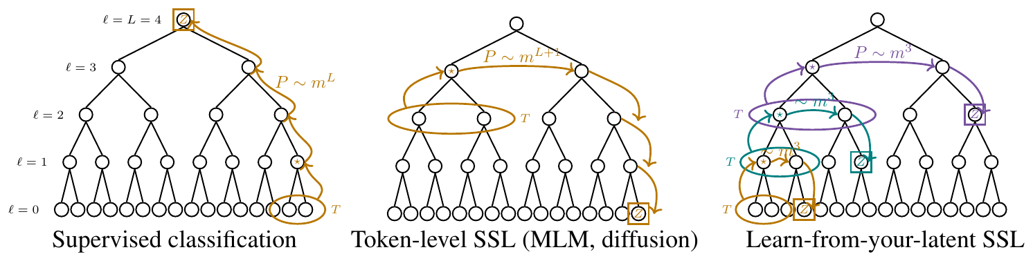
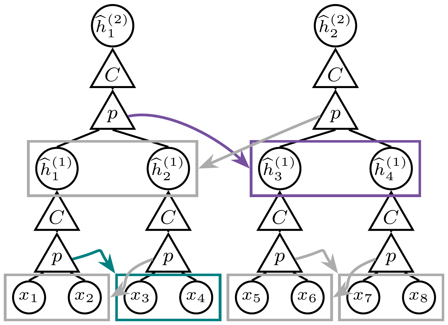
A central observation from [32] is that learning the RHM amounts to learning invariances under the exchange of synonyms. The statistical signal that identifies these synonym classes comes from correlations between a tuple and an external observable. Concretely, let $T^{(\ell)}$ be a level- $\ell$ tuple and let $Z$ be an observable elsewhere in the tree. This arrangement is depicted for different learning objectives in Figure 1. One can consider the connected correlation:

$ C_Z(\nu, z) := \mathbb P[T^{(\ell)}=\nu, Z=z]

\mathbb P[T^{(\ell)}=\nu]\mathbb P[Z=z]. $

If two tuples $\nu, \nu'$ are synonyms, then $C_Z(\nu, \cdot)=C_Z(\nu', \cdot), $ whenever $Z$ depends on the tuple only through its parent.[^1] The strength of this correlation signal depends on the choice of $Z$ and on its position relative to the tuple. The signal must propagate through the hidden tree from the parent of $T^{(\ell)}$ to the observable $Z$ . Along this path, each unresolved production rule averages over $m$ synonymous choices, attenuating the signal. In sample-complexity terms, each additional unresolved rule costs a factor of order $m$, as illustrated in Figure 1.

[^1]: Indeed, conditioned on the parent of the tuple, the rest of the tree is independent of which production rule was used to generate the tuple, and the uniform choice of production rules gives $\mathbb P[T^{(\ell)}=\nu]=\mathbb P[T^{(\ell)}=\nu']$ within each synonym class.

Supervised classification ([32]): the observable $Z$ is the class label at the root. To recover the rules mapping level- $\ell$ tuples to level- $(\ell+1)$ latents, the root-to-tuple correlation must traverse the $L-\ell-1$ levels separating the tuple parent from the root. Including the fact that each grammatical tuple is observed with probability of order $1/(vm)$, this gives sample complexities of the form $P_\ell^{sup} \asymp v, m^{L-\ell}.$ The hardest step is therefore the first one, $\ell=0$, where one must learn the level-1 rules. Deep networks trained on the supervised RHM classification task were found to saturate this scaling and reconstruct the latent hierarchy in their representations.

Token-level self-supervision ([33, 38, 39]): $Z$ is a masked or noised token. In the first step, local correlations between visible tokens identify the level-1 synonym classes, with sample complexity $P_1^{tok} \asymp v m^3.$ Once these low-level latents have been internally reconstructed, the model can use them as coarse context variables. To learn higher levels, the relevant statistics are token–latent correlations: a visible token is correlated with a latent representation of its context. However, because the prediction target is still a surface token, the signal is averaged through the descendant channel from the latent scale down to the leaves. Each additional latent level therefore costs one extra factor of $m$ in sample complexity. Thus, if $\ell \geq 1$ denotes the latent level being learned above the leaves,

$ P_\ell^{\mathrm{tok}} \asymp v, m^{\ell+2}.\tag{1} $

Neural networks trained with token-level SSL objectives were empirically shown to saturate this staged scaling: as the dataset size increases, lower-level latents appear first, and higher-level latents become learnable thereafter. The overall sample-complexity is gated behind reconstructing latents $\ell = L-1$ leading to $P_{tok}\asymp vm^{L+1}$.[^2]

[^2]: Notice that since the root is sampled uniformly and each root symbol has $m$ equiprobable rules, the distribution does not reveal how the $vm$ valid top-level tuples are partitioned into $v$ groups of size $m$, one group per root symbol. Thus unsupervised learning can recover $h^{(1)}, h^{(2)}, \ldots, h^{(L-1)}$ and the support of valid top-level tuples, but not the root labels themselves.

3. Recovering the RHM hierarchy by clustering

Section Summary: The section explains how to recover an entire latent hierarchy by iteratively clustering observed tuples according to their empirical context vectors, which serve as reliable signatures of their hidden parent variables. Once one level has been decoded, the same local clustering task can be repeated at the next level with no increase in difficulty or sample requirement, so the full non-root hierarchy is obtained from roughly the same number of examples (order vm^3) needed to learn the first level. A simple iterative algorithm based on this idea is shown both theoretically and numerically to succeed with high probability under mild statistical assumptions on the grammar.

**Algorithm 1:** Iterative Latent Clustering (ILC) — see Figure 2 for a graphical representation.

As discussed in the previous section, the limitation of token-level objectives is not that they fail to learn latent variables. Rather, they learn them while still receiving supervision through visible tokens. The learn-from-your-own-latent setting studied below removes this residual token bottleneck: once level $\ell$ has been recovered, both the conditioning object and the prediction target are lifted to level $\ell$ . The next stage is then again a local synonym-clustering problem, but now with the same statistical strength at every scale.

In other words, every level becomes as easy as the first token-level step. Given Equation 1, this suggests that the whole non-root hierarchy should be recoverable from $P\asymp vm^3$ samples. This is illustrated in Figure 1–right.

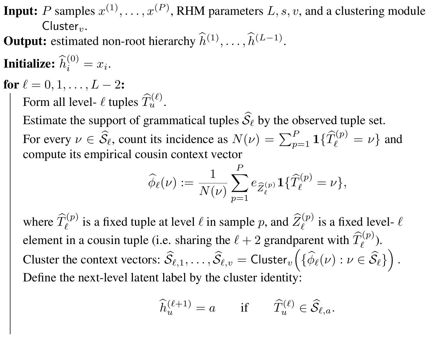
Iterative latent-clustering algorithm (ILC).

The preceding section framed learning the RHM in terms of learning tuple-target correlations, and identifying synonyms by tuples that share identical correlations. Here, we cast this as a vector-clustering problem. Let $T$ denote a level- $\ell$ tuple, let $Z$ be a level- $\ell$ target in a cousin tuple (cf. the arrangement in Figure 1 – cousins are simply nodes sharing the same grandparent at level $\ell+2$), and let $e_Z\in\mathbb R^v$ be its one-hot encoding. For each grammatical tuple $\nu\in\mathcal S_\ell$, define the conditional context vector

$ \phi_\ell(\nu) := \mathbb E[e_Z\mid T=\nu] \in\Delta^{v-1}. $

**Figure 2:** **Graphical representation of Algorithm 1 for $L=3$**. Predictor $p$ implements steps 3-5, and clusterer $C$ constructs next-level latents. Highlighted prediction targets are as in Figure 1–**right**.

As before, the essential observation is that synonyms have the same context vector. If $\nu\in\mathcal S_{\ell, a}$, we denote the common context vector of parent $a$ by $\Phi_{\ell, a} := \phi_\ell(\nu)$ . The goal is to cluster the $vm$ tuple context vectors into these $v$ parent centers. This assignment of tuples into clusters explicitly constructs the next-level latents.

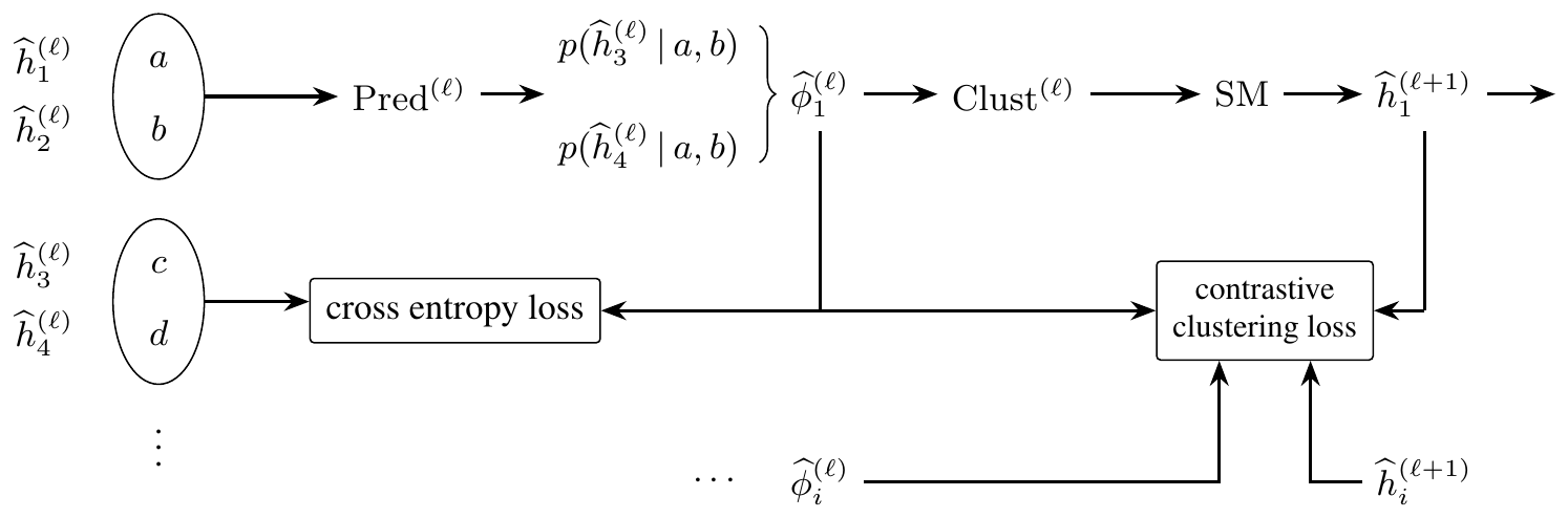
Algorithm 1 (Iterative Latent Clustering, or ILC) operationalizes this procedure. At each step, the algorithm assumes that level $\ell$ has been decoded, clusters level- $\ell$ tuples by their empirical context vectors, and thereby constructs level $\ell+1$ . This clustering procedure is illustrated graphically in Figure 2: the predictor $p$ estimates context vectors (steps 3-5), while the clusterer $C$ maps these vectors to next-level latent labels (steps 6-7). We prove its sample complexity in Theorem 1 and validate it numerically in Figure 3.

Theoretical sample complexity.

An RHM grammar is balanced if, for every level $\ell$, every grammatical tuple occurs with probability of order $1/(vm)$. It is separated if every pair of parent context vector $ \Phi_{\ell, a}, \Phi_{\ell, b} $ are separated by distance $ \gtrsim 1/m$ . We refer the reader to Appendix B for the formal statements of these assumptions and their justification in the limit of $v\to\infty$ at fixed $f \in(0, 1)$. For a balanced and separated RHM grammar with $f<1$, and assuming the existence of a stable clustering module (see Appendix B), we have:

########## {caption="Theorem 1: Recovery of the non-root hierarchy; informal"}

Fix an RHM grammar that is balanced and separated, and a clustering algorithm stable under perturbations. Then there exists a constant $C>0$, depending only on the constants in those assumptions and on $s$, such that the following holds. If

$ P \geq C \left[vm\log\frac{Lvm}{\delta} + \frac{v m^3}{1-f} \log\frac{Lvm}{\delta} \right],\tag{2} $

then the iterative latent-clustering algorithm recovers $h^{(1)}, h^{(2)}, \ldots, h^{(L-1)}$ and all production-rule classes below the root with probability at least $1-\delta$, up to independent permutations of the latent labels at each level.

In particular, for fixed $f$ bounded away from $1$ and up to logarithmic factors, $P_{ILC} \asymp v m^3.$

In Appendix B, we give the formal theorem and its proof, which is a level-by-level induction based on concentration of the empirical context vectors. Notice that $v m^3$ is the scale needed to learn the first-level rules from visible tokens (see Section 2). However, once one level has been recovered, the decoded latent sequence is again an RHM with the same local parameters. The same sample scale therefore suffices at every subsequent level, allowing the algorithm to recover the non-root hierarchy without any exponential dependence on $L$, as illustrated in Figure 1–right.

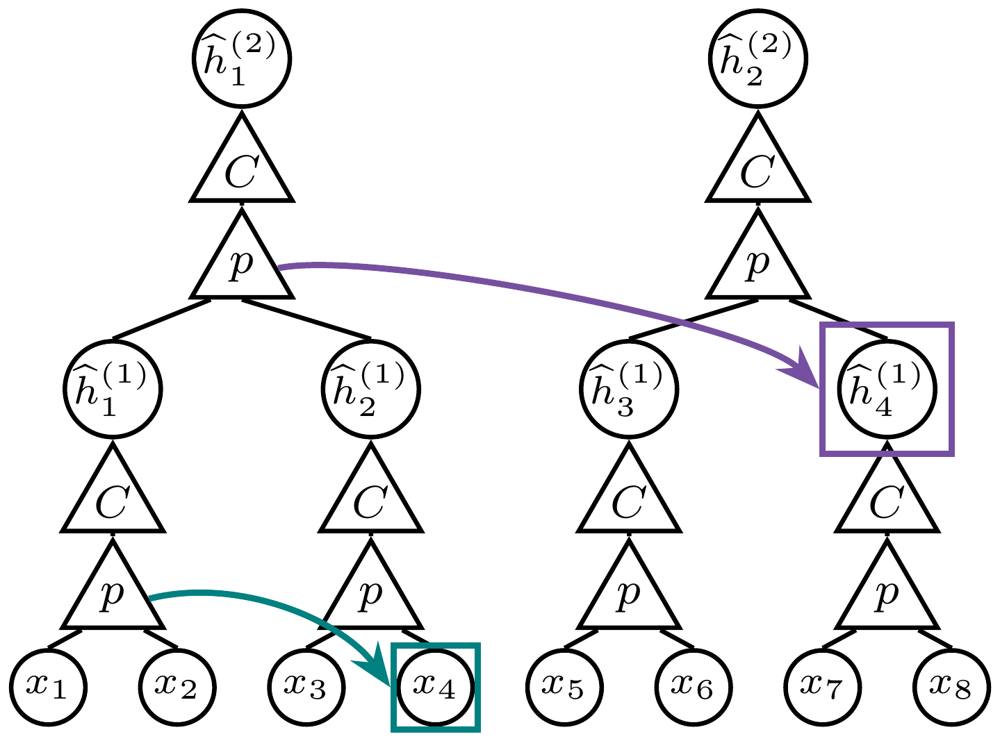
Numerical validation.

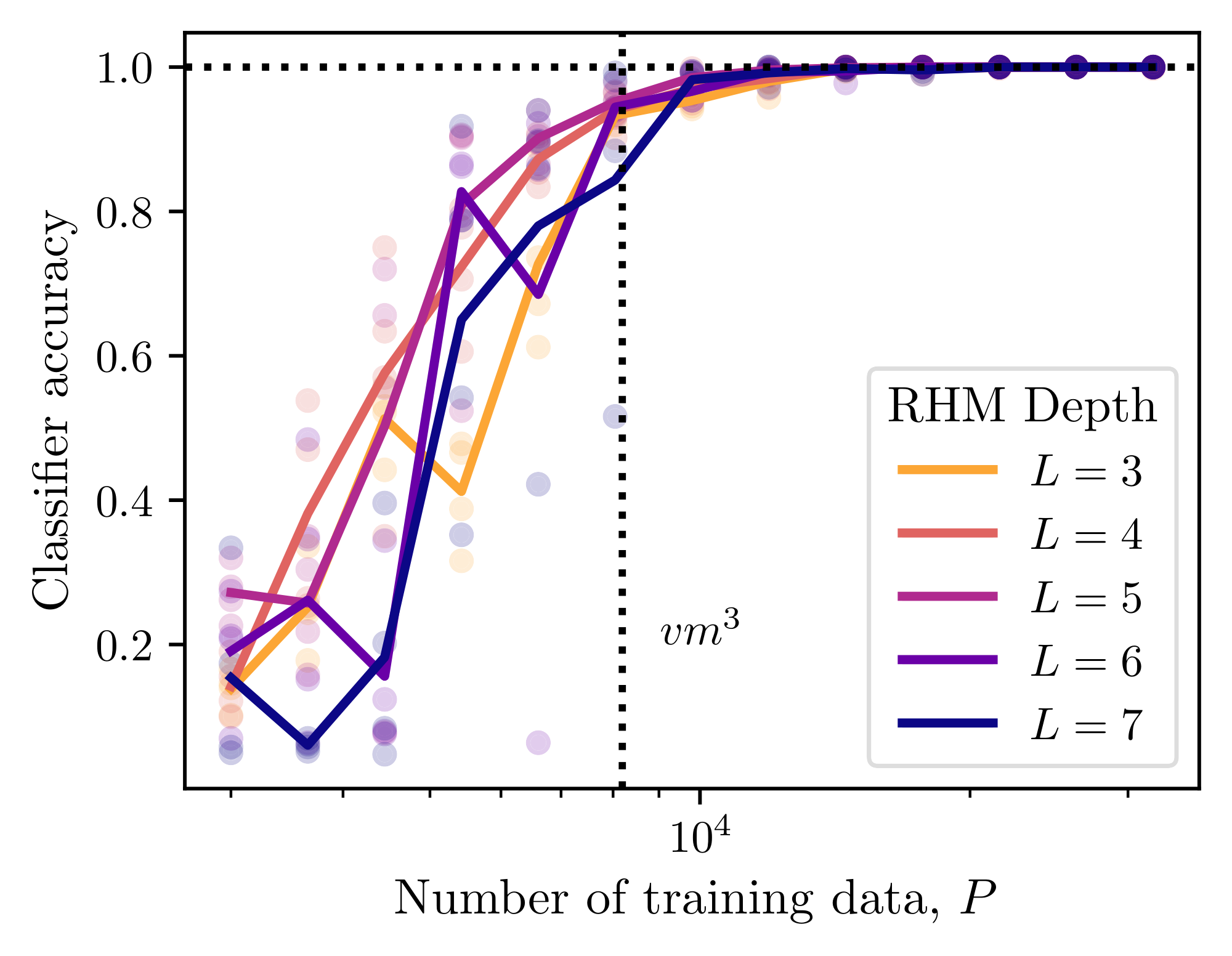
We generate samples from the fixed-tree RHM and apply the level-by-level procedure described above. At each level, we estimate the empirical context vectors $\widehat{\phi}_\ell(\nu)$ for observed grammatical tuples and cluster them using $k$ -means. The recovered labels are matched to the ground-truth latent labels by the optimal permutation, and we report the resulting reconstruction accuracy. Figure 3–left shows the reconstruction accuracy for $L=5$, $s=3$, $v=8$, and varying $m$ . In the unrescaled plot, the transition to perfect reconstruction shifts to larger sample sizes as $m$ increases. After rescaling the number of samples by $v m^3, $ the curves collapse and reconstruction becomes accurate once $P/ v m^3$ is of order one. This confirms the predicted $m^3$ scaling of the local clustering threshold. The algorithm recovers all non-root levels at this same scale, consistent with the theory that the first-level recovery threshold is sufficient to climb the hierarchy recursively.

$**Figure 3:** **Recursive clustering recovers the RHM hierarchy at the predicted scale.** **Left**: Clustering reconstruction accuracy of the iterative clustering algorithm using $k$ -means ($L=5, s=3, v=8$). **Right**: Class reconstruction accuracy of stacked SLC architecture ($L=4, s=3, v=10$) trained end-to-end, evaluated by linear probe on the highest level latents $\widehat{h}^{(L-1)}$. In each panel, the main plot is a *scaling collapse*, effected by rescaling number of samples by predicted sample complexity $P\sim vm^3$. Insets show raw data (top left) and inferred sample complexity (bottom right) $P^\ast$ for which accuracy reaches 50%.$

4. Gradient-based Iterative Latent Clustering

Section Summary: The section investigates whether a neural network trained end-to-end via gradient descent can match the efficient scaling of the iterative latent clustering algorithm. The authors introduce the stacked latent-clustering network, built from repeated modules that each use a predictor to forecast related tokens and a clusterer to assign representations to discrete codes through contrastive objectives, stabilized by an exponential-moving-average teacher network. Experiments show this architecture recovers the theoretical sample-complexity bound even with local learning rules, establishing that explicit hierarchical designs can extract multi-level latent structure.

In this section, we ask whether the same scaling of the ILC algorithm can be achieved by a differentiable architecture trained end-to-end by gradient descent.

The Stacked Latent-Clustering (SLC) network.

We mirror the recursion of Algorithm 1 with a stack of $L-1$ identical modules (Figure 2). Each module is composed of two subnetworks that play the roles of the two operations in the algorithm.

$p$: A predictor $\mathrm{Pred}^{(\ell)}$ takes an $s$-tuple of level- $\ell$ tokens and outputs, via cross-entropy training, a categorical distribution over its cousin tokens; this is the neural analog of the empirical cousin context vector.
$C$: A clusterer $\mathrm{Clust}^{(\ell)}$ then maps each prediction vector to a soft assignment in a discrete codebook through a contrastive objective: prediction vectors with high similarity are pulled to the same code while dissimilar ones are pushed apart – implementing $\mathsf{Cluster}_v$ in the neural setting.

The cluster assignments $\widehat{h}^{(\ell+1)}$ produced by level $\ell$ become the input tokens of the level- $(\ell+1)$ module. To keep the difficulty of the prediction task constant across depth, cluster outputs are tokenized with a softmax. Prediction targets are computed by a teacher network whose weights track an exponential moving average of the student, $W_teacher \leftarrow (1-\alpha_ema), W_teacher + \alpha_ema, W_student, $ a common trick to prevent the representation collapse common to self-distilled SSL [49]. Full architectural and training details are given in Appendix C.1.

Results.

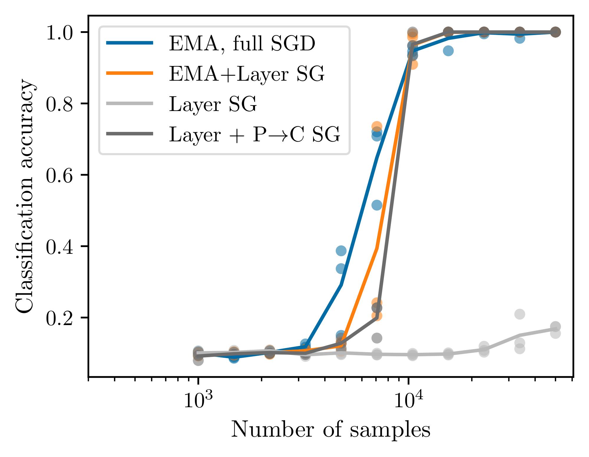
Figure 3–right shows the accuracy of a linear probe trained to recover the top-level latent from the frozen final-layer representations of an SLC network, for $L=4$, $s=3$, $v=10$, and varying $m$. Rescaling the sample axis by $vm^3$ collapses the curves, confirming that the network saturates the clustering threshold of Theorem 1. Figure 12 shows that the sample complexity for $L\in {3, \ldots, 7 }$ does not vary. Interestingly, inserting a stop-gradient at every module boundary (or even between $p$ and $C$), so that each level is trained only by its own prediction and clustering losses, leaves the $vm^3$ scaling unchanged (Figure 9). SLC therefore admits a strictly local learning rule, consistent with biologically motivated learning schemes.

SLC shows that an explicit hierarchical architecture, with one predictor-clusterer module per latent level, can saturate the $vm^3$ statistical bound of Section 3. In the next section, we demonstrate that the SSL representation learning objective of data2vec leads to implicit hierarchical supervision, and correspondingly also saturates this learning bound.

5. Analysis of data2vec

Section Summary: The section argues that data2vec implicitly performs the same iterative latent clustering seen in SLC by using a slowly updated teacher network whose averaged hidden representations serve as soft targets for a student that processes masked inputs. Experiments on the random hierarchy model show that this yields a sample complexity of order vm³ to recover the full non-root hierarchy—far better than token-level prediction would allow and even better than fully supervised learning. The authors explain the scaling through two assumptions on how targets encode previously learned latents and how gradient descent extracts detectable correlations, leading to a phased progression in which each update of the teacher lifts the problem to the next level of the hierarchy.

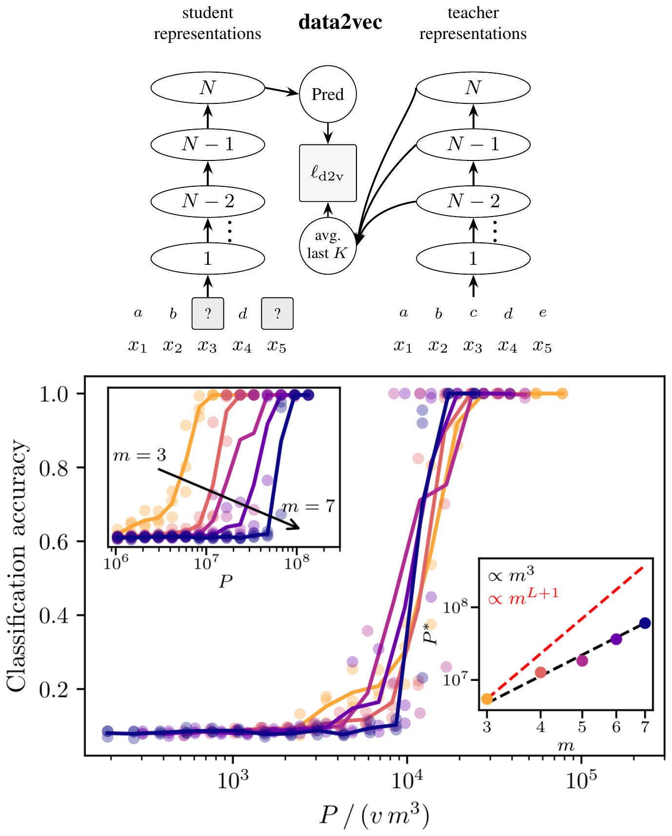
$**Figure 4:** **Data2vec on RHM.** **Left:** data2vec learns in a teacher-student setting; the student is supervised on reconstruction of pooled teacher representations at masked token positions. **Right:** Root-classification accuracy of probes on pooled final-layer features, as a function of the number of online pretraining samples $P$. RHM parameters: $v=16$, $s=2$, $L=4$. Inset: raw curves vs. $P$ and inferred sample complexity $P^\ast$ for which accuracy reaches 50%. Main: rescaling by $vm^3$, curves collapse. Lines are averages over three independent realizations, dots are individual runs.$

In this section, we argue that the iterative clustering mechanism is implicit in data2vec [24], a popular SSL method that predicts its own latent representations. We choose data2vec over the closely related JEPA family because it comes with a published recipe for discrete-token inputs. In particular, data2vec uses a student-teacher setup. The student network is fed a partially masked input $S$; the teacher sees the unmasked input $x$. At every masked position $i$, the student is trained, with a squared loss, to predict the target $Y_i(x)$ given by the average of the last $K$ block activations of a teacher network applied to the unmasked input $x$, as illustrated in Figure 4–left. As with SLC, the teacher has the same architecture as the student, and its weights track an exponential moving average of the student's weights, updated after each gradient step.

Empirical sample complexity.

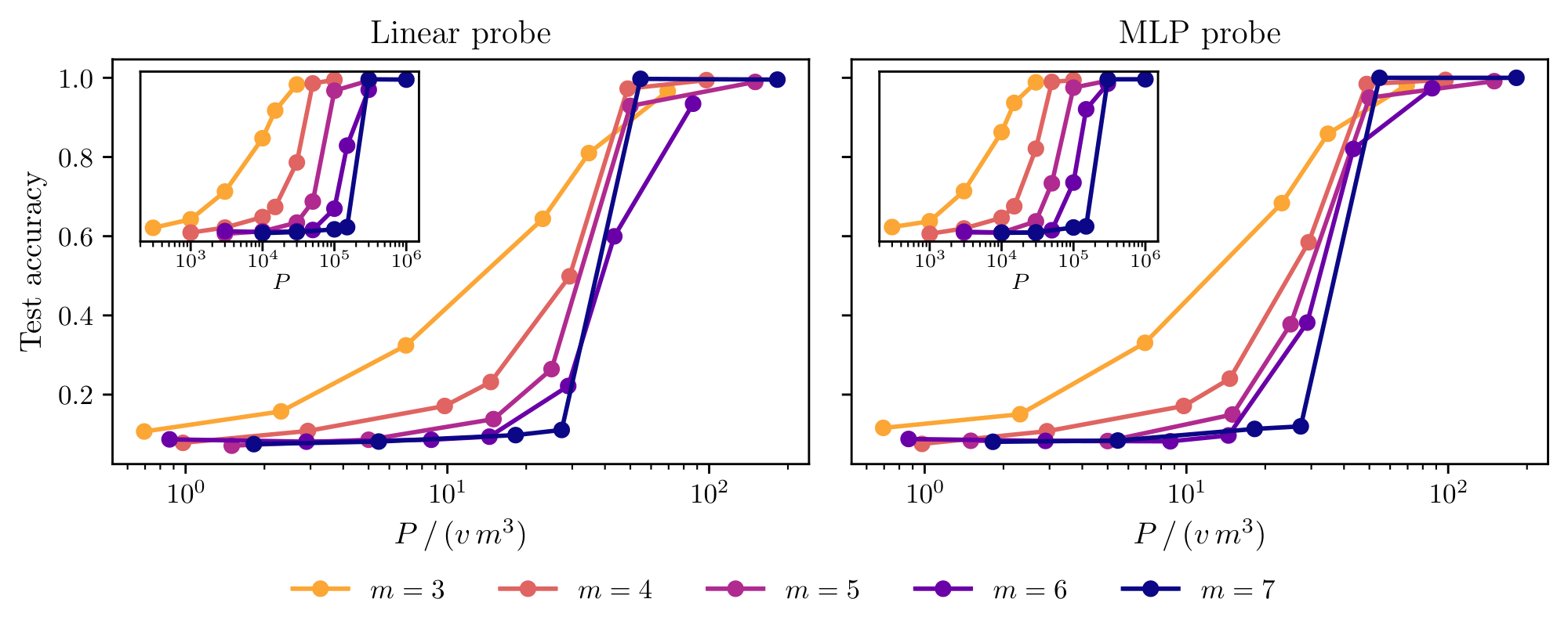
We pretrain data2vec on the RHM. We follow the data2vec text recipe: a fraction $p_{mask}=0.15$ of positions are masked. Full details are presented in Appendix D. We compare two data-presentation regimes: online, where each step draws a fresh batch from the grammar, and offline, where a fixed training set of $P$ unique strings is reused across epochs. After pretraining, we freeze the encoder and train a one-hidden-layer MLP probe to predict the root label from mean-pooled final-layer features.

Figure 4–right shows the downstream root-classification accuracy of the probes for $L=4$, $s=2$, $v=16$ in the online setting.[^3] The learning curves collapse onto a single curve after rescaling the sample axis by $vm^3$. Root classification on the RHM requires resolving all $L-1$ non-root latent levels and then identifying the partition of top-level tuples into root classes. As discussed in Section 2, token-level SSL is bottlenecked by learning the level- $(L-1)$ rules from tokens, which costs $\sim vm^{L+1}=vm^5$ samples; an additional $\mathcal O(vm)$ labeled examples then suffice to learn the root partition.[^4] The observed scaling is hence incompatible with this token-level prediction baseline.

[^3]: The same plots are reported in Appendix D for the offline setting.

[^4]: For reference, fully supervised learning of the root from leaves would itself require $\sim vm^L=vm^4$ samples, so the $vm^3$ scaling we observe is in fact better than what supervised learning achieves – and data2vec uses no labels during pretraining.

Theoretical analysis.

We now explain the $vm^3$ scaling by tying data2vec back to the iterative latent clustering mechanism of Section 3. Although the target $Y_i(x)$ is a continuous vector, we posit it acts as a soft encoding of the RHM latents that the encoder has already learned: at any point in training, $Y_i(x)$ contains a linear component of every latent learned in the encoder (as we verify in Figure 13). We idealize the slow EMA as a discretized sequence of phases: within each phase, the teacher is held fixed, and between phases it is refreshed to absorb the latents most recently acquired by the student. The argument then proceeds by induction over the levels. Phase $0$ reduces data2vec training to the token-level masked-prediction problem of Section 2 and recovers the level- $1$ latents at $P\gtrsim vm^3$. Each subsequent phase lifts the prediction problem onto level- $\ell$ tuples, where it coincides with the cousin-tuple clustering problem of Section 3 – with the same sample complexity. The full non-root hierarchy is therefore recovered at this scale. We now formalize this argument through two assumptions.

(A1) Targets carry the learned latents. Let $z_i^{(\ell)}:=h^{(\ell)}_{\lceil i/s^\ell\rceil}$ be the level- $\ell$ ancestor of position $i$, and let $e_z\in\mathbb R^v$ denote the one-hot encoding of a latent symbol $z$. If the encoder linearly represents the latents $h^{(1)}, \ldots, h^{(\ell)}$, then the teacher target admits a decomposition

$ Y_i(x) ;=; F_i(S) ;+; \sum_{a=0}^{\ell} B_a, e_{z_i^{(a)}} ;+; residual, $

where $F_i(S)$ collects components determined by the visible input and the matrices $B_a$ are non-zero linear projections. The residual term collects everything else, which is typically nonlinear and not used in our analysis. The residual architecture of the transformer makes this natural: a feature decodable from one block propagates through the identity path to every later block, and hence appears with a non-zero linear coefficient in the layers entering the top- $K$ teacher average. At initialization, $\ell=0$ and the only ancestor is $x_i$ itself, so $Y_i(x)$ contains a linear component of the masked one-hot inputs.

(A2) Correlation learning. Whenever a correlation between the prediction target and a feature of the visible input becomes detectable above sampling noise, gradient descent extracts that feature. This is the same correlation-learning hypothesis used in previous RHM analyses [33, 38], where it is supported empirically and by one-step gradient calculations.

Phase 0.

The population minimizer of the data2vec loss is the conditional expectation $\mathbb E[Y_i(x)\mid S]$. By linearity of conditional expectation, in phase $0$, predicting $Y_i(x)$ from $S$ reduces, up to the visible component and the non-linear residual, to predicting the masked one-hot $e_{x_i}$ from its visible context. This is exactly the token-level masked-prediction problem analyzed in Section 2: local token–token correlations become detectable above $P\gtrsim vm^3$, and by (A2) the network extracts them. The resulting representation collapses synonymous level- $0$ tuples onto a common image, and the level- $1$ ancestor becomes linearly decodable from the encoder.

Phase $\ell\geq 1$.

Suppose phases $0, \ldots, \ell-1$ have produced linearly decodable representations of $h^{(1)}, \ldots, h^{(\ell)}$ inside the encoder. After the next teacher update, these latents enter the target, and (A1) gives the new component $\mathbb E[e_{z_i^{(\ell)}}\mid S]$ in the optimal predictor. Because levels $1, \ldots, \ell$ are decodable, the visible context $S$ can be parsed into level- $\ell$ symbols away from the masked position. In particular, it contains the level- $\ell$ cousin tuple $T_\ell$, the closest level- $\ell$ tuple sitting outside the production rule of position $i$. Conditioning on $T_\ell$ produces the context vector $\phi_\ell(\nu)=\mathbb{E}[e_{z_i^{(\ell)}}\mid T_\ell=\nu]$ studied in Section 3. The prediction problem at scale $\ell$ has lifted from leaves to level- $\ell$ tuples, and is now identical to the clustering problem solved by the ILC algorithm of that section, requiring $P\gtrsim vm^3$. When the network extracts this signal, the level- $(\ell+1)$ ancestor $z_i^{(\ell+1)}$ becomes linearly decodable, and the next teacher update carries it into the target.

The induction continues up to $\ell=L-2$. Every phase shares the same sample complexity. Since the same training set is reused across phases, the offline sample complexity equals the per-phase threshold, $P_{d2v} ;\asymp; vm^3$, and depth enters only through the number of phases, not through the per-phase requirement.

$**Figure 5:** **Data2vec clusters synonyms.** Synonym clustering score $\mathcal C_\ell$ of the encoder at $\ell\in\{1, 2, 3\}$, for $L=4$, $s=2$, $v=16$. A positive score means synonyms are mapped closer together than non-synonyms. *Insets:* raw curves vs. $P$. *Main:* same curves rescaled by $vm^3$ collapse.$

The encoder internally clusters synonyms.

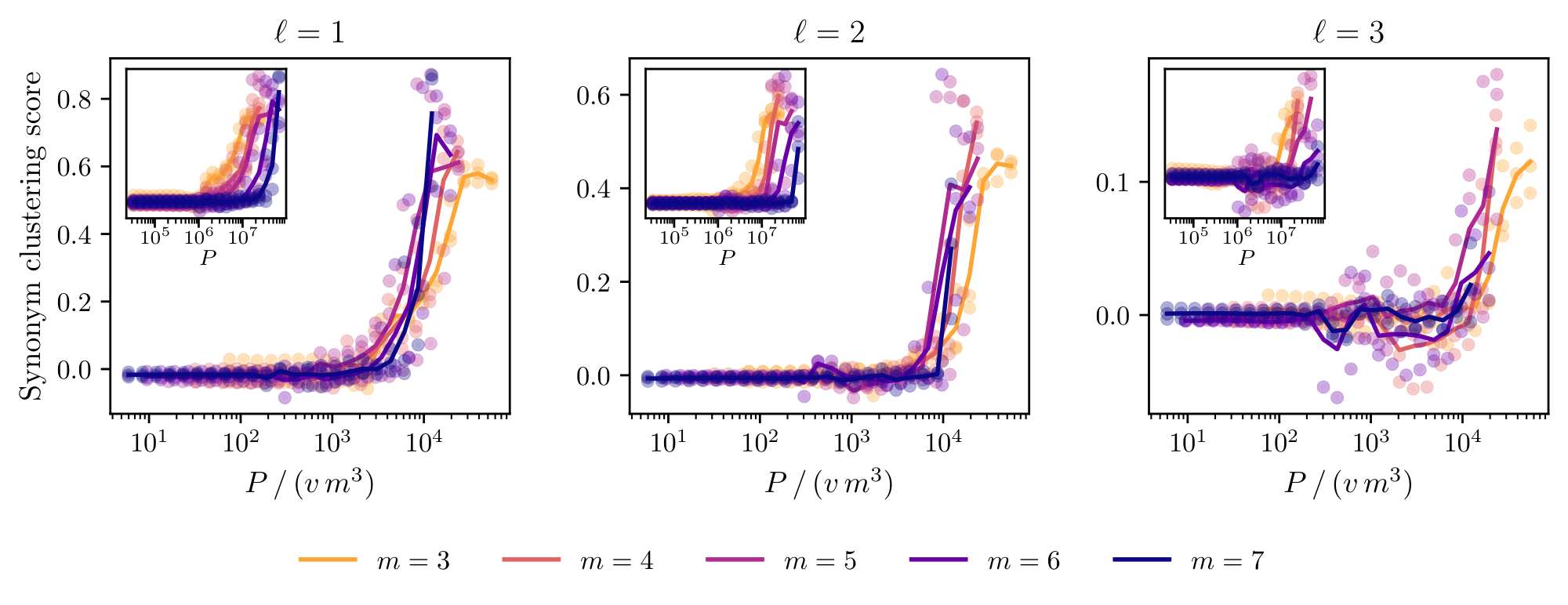
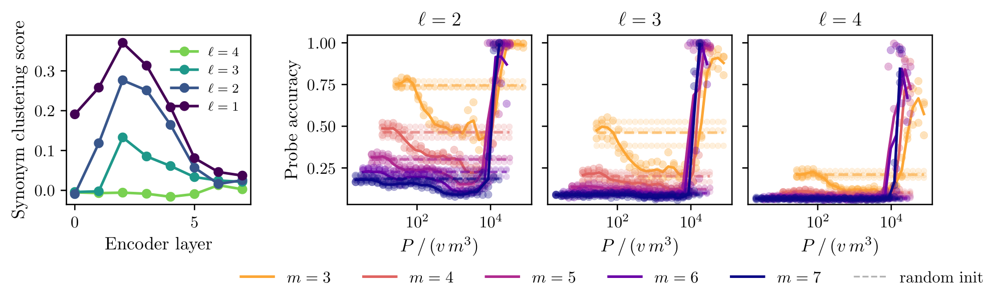
Our theoretical argument predicts that the data2vec encoder collapses synonymous level- $\ell$ tuples onto a common representation – the very geometric signature of clustering. We test this prediction directly by measuring the synonym clustering score $\mathcal C_\ell$ of the encoder at level $\ell$ by comparing the change in its hidden representations under two interventions on the input: a synonym swap, which resamples every level- $\ell$ production rule and thus replaces each level- $(\ell-1)$ tuple by a synonym while leaving higher-level latents unchanged, and a generic swap to an unrelated input. The score is normalized so that $\mathcal C_\ell=0$ when synonym swaps move the representation as much as generic swaps (no clustering), and $\mathcal C_\ell=1$ when synonyms are mapped to a common image (perfect clustering). Figure 5 reports $\mathcal C_\ell$ at each non-root level after the third block of the encoder as a function of pretraining samples $P$. The scores at all three levels rise from zero and collapse onto a common curve once the sample axis is rescaled by $vm^3$. This is direct evidence that data2vec's encoder implements the same recursive clustering mechanism as the ILC algorithm of Section 3, with the same per-level $vm^3$ sample complexity predicted by the theory.

6. Conclusion

Section Summary: The study shows that training models to predict from their own internal latent features, rather than raw tokens, can recover the hidden hierarchical structure of synthetic data using dramatically fewer examples than standard self-supervised methods. This works because features at the same level of the hierarchy share stronger statistical relationships that get diluted when working directly with surface-level inputs. The authors discuss how this finding might help design more efficient AI training schemes, point to possible links with brain-like learning, and note the limits of testing the idea only on simple artificial languages.

We have proved that learning from one's own latents recovers the full non-root latent tree of the Random Hierarchy Model from a number of samples scaling as $m^3$, exponentially fewer than the $m^{L+1}$ required by token-level self-supervised objectives. We confirmed this prediction with a hierarchical clustering algorithm, an end-to-end neural network of predictor-clusterer modules, and the first sample-complexity analysis of data2vec. The main lesson is that latents at the same level of the hierarchy are far more correlated with each other than they are with raw tokens, so predicting from one's own latents amplifies a signal that token-level prediction dilutes. This places on a firm quantitative footing the common intuition that token-level prediction is suboptimal.

Practical implications.

Recent work supports that empirical neural scaling laws in language are governed by power-law decays of token correlations with context length ([33, 34, 38]). Can generative models trained with own-latent self-supervision systematically beat existing scaling laws, alone or in combination with token-level losses? A useful first step would be a controlled comparison between data2vec and a same-architecture next-token-prediction baseline as the training-set size $P$ is varied: at small $P$ the two should diverge sharply, while at very large $P$ they should converge to the same latent representations. Such a comparison would empirically test our central prediction and, if confirmed, motivate latent-supervised generative models as a route to break current scaling regimes.

Biological plausibility.

As we show in Appendix C.2, the predictor-clusterer modules of Section 4 can also reach the $m^3$ scaling of sample complexity using only quasilocal learning rules – stop-gradients between modules in place of end-to-end backpropagation. In this local learning setting our method is conceptually similar to contrastive predictive coding ([50]) and CLAPP ([20]), which both propose biologically plausible self-supervised objectives that predict in latent rather than raw-sensory space. This raises the question of whether the remarkable sample efficiency of the human brain stems from a similar mechanism. Very recently, CLAPP was trained on the RHM in a setting where information on the top root label was given, recovering the supervised learning sample complexity $m^L$ – see Appendix A for details. It would be interesting to test whether such bio-plausible architectures can reach a $m^3$ sample complexity on the RHM simply by learning from their own latent.

Limitations.

The RHM is a deliberately simple synthetic language: its context-free grammar has a fixed tree topology and unambiguous, non-recursive production rules. Extending the analysis to (i) variable tree topologies, (ii) recursive production rules that can call themselves, and (iii) explicitly context-dependent rules will bring the theory closer to natural language and images. Such extensions are likely important to characterize precisely the relative strengths and weaknesses of various architectures. Although our analysis suggests that stacking JEPAs as in H-JEPA is largely redundant, very recent self-supervised architectures claim explicit hierarchical supervision but are neither stacked JEPAs nor stacked data2vecs, and instead resemble data2vec-style training procedures with multi-scale teachers ([51, 52]). These architectures would be interesting to study theoretically. More broadly, developing a suite of synthetic data models will provide a laboratory in which new architectures can be designed, tested, and theoretically understood before being scaled up.

Acknowledgments

We thank Francesco Cagnetta, Francesco D'Amico, Ariane Delrocq, Antonio Sclocchi, and Wu Zihan for discussions and feedback on the manuscript, and the members of the Simons collaboration for discussions. D. J. Korchinski acknowledges financial support from the Natural Sciences and Engineering Research Council of Canada (NSERC PDF - 587940 - 2024). A. Favero acknowledges support from the Infosys-Cambridge AI Centre. This work was supported by the Simons Foundation through the Simons Collaboration on the Physics of Learning and Neural Computation (Award ID: SFI-MPS-POL00012574-05), PI Wyart.

Appendix

Section Summary: This appendix extends discussions of related research on hierarchical generative models, approximation bounds, and self-supervised learning methods—including clustering-based approaches like DeepCluster and DINO, as well as architectures such as H-JEPA, Bootleg, and predictive coding models—while comparing their capabilities for learning structured data like regular hierarchical languages. It then presents a technical proof establishing recovery guarantees for an iterative latent clustering algorithm. The proof relies on assumptions about balanced, well-separated grammars and stable clustering modules to show that the method can accurately recover hierarchical structure from samples.

A. Further related work

Approximation- and information-theoretic bounds.

Deep networks can represent hierarchically compositional functions with exponentially fewer parameters than shallow ones ([40]), which translates into nonparametric sample-complexity bounds polynomial in the input dimension for both supervised ([41]) and self-supervised ([42]) tasks. These results characterize expressivity and information-theoretic statistics, but do not describe what gradient descent can actually learn from a finite training set.

Supervised learning.

[46] introduced phylogeny-inspired generative models on regular trees, and [47] showed that they can be learned by an iterative clustering algorithm. [48] introduced languages with random production rules. The RHM ([32]) combines both assumptions, leading to models with controllable correlations where sample complexity can be predicted and compared to observations in deep nets. [53] proved rigorously that result for multi-step gradient descent. [54] obtains sample complexity for non-regular trees. [55] derive optimal scaling laws for hierarchical multi-index models, a related class of generative models with continuous latents.

Self-supervised learning.

A complementary line of work has shown that transformers can approximately implement parsing-style (inside-algorithm) inference on context-free grammars ([43, 44, 45]). These results interpret the algorithm that trained LLMs implement, but do not characterize the learning mechanism nor its sample complexity. Such analyses do exist for the RHM, but only for next-token prediction ([32]) and for diffusion ([38, 37]), not for learning from one's own latents as considered here.

Clustering-based approaches to self-distillation.

Our SLC method is similar in spirit to clustering or self-learned pseudo-labeling-based methods for image-representation learning, such as DeepCluster [56] which in turn evolved into SwAV [57], the DINO family of models [23, 58, 59], iBOT [60], and CAPI [61]. Our method adds explicit hierarchical clustering – it would be interesting to test to what degree implicit hierarchical supervision is present for these clustering-based approaches.

Explicitly hierarchical self-distillation SSL.

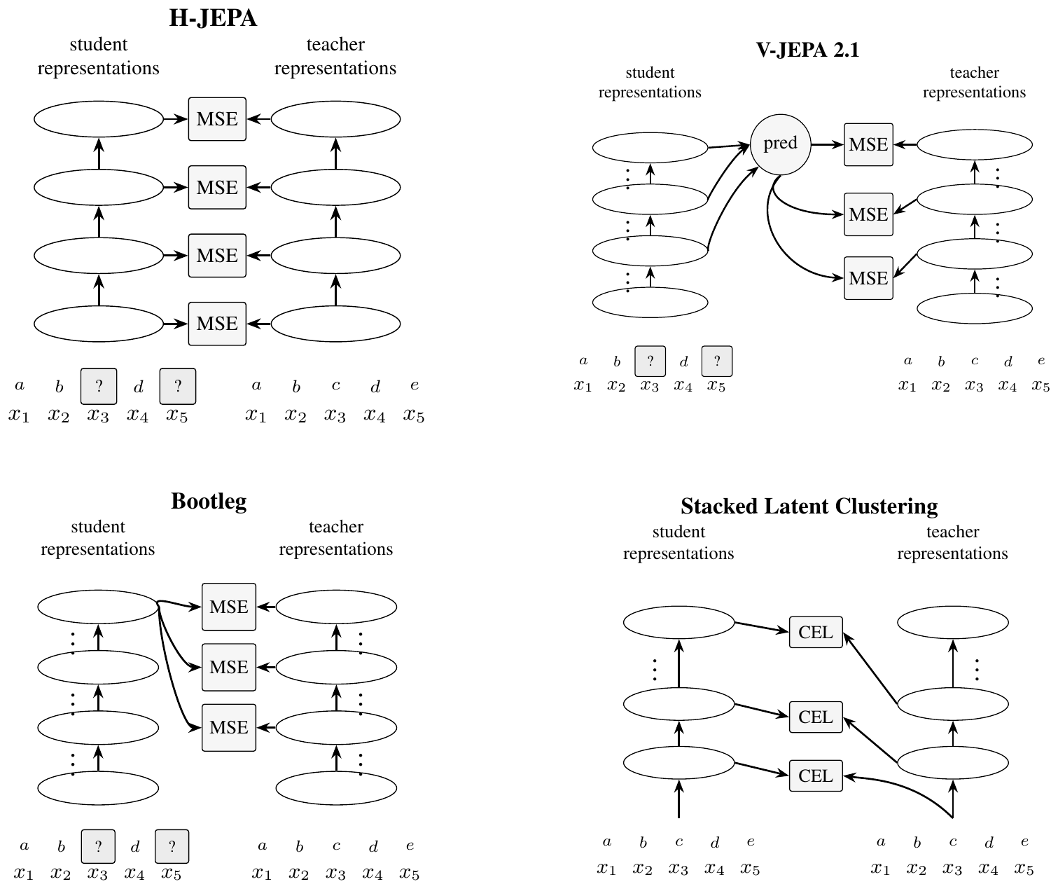
Schematic realizations of the H-JEPA [17], V-JEPA 2.1 [62], Bootleg [51], and our SLC architectures are depicted in Figure 6. Bootleg and V-JEPA 2.1 are extremely recent, report state of the art performance, and employ multi-loss optimization with one prediction per sampled representation level. Bootleg is schematically very similar to data2vec (cf. Figure 4–left), except that in bootleg gradients are computed after averaging losses over representations, whereas in data2vec the averaging is done first over representations. V-JEPA 2.1 meanwhile collates representations from throughout the student network, similar to H-JEPA, but also allows low-level target predictions to be influenced by higher level latents. This high $\rightarrow$ low prediction path is missing in H-JEPA, but present in SLC, V-JEPA 2.1, and Bootleg. It is important to clarify whether this is related to the fact that, with few exceptions [26, 27], "standard" H-JEPA appears to have found limited application in the literature.

Predictive coding and the RHM.

[63] recently showed that a backprop-free predictive coding model, CLAPP, can learn the RHM's hierarchical structure with sample complexity comparable to that of backprop. In that work, the model was trained on the RHM in the setting where all production rules exist, such that all sentences belong to the language (corresponding to $f=1$ in our notations). In that case, self-supervised methods cannot learn the RHM rules, as all inputs are equiprobable and correlations within the input are absent. However, the variation of CLAPP considered in that work uses a contrastive update rule that is gated by an extra learning signal: updates are given a $\pm 1$ sign indicating whether pairs belong to the same top-level class. The sample complexity obtained was that of supervised learning $\sim m^L$. Baseline CLAPP [20] does not rely on this non-local context supervision – it would be interesting to understand whether it learns the RHM rules in sample complexity $m^3$ when $f<1$.

**Figure 6:** **Top left:** Structure of losses and targets for naïve H-JEPAs. **Top right:** Structure of losses and targets in V-JEPA 2.1. **Bottom left:** Structure of losses and targets for Bootleg. **Bottom right:** A schematic implementation of Stacked Latent Clustering, in which high-level representations are grounded in predicted lower-level representations.

B. Proof of Iterative Latent Clustering recovery

This appendix proves the recovery guarantee for Iterative Latent Clustering. Throughout the proof, probabilities are taken over fresh samples from a fixed grammar instance, unless an expectation over grammars is explicitly denoted by $\mathbb E_{\mathcal G}$ .

B.1 Formal assumptions

We use the following two assumptions. The first is a typical-event assumption on the random grammar. The second is an algorithmic stability assumption on the clustering module.

########## {caption="Assumption 2: Balanced and separated grammar"}

There exist constants $c_{bal}, C_{bal}, c_{sep}>0$, independent of $v, m, L$, such that for every level $\ell=0, \ldots, L-2$, every grammatical tuple $\nu\in\mathcal S_\ell$ satisfies

$ \frac{c_{bal}}{vm}\leq \mathbb P[T=\nu]\leq \frac{C_{bal}}{vm}, $

and the parent context vectors satisfy

$ \min_{a\neq b}|\Phi_{\ell, a}-\Phi_{\ell, b}|2\geq c{sep}\frac{\sqrt{1-f}}{m}. $

########## {caption="Assumption 3: Stable clustering module"}

Let ${z_\nu:\nu\in\mathcal S_\ell}\subset\mathbb R^v$ be points with true centers ${\Phi_{\ell, a}:a\in\mathcal V_{\ell+1}}$ . Suppose that

$ |z_\nu-\Phi_{\ell, \mathrm{par}_\ell(\nu)}|_2\leq \varepsilon $

for all $\nu\in\mathcal S_\ell$, and that

$ |\Phi_{\ell, a}-\Phi_{\ell, b}|_2\geq \Delta $

for all $a\neq b$ . If $\varepsilon\leq \Delta/8$, then $\mathsf{Cluster}v({z\nu}{\nu\in\mathcal S\ell})$ returns the true partition $\mathcal S_\ell=\bigsqcup_{a\in\mathcal V_{\ell+1}}\mathcal S_{\ell, a}$, up to a permutation of labels.

Assumption 2 is a high-probability random-grammar event. Balancedness follows from asymptotic uniformity of single-symbol marginals in the limit $v\to\infty$ at fixed $f\in(0, 1)$, see Lemma C.1 of [54]. Indeed, if $\nu\in\mathcal S_{\ell, a}$, then $\nu$ is generated with probability $1/m$ conditional on its parent $a$ . Therefore

$ \mathbb P[T^{(\ell)}=\nu]

\frac1m\mathbb P[h^{(\ell+1)}=a] \sim \frac1{vm}. $

The separation scale is the latent-latent correlation scale. Indeed, writing

$ \psi_\ell(\nu):=\phi_\ell(\nu)-\mathbb E[e_Y], $

the connected covariance column is

$ C_\ell(:, \nu)=\mathbb P[T=\nu]\psi_\ell(\nu). $

For $\ell=0$, $T$ is a grammatical visible $s$ -tuple and $Y$ is a visible token in a sibling branch, with lowest common ancestor two levels above the leaves. This is precisely the token–tuple covariance computed in [33]. In our notation, their calculation gives, for a fixed visible value $y$ and a grammatical tuple $\nu$,

$ \mathbb E_{\mathcal G}!\left[C_0(y, \nu)^2, \middle|, \nu\in\mathcal S_0\right]\asymp \frac{1-f}{v^3m^4}. $

Summing over the $v$ possible values of $Y$ yields the squared column norm

$ \mathbb E_{\mathcal G}!\left[|C_0(:, \nu)|_2^2, \middle|, \nu\in\mathcal S_0\right]\asymp v\cdot \frac{1-f}{v^3m^4}=\frac{1-f}{v^2m^4}. $

The same estimate holds at every latent level by self-similarity of the RHM. Indeed, fix $\ell>0$ and consider the sequence of level- $\ell$ variables

$ H^{(\ell)}:=\big(h^{(\ell)}1, \ldots, h^{(\ell)}{s^{L-\ell}}\big). $

Marginally, $H^{(\ell)}$ is generated by an RHM of depth $L-\ell$ with the same local parameters $(s, v, m)$, using the production rules at levels $\ell, \ell+1, \ldots, L-1$ . In this truncated RHM, the level- $\ell$ variables play the role of visible tokens. Our statistic $C_\ell(:, \nu)$ is therefore exactly the level- $0$ token–tuple covariance of this truncated model: $T$ is a terminal $s$ -tuple, $Y$ is a terminal child in a sibling branch, and their lowest common ancestor is again two levels above the terminal scale. Since the random rule ensemble has the same law at every level, the same covariance calculation gives

$ \mathbb E_{\mathcal G}!\left[|C_\ell(:, \nu)|2^2, \middle|, \nu\in\mathcal S\ell\right]\asymp \frac{1-f}{v^2m^4}, $

uniformly for $\ell=0, \ldots, L-2$ . Since

$ C_\ell(:, \nu)=\mathbb P[T=\nu]\psi_\ell(\nu) $

and, on the balancedness event, $\mathbb P[T=\nu]\asymp 1/(vm)$, this implies

$ \mathbb E_{\mathcal G}!\left[|\psi_\ell(\nu)|2^2, \middle|, \nu\in\mathcal S\ell\right]\asymp \frac{(1-f)/(v^2m^4)}{1/(v^2m^2)}=\frac{1-f}{m^2}. $

Thus $\sqrt{1-f}/m$ is the natural scale of the centered context-vector signal.

To turn this into a separation statement, we need to assume that different parent context vectors have generic relative positions, as expected for independent random production rules. In particular, under a random-direction heuristic, overlaps are smaller than squared norms by a factor $v^{-1/2}$, so pairwise distances have the same scale as the individual norms.

B.2 Theorem and proof

########## {caption="Theorem 4: Recovery of the non-root hierarchy"}

Assume the balancedness and separation conditions above, and assume the clustering is stable under perturbations as described. Then there exists a constant $C>0$, depending only on the constants in those assumptions and on $s$, such that the following holds. If

$ P \geq C \left[vm\log\frac{Lvm}{\delta} + \frac{v m^3}{1-f} \log\frac{Lvm}{\delta} \right], $

In particular, up to logarithmic factors, $P_{ILC} \asymp (1-f)^{-1} , v m^3.$

Synonyms have identical context vectors.

We first record the property that makes clustering possible.

########## {caption="Lemma 5: Synonyms have identical context vectors"}

If $\nu, \nu'\in\mathcal S_\ell$ satisfy $par_\ell(\nu)=par_\ell(\nu')$, then $\phi_\ell(\nu)=\phi_\ell(\nu')$ .

Proof: Let $A$ be the level- $(\ell+1)$ parent of the branch containing $T$, let $B$ be the level- $(\ell+1)$ parent of the sibling branch containing $Y$, and let $G$ be their shared level- $(\ell+2)$ parent. The local graphical structure is $G\to(A, B)$, $A\to T$, and $B\to Y$ . By unambiguity, observing $T=\nu$ determines $A=par_\ell(\nu)$ . By the context-free Markov structure, conditioned on $A$, the rest of the tree is independent of which production rule was used to generate $T$ . Hence, if $\nu\in\mathcal S_{\ell, a}$,

$ \mathbb P[Y=y\mid T=\nu]=\mathbb P[Y=y\mid A=a]. $

The right-hand side depends on $\nu$ only through its parent $a$ . Therefore all tuples in the same synonym class have the same context vector.

Concentration of empirical context vectors.

Fix a level $\ell$ and a grammatical tuple $\nu\in\mathcal S_\ell$ . Let $N_\nu$ be the number of samples in which the chosen cousin tuple equals $\nu$, and let $Y_1, \ldots, Y_{N_\nu}$ be the corresponding target values. Conditional on $T=\nu$, these are independent draws from the conditional law of $Y$, and the empirical context vector

$ \widehat\phi_\ell(\nu)=\frac1{N_\nu}\sum_{q=1}^{N_\nu} e_{Y_q} $

is the empirical mean of $N_\nu$ independent one-hot vectors with mean $\phi_\ell(\nu)=\mathbb E[e_Y\mid T=\nu]$ .

########## {caption="Lemma 6: Context-vector concentration"}

There is a constant $C_0>0$ such that, for any $\eta\in(0, e^{-1}]$,

$ \mathbb P!\left[|\widehat\phi_\ell(\nu)-\phi_\ell(\nu)|2>C_0\sqrt{\frac{\log(1/\eta)}{N\nu}}, \middle|, N_\nu\right]\leq \eta. $

Proof: Condition on $N_\nu=n\geq1$ . Define

$ U_q:=e_{Y_q}-\phi_\ell(\nu), \qquad \bar{U}:=\frac1n\sum_{q=1}^n U_q. $

Then $\mathbb E[U_q]=0$ and

$ \widehat\phi_\ell(\nu)-\phi_\ell(\nu)=\bar{U}. $

Since the $U_q$ 's are independent and mean zero, the cross terms vanish, and

$ \begin{aligned} \mathbb E|\bar{U}|2^2 &= \mathbb E\left| \frac1n\sum{q=1}^n U_q \right|2^2 \ &= \frac1{n^2}\sum{q=1}^n \mathbb E|U_q|_2^2 \ &\leq \frac1n, \end{aligned} $

where we used

$ \mathbb E|e_Y-\phi_\ell(\nu)|_2^2

1-|\phi_\ell(\nu)|_2^2 \leq 1. $

Thus,

$ \mathbb E|\bar{U}|_2\leq n^{-1/2}. $

Now consider the function

$ F(Y_1, \ldots, Y_n):=|\bar{U}|_2. $

Changing one observation changes $\bar{U}$ by at most $\sqrt2/n$, and hence changes $F$ by at most $\sqrt2/n$ . By McDiarmid's bounded-differences inequality,

$ \mathbb P!\left[F-\mathbb EF>t \right] \leq \exp(-n t^2). $

Taking

$ t=\sqrt{\frac{\log(1/\eta)}{n}}, $

we get, with probability at least $1-\eta$,

$ F \leq \frac1{\sqrt n} + \sqrt{\frac{\log(1/\eta)}{n}}. $

Since $\eta\leq e^{-1}$, we have $\log(1/\eta)\geq1$, so the first term is absorbed into the second. Thus, for a constant $C_0$,

$ |\widehat\phi_\ell(\nu)-\phi_\ell(\nu)|_2

|\bar{U}|_2 \leq C_0\sqrt{\frac{\log(1/\eta)}{n}} $

with probability at least $1-\eta$ .

Proof of the theorem.

At each level $\ell$, let $T_\ell$ be the level- $\ell$ tuple to be clustered and $Z_\ell$ the level- $\ell$ target in the sibling branch. For sample $p$, denote the corresponding true variables by $T_\ell^{(p)}$ and $Z_\ell^{(p)}$

We now prove Theorem 4.

Proof of Theorem 4: We first define a good event using the true latent variables. For every level $\ell=0, \ldots, L-2$ and every grammatical tuple $\nu\in\mathcal S_\ell$, let

$ N_{\ell, \nu}:=\sum_{p=1}^P \mathbf 1{T_\ell^{(p)}=\nu} $

be the number of samples in which the true level- $\ell$ cousin tuple equals $\nu$, and let

$ \widetilde\phi_\ell(\nu):= \frac{1}{N_{\ell, \nu}}\sum_{p=1}^P e_{Z_\ell^{(p)}}\mathbf 1{T_\ell^{(p)}=\nu} $

be the corresponding oracle empirical context vector.

By balancedness,

$ \mathbb P[T_\ell=\nu]\geq \frac{c_{bal}}{vm}. $

Thus $N_{\ell, \nu}$ is binomial with mean at least $c_{bal}P/(vm)$ . A Chernoff bound and a union bound over all $(L-1)vm$ pairs $(\ell, \nu)$ imply that, if

$ P\gtrsim vm\log\frac{Lvm}{\delta}, $

then, with probability at least $1-\delta/2$,

$ N_{\ell, \nu}\gtrsim \frac{P}{vm} $

simultaneously for all $\ell$ and $\nu$ .

On this count event, Lemma 6, applied with $\eta=\delta/(2Lvm)$, and another union bound give

$ \max_{\ell, \nu} |\widetilde\phi_\ell(\nu)-\phi_\ell(\nu)|_2 \lesssim \sqrt{\frac{vm}{P}\log\frac{Lvm}{\delta}} $

with probability at least $1-\delta/2$ . Therefore, if

$ P\gtrsim \frac{vm^3}{1-f}\log\frac{Lvm}{\delta}, $

then, with probability at least $1-\delta$,

$ |\widetilde\phi_\ell(\nu)-\phi_\ell(\nu)|2 \leq \frac18 c{sep}\frac{\sqrt{1-f}}{m} $

for all $\ell$ and all $\nu\in\mathcal S_\ell$ . Call this simultaneous event $\mathcal E$ .

We now show that on $\mathcal E$, the algorithm succeeds deterministically. At level $0$, the variables are visible tokens, so $\widehat{h}^{(0)}=h^{(0)}$ . Suppose inductively that level $\ell$ has been recovered exactly, up to a permutation of labels. Then the recovered level- $\ell$ tuples are the true level- $\ell$ tuples, up to relabeling. Consequently, the empirical context vectors computed by the algorithm are exactly the oracle vectors $\widetilde\phi_\ell(\nu)$, up to permutations of tuple labels and output coordinates. These permutations preserve distances.

Thus, on $\mathcal E$, every empirical context vector lies within

$ \frac18 c_{sep}\frac{\sqrt{1-f}}{m} $

of its true parent center. By separation,

$ \min_{a\neq b}|\Phi_{\ell, a}-\Phi_{\ell, b}|2 \geq c{sep}\frac{\sqrt{1-f}}{m}. $

The stable clustering assumption therefore implies that the clustering step recovers the true synonym partition

$ \mathcal S_\ell

\bigsqcup_{a\in\mathcal V_{\ell+1}}\mathcal S_{\ell, a} $

up to a permutation of labels. Assigning each tuple to its cluster recovers level $\ell+1$, again up to a permutation of labels.

Iterating this deterministic induction from $\ell=0$ to $L-2$ recovers $h^{(1)}, \ldots, h^{(L-1)}$ and all production-rule classes below the root. Since $\mathcal E$ holds with probability at least $1-\delta$, the theorem follows.

The required sample size is

$ P\gtrsim vm\log\frac{Lvm}{\delta} + \frac{vm^3}{1-f}\log\frac{Lvm}{\delta}. $

Thus, up to logarithmic factors, $P \gtrsim vm^3/(1-f)$ suffices for recovery, and we write

$ P_{ILC}\asymp \frac{vm^3}{1-f} $

for this threshold.

C. Stacked latent-clustering details and additional results

This appendix gives implementation details and additional diagnostics for the SLC network introduced in Section 4. We use the RHM notation of Section 2: true latent variables are denoted by $h^{(\ell)}_i$, while learned SLC tokens are denoted by $\widehat{h}^{(\ell)}_i$.

C.1 SLC architecture details

We encode RHM input strings of size $s^L$ into one-hot feature vectors of dimension $\mathbb{R}^{s^L \times d_h}$, where $d_h \gg v$ is the dimension into which we tokenize learned latents. This initializes the level- $0$ tokens as $\widehat{h}^{(0)}_i=x_i$. We use a single dimension $d_h$ for the cluster codebook and for the token vocabulary passed between SLC modules: each clusterer assigns labels in ${1, \ldots, d_h}$, these labels become the tokens for the next module, and predictors therefore output categorical distributions over $d_h$ token identities.

A SLC model for an RHM of depth $L$ is comprised of $L-1$ SLC modules. Module $\ell$ reduces the learned level- $\ell$ sequence to an encoding of the level- $(\ell+1)$ latents. For a module at level $\ell$, the tensor shapes are

$ \begin{array}{rcl} \widehat{h}^{(\ell)} &\in& \mathbb R^{s^{L-\ell}\times d_h}, \ x_u^{(\ell)} := \big(\widehat{h}^{(\ell)}{(u-1)s+1}, \ldots, \widehat{h}^{(\ell)}{us}\big) &\in& \mathbb R^{s\times d_h}, \ \widehat\phi^{(\ell)}_u

\mathrm{Pred}^{(\ell)}(x_u^{(\ell)}) &\in& \mathbb R^{s\times(s-1)\times s\times d_h}, \ \mathrm{vec}, \widehat\phi^{(\ell)}_u &\in& \mathbb R^{s^2(s-1)d_h}, \ q_u^{(\ell+1)}

\mathrm{Clust}^{(\ell)}(\mathrm{vec}, \widehat\phi^{(\ell)}_u) &\in& \Delta^{d_h-1}, \ \widehat{h}^{(\ell+1)} &\in& \mathbb R^{s^{L-\ell-1}\times d_h}. \end{array} $

Here $u=1, \ldots, s^{L-\ell-1}$ indexes level- $\ell$ patches, and $d_{h_2}$ is the hidden width of the CNN layers below. The dimensions of $\widehat\phi^{(\ell)}_u$ enumerate, respectively, the possible position of the input patch within its grandparent, the target cousin patch, the target token within that patch, and the $d_h$ token identity. This task is easiest for $d_h = v$, as clustering is architecturally enforced, and is hardest for $d_h\ge mv$ (when synonyms can be uniquely encoded without clustering). Unless otherwise noted, we will always use $d_h=mv$.

A SLC module is composed of a predictor and a clusterer. This arrangement is depicted in Figure 7.

**Figure 7:** **Schematic of a single SLC module, with the layer-wise prediction and clustering losses.**

**Figure 8:** **Multiple predictions improve signal**. We train the predictor and clusterer modules with weight sharing, and train cross-entropy prediction at all possible positions and cousin targets.

Predictor.

The predictor operates on an $s$-tuple patch and predicts all $s(s-1)$ tokens with the same grandparent (cf. Figure 8 for a visualization). Using all cousin targets increases the available signal and improves prefactors, although it does not change the asymptotic sample-complexity scaling. Because the same patch can occupy any of the $s$ positions under its grandparent and we use weight sharing across positions, the predictor outputs $s^2(s-1)$ distributions; for each observed patch, only the $s(s-1)$ distributions matching its actual position enter the loss. The predictor is implemented in terms of convolutional layers, as

$ \widehat\phi^{(\ell)}(x) = \mathrm{Pred}^{(\ell)}(x) = (\operatorname{\mathrm{SM}}\circ \operatorname{\mathrm{CNN}}_3 \circ A\circ \operatorname{\mathrm{CNN}}_2 \circ A \circ \operatorname{\mathrm{CNN}}_1)(x) $

where $A = \operatorname{\mathrm{ReLU}} \circ \mathrm{BN}$ denotes the activation function, $\operatorname{\mathrm{CNN}}1 : \mathbb{R}^{s\times d_h} \rightarrow \mathbb{R}^{d{h_2}}$ is a stride $s$ 1d convolutional layer, while $\operatorname{\mathrm{CNN}}2 : \mathbb{R}^{ d{h_2}} \rightarrow \mathbb{R}^{d_{h_2}}$ and $\operatorname{\mathrm{CNN}}3 : \mathbb{R}^{d{h_2}}\rightarrow \mathbb{R}^{s\times (s-1)\times s \times d_h}$ are both stride 1. The softmax operation $\operatorname{\mathrm{SM}}$ acts on the last dimension so that $\sum_{a=1}^{d_h} \widehat\phi^{(\ell)}(x)_{r\rho ta} =1 $. This last dimension is therefore the marginal probability distribution over neighbouring tokens, conditioned on the input patch position $r$, target cousin-patch index $\rho$, and target token position $t$.

We train the predictor with a cross-entropy prediction loss. Fix a grandparent index $g\in{1, \ldots, s^{L-\ell-2}}$ and an input patch position $r\in{1, \ldots, s}$ within that grandparent, so that $u=(g-1)s+r$ and the input patch is $x_u^{(\ell)}$. For a target cousin patch position $r'\ne r$, let $\rho_r(r')\in{1, \ldots, s-1}$ denote the index of $r'$ among the patch positions excluding $r$. The level- $\ell$ token at target position $t$ inside target patch $r'$ has absolute index

$ i(g, r', t):=((g-1)s+r'-1)s+t . $

For this input patch, the prediction loss is

$ \mathcal{L}_\mathrm{pred}(g, r)

-\sum_{r'\ne r}\sum_{t=1}^s \sum_{a=1}^{d_h} \widehat{h}^{(\ell)}{i(g, r', t), a} \log!\left(\widehat\phi^{(\ell)}(x_u^{(\ell)}){r, \rho_r(r'), t, a} \right). $

The predictor loss for module $\ell$ is the mean of this quantity over all grandparent indices $g$ and input patch positions $r$.

Clusterer.

The clusterer in turn assigns soft cluster labels to each patch's prediction vector – this amounts to assigning a learned level- $(\ell+1)$ latent label.

$ q^{(\ell+1)} = \mathrm{Clust}^{(\ell)}(\widehat\phi^{(\ell)}) = (\operatorname{\mathrm{SM}} \circ \operatorname{\mathrm{CNN}}_5 \circ A \circ \operatorname{\mathrm{CNN}}_4)(\widehat\phi^{(\ell)}) $

where $\widehat\phi^{(\ell)}$ denotes the flattened output of $\mathrm{Pred}^{(\ell)}$, $\operatorname{\mathrm{CNN}}4 : \mathbb{R}^{s^2(s-1)d_h} \rightarrow \mathbb{R}^{d{h_2}} $ and $\operatorname{\mathrm{CNN}}5 : \mathbb{R}^{d{h_2}} \rightarrow \mathbb{R}^{d_h} $ are stride-1 CNNs. The soft code $q^{(\ell+1)}$ is the learned token $\widehat{h}^{(\ell+1)}$ passed to the next module. A priori we do not specify that $d_h = v$, so the clusterer could choose to instead assign each synonym of a patch into its own cluster. Indeed, for finite data, differing but synonymous patches will imply different contexts due to finite sampling effects. We address this by using a contrastive clustering loss that penalizes assignments of sufficiently similar predictions into different clusters.

Let $q_i = \mathrm{Clust}^{(\ell)}(\widehat\phi^{(\ell)}_i)$ denote the soft cluster assignment for prediction vector $\widehat\phi^{(\ell)}_i$, where the index $i$ is taken to be over patch positions and batches, and we drop the $^{(\ell)}$ superscript for brevity. The predictions are then centred, so that $\widehat\phi^{(\ell)}_i \rightarrow \widehat\phi^{(\ell)}_i - \langle \widehat\phi^{(\ell)}j \rangle_j$. The similarity $S{ij}$ between two predictions is the scaled cosine similarity

$ S_{ij} = \frac{1}{2}\left(1+\frac{\widehat\phi^{(\ell)}_i\cdot\widehat\phi^{(\ell)}_j}{||\widehat\phi^{(\ell)}_i||_2||\widehat\phi^{(\ell)}_j||_2}\right) $

of these centred predictions. The clustering loss is then

$ \mathcal{L}\mathrm{clust} = \langle \mathcal{L}\mathrm{sim}(q_i, q_j, S_{ij}) + \lambda_{\mathrm{sep}}\mathcal{L}\mathrm{sep}(q_i, q_j, S{ij})\rangle_{ij} + \lambda_\mathrm{sparsity} \langle \mathcal{L}_\mathrm{sparsity}(q_i)\rangle_i $

where the $\langle \cdot\rangle_{ij}$ indicates an average over patch positions and batches. The similarity loss component

$ \mathcal{L}\mathrm{sim}(q_i, q_j, S{ij}) = (q_i-q_j)\cdot(q_i-q_j)\operatorname{\mathrm{ReLU}}(S_{ij} - S_{m}) $

serves to penalize predictions that are sufficiently similar (more than the margin $S_m$) but assigned to different clusters (i.e. with non-zero $\Delta q$) – this loss ensures that clusters consist of similar predictions. Alone, of course, the model could simply cluster ALL predictions into a single cluster. Therefore, we include a separation loss

$ \mathcal{L}{\mathrm{sep}}(q_i, q_j, S{ij}) = q_i\cdot q_j(1-S_{ij}) $

which penalizes dissimilar (i.e. large $1-S_{ij}$) predictions that are assigned into overlapping clusters (i.e. $q_i\cdot q_j > 0$). Finally, we introduce

$ \mathcal{L}_\mathrm{sparsity}(q_i) = -q_i\cdot q_i $

which tends to maximize the $L_2$ norm of the cluster assignment and therefore the sparsity (since $||q_i||_1 = 1$ due to the softmax). Preliminary experiments demonstrated that this sparsity reward improves training stability and downstream interpretability.

A general caveat of employing contrastive losses is that memory costs can explode. Employed naïvely, the first SLC module would compute $s^{2(L-1)}$ comparisons, each of which involves a potentially costly dot-product of a $s^2(s-1)d_h$ vector. In practice for each batch, we select a random subset of $N_\mathrm{compare}$ patch positions and batches on which to compute the clustering loss for memory constraints.

Training protocol and stabilizers.

To keep the prediction problem at depth $\ell$ comparable to the prediction problem at depth $0$, we tokenize clusterer outputs by means of a softmax operation, $\operatorname{\mathrm{SM}}(X, T) = \exp(X/T)/\sum_i\exp(X_i/T)$. For $T=0$, this is hard label assignment. Preliminary experiments found that $T<1$ can improve convergence, but here we report results for $T=1$.

The clustering codebook dimension $d_h$ is another important stabilizer. If the space of possible labels is large, each input can be assigned a unique label; this is a failure to cluster, because synonyms of a latent are not assigned the same symbol in the next layer. The input vocabulary for layer $\ell+1$ then increases by a factor $m$, making the prediction task for layer $\ell+1$ intractable. This problem is exacerbated by noisy or finite sampling, where synonymous inputs do not produce identical predictions. This can be resolved by an architectural bottleneck, i.e. setting $d_h = v$, as is done for the ILC. For most natural data, this dimension is unknown a priori; to simulate these conditions we set the label dimension to $d_h>mv$ (the hardest case) and instead use the contrastive loss to set the scale of attraction between similar predictions.

To mitigate representation collapse, we use a teacher-student framework, in which latent targets are obtained from a teacher network whose weights are simply the exponentially lagged weights of the student. After each step of gradient descent, the teacher weights $W^{(T)}$ are updated towards the student weights $W^{(S)}$ with $W^{(T)} \leftarrow (1-\alpha_\mathrm{ema})W^{(T)} + \alpha_\mathrm{ema} W^{(S)}$, where $1/\alpha_\mathrm{ema}$ sets the exponential moving average timescale. The prediction loss therefore uses teacher representations to obtain targets $x_{:}$, which are evaluated against student predictions. The clustering loss meanwhile, computes the similarity $S_{ij}$ using the teacher's predictions and subsequently uses the student's clustering assignments $q_i$, $q_j$. As an alternative to the teacher-student framework, we highlight in Appendix C.2 that collapse can also be overcome by introducing stop-gradients between SLC modules, effectively making learning entirely local, reminiscent to predictive coding. Finally, we perform Jacobian descent, computing the gradient for each loss independently, and aggregate the gradients by means of the UPGrad algorithm. This selects an update in the dual-cone of the gradients to avoid conflicting updates [64], which we found in preliminary experiments reduced the need for careful hyperparameter selection.

Unless otherwise specified, SLC models are trained using AdamW and Jacobian descent (via TorchJD and UPGrad ([64])) and following hyperparameters: $\alpha_\mathrm{ema} = 0.015$, $\mathrm{lr}=$ 3 x 10^-3, $\mathrm{wd} = 10^{-3}$, $d_{h_2} = 150$, batch size 32, clustering dimension $d_h=128$, $S_m = 0.8$, $\lambda_\mathrm{sep} = 0.5$, $N_\mathrm{compare}=300$, and $\lambda_\mathrm{spars} = 10^{-2}$. These were optimized by hyperparameter sweeps conducted at $L=5$ for $v=16$, $m=8$, $s=3$ using Optuna's Tree-Parzen-Estimator sampler and Hyperband pruner [65].

We use a validation set of 2000 samples to evaluate the model throughout training. When training classifiers on the final SLC representation, we use early stopping to select the best pretraining checkpoint and classification checkpoint based on this validation set performance, but report test set performance on a held-out test set of 2000 samples. In Figure 12 the test sets are smaller, with 1000 samples.

C.2 Training with local rules

In Figure 9, we ablate the global training machinery while also testing increasingly biologically plausible training conditions. We first prevent gradient flow between SLC layers (denoted "Layer SG" for layerwise stop-gradient), then disable the exponential moving average (EMA) teacher network, and finally disable gradient flow between the prediction and clustering submodules. These changes remove the long-range backpropagating error signal and the biologically implausible time-delayed duplicate teacher network. When disabling EMA but allowing gradients to flow from the clustering loss through to the predictor, we observe representation collapse. We credit this to the clustering loss overpowering the prediction loss: trivial predictions are easy to cluster perfectly at the expense of prediction accuracy. Preventing gradient flow between prediction and clustering networks prevents this failure mode, showing that SLC can still learn when updates are constrained to local signals.

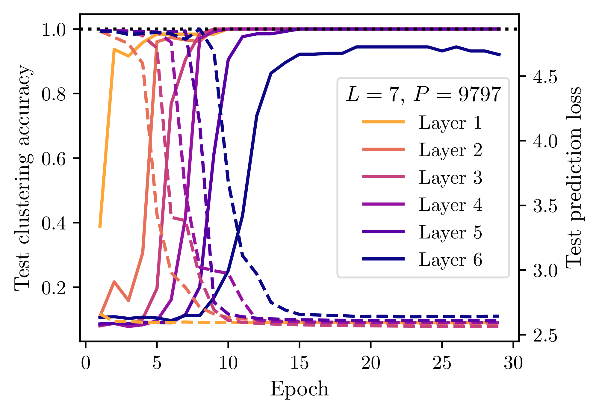
$**Figure 9:** **Local learning suffices to learn the RHM.** We compare baseline training (blue) to increasingly local learning rules. "Layer SG" in legend indicates stopgradients between SLC layers, " $P\rightarrow C$ SG" indicates stopgradient between the predictor and clusterer submodules. EMA in legend indicates exponential-moving-average teacher is used as a target. RHM parameters are: $L=4, v=10, m=10, s=3$. Solid lines are average over three independent realizations.$

C.3 Training dynamics

In Figure 10 we report the layer-wise accuracy and prediction loss of the different SLC modules. We evaluate the accuracy of module $\ell$ by taking the learned hard labels $\widehat{h}^{(\ell+1)}i$ (with the $T=0$ hard label assignment) and comparing them with the ground-truth RHM latents $h^{(\ell+1)}{i}$. We identify an optimal mapping between the assigned labellings and the true latents with the Kuhn-Munkres "Hungarian" algorithm, and report the accuracy attained with such a mapping.

**Figure 10:** **Training proceeds layer-wise.** As each layer's clustering improves, the subsequent layer's prediction loss decreases, enabling that subsequent layer to then cluster.

C.4 Independence of sample complexity with L

In Figure 11 we check that the sample complexity scaling for ILC and SLC better supports $m^3$ rather than $m^{L+1}$.

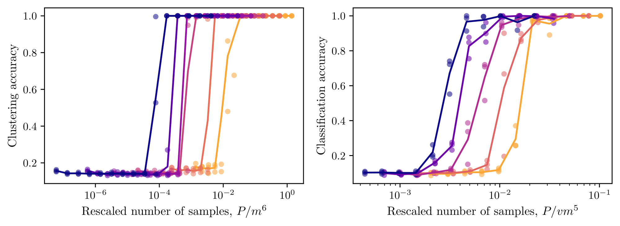
$**Figure 11:** **Attempted curve collapse with token based SSL scaling.** Data are as in Figure 3, but with the $m^{L+1}$ scaling that holds for token level SSL. The collapse of accuracy vs. training sample is significantly degraded.$

Furthermore, in Figure 12 we validate the sample complexity $P \sim m^3$ for systems with varying depth, up to $L=7$.

$**Figure 12:** **The SLC model exhibits a depth-independent sample complexity.** Accuracy of linear probes trained to classify the root latent $h^{(L)}_{1}$ from the final SLC representation. RHM parameters are $s=3$, $m=8$, and $v=16$, with depth $L$ indicated by the legend. The pre-trained models were trained for 30 epochs, and the classifiers for the same duration and on the same dataset. Solid lines are an average over three independent RHM instantiations.$

D. Further results on data2vec

Figure 13–left shows the synonym clustering score for encoder layers to latents at different depths. All layers remain invariant to $\ell=L=4$ because there is not signal for which the network can learn the root latent. For latents at level $\ell < L$, we find clustering throughout the middle layers of the network. This indicates that clustering occurs throughout the early layers of data2vec. Furthermore, the fact that for latent $\ell$ encoder layer $\ell-1$ is the first to exhibit clustering of the synonyms indicates that latents are constructed layer-by-layer. Deeper layers exhibit stronger clustering of low-level latents, up to layer 2. This inversion is reminiscent of an encoder-decoder architecture, and mimics what is observed in U-Net architectures [38].

Figure 13–right tests the presence of linear traces of latents in the teacher target for different $m$ and $\ell$. This data collapses with $vm^3$, confirming that the transition to all latents being linearly encoded in the teacher occurs at the predicted $vm^3$ scaling.

In Figure 14 we test the scaling collapse for data2vec instances trained in the offline setting, thereby decoupling the number of gradient descent steps from the number of original observed samples. We find $vm^3$ provides a good collapse.

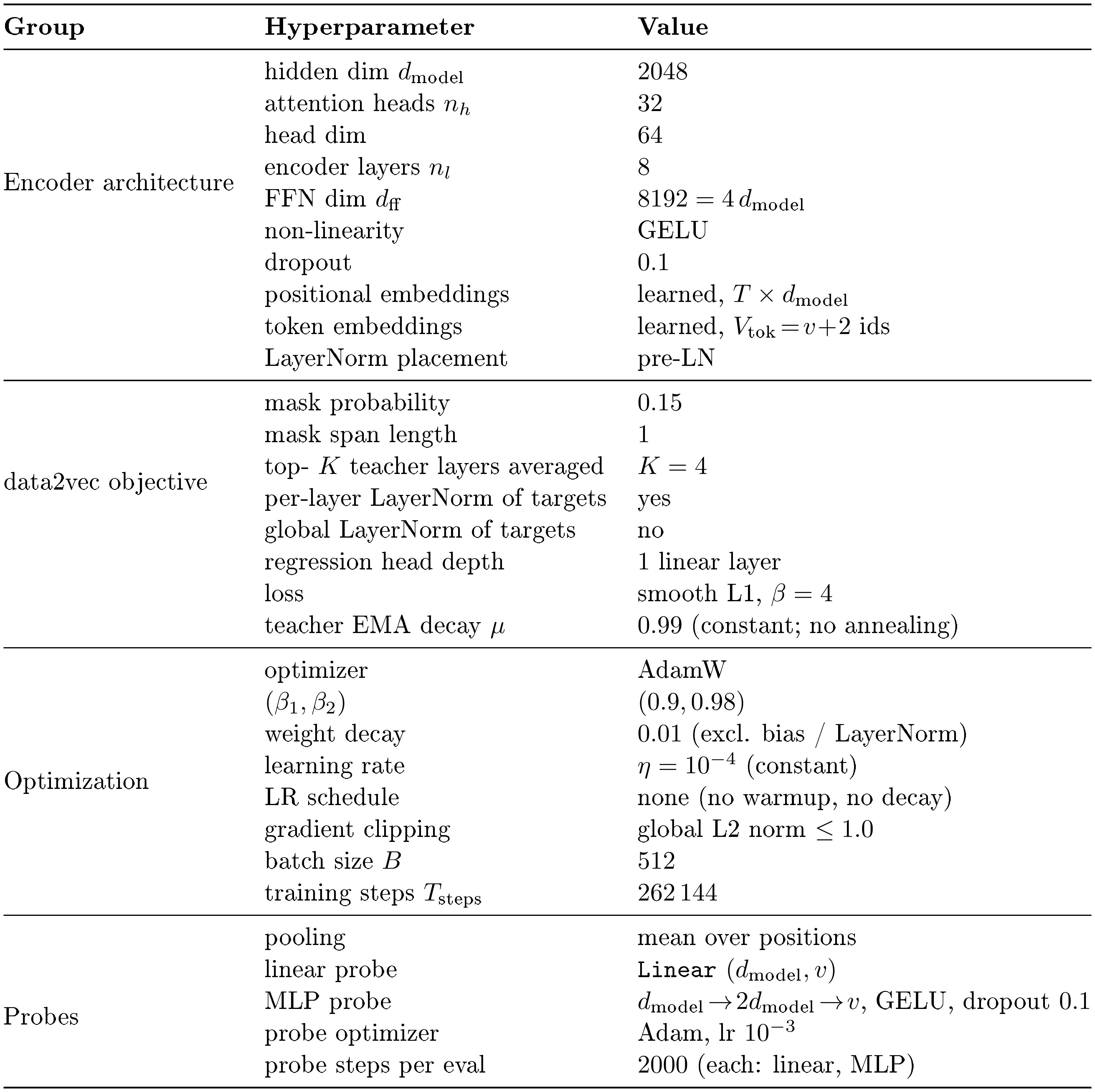
$**Figure 13:** **Left:** post-training synonym clustering score per encoder layer and RHM level $\ell$ ($m=6$). Values above $0$ indicate that synonymous level- $(\ell-1)$ tuples are clustered closer than non-synonymous ones. **Right:** linear-probe accuracy for the latent $h^{(\ell)}$ from the teacher target, vs. rescaled sample size $P/(vm^3)$, for $\ell=2, 3, 4$. Curves collapse with $vm^3$ for every $\ell$.$

**Figure 14:** **Offline data2vec pretraining.** Linear and MLP probe test accuracy on the classification task as a function of the pretraining training-set size $P$. Each point is averaged over three seeds. Main axes: curves rescaled by $vm^3$. Insets: same data, raw $P$.

::: caption="Table 1: Data2vec hyperparameters."

:::

E. Compute budget

SLC experiments were conducted on individual H100 nodes. The SLC experiments in Figure 3 took approximately 10 H100 hours. The $L$ scaling experiment reported in Figure 12 cost approximately 100 H100 hours, as the amount of computations scales linearly with input data size which consists of $ s^L$ tokens (and therefore exponentially in depth). Figure 9 cost approximately 3 H100 hours. We do not have an estimate for the Optuna hyperparameter sweeps or preliminary experiments.

The data2vec experiments cost approximately 1, 000 H100 hours.

References

Section Summary: This references section compiles citations to key academic papers and technical reports spanning artificial intelligence, machine learning, and cognitive science. It draws on foundational work about generative models for images and videos, large language models, and self-supervised learning methods, alongside studies of child language development, embodied cognition, and brain theories such as predictive coding. These sources together provide the technical and theoretical background for exploring connections between AI systems and human-like learning.

[1] Jonathan Ho, Ajay Jain, and Pieter Abbeel. Denoising diffusion probabilistic models. In Advances in Neural Information Processing Systems, 2020.

[2] Robin Rombach, Andreas Blattmann, Dominik Lorenz, Patrick Esser, and Björn Ommer. High-resolution image synthesis with latent diffusion models. In IEEE/CVF Conference on Computer Vision and Pattern Recognition (CVPR), 2022.

[3] Tim Brooks, Bill Peebles, Connor Holmes, Will DePue, Yufei Guo, Li Jing, David Schnurr, Joe Taylor, Troy Luhman, Eric Luhman, Clarence Wing Yin Ng, Ricky Wang, and Aditya Ramesh. Video generation models as world simulators. OpenAI Technical Report, 2024. URL https://openai.com/research/video-generation-models-as-world-simulators.

[4] Tom B. Brown, Benjamin Mann, Nick Ryder, Melanie Subbiah, Jared Kaplan, Prafulla Dhariwal, Arvind Neelakantan, et al. Language models are few-shot learners. In Advances in Neural Information Processing Systems, 2020.

[5] OpenAI. GPT-4 technical report. arXiv preprint arXiv:2303.08774, 2023.

[6] DeepSeek-AI. DeepSeek-R1: Incentivizing reasoning capability in LLMs via reinforcement learning. arXiv preprint arXiv:2501.12948, 2025.

[7] Jordan Hoffmann, Sebastian Borgeaud, Arthur Mensch, Elena Buchatskaya, Trevor Cai, Eliza Rutherford, Diego de Las Casas, Lisa Anne Hendricks, et al. Training compute-optimal large language models. In Advances in Neural Information Processing Systems, 2022.

[8] Hugo Touvron, Thibaut Lavril, Gautier Izacard, Xavier Martinet, Marie-Anne Lachaux, Timothée Lacroix, Baptiste Rozière, Naman Goyal, Eric Hambro, Faisal Azhar, Aurelien Rodriguez, Armand Joulin, Edouard Grave, and Guillaume Lample. LLaMA: Open and efficient foundation language models. arXiv preprint arXiv:2302.13971, 2023.

[9] Jill Gilkerson, Jeffrey A. Richards, Steven F. Warren, Judith K. Montgomery, Charles R. Greenwood, D. Kimbrough Oller, John H. L. Hansen, and Terrance D. Paul. Mapping the early language environment using all-day recordings and automated analysis. American Journal of Speech-Language Pathology, 26(2):248–265, 2017.

[10] Tal Linzen. How can we accelerate progress towards human-like linguistic generalization? In Proceedings of the 58th Annual Meeting of the Association for Computational Linguistics, 2020.

[11] Michael C. Frank. Bridging the data gap between children and large language models. Trends in Cognitive Sciences, 27(11):990–992, 2023.

[12] Christoph Schuhmann, Romain Beaumont, Richard Vencu, Cade Gordon, Ross Wightman, Mehdi Cherti, Theo Coombes, Aarush Katta, Clayton Mullis, Mitchell Wortsman, Patrick Schramowski, Srivatsa Kundurthy, Katherine Crowson, Ludwig Schmidt, Robert Kaczmarczyk, and Jenia Jitsev. LAION-5B: An open large-scale dataset for training next generation image-text models. In Advances in Neural Information Processing Systems Datasets and Benchmarks Track, 2022.

[13] Linda B. Smith and Michael Gasser. The development of embodied cognition: Six lessons from babies. Artificial Life, 11(1–2):13–29, 2005.

[14] Jean-Baptiste Alayrac, Jeff Donahue, Pauline Luc, Antoine Miech, Iain Barr, Yana Hasson, Karel Lenc, Arthur Mensch, Katie Millican, Malcolm Reynolds, et al. Flamingo: a visual language model for few-shot learning. In Advances in Neural Information Processing Systems, 2022.

[15] Rajesh P. N. Rao and Dana H. Ballard. Predictive coding in the visual cortex: a functional interpretation of some extra-classical receptive-field effects. Nature Neuroscience, 2(1):79–87, 1999.

[16] Karl Friston. The free-energy principle: a unified brain theory? Nature Reviews Neuroscience, 11(2):127–138, 2010.

[17] Yann LeCun et al. A path towards autonomous machine intelligence version 0.9. 2, 2022-06-27. Open Review, 62(1):1–62, 2022.

[18] Jihoon Tack, Jack Lanchantin, Jane Yu, Andrew Cohen, Ilia Kulikov, Janice Lan, Shibo Hao, Yuandong Tian, Jason Weston, and Xian Li. LLM pretraining with continuous concepts. arXiv preprint arXiv:2502.08524, February 2025. doi:10.48550/arXiv.2502.08524.

[19] Yuliang Liu, Yunchong Song, Yixuan Wang, Kewen Ge, Alex Lamb, Qipeng Guo, Kai Chen, Bowen Zhou, and Zhouhan Lin. Next concept prediction in discrete latent space leads to stronger language models. arXiv preprint arXiv:2602.08984, February 2026. doi:10.48550/arXiv.2602.08984.

[20] Bernd Illing, Jean Ventura, Guillaume Bellec, and Wulfram Gerstner. Local plasticity rules can learn deep representations using self-supervised contrastive predictions. In Advances in Neural Information Processing Systems, volume 34, pages 30365–30379. Curran Associates, Inc., 2021.

[21] Beren Millidge, Anil Seth, and Christopher L. Buckley. Predictive coding: a theoretical and experimental review. arXiv preprint arXiv:2107.12979, 2022.

[22] Jean-Bastien Grill, Florian Strub, Florent Altché, Corentin Tallec, Pierre H. Richemond, Elena Buchatskaya, Carl Doersch, Bernardo Avila Pires, Zhaohan Daniel Guo, Mohammad Gheshlaghi Azar, Bilal Piot, Koray Kavukcuoglu, Rémi Munos, and Michal Valko. Bootstrap your own latent a new approach to self-supervised learning. In Proceedings of the 34th International Conference on Neural Information Processing Systems, NIPS '20, pages 21271–21284, Red Hook, NY, USA, December 2020. Curran Associates Inc. ISBN 978-1-7138-2954-6.

[23] Mathilde Caron, Hugo Touvron, Ishan Misra, Hervé Jégou, Julien Mairal, Piotr Bojanowski, and Armand Joulin. Emerging properties in self-supervised vision transformers. In Proceedings of the IEEE/CVF International Conference on Computer Vision, pages 9650–9660, 2021.

[24] Alexei Baevski, Wei-Ning Hsu, Qiantong Xu, Arun Babu, Jiatao Gu, and Michael Auli. Data2vec: A general framework for self-supervised learning in speech, vision and language. In Proceedings of the 39th International Conference on Machine Learning, pages 1298–1312. PMLR, June 2022.

[25] Hugues Van Assel, Mark Ibrahim, Tommaso Biancalani, Aviv Regev, and Randall Balestriero. Joint embedding vs reconstruction: Provable benefits of latent space prediction for self-supervised learning. arXiv preprint arXiv:2505.12477, 2025.

[26] Lihuan Li, Hao Xue, Shuang Ao, Yang Song, and Flora Salim. HiT-JEPA: A Hierarchical Self-supervised Trajectory Embedding Framework for Similarity Computation. arXiv preprint arXiv:2507.00028, June 2025. doi:10.48550/arXiv.2507.00028.

[27] Abanoub M. Girgis, Ibtissam Labriji, and Mehdi Bennis. Hierarchical JEPA meets predictive remote control in beyond 5G networks. arXiv preprint arXiv:2602.07000, January 2026. doi:10.48550/arXiv.2602.07000.

[28] Taylor L. Booth and Richard A. Thompson. Applying probability measures to abstract languages. IEEE Transactions on Computers, C-22(5):442–450, 1973.

[29] Christopher D. Manning and Hinrich Schütze. Foundations of Statistical Natural Language Processing. MIT Press, Cambridge, MA, 1999.

[30] Ulf Grenander. Elements of Pattern Theory. Johns Hopkins University Press, 1996.

[31] David Mumford. Pattern theory: a unifying perspective. In First European Congress of Mathematics, Vol. I (Paris, 1992), volume 119 of Progress in Mathematics, pages 187–224. Birkhäuser, 1994.

[32] Francesco Cagnetta, Leonardo Petrini, Umberto M Tomasini, Alessandro Favero, and Matthieu Wyart. How deep neural networks learn compositional data: The random hierarchy model. Physical Review X, 14(3):031001, 2024.

[33] Francesco Cagnetta and Matthieu Wyart. Towards a theory of how the structure of language is acquired by deep neural networks. Advances in Neural Information Processing Systems, 37:83119–83163, 2024.

[34] Francesco Cagnetta, Allan Raventós, Surya Ganguli, and Matthieu Wyart. Deriving neural scaling laws from the statistics of natural language. arXiv preprint arXiv:2602.07488, 2026.

[35] Antonio Sclocchi, Alessandro Favero, and Matthieu Wyart. A phase transition in diffusion models reveals the hierarchical nature of data. Proceedings of the National Academy of Sciences, 122(1):e2408799121, January 2025a. doi:10.1073/pnas.2408799121.

[36] Antonio Sclocchi, Alessandro Favero, Noam Itzhak Levi, and Matthieu Wyart. Probing the latent hierarchical structure of data via diffusion models. Journal of Statistical Mechanics: Theory and Experiment, 2025(8):84005, August 2025b. ISSN 1742-5468. doi:10.1088/1742-5468/aded6c.

[37] Alessandro Favero, Antonio Sclocchi, and Matthieu Wyart. Bigger isn't always memorizing: Early stopping overparameterized diffusion models. arXiv preprint arXiv:2505.16959, 2025a.

[38] Alessandro Favero, Antonio Sclocchi, Francesco Cagnetta, Pascal Frossard, and Matthieu Wyart. How compositional generalization and creativity improve as diffusion models are trained. In International Conference on Machine Learning, pages 16286–16306. PMLR, 2025b.

[39] Francesco Cagnetta, Alessandro Favero, Antonio Sclocchi, and Matthieu Wyart. Scaling laws and representation learning in simple hierarchical languages: Transformers versus convolutional architectures. Physical Review E, 112(6):065312, 2025.

[40] Tomaso Poggio, Hrushikesh Mhaskar, Lorenzo Rosasco, Brando Miranda, and Qianli Liao. Why and when can deep-but-not-shallow networks avoid the curse of dimensionality: A review. International Journal of Automation and Computing, 14(5):503–519, 2017.

[41] Johannes Schmidt-Hieber. Nonparametric regression using deep neural networks with ReLU activation function. Annals of Statistics, 48(4):1875–1897, 2020.

[42] Song Mei. U-Nets as belief propagation: Efficient classification, denoising, and diffusion in generative hierarchical models. In International Conference on Learning Representations (ICLR), 2025. arXiv:2404.18444.

[43] Zeyuan Allen-Zhu and Yuanzhi Li. Physics of language models: Part 1, learning hierarchical language structures. Transactions on Machine Learning Research, 2025. URL https://openreview.net/forum?id=mPQKyzkA1K.

[44] Haoyu Zhao, Abhishek Panigrahi, Rong Ge, and Sanjeev Arora. Do transformers parse while predicting the masked word? In Proceedings of the 2023 Conference on Empirical Methods in Natural Language Processing (EMNLP), pages 16513–16542, Singapore, 2023. Association for Computational Linguistics. doi:10.18653/v1/2023.emnlp-main.1029. URL https://aclanthology.org/2023.emnlp-main.1029/.

[45] Jerome Garnier-Brun, Marc Mézard, Emanuele Moscato, and Luca Saglietti. How transformers learn structured data: Insights from hierarchical filtering. In International Conference on Machine Learning (ICML), 2025. arXiv:2408.15138.

[46] Elchanan Mossel. Deep learning and hierarchical generative models. arXiv preprint arXiv:1612.09057, 2016.

[47] Eran Malach and Shai Shalev-Shwartz. A provably correct algorithm for deep learning that actually works. arXiv preprint arXiv:1803.09522, 2018.

[48] Eric DeGiuli. Random language model. Physical Review Letters, 122(12):128301, 2019. doi:10.1103/PhysRevLett.122.128301.

[49] Randall Balestriero, Mark Ibrahim, Vlad Sobal, Ari Morcos, Shashank Shekhar, Tom Goldstein, Florian Bordes, Adrien Bardes, Gregoire Mialon, Yuandong Tian, Avi Schwarzschild, Andrew Gordon Wilson, Jonas Geiping, Quentin Garrido, Pierre Fernandez, Amir Bar, Hamed Pirsiavash, Yann LeCun, and Micah Goldblum. A cookbook of self-supervised learning. arXiv preprint arXiv:2304.12210, 2023.

[50] Aaron van den Oord, Yazhe Li, and Oriol Vinyals. Representation Learning with Contrastive Predictive Coding. arXiv preprint arXiv:1807.03748, January 2019. doi:10.48550/arXiv.1807.03748.

[51] Scott C. Lowe, Anthony Fuller, Sageev Oore, Evan Shelhamer, and Graham W. Taylor. Self-distillation of hidden layers for self-supervised representation learning. arXiv preprint arXiv:2603.15553, March 2026. doi:10.48550/arXiv.2603.15553.

[52] Lucas Maes, Quentin Le Lidec, Damien Scieur, Yann LeCun, and Randall Balestriero. LeWorldModel: Stable end-to-end joint-embedding predictive architecture from pixels. arXiv preprint arXiv:2603.19312, March 2026. doi:10.48550/arXiv.2603.19312.

[53] Yunwei Ren, Yatin Dandi, Florent Krzakala, and Jason D. Lee. Provable learning of random hierarchy models and hierarchical shallow-to-deep chaining. arXiv preprint arXiv:2601.19756, 2026.

[54] Jack T Parley, Francesco Cagnetta, and Matthieu Wyart. Deep networks learn to parse uniform-depth context-free languages from local statistics. arXiv preprint arXiv:2602.06065, 2026.

[55] Lorenzo Defilippis, Florent Krzakala, Bruno Loureiro, and Antoine Maillard. Optimal scaling laws in learning hierarchical multi-index models. arXiv preprint arXiv:2602.05846, 2026.

[56] Mathilde Caron, Piotr Bojanowski, Armand Joulin, and Matthijs Douze. Deep clustering for unsupervised learning of visual features. In Proceedings of the European Conference on Computer Vision (ECCV), pages 132–149, 2018.

[57] Mathilde Caron, Ishan Misra, Julien Mairal, Priya Goyal, Piotr Bojanowski, and Armand Joulin. Unsupervised learning of visual features by contrasting cluster assignments. In Proceedings of the 34th International Conference on Neural Information Processing Systems, NIPS '20, pages 9912–9924, Red Hook, NY, USA, December 2020. Curran Associates Inc. ISBN 978-1-7138-2954-6.

[58] Maxime Oquab, Timothée Darcet, Théo Moutakanni, Huy V. Vo, Marc Szafraniec, Vasil Khalidov, Pierre Fernandez, Daniel Haziza, Francisco Massa, Alaaeldin El-Nouby, Mido Assran, Nicolas Ballas, Wojciech Galuba, Russell Howes, Po-Yao Huang, Shang-Wen Li, Ishan Misra, Michael Rabbat, Vasu Sharma, Gabriel Synnaeve, Hu Xu, Herve Jegou, Julien Mairal, Patrick Labatut, Armand Joulin, and Piotr Bojanowski. DINOv2: Learning robust visual features without supervision. Transactions on Machine Learning Research, January 2024. ISSN 2835-8856.

[59] Oriane Siméoni, Huy V. Vo, Maximilian Seitzer, Federico Baldassarre, Maxime Oquab, Cijo Jose, Vasil Khalidov, Marc Szafraniec, Seung Eun Yi, Michael Ramamonjisoa, Francisco Massa, Daniel Haziza, Luca Wehrstedt, Jianyuan Wang, Timothée Darcet, Théo Moutakanni, Leonel Sentana, Claire Roberts, Andrea Vedaldi, Jamie Tolan, John Brandt, Camille Couprie, Julien Mairal, Herve Jegou, Patrick Labatut, and Piotr Bojanowski. DINOv3. Transactions on Machine Learning Research, May 2026. ISSN 2835-8856.

[60] Jinghao Zhou, Chen Wei, Huiyu Wang, Wei Shen, Cihang Xie, Alan Yuille, and Tao Kong. iBOT: Image BERT pre-training with online tokenizer. In International Conference on Learning Representations, January 2022.

[61] Timothée Darcet, Federico Baldassarre, Maxime Oquab, Julien Mairal, and Piotr Bojanowski. Cluster and predict latent patches for improved masked image modeling. Transactions on Machine Learning Research, February 2025. ISSN 2835-8856.

[62] Lorenzo Mur-Labadia, Matthew Muckley, Amir Bar, Mido Assran, Koustuv Sinha, Mike Rabbat, Yann LeCun, Nicolas Ballas, and Adrien Bardes. V-JEPA 2.1: Unlocking dense features in video self-supervised learning. arXiv preprint arXiv:2603.14482, March 2026. doi:10.48550/arXiv.2603.14482.

[63] Ariane Delrocq, Wu S. Zihan, Guillaume Bellec, and Wulfram Gerstner. Self-supervised local learning rules learn the hidden hierarchical structure of high-dimensional data. arXiv preprint arXiv:2605.18557, May 2026. doi:10.48550/arXiv.2605.18557.

[64] Pierre Quinton and Valérian Rey. Jacobian descent for multi-objective optimization. arXiv preprint arXiv:2406.16232, February 2025. doi:10.48550/arXiv.2406.16232.

[65] Takuya Akiba, Shotaro Sano, Toshihiko Yanase, Takeru Ohta, and Masanori Koyama. Optuna: A next-generation hyperparameter optimization framework. In Proceedings of the 25th ACM SIGKDD International Conference on Knowledge Discovery & Data Mining, KDD '19, pages 2623–2631, New York, NY, USA, July 2019. Association for Computing Machinery. ISBN 978-1-4503-6201-6. doi:10.1145/3292500.3330701.