1000 Layer Networks for Self-Supervised RL: Scaling Depth Can Enable New Goal-Reaching Capabilities

Show me an executive summary.

Purpose and Context

Reinforcement learning (RL) has lagged behind other areas of machine learning in scaling model size. While language and vision models routinely use hundreds of layers and achieve breakthrough performance through scale, RL methods typically rely on shallow networks of only 2 to 5 layers. This research investigates whether scaling network depth can unlock similar performance gains in RL, particularly in self-supervised settings where agents must learn without demonstrations or reward functions.

Approach

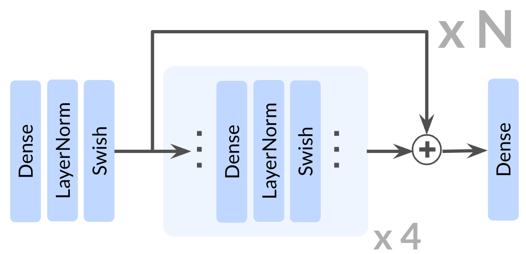
The study used contrastive reinforcement learning (CRL), a self-supervised method where agents learn to reach goals through exploration alone. Networks were scaled from the standard 4 layers up to 1024 layers—over 100 times deeper than typical RL architectures. To stabilize training at these depths, the team incorporated residual connections, layer normalization, and Swish activation functions. Experiments spanned ten tasks including locomotion (humanoid and ant agents), navigation through mazes, and robotic arm manipulation. Training used GPU-accelerated environments to generate sufficient data for deep networks.

Key Findings

Increasing network depth produced dramatic performance improvements:

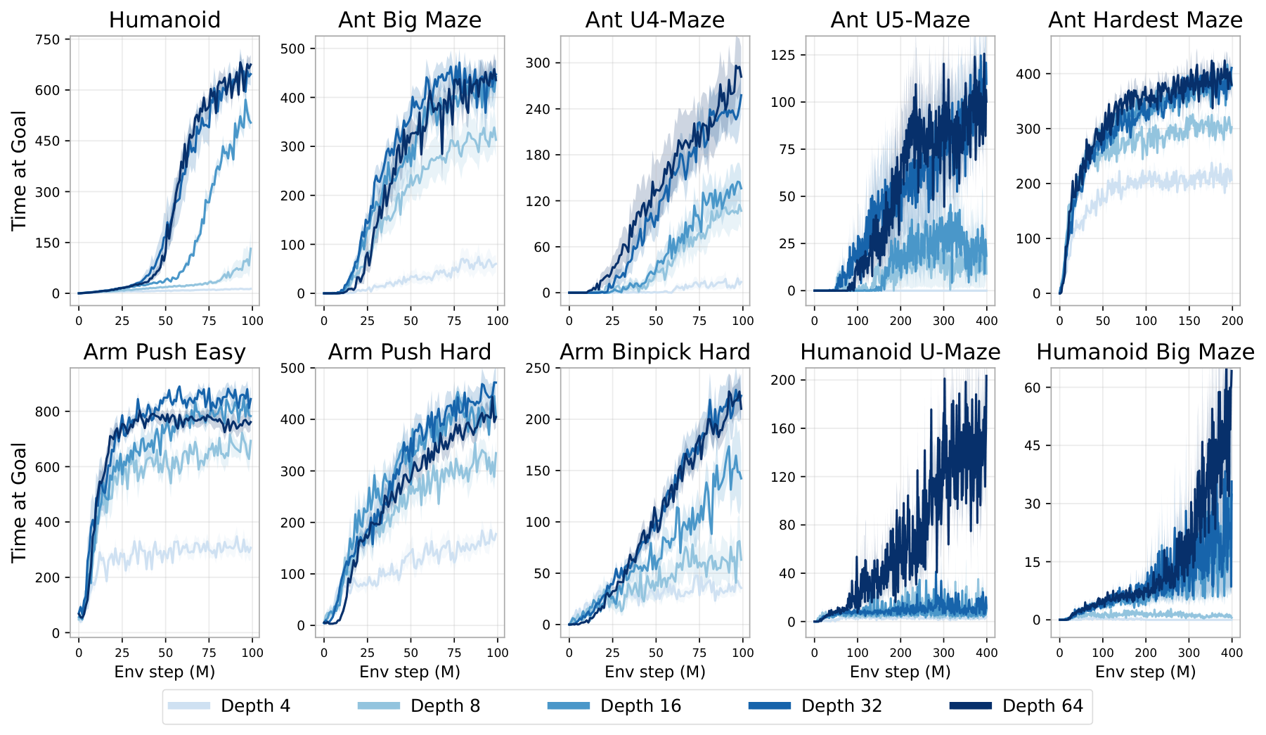
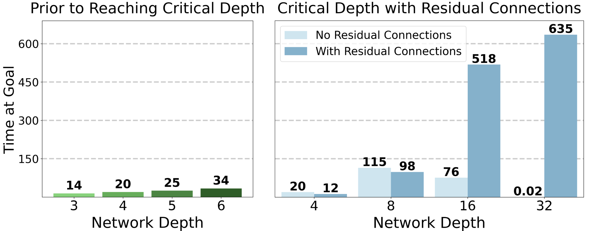
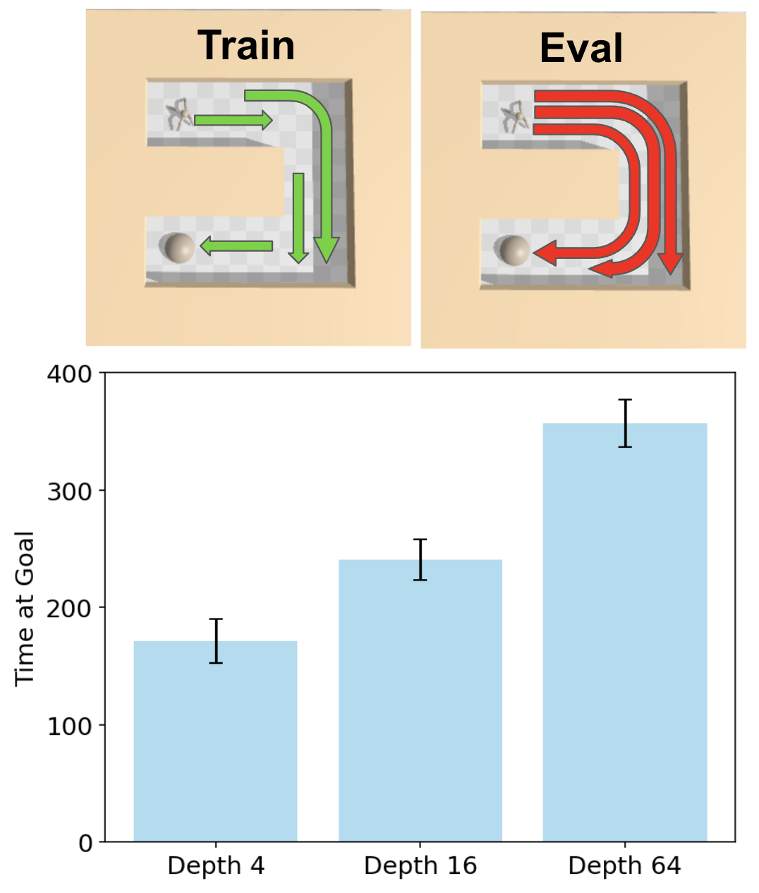
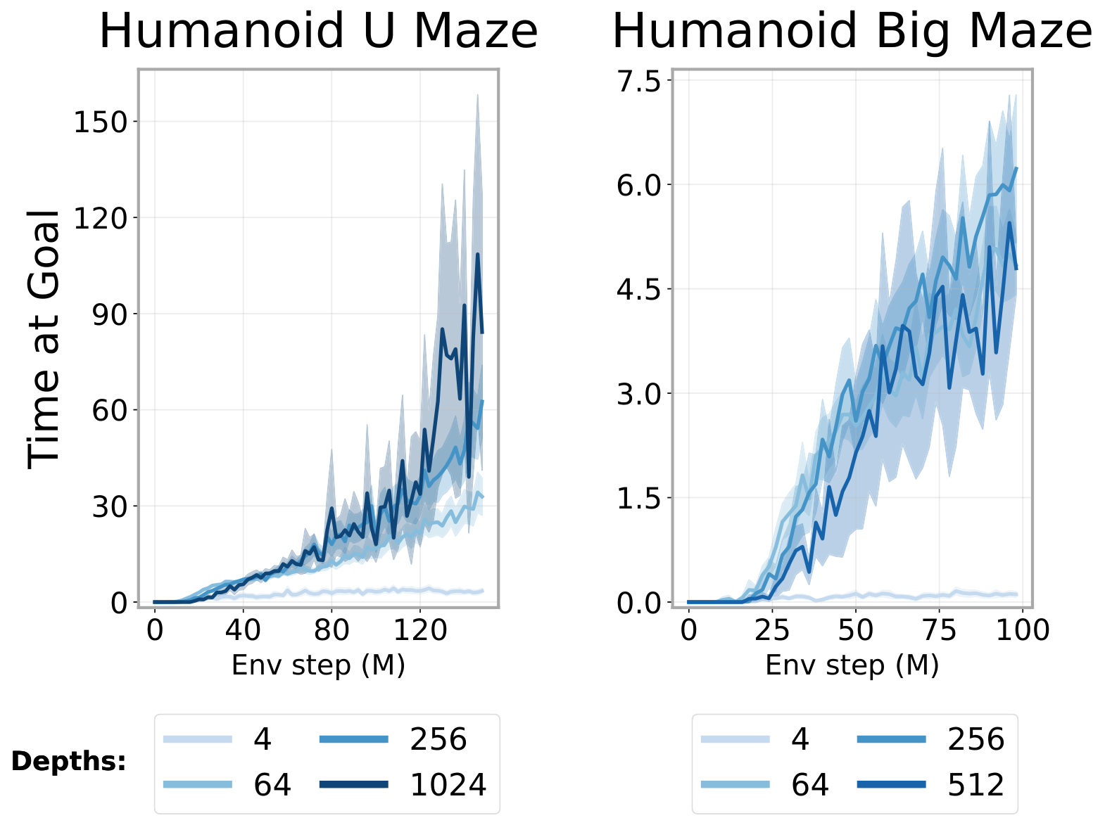
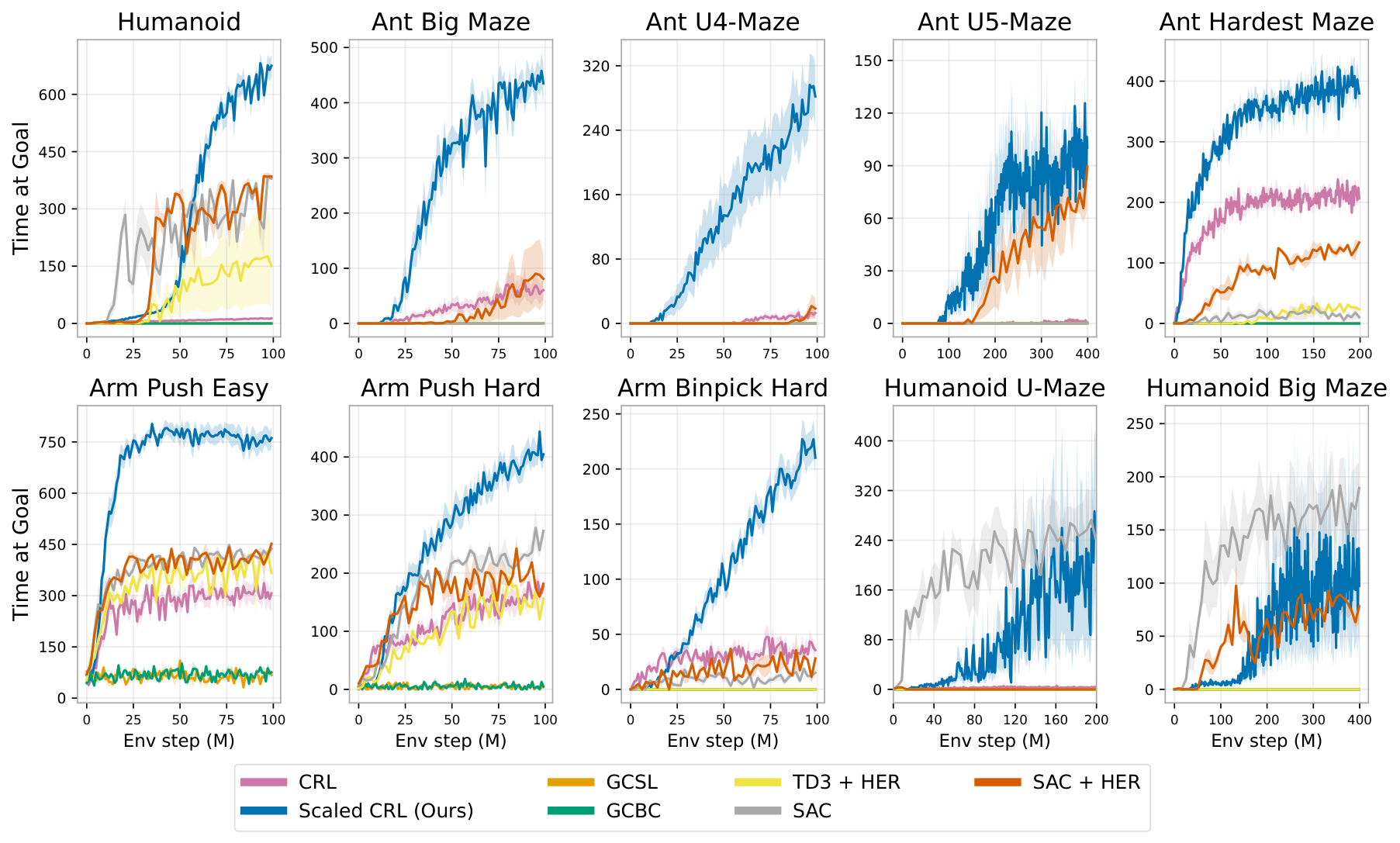
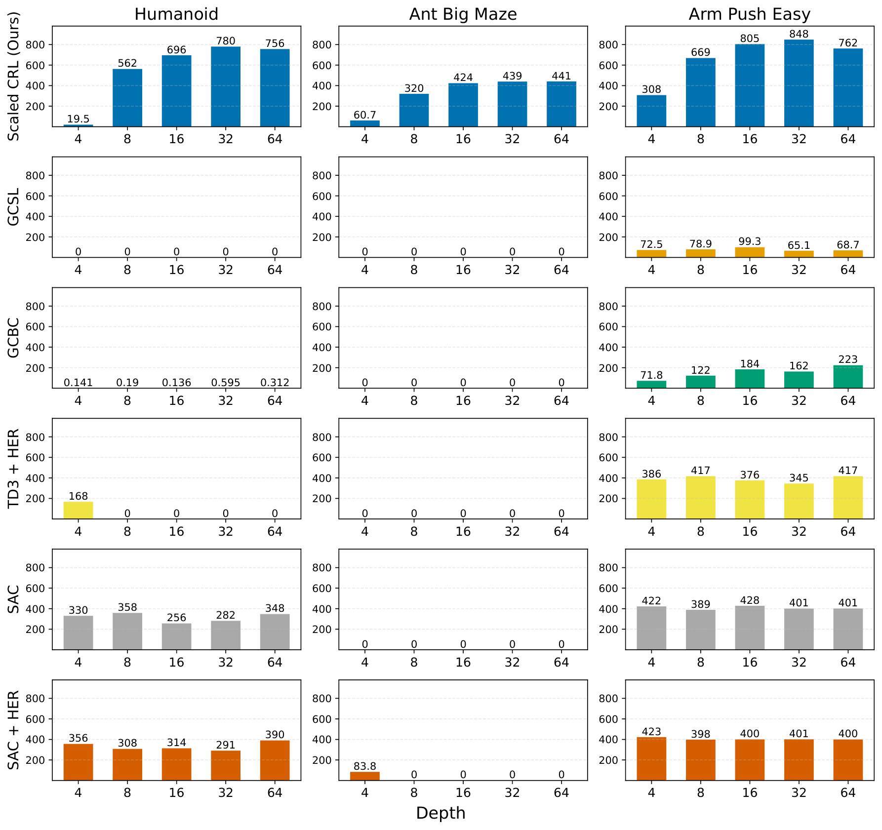
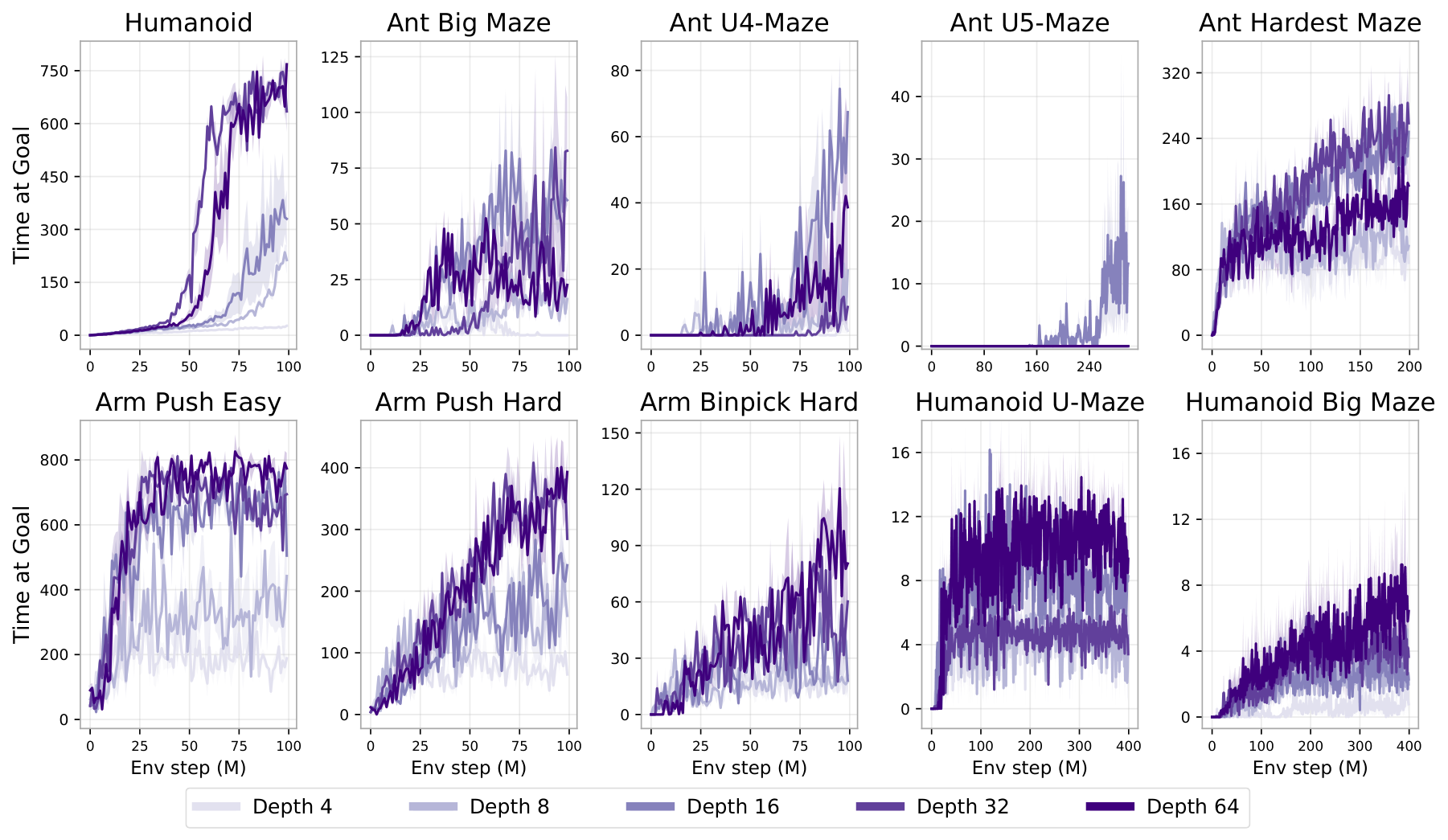
- Performance gains ranged from 2× to over 50× compared to standard 4-layer networks, depending on the task - The deepest humanoid tasks benefited most, with 50× improvements and qualitatively new behaviors emerging at specific depth thresholds - Performance often jumped discontinuously at critical depths rather than improving smoothly (for example, at 8 layers for Ant Big Maze, 64 layers for Humanoid U-Maze) - The scaled approach outperformed all standard goal-reaching baselines in 8 of 10 environments

Depth scaling proved more effective than width scaling. Simply doubling the network depth from 4 to 8 layers (holding width constant) outperformed networks made much wider while keeping depth at 4. Depth scaling also required fewer parameters for the same performance.

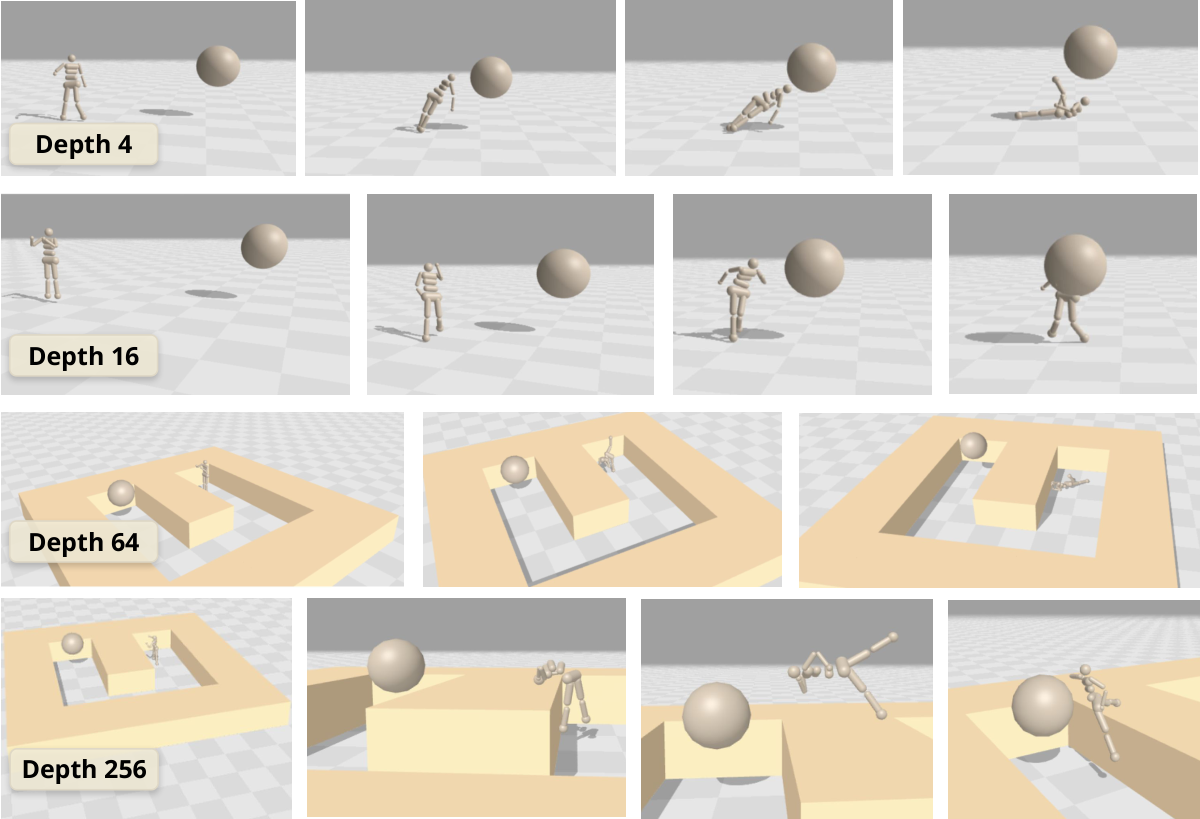
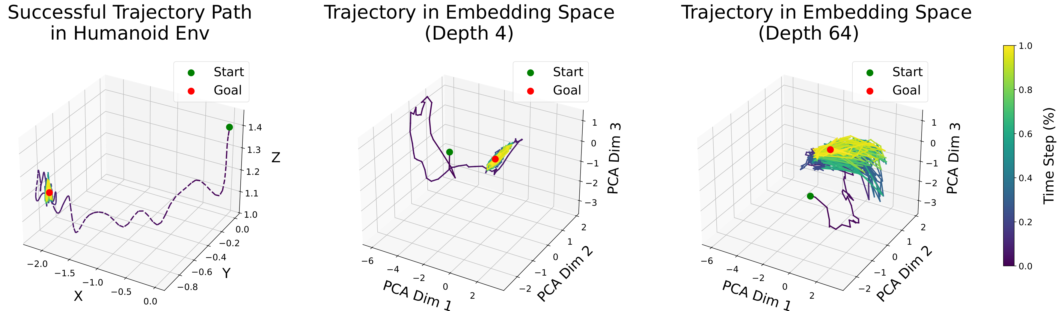
New capabilities emerged at greater depths. In humanoid tasks, 4-layer networks produced crude behaviors like falling toward the goal. At 16 layers, agents learned to walk upright. At 256 layers, agents developed acrobatic maneuvers including vaulting over walls and worming through obstacles—behaviors never before documented in goal-conditioned RL.

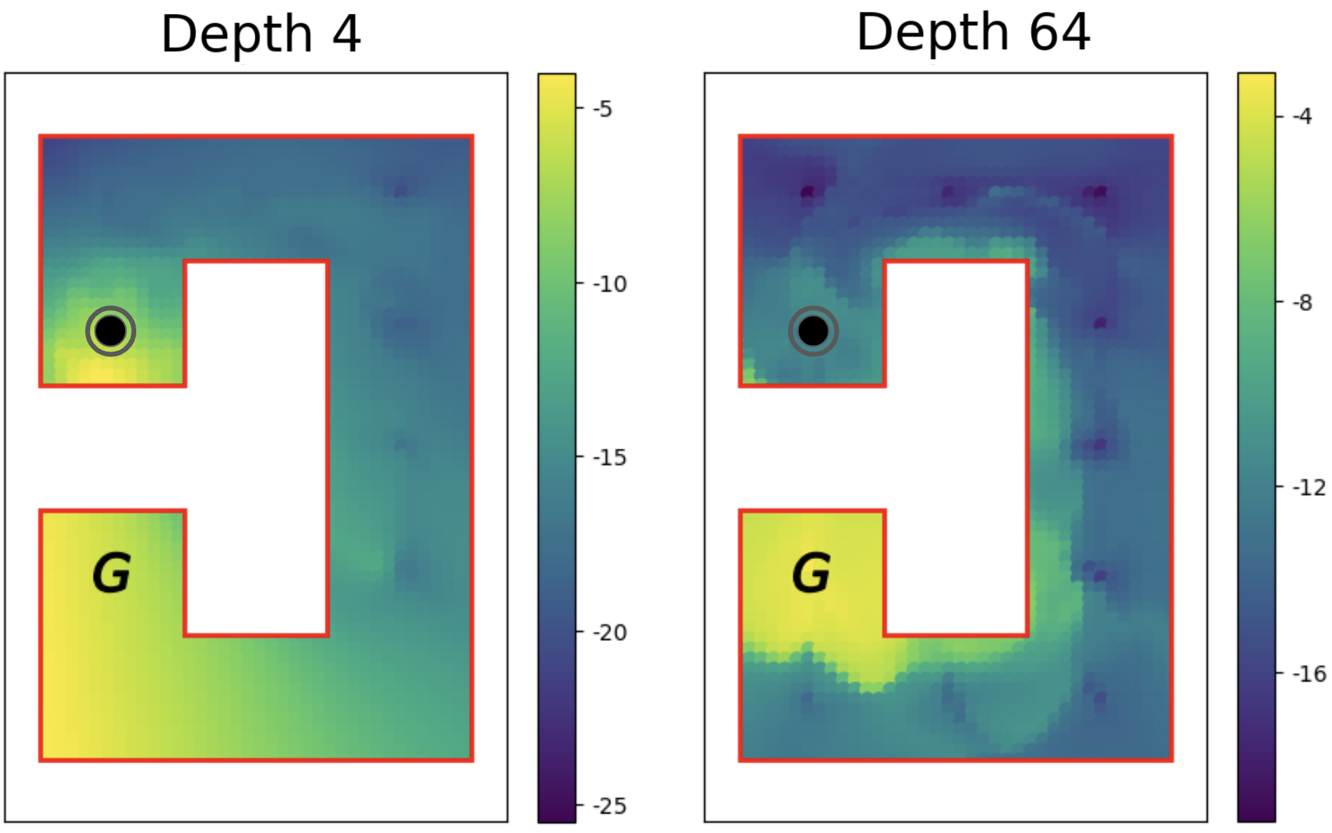
Deeper networks learned richer representations of the environment. Analysis showed that deep networks allocated more representational capacity to critical state regions and better captured environment topology, enabling them to navigate complex mazes where shallow networks failed.

What This Means

These results challenge the conventional wisdom that RL cannot benefit from depth scaling like other domains. The work demonstrates that with the right algorithmic and architectural choices—specifically self-supervised learning combined with residual networks—RL can achieve the kind of scaling benefits seen in language and vision.

The emergence of qualitatively new behaviors at specific depth thresholds mirrors "emergent capabilities" observed in large language models, suggesting RL may follow similar scaling laws. This has implications for cost-performance tradeoffs: depth scaling is parameter-efficient, so achieving better performance through depth rather than width reduces memory requirements and potentially computational costs.

However, the benefits come with increased training time. Wall-clock time scales approximately linearly with depth beyond a certain point. For the deepest networks (1024 layers), training required over 130 hours compared to 3 hours for 4-layer networks.

Limitations and Confidence

The scaling benefits did not transfer to offline settings where the agent learns from a fixed dataset rather than active exploration. Preliminary experiments with offline goal-conditioned RL showed no improvement or degradation with increased depth, indicating the approach is specific to online learning scenarios.

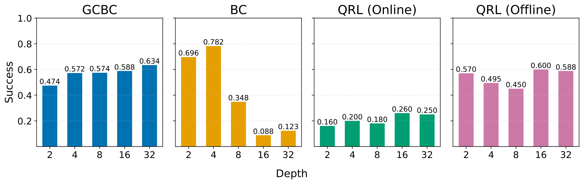
The study focused on one self-supervised algorithm (CRL). While experiments with other algorithms showed mixed results—no benefit for temporal difference methods, some benefit for behavioral cloning on simple tasks—the generality of depth scaling across RL methods remains unclear.

Results are based on simulated environments. Real-world robotic applications may face additional challenges not captured in simulation, and the computational costs may be prohibitive for resource-constrained deployments.

Recommendations and Next Steps

Organizations working on goal-reaching RL should consider depth as the primary scaling axis rather than width, particularly for complex tasks with high-dimensional observations. For tasks where small networks already achieve some success, depth scaling may yield marginal benefits; focus scaling efforts on the most challenging problems where standard approaches fail.

Before deploying in production, conduct pilot studies to verify that scaling benefits transfer to your specific domain and task complexity. Monitor wall-clock training time carefully, as computational costs increase substantially with depth.

For research teams, priority next steps include: investigating distributed training approaches to manage computational costs at scale; testing whether techniques like pruning and distillation can reduce inference costs while preserving deep network benefits; and determining which other self-supervised RL algorithms can benefit from depth scaling. Understanding why depth scaling fails in offline settings is critical for broader applicability.

The work provides building blocks for scalable RL but should be viewed as an early step. Achieving the full potential of scaling in RL will likely require discovering additional components beyond those identified here.

Kevin Wang
Princeton University
[email protected]

Ishaan Javali
Princeton University
[email protected]

Michał Bortkiewicz
Warsaw University of Technology
[email protected]

Tomasz Trzciński
Warsaw University of Technology,
Tooploox, IDEAS Research Institute

Benjamin Eysenbach
Princeton University
[email protected]

Abstract

Scaling up self-supervised learning has driven breakthroughs in language and vision, yet comparable progress has remained elusive in reinforcement learning (RL). In this paper, we study building blocks for self-supervised RL that unlock substantial improvements in scalability, with network depth serving as a critical factor. Whereas most RL papers in recent years have relied on shallow architectures (around 2 – 5 layers), we demonstrate that increasing the depth up to 1024 layers can significantly boost performance. Our experiments are conducted in an unsupervised goal-conditioned setting, where no demonstrations or rewards are provided, so an agent must explore (from scratch) and learn how to maximize the likelihood of reaching commanded goals. Evaluated on simulated locomotion and manipulation tasks, our approach increases performance on the self-supervised contrastive RL algorithm by

2×2\times

–

50×50\times

, outperforming other goal-conditioned baselines. Increasing the model depth not only increases success rates but also qualitatively changes the behaviors learned. The project webpage and code can be found here: https://wang-kevin3290.github.io/scaling-crl/.

1. Introduction

Show me a brief summary.

In this section, the authors address why scaling model size in reinforcement learning has not achieved the transformative breakthroughs seen in language and vision domains, where deep networks with hundreds of layers are commonplace while typical RL models use only 2-5 layers. They argue that the conventional wisdom of using RL merely for finetuning large self-supervised models misses the potential of self-supervised RL methods that can explore and learn without rewards or demonstrations. The authors propose integrating self-supervised RL—specifically contrastive RL—with GPU-accelerated frameworks, architectural techniques like residual connections and layer normalization, and dramatically increased network depth up to 1024 layers. This combination of building blocks enables RL to scale effectively along the depth dimension, achieving performance improvements of 2× to 50× across locomotion and manipulation tasks, with critical depth thresholds triggering the emergence of qualitatively distinct, previously unseen behaviors.

While scaling model size has been an effective recipe in many areas of machine learning, its role and impact in reinforcement learning (RL) remains unclear. The typical model size for state-based RL tasks is between 2 to 5 layers ([1, 2]). In contrast, it is not uncommon to use very deep networks in other domain areas; Llama 3 ([3]) and Stable Diffusion 3 ([4]) have hundreds of layers. In fields such as vision ([5, 6, 7]) and language ([8]), models often only acquire the ability to solve certain tasks once the model is larger than a critical scale. In the RL setting, many researchers have searched for similar emergent phenomena ([8]), but these papers typically report only small marginal benefits and typically only on tasks where small models already achieve some degree of success ([9, 10, 11]). A key open question in RL today is whether it is possible to achieve similar jumps in performance by scaling RL networks.

At first glance, it makes sense why training very large RL networks should be difficult: the RL problem provides very few bits of feedback (e.g., only a sparse reward after a long sequence of observations), so the ratio of feedback to parameters is very small. The conventional wisdom ([12]), reflected in many recent models ([13, 14, 15]), has been that large AI systems must be trained primarily in a self-supervised fashion and that RL should only be used to finetune these models. Indeed, many of the recent breakthroughs in other fields have been primarily achieved with self-supervised methods, whether in computer vision ([16, 5, 17]), NLP ([8]) or multimodal learning ([18]). Thus, if we hope to scale reinforcement learning methods, self-supervision will likely be a key ingredient.

In this paper, we will study building blocks for scaling reinforcement learning. Our first step is to rethink the conventional wisdom above: "reinforcement learning" and "self-supervised learning" are not diametric learning rules, but rather can be married together into self-supervised RL systems that explore and learn policies without reference to a reward function or demonstrations ([19, 20, 21]). In this work, we use one of the simplest self-supervised RL algorithms, contrastive RL (CRL) ([20]). The second step is to recognize the importance of increasing available data. We will do this by building on recent GPU-accelerated RL frameworks ([22, 23, 24, 25]). The third step is to increase network depth, using networks that are up to

100×100\times

deeper than those typical in prior work. Stabilizing the training of such networks will require incorporating architectural techniques from prior work, including residual connections ([26]), layer normalization ([27]), and Swish activation ([28]). Our experiments will also study the relative importance of batch size and network width.

The primary contribution of this work is to show that a method that integrates these building blocks into a single RL approach exhibits strong scalability:

Empirical Scalability: We observe a significant performance increase, more than $20×20\times$ in half of the environments and out-performing other standard goal-conditioned baselines. These performances gains correspond to qualitatively distinct policies that emerge with scale.
Scaling Depth in Network Architecture: While many prior RL works have primarily focused on increasing network width, they often report limited or even negative returns when expanding depth ([10, 9]). In contrast, our approach unlocks the ability to scale along the axis of depth, yielding performance improvements that surpass those from scaling width alone (see Section 4).
Empirical Analysis: We conduct an extensive analysis of the key components in our scaling approach, uncovering critical factors and offering new insights.

We anticipate that future research may build on this foundation by uncovering additional building blocks.

2. Related Work

Show me a brief summary.

In this section, the authors contextualize their work within the broader challenge of scaling reinforcement learning, noting that while NLP and computer vision have achieved transformative breakthroughs through self-supervised learning and deep architectures, RL has lagged behind due to obstacles like parameter underutilization, plasticity loss, data sparsity, and training instabilities. Most existing scaling efforts in RL remain confined to specific domains such as imitation learning or discrete action spaces, with recent work primarily focusing on increasing network width rather than depth, typically employing only four MLP layers and reporting limited gains from additional depth. The authors position their approach as distinct by successfully scaling network depth up to 1024 layers, leveraging contrastive RL's InfoNCE objective—a generalization of cross-entropy loss that frames RL as classifying trajectory membership. This classification-based formulation, echoing successful scaling principles in NLP, emerges as a potential fundamental building block for scalable reinforcement learning.

Natural Language Processing (NLP) and Computer Vision (CV) have recently converged in adopting similar architectures (i.e. transformers) and shared learning paradigms (i.e self-supervised learning), which together have enabled transformative capabilities of large-scale models ([29, 8, 6, 7, 30]). In contrast, achieving similar advancements in reinforcement learning (RL) remains challenging. Several studies have explored the obstacles to scaling large RL models, including parameter underutilization ([31]), plasticity and capacity loss ([32, 33]), data sparsity ([34, 12]), and training instabilities ([35, 36, 37, 38]). As a result, current efforts to scale RL models are largely restricted to specific problem domains, such as imitation learning ([39]), multi-agent games ([40]), language-guided RL ([41, 42]), and discrete action spaces ([31, 43]).

Recent approaches suggest several promising directions, including new architectural paradigms ([31]), distributed training approaches ([35, 44]), distributional RL ([45]), and distillation ([46]). Compared to these approaches, our method makes a simple extension to an existing self-supervised RL algorithm. The most recent works in this vein include [10] and [9], which leverage residual connections to facilitate the training of wider networks. These efforts primarily focus on network width, noting limited gains from additional depth, thus both works use architectures with only four MLP layers. In our method, we find that scaling width indeed improves performance (Section 4.4); however, our approach also enables scaling along depth, proving to be more powerful than width alone.

One notable effort to train deeper networks is described by [11], who cast value-based RL into a classification problem by discretizing the TD objective into a categorical cross-entropy loss. This approach draws on the conjecture that classification-based methods can be more robust and stable and thus may exhibit better scaling properties than their regressive counterparts ([47, 11]). The CRL algorithm that we use effectively uses a cross-entropy loss as well ([20]). Its InfoNCE objective is a generalization of the cross-entropy loss, thereby performing RL tasks by effectively classifying whether current states and actions belong to the same or different trajectory that leads toward a goal state. In this vein, our work serves as a second piece of evidence that classification, much like cross-entropy's role in the scaling success in NLP, could be a potential building block in RL.

3. Preliminaries

Show me a brief summary.

In this section, the mathematical foundation for goal-conditioned reinforcement learning and contrastive RL is established to frame the scaling experiments. A goal-conditioned MDP extends standard RL by having agents learn to reach arbitrary commanded goals, where the reward function reflects the probability of reaching a specified goal state in the next timestep. The contrastive RL algorithm solves this problem through an actor-critic framework, using an InfoNCE objective to train a critic that learns embeddings distinguishing same-trajectory state-action-goal tuples from random negatives, effectively casting the RL problem as classification. The policy is then trained to maximize this critic's output. Residual connections are incorporated into the architecture to enable gradient flow through deep networks by adding learned residual transformations to input representations rather than learning entirely new mappings, creating shortcut paths that preserve useful features from earlier layers and stabilize training of the 1000-layer networks central to this work.

This section introduces notation and definitions for goal-conditioned RL and contrastive RL. Our focus is on online RL, where a replay buffer stores the most recent trajectories, and the critic is trained in a self-supervised manner.

Goal-Conditioned Reinforcement Learning

We define a goal-conditioned MDP as tuple

Mg=(S,A,p0,p,pg,rg,γ)\mathcal{M}_g = (\mathcal{S}, \mathcal{A}, p_0, p, p_g, r_g, \gamma)

, where the agent interacts with the environment to reach arbitrary goals ([48, 34, 49]). At every time step

t

, the agent observes state

st∈Ss_t \in \mathcal{S}

and performs a corresponding action

at∈Aa_t \in \mathcal{A}

. The agent starts interaction in states sampled from

p_0(s_0)

, and the interaction dynamics are defined by the transition probability distribution

p(st+1∣st,at)p(s_{t+1} \mid s_{t}, a_{t})

. Goals

\in \mathcal{G}

are defined in a goal space

G\mathcal{G}

, which is related to

S\mathcal{S}

via a mapping

\mathcal{S} \to \mathcal{G}

. For example,

G\mathcal{G}

may correspond to a subset of state dimensions. The prior distribution over goals is defined by

p_g(g)

. The reward function is defined as the probability density of reaching the goal in the next time step

rg(st,at)≜(1−γ)p(st+1=g∣st,at)r_g(s_{t}, a_{t}) \triangleq (1-\gamma)p(s_{t+1} = g \mid s_t, a_t)

, with discount factor

γ\gamma

In this setting, the goal-conditioned policy

π(a∣s,g)\pi(a \mid s, g)

receives both the current observation of the environment as well as a goal. We define the discounted state visitation distribution as

pγπ(⋅∣⋅,g)(s)≜(1−γ)∑t=0∞γtptπ(⋅∣⋅,g)(s)p^{\pi\left(\cdot \mid \cdot, g\right)}_{\gamma}(s) \triangleq (1-\gamma)\sum_{t=0}^{\infty} \gamma^{t} p^{\pi\left(\cdot \mid \cdot, g\right)}_{t}(s)

, where

ptπ(s)p_t^\pi(s)

is the probability that policy

π\pi

visits

s

after exactly

t

steps, when conditioned with

g

. This last expression is precisely the

Q

-function of the policy

π(⋅∣⋅,g)\pi(\cdot \mid \cdot, g)

for the reward

r_{g}

Qgπ(s,a)≜pγπ(⋅∣⋅,g)(g∣s,a)Q^{\pi}_{g}(s, a) \triangleq p^{\pi\left(\cdot \mid \cdot, g\right)}_{\gamma}(g \mid s, a)

. The objective is to maximize the expected reward:

Contrastive Reinforcement Learning.

Our experiments will use the contrastive RL algorithm ([20]) to solve goal-conditioned problems. Contrastive RL is an actor-critic method; we will use

fϕ,ψ(s,a,g)f_{\phi, \psi}(s, a, g)

to denote the critic and

πθ(a∣s,g)\pi_{\theta}(a \mid s, g)

to denote the policy. The critic is parametrized with two neural networks that return state, action pair embedding

ϕ(s,a)\phi(s, a)

and goal embedding

ψ(g)\psi(g)

. The critic's output is defined as the

l^2

-norm between these embeddings:

fϕ,ψ(s,a,g)=∥ϕ(s,a)−ψ(g)∥2f_{\phi, \psi}(s, a, g) = \|\phi(s, a) - \psi(g)\|_2

. The critic is trained with the InfoNCE objective ([50]) as in previous works ([20, 19, 51, 52, 53, 25]). Training is conducted on batches

B\mathcal{B}

, where

s_i, a_i, g_i

represent the state, action, and goal (future state) sampled from the same trajectory, while

g_j

represents a goal sampled from a different, random trajectory. The objective function is defined as:

The policy

πθ(a∣s,g)\pi_\theta(a \mid s, g)

is trained to maximize the critic:

Residual Connections

We incorporate residual connections ([26]) into our architecture, following their successful use in RL ([11, 10, 9]). A residual block transforms a given representation

hi\mathbf{h}_i

by adding a learned residual function

Fi(hi)F_i(\mathbf{h}_i)

to the original representation. Mathematically, this is expressed as:

where

hi+1\mathbf{h}_{i+1}

is the output representation,

hi\mathbf{h}_i

is the input representation, and

Fi(hi)F_i(\mathbf{h}_i)

is a transformation learned through the network (e.g., using one or more layers). The addition ensures that the network learns modifications to the input rather than entirely new transformations, helping to preserve useful features from earlier layers. Residual connections improve gradient propagation by introducing shortcut paths ([54, 55]), enabling more effective training of deep models.

4. Experiments

Show me a brief summary.

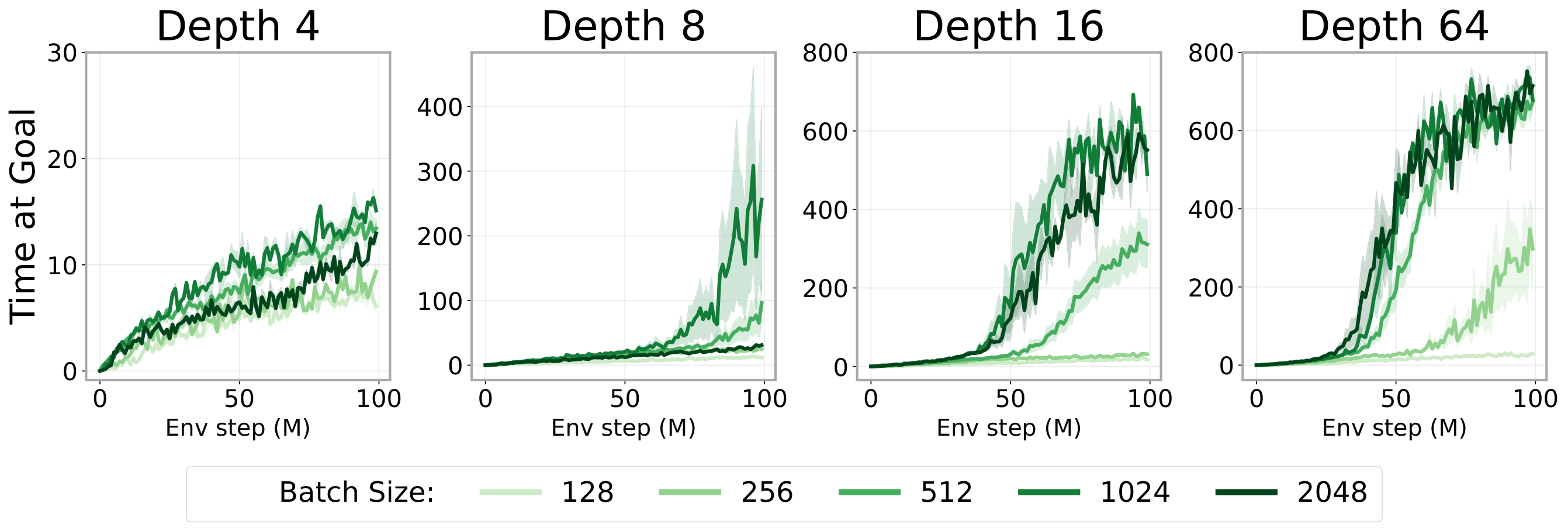
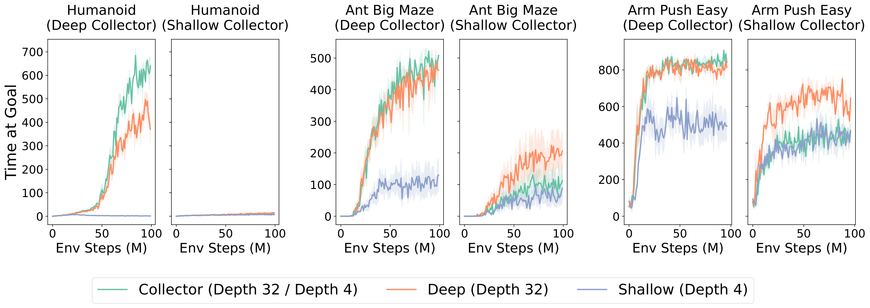
In this section, the authors investigate whether scaling network depth can unlock substantial performance gains in self-supervised reinforcement learning using contrastive RL (CRL). They demonstrate that increasing depth from the typical 4 layers to 64, 256, or even 1024 layers yields 2× to 50× performance improvements across locomotion, navigation, and manipulation tasks, with performance jumps occurring at critical depth thresholds that correspond to qualitatively distinct emergent behaviors. Depth scaling proves more effective than width scaling, particularly as observation dimensionality increases, and enables the network to leverage larger batch sizes. The improvements arise from a synergistic combination of enhanced exploration and greater representational capacity: deeper networks learn richer contrastive representations that capture environment topology, allocate more capacity to goal-relevant states, and exhibit partial experience stitching for generalization. However, these benefits depend critically on the CRL algorithm itself, as traditional TD methods and offline settings show minimal gains from depth scaling.

4.1 Experimental Setup

Environments.

All RL experiments use the JaxGCRL codebase ([25]), which facilitates fast online GCRL experiments based on Brax ([56]) and MJX ([57]) environments. The specific environments used are a range of locomotion, navigation, and robotic manipulation tasks, for details see Appendix B. We use a sparse reward setting, with

r = 1

only when the agent is in the goal proximity. For evaluation, we measure the number of time steps (out of 1000) that the agent is near the goal. When reporting an algorithm's performance as a single number, we compute the average score over the last five epochs of training.

Architectural Components

We employ residual connections from the ResNet architecture ([26]), with each residual block consisting of four repeated units of a Dense layer, a Layer Normalization ([27]) layer, and Swish activation ([28]). We apply the residual connections immediately following the final activation of the residual block, as shown in Figure 2. In this paper, we define the depth of the network as the total number of Dense layers across all residual blocks in the architecture. In all experiments, the depth refers to the configuration of the actor network and both critic encoder networks, which are scaled jointly, except for the ablation experiment in Section 4.4.

4.2 Scaling Depth in Contrastive RL

We start by studying how increasing network depth can increase performance. Both the JaxGCRL benchmark and relevant prior work ([10, 9, 52]) use MLPs with a depth of 4, and as such we adopt it as our baseline. In contrast, we will study networks of depth 8, 16, 32, and 64. The results in Figure 1 demonstrate that deeper networks achieve significant performance improvements across a diverse range of locomotion, navigation, and manipulation tasks. Compared to the 4-layer models typical in prior work, deeper networks achieve

\times

gains in robotic manipulation tasks, over

20×20\times

gains in long-horizon maze tasks such as Ant U4-Maze and Ant U5-Maze, and over

50×50\times

gains in humanoid-based tasks. The full table of performance increases up to depth 64 is provided in Table 1.

In Figure 13, we present results the same 10 environments, but compared against SAC, SAC+HER, TD3+HER, GCBC, and GCSL. Scaling CRL leads to substantial performance improvements, outperforming all other baselines in 8 out of 10 tasks. The only exception is SAC on the Humanoid Maze environments, where it exhibits greater sample efficiency early on; however, scaled CRL eventually reaches comparable performance. These results highlight that scaling the depth of the CRL algorithm enables state-of-the-art performance in goal-conditioned reinforcement learning.

4.3 Emergent Policies Through Depth

A closer examination of the results from the performance curves in Figure 1 reveals a notable pattern: instead of a gradual improvement in performance as depth increases, there are pronounced jumps that occur once a critical depth threshold is reached (also shown in Figure 5). The critical depths vary by environment, ranging from 8 layers (e.g. Ant Big Maze) to 64 layers in the Humanoid U-Maze task, with further jumps occurring even at depths of 1024 layers (see the Testing Limits section, Section 4.4).

Prompted by this observation, we visualized the learned policies at various depths and found qualitatively distinct skills and behaviors exhibited. This is particularly pronounced in the humanoid-based tasks, as illustrated in Figure 3. Networks with a depth of 4 exhibit rudimentary policies where the agent either falls or throws itself toward the target. Only at a critical depth of 16 does the agent develop the ability to walk upright into the goal. In the Humanoid U-Maze environment, networks of depth 64 struggle to navigate around the intermediary wall, collapsing on the ground. Remarkably at a depth of 256, the agent learns unique behaviors on Humanoid U-Maze. These behaviors include folding forward into a leveraged position to propel itself over walls and shifting into a seated posture over the intermediary obstacle to worm its way toward the goal (one of these policies is illustrated in the fourth row of Figure 3). To the best of our knowledge, this is the first goal-conditioned approach to document such behaviors on the humanoid environment.

4.4 What Matters for CRL Scaling

Width vs. Depth

Figure 4: Scaling network width vs. depth. Here, we reflect findings from previous works ([10, 9]) which suggest that increasing network width can enhance performance. However, in contrast to prior work, our method is able to scale depth, yielding more impactful performance gains. For instance, in the Humanoid environment, raising the width to 2048 (depth=4) fails to match the performance achieved by simply doubling the depth to 8 (width=256). The comparative advantage of scaling depth is more pronounced as the observational dimensionality increases.

💭 Click to ask about this figure

Past literature has shown that scaling network width can be effective ([10, 9]). In Figure 4, we find that scaling width is also helpful in our experiments: wider networks consistently outperform narrower networks (depth held constant at 4). However, depth seems to be a more effective axis for scaling: simply doubling the depth to 8 (width held constant at 256) outperforms the widest networks in all three environments. The advantage of depth scaling is most pronounced in the Humanoid environment (observation dimension 268), followed by Ant Big Maze (dimension 29) and Arm Push Easy (dimension 17), suggesting that the comparative benefit may increase with higher observation dimensionality.

Note additionally that the parameter count scales linearly with width but quadratically with depth. For comparison, a network with 4 MLP layers and 2048 hidden units has roughly 35M parameters, while one with a depth of 32 and 256 hidden units has only around 2M. Therefore, when operating under a fixed FLOP compute budget or specific memory constraints, depth scaling may be a more computationally efficient approach to improving network performance.

Scaling the Actor vs. Critic Networks

To investigate the role of scaling in the actor and critic networks, Figure 6 presents the final performance for various combinations of actor and critic depths across three environments. Prior work ([9, 10]) focuses on scaling the critic network, finding that scaling the actor degrades performance. In contrast, while we do find that scaling the critic is more impactful in two of the three environments (Humanoid, Arm Push Easy), our method benefits from scaling the actor network jointly, with one environment (Ant Big Maze) demonstrating actor scaling to be more impactful. Thus, our method suggests that scaling both the actor and critic networks can play a complementary role in enhancing performance.

Deep Networks Unlock Batch Size Scaling

Scaling batch size has been well-established in other areas of machine learning ([58, 59]). However, this approach has not translated as effectively to reinforcement learning (RL), and prior work has even reported negative impacts on value-based RL ([60]). Indeed, in our experiments, simply increasing the batch size for the original CRL networks yields only marginal differences in performance (Figure 7, top left).

At first glance, this might seem counterintuitive: since reinforcement learning typically involves fewer informational bits per piece of training data ([12]), one might expect higher variance in batch loss or gradients, suggesting the need for larger batch sizes to compensate. At the same time, this possibility hinges on whether the model in question can actually make use of a bigger batch size—in domains of ML where scaling has been successful, larger batch sizes usually bring the most benefit when coupled with sufficiently large models ([59, 58]). One hypothesis is that the small models traditionally used in RL may obscure the underlying benefits of larger batch size.

To test this hypothesis, we study the effect of increasing the batch size for networks of varying depths. As shown in Figure 7, scaling the batch size becomes effective as network depth grows. This finding offers evidence that by scaling network capacity, we may simultaneously unlock the benefits of larger batch size, potentially making it an important component in the broader pursuit of scaling self-supervised RL.

Training Contrastive RL with 1000+ Layers

We next study whether further increasing depth beyond 64 layers further improves performance. We use the Humanoid maze tasks as these are both the most challenging environments in the benchmark and also seem to benefit from the deepest scaling. The results, shown in Figure 12, indicate that performance continues to substantially improve as network depth reaches 256 and 1024 layers in the Humanoid U-Maze environment. While we were unable to scale beyond 1024 layers due to computational constraints, we expect to see continued improvements with even greater depths, especially on the most challenging tasks.

Figure 8: We disentangle the effects of exploration and expressivity on depth scaling by training three networks in parallel: a “collector, ” plus one deep and one shallow learner that train only from the collector’s shared replay buffer. In all three environments, when using a deep collector (i.e. good data coverage), the deep learner outperforms the shallow learner, indicating that expressivity is crucial when controlling for good exploration. With a shallow collector (poor exploration), even the deep learner cannot overcome the limitations of insufficient data coverage. As such, the benefits of depth scaling arise from a combination of improved exploration and increased expressivity working jointly.

💭 Click to ask about this figure

4.5 Why Scaling Happens

Depth Enhances Contrastive Representations

$**Figure 9:** **Deeper Q-functions are qualitatively different.** In the U4-Maze, the start and goal positions are indicated by the $\odot$ and $\textbf{G}$ symbols respectively, and the visualized Q values are computed via the $L_2$ distance in the learned representation space, i.e., $Q(s, a, g) = \|\phi(s, a) - \psi(g)\|_2$. The shallow depth 4 network *(left)* naively relies on Euclidean proximity, showing high Q values near the start despite a maze wall. In contrast, the depth 64 network *(right)* clusters high Q values at the goal, gradually tapering along the interior.$

Figure 9: Deeper Q-functions are qualitatively different. In the U4-Maze, the start and goal positions are indicated by the $\odot$ and $\textbf{G}$ symbols respectively, and the visualized Q values are computed via the $L_2$ distance in the learned representation space, i.e., $Q(s, a, g) = \|\phi(s, a) - \psi(g)\|_2$ . The shallow depth 4 network (left) naively relies on Euclidean proximity, showing high Q values near the start despite a maze wall. In contrast, the depth 64 network (right) clusters high Q values at the goal, gradually tapering along the interior.

💭 Click to ask about this figure

The long-horizon setting has been a long-standing challenge in RL particularly in unsupervised goal-conditioned settings where there is no auxiliary reward feedback ([61]). The family of U-Maze environments requires a global understanding of the maze layout for effective navigation. We consider a variant of the Ant U-Maze environment, the U4-maze, in which the agent must initially move in the direction opposite the goal to loop around and ultimately reach it. As shown in Figure 9, we observe a qualitative difference in the behavior of the shallow network (depth 4) compared to the deep network (depth 64). The visualized Q-values computed from the critic encoder representations reveal that the depth 4 network seemingly relies on Euclidean distance to the goal as a proxy for the Q value, even when a wall obstructs the direct path. In contrast, the depth 64 critic network learns richer representations, enabling it to effectively capture the topology of the maze as visualized by the trail of high Q values along the inner edge. These findings suggest that increasing network depth leads to richer learned representations, enabling deeper networks to better capture environment topology and achieve more comprehensive state-space coverage in a self-supervised manner.

Depth Enhances Exploration and Expressivity in a Synergized Way

Our earlier results suggested that deeper networks achieve greater state-action coverage. To better understand why scaling works, we sought to determine to whether improved data alone explains the benefits of scaling, or whether it acts in conjunction with other factors. Thus, we designed an experiment in Figure 8 in which we train three networks in parallel: one network, the “collector, " interacts with the environment and writes all experience to a shared replay buffer. Alongside it, two additional "learners", one deep and one shallow, train concurrently. Crucially, these two learners never collect their own data; they train only from the collector’s buffer. This design holds the data distribution constant while varying the model’s capacity, so any performance gap between the deep and shallow learners must come from expressivity rather than exploration. When the collector is deep (e.g., depth 32), across all three environments the deep learner substantially outperforms the shallow one across all three environments, indicating that the expressivity of the deep networks is critical. On the other hand, we repeat the experiment with shallow collectors (e.g., depth 4), which explores less effectively and therefore populates the buffer with low-coverage experience. Here, both the deep and shallow learners struggle and achieve similarly poor performance, which indicates that the deep network’s additional capacity does not overcome the limitations of insufficient data coverage. As such, scaling depth enhances exploration and expressivity in a synergized way: stronger learning capacity drives more extensive exploration, and strong data coverage is essential to fully realize the power of stronger learning capacity. Both aspects jointly contribute to improved performance.

💭 Click to ask about this figure

Deep Networks Learn to Allocate Greater Representational Capacity to States Near the Goal

In Figure 10 we take a successful trajectory in the Humanoid environment and visualize the embeddings of state-action encoder along this trajectory for both deep vs. shallow networks. While the shallow network (Depth 4) tends to cluster near-goal states tightly together, the deep network produces more "spread out" representations. This distinction is important: in a self-supervised setting, we want our representations to separate states that matter—particularly future or goal-relevant states—from random ones. As such, we want to allocate more representational capacity to such critical regions. This suggests that deep networks may learn to allocate representational capacity more effectively to state regions that matter most for the downstream task.

Deeper Networks Enable Partial Experience Stitching

Another key challenge in reinforcement learning is learning policies that can generalize to tasks unseen during training. To evaluate this setting, we designed a modified version of the Ant U-Maze environment. As shown in Figure 11 (top right), the original JaxGCRL benchmark assesses the agent's performance on the three farthest goal positions located on the opposite side of the wall. However, instead of training on all possible subgoals (a superset of the evaluation state-goal pairs), we modified the setup to train on start-goal pairs that are at most 3 units apart, ensuring that none of the evaluation pairs ever appear in the training set. Figure 11 demonstrates that depth 4 networks show limited generalization, solving only the easiest goal (4 units away from the start). Depth 16 networks achieve moderate success, while depth 64 networks excel, sometimes solving the most challenging goal position. These results suggest that the increasing network depth results in some degree of stitching, combining

≤\leq

3-unit pairs to navigate the 6-unit span of the U-Maze.

The (CRL) Algorithm is Key

In Appendix A, we show that scaled CRL outperforms other baseline goal-conditioned algorithms and advance the SOTA for goal-conditioned RL. We observe that for temporal difference methods (SAC, SAC+HER, TD3+HER), the performance saturates for networks of depth 4, and there is either zero or negative performance gains from deeper networks. This is in line with previous research showing that these methods benefit mainly from width ([10, 9]). These results suggest that the self-supervised CRL algorithm is critical.

We also experiment with scaling more self-supervised algorithms, namely Goal-Conditioned Behavioral Cloning (GCBC) and Goal-Conditioned Supervised Learning (GCSL). While these methods yield zero success in certain environments, they show some utility in arm manipulation tasks. Interestingly, even a very simple self-supervised algorithm like GCBC benefits from increased depth. This points to a promising direction for future work of further investigating other self-supervised methods to uncover potentially different or complementary recipes for scaling self-supervised RL.

Finally, recent work has augmented goal-conditioned RL with quasimetric architectures, leveraging the fact that temporal distances satisfy a triangle inequality–based invariance. In Appendix A, we also investigate whether the depth scaling effect persists when applied to these quasimetric networks.

💭 Click to ask about this figure

4.6 Does Depth Scaling Improve Offline Contrastive RL?

In preliminary experiments, we evaluated depth scaling in the offline goal-conditioned setting using OGBench ([62]). We found little evidence that increasing the network depth of CRL improves performance in this offline setting. To further investigate this, we conducted ablations: (1) scaling critic depth while holding the actor at 4 or 8 layers, and (2) applying cold initialization to the final layers of the critic encoders ([52]). In all cases, baseline depth 4 networks often had the highest success. A key direction for future work is to see if our method can be adapted to enable scaling in the offline setting.

5. Conclusion

Show me a brief summary.

In this section, the authors argue that emergent capabilities from scale have driven much of the success in vision and language models, yet a critical question remains: where does the data come from? Unlike supervised learning, reinforcement learning methods inherently address this by jointly optimizing both the model and the data collection process through exploration. Determining effective ways to build RL systems that demonstrate emergent capabilities may be important for transforming the field into one that trains its own large models. By integrating key components for scaling up RL into a single approach, the work shows that model performance consistently improves as scale increases in complex tasks. Additionally, deep models exhibit qualitatively better behaviors which might be interpreted as implicitly acquired skills necessary to reach the goal, suggesting that this work represents a step towards building RL systems with emergent capabilities at scale.

Show me a brief summary.

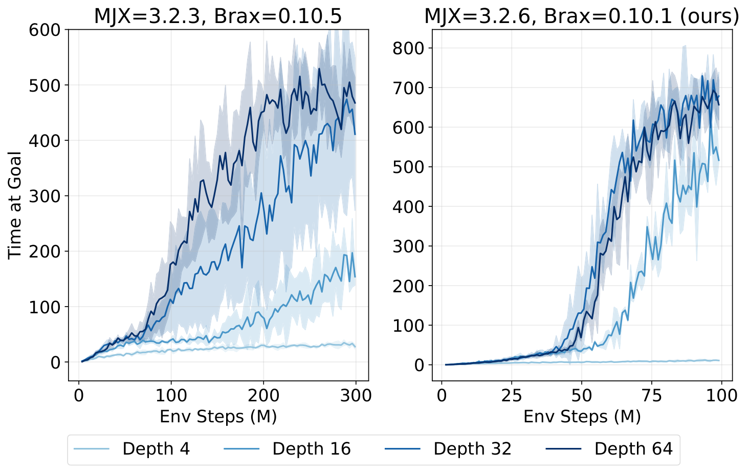
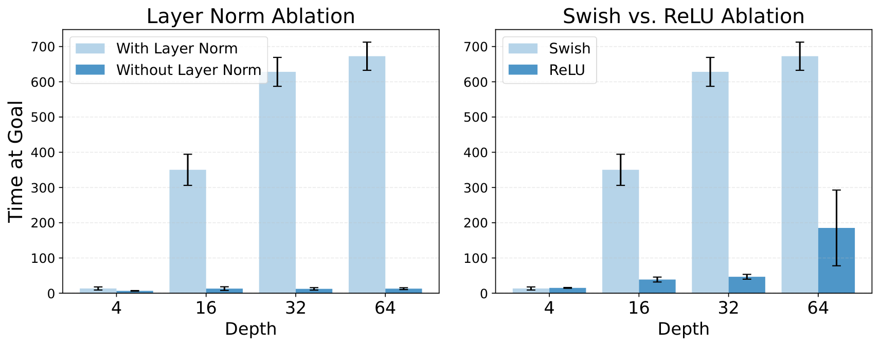
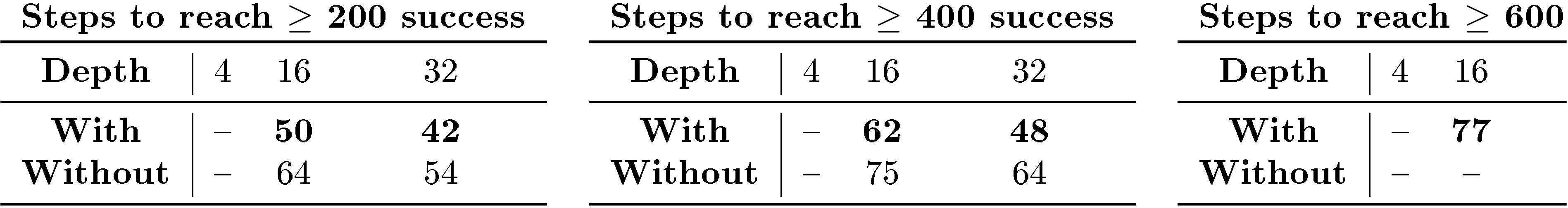
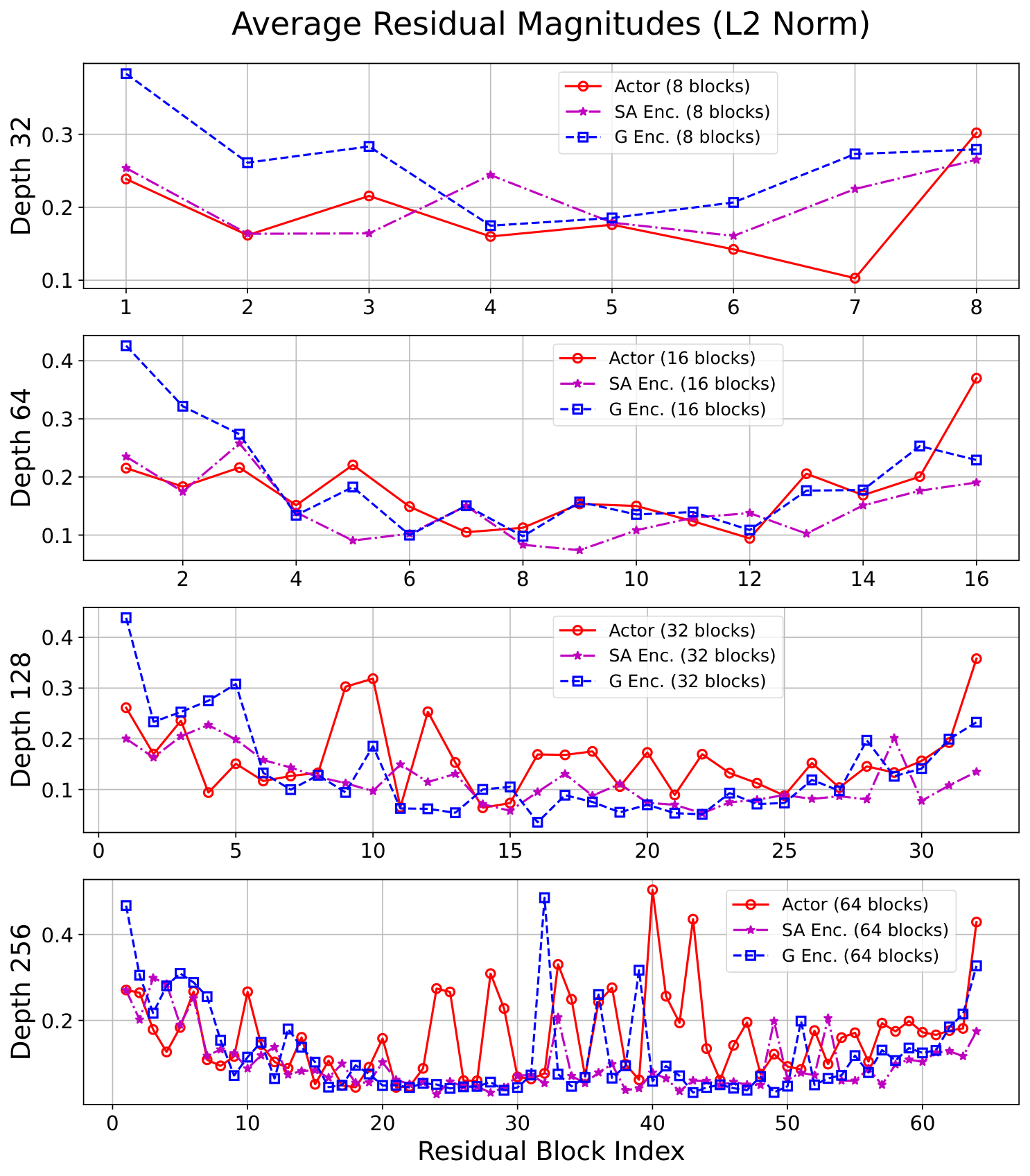
In this section, scaled contrastive reinforcement learning (CRL) demonstrates state-of-the-art performance in online goal-conditioned RL, outperforming baseline methods like SAC, TD3+HER, GCSL, and GCBC across eight of ten environments, while depth scaling proves ineffective for these baseline algorithms beyond four layers. Architectural components including residual connections, layer normalization, and Swish activations are essential for enabling depth scaling, with hyperspherical normalization further improving sample efficiency. The scaling benefits extend to quasimetric architectures and offline goal-conditioned behavioral cloning, though offline CRL scaling remains challenging. Residual activation norms decrease in deeper layers as expected, and wall-clock time increases approximately linearly with depth, yet the scaled approach often reaches superior performance faster than baselines. The experiments use the JaxGCRL benchmark with environments spanning locomotion, navigation, and manipulation tasks, demonstrating that combining self-supervised contrastive learning with deep residual architectures unlocks parameter scaling in reinforcement learning.

Arguably, much of the success of vision and language models today is due to the emergent capabilities they exhibit from scale ([8]), leading to many systems reducing the RL problem to a vision or language problem. A critical question for large AI models is: where does the data come from? Unlike supervised learning paradigms, RL methods inherently address this by jointly optimizing both the model and the data collection process through exploration. Ultimately, determining effective ways of building RL systems that demonstrate emergent capabilities may be important for transforming the field into one that trains its own large models. We believe that our work is a step towards these systems. By integrating key components for scaling up RL into a single approach, we show that model performance consistently improves as scale increases in complex tasks. In addition, deep models exhibit qualitatively better behaviors which might be interpreted as implicitly acquired skills necessary to reach the goal.

Limitations.

The primary limitations of our results are that scaling network depth comes at the cost of compute. An important direction for future work is to study how distributed training might be used to leverage even more compute, and how techniques such as pruning and distillation might be used to decrease the computational costs.

Impact Statement

This paper presents work whose goal is to advance the field of Machine Learning. There are many potential societal consequences of our work, none which we feel must be specifically highlighted here.

Acknowledgments.

We gratefully acknowledge Galen Collier, Director of Researcher Engagement, for support through the NSF grant, as well as the staff at Princeton Research Computing for their invaluable assistance. We also thank Colin Lu for his discussions and contributions to this work. This research was also partially supported by the National Science Centre, Poland (grant no. 2023/51/D/ST6/01609), and the Warsaw University of Technology through the Excellence Initiative: Research University (IDUB) program. Finally, we would also like to thank Jens Tuyls and Harshit Sikchi for providing helpful commends and feedback on the manuscript.

Appendix

A. Additional Experiments

A.1 Scaled CRL Outperforms All Other Baselines on 8 out of 10 Environments

In Figure 1, we demonstrated that increasing the depth of the CRL algorithm leads to significant performance improvements over the original CRL (see also Table 1). Here, we show that these gains translate to state-of-the-art results in online goal-conditioned RL, with Scaled CRL outperforming both standard TD-based methods such as SAC, SAC+HER, and TD3+HER, as well as self-supervised imitation-based approaches like GCBC and GCSL.

A.2 The CRL Algorithm is Key: Depth Scaling is Not Effective on Other Baselines

Next, we investigate whether increasing network depth in the baseline algorithms yields similar performance improvements as observed in CRL. We find that SAC, SAC+HER, and TD3+HER do not benefit from depths beyond four layers, which is consistent with prior findings ([10, 9]). Additionally, GCSL and GCBC fail to achieve any meaningful performance on the Humanoid and Ant Big Maze tasks. Interestingly, we do observe one exception, as GCBC exhibits improved performance with increased depth in the Arm Push Easy environment.

Table 1: Increasing network depth (depth $D = 4 \rightarrow 64$ ) increases performance on CRL (Figure 1). Scaling depth exhibits the greatest benefits on tasks with the largest observation dimension (Dim).

Task	Dim	$\textbf{D = }$ 4	$\textbf{D = }$ 64	Imprv.
Arm Binpick Hard	17	$38$ $\mathbf{\pm} 4$	$219$ $\mathbf{\pm} 15$	$5.7 \times$
Arm Push Easy		$308$ $\mathbf{\pm} 33$	$762$ $\mathbf{\pm} 30$	$2.5 \times$
Arm Push Hard		$171$ $\mathbf{\pm} 11$	$410$ $\mathbf{\pm} 13$	$2.4 \times$
Ant U4-Maze	29	$11.4$ $\mathbf{\pm } 4.1$	$286$ $\mathbf{\pm} 36$	$25 \times$

A.3 Additional Scaling Experiments: Offline GCBC, BC, and QRL

We further investigate several additional scaling experiments. As shown in Figure 15, our approach successfully scales with depth in the offline GCBC setting on the antmaze-medium-stitch task from OGBench. We find that our the combination of layer normalization, residual connections, and Swish activations is critical, suggesting that our architectural choices may be applied to unlock depth scaling in other algorithms and settings. We also attempt to scale depth for behavioral cloning and the QRL ([63]) algorithm—in both of these cases, however, we observe negative results.

A.4 Can Depth Scaling also be Effective for Quasimetric Architectures?

Prior work ([64, 65]) has found that temporal distances satisfy an important invariance property, suggesting the use of quasimetric architectures when learning temporal distances. Our next experiment tests whether changing the architecture affects the scaling properties of self-supervised RL. Specifically, we use the CMD-1 algorithm ([53]), which employs a backward NCE loss with MRN representations. The results indicate that scaling benefits are not limited to a single neural network parametrization. However, MRN’s poor performance on the Ant U5-Maze task suggests further innovation is needed for consistent scaling with quasimetric models.

A.5 Additional Architectural Ablations: Layer Norm and Swish Activation

We conduct ablation experiments to validate the architectural choices of layer norm and swish activation. Figure 17 shows that removing layer normalization performs significantly worse. Additionally, scaling with ReLU significantly hampers scalability. These results, along with Figure 5 show that all of our architectural components—residual connections, layer norm, and swish activations—are jointly essential to unlocking the full performance of depth scaling.

A.6 Can We Integrate Novel Architectural Innovations from the Emerging RL Scaling Literature?

Recently, Simba-v2 proposed a new architecture for scalable RL. Its key innovation is the replacement of layer normalization with hyperspherical normalization, which projects network weights onto the unit-norm hypersphere after each gradient update. As shown, the same depth-scaling trends hold when adding hyperspherical normalization to our architecture, and it further improves the sample efficiency of depth scaling. This demonstrates that our method can naturally incorporate new architectural innovations emerging in the RL scaling literature.

A.7 Residuals Norms in Deep Networks

Prior work has noted decreasing residual activation norms in deeper layers ([66]). We investigate whether this pattern also holds in our setting. For the critic, the trend is generally evident, especially in very deep architectures (e.g., depth 256). The effect is not as pronounced in the actor.

A.8 Scaling Depth for Offline Goal-conditioned RL

B. Experimental Details

B.1 Environment Setup and Hyperparameters

Our experiments use the JaxGCRL suite of GPU-accelerated environments, visualized in Figure 19, and a contrastive RL algorithm with hyperparameters reported in Table 7. In particular, we use 10 environments, namely:

ant_big_maze, ant_hardest_maze, arm_binpick_hard, arm_push_easy, arm_push_hard, humanoid, humanoid_big_maze, humanoid_u_maze, ant_u4_maze, ant_u5_maze

B.2 Python Environment Differences

In all plots presented in the paper, we used MJX 3.2.6 and Brax 0.10.1 to ensure a fair and consistent comparison. During development, we noticed discrepancies in physics behavior between the environment versions we employed (the CleanRL version of JaxGCRL) and the version recommended in a more recent commit of JaxGCRL ([25]). Upon examination, the performance differences (shown in Figure 20) stem from a difference in versions in the MJX and Brax packages. Nonetheless, in both sets of MJX and Brax versions, performance scales monotonically with depth.

B.3 Wall-clock Time of Our Approach

We report the wall-clock time of our approach in Table 3. The table shows results for depths of 4, 8, 16, 32, and 64 across all ten environments, and for the Humanoid U-Maze environment, scaling up to 1024 layers. Overall, wall-clock time increases approximately linearly with depth beyond a certain point.

Table 3: Wall-clock time (in hours) for Depth 4, 8, 16, 32, and 64 across all 10 environments.

Environment	Depth 4	Depth 8	Depth 16	Depth 32	Depth 64
Humanoid	1.48 $\pm$ 0.00	2.13 $\pm$ 0.01	3.40 $\pm$ 0.01	5.92 $\pm$ 0.01	10.99 $\pm$ 0.01
Ant Big Maze	2.12 $\pm$ 0.00	2.77 $\pm$ 0.00	4.04 $\pm$ 0.01	6.57 $\pm$ 0.02	11.66 $\pm$ 0.03
Ant U4-Maze	1.98 $\pm$ 0.27	2.54 $\pm$ 0.01	3.81 $\pm$ 0.01	6.35 $\pm$ 0.01	11.43 $\pm$ 0.03

Table 4: Total wall-clock time (in hours) for training from Depth 4 up to Depth 1024 in the Humanoid U-Maze environment.

Depth	Time (h)
4	3.23 $\pm$ 0.001
8	4.19 $\pm$ 0.003
16	6.07 $\pm$ 0.003

B.4 Wall-clock Time: Comparison to Baselines

Since the baselines use standard sized networks, naturally our scaled approach incurs higher raw wall-clock time per environment step (Table 5). However, a more practical metric is the time required to reach a given performance level. As shown in Table 6, our approach outperforms the strongest baseline, SAC, in 7 of 10 environments while requiring less wall-clock time.

Table 5: Wall-clock training time comparison of our method vs. baselines across all 10 environments.

Environment	Scaled CRL	SAC	SAC+HER	TD3	GCSL	GCBC
Humanoid	11.0 $\pm$ 0.0	0.5 $\pm$ 0.0	0.6 $\pm$ 0.0	0.8 $\pm$ 0.0	0.4 $\pm$ 0.0	0.6 $\pm$ 0.0
Ant Big Maze	11.7 $\pm$ 0.0	1.6 $\pm$ 0.0	1.6 $\pm$ 0.0	1.7 $\pm$ 0.0	1.5 $\pm$ 0.3	1.4 $\pm$ 0.1
Ant U4-Maze	11.4 $\pm$ 0.0	1.2 $\pm$ 0.0	1.3 $\pm$ 0.0	1.3 $\pm$ 0.0	0.7 $\pm$ 0.0	1.1 $\pm$ 0.1

Table 6: Wall-clock time (in hours) for our approach to surpass SAC's final performance. As shown, our approach surpasses SAC performance in less wall-clock time in 7 out of 10 environments. The N/A* entries are because in those environments, scaled CRL doesn’t outperform SAC.

Environment	SAC	Scaled CRL (Depth 64)
Humanoid	0.46	6.37
Ant Big Maze	1.55	0.00
Ant U4-Maze	1.16	0.00

Hyperparameter	Value
num_timesteps	100M-400M (varying across tasks)
update-to-data (UTD) ratio	1:40
max_replay_size	10, 000

References

[1] Raffin, A., Hill, A., Gleave, A., Kanervisto, A., Ernestus, M., and Dormann, N. (2021). Stable-baselines3: Reliable reinforcement learning implementations. Journal of Machine Learning Research, 22(268):1–8.

[2] Huang, S., Dossa, R. F. J., Ye, C., Braga, J., Chakraborty, D., Mehta, K., and Araújo, J. G. (2022). Cleanrl: High-quality single-file implementations of deep reinforcement learning algorithms. Journal of Machine Learning Research, 23(274):1–18.

[3] Dubey, A., Jauhri, A., Pandey, A., Kadian, A., Al-Dahle, A., Letman, A., Mathur, A., Schelten, A., Yang, A., Fan, A., et al. (2024). The llama 3 herd of models. arXiv preprint arXiv:2407.21783.

[4] Esser, P., Kulal, S., Blattmann, A., Entezari, R., Müller, J., Saini, H., Levi, Y., Lorenz, D., Sauer, A., Boesel, F., et al. (2024). Scaling rectified flow transformers for high-resolution image synthesis. In Forty-first International Conference on Machine Learning.

[5] Radford, A., Kim, J. W., Hallacy, C., Ramesh, A., Goh, G., Agarwal, S., Sastry, G., Askell, A., Mishkin, P., Clark, J., Krueger, G., and Sutskever, I. (2021). Learning transferable visual models from natural language supervision. International Conference on Machine Learning.

[6] Zhai, X., Kolesnikov, A., Houlsby, N., and Beyer, L. (2021). Scaling vision transformers. Computer Vision and Pattern Recognition.

[7] Dehghani, M., Djolonga, J., Mustafa, B., Padlewski, P., Heek, J., Gilmer, J., Steiner, A., Caron, M., Geirhos, R., Alabdulmohsin, I. M., Jenatton, R., Beyer, L., Tschannen, M., Arnab, A., Wang, X., Riquelme, C., Minderer, M., Puigcerver, J., Evci, U., Kumar, M., van Steenkiste, S., Elsayed, G. F., Mahendran, A., Yu, F., Oliver, A., Huot, F., Bastings, J., Collier, M., Gritsenko, A., Birodkar, V., Vasconcelos, C., Tay, Y., Mensink, T., Kolesnikov, A., Paveti'c, F., Tran, D., Kipf, T., Luvci'c, M., Zhai, X., Keysers, D., Harmsen, J., and Houlsby, N. (2023). Scaling vision transformers to 22 billion parameters. International Conference on Machine Learning.

[8] Srivastava, A., Rastogi, A., Rao, A., et al. (2023). Beyond the imitation game: Quantifying and extrapolating the capabilities of language models. Trans. Mach. Learn. Res.

[9] Nauman, M., Ostaszewski, M., Jankowski, K., Miłoś, P., and Cygan, M. (2024b). Bigger, {Regularized}, {Optimistic}: Scaling for compute and sample-efficient continuous control.

[10] Lee, H., Hwang, D., Kim, D., Kim, H., Tai, J. J., Subramanian, K., Wurman, P. R., Choo, J., Stone, P., and Seno, T. (2024). {SimBa}: {Simplicity Bias} for {Scaling Up Parameters} in {Deep Reinforcement Learning}.

[11] Farebrother, J., Orbay, J., Vuong, Q., Taïga, A. A., Chebotar, Y., Xiao, T., Irpan, A., Levine, S., Castro, P. S., Faust, A., Kumar, A., and Agarwal, R. (2024). Stop {Regressing}: {Training Value Functions} via {Classification} for {Scalable Deep RL}.

[12] LeCun, Y. (2016). Predictive learning. Invited talk at the 30th Conference on Neural Information Processing Systems (NIPS). Barcelona, Spain.

[13] Radford, A. (2018). Improving language understanding by generative pre-training.

[14] Chen, T., Kornblith, S., Swersky, K., Norouzi, M., and Hinton, G. E. (2020). Big self-supervised models are strong semi-supervised learners. Advances in neural information processing systems, 33:22243–22255.

[15] Goyal, P., Mahajan, D., Gupta, A., and Misra, I. (2019). Scaling and benchmarking self-supervised visual representation learning. In Proceedings of the ieee/cvf International Conference on computer vision, pages 6391–6400.

[16] Caron, M., Touvron, H., Misra, I., Jégou, H., Mairal, J., Bojanowski, P., and Joulin, A. (2021). Emerging properties in self-supervised vision transformers. arXiv preprint arXiv: 2104.14294.

[17] Liu, H., Li, C., Wu, Q., and Lee, Y. J. (2024). Visual instruction tuning. Advances in neural information processing systems, 36.

[18] Zong, Y., Aodha, O. M., and Hospedales, T. (2024). Self-supervised multimodal learning: A survey.

[19] Eysenbach, B., Salakhutdinov, R., and Levine, S. (2021). C-Learning: Learning to Achieve Goals via Recursive Classification. In International Conference on Learning Representations. arXiv.

[20] Eysenbach, B., Zhang, T., Levine, S., and Salakhutdinov, R. R. (2022). Contrastive learning as goal-conditioned reinforcement learning. Advances in Neural Information Processing Systems, 35:35603–35620.

[21] Lee, K.-H., Nachum, O., Yang, M., Lee, L., Freeman, D., Xu, W., Guadarrama, S., Fischer, I., Jang, E., Michalewski, H., and Mordatch, I. (2022). Multi-{Game Decision Transformers}.

[22] Makoviychuk, V., Wawrzyniak, L., Guo, Y., Lu, M., Storey, K., Macklin, M., Hoeller, D., Rudin, N., Allshire, A., Handa, A., et al. (2021). Isaac gym: High performance gpu-based physics simulation for robot learning. arXiv preprint arXiv:2108.10470.

[23] Rutherford, A., Ellis, B., Gallici, M., Cook, J., Lupu, A., Ingvarsson, G., Willi, T., Khan, A., de Witt, C. S., Souly, A., et al. (2023). Jaxmarl: Multi-agent rl environments and algorithms in jax. arXiv preprint arXiv:2311.10090.

[24] Rudin, N., Hoeller, D., Reist, P., and Hutter, M. (2022). Learning to walk in minutes using massively parallel deep reinforcement learning. In Conference on Robot Learning, pages 91–100. PMLR.

[25] Bortkiewicz, M., Pałucki, W., Myers, V., Dziarmaga, T., Arczewski, T., Kuciński, Ł., and Eysenbach, B. (2024). Accelerating goal-conditioned rl algorithms and research. arXiv preprint arXiv:2408.11052.

[26] He, K., Zhang, X., Ren, S., and Sun, J. (2015). Deep residual learning for image recognition. Computer Vision and Pattern Recognition.

[27] Ba, J. L., Kiros, J. R., and Hinton, G. E. (2016). Layer normalization. arXiv preprint arXiv: 1607.06450.

[28] Ramachandran, P., Zoph, B., and Le, Q. V. (2018). Searching for activation functions. In 6th International Conference on Learning Representations, ICLR 2018, Vancouver, BC, Canada, April 30 - May 3, 2018, Workshop Track Proceedings. OpenReview.net.

[29] Vaswani, A., Shazeer, N. M., Parmar, N., Uszkoreit, J., Jones, L., Gomez, A. N., Kaiser, L., and Polosukhin, I. (2017). Attention is all you need. nips.

[30] Wei, J., Tay, Y., Bommasani, R., Raffel, C., Zoph, B., Borgeaud, S., Yogatama, D., Bosma, M., Zhou, D., Metzler, D., Chi, E. H., Hashimoto, T., Vinyals, O., Liang, P., Dean, J., and Fedus, W. (2022). Emergent abilities of large language models. Trans. Mach. Learn. Res.

[31] Obando-Ceron, J., Sokar, G., Willi, T., Lyle, C., Farebrother, J., Foerster, J. N., Dziugaite, G., Precup, D., and Castro, P. S. (2024). Mixtures of experts unlock parameter scaling for deep rl. International Conference on Machine Learning.

[32] Lyle, C., Zheng, Z., Khetarpal, K., van Hasselt, H., Pascanu, R., Martens, J., and Dabney, W. (2024). Disentangling the causes of plasticity loss in neural networks. arXiv preprint arXiv:2402.18762.

[33] Lyle, C., Rowland, M., and Dabney, W. (2022). Understanding and preventing capacity loss in reinforcement learning. arXiv preprint arXiv:2204.09560.

[34] Andrychowicz, M., Wolski, F., Ray, A., Schneider, J., Fong, R., Welinder, P., McGrew, B., Tobin, J., Pieter Abbeel, O., and Zaremba, W. (2017). Hindsight Experience Replay. In Neural Information Processing Systems, volume 30.

[35] Ota, K., Jha, D. K., and Kanezaki, A. (2021). Training larger networks for deep reinforcement learning. arXiv preprint arXiv:2102.07920.

[36] Henderson, P., Islam, R., Bachman, P., Pineau, J., Precup, D., and Meger, D. (2018). Deep reinforcement learning that matters. In Proceedings of the AAAI conference on artificial intelligence, volume 32.

[37] Van Hasselt, H., Doron, Y., Strub, F., Hessel, M., Sonnerat, N., and Modayil, J. (2018). Deep reinforcement learning and the deadly triad. arXiv preprint arXiv:1812.02648.

[38] Nauman, M., Bortkiewicz, M., Milos, P., Trzcinski, T., Ostaszewski, M., and Cygan, M. (2024a). Overestimation, overfitting, and plasticity in actor-critic: the bitter lesson of reinforcement learning. In Forty-first International Conference on Machine Learning, ICML 2024, Vienna, Austria, July 21-27, 2024. OpenReview.net.

[39] Tuyls, J., Madeka, D., Torkkola, K., Foster, D., Narasimhan, K., and Kakade, S. (2024). Scaling {Laws} for {Imitation Learning} in {Single-Agent Games}.

[40] Neumann, O. and Gros, C. (2022). Scaling laws for a multi-agent reinforcement learning model. arXiv preprint arXiv:2210.00849.

[41] Driess, D., Xia, F., Sajjadi, M. S. M., Lynch, C., Chowdhery, A., Ichter, B., Wahid, A., Tompson, J., Vuong, Q., Yu, T., Huang, W., Chebotar, Y., Sermanet, P., Duckworth, D., Levine, S., Vanhoucke, V., Hausman, K., Toussaint, M., Greff, K., Zeng, A., Mordatch, I., and Florence, P. R. (2023). Palm-e: An embodied multimodal language model. International Conference on Machine Learning.

[42] Ahn, M., Brohan, A., Brown, N., Chebotar, Y., Cortes, O., David, B., Finn, C., Gopalakrishnan, K., Hausman, K., Herzog, A., Ho, D., Hsu, J., Ibarz, J., Ichter, B., Irpan, A., Jang, E., Ruano, R. J., Jeffrey, K., Jesmonth, S., Joshi, N., Julian, R. C., Kalashnikov, D., Kuang, Y., Lee, K.-H., Levine, S., Lu, Y., Luu, L., Parada, C., Pastor, P., Quiambao, J., Rao, K., Rettinghouse, J., Reyes, D., Sermanet, P., Sievers, N., Tan, C., Toshev, A., Vanhoucke, V., Xia, F., Xiao, T., Xu, P., Xu, S., and Yan, M. (2022). Do as i can, not as i say: Grounding language in robotic affordances. Conference on Robot Learning.

[43] Schwarzer, M., Obando-Ceron, J. S., Courville, A. C., Bellemare, M. G., Agarwal, R., and Castro, P. S. (2023). Bigger, better, faster: Human-level atari with human-level efficiency. In Krause, A., Brunskill, E., Cho, K., Engelhardt, B., Sabato, S., and Scarlett, J., editors, International Conference on Machine Learning, ICML 2023, 23-29 July 2023, Honolulu, Hawaii, USA, volume 202 of Proceedings of Machine Learning Research, pages 30365–30380. PMLR.

[44] Espeholt, L., Soyer, H., Munos, R., Simonyan, K., Mnih, V., Ward, T., Doron, Y., Firoiu, V., Harley, T., Dunning, I., et al. (2018). Impala: Scalable distributed deep-rl with importance weighted actor-learner architectures. In International conference on machine learning, pages 1407–1416. PMLR.

[45] Kumar, A., Agarwal, R., Geng, X., Tucker, G., and Levine, S. (2023). Offline q-learning on diverse multi-task data both scales and generalizes. In The Eleventh International Conference on Learning Representations, ICLR 2023, Kigali, Rwanda, May 1-5, 2023. OpenReview.net.

[46] Team, A. A., Bauer, J., Baumli, K., Baveja, S., Behbahani, F., Bhoopchand, A., Bradley-Schmieg, N., Chang, M., Clay, N., Collister, A., et al. (2023). Human-timescale adaptation in an open-ended task space. arXiv preprint arXiv:2301.07608.

[47] Torgo, L. and Gama, J. (1996). Regression by classification. In Advances in Artificial Intelligence: 13th Brazilian Symposium on Artificial Intelligence, SBIA'96 Curitiba, Brazil, October 23–25, 1996 Proceedings 13, pages 51–60. Springer.

[48] Kaelbling, L. P. (1993). Learning to achieve goals. In IJCAI, volume 2, pages 1094–8. Citeseer.

[49] Blier, L., Tallec, C., and Ollivier, Y. (2021). Learning Successor States and Goal-Dependent Values: A Mathematical Viewpoint.

[50] Sohn, K. (2016). Improved Deep Metric Learning With Multi-Class N-Pair Loss Objective. In Neural Information Processing Systems, volume 29. Curran Associates, Inc.

[51] Zheng, C., Salakhutdinov, R., and Eysenbach, B. (2023). Contrastive Difference Predictive Coding. In Twelfth International Conference on Learning Representations. arXiv.

[52] Zheng, C., Eysenbach, B., Walke, H., Yin, P., Fang, K., Salakhutdinov, R., and Levine, S. (2024). Stabilizing Contrastive RL: Techniques for Offline Goal Reaching. In International Conference on Learning Representations. arXiv.

[53] Myers, V., Zheng, C., Dragan, A., Levine, S., and Eysenbach, B. (2024). Learning temporal distances: Contrastive successor features can provide a metric structure for decision-making. International Conference on Machine Learning.

[54] He, K., Zhang, X., Ren, S., and Sun, J. (2016). Identity Mappings in Deep Residual Networks, pages 630–645. Springer International Publishing.

[55] Veit, A., Wilber, M., and Belongie, S. (2016). Residual networks behave like ensembles of relatively shallow networks. arXiv preprint arXiv: 1605.06431.

[56] Freeman, C. D., Frey, E., Raichuk, A., Girgin, S., Mordatch, I., and Bachem, O. (2021). Brax – a Differentiable Physics Engine for Large Scale Rigid Body Simulation. In NeurIPS Datasets and Benchmarks. arXiv.

[57] Todorov, E., Erez, T., and Tassa, Y. (2012). Mujoco: A Physics Engine for Model-Based Control. In IEEE/RSJ International Conference on Intelligent Robots and Systems, pages 5026–5033. IEEE, IEEE.

[58] Chen, C., Zhang, J., Xu, Y., Chen, L., Duan, J., Chen, Y., Tran, S. D., Zeng, B., and Chilimbi, T. (2022). Why do we need large batchsizes in contrastive learning? a gradient-bias perspective. In Oh, A. H., Agarwal, A., Belgrave, D., and Cho, K., editors, Advances in Neural Information Processing Systems.

[59] Zhang, H., Morwani, D., Vyas, N., Wu, J., Zou, D., Ghai, U., Foster, D., and Kakade, S. (2024). How does critical batch size scale in pre-training? arXiv preprint arXiv: 2410.21676.

[60] Obando-Ceron, J., Bellemare, M. G., and Castro, P. S. (2023). Small batch deep reinforcement learning. Neural Information Processing Systems. Published at NeurIPS 2023.

[61] Gupta, A., Kumar, V., Lynch, C., Levine, S., and Hausman, K. (2019). Relay policy learning: Solving long-horizon tasks via imitation and reinforcement learning. Conference on Robot Learning.

[62] Park, S., Frans, K., Eysenbach, B., and Levine, S. (2024). Ogbench: Benchmarking offline goal-conditioned rl. arXiv preprint arXiv: 2410.20092.

[63] Wang, T., Torralba, A., Isola, P., and Zhang, A. (2023a). Optimal goal-reaching reinforcement learning via quasimetric learning.

[64] Wang, T., Torralba, A., Isola, P., and Zhang, A. (2023b). Optimal goal-reaching reinforcement learning via quasimetric learning. In Krause, A., Brunskill, E., Cho, K., Engelhardt, B., Sabato, S., and Scarlett, J., editors, International Conference on Machine Learning, ICML 2023, 23-29 July 2023, Honolulu, Hawaii, USA, volume 202 of Proceedings of Machine Learning Research, pages 36411–36430. PMLR.

[65] Liu, B., Feng, Y., Liu, Q., and Stone, P. (2023). Metric {Residual Networks} for {Sample Efficient Goal-Conditioned Reinforcement Learning}.

[66] Chang, B., Meng, L., Haber, E., Tung, F., and Begert, D. (2018). Multi-level residual networks from dynamical systems view. In 6th International Conference on Learning Representations, ICLR 2018, Vancouver, BC, Canada, April 30 - May 3, 2018, Conference Track Proceedings. OpenReview.net.