On the Theoretical Limitations of Embedding-Based Retrieval

Orion Weller$^{1,2}$ Michael Boratko$^{1}$ Iftekhar Naim$^{1}$ Jinhyuk Lee$^{1}$

$^{1}$ Google DeepMind, $^{2}$ Johns Hopkins University

[email protected],[email protected]

Abstract

Vector embeddings have been tasked with an ever-increasing set of retrieval tasks over the years, with a nascent rise in using them for reasoning, instruction-following, coding, and more. These new benchmarks push embeddings to work for any query and any notion of relevance that could be given. While prior works have pointed out theoretical limitations of vector embeddings, there is a common assumption that these difficulties are exclusively due to unrealistic queries, and those that are not can be overcome with better training data and larger models. In this work, we demonstrate that we may encounter these theoretical limitations in realistic settings with extremely simple queries. We connect known results in learning theory, showing that the number of top-$k$ subsets of documents capable of being returned as the result of some query is limited by the dimension of the embedding. We empirically show that this holds true even if we directly optimize on the test set with free parameterized embeddings. We then create a realistic dataset called LIMIT that stress tests embedding models based on these theoretical results, and observe that even state-of-the-art models fail on this dataset despite the simple nature of the task. Our work shows the limits of embedding models under the existing single vector paradigm and calls for future research to develop new techniques that can resolve this fundamental limitation.

Executive Summary: Vector embeddings, which represent text as numerical points in space to enable fast search and retrieval, power much of modern AI systems for tasks like web search, question answering, and now increasingly complex activities such as reasoning or following user instructions. As these models expand to handle "any query" with "any definition of relevance"—like finding documents based on logical combinations or shared concepts—they risk hitting hard limits. This matters now because benchmarks often test only a tiny fraction of possible scenarios, masking failures, while real-world applications demand reliable performance on diverse, interconnected data, potentially leading to missed information or inefficient systems at scale.

This document aims to reveal the core theoretical limits of single-vector embedding models and demonstrate their practical impact through analysis and a new benchmark. It shows that embedding dimension—the size of these numerical representations—fundamentally restricts the number of distinct groups of top-relevant documents a model can retrieve for different queries.

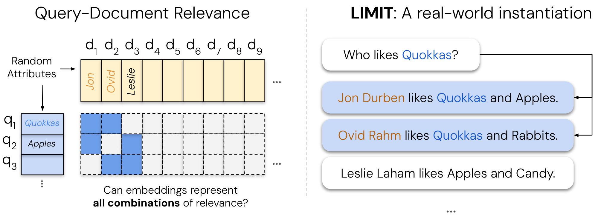
The authors combined mathematical proofs from linear algebra with empirical tests. They derived a lower bound on the dimension needed to separate all possible top-k document groups with a safety margin, using data from corpora up to billions of documents and typical k values like 10 or 100. To test this in the best-case scenario, they optimized embeddings directly on test data without language constraints, tracking when performance breaks as document count grows. They then built the LIMIT dataset: a realistic set of 50,000 short user profiles (documents) describing likes and dislikes for 1,850 items, paired with 1,000 simple queries like "who likes apples?" Each query targets exactly two relevant profiles from a dense 46-document subset, stressing all possible pairs without relying on complex logic. State-of-the-art models from Google, Meta, and others were evaluated, alongside alternatives like keyword-based BM25.

Key findings center on inescapable capacity limits. First, theory proves that for a million documents and top-10 retrieval, embeddings need at least 52 dimensions to cover all combinations with a 0.2 score margin; for billion-scale corpora and top-100, this jumps to over 700, exceeding typical sizes of 1,000–4,000 used in practice. Second, even ideal optimization on test data confirms this: performance holds for up to about 250 million documents at 4,096 dimensions but collapses beyond, following a polynomial growth pattern roughly 4–5 times stricter than theory due to optimization realities. Third, on LIMIT, top models like Gemini Embeddings and Qwen3 achieve under 20% recall at 100 results on the full set and fail to reach 90% even at 20 results on the small 46-document version—despite the task's simplicity. Fourth, instruction-tuned models fare slightly better than others, but all single-vector approaches lag far behind sparse keyword methods (BM25 hits 94% recall@100) and multi-vector models (around 55%). Finally, a powerful reranker like Gemini-2.5-Pro solves LIMIT perfectly in one pass, highlighting that the issue is specific to single-vector retrieval.

These results mean single-vector embeddings cannot represent the full range of relevance patterns needed for advanced tasks, especially as queries link unrelated documents via instructions or logic, leading to incomplete or wrong results. This raises risks in safety-critical applications like medical search, where missing key combinations could overlook vital information, and increases costs through reliance on larger models or post-retrieval fixes like reranking, which slow down systems. Unlike expectations from benchmark successes, where models overfit to limited queries, embeddings fail here on straightforward preferences—suggesting current training overlooks dense interconnection patterns common in real queries.

Leaders should shift away from single-vector embeddings for instruction-heavy retrieval, opting instead for hybrid systems: use them for initial broad filtering, then apply rerankers or multi-vector models for precision, trading some speed for accuracy. For web-scale needs, prioritize sparse or multi-vector architectures like ColBERT, which handle more combinations without exploding dimensions. To address gaps, pilot evaluations on LIMIT-like datasets during model development and explore dimension-efficient techniques like hypernetworks. If full reliability is required, invest in cross-encoder rerankers, though they limit scalability.

While the theory applies broadly to single-vector setups and empirical tests use diverse state-of-the-art models over 2024–2025 periods, limitations include a focus on text-only tasks and assumptions of perfect margins; multi-vector or sparse models face different constraints, and exact failure patterns remain unpredictable. Confidence is high in the core limits for current paradigms, but caution is advised for non-text domains or partial-coverage scenarios needing further bounds.

1. Introduction

Section Summary: Over the past two decades, information retrieval systems have evolved from simple keyword-matching methods like BM25 to advanced neural language models that represent entire texts as single vector embeddings, enabling them to handle increasingly complex searches, including those with custom definitions of relevance. This paper examines the fundamental mathematical limits of these embedding models, drawing on linear algebra to prove that no matter how they're trained, a fixed embedding dimension can't represent every possible combination of relevant documents for a given query, leading to inherent retrieval failures. To demonstrate this, the authors create an optimized test scenario and a simple real-world dataset called LIMIT, which even top-performing models struggle with, urging the field to recognize these boundaries and explore alternatives like multi-vector approaches for handling diverse, instruction-based queries.

Over the last two decades, information retrieval (IR) has moved from models dominated by sparse techniques (such as BM25 [1]) to those that use neural language models (LM) as their backbones ([2, 3, 4, 5]). These neural models are predominantly used in a single vector capacity, where they output a single embedding representing the entire input (also known as dense retrieval). These embedding models are capable of generalizing to new retrieval datasets and have been tasked with solving increasingly complicated retrieval problems ([6, 7, 8]).

In recent years this has been pushed even further with the rise of instruction-following retrieval benchmarks, where models are asked to represent any relevance definition for any query ([9, 10, 11, 12, 13]). For example, the QUEST dataset ([14]) uses logical operators to combine different concepts, studying the difficulty of retrieval for complex queries (e.g., "Moths or Insects or Arthropods of Guadeloupe"). On the other hand, datasets such as BRIGHT ([13]) explore the challenges arising from different definitions of relevance by defining relevance in ways that require reasoning. One subtask includes reasoning over a given Leetcode problem (the query) to find other Leetcode problems that share a subtask (e.g. others problems using dynamic programming). Although models cannot solve these benchmarks yet, the community has proposed these problems in order to push the boundaries of what dense retrievers are capable of—which is now implicitly every task that could be defined.

Rather than proposing empirical benchmarks to gauge what embedding models can achieve, we seek to understand at a more fundamental level what the limitations are. Since embedding models use vector representations in geometric space, there exist well-studied fields of mathematical research ([15]) that could be used to analyze these representations.

Our work aims to bridge this gap, connecting known theoretical results in linear algebra with modern advancements in neural information retrieval. We draw upon research in high-dimensional geometry to provide a lower bound on the embedding dimension needed to represent a given combination of relevant documents and queries. Specifically, we show that for a given embedding dimension $d$ there exist top- $k$ combinations of documents that cannot be returned—no matter the query—highlighting a theoretical and fundamental limit to embedding models.

To show that this theoretical limit is true for any retrieval model or training dataset, we test a setting where the vectors themselves are directly optimized with the test data. This allows us to empirically show how the embedding dimension enables the solving of retrieval tasks. We find that there exists a crucial point for each embedding dimension ($d$) where the number of documents is too large for the embedding dimension to encode all combinations. We then gather these crucial points for a variety of $d$ and show that this relationship can be modeled empirically with a polynomial function.

We also go one step further and construct a realistic but simple dataset based on these theoretical limitations (called LIMIT).[^2] Despite the simplicity of the task (e.g., who likes Apples? and Jon likes Apples, ...), we find it is very difficult for even state-of-the-art embedding models ([8, 16]) on MTEB ([7]), and practically impossible for models with small embedding dimensions using standard optimization techniques.

[^2]: Data and code are available at https://github.com/google-deepmind/limit

Overall, our work contributes: (1) a theoretical basis for the fundamental limitations of embedding models, (2) a best-case empirical analysis showing that this proof holds for any dataset instantiation (by free embedding optimization), and (3) a simple real-world natural language instantiation called LIMIT that even state-of-the-art embedding models cannot solve.

These results imply interesting findings for the community: on one hand we see neural embedding models becoming immensely successful. However, academic benchmarks test only a small amount of the queries that could be issued (and these queries are often overfitted to), hiding these limitations. Our work shows that as the tasks given to embedding models require returning ever-increasing combinations of top- $k$ relevant documents (e.g., through instructions connecting previously unrelated documents with logical operators), we will reach a limit of combinations they can represent.

Thus, the community should be aware of these limitations, both when creating evals and also by using alternate architectures—such as cross-encoders / multi-vector / more expressive similarity functions —when trying to handle the full range of instruction queries, i.e. any query and relevance definition.

2. Related Work

Section Summary: Recent years have seen rapid advancements in neural embedding models, evolving from basic text search to sophisticated systems that handle instructions and multiple data types like images and text, with examples including models like CoPali and Gemini Embeddings. These developments have pushed retrieval systems to manage diverse topics, complex instructions, and even logical reasoning, connecting previously unrelated information and highlighting the need to explore the fundamental limits of what these models can represent. Building on a long history of mathematical research into nearest neighbors and geometric spaces, the work draws theoretical insights from concepts like sphere-packing to determine the minimum embedding dimensions required for accurate retrieval across all possible scenarios, differing from prior studies that focused on sufficient dimensions or empirical constraints.

2.1 Neural Embedding Models

There has been immense progress on embedding models in recent years ([2, 3, 17]), moving from simple web search (text-only) to advanced instruction-following and multi-modal representations. These models generally followed advancements in language models, such as pre-trained LMs ([18]), multi-modal LMs ([19, 20]), and advancements in instruction-following ([21, 22]). Some of the prominent examples in retrieval include CoPali ([23]) and DSE ([24]) which focus on multimodal embeddings, Instructor ([25]) and FollowIR ([26]) for instruction following, and GritLM ([27]) and Gemini Embeddings ([8]) for pre-trained LMs turned embedders.

Our work, though focused solely on textual representations for simplicity, applies to all modalities of single vector embeddings for any domain of dataset. As the space of things to represent grows (through instructions or multi-modality) they will increasingly run into these theoretical limitations.

2.2 Empirical tasks pushing the limits of dense retrieval

Retrieval models have been pushed beyond their initial use cases to handle a broad variety of areas. Notable works include efforts to represent a wide group of domains ([6, 28]), a diverse set of instructions ([26, 29, 30, 31]), and to handle reasoning over the queries ([12, 13]). This has pushed the focus of embedding models from basic keyword matching to embeddings that can represent the full semantic meaning of language. As such, it is more common than ever to connect what were previously unrelated documents into the top- $k$ relevant set, [^3] increasing the number of combinations that models must be able to represent. This has motivated our interest in understanding the limits of what embeddings can represent, as current work expects it to handle every task.

[^3]: You can imagine an easy way to connect any two documents merely by using logical operators, i.e. X and Y.

Previous work has explored empirically the limits of models: [32] showed that smaller dimension embedding models have more false positives, especially with larger-scale corpora. [33] showed the empirical limitations of models in the cross-lingual setting and [34] showed how embedding dimensions relate to the bias-variance tradeoff. In contrast, our work provides a theoretical connection between the embedding dimension and the top-k sets it can retrieve, while also showing empirical limitations.

2.3 Theoretical Limits of Vectors in Geometric Space

Understanding and finding nearest neighbors in semantic space has a long history in mathematics research, with early work such as the Voronoi diagram being studied as far back as 1644 and formalized in 1908 ([35]). The order- $k$ version of the Voronoi diagram (i.e. the Voronoi diagram partitioning the space into regions based on their closest $k$ points) is obviously connected to information retrieval and has been studied for many years ([36]). The number of such regions is equal to the number of unique retrieval sets of size $k$, however this quantity is notoriously difficult to bound tightly ([37, 38, 39]).

We approach this problem from a different angle, asking not how many $k$-subsets a given configuration realizes, but rather what embedding dimension is necessary to realize all $k$-subsets with a guaranteed score margin. By applying a classical sphere-packing volume argument ([40, 41]), we obtain a lower bound on the embedding dimension in terms of $n$, $k$, and the margin $\gamma$. Our result is conceptually related to the Johnson–Lindenstrauss lemma ([42]), which gives a sufficient dimension to preserve pairwise distances among $n$ points; in contrast, our bound gives a necessary dimension to realize all retrieval sets with a margin. The role of the margin in controlling the complexity of realizable configurations also parallels classical results in statistical learning theory, including the fat-shattering dimension ([43]) and margin-based generalization bounds for linear classifiers ([44, 45]), where larger margins similarly constrain the capacity of the hypothesis class.

3. Representational Capacity of Vector Embeddings

Section Summary: This section explores the smallest dimension needed for vector embeddings to accurately retrieve specific sets of documents from large collections, using ideas from geometry to set a fundamental lower limit. It shows that to reliably separate relevant documents from irrelevant ones with a clear margin of separation, the embedding space must grow significantly with the size of the collection and the number of desired items, often requiring thousands of dimensions even for moderate margins. In practice, real-world search systems use far fewer dimensions to save space and speed, suggesting they fall short of this theoretical minimum and would need even more when accounting for learning challenges and data noise.

In this section we formally define the minimum embedding dimension required to satisfy a given retrieval objective, and draw on classical sphere-packing results from high-dimensional geometry to establish a lower bound. We note that this will be an extreme lower bound, as practical models have to deal with other constraints such as learning through gradient descent and using LM tokenization.

Setup.

Let $v_1, \dots, v_n\in\mathbb{R}^d$ be unit[^4] document vectors, and let queries be unit vectors $u\in\mathbb{R}^d$. Fix $\gamma>0$. A $k$-subset $S\subseteq[n]$ is realized with margin $\gamma$ if there exists a unit query $u_S$ such that

[^4]: For simplicity, as nearly all SoTA retrieval models use unit vectors.

$ \min_{i\in S}\langle u_S, v_i\rangle\ \ge\ \max_{j\notin S}\langle u_S, v_j\rangle\ +\ 2\gamma.\tag{1} $

Since $\langle u, v_i\rangle\in[-1, 1]$ for unit vectors, any score gap is at most $2$, hence equation 1 is feasible only for $0<\gamma\le 1$. Throughout, $\log$ denotes the natural logarithm.

Theorem 1: Dimension lower bound

Assume $1\le k<n$ and that every $k$-subset $S\subseteq[n]$ is realized with margin $\gamma$ as in equation 1. Then

$ \binom{n}{k}\ \le\ \Bigl(1+\frac{1}{\gamma}\Bigr)^{d}, \qquad\text{hence}\qquad d\ \ge\ \frac{\log\binom{n}{k}}{\log!\bigl(1+1/\gamma\bigr)}.\tag{2} $

Proof: Fix two distinct $k$-subsets $S\neq T$ and choose $i\in S\setminus T$ and $j\in T\setminus S$. Applying equation 1 to $S$ and to $T$ gives

$ \langle u_S, v_i-v_j\rangle\ge 2\gamma, \qquad \langle u_T, v_j-v_i\rangle\ge 2\gamma. $

Adding yields $\langle u_S-u_T, v_i-v_j\rangle\ge 4\gamma$. By Cauchy–Schwarz and (universally, for any unit vectors) $|v_i-v_j|\le |v_i|+|v_j|=2$, we obtain $|u_S-u_T|\ge 2\gamma$. Thus the $M=\binom{n}{k}$ unit queries ${u_S}$ are pairwise $2\gamma$-separated, so the open balls $B(u_S, \gamma)$ are disjoint. Moreover, since $|u_S|=1$, each $B(u_S, \gamma)\subseteq B(0, 1+\gamma)$, and therefore

$ M\cdot \mathrm{vol}!\bigl(B_d(\gamma)\bigr)\ \le\ \mathrm{vol}!\bigl(B_d(1+\gamma)\bigr). $

Using $\mathrm{vol}(B_d(r))=C_d, r^d$ for a constant $C_d$ depending only on $d$ (which cancels), we get $M\gamma^d\le (1+\gamma)^d$, i.e. $\binom{n}{k}\le \bigl((1+\gamma)/\gamma\bigr)^d=\bigl(1+1/\gamma\bigr)^d$. Rearranging yields equation 2.

:Table 1: Lower bounds for embedding dimension from Theorem 1 for $\gamma=0.1$. When n and k are both 1000, the result is trivial because $\binom{1000}{1000}=1 ($ there is only one k-subset, hence no "irrelevant" items to separate). We see for large k and n values these dimension requirements are already greater than those currently used for web-scale search. If these numbers are inflated by a small multiple due to constraints on gradient learning or other LM-based constraints (e.g. tokenization, generalization) these bounds are outside of any reasonable embedding dimension.

Corpus size $n$	$k=2$	$k=10$	$k=100$	$k=1000$
$10^2$	4	13	trivial	—
$10^3$	6	23	135	trivial
$10^4$	8	33	233	1354
$10^5$	10	42	329	2334
$10^6$	12	52	425	3296
$10^7$	14	61	521	4257
$10^8$	16	71	617	5217
$10^9$	17	81	713	6177
$10^{10}$	19	90	809	7137
$10^{11}$	21	100	905	8098

3.1.1 Implications

Numerical instantiation

We can illustrate the effects of this lower bound using $\gamma=0.1$ (score gap $2\gamma=0.2$), which is approximately standard for models based on empirical usage. Thus, equation 2 becomes $d\ge \left\lceil \log\binom{n}{k}/\log 11\right\rceil$, with a table for various $k$ and $n$ values in Table 1.

For $n\gg k$, $\log\binom{n}{k}\approx k\log(en/k)$, so equation 2 forces

$ d\ =\ \Omega!\left(\frac{k\log(en/k)}{\log(1+1/\gamma)}\right). $

A stricter margin requirement (larger $\gamma$) demands higher dimension, since $\log(1+1/\gamma)$ decreases with $\gamma$ (feasibility requires $\gamma\le 1$, so the denominator is at least $\log 2$).

Consequences

Due to space and speed requirements, most embeddings used for web-scale search are quantized or truncated (e.g. through Matryoshka embeddings ([46])) to less than 1k dimensions, while the largest embeddings used in research are around 4096 ([16]). We see that even with a moderate margin, which is needed to handle noise from messy data or quantization, the lower bounds in Table 1 can already be larger than what is used in practice.

Additional constraints on real-world models (such as needing to generalize, learn from gradient descent, and use natural language and tokenization) will make the dimension required in practice much higher. As Table 1 shows, even a small multiple of this lower bound would make the embedding dimension requirement infeasible. This multiple seems well-founded, as we will show in the next section from the best-case optimization setting (e.g. free embeddings).

4. Empirical Connection: Best Case Optimization

Section Summary: To test the theoretical limits of embedding models empirically, researchers created an ideal "free embedding" setup where document and query vectors could be directly optimized using gradient descent, without any real-world language constraints, to represent the absolute best-case performance. They generated random sets of documents and queries focused on top-2 relevance pairs, then used optimization techniques to push until the model failed to perfectly distinguish all combinations, identifying a breaking point called the "critical-n" based on embedding dimension. The results, extrapolated via a polynomial curve, reveal that even this optimized scenario requires much larger dimensions than current models provide—such as over 4 million for embedding sizes around 1,000—to handle web-scale search with millions of documents, confirming that real embedding systems fall short.

Having established a theoretical limitation of embedding models based on their embedding dimension $d$, we seek to show that this holds empirically also.

To show the strongest optimization case possible, we design experiments where the vectors themselves are directly optimizable with gradient descent.[^5] We call this "free embedding" optimization, as the embeddings are free to be optimized and not constrained by natural language, which imposes constraints on any realistic embedding model. Thus, this shows whether it is feasible for any embedding model to solve this problem: if the free embedding optimization cannot solve the problem, real retrieval models will not be able to either. It is also worth noting that we do this by directly optimizing the embeddings over the target qrel matrix (test set). This will not generalize to a new dataset, but is done to show the highest performance that could possibly occur.

[^5]: This could also be viewed as an embedding model where each query/doc are a separate vector via lookup.

Experimental Settings

We create a random document matrix (size $n$) and a random query matrix with top- $k$ sets (of all combinations, i.e. size $m=\binom{n}{k}$), both with unit vectors. We then directly optimize for solving the constraints with the Adam optimizer ([47]).[^6] Each gradient update is a full pass through all correct triples (i.e. full dataset batch-size) with the InfoNCE loss function ([48]), [^7] with all other documents as in-batch negatives (i.e. full dataset in batch). As nearly all embedding models use normalized vectors, we do also (via projected gradient descent). We perform early stopping when there is no improvement in the loss for 1000 iterations. We gradually increase the number of documents (and thus the binomial amount of queries) until the optimization is no longer able to solve the problem (i.e. achieve 100% accuracy). We call this the critical-n point.

[^6]: We found similar results with SGD, but we use Adam for speed and similarity with existing training methods.

[^7]: In preliminary experiments, we found that InfoNCE performed best, beating MSE and Margin. As we are directly optimizing the vectors with full-dataset batches, this is $\mathcal{L}{\text{total}} = -\frac{1}{M} \sum{i=1}^{M} \log \frac{\sum_{d_r \in R_i} \exp(\text{sim}(q_i, d_r) / \tau)}{\sum_{d_k \in D} \exp(\text{sim}(q_i, d_k) / \tau)}$ where $D$ is all docs, $d_r$ is the relevant documents for query $q_i$ and $d_k$ are the non-relevant documents. For experiments with sigmoid learning functions (e.g. [49], see Appendix C)

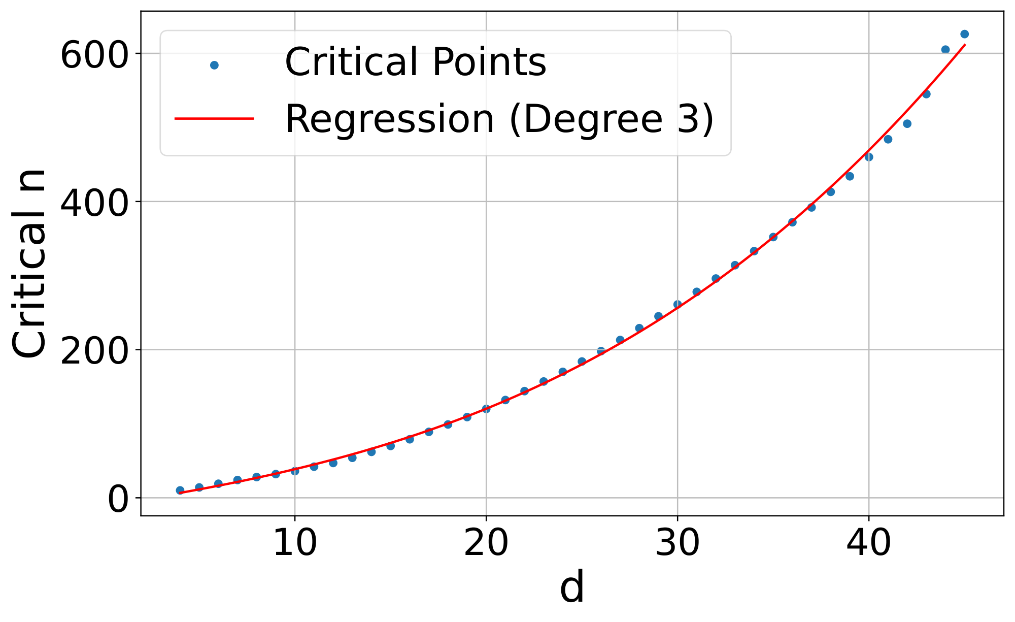
We focus on relatively small sizes for $n$, $k$, and $d$ due to the combinatorial explosion of combinations with larger document values (i.e. 50k docs with top- $k$ of 100 gives 7.7e+311 combinations, which would be equivalent to the number of query vectors of dimension $d$ in that free embedding experiment). We use $k=2$ and increase $n$ by one for each $d$ value until it breaks. We fit a polynomial regression line to the data so we can model and extrapolate results outwards.

Results

Figure 2 shows that the curve fits a 3rd degree polynomial curve, with formula $y=-10.5322 + 4.0309d + 0.0520d^2 + 0.0037d^3$ ($r^2$ =0.999). Extrapolating this curve outward gives the critical-n values (for embedding size): 500k (512), 1.7m (768), 4m (1024), 107m (3072), 250m (4096). We note that this is the best case: a real embedding model cannot directly optimize the query and document vectors to match the test qrel matrix (and is constrained by factors such as "modeling natural language"). The results also show that the lower bounds in the previous section are a gross underestimate of real-world performance, as Table 1 shows a lower bound of 4 for $n=100$ whereas we see the free embeddings needing $d>18$ (e.g. a 4.5 multiplier even in the no-generalization or natural language case). Overall, these numbers already show that for web-scale search, even the largest embedding dimensions with ideal test-set optimization are not enough to model all combinations.

5. Empirical Connection: Real-World Datasets

Section Summary: This section explains how the study's theoretical findings about embedding models apply to real-world data, noting that existing retrieval datasets like QUEST use only a tiny fraction of possible queries due to the high cost of creating and annotating them, even though the potential combinations of relevant documents are astronomically vast. To address this, the authors introduce the LIMIT dataset, a simple synthetic collection of 50,000 short documents about people's preferences for everyday items, paired with 1,000 straightforward queries asking who likes a specific thing, designed to test all possible pairs of relevant documents from a core set of 46 items. When evaluating top state-of-the-art embedding models on LIMIT, the results show these models struggle significantly despite the task's simplicity, with performance improving only somewhat as model complexity or dimensionality increases, while simpler lexical methods like BM25 perform surprisingly well.

The free embedding experiments provide empirical evidence that our theoretical results hold true. However, they still are abstract - what does this mean for real embedding models? In this section we (1) draw connections from this theory to existing datasets and (2) create a trivially simple yet extremely difficult retrieval task for existing SOTA models.

5.1 Connection to Existing Datasets

Existing retrieval datasets typically use a static evaluation set with limited numbers of queries, as relevance annotation is expensive to do for each query. This means practically that the space of queries used for evaluation is a very small sample of the number of potential queries. For example, the QUEST dataset ([14]) has 325k documents and queries with 20 relevant documents per query, with a total of 3357 queries. The number of unique top-20 document sets that could be returned with the QUEST corpus would be $\binom{325k}{20}$ which is equal to 7.1e+91 (larger than the estimate of atoms in the observable universe, $10^{82}$). Thus, the 3k queries in QUEST can only cover an infinitesimally small part of the qrel combination space.

Although it is not possible to instantiate all combinations when using large-scale corpora, search evaluation datasets are a proxy for what any user would ask for and ideally would be designed to test many combinations, as users will do. In many cases, developers of new evaluations simply choose to use fewer queries due to cost or computational expense of evaluation. For example, QUEST's query "Novels from 1849 or George Sand novels" combines two categories of novels with the "OR" operator – one could instantiate new queries to relate concepts through OR'ing other categories together. Similarly, with the rise of search agents, we see greater usage of hyper-specific queries: BrowseComp ([50]) has 5+ conditions per query, including range operators. With these tools, it is possible to sub-select any top- $k$ relevant set with the right operators if the documents are sufficiently expressive (i.e. non-trivial). Thus, that existing datasets choose to only instantiate some of these combinations is mainly for practical reasons and not because of a lack of existence.

In contrast to these previous works, we seek to build a dataset that evaluates all combinations of top- $k$ sets for a small number of documents. Rather than using difficult query operators like QUEST, BrowseComp, etc. (which are already difficult for reasons outside of the qrel matrix) we choose very simple queries and documents to highlight the difficulty of representing all top- $k$ sets themselves.

5.2 The LIMIT Dataset

Dataset Construction

In order to have a natural language version of this dataset, we need some way to map combinations of documents into something that could be retrieved with a query. One simple[^8] way to do this is to create a synthetic version with latent variables for queries and documents and then instantiate it with natural language. For this mapping, we choose to use attributes that someone could like (i.e. Jon likes Hawaiian pizza, sports cars, etc.) as they are plentiful and don't present issues w.r.t. other items: one can like Hawaiian pizza but dislike pepperoni, all preferences are valid. We then enforce two constraints for realism: (1) users shouldn't have too many attributes, thus keeping the documents short (less than 50 per user) and (2) each query should only ask for one item to keep the task simple (i.e. "who likes X"). We gather a list of attributes a person could like through prompting Gemini 2.5 Pro. We then clean it to a final 1850 items by iteratively asking it to remove duplicates/hypernyms, while also checking the top failures with BM25 to ensure no overlap.

[^8]: This is just one way, designed to be realistic and simple. However, our framework allows for any way of instantiation – not stuck to this arbitrary natural language design.

We choose to use 50k documents in order to have a hard but relatively small corpus and 1000 queries to maintain statistical significance while still being fast to evaluate. For each query, we choose to use two relevant documents (i.e. $k$ =2), both for simplicity in instantiating and to mirror previous work (i.e. NQ, HotpotQA, etc. ([51, 52])).

Our last step is to choose a qrel matrix to instantiate these attributes. Although we could not prove the hardest qrel matrix definitively with theory, we intuit that our theoretical results imply that the more interconnected the qrel matrix is (e.g. dense with all combinations) the harder it would be for models to represent. Following this, we use the qrel matrix with the highest number of documents for which all combinations would be just above 1000 queries for a top- $k$ of 2 (46 docs, since $\binom{46}{2}$ is 1035, the smallest above 1k).

We then assign random natural language attributes to the queries, adding these attributes to their respective relevant documents (c.f. Figure 1). We give each document a random first and last name from open-source lists of names. Finally, we randomly sample new attributes for each document until all documents have the same number of attributes. As this setup has many more documents than those that are relevant to any query (46 relevant documents, 49.95k non-relevant to any query) we also create a "small" version with only the 46 documents that are relevant to one of the 1000 queries.

Models We evaluate the state-of-the-art embedding models including GritLM ([27]), Qwen 3 Embeddings ([16]), Promptriever ([53]), Gemini Embeddings ([8]), Snowflake's Arctic Embed Large v2.0 ([54]), and E5-Mistral Instruct ([5, 55]). These models range in embedding dimension (1024 to 4096) as well as in training style (instruction-based, hard negative optimized, etc.). We also evaluate three non-single vector models to show the distinction: BM25 ([1, 56]), gte-ModernColBERT ([57, 58]), and a token-wise TF-IDF.[^9]

[^9]: This model turns each unique item into a token and then does TF-IDF. We build it to show that it gets 100% on all tasks (as it reverse engineers our dataset construction) and thus we do not include it in future charts.

We show results at the full embedding dimension and also with truncated embedding dimension (typically used with matryoshka learning, aka MRL ([46])). For models not trained with MRL this will result in sub-par scores, thus, models trained with MRL are indicated with stars in the plots. However, as there are no LLMs with an embedding dimension smaller than 384, we include MRL for all models to small dimensions (32) to show the impact of embedding dimensionality.

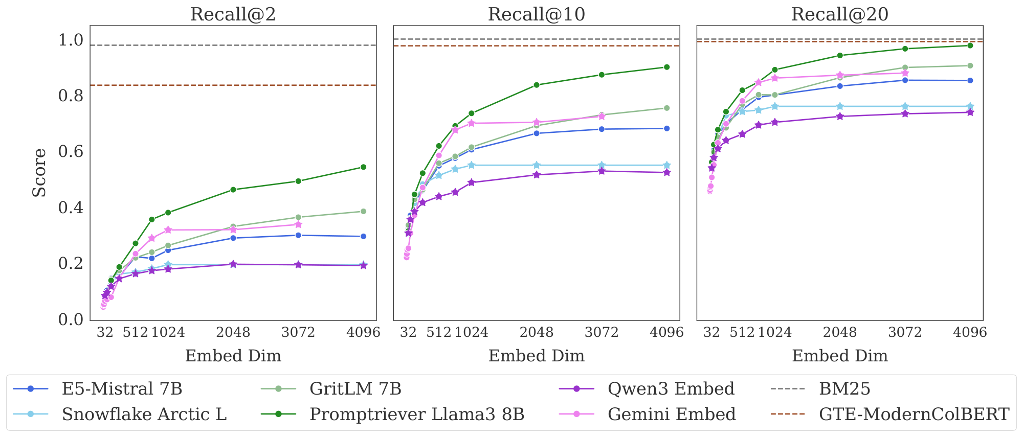
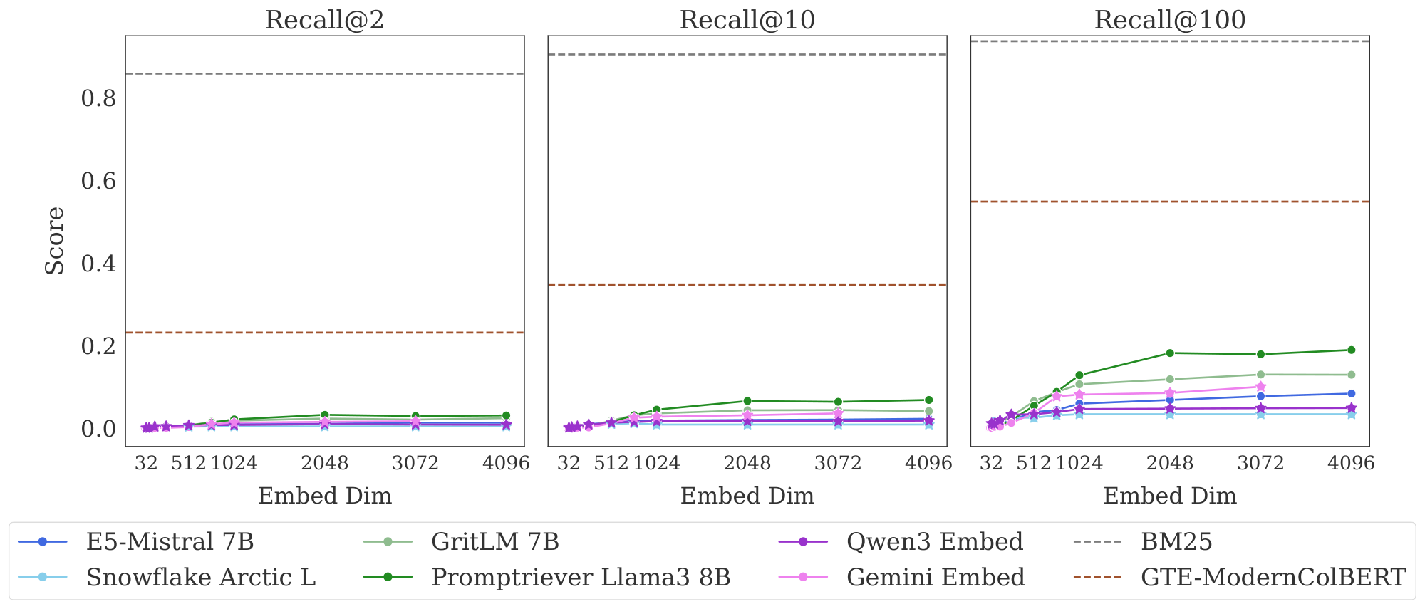
Results Figure 3 shows the results on the full LIMIT while Figure 4 shows the results on the small (46 document) version.

The results are surprising - models severely struggle even though the task is trivially simple. For example, in the full setting models struggle to reach even 20% recall@100 and in the 46 document version models cannot solve the task even with recall@20.

We see that model performance depends crucially on the embedding dimensionality (better performance with bigger dimensions). Interestingly, models trained with more diverse instruction, such as Promptriever, perform better, perhaps because their training allows them to use more of their embedding space (compared to models which are trained with MRL and on a smaller range of tasks that can perhaps be consolidated into a smaller embedding manifold).

For alternative architectures, GTE-ModernColBERT does significantly better than single-vector models (although far from solving the task) while BM25 comes close to perfect scores. Both of these alterative architectures (sparse and multi-vector) offer various trade-offs, see Section 5.3 for analysis.

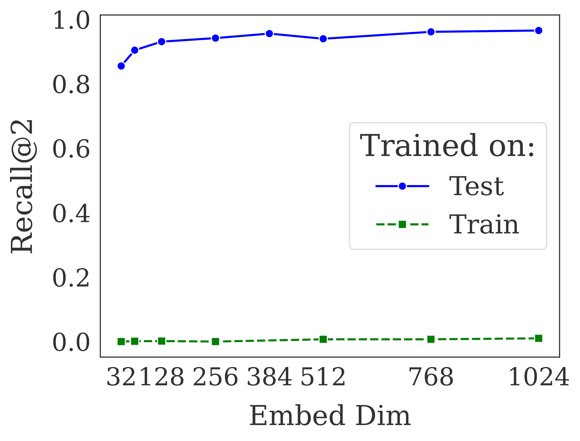
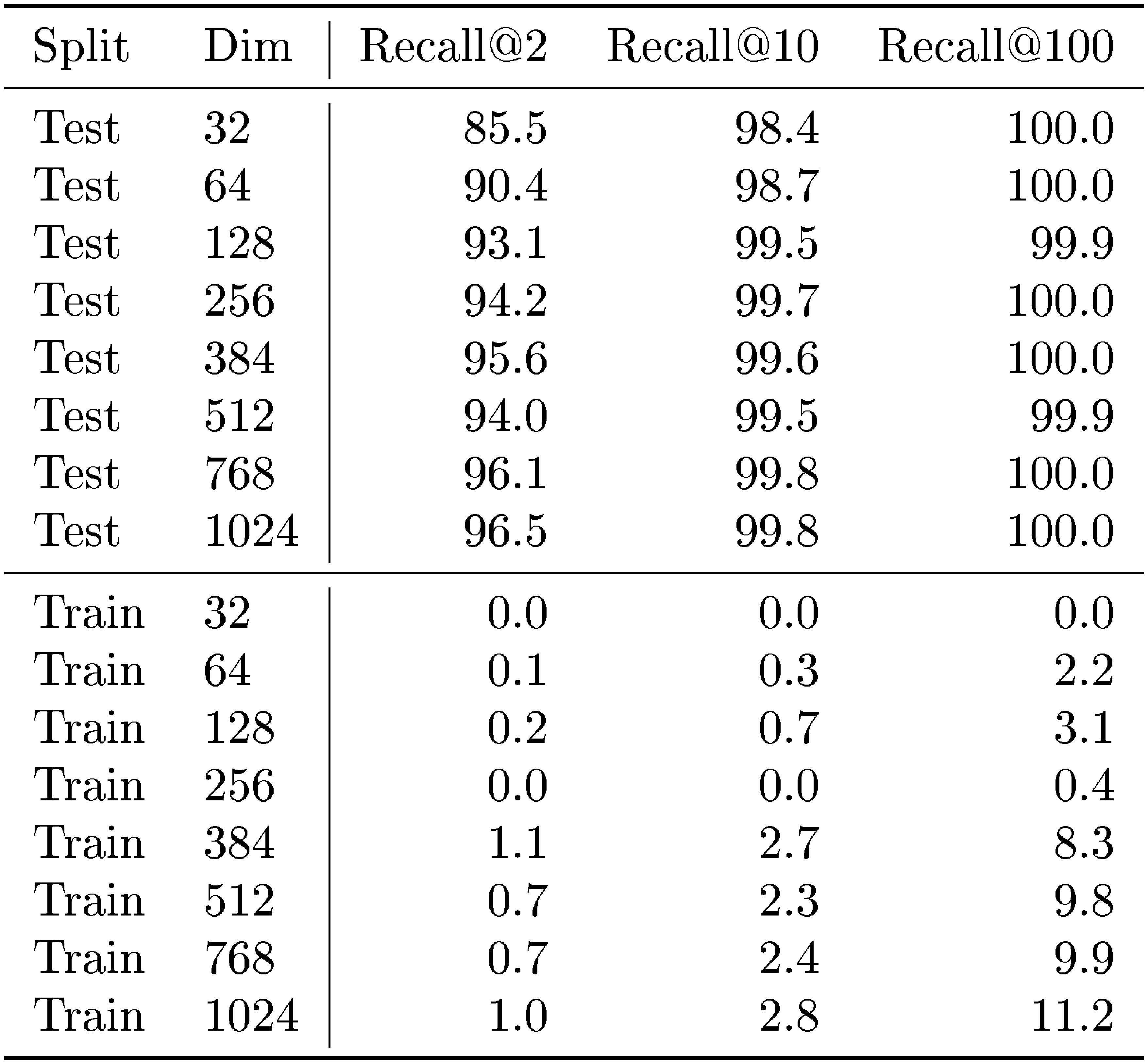
Is this Domain Shift? Although our queries look similar to standard web search queries, we wondered whether there could be some domain shift causing the low performance. If so, we would expect that training on a training set of similar examples would significantly improve performance. On the other hand, if the task was intrinsically hard, training on the training set would provide little help whereas training on the test set would allow the model to overfit to those tokens (similar to the free embeddings).

To test this we take an off-the-shelf embedding model and train it on either the training set (created synthetically using non-test set attributes) or the official test set of LIMIT. We use lightonai/modernbert-embed-large ([59]) and fine-tune it on these splits, using the full dataset for in batch negatives (excluding positives) using SentenceTransformers ([60]). We show a range of dimensions by projecting the hidden layer down to the specified size during training (rather than using MRL).

Figure 5 shows the model trained on the training set cannot solve the problem, although it does see very minor improvement from near zero recall@10 to up to 2.8 recall@10. The lack of performance gains when training in-domain indicate that poor performance is not due to domain shift. By training the model on the test set we see it can learn the task, overfitting on the tokens in the test queries. This aligns with our free embedding results, that it is possible to overfit to the $N=46$ version with only 12 dimensions. However, it is notable that the real models with 64 dimensions still cannot completely solve the task, implying real models perform significantly worse than the bounds shown in § 4.

What about Non-Lexical Matches? Our previous results show that lexical models greatly outperform their neural counterparts. However, this is not to imply that lexical models are a panacea - although they have higher dimensionality than single-vector models, they have other shortcomings.

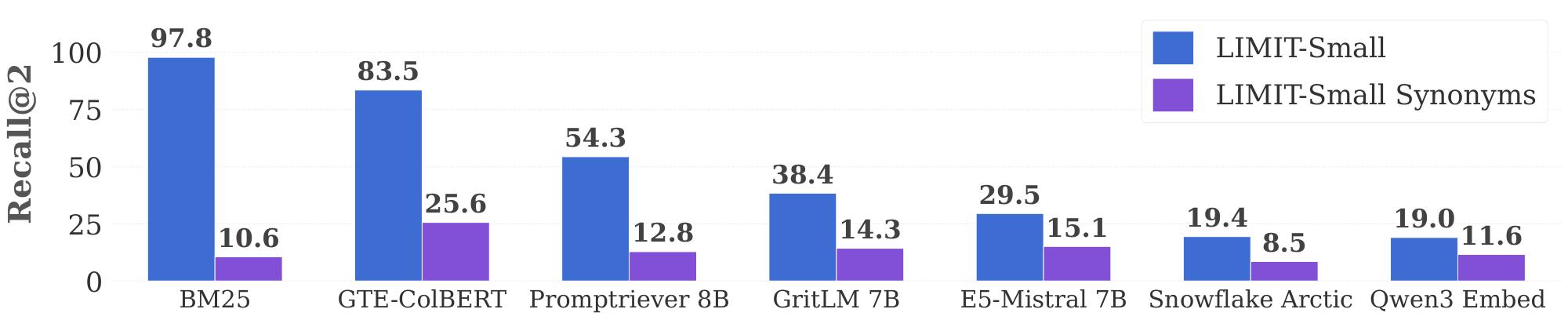
We illustrate this by creating a version of LIMIT-small that replaces all items in the corpus with their synonyms, reducing the amount of lexical overlap. We ask Gemini 2.5 Pro to come up with synonyms that don’t match any other existing synonyms or original items, by using either scientific names, similar meanings, or if necessary hypernyms. This creates a mapping like "glasses" to "spectacles", etc.[^10] We repeat the previous experiment on LIMIT-small (synonyms) and compare to LIMIT-small in Figure 6. We find that all models drop in performance as the task is now more difficult, but BM25 drops the most and now underperforms the neural models (e.g. BM25 drops more than 89% whereas Qwen3 embedding drops 38.9%). Thus, we can see that although lexical models have strengths like higher dimensionality, they are limited by their keyword-only matching ability. We expand more upon their strengths and weaknesses for instruction-following in Section 5.3.

[^10]: We note that it doesn't remove all lexical overlap due to items like “Scuba Diving” -> “Underwater Diving”

Implications Single-vector models are fundamentally limited by their embedding dimension. The LIMIT dataset is a particular instantiation, with very simple queries and documents, designed to highlight this property. This small version of LIMIT can be embedded in just 12 dimensions (as seen in the free embeddings experiments), yet all models fail to perform well, suggesting other architectural weaknesses. Irrespective of the architecture involved, however, our framework can scale the dataset's difficulty to consistently demonstrate this fundamental limitation.

5.3 Alternatives to Embedding Models

Our previous results show both theoretically and empirically that embedding models cannot represent all combinations of documents in their top- $k$ sets, making them unable to represent and solve some retrieval tasks. As current embedding models have grown larger (e.g. up to 4096), this has helped reduce negative effects for smaller dataset sizes. However, with enough combinations of top- $k$ sets the dimensionality would have to increase to an infeasible size for non-toy datasets. Thus, although they are useful for first stage results, more expressive retriever architectures will be needed.

Cross-Encoders Although not suitable for first stage retrieval at scale, they are already typically used to improve first stage results. Is LIMIT challenging for rerankers also? We evaluate a long context reranker, Gemini-2.5-Pro ([61]) on the small setting as a comparison. We give Gemini all 46 documents and all 1000 queries at once, asking it to output the relevant documents for each query with one generation. We find that it can successfully solve (100%) all 1000 queries in one forward pass. This is in contrast to even the best embedding models with a recall@2 of less than 60% (Figure 4). Thus we can see that LIMIT is easy for state-of-the-art reranker models, which do not have the same limitations based on embedding dimension.

Multi-vector models Multi-vector models are more expressive through the use of multiple vectors per sequence combined with the MaxSim operator ([62]). These models show promise on the LIMIT dataset, with scores greatly above the single-vector models despite using a smaller backbone (ModernBERT, [63]). However, these models are not generally used for instruction-following or reasoning-based tasks (see [64] as one of the few that exist), leaving it an open question to how well multi-vector techniques will transfer to these tasks.

Sparse models Sparse models (both lexical and neural) can be thought of as single vectors but with very high dimensionality. This dimensionality helps BM25 avoid the problems of the neural embedding models as seen in Figure 3. Since the $d$ of their vectors is high, they can scale to many more combinations than their dense vector counterparts. However, it is less clear how to apply sparse models to instruction-following and reasoning-based tasks where there is no lexical or even paraphrase-like overlap. We leave this direction (and hybrid sparse/dense solutions) to future work.

We note that all of these options have various trade-offs and none provide a clear path to solving this problem as-is. We leave it to future work to develop new techniques to mitigate these issues: perhaps through one of these alterative categories or through new ideas around single-vector models that can resolve the underlying issue (potentially through techniques such as hyperencoders ([65]) or other future work on single vector architectures yet to be developed).

6. Conclusion

Section Summary: The LIMIT dataset reveals a key weakness in embedding models used for search and retrieval, showing that these models can't always rank the most relevant documents at the top due to limits in their fixed dimensional setup. Through theory and real-world tests, including tweaks to model vectors, the researchers prove this issue persists even in top-performing systems, using LIMIT as a simple example they fail to handle correctly. This suggests experts need to rethink how instruction-guided searches will shape next-generation retrieval tools.

We introduce the LIMIT dataset, which highlights a fundamental limitation of embedding models. We provide a theoretical connection which shows that, for a fixed embedding dimension there will be some set of documents such that certain sets are unattainable as top- $k$ sets. We show these theoretical results hold empirically, through best case optimization of the vectors themselves, and make a practical connection to existing state-of-the-art models by creating a realistic and simple instantiation of the theory, called LIMIT, that these models cannot solve. Our results imply that the community should reconsider how instruction-based retrieval will impact future retrievers.

Limitations

Section Summary: The study focuses on single-vector embedding models and may not apply to other types, like multi-vector ones, though some initial tests were done; deeper theoretical links for those are left for future research. It also lacks proofs for scenarios where models can make minor errors, such as missing just a few combinations, and points to other studies for that. While it proves certain data patterns can't be handled by these models, it can't specify which kinds will fail, meaning some tasks might work perfectly, but others are guaranteed to be impossible.

Although our experiments provide theoretical insight for the most common type of embedding model (single vector) they do not hold necessarily for other architectures, such as multi-vector models. Although we showed initial empirical results with non-single vector models, we leave it to future work to extend our theoretical connections to these settings. We also did not show theoretical results for the setting where the user allows some mistakes, e.g. capturing only the majority of the combinations. We leave putting a bound on this scenario to future work and would invite the reader to examine works like [66].

We have shown the theoretical connection that proves that some combinations cannot be represented by embedding models, however, we cannot prove apriori which types of combinations they will fail on. Thus, it is possible that there are some instruction-following or reasoning tasks they can solve perfectly, however, we do know that there exists some tasks that they will never be able to solve.

Acknowledgments

Section Summary: The authors express gratitude to Tanmaya Dabral, Zhongli Ding, Anthony Chen, Ming-Wei Chang, Kenton Lee, and Kristina Toutanova for their valuable feedback on the work. They also thank Kiril Bangachev, Guy Bresler, Iliyas Noman, Yury Polyanskiy, Antonio Vergari, Adam Lopez, and Andreas Grivas for providing useful guidance and references related to research on sign-rank.

We thank Tanmaya Dabral, Zhongli Ding, Anthony Chen, Ming-Wei Chang, Kenton Lee, and Kristina Toutanova for their helpful feedback. We thank Kiril Bangachev, Guy Bresler, Iliyas Noman, Yury Polyanskiy, Antonio Vergari, Adam Lopez, and Andreas Grivas for pointers to work on sign-rank.

Appendix

Section Summary: The appendix explores connections between the paper's findings on embedding models and prior work on order-k Voronoi regions, which count possible top-k retrieval results but are hard to compute in higher dimensions, leading the authors to adopt an alternative method. It details practical aspects like using standard evaluation settings for short documents, training with specific loss functions and batch sizes on powerful GPUs, and running experiments on various hardware for efficiency. Additionally, it discusses differences in loss functions between vision-language and text-only models, and provides theoretical proofs on embedding dimensions using concepts like sign-rank and order-preserving ranks to ensure relevant documents score higher than irrelevant ones.

A. Relationship to Order-K Voronoi Regions

We also provide an explanation for how our results compare to [36] which put bounds on the number of regions in the order- $k$ Voronoi graph. The order- $k$ Voronoi graph is defined as the set of points having a particular set of $n$ points in $S$ as its $n$ nearest neighbors. This maps nicely to retrieval, as each order- $k$ region is equivalent to one retrieved set of top- $k$ results. Then the count of unique regions in the Voronoi graph is the total number of combinations that could be returned for those points. However, creating an empirical order-k Voronoi graph is computationally infeasible for $d$ > 3, and theoretically it is hard to bound tightly. Thus we use a different approach for showing the limitations of embedding models.

B. Hyperparameter and Compute Details

Inference

We use the default length settings for evaluating models using the MTEB framework ([7]). As our dataset has relatively short documents (around 100 tokens), this does not cause an issue.

Training

For training on the LIMIT training and test set we use the SentenceTransformers library ([60]) using the MultipleNegativesRankingLoss. We use a full dataset batch size and employ the no duplicates sampler to ensure that no in-batch negatives are duplicates of the positive docs. We use a learning rate of 5e-5. We train for 5 epochs and limit the training set slightly to the size of the test set (from 2.5k to 2k examples, matching test).

Compute

Inference and training for LIMIT is done with A100 GPUs on Google Colab Pro. The free embedding experiments are done mainly on H100 GPUs and TPU v5's for larger size $N$ to accommodate higher VRAM for full-dataset batch vector optimization.

C. Sigmoid Loss Function for Free Embeddings

In concurrent work by [49], they show that for vision-language embedding models like CLIP (that more commonly use sigmoid loss functions) that the free-embedding experiments can be solved in fewer dimensions than in our setting (assuming no margin). As our results found the best performance with InfoNCE, which attempts to create the widest possible margin, this indicates that there are additional questions to resolve around learnability. We welcome further insight into this question both theoretically and empirically, as there exists widely disparate practices between the vision-language community (where sigmoid loss functions are often SOTA) and the text-only community (where sigmoid loss functions are almost never used due to worse performance).

This sigmoid learning is also closely related to other work, such as [67] and generally on the topic of work such as ([68, 69])

D. Proof using Sign-Rank

In the initial version of this paper, we provided a theoretical bound without any margin requirement based on the qrel matrices sign rank. Although the proof is correct, the sign rank of the $\binom{n}{k}$ matrix has been established in previous work ([70]) and only depends on k. We include the proof connecting notions relevant for retrieval with the classic notion of sign-rank, however we emphasize that this will provide a weaker requirement on dimension as it assumes no margin.

D.1 Formalization

We consider a set of $m$ queries and $n$ documents with a ground-truth relevance matrix $A \in {0, 1}^{m \times n}$, where $A_{ij} = 1$ if and only if document $j$ is relevant to query $i$.[^11] Vector embedding models map each query to a vector $u_i \in \mathbb{R}^d$ and each document to a vector $v_j \in \mathbb{R}^d$. Relevance is modeled by the dot product $u_i^T v_j$, with the goal that relevant documents should score higher than irrelevant ones.

[^11]: The matrix $A$ is often called the "qrels" (query relevance judgments) matrix in information retrieval.

Concatenating the vectors for queries in a matrix $U \in \mathbb R^{d \times m}$ and those for documents in a matrix $V \in \mathbb R^{d \times n}$, these dot products are the entries of the score matrix $B = U^TV$. The smallest embedding dimension $d$ that can realize a given score matrix is, by definition, the rank of $B$. Therefore, our goal is equivalent to finding the minimum rank of a score matrix $B$ that correctly orders documents according to the relevance specified in $A$, which we formalize in the following definition.

Definition

Given a matrix $A \in \mathbb R^{m \times n}$, the row-wise order-preserving rank of $A$ is the smallest integer $d$ such that there exists a rank- $d$ matrix $B$ that preserves the relative order of entries in each row of $A$. We denote this as

$ \operatorname{rank}\text{rop}A = \min {\operatorname{rank} B \mid B \in \mathbb R^{m \times n}, \text{ such that for all } i, j, k, \text{ if } A{ij} > A_{ik} \text{ then } B_{ij} > B_{ik}}. $

In other words, if $A$ is a binary ground-truth relevance matrix, $\operatorname{rank}_\text{rop} A$ is the minimum dimension necessary for any vector embedding model to return relevant documents before irrelevant ones for all queries. Alternatively, we might require that the scores of relevant documents can be cleanly separated from those of irrelevant ones by a threshold.

Definition

Given a binary matrix $A\in {0, 1}^{m \times n}$:

• The row-wise thresholdable rank of $A$ ($\operatorname{rank}\text{rt} A$) is the minimum rank of a matrix $B$ for which there exist row-specific thresholds ${\tau_i}{i=1}^m$ such that for all $i, j$, $B_{ij} > \tau_i$ if $A_{ij} = 1$ and $B_{ij} < \tau_i$ if $A_{ij} = 0$.
• The globally thresholdable rank of $A$ ($\operatorname{rank}\text{gt} A$) is the minimum rank of a matrix $B$ for which there exists a single threshold $\tau$ such that for all $i, j$, $B{ij} > \tau$ if $A_{ij} = 1$ and $B_{ij} < \tau$ if $A_{ij} = 0$.

Remark 2

This two-sided separation condition may be seen as slightly stronger than requiring $B_{ij} > \tau_i$ if and only if $A_{ij} = 1$, however since there are only finitely many elements of $B_{ij}$ we could always perturb the latter threshold by a sufficient number such that the two-sided condition holds.[^1]

[^1]: Without loss of generality, we may assume the thresholds in the above definitions are not equal to any elements of $B$ since we could increase the threshold of $\tau$ by a sufficiently small $\epsilon$ to preserve the inequality.

D.2 Theoretical Bounds

For binary matrices, row-wise ordering/thresholding are equivalent notions of representation capacity.

Proposition 3

For a binary matrix $A\in{0, 1}^{m \times n}$, we have that $\operatorname{rank}\text{rop} A = \operatorname{rank}\text{rt} A$.

Proof: ($\le$) Suppose $B$ and $\tau$ satisfy the row-wise thresholdable rank condition. Since $A$ is a binary matrix $A_{ij} > A_{ik}$ implies $A_{ij} = 1$ and $A_{ik} = 0$, thus $B_{ij} > \tau_i > B_{ik}$, and hence $B$ also satisfies the row-wise order-preserving condition.

($\ge$) Let $B$ satisfy the row-wise order-preserving condition, so $A_{ij} > A_{ik}$ implies $B_{ij} > B_{ik}$. For each row $i$, let $U_i = {B_{ij} \mid A_{ij}=1}$ and $L_i = {B_{ij} \mid A_{ij} = 0}$. The row-wise order-preserving condition implies that every element of $U_i$ is greater than every element of $L_i$. We can therefore always find a threshold $\tau_i$ separating them (e.g $\tau_i = (\max L_i + \min U_i) / 2$ if both are non-empty, trivial otherwise). Thus $B$ is also row-wise thresholdable to $A$.

The notions we have described so far are closely related to the sign rank of a matrix, which we use in the rest of the paper to establish our main bounds.

Definition: Sign Rank

The sign rank of a matrix $M \in {-1, 1}^{m\times n}$ is the smallest integer $d$ such that there exists a rank $d$ matrix $B \in \mathbb R^{m \times n}$ whose entries have the same sign as those of $M$, i.e.

$ \operatorname{rank}\pm{M} = \min {\operatorname{rank} B \mid B \in \mathbb R^{m \times n} \text{ such that for all } i, j \text{ we have } \operatorname{sign} B{ij} = M_{ij}}. $

In what follows, we use $\mathbf 1_n$ to denote the $n$-dimensional vector of ones, and $\mathbf 1_{m \times n}$ to denote an $m \times n$ matrix of ones.

Proposition 4

Let $A\in {0, 1}^{m \times n}$ be a binary matrix. Then $2A - \mathbf 1_{m \times n} \in {-1, 1}^{m \times n}$ and

$ \operatorname{rank}\pm (2A - \mathbf 1{m \times n}) - 1\le \operatorname{rank}\text{rop} A = \operatorname{rank}\text{rt} A \le \operatorname{rank}\text{gt} A \le \operatorname{rank}\pm (2A - \mathbf 1_{m \times n}) $

Proof: N.b. the equality was already shown in Proposition 3. We prove each inequality separately.

1. $\operatorname{rank}\text{rt} A \le \operatorname{rank}\text{gt} A$: True by definition, since any matrix satisfying the globally thresholdable condition trivially satisfies a row-wise thresholdable condition with the same threshold for each row.

2. $\operatorname{rank}\text{gt} A \le \operatorname{rank}\pm(2A-\mathbf 1_{m \times n})$: Let $B$ be any matrix whose entries have the same sign as $2A-\mathbf 1_{m \times n}$, then

$ B_{ij} > 0 \iff 2A_{ij}-1> 0 \iff A_{ij} = 1. $

Thus $B$ satisfies the globally thresholdable condition with a threshold of $0$.

3. $\operatorname{rank}_\pm(2A-\mathbf 1 {m \times n}) - 1 \le \operatorname{rank}\text{rt}A$: Suppose $B$ satisfies the row-wise thresholdable condition with minimal rank, so $\operatorname{rank}\text{rt} A = \operatorname{rank} B$ and there exists $\tau \in \mathbb R^m$ such that $B{ij} > \tau_i$ if $A_{ij} = 1$ and $B_{ij} < \tau_i$ if $A_{ij} = 0$. Then the entries of $B - \tau \mathbf 1_n^T$ have the same sign as $2A-\mathbf 1_{m \times n}$, since $(B - \tau \mathbf 1_n^T){ij} = B{ij} - \tau _i$ and

$ \begin{align} B_{ij} - \tau_i > 0 &\iff A_{ij} = 1 \iff 2A_{ij} - 1 > 0, \text{ and}\ B_{ij} - \tau_i < 0 &\iff A_{ij} = 0 \iff 2A_{ij} - 1 < 0. \end{align} $

Thus $\operatorname{rank}\pm(2A - \mathbf 1{m \times n}) \le \operatorname{rank}(B - \tau \mathbf 1_n^T) \le \operatorname{rank}(B) + \operatorname{rank}(\tau \mathbf 1_n^T) = \operatorname{rank}_\text{rt} A + 1$.

Combining these gives the desired chain of inequalities.

D.3 Consequences

In the context of a vector embedding model, this provides a lower and upper bound on the dimension of vectors required to exactly capture a given set of retrieval objectives, in the sense of row-wise ordering, row-wise thresholding, or global thresholding. In particular, given some binary relevance matrix $A\in {0, 1}^{m \times n}$, we need at least $\operatorname{rank}\pm (2A - \mathbf 1{m \times n}) - 1$ dimensions to capture the relationships in $A$ exactly, and can always accomplish this in at most $\operatorname{rank}\pm(2A - \mathbf 1{m \times n})$ dimensions.

The cyclotomic polynomial construction presented in [70] implies that any qrel matrix has sign-rank at most $2k$, where $k$ is the largest number of documents for a particular query. The construction results in unnormalized vectors, however this can be easily adapted to normalized vectors by using one additional dimension. In agreement with Theorem 1, this construction requires infinite precision in general, and is thus not feasible in practice.

D.4 Correlation with MTEB

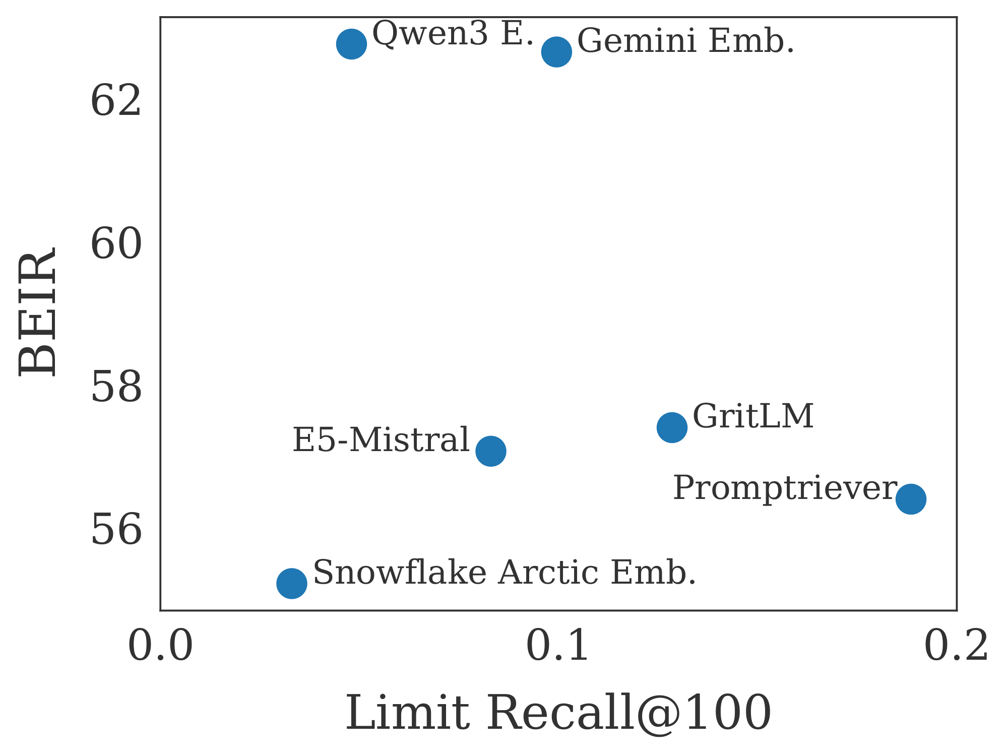
BEIR (used in MTEB v1) ([6, 71]) has frequently been cited as something that embedding models have overfit to ([10, 72]). We compare performance on LIMIT to BEIR in Figure 7. We see that performance is generally not correlated and that smaller models (like Arctic Embed) do worse on both, likely due to embedding dimension and pre-trained model knowledge.

E. LLM Usage

LLMs were not used for any paper writing, only for coding help and title brainstorming.

F. Metrics Measuring Qrel Graph Density

We show two metrics that treat the qrel matrix as a graph and show that LIMIT has unique properties compared to standard IR datasets (Table 2). We call these metrics Graph Density and Average Query Strength and describe them below.

Graph Density

We use the qrel matrix to construct the graph, where nodes are documents and an edge exists between two documents if they are both relevant to at least one common query.

For a given graph $G=(V, E)$ with $V$ being the set of nodes and $E$ being the set of edges, the graph density is defined as the ratio of the number of edges in the graph to the maximum possible number of edges. For an undirected graph, the maximum possible number of edges is $\frac{|V|(|V|-1)}{2}$. Thus, the density $\rho$ is calculated as:

$ \rho = \frac{|E|}{\frac{|V|(|V|-1)}{2}} = \frac{2|E|}{|V|(|V|-1)} $

This metric indicates how connected the graph is; a density of 1 signifies a complete graph (all possible edges exist), while a density close to 0 indicates a sparse graph. For a qrel dataset, the

Average Query Strength

In a query-query graph where nodes are queries and edges represent similarity between queries (e.g., Jaccard similarity of their relevant documents), the strength of a query node $i$, denoted $s_i$, is defined as the sum of the weights of all edges incident to it. If $w_{ij}$ is the weight of the edge between query $i$ and query $j$, and $N(i)$ is the set of neighbors of query $i$, then the strength is:

$ s_i = \sum_{j \in N(i)} w_{ij} $

The Average Query Strength $\bar{s}$ is the mean of these strengths across all query nodes in the graph:

$ \bar{s} = \frac{1}{|V_Q|} \sum_{i \in V_Q} s_i $

where $V_Q$ is the set of all query nodes in the graph. This metric provides an overall measure of how strongly connected queries are to each other on average within the dataset, based on their shared relevant documents.

Comparisons to other datasets

We compare with standard IR Datasets such as NQ ([51]), HotpotQA ([52]), and SciFact ([73]). We also show an instruction-following dataset, FollowIR Core17 ([26]). For all datasets, we use the test set only. The results in Table 2 show that LIMIT has significantly higher values for both of these metrics (i.e. 28 for query similarity compared to 0.6 or lower for the others).

:Table 2: Metrics measuring the density of the qrel matrix. We see that LIMIT is significantly higher than other datasets, but that the closest are instruction-following datasets such as Core17 from FollowIR. Our empirical ablations suggest (although cannot definitively prove) that datasets with higher values here will be harder for retrieval models to represent.

Dataset Name	Graph Density	Average Query Strength
NQ	0	0
HotPotQA	0.000037	0.1104
SciFact	0.001449	0.4222
FollowIR Core17	0.025641	0.5912
LIMIT	0.085481	28.4653

G. Table Forms of Figures

In this section we show the table form of various figures. For Figure 3 it is Figure 3, Figure 4 in Figure 4, Figure 2 in Table 6, and Figure 5 in Figure 5.

::: {caption="Table 3: Fine-tuning results in table form. See Figure 5 for the comparable plot."}

:::

:Table 4: Results for the LIMIT small version. See comparable Figure 4.

Model	Dim	Recall@2	Recall@10	Recall@20
BM25	default	97.8	100.0	100.0
E5-Mistral 7B	32	7.9	32.6	56.2
E5-Mistral 7B	64	10.2	37.0	60.3
E5-Mistral 7B	128	14.5	41.9	65.9
E5-Mistral 7B	256	15.3	45.9	69.7
E5-Mistral 7B	512	22.2	54.7	74.8
E5-Mistral 7B	768	21.6	57.5	79.2
E5-Mistral 7B	1024	24.5	60.5	80.0
E5-Mistral 7B	2048	28.9	66.3	83.2
E5-Mistral 7B	3072	29.9	67.8	85.3
E5-Mistral 7B	4096	29.5	68.1	85.2
GTE-ModernColBERT	default	83.5	97.6	99.1
GritLM 7B	32	7.8	33.5	56.3
GritLM 7B	64	9.4	35.9	59.6
GritLM 7B	128	14.2	42.7	64.9
GritLM 7B	256	17.3	46.2	68.3
GritLM 7B	512	21.8	55.6	76.7
GritLM 7B	768	23.8	58.1	80.1
GritLM 7B	1024	26.2	61.4	80.1
GritLM 7B	2048	33.0	69.1	86.2
GritLM 7B	3072	36.3	72.9	89.9
GritLM 7B	4096	38.4	75.4	90.5
Promptriever Llama3 8B	32	6.1	31.4	56.0
Promptriever Llama3 8B	64	8.9	35.8	62.3
Promptriever Llama3 8B	128	13.7	44.5	67.6
Promptriever Llama3 8B	256	18.5	52.1	74.1
Promptriever Llama3 8B	512	27.0	61.8	81.7
Promptriever Llama3 8B	768	35.5	69.0	84.7
Promptriever Llama3 8B	1024	38.0	73.5	89.1
Promptriever Llama3 8B	2048	46.2	83.6	94.2
Promptriever Llama3 8B	3072	49.2	87.3	96.6
Promptriever Llama3 8B	4096	54.3	90.0	97.7
Qwen3 Embed	32	8.3	30.6	53.9
Qwen3 Embed	64	9.4	35.5	57.6
Qwen3 Embed	128	11.6	38.3	60.8
Qwen3 Embed	256	14.3	41.6	63.8
Qwen3 Embed	512	16.1	43.7	66.0
Qwen3 Embed	768	17.2	45.3	69.3
Qwen3 Embed	1024	17.8	48.7	70.3
Qwen3 Embed	2048	19.5	51.5	72.4
Qwen3 Embed	3072	19.3	52.8	73.3
Qwen3 Embed	4096	19.0	52.3	73.8
Gemini Embed	2	4.2	23.0	45.5
Gemini Embed	4	4.2	21.9	46.0
Gemini Embed	8	4.9	23.2	47.0
Gemini Embed	16	5.2	24.7	47.5
Gemini Embed	32	6.3	25.2	50.6
Gemini Embed	64	6.9	30.6	55.0
Gemini Embed	128	7.7	37.0	62.9
Gemini Embed	256	14.6	46.9	69.7
Gemini Embed	512	23.3	58.4	77.9
Gemini Embed	768	28.8	67.5	84.5
Gemini Embed	1024	31.8	69.9	86.1
Gemini Embed	2048	31.9	70.3	87.1
Gemini Embed	3072	33.7	72.4	87.9
Snowflake Arctic L	32	8.3	30.3	53.8
Snowflake Arctic L	64	9.0	35.4	58.5
Snowflake Arctic L	128	12.7	41.3	65.1
Snowflake Arctic L	256	16.0	48.2	72.6
Snowflake Arctic L	512	16.7	51.3	74.1
Snowflake Arctic L	768	17.9	53.5	74.6
Snowflake Arctic L	1024	19.4	54.9	76.0
Snowflake Arctic L	2048	19.4	54.9	76.0
Snowflake Arctic L	3072	19.4	54.9	76.0
Snowflake Arctic L	4096	19.4	54.9	76.0

:Table 5: Results on LIMIT. See comparable Figure 3.

Model	Dim	Recall@2	Recall@10	Recall@100
E5-Mistral 7B	32	0.0	0.0	0.5
E5-Mistral 7B	64	0.0	0.1	0.4
E5-Mistral 7B	128	0.1	0.3	1.0
E5-Mistral 7B	256	0.4	0.9	1.9
E5-Mistral 7B	512	0.7	1.3	3.8
E5-Mistral 7B	768	0.9	1.7	4.3
E5-Mistral 7B	1024	0.9	1.8	5.9
E5-Mistral 7B	2048	1.0	1.9	6.8
E5-Mistral 7B	3072	1.3	2.0	7.7
E5-Mistral 7B	4096	1.3	2.2	8.3
Snowflake Arctic L	32	0.0	0.1	0.6
Snowflake Arctic L	64	0.2	0.4	1.7
Snowflake Arctic L	128	0.1	0.3	1.8
Snowflake Arctic L	256	0.2	0.8	2.5
Snowflake Arctic L	512	0.3	1.0	2.5
Snowflake Arctic L	768	0.4	1.1	3.1
Snowflake Arctic L	1024	0.4	0.8	3.3
Snowflake Arctic L	2048	0.4	0.8	3.3
Snowflake Arctic L	3072	0.4	0.8	3.3
Snowflake Arctic L	4096	0.4	0.8	3.3
GritLM 7B	32	0.0	0.0	0.8
GritLM 7B	64	0.0	0.1	0.3
GritLM 7B	128	0.1	0.3	1.3
GritLM 7B	256	0.1	0.4	2.8
GritLM 7B	512	0.6	1.8	6.5
GritLM 7B	768	1.5	3.1	8.7
GritLM 7B	1024	1.8	3.5	10.6
GritLM 7B	2048	2.3	4.3	11.8
GritLM 7B	3072	2.0	4.3	12.9
GritLM 7B	4096	2.4	4.1	12.9
Promptriever Llama3 8B	32	0.0	0.0	0.1
Promptriever Llama3 8B	64	0.0	0.0	0.3
Promptriever Llama3 8B	128	0.0	0.1	0.6
Promptriever Llama3 8B	256	0.2	0.4	1.8
Promptriever Llama3 8B	512	0.6	1.4	5.4
Promptriever Llama3 8B	768	1.3	3.1	8.7
Promptriever Llama3 8B	1024	2.1	4.4	12.8
Promptriever Llama3 8B	2048	3.2	6.5	18.1
Promptriever Llama3 8B	3072	2.9	6.3	17.8
Promptriever Llama3 8B	4096	3.0	6.8	18.9
Qwen3 Embed	32	0.0	0.1	1.1
Qwen3 Embed	64	0.0	0.2	1.0
Qwen3 Embed	128	0.3	0.4	1.8
Qwen3 Embed	256	0.4	0.8	3.2
Qwen3 Embed	512	0.6	1.3	3.3
Qwen3 Embed	768	0.7	1.5	3.8
Qwen3 Embed	1024	0.7	1.6	4.6
Qwen3 Embed	2048	0.9	1.7	4.7
Qwen3 Embed	3072	0.8	1.6	4.8
Qwen3 Embed	4096	0.8	1.8	4.8
Gemini Embed	2	0.0	0.0	0.1
Gemini Embed	4	0.0	0.0	0.0
Gemini Embed	8	0.0	0.0	0.0
Gemini Embed	16	0.0	0.0	0.0
Gemini Embed	32	0.0	0.0	0.0
Gemini Embed	64	0.0	0.0	0.3
Gemini Embed	128	0.0	0.1	0.3
Gemini Embed	256	0.0	0.1	1.2
Gemini Embed	512	0.2	1.1	3.6
Gemini Embed	768	0.9	2.5	7.6
Gemini Embed	1024	1.3	2.7	8.1
Gemini Embed	2048	1.5	3.1	8.5
Gemini Embed	3072	1.6	3.5	10.0
GTE-ModernColBERT	default	23.1	34.6	54.8
BM25	default	85.7	90.4	93.6

:Table 6: Critical Values of n for different d values in the Free Embedding optimization experiments. See Figure 2 for the corresponding figure.

$d$	Critical- $n$
4	10
5	14
6	19
7	24
8	28
9	32
10	36
11	42
12	47
13	54
14	62
15	70
16	79
17	89
18	99
19	109
20	120
21	132
22	144
23	157
24	170
25	184
26	198
27	213
28	229
29	245
30	261
31	278
32	296
33	314
34	333
35	352
36	372
37	392
38	413
39	434
40	460
41	484
42	505
43	545
44	605
45	626

:Table 7: BEIR vs LIMIT results. See Figure 7 for the comparable plot.

Model	BEIR	LIMIT R@100
Snowflake Arctic	55.22	3.3
Promptriever	56.40	18.9
E5-Mistral	57.07	8.3
GritLM	57.40	12.9
Gemini Embed	62.65	10.0
Qwen3 Embed	62.76	4.8

References

[1] Stephen E Robertson, Steve Walker, Susan Jones, Micheline M Hancock-Beaulieu, Mike Gatford, et al. Okapi at trec-3. Nist Special Publication Sp, 109:109, 1995.

[2] Kenton Lee, Ming-Wei Chang, and Kristina Toutanova. Latent retrieval for weakly supervised open domain question answering. In Anna Korhonen, David Traum, and Lluís Màrquez (eds.), Proceedings of the 57th Annual Meeting of the Association for Computational Linguistics, pp.\ 6086–6096, Florence, Italy, July 2019. Association for Computational Linguistics. doi:10.18653/v1/P19-1612. URL https://aclanthology.org/P19-1612/.

[3] Nick Craswell, Bhaskar Mitra, Emine Yilmaz, Daniel Campos, and Ellen M Voorhees. Overview of the trec 2019 deep learning track. arXiv preprint arXiv:2003.07820, 2020.

[4] Gautier Izacard, Mathilde Caron, Lucas Hosseini, Sebastian Riedel, Piotr Bojanowski, Armand Joulin, and Edouard Grave. Unsupervised dense information retrieval with contrastive learning. arXiv preprint arXiv:2112.09118, 2021.

[5] Liang Wang, Nan Yang, Xiaolong Huang, Binxing Jiao, Linjun Yang, Daxin Jiang, Rangan Majumder, and Furu Wei. Text embeddings by weakly-supervised contrastive pre-training. arXiv preprint arXiv:2212.03533, 2022.

[6] Nandan Thakur, Nils Reimers, Andreas Rücklé, Abhishek Srivastava, and Iryna Gurevych. Beir: A heterogenous benchmark for zero-shot evaluation of information retrieval models. arXiv preprint arXiv:2104.08663, 2021.

[7] Kenneth Enevoldsen, Isaac Chung, Imene Kerboua, Márton Kardos, Ashwin Mathur, David Stap, Jay Gala, Wissam Siblini, Dominik Krzemiński, Genta Indra Winata, et al. Mmteb: Massive multilingual text embedding benchmark. arXiv preprint arXiv:2502.13595, 2025.

[8] Jinhyuk Lee, Feiyang Chen, Sahil Dua, Daniel Cer, Madhuri Shanbhogue, Iftekhar Naim, Gustavo Hernández Ábrego, Zhe Li, Kaifeng Chen, Henrique Schechter Vera, et al. Gemini embedding: Generalizable embeddings from gemini. arXiv preprint arXiv:2503.07891, 2025.

[9] Orion Weller, Benjamin Chang, Eugene Yang, Mahsa Yarmohammadi, Sam Barham, Sean MacAvaney, Arman Cohan, Luca Soldaini, Benjamin Van Durme, and Dawn Lawrie. mfollowir: a multilingual benchmark for instruction following in retrieval. arXiv preprint arXiv:2501.19264, 2025a.

[10] Orion Weller, Kathryn Ricci, Eugene Yang, Andrew Yates, Dawn Lawrie, and Benjamin Van Durme. Rank1: Test-time compute for reranking in information retrieval. arXiv preprint arXiv:2502.18418, 2025c.

[11] Tingyu Song, Guo Gan, Mingsheng Shang, and Yilun Zhao. Ifir: A comprehensive benchmark for evaluating instruction-following in expert-domain information retrieval. arXiv preprint arXiv:2503.04644, 2025.

[12] Chenghao Xiao, G Thomas Hudson, and Noura Al Moubayed. Rar-b: Reasoning as retrieval benchmark. arXiv preprint arXiv:2404.06347, 2024.

[13] Hongjin Su, Howard Yen, Mengzhou Xia, Weijia Shi, Niklas Muennighoff, Han-yu Wang, Haisu Liu, Quan Shi, Zachary S Siegel, Michael Tang, et al. Bright: A realistic and challenging benchmark for reasoning-intensive retrieval. arXiv preprint arXiv:2407.12883, 2024.

[14] Chaitanya Malaviya, Peter Shaw, Ming-Wei Chang, Kenton Lee, and Kristina Toutanova. Quest: A retrieval dataset of entity-seeking queries with implicit set operations. arXiv preprint arXiv:2305.11694, 2023.

[15] Christos H Papadimitriou and Michael Sipser. Communication complexity. In Proceedings of the fourteenth annual ACM symposium on Theory of computing, pp.\ 196–200, 1982.

[16] Yanzhao Zhang, Mingxin Li, Dingkun Long, Xin Zhang, Huan Lin, Baosong Yang, Pengjun Xie, An Yang, Dayiheng Liu, Junyang Lin, Fei Huang, and Jingren Zhou. Qwen3 embedding: Advancing text embedding and reranking through foundation models. arXiv preprint arXiv:2506.05176, 2025.

[17] Parishad BehnamGhader, Vaibhav Adlakha, Marius Mosbach, Dzmitry Bahdanau, Nicolas Chapados, and Siva Reddy. Llm2vec: Large language models are secretly powerful text encoders. arXiv preprint arXiv:2404.05961, 2024.

[18] Jordan Hoffmann, Sebastian Borgeaud, Arthur Mensch, Elena Buchatskaya, Trevor Cai, Eliza Rutherford, Diego de Las Casas, Lisa Anne Hendricks, Johannes Welbl, Aidan Clark, et al. Training compute-optimal large language models. arXiv preprint arXiv:2203.15556, 2022.

[19] Chunyuan Li, Zhe Gan, Zhengyuan Yang, Jianwei Yang, Linjie Li, Lijuan Wang, Jianfeng Gao, et al. Multimodal foundation models: From specialists to general-purpose assistants. Foundations and Trends® in Computer Graphics and Vision, 16(1-2):1–214, 2024.

[20] Chameleon Team. Chameleon: Mixed-modal early-fusion foundation models. arXiv preprint arXiv:2405.09818, 2024.

[21] Jeffrey Zhou, Tianjian Lu, Swaroop Mishra, Siddhartha Brahma, Sujoy Basu, Yi Luan, Denny Zhou, and Le Hou. Instruction-following evaluation for large language models. arXiv preprint arXiv:2311.07911, 2023.

[22] Long Ouyang, Jeffrey Wu, Xu Jiang, Diogo Almeida, Carroll Wainwright, Pamela Mishkin, Chong Zhang, Sandhini Agarwal, Katarina Slama, Alex Ray, et al. Training language models to follow instructions with human feedback. Advances in neural information processing systems, 35:27730–27744, 2022.

[23] Manuel Faysse, Hugues Sibille, Tony Wu, Bilel Omrani, Gautier Viaud, Céline Hudelot, and Pierre Colombo. Colpali: Efficient document retrieval with vision language models. arXiv preprint arXiv:2407.01449, 2024.

[24] Xueguang Ma, Sheng-Chieh Lin, Minghan Li, Wenhu Chen, and Jimmy Lin. Unifying multimodal retrieval via document screenshot embedding. arXiv preprint arXiv:2406.11251, 2024.

[25] Hongjin Su, Weijia Shi, Jungo Kasai, Yizhong Wang, Yushi Hu, Mari Ostendorf, Wen-tau Yih, Noah A Smith, Luke Zettlemoyer, and Tao Yu. One embedder, any task: Instruction-finetuned text embeddings. arXiv preprint arXiv:2212.09741, 2022.

[26] Orion Weller, Benjamin Chang, Sean MacAvaney, Kyle Lo, Arman Cohan, Benjamin Van Durme, Dawn Lawrie, and Luca Soldaini. Followir: Evaluating and teaching information retrieval models to follow instructions. arXiv preprint arXiv:2403.15246, 2024a.

[27] Niklas Muennighoff, SU Hongjin, Liang Wang, Nan Yang, Furu Wei, Tao Yu, Amanpreet Singh, and Douwe Kiela. Generative representational instruction tuning. In ICLR 2024 Workshop: How Far Are We From AGI, 2024.

[28] Jinhyuk Lee, Zhuyun Dai, Xiaoqi Ren, Blair Chen, Daniel Cer, Jeremy R Cole, Kai Hui, Michael Boratko, Rajvi Kapadia, Wen Ding, et al. Gecko: Versatile text embeddings distilled from large language models. arXiv preprint arXiv:2403.20327, 2024.

[29] Jianqun Zhou, Yuanlei Zheng, Wei Chen, Qianqian Zheng, Zeyuan Shang, Wei Zhang, Rui Meng, and Xiaoyu Shen. Beyond content relevance: Evaluating instruction following in retrieval models. ArXiv, abs/2410.23841, 2024. URL https://api.semanticscholar.org/CorpusID:273707185.

[30] Hanseok Oh, Hyunji Lee, Seonghyeon Ye, Haebin Shin, Hansol Jang, Changwook Jun, and Minjoon Seo. Instructir: A benchmark for instruction following of information retrieval models. arXiv preprint arXiv:2402.14334, 2024.

[31] Orion Weller, Kathryn Ricci, Marc Marone, Antoine Chaffin, Dawn Lawrie, and Benjamin Van Durme. Seq vs seq: An open suite of paired encoders and decoders. arXiv preprint arXiv:2507.11412, 2025b.

[32] Nils Reimers and Iryna Gurevych. The curse of dense low-dimensional information retrieval for large index sizes. arXiv preprint arXiv:2012.14210, 2020.

[33] Aitor Ormazabal, Mikel Artetxe, Gorka Labaka, Aitor Soroa, and Eneko Agirre. Analyzing the limitations of cross-lingual word embedding mappings. arXiv preprint arXiv:1906.05407, 2019.

[34] Zi Yin and Yuanyuan Shen. On the dimensionality of word embedding. Advances in neural information processing systems, 31, 2018.

[35] Georges Voronoi. Nouvelles applications des paramètres continus à la théorie des formes quadratiques. deuxième mémoire. recherches sur les parallélloèdres primitifs. Journal für die reine und angewandte Mathematik (Crelles Journal), 1908(134):198–287, 1908.

[36] Kenneth L Clarkson. Applications of random sampling in computational geometry, ii. In Proceedings of the fourth annual symposium on Computational geometry, pp.\ 1–11, 1988.

[37] Cecilia Bohler, Panagiotis Cheilaris, Rolf Klein, Chih-Hung Liu, Evanthia Papadopoulou, and Maksym Zavershynskyi. On the complexity of higher order abstract voronoi diagrams. Computational Geometry, 48(8):539–551, 2015. ISSN 0925-7721. doi:https://doi.org/10.1016/j.comgeo.2015.04.008. URL https://www.sciencedirect.com/science/article/pii/S0925772115000346.

[38] Der-Tsai Lee. On k-nearest neighbor voronoi diagrams in the plane. IEEE transactions on computers, 100(6):478–487, 1982.

[39] Bi Yu Chen, Huihuang Huang, Hui-Ping Chen, Wenxuan Liu, Xuan-Yan Chen, and Tao Jia. Efficient algorithm for constructing order k voronoi diagrams in road networks. ISPRS International Journal of Geo-Information, 12(4):172, 2023.

[40] Roman Vershynin. High-dimensional probability: An introduction with applications in data science, volume 47. Cambridge university press, 2018.

[41] John H Conway, Chaim Goodman-Strauss, and N Sloane. Recent progress in sphere packing. Current Developments in Mathematics, 1999(1):37–76, 1999.

[42] William B Johnson, Joram Lindenstrauss, et al. Extensions of lipschitz mappings into a hilbert space. Contemporary mathematics, 26(189-206):1, 1984.

[43] Michael J Kearns and Robert E Schapire. Efficient distribution-free learning of probabilistic concepts. Journal of Computer and System Sciences, 48(3):464–497, 1994.

[44] Peter L Bartlett. The sample complexity of pattern classification with neural networks: the size of the weights is more important than the size of the network. IEEE transactions on Information Theory, 44(2):525–536, 2002.

[45] Vladimir Vapnik. Statistical Learning Theory now plays a more active role: after the general analysis of learning processes, the research in the area of synthesis of optimal algorithms was started. These studies, however, do not belong to history yet. They are a subject of today's research activities. PhD thesis, These studies, however, do not belong to history yet. They are a subject of …, 1998.

[46] Aditya Kusupati, Gantavya Bhatt, Aniket Rege, Matthew Wallingford, Aditya Sinha, Vivek Ramanujan, William Howard-Snyder, Kaifeng Chen, Sham Kakade, Prateek Jain, et al. Matryoshka representation learning. Advances in Neural Information Processing Systems, 35:30233–30249, 2022.

[47] Diederik P Kingma and Jimmy Ba. Adam: A method for stochastic optimization. arXiv preprint arXiv:1412.6980, 2014.

[48] Aaron van den Oord, Yazhe Li, and Oriol Vinyals. Representation learning with contrastive predictive coding. arXiv preprint arXiv:1807.03748, 2018.

[49] Kiril Bangachev, Guy Bresler, Iliyas Noman, and Yury Polyanskiy. Global minimizers of sigmoid contrastive loss. arXiv preprint arXiv:2509.18552, 2025.

[50] Jason Wei, Zhiqing Sun, Spencer Papay, Scott McKinney, Jeffrey Han, Isa Fulford, Hyung Won Chung, Alex Tachard Passos, William Fedus, and Amelia Glaese. Browsecomp: A simple yet challenging benchmark for browsing agents. arXiv preprint arXiv:2504.12516, 2025.

[51] Tom Kwiatkowski, Jennimaria Palomaki, Olivia Redfield, Michael Collins, Ankur Parikh, Chris Alberti, Danielle Epstein, Illia Polosukhin, Jacob Devlin, Kenton Lee, et al. Natural questions: a benchmark for question answering research. Transactions of the Association for Computational Linguistics, 7:453–466, 2019.

[52] Zhilin Yang, Peng Qi, Saizheng Zhang, Yoshua Bengio, William W Cohen, Ruslan Salakhutdinov, and Christopher D Manning. Hotpotqa: A dataset for diverse, explainable multi-hop question answering. arXiv preprint arXiv:1809.09600, 2018.

[53] Orion Weller, Benjamin Van Durme, Dawn Lawrie, Ashwin Paranjape, Yuhao Zhang, and Jack Hessel. Promptriever: Instruction-trained retrievers can be prompted like language models. arXiv preprint arXiv:2409.11136, 2024b.

[54] Puxuan Yu, Luke Merrick, Gaurav Nuti, and Daniel Campos. Arctic-embed 2.0: Multilingual retrieval without compromise. arXiv preprint arXiv:2412.04506, 2024.

[55] Liang Wang, Nan Yang, Xiaolong Huang, Linjun Yang, Rangan Majumder, and Furu Wei. Improving text embeddings with large language models. arXiv preprint arXiv:2401.00368, 2023.

[56] Xing Han Lù. Bm25s: Orders of magnitude faster lexical search via eager sparse scoring. arXiv preprint arXiv:2407.03618, 2024.

[57] Antoine Chaffin. Gte-moderncolbert, 2025a. URL https://huggingface.co/lightonai/GTE-ModernColBERT-v1.

[58] Antoine Chaffin and Raphaël Sourty. Pylate: Flexible training and retrieval for late interaction models, 2024. URL https://github.com/lightonai/pylate.

[59] Antoine Chaffin. Modernbert-embed-large, 2025c. URL https://huggingface.co/lightonai/modernbert-embed-large.

[60] Nils Reimers and Iryna Gurevych. Sentence-bert: Sentence embeddings using siamese bert-networks. In Proceedings of the 2019 Conference on Empirical Methods in Natural Language Processing. Association for Computational Linguistics, 11 2019. URL https://arxiv.org/abs/1908.10084.

[61] Gheorghe Comanici, Eric Bieber, Mike Schaekermann, Ice Pasupat, Noveen Sachdeva, Inderjit Dhillon, Marcel Blistein, Ori Ram, Dan Zhang, Evan Rosen, et al. Gemini 2.5: Pushing the frontier with advanced reasoning, multimodality, long context, and next generation agentic capabilities. arXiv preprint arXiv:2507.06261, 2025.

[62] Omar Khattab and Matei Zaharia. Colbert: Efficient and effective passage search via contextualized late interaction over bert. In Proceedings of the 43rd International ACM SIGIR conference on research and development in Information Retrieval, pp.\ 39–48, 2020.

[63] Benjamin Warner, Antoine Chaffin, Benjamin Clavié, Orion Weller, Oskar Hallström, Said Taghadouini, Alexis Gallagher, Raja Biswas, Faisal Ladhak, Tom Aarsen, et al. Smarter, better, faster, longer: A modern bidirectional encoder for fast, memory efficient, and long context finetuning and inference. arXiv preprint arXiv:2412.13663, 2024.

[64] Antoine Chaffin. Reason-moderncolbert, 2025b. URL https://huggingface.co/lightonai/Reason-ModernColBERT.

[65] Julian Killingback, Hansi Zeng, and Hamed Zamani. Hypencoder: Hypernetworks for information retrieval. In Proceedings of the 48th International ACM SIGIR Conference on Research and Development in Information Retrieval, pp.\ 2372–2383, 2025.

[66] Shai Ben-David, Nadav Eiron, and Hans Ulrich Simon. Limitations of learning via embeddings in euclidean half spaces. Journal of Machine Learning Research, 3(Nov):441–461, 2002.

[67] Andreas Grivas, Antonio Vergari, and Adam Lopez. Taming the sigmoid bottleneck: Provably argmaxable sparse multi-label classification. In Proceedings of the AAAI Conference on Artificial Intelligence, volume 38, pp.\ 12208–12216, 2024.

[68] Samy Badreddine, Emile van Krieken, and Luciano Serafini. Breaking rank bottlenecks in knowledge graph embeddings. arXiv preprint arXiv:2506.22271, 2025.

[69] Rohan Paul, Haw-Shiuan Chang, and Andrew McCallum. Multi-facet universal schema. In Proceedings of the 16th Conference of the European Chapter of the Association for Computational Linguistics: Main Volume, pp.\ 909–919, 2021.

[70] Noga Alon, Peter Frankl, and Vojtech Rodl. Geometrical realization of set systems and probabilistic communication complexity. In 26th Annual Symposium on Foundations of Computer Science (sfcs 1985), pp.\ 277–280. IEEE, 1985.

[71] Niklas Muennighoff, Nouamane Tazi, Lo"ıc Magne, and Nils Reimers. Mteb: Massive text embedding benchmark. arXiv preprint arXiv:2210.07316, 2022.

[72] Nandan Thakur, Jimmy Lin, Sam Havens, Michael Carbin, Omar Khattab, and Andrew Drozdov. Freshstack: Building realistic benchmarks for evaluating retrieval on technical documents. arXiv preprint arXiv:2504.13128, 2025.

[73] David Wadden, Shanchuan Lin, Kyle Lo, Lucy Lu Wang, Madeleine van Zuylen, Arman Cohan, and Hannaneh Hajishirzi. Fact or fiction: Verifying scientific claims. arXiv preprint arXiv:2004.14974, 2020.