LeRoPE: Learnable RoPE Frequencies Improve Language Modeling

Petros Karypis$^{*}$
UC San Diego

Sean O'Brien$^{*}$
UC San Diego

Shreyas Kadekodi
UC San Diego

Rui Zhu
Independent Researcher

Julian McAuley
UC San Diego

$^{*}$ Primary authors. Correspondence: [email protected]

Abstract

Rotary Positional Encodings (RoPE) are currently the most popular positional encodings used in modern language models. RoPE rotates two-dimensional chunks of query and key vectors, operating as a function of their relative positional offset. The position-wise rates of rotation in RoPE typically follow a geometric sequence specified by a fixed base-frequency hyperparameter. Prior work has improved performance by either increasing this parameter to slow rotation or by applying RoPE to only a subset of QK dimensions. In this work we modify RoPE by learning a scalar per frequency, treating frequencies as learnable parameters rather than hyperparameters. We validate Learned RoPE by training a ladder of language models from scratch, ranging from 52M to 2.5B parameters. We observe and analyze the emergence of a high-norm, positional LeRoPE band. LeRoPE consistently outperforms RoPE and partial RoPE across all scales, with RoPE requiring 3.4% more compute (FLOPs) to match LeRoPE at the largest scale.

Executive Summary: Executive Summary

Modern decoder-only language models rely on Rotary Positional Encodings (RoPE) to supply relative position information because self-attention itself is position-agnostic. The rotation rates in standard RoPE are fixed by a single base-frequency hyperparameter; recent analyses show that the slowest bands contribute little positional signal and can be removed or slowed with modest gains. The present work asks whether those rates can be improved further by making them learnable parameters rather than fixed hyperparameters.

The authors introduce Learned RoPE (LeRoPE), which adds one scalar multiplier per frequency band—only 32 extra parameters for the models studied—and trains them jointly with the rest of the network. They evaluate the method on a compute-optimal scaling ladder of decoder-only Transformers (52 M to 2.5 B parameters) trained on the C4 corpus for 20N tokens, comparing against both standard RoPE (base 10 000) and Partial RoPE (p-RoPE, p = 0.75).

Across every scale LeRoPE reaches lower validation perplexity than the two baselines. At the 2.5 B scale the gap corresponds to a 3.4 % compute multiplier: standard RoPE would require 3.4 % more FLOPs to match LeRoPE performance. The advantage grows with sequence length, and LeRoPE also improves in-distribution needle-in-a-haystack retrieval. Analysis of the trained models reveals a consistent frequency profile: fast bands remain near their RoPE-initialized values while the slowest bands are driven toward zero; a single “dominant positional band” emerges at a wavelength of roughly 2.2 × the training length and carries most of the positional contribution to attention logits. Freezing the learned frequencies after a separate run captures about 63 % of the full gain, while p-RoPE captures only ~10 %.

These results indicate that jointly optimizing the rotation rates yields a small but reliable efficiency improvement without changing model architecture or training recipe. The method is compatible with existing context-extension techniques such as YaRN, and the learned frequencies transfer across random seeds and scales. At current frontier training budgets a 3 % compute saving is material; practitioners should therefore consider adopting LeRoPE (or at minimum transferring its learned frequencies) for new pre-training runs. Further validation at >10 B parameters and on heavily over-trained regimes remains necessary before the finding can be treated as definitive.

1. Introduction

Section Summary: Transformers need explicit positional signals because self-attention does not encode token order on its own. Rotary positional encodings achieve this by rotating pairs of query and key vectors at different fixed frequencies so that their dot product reflects only the distance between tokens. The authors show that replacing these fixed frequencies with a small set of learned values yields consistent gains across model sizes and reduces the compute needed to reach a given performance level.

Positional encodings are typically included in Transformer-based models ([1]) because the self-attention operation on its own does not directly carry positional signal. Rotary Positional Encodings (RoPE) ([2]) are used by a number of popular language models ([3, 4, 5, 6]). RoPE splits the query and key vectors into two-dimensional pairs, or frequency bands, and rotates each pair by an angle proportional to token position. The effect of these rotations on the query–key inner product depends only on the relative offset between tokens. Each band rotates at its own fixed rate, following a geometric sequence set by a base hyperparameter: high-frequency bands complete many rotations within a context, while the lowest-frequency bands rotate minimally.

The choice of these frequencies matters. Recent work finds that the slowest bands carry semantic rather than positional information ([7]). This positional invariance allows content matches to hold at any separation, making it beneficial to remove rotation from a subset of bands entirely, or to adjust the base, which sets how many bands rotate appreciably within the context window ([7, 8, 9]).

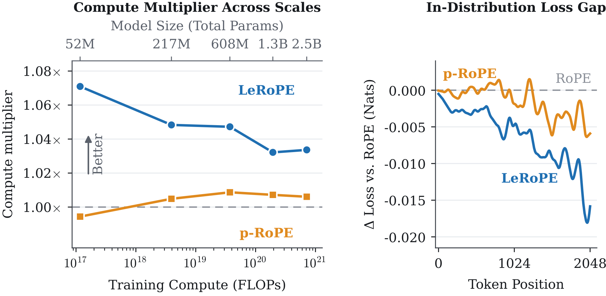
Motivated by the above, and noting that the RoPE operation is differentiable with respect to its frequency, we propose learning the frequencies. Learned RoPE (LeRoPE) adds one learned scalar per frequency band, 32 parameters in total for each of our models. Training on a ladder of models from 52M to 2.5B parameters, LeRoPE outperforms RoPE at every scale. At the largest scale, RoPE requires $3.4%$ more compute to match the performance of LeRoPE (Figure 1).

Analyzing models trained with LeRoPE, we observe a consistent frequency profile across scales and random seeds, as well as the emergence of a single band with a large, strongly positional contribution to the attention logits, which we term the "dominant positional band."

2. Preliminaries

Section Summary: Positional embeddings were introduced to give attention-based language models a sense of token order, evolving from fixed or learned absolute offsets to relative methods such as rotary positional embeddings (RoPE). RoPE rotates pairs of dimensions in the query and key vectors at different frequencies so that their dot product naturally encodes only the relative distance between tokens rather than their absolute positions. Later work observed that the slowest-rotating frequency bands mainly carry semantic information and showed that freezing or removing them—via techniques like partial RoPE—can improve length generalization without harming performance.

2.1 Positional Embeddings

To break the positional symmetry of the attention mechanism, [1] add fixed sinusoidal positional embeddings directly to the input residual stream. Later models instead incorporated learned absolute positional embeddings ([10, 11, 12, 13, 14]).

[15] proposed relative position representations, which depend only on the relative offset between tokens; a simplified, scalar version of learned relative offsets was adopted by T5 ([16]). Rotary positional embeddings, proposed by [2], also depend only on relative position, and have become the standard choice for modern language models.

Since RoPE, a number of positional encodings have been proposed. ALiBi ([17]) improved out-of-distribution length extrapolation with fixed relative positional biases. CoPE provides the model with the capacity to produce relative positional embeddings from learned, content-dependent features ([18]); PaTH also proposes a data-dependent relative transform based on accumulating Householder matrices ([19]).

Some methods generalize to a broader class of functions, of which RoPE is a member. For instance, LieRE learns skew-symmetric matrices that can rotate along planes other than the standard RoPE plane ([20]). [21] generalize RoPE to a broader class of wavelet-function-based positional encodings, finding improved performance from Ricker-based wavelets.

2.2 RoPE

[2] propose Rotary Position Embedding (RoPE), a relative positional embedding method that forms the basis of our study. RoPE rotates key and query vectors according to their position, modifying their inner product according only to their relative offset.

Concretely, consider a single attention head with per-head dimension $d_h$. The dimensions of this head can be chunked into $d_h/2$ frequency pairs, indexed by $m = 0, \ldots, d_h/2-1$. Standard RoPE assigns each pair a frequency from a geometric series:

$ \theta_m = b^{-2m/d_h}, \quad m = 0, \ldots, d_h/2-1,\tag{1} $

where $b > 1$ is the base (typically $b = 10{,}000$). Following the notation of [7] we denote $\rho(\theta_m)$ as the matrix form of the rotational transformation of angle $\theta_m$:

$ \rho(\theta_m) = \begin{bmatrix} \cos(\theta_m) & -\sin(\theta_m) \ \sin(\theta_m) & \cos(\theta_m) \end{bmatrix}\tag{2} $

RoPE constructs a block-diagonal matrix $\textbf{R}s = {\oplus}{m=0...d_h /2-1} \rho (\theta^{(m)})^s$ where $s$ is the position of a given token. It then applies $\textbf{R}_s$ to each key and query vector; that is $\tilde{q}_s = \textbf{R}_s q_s$ and $\tilde{k}_s = \textbf{R}_s k_s$.

The rotation-matrix properties $\rho(\theta)\rho(\theta') = \rho(\theta + \theta')$ as well as $\rho(\theta)^\intercal = \rho(-\theta)$, in conjunction with the block-diagonal structure of $\textbf{R}_s$ gives the relation $\textbf{R}_s^\intercal \textbf{R}t = \textbf{R}{t - s}$. The dot product of a RoPE-rotated query-key pair $\tilde{q}_s, \tilde{k}_t$ decomposes into:

$ \tilde{q}_s^\intercal \tilde{k}_t^{\vphantom{\intercal}} = (\textbf{R}s q_s)^\intercal (\textbf{R}t k_t) = q_s^\intercal \textbf{R}{t-s}k_t = \sum{m=0...d_h/2-1} \left(q_s^{(m)} \right)^T \rho(\theta_m)^{t-s} k_t^{(m)}\tag{3} $

where $q_s^{(m)}$ is the 2 dimensional chunk (or band) of the query vector $q_s^{[2m, 2m+1]}$ (the same notation holds for the key vectors). Thus, the RoPE operation depends only on the relative offset $t - s $ and not on the absolute positions $s$ and $t$.

2.3 Frequency Bands and Partial RoPE

Each index $m$ in Equation 1 defines a frequency band: a two-dimensional sub-vector rotated at angular frequency $\theta_m$, completing a full period every $2\pi/\theta_m$ tokens. Because the frequencies are geometrically spaced, these periods span several orders of magnitude, and the slowest bands typically do not complete a single period within the training context.

Trained models do not use this spectrum uniformly. [7] show that RoPE models concentrate query and key norm in the lowest-frequency bands and argue that these bands, which rotate negligibly over typical offsets, transport semantic rather than positional information. Since even a slow band eventually drifts over long ranges, they propose Partial RoPE ($p$-RoPE), which removes rotation from the slowest bands entirely:

$ \theta_m = \begin{cases} b^{-2m/d_h} & m < p \cdot d_h/2, \ 0 & \text{otherwise}, \end{cases}\tag{4} $

where $p$ is the fraction of bands kept. Setting $p{=}1$ recovers RoPE, while $p{=}0$ recovers NoPE — omitting positional encoding altogether — which itself improves length generalization ([22]). Adjusting the base $b$ acts on the same lever continuously: raising it slows every band rather than zeroing the slowest, and is an effective tool for context extension ([23, 8]), adopted at scale in recent open models ([6]).

[9] expand this analysis and identify a contiguous high-norm band of RoPE dimensions that emerges early in pre-training, with its location determined jointly by the base $b$ and the training length. Lower frequency bands can be replaced with NoPE at inference at little cost, confirming that the slowest frequencies are only weakly used for position. All of these methods, however, fix the band allocation by hand before training.

3. LeRoPE

Section Summary: LeRoPE modifies rotary position embeddings by introducing one learned scaling factor per frequency band that multiplicatively adjusts rotation speeds while sharing these factors across all layers and heads. The scalars begin at zero so training starts identically to standard RoPE, use logarithmic parametrization for stable updates, and receive special optimization handling such as no weight decay and separate gradient clipping. The section further shows that each frequency evolves according to the derivative of a surrogate loss equivalent to the real part of a discrete Fourier transform of offset-aggregated attention gradients.

3.1 Extending RoPE to Learned Frequencies

LeRoPE augments RoPE with one learned scalar $\alpha_m$ per frequency band, rescaling each frequency:

$ \hat\theta^{(m)} = e^{\alpha_m}\theta^{(m)}, \qquad \mathbf{R}^{\mathrm{LeRoPE}}s = \bigoplus{m=0}^{d_h/2-1} \rho\big(\hat\theta^{(m)}\big)^{s}.\tag{5} $

We parametrize frequency scalars in logarithmic space, so that steps in $\alpha_m$ make multiplicative changes to $\hat\theta^{(m)}$. This yields better conditioning when scaling down frequencies and avoids undesirable gradient dynamics near frequencies of zero. We initialize $\alpha_m = 0$, making our method equivalent to RoPE on initialization. Additionally, we omit weight decay on LeRoPE parameters, and apply gradient clipping to them independently of the rest of the model's parameters.

All layers and heads share the same set of learned frequencies; thus, with $d_h$ as the head dimension, LeRoPE adds $d_h/2$ total parameters to the model. The parametrization also admits finer granularity (e.g., per-layer or per-head), but we find that sharing $\alpha_m$ values across all layers and heads performs consistently best.

3.2 Gradient of a Frequency

Each learned frequency receives its gradient through the per-band contributions of Equation 3. Writing the band- $m$ chunks in polar form and differentiating,

$ \begin{aligned} \frac{\partial \mathcal{L}}{\partial \hat\theta^{(m)}} &= -\sum_{s}\sum_{t < s} (s-t), \big|q_s^{(m)}\big|, \big|k_t^{(m)}\big|, \sin!\big(\phi^{(m)}{st} + (s-t), \hat\theta^{(m)}\big), \frac{\partial \mathcal{L}}{\partial z{st}} \end{aligned}\tag{6} $

where $\phi^{(m)}{st}$ is the angle from the key to the query chunk and $z{st}$ the attention logit.

We can express the gradient update as the derivative of a surrogate loss $P(\theta)$. Let $\alpha_{st}$ be the post-softmax attention weight from query $q_s$ to key $k_t$; let $v_t$ be the value vector at position $t$ and $o_s = \sum_{t < s} \alpha_{st} v_t$ be the attention-aggregated output vector, before projection for simplicity. Further, let $g_s \triangleq \partial \mathcal{L} / \partial o_s$ be the downstream gradient and $L$ the maximum context length.

With these quantities, we can define a spectral function of offset $C_m(\delta)$. The direction of each term is dictated by the relative QK angle $\phi_{st}^{(m)}$, and its scale is the product of QK norms, post-softmax probability, and the downstream gradient term.

$ \begin{aligned} C_m(\delta) &\triangleq \sum_{\substack{s, t \s-t=\delta}} \alpha_{st} |q_s^{(m)} | |k_t^{(m)}| e^{i\phi_{st}^{(m)}} (v_t - o_s)^T g_s = R_m (\delta) e^{i\Phi_m(\delta)} \ P_m(\theta) &= \text{Re}\left(\sum_{\delta=1}^{L-1} C_m(\delta) e^{i \delta \theta} \right) = \sum_{\delta=1}^{L-1} R_m(\delta) \cos \left(\Phi_m(\delta) + \delta \theta \right) \end{aligned} $

########## {caption="Lemma 1"}

Define $P_m(\theta)$ as above: the real component of the discrete-time Fourier Transform of the offset-aggregated gradient signal $C_m(\delta)$ with frequency $\theta$.

Then $\frac{\partial \mathcal{L}}{\partial \theta^{(m)}} = P_m'\left(\theta^{(m)}\right)$.

Proof: See Lemma 3.

This provides one perspective on how $\theta^{(m)}$ is updated. Each offset $\delta$ is mapped to a complex phasor $C_m(\delta)$, which aggregates the downstream gradients weighted by QK norms, un-rotated QK relative angles, and the post-softmax attention weights $\alpha_{st}$.

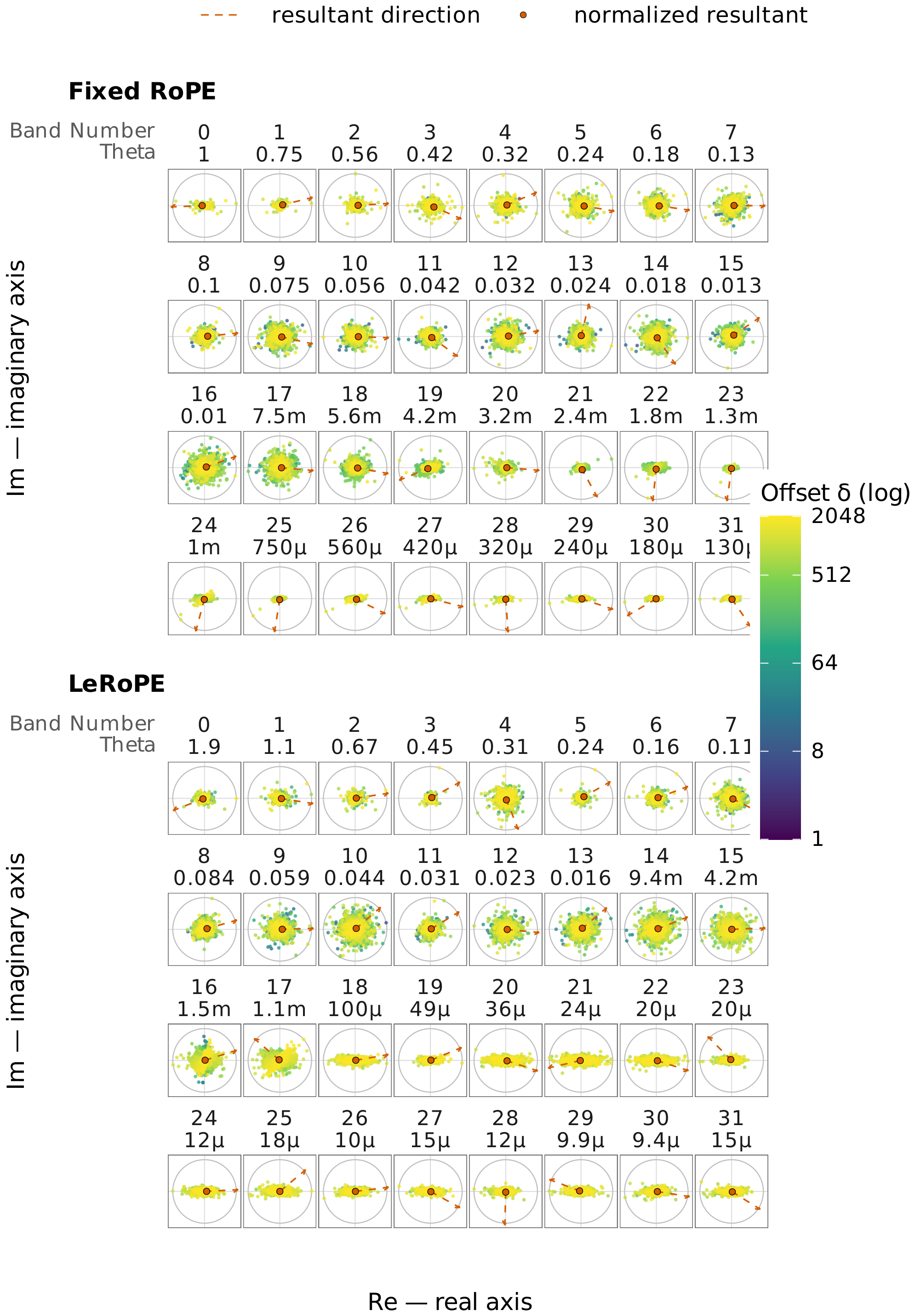
Then, $\theta^{(m)}$ is updated towards the local minimum of the surrogate function $P_m(\theta)$, which is the real component of the discrete-time Fourier Transform of the series, evaluated at frequency $\theta$. The effect of each relative offset on this gradient can be characterized by visualizing the per-offset phasors $C_m(\delta)$: we plot these for each band in Appendix B.2 to illustrate the per-offset geometries; the phasors largely cancel about the origin rather than cohering.

4. Experimental Setup

Section Summary: In this experimental setup, researchers trained a range of decoder-only transformer models from 52 million to 2.5 billion parameters on the C4 dataset, scaling both model size and training tokens together under compute-optimal conditions with a fixed sequence length of 2048. They compared their proposed LeRoPE method against standard RoPE and a variant called p-RoPE, carefully tuning learning rates at each scale to ensure fair evaluation while keeping other architectural details consistent. To quantify efficiency gains, they introduced "compute multipliers," which measure how much less training compute LeRoPE requires to match the validation loss achieved by the baseline RoPE through interpolated loss-versus-compute curves.

\begin{tabular}{lccccc}
  \toprule
  Method & 52M & 217M & 608M & 1.34B & 2.52B \\
  \midrule
  RoPE & 30.2450 & 18.2377 & 13.8795 & 11.5747 & 10.1720 \\
  $p$-RoPE & 30.2695 & 18.2269 & 13.8663 & 11.5665 & 10.1659 \\
  \midrule
  LeRoPE & \textbf{29.9479} & \textbf{18.1335} & \textbf{13.8093} & \textbf{11.5384} & \textbf{10.1387} \\
  \bottomrule
  \end{tabular}

4.1 Scaling Ladder

To evaluate our proposed method we train a family of decoder-only transformers ranging in size from $52\text{M}$ to $2.5\text{B}$ parameters under a compute-optimal regime. Following previous works ([24, 25]) we co-scale layers and head count keeping the head dimension fixed at 64 so all models have the same number of learned frequency scales. We adopt the Chinchilla token count of $D = 20N$ where $N$ is the total number of model parameters. We use C4 ([16]) as our pre-training corpus and a sequence length of 2048 with intra-document masking. During evaluation we do not pack documents. An exhaustive overview of our architecture, hyper-parameters and differences from existing works can be found in Appendix A.1.

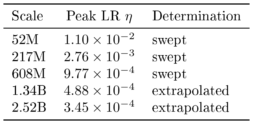
We compare against RoPE with the standard base $b=10{,}000$ and $p$-RoPE with $p=0.75$ following [7]. For every model below 1.34B parameters we sweep the learning rate over a geometric grid, $\eta \in {2^{-i/2} : i \in \mathbb{Z}}$, until the best value is bracketed by a tested value on either side. We run this sweep independently for each of the three positional-encoding methods, and find that all three share the same optimal learning rate at every scale; comparisons at a given scale therefore use identical hyperparameters. For the two largest models we extrapolate the best grid index from the smaller scales.

4.2 Compute Multipliers

To evaluate the benefit of a proposed architecture change, an important quantity to measure is the amount of compute saved relative to the baseline in order to reach the same performance. We report this through compute multipliers: a compute multiplier of $1.x$ for LeRoPE corresponds to needing $x% more compute to reach the same loss with RoPE.

We measure the training compute of each model as $C = 6 ND$ FLOPs, where $N$ is its number of non-embedding parameters. For each method we form a loss–compute curve by piecewise-linear interpolation of the final validation losses of its compute-optimal models in $(\log C, L)$ space and extrapolating beyond the smallest and largest scales with the slope of the nearest segment. Writing $L^{\mathrm{RoPE}}$ and $L^{\mathrm{var}}$ for the baseline and variant curves, the compute multiplier of a variant trained at compute $C^{\mathrm{var}}$ is

$ \mathrm{CM} ;=; \frac{C^{\mathrm{RoPE}}}{C^{\mathrm{var}}}, \qquad\text{where}\qquad L^{\mathrm{RoPE}}!\big(C^{\mathrm{RoPE}}\big) = L^{\mathrm{var}}!\big(C^{\mathrm{var}}\big),\tag{7} $

i.e. the factor by which RoPE's compute must increase to reach the variant's loss, obtained by inverting the interpolated $L^{\mathrm{RoPE}}$.

Our scaling ladder is sparser than that of [24], with adjacent scales differing by a decade or more of compute. Linear interpolation across these gaps overestimates the multiplier for the convex power-law loss curve, so we invert Equation 7 in $\log C$ rather than $C$ to reduce the overestimation. We include further discussion on this choice as well as a comparison with the more traditional efficiency gain fitted power-law inversion method ([26]) in Appendix A.2.

5. Results

Section Summary: Experiments show that LeRoPE delivers modestly lower validation perplexity than standard RoPE or its partial variant across model scales, an advantage equivalent to RoPE needing roughly 3.4 percent more compute to match performance, with the gap widening at longer contexts. Variability checks across random seeds confirm the improvement is reliable rather than due to chance. In needle-in-a-haystack retrieval tests with multiple distractors placed inside the training length, LeRoPE also sustains higher accuracy than the baselines.

: Table 2: Validation perplexity and percentage of LeRoPE gain captured by each method on a 217M-parameter model. Fixed LeRoPE uses frozen frequencies learned by LeRoPE on a separate run at the same scale.

Method	Perplexity	% Gain Captured
RoPE	18.2377	0%
$p$-RoPE	18.2269	10.4%
Fixed LeRoPE	18.1714	63.6%
LeRoPE	18.1335	100%

needspace15baselineskip

5.1 Compute Multipliers

We report the compute multipliers for LeRoPE and $p$-RoPE in Figure 1(a), and the corresponding validation perplexity numbers in Table 1. Across all scales LeRoPE realizes a small but consistent gain, corresponding to RoPE requiring $3.4%$ more compute to match it at the largest scale. We also include the loss delta relative to RoPE as a function of position in Figure 1 (b). LeRoPE's gain over RoPE grows with context length, suggesting it makes better use of longer context.

To bound run-to-run variability, we repeat the 217M RoPE and LeRoPE runs with three random seeds. The method gap of $0.0066$ nats is $3$ to $7$ times the per-method seed standard deviation; LeRoPE improves on RoPE under every seed, with the worst LeRoPE run outperforming the best RoPE run by $0.0034$ nats. The exact numbers as well as additional ablations, including per-head per-layer experiments, can be found in Appendix C.

5.2 In-Distribution Needle-in-a-Haystack

Needle in a Haystack (NIAH) is a standard probe of context utilization and retrieval: given a key, the model must retrieve its associated value from a context of filler text and, optionally, distractor key–value pairs. Examples are generated synthetically; we vary the depth of the gold pair (the "needle") within the context, using filler text from the original NIAH repository.^1

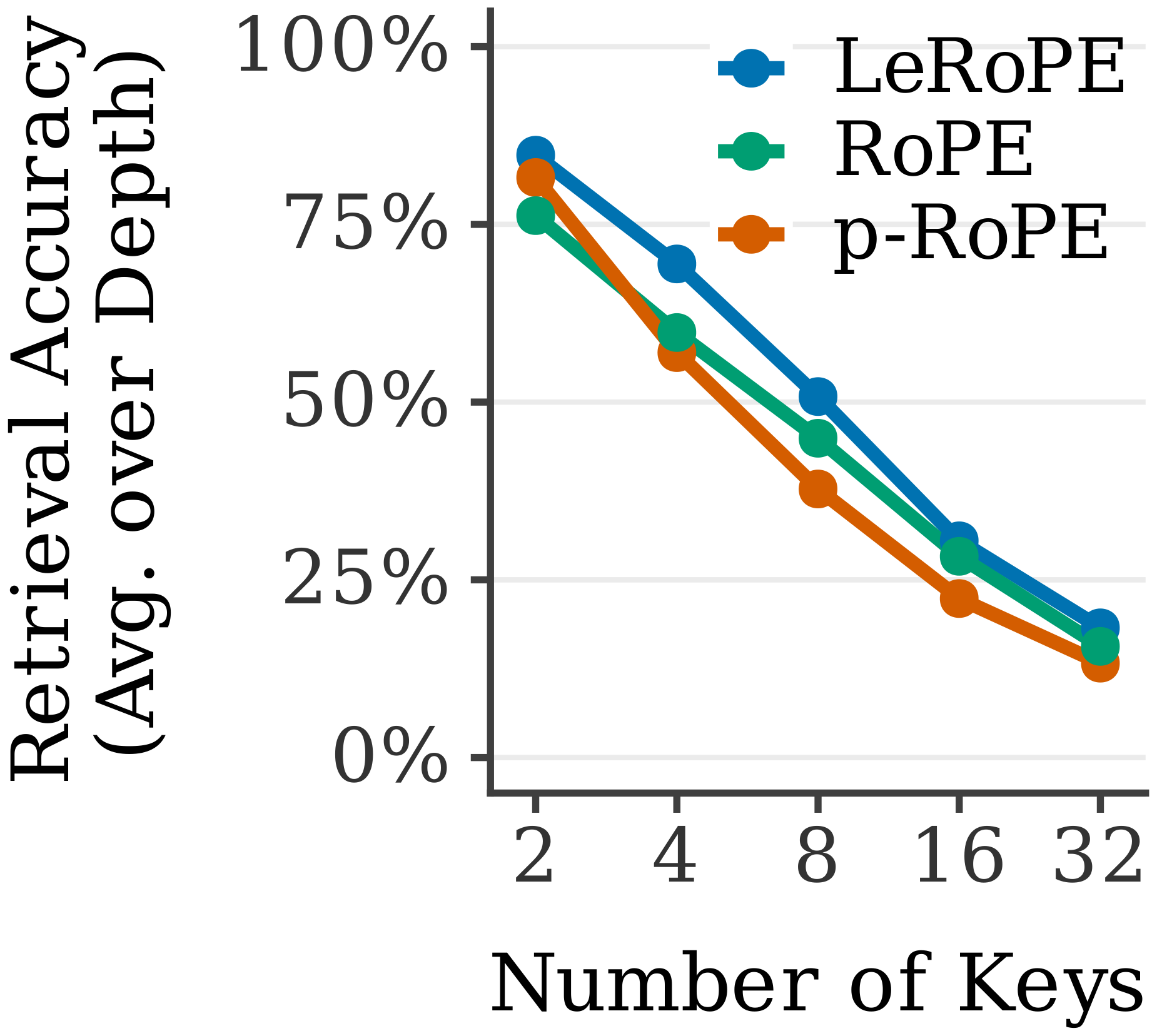
We evaluate the 2.5B models with 1 to 31 distractor pairs across all three methods placing the needle at depths ${0, 0.1, \ldots, 1.0} \times L_{\text{train}}$. Figure 2 plots retrieval accuracy against distractor count, averaged over depths: LeRoPE outperforms RoPE and $p$-RoPE at every shared count, and continues to outperform RoPE at 31 distractor pairs, the hardest setting evaluated. All evaluations here stay within $L_{\text{train}}$, as this section targets in-distribution behavior; we report only the multi-key variant because single-needle retrieval is saturated for all models in-distribution, and we defer length extrapolation to Section 7.

Section Summary: LeRoPE is $3.4%$ more compute efficient than RoPE, leading to a final model with better in-distribution performance for a fixed compute budget.

6. Analysis: Learned Frequency Patterns

Section Summary: LeRoPE modifies standard rotational position encodings by learning a set of frequencies tailored to the training data. Across model sizes and random seeds, it consistently suppresses the slowest frequencies whose wavelengths exceed the training length, leaving a single dominant band whose wavelength settles at roughly 2.2 times that length. Freezing the network to these discovered frequencies recovers about 63 percent of LeRoPE’s total gains, showing that both the final frequency values and the joint training process contribute to the improvement.

We now study what LeRoPE learns. We examine the learned frequencies directly and identify a single band that carries most of the positional signal.

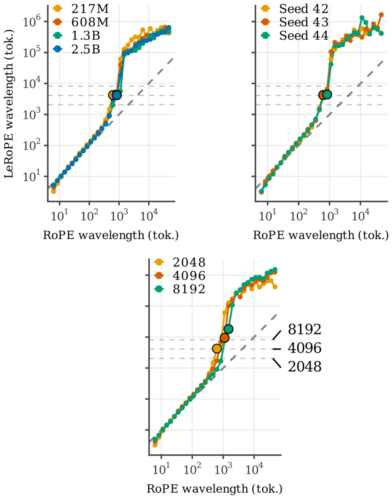
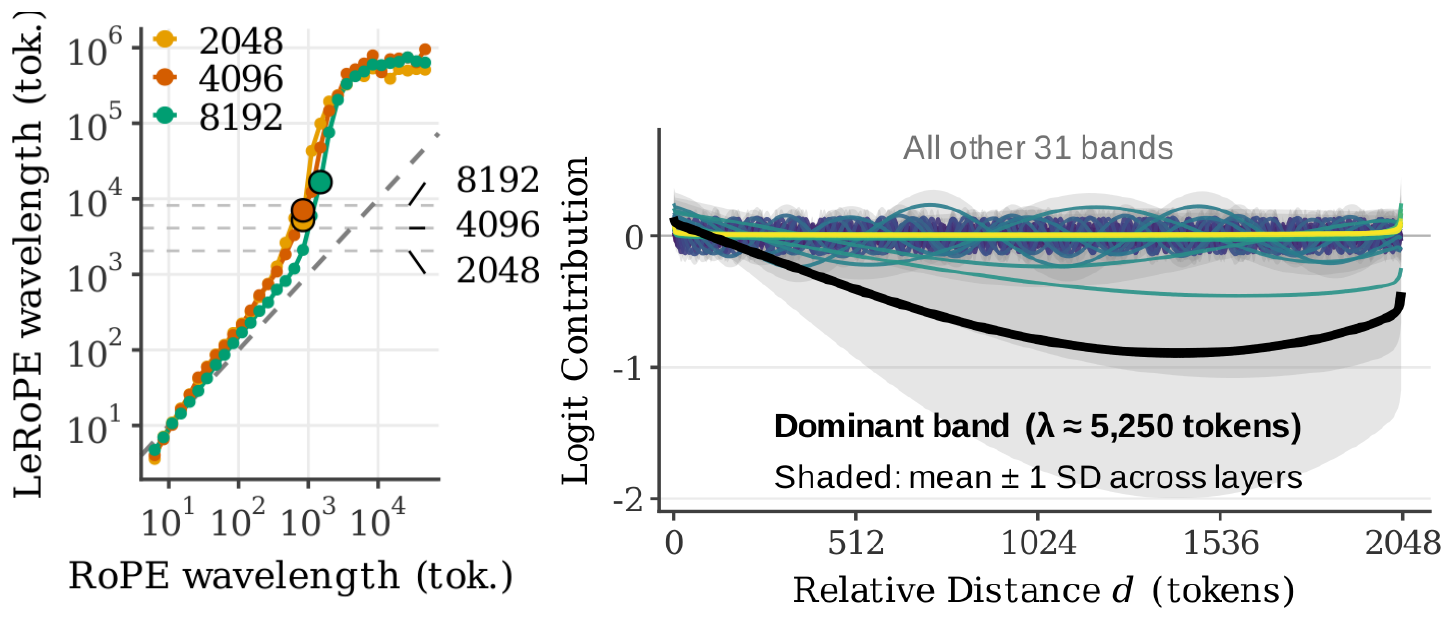
Learned Frequencies. Figure 3 plots each learned band's wavelength against RoPE's counterpart: low-wavelength bands closely track RoPE ($y=x$), mid-wavelength bands begin to diverge, and high-wavelength bands are pushed to a much larger, near-constant wavelength – i.e. their frequency is driven toward zero. High-frequency (low-wavelength) bands rotate slightly faster, with the effect more pronounced for smaller scales. Mid-frequency bands begin to slow compared to RoPE frequencies, and low frequencies are driven down even closer to zero. This pattern is consistent across all model scales and seeds we test (Figure 3 a, b).

The point at which frequencies are suppressed is linked to the sequence lengths seen during training (Figure 3 c): models trained on longer contexts diverge from the RoPE frequencies at lower frequencies than their short-context counterparts.

Identifying Dominant Positional Bands. Equation 3 provides a per-band decomposition of the attention logit contributions. By plotting the average contribution per relative distance, we find (Figure 4) that one band dominates in a nearly purely positional pattern for models with LeRoPE.

The dominant band's wavelength tracks the training length across six runs: four model scales at $L_{\text{train}}=2048$, plus 217M runs at $L_{\text{train}}\in{4096, 8192}$. The dominant band's wavelength is $\approx 2.205, L_{\text{train}}$ (exact wavelengths can be in Table 10). Fixed-frequency RoPE models trained at the same scale do not exhibit a dominant band. Instead, their positional contributions are distributed across several bands at far smaller magnitudes, although, as noted by [21], they do contain strongly oscillatory channels.

Learning With Fixed LeRoPE Frequencies. Next, we ask whether the improvements from LeRoPE emerge from jointly training frequencies with the rest of the network, or solely from the discovery of a more optimal set of frequencies. To distinguish these, we train a 217M model with its frequencies frozen to the values learned by an independent LeRoPE run at the same scale (Table 2).

Training with fixed LeRoPE frequencies yields 63% of the improvement of full LeRoPE, suggesting that joint training dynamics and the final frequency set are both partially responsible for performance gains. Under the same settings, $p$-RoPE captures $10.4%$ of the performance gains of LeRoPE. We can interpret $p$-RoPE as a coarse approximation of final LeRoPE frequencies, preserving faster frequencies while suppressing slower ones.

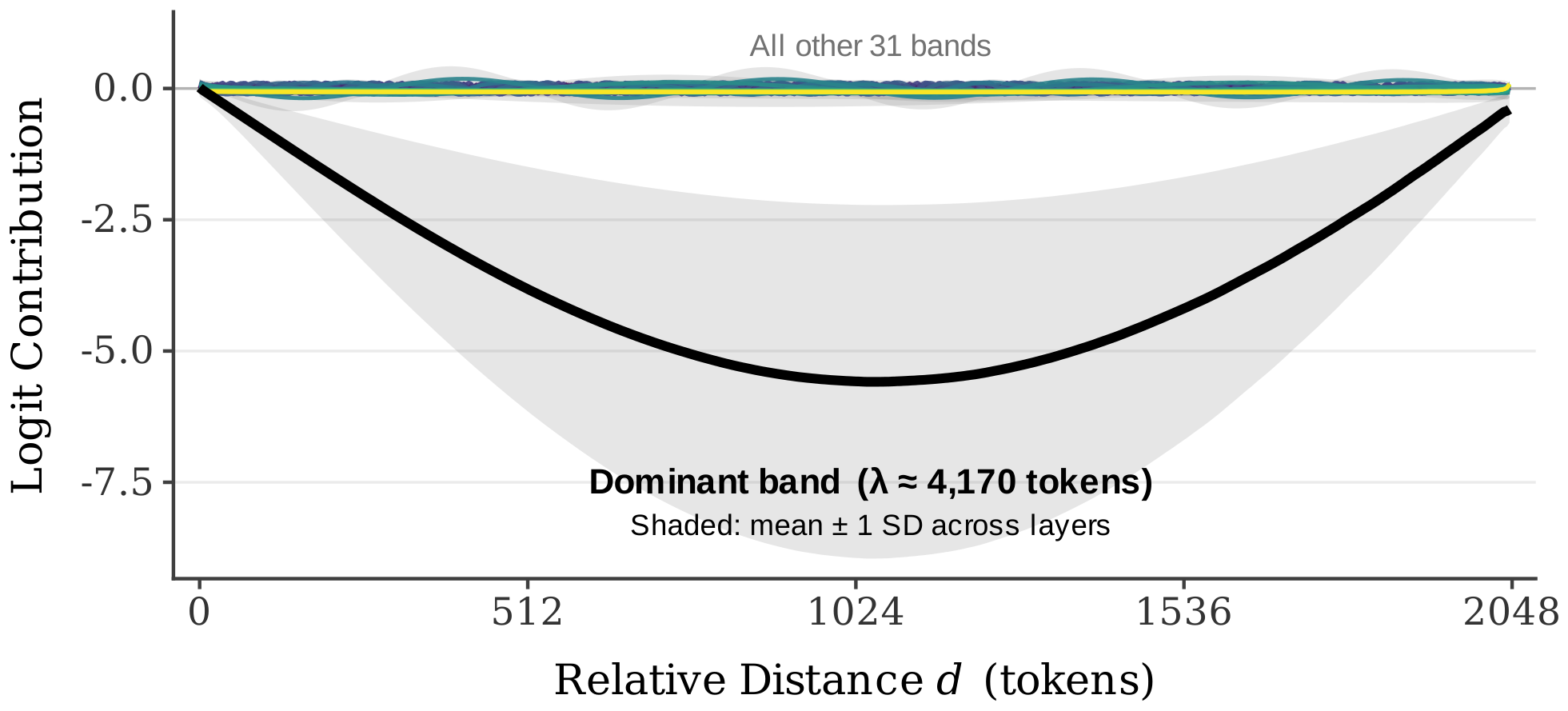
Section Summary: *LeRoPE learns the same frequency profile across seeds and scales: frequencies too slow for the training window are suppressed, and a single dominant band emerges at $\lambda \approx 2.2, L_{train}$.

Training with the learned frequencies frozen captures $63.6%$ of the gain.*

7. Extrapolation

Section Summary: LeRoPE degrades more sharply than standard RoPE when sequences exceed the training length, because its dominant frequency band shifts from a near-zero or negative contribution to a positive one on unseen distances. Targeted interpolation on just that band, or pairing LeRoPE with established scaling tools such as NTK-by-parts and YaRN, largely prevents the sudden rise in perplexity and yields stronger results than the same methods applied to RoPE or p-RoPE. In single-needle retrieval tests extending to 32k tokens, LeRoPE with YaRN also maintains higher accuracy than the baselines, especially at greater lengths.

While the main focus of our work is on in-distribution performance, understanding how LeRoPE extrapolates is of practical importance. RoPE-based models degrade sharply when operating on sequence lengths longer than $L_{train}$ with unmodified positions ([17]). The standard solution is to rescale frequencies back in-distribution at inference via positional interpolation (PI) ([27]) or NTK-by-parts scaling with attention temperature ([28]).

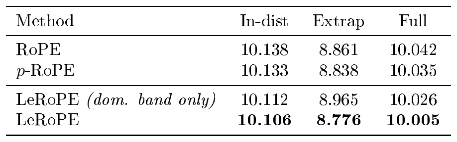
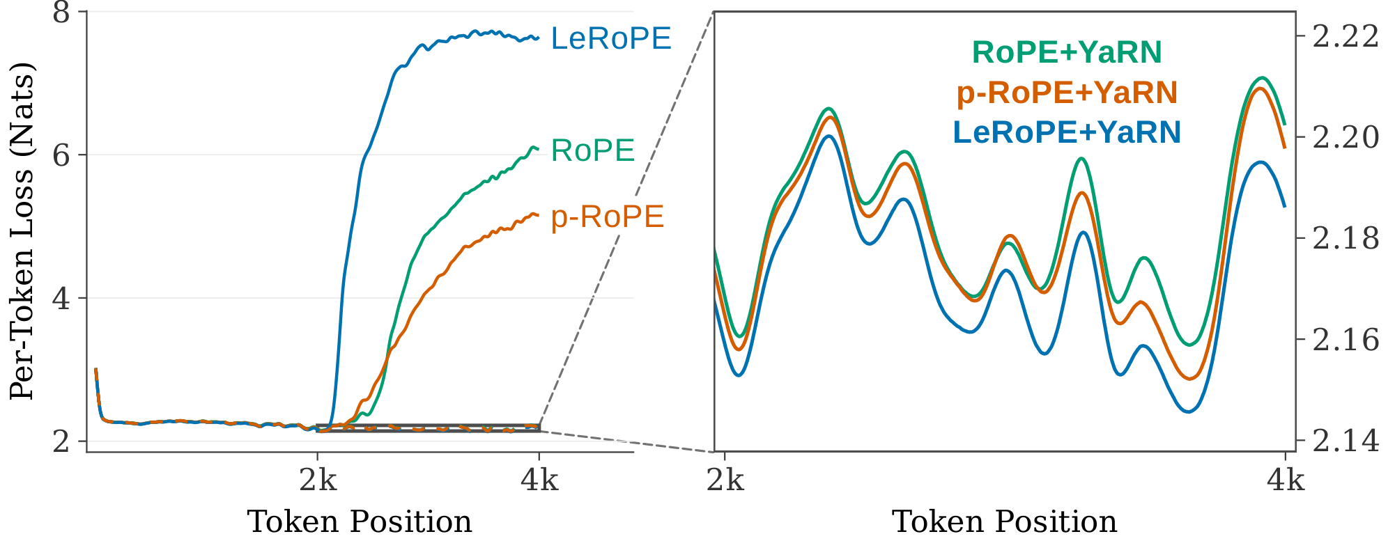
Naive Extrapolation. With unmodified positions, LeRoPE degrades more sharply than RoPE and $p$-RoPE (Appendix D.2, Figure 9). The dominant frequency band's logit contribution follows a negative half-cycle of a sinusoid with period $~\approx 2.2, L_{\text{train}}$, so within the training window it remains negative or near zero. On relative distances beyond those seen during training, the contribution becomes positive. To measure the effect of the dominant positional band alone, we measure the performance of dominant-band interpolation, which applies positional interpolation only to the dominant positional band. We find that this prevents the rapid out-of-distribution perplexity explosion, roughly matching the performance of NTK-by-parts (Table 11). For extrapolation evaluations we filter the validation set of C4 for documents longer than 4096 in length.

Compatibility with YaRN.

Standard context-extension methods transfer to LeRoPE directly. LeRoPE with NTK-by-parts scaling and YaRN's attention temperature outperforms the same recipe applied to RoPE and $p$-RoPE, and also outperforms dominant-band interpolation combined with a temperature. For each method we sweep over YaRN's temperature hyper-parameter to ensure a fair comparison. LeRoPE's in-distribution advantage therefore carries over under the extension tooling practitioners already use; the best configuration for extrapolation overall is LeRoPE with YaRN (Table 11). See Appendix D.2 for a description of NTK-by-parts and YaRN.

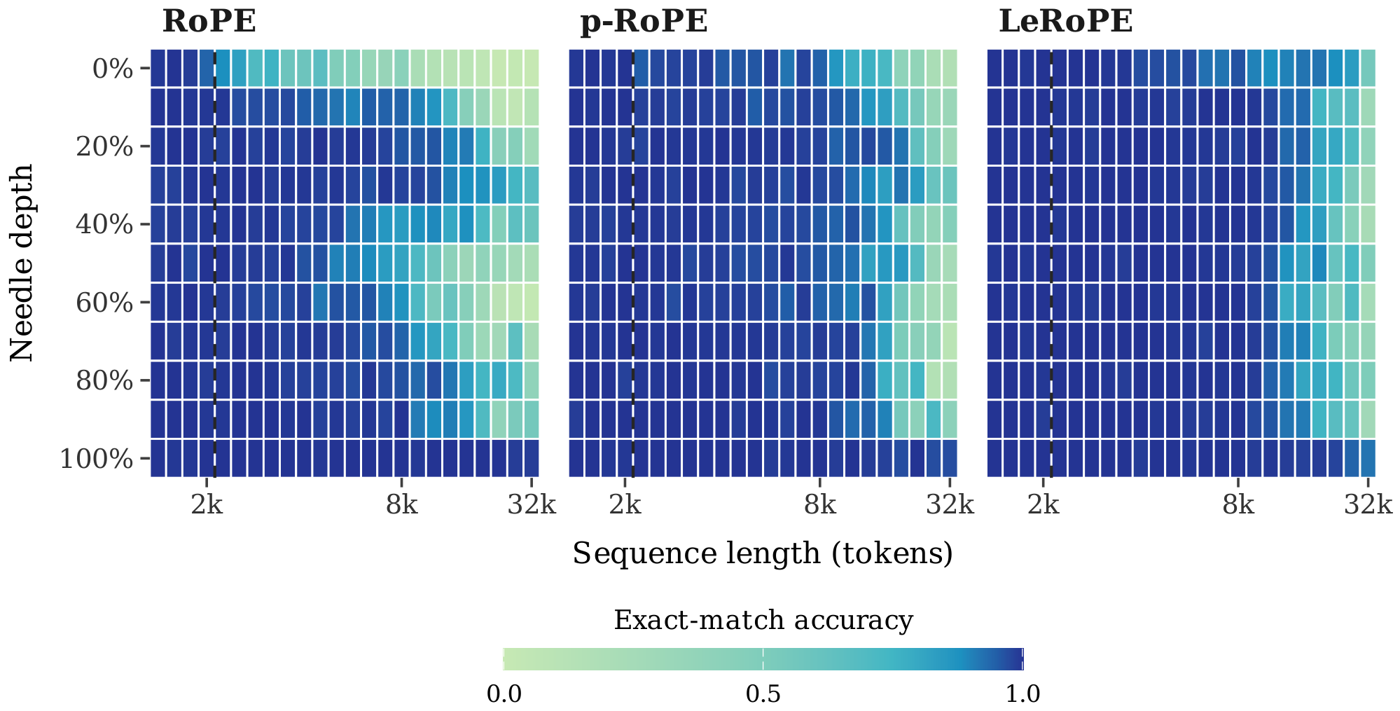
Needle-in-a-Haystack. We evaluate the 2.52B models on single-needle NIAH with YaRN at sequence lengths up to 32k. Single-needle retrieval is saturated within $L_{\text{train}}$ (§ 5.2), so accuracy beyond it isolates where retrieval breaks down with length. Averaged across needle depths, LeRoPE outperforms both RoPE and $p$-RoPE at every evaluated length (Figure 5).

8. Conclusion

Section Summary: The authors introduce LeRoPE, a variation of the standard RoPE method that allows its frequency settings to be adjusted during training using one adjustable scale for each band of frequencies. Tests across model sizes from 52 million to 2.5 billion parameters show that LeRoPE consistently beats both the original RoPE and a partial version of it, with the original approach needing about 3.4 percent more computing power to reach similar results at the biggest scale. They suggest that future studies could test whether these learned parameters also help in the local parts of models that combine local and global attention.

We propose LeRoPE, which makes RoPE's frequencies learnable through one scale per frequency band. Across a scaling ladder from 52M to 2.5B parameters, LeRoPE outperforms RoPE and partial RoPE at every scale, with RoPE requiring 3.4% more compute to match it at the largest scale. Given its consistent performance improvements on in-distribution language modeling, future work may explore the merits of learned RoPE parameters in local layers of local-global models ([6]).

9. Limitations

Section Summary: The study was limited to training models of at most 2.5 billion parameters, mostly on the C4 dataset with only minor tests involving code. These models used token counts considered optimal for scaling tests, yet they remain far less trained than the large language models in common use today. Measurements of performance differences across random training runs covered only smaller scales, while the benefits of LeRoPE for bigger, heavily trained models were not examined.

We only train models up to 2.5B parameters, and our pretraining corpus is limited to C4, with small experiments on code. Further, while Chinchilla-optimal token budgets may be sound for scaling experiments, these models are severely under-trained compared to current language models. Though cross-seed variance is measured for small model scales, runs about 608M remain trained on one seed and may contain different cross-seed variance. The gains of LeRoPE on overtrained models at larger scales remain to be shown.

Appendix

Section Summary: The appendix describes the experimental setup for testing learnable RoPE frequencies in language models, based on an Enoki scaling ladder that co-scales model depth and width while fixing head size at 64. It details numerous deviations from prior work, including use of the C4 dataset with a custom tokenizer, RMSNorm, a cosine learning-rate schedule decaying to zero, adjusted AdamW settings, larger batches, and specific initialization and weight-decay rules, along with tables listing the resulting model sizes and full hyperparameters. The text also explains two approaches to measuring compute-efficiency gains over standard RoPE baselines—one using piecewise-linear interpolation in log-compute and another fitting a parametric scaling law—while noting instability issues that can affect the estimates at larger scales.

part{}

@toptitlebar Supplementary Materials
Learnable RoPE Frequencies Improve Language Modeling @bottomtitlebar

mtcsetfeatureparttocopen

noptcrule [c]

suppressfloats[t]

A. Ladder Notes

A.1 Architecture

::: {caption="Table 3: Optimal peak learning rates per scale. All three positional-encoding methods share the same optimum at every swept scale; for the two largest models the grid index is extrapolated from the smaller scales, across which the optimum tracks eta propto 1/N_tot."}

:::

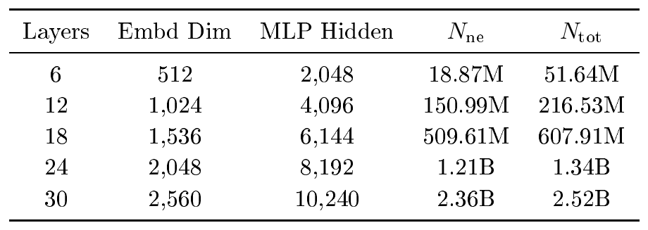
We use the Enoki scaling ladder of [25, 24]: the head dimension is fixed at 64 and depth and width are co-scaled, yielding models on the shallower, wider end. The architecture uses RoPE, pre-norm, QK-norm applied before RoPE, no biases, and no weight tying. Table 4 lists the model configurations.

We deviate from the Enoki recipe as follows:

• Data and tokenizer: C4 ([16]) with a 32, 000-token SentencePiece vocabulary, rather than FineWeb with the 50, 304-token GPT-2 tokenizer.
• Document masking: We mask attention across document boundaries within packed sequences; prior Enoki work does not state whether it does so.
• Normalization: RMSNorm in place of LayerNorm for the pre-norms, QK-norm, and final norm.
• Learning-rate schedule: cosine decay to zero rather than to $0.1\times$ peak, with a warmup of 1000 steps rather than $2%$ of total steps.
• Optimizer: AdamW with $\beta_2 = 0.95$ rather than $0.999$ ($\beta_1 = 0.9$ in both), and independent weight decay $\lambda = 8/T$, where $T$ is the total number of training steps (with weight decay of $\lambda=\omega/T$, [24] report $\omega = 4$ to be robust; both $\omega=4$ and $\omega=8$ lie within their swept range).
• Batch size: 64 sequences (global batch size of $131{,}072$ tokens) instead of 32, in line with the batch-size findings of [25] for this ladder.
• Gradient clipping: global-norm $1.0$ instead of $0.5$.

All weights are initialized with fan-in scaling, $\text{std} = 1/\sqrt{\text{fan-in}}$; the MLP and attention output projections receive an additional depth-dependent factor, $\text{std} = 1/\sqrt{2, n_{\text{layer}} \cdot \text{fan-in}}$; and token embeddings use $\text{std} = 1/\sqrt{d_{\text{embd}}}$, giving each embedding vector unit expected norm. See Table 5 for the complete set of hyper-parameters.

::: {caption="Table 4: Architectural details of our scaling ladder following [24]. Head dimension is fixed to 64 across scale, head count is tfrac43n_layer, width is d_embd = 64 × heads. We use a vocabulary of size 32,000 and include the non-embedding (N_ne) and total (N_ne) parameter counts."}

:::

::: {caption="Table 5: Training Hyperparameters"}

\begin{tabular}{l | c}
\toprule
\textbf{Parameter} & \textbf{Value} \\
\midrule
Sequence length & 2048 \\
Batch size (sequences) & 64 \\
Tokens per batch & 131, 072 \\
Vocabulary size & 32, 000 \\
Optimizer & AdamW ($\beta_1{=}0.9$, $\beta_2{=}0.95$) \\
Adam $\epsilon$ & 1e-8 \\
Warmup window & 1000 steps \\
LR rule, $\gamma(t)$ & cosine decay \\
Final LR & 0 \\
Precision/Optimizer state precision & bfloat16/float32 \\
Gradient clipping & 1.0 (global norm) \\
Weight-decay$^{1}$, $\lambda$ & $8/T$ (independent) \\
\bottomrule
\end{tabular}

• $^{1}$ $T$ denotes total training steps; weight decay omitted on LeRoPE parameters, embedding parameters, and normalization layers.

:::

A.2 Compute Multiplier Estimation

Choice of interpolation axis.

We use the piecewise-linear baseline of [24], but interpolate in $\log C$ rather than raw $C$. For compute budgets outside the ladder, we continue the nearest line segment. Loss–compute curves are convex. Linear interpolation in $C$ lies above the true curve between ladder points, so inverting this baseline overestimates the compute budget and the multiplier. With nine scales and adjacent budgets within a factor of ${\sim}2$ – $7$, the effect is small on their ladder. Across our decade-wide gaps, it is severe in $C$ but smaller in $\log C$, where the power-law curve is far straighter. At the largest scale, LeRoPE's loss is below that of every RoPE model. Estimating the multiplier requires extrapolating the RoPE curve, so the top-scale values are conservative.

Parametric alternative: efficiency gain.

The more common estimator fits a scaling law to the baseline ladder ([29, 30, 26]),

$ L = f(C) = A C^{-\alpha} + E,\tag{8} $

and reports the efficiency gain $\mathrm{EG} = f^{-1}(L')/C'$ for a variant reaching loss $L'$ at cost $C'$. Fitting the RoPE ladder gives $A = 26.4$, $\alpha = 0.0574$, and $E = 0.641$. The fitted $\alpha$ is within the range reported for fits with an irreducible term by [24], Table 15. Table 6 compares the efficiency gains with the piecewise multipliers of Section 4.2, which differ by at most $0.009$ at every scale.

\begin{tabular}{lccccc}
\toprule
  {} & 52M & 217M & 608M & 1.34B & 2.52B \\
\midrule
Piecewise $\log C$ (ours) & 1.071 & 1.048 & 1.047 & 1.032 & 1.034 \\
Efficiency gain (fitted) & 1.064 & 1.047 & 1.039 & 1.039 & 1.031 \\
\bottomrule
\end{tabular}

Fit instability in compute multiplier estimates.

With five ladder points and three parameters, the irreducible loss $E$ is weakly identified. Every $E \in [0.3, 1.0]$ fits the ladder with RMSE below $0.006$ nats (Table 7). The RMSE differences between these fits are comparable to per-run seed variability (Table 9), so run-to-run noise can move the best-fit $E$ across this range. A misspecified fit can have residuals larger than the $0.003$ – $0.010$-nat gaps being measured, whereas the piecewise estimator has no residual at measured scales. [24] report the same identifiability issue. Their fitted single-power-law exponent ranges from $0.048$ to $0.074$ as the assumed saturation level changes. Our ladder is sparser and our effect is smaller, so the problem is more severe.

\begin{tabular}{lcc ccccc}
\toprule
  {} & & & \multicolumn{5}{c}{EG per scale} \\
\cmidrule(lr){4-8}
$E$ & $\alpha$ & RMSE (nats) & 52M & 217M & 608M & 1.34B & 2.52B \\
\midrule
0.0 & 0.044 & $6.4\mathrm{e}{-3}$ & 1.028 & 1.118 & 1.090 & 1.031 & \textbf{0.952} \\
0.3 & 0.050 & $3.8\mathrm{e}{-3}$ & 1.043 & 1.089 & 1.069 & 1.034 & \textbf{0.982} \\
0.5 & 0.054 & $1.8\mathrm{e}{-3}$ & 1.055 & 1.065 & 1.052 & 1.036 & 1.008 \\
0.641 & 0.057 & $5.3\mathrm{e}{-4}$ & 1.064 & 1.047 & 1.039 & 1.039 & 1.031 \\
0.8 & 0.062 & $2.2\mathrm{e}{-3}$ & 1.075 & 1.024 & 1.022 & 1.043 & 1.063 \\
1.0 & 0.069 & $5.5\mathrm{e}{-3}$ & 1.090 & \textbf{0.989} & \textbf{0.997} & 1.051 & 1.118 \\
\bottomrule
\end{tabular}

Sharing the saturation across methods.

Following [24], we fit RoPE, $p$-RoPE, and LeRoPE jointly with a shared $E$ and per-method $(A, \alpha)$. The best fit ($E = 0.643$, joint RMSE 4.7 x 10^-4 nats) leaves the efficiency gains unchanged to within $0.001$. The identifiability window does not narrow; every shared $E \in [0.3, 1.0]$ still fits within $0.006$ nats. Because the three curves are nearly parallel, adding methods provides little information about the floor. The degeneracy comes from the range of scales, not the number of points. The fitted exponents agree to within $0.5%$ ($\alpha \in [0.0573, 0.0576]$), similarly to [24].

Richer functional forms.

[24] fit a double power law $L = a + bC^{-c} + eC^{-f}$ across five optimizer curves with a shared saturation $a$. It is identifiable with ${\sim}10$ scales per curve, but our five-point ladder has no residual degrees of freedom. A hinge-type broken power law ([31]) fits our ladder worse than the saturating form (RMSE 1.1 x 10^-3 vs. 5.3 x 10^-4 nats), recovers nearly equal exponents on both sides of a weakly identified break, and exhibits the same efficiency-gain instability, including values below $1$. The ladder favors saturation over a break.

We therefore report efficiency gain as corroboration and keep the piecewise estimator primary.

A.3 Seed Variability

Seeds control model initialization and data ordering. To bound their effect, we repeat the 217M runs (as well as RoPE with two additional bases) and the 608M runs under three matched seeds (Table 9). All comparisons are within a seed: the two runs share initialization draws and data order, so their loss fluctuations are strongly correlated and the paired margins vary far less than the marginal deviations ($s_d = 0.0019$ vs. $\sigma$ up to $0.0020$ at 217M; 5 $s_d = 0.0010$ at 608M). LeRoPE improves on every baseline under every 5 individual seeds at both scales, and per-method variability decreases with scale ($\sigma_{\text{LeRoPE}}$: $0.0019 \to 0.0004$), supporting the reading that the unseeded larger-scale gaps in Table 1 also exceed noise.

B. Gradient Dynamics

For clarity in this section, we will omit the pre-softmax scaling factor $1/\sqrt{d}$, operate on a single head, and take $o_i$ to be the post-softmax accumulation of values before output projection $W_o$.

B.1 Definitions and Lemmas

We begin with the following definitions:

$ \begin{aligned} g_s &\triangleq \frac{\partial \mathcal{L}}{\partial o_s} \ S_{st}^{(m)} &\triangleq (s-t)|q_s^{(m)}||k_t^{(m)}| \sin \left(\phi_{st}^{(m)} + (s-t)\theta^{(m)} \right) \ C_m(\delta) &\triangleq \sum_{\substack{s, t \s-t=\delta}} \alpha_{st} |q_s^{(m)} | |k_t^{(m)}| e^{i\phi_{st}^{(m)}} (v_t - o_s)^T g_s \ P(\theta) &= \text{Re}\left(\sum_{\delta=1}^{L-1} C(\delta) e^{i \delta \theta} \right) \end{aligned}\tag{9} $

########## {caption="Lemma 2"}

Let $g_s = \partial \mathcal{L} / \partial o_s$ be the gradient of the loss with respect to output vector $o_s$. Let $\partial \mathcal{L} / \partial D_{st}^{(m)}$ be the gradient of the loss with respect to the dot product produced by band $m$ from query position $s$ to key position $t$.

Then $\partial \mathcal{L} / \partial D_{st}^{(m)} = \alpha_{st} g_s^T(v_t - o_s)$.

Proof: First, note that the only effect of the value $D_{st}^{(m)}$ is through its effect on the output vector at position $s$, $o_s$.

Thus, we have:

$ \begin{aligned} \frac{\partial \mathcal{L}}{\partial D_{st}^{m}} &= \left(\frac{\partial \mathcal{L}}{\partial o_s} \right)^T \left(\frac{\partial o_s}{\partial D^{(m)}{st}} \right) \ &= g_s^T \left(\frac{\partial o_s}{\partial D^{(m)}{st}} \right) \end{aligned} $

So we only have to find the partial derivative of $o_i$ with respect to the band- $s$ $QK$ product.

The softmax Jacobian gives:

$ \begin{aligned} \frac{\partial o_s}{\partial z_{st}} &= \sum_{t' < s} \alpha_{st'}(\mathbb{1}[t=t'] - \alpha_{st})v_{t'} \ &= \alpha_{st}(v_t - o_s) \ \frac{\partial z_{st}}{\partial D_{st}^{(m)}} &= 1 \ \implies \frac{\partial o_s}{\partial D_{st}^{(m)}} &= \alpha_{st}(v_t - o_s) \ \implies \frac{\partial \mathcal{L}}{\partial D_{st}^{(m)}} &= \alpha_{st} g_s^T (v_t - o_s) \end{aligned} $

########## {caption="Lemma 3"}

Define $P_m(\theta)$ as the real component of the discrete-time Fourier Transform of the signal $C_m(\delta)$ with frequency $\theta$, as above.

Then $\frac{\partial \mathcal{L}}{\partial \theta^{(m)}} = P_m'(\theta^{(m)})$.

Proof:

First, consider the full sum from Equation 6. We may split the sum by relative offsets $\delta \triangleq s - t$, and for notational compactness define $g_{st}^{(m)} \triangleq \partial \mathcal{L} / \partial D_{st}^{(m)}$

$ \begin{aligned} \frac{\partial \mathcal{L}}{\partial \theta^{(m)}} &= - \sum_{t < s} \left(s - t\right)| q_s | |k_t | \sin \left(\phi_{st} + (s - t)\theta^{(m)} \right) \frac{\partial \mathcal{L}}{\partial D_{st}^{(m)}} \ &= -\sum_{\delta = 1}^{L-1} \sum_{\substack{s, t \ s-t = \delta}} \delta , | q_s | | k_{t} | \sin \left(\phi_{st} + \delta \theta^{(m)} \right) g_{st}^{(m)} \ &= -\sum_{\delta = 1}^{L-1} \sum_{\substack{s, t \ s-t = \delta}} \delta , | q_s | | k_{t} | \sin \left(\phi_{st} + \delta \theta^{(m)} \right) \alpha_{st} (v_t - o_s)^T g_s \end{aligned} $

To split the sine, write it as an exponential and note that all scalar terms outside of the sine are real, allowing us to apply the imaginary operator across the final summed value:

$ \begin{aligned} \frac{\partial \mathcal{L}}{\partial \theta^{(m)}} &= -\sum_{\delta = 1}^{L} \sum_{\substack{s, t \ s-t=\delta}} \delta \text{Im}\left(e^{i\phi_{st}} e^{i \delta \theta^{(m)}}\right) |q_s | |k_t| \alpha_{st} (v_t - o_s)^T g_s \ &= -\text{Im}\left(\sum_{\delta = 1}^{L-1} \sum_{\substack{s, t \s-t=\delta}} \delta e^{i\phi_{st}} e^{i \delta \theta^{(m)}} |q_s | |k_t| \alpha_{st}(v_t - o_s)^T g_s \right) \ &= -\text{Im}\left(\sum_{\delta = 1}^{L-1} \delta e^{i \delta \theta^{(m)}} \sum_{\substack{s, t \s-t=\delta}} e^{i\phi_{st}} |q_s | |k_t| \alpha_{st} (v_t - o_s)^T g_s\right) \ &= -\text{Im}\left(\sum_{\delta = 1}^{L-1} \delta C(\delta) e^{i \delta \theta^{(m)}} \right) \ &= -\text{Im}\left(\sum_{\delta = 1}^{L-1} \left(-i \frac{d}{d \theta^{(m)}} \left[C(\delta) e^{i \delta \theta^{(m)}}\right]\right) \right) \ &= \frac{d}{d \theta^{(m)}} \text{Re}\left(\sum_{\delta = 1}^{L - 1} C(\delta) e^{i \delta \theta^{(m)}} \right) \ &= P'_m(\theta^{(m)}) \end{aligned} $

########## {caption="Lemma 4"}

As previously, define $S_{st}^{(m)}$ to be the offset-weighted sine term at RoPE-band $m$; let $v_t$ be the attention value vector at position $s$ and $g_s$ be the downstream loss gradient $\partial \mathcal{L} / \partial o_s$. Then the gradient with respect to RoPE parameter $\theta^{(m)}$ is as follows:

$ \frac{\partial \mathcal{L}}{{\partial \theta^{(m)}}} = - \sum_{s} \text{Cov}{t ~\sim p_s(t)} \left(v_t^T g_s, S{st}^{(m)} \right) $

Proof: As in Lemma 3, note

$ \begin{aligned} \frac{\partial \mathcal{L}}{\partial \theta^{(m)}} &= -\sum_{s=1}^{s_{max}} \sum_{t = 0}^{s-1} \alpha_{st} (s-t) , | q_s | | k_{t} | \sin \left(\phi_{st} + (s-t) \theta^{(m)} \right) (v_t - o_s)^T g_s \ &= -\sum_{s=1}^{s_{max}} \sum_{t = 0}^{s-1} \alpha_{st} S_{st}^{(m)} (v_t - o_s)^T g_s \ &= -\sum_{s=1}^{s_{max}} \mathbb{E}{t ~\sim p_s(t) } \left[S{st}^{(m)} (v_t - o_s)^T g_s \right] \end{aligned} $

Now, note that $\mathbb{E}{t ~\sim p_s(t)} [(v_t - o_s)^Tg_s] = 0$, as $\mathbb{E}{t ~\sim p_s(t)} [v_t] = o_s$, and $g_s$ factors out.

Thus, the expected product of the two terms equals their covariance.

So, as desired, we obtain:

$ \begin{aligned} \frac{\partial \mathcal{L}}{\partial \theta^{(m)}} &= -\sum_{s=1}^{s_{max}} \text{Cov} \left(S_{st}^{(m)}, v_t^T g_s \right) \end{aligned} $

In expectation, with enough samples, in the absence of periodic structure in downstream attention-logit gradients, we would expect this update term to remain centered roughly around zero.

B.2 Phasor Plots

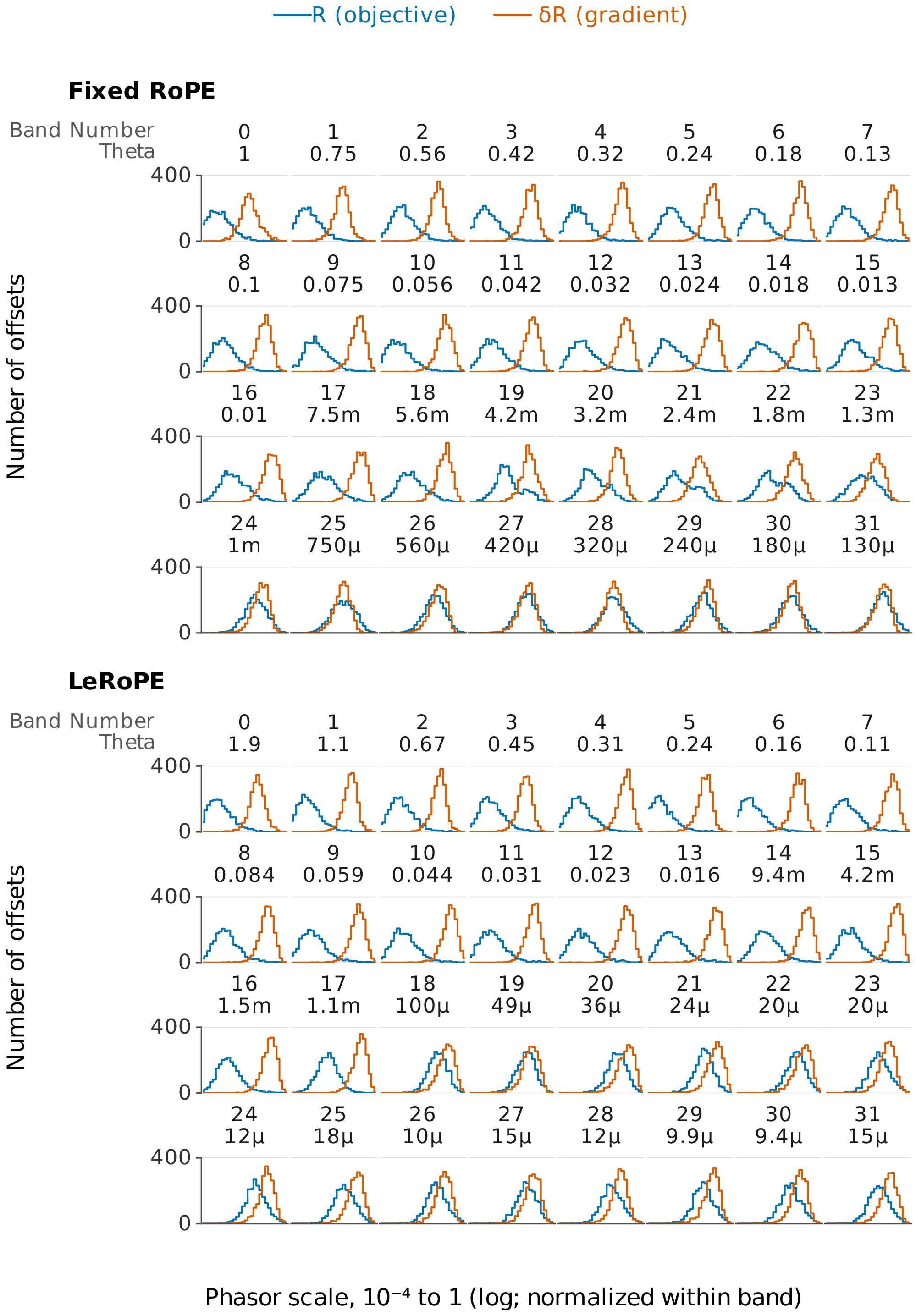
In Figure 7, we plot the per-offset gradient phasors for all bands, for both LeRoPE and RoPE models. The final gradient corresponds to the real component of the aggregate phasor. The dashed line denotes the direction of this aggregate phasor, and the red dot the aggregate phasor, normalized between 0 (full cancellation) and 1 (full coherence).

Gradient (length-weighted) phasors take on similar scales across offsets, as compared to the non-length-weighted objective phasors. This phenomenon is visible in Figure 6.

C. Additional Ablations

\begin{tabular}{lcc}
\toprule
Variant & Val loss (nats) & $\Delta$ vs RoPE \\
\midrule
RoPE, $b = 2048$ $^\dagger$ & 2.9107 & $+0.0073$ \\
RoPE, $b = 10{,}000$ (default)$^\dagger$ & 2.9035 & --- \\
RoPE, $b = 500{,}000$ $^\dagger$ & 2.8996 & $-0.0039$ \\
\midrule
$p$-RoPE, $p = 0.25$ & 2.9208 & $+0.0173$ \\
$p$-RoPE, $p = 0.5$ & 2.9029 & $-0.0006$ \\ 
$p$-RoPE, $p = 0.75$ (baseline) & 2.9029 & $-0.0006$ \\
\midrule
LeRoPE (log scalar, shared)$^\dagger$ & \textbf{2.8978} & $\mathbf{-0.0057}$ \\
\quad linear scalar & 2.8978 & $-0.0057$ \\
\quad direct frequencies & 2.8980 & $-0.0055$ \\
\quad per layer and head & 2.8996 & $-0.0039$ \\
\quad frozen transferred freqs. (Fixed LeRoPE) & 2.8999 & $-0.0036$ \\
\bottomrule
\end{tabular}

In this section we include additional ablations that we ran during the process of testing LeRoPE.

Parametrization. LeRoPE learns the per-band scale in log space, $\hat\theta_m = e^{\alpha_m}\theta_m$. We compare against a linear scalar, $\hat\theta_m = \alpha_m \theta_m$, and against directly learning each frequency, $\hat\theta_m = \alpha_m$. Both recover RoPE at initialization.

All three reach the same loss to within $0.0003$ nats (Table 8), within seed variability, suggesting the choice is not critical with Adam's per-parameter step normalization. However, we observed very unstable trajectories for the directly learned frequencies and aliasing around 0 for the linear scalars. We retain the log parametrization because it removes these issues.

Finer Learned Granularities. LeRoPE shares one set of scales across all layers and heads. Learning a separate set per layer and head adds parameters but no benefit. It reached $2.8996$ nats, $0.0018$ behind shared LeRoPE which is within one seed standard deviation (Table 8).

Change of RoPE Base. Prior work finds $b = 10{,}000$ can be suboptimal, with gains reported from both raising and lowering the base ([23]). We train RoPE with $b = L_{\text{train}} = 2048$, following FMRoPE ([9]), and $b = 500{,}000$, the value adopted for long-context models ([32]) (Table 9). Matching the base to the training length degrades in-window loss on every seed ($+0.0069$ nats), consistent with the in-window side of the interpolation–extrapolation trade-off; raising it to $500{,}000$ improves loss on every seed ($-0.0038$ nats), capturing roughly $60%$ of LeRoPE's gain. LeRoPE outperforms every tested base under every seed (Table 9).

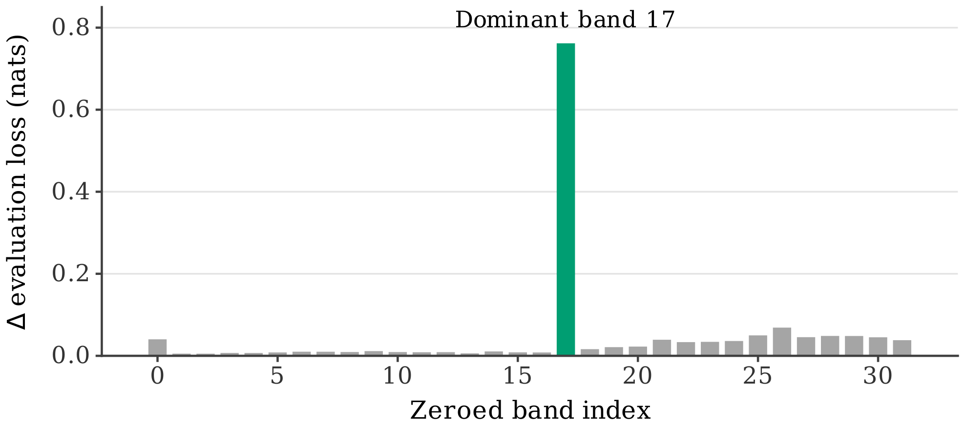
$p$-RoPE fraction. Our baseline uses $p = 0.75$, the best-performing value in [7]. We swept $p \in { 0.25, 0.5, 0.75}$ at 217M. $p = 0.5$ matches $p = 0.75$ (both within seed variability of RoPE). $p = 0.25$ leaves no band rotating with a period beyond ${\sim}50$ tokens and degrades substantially ($+0.0173$ nats, ${\sim}9\times$ seed variability). Notably, LeRoPE's learned suppression point at $L_{\text{train}} = 2048$ sits near the same boundary (band ${\sim}17$ of 32, an effective $p \approx 0.5$), while its gain comes from reshaping the bands it retains, which no choice of $p$ can express.

\begin{tabular}{lccccc}
\toprule
  {} & Seed 42 & Seed 43 & Seed 44 & mean $\pm$ std & $\bar\Delta$ \\
\midrule
\multicolumn{6}{l}{\emph{217M}} \\
RoPE ($b{=}2048$) & 2.9107 & 2.9100 & 2.9137 & $2.9115{\pm}0.0020$ & 0.0134 \\
RoPE ($b{=}10$ k) & 2.9035 & 2.9050 & 2.9053 & $2.9046{\pm}0.0010$ & 0.0066 \\
RoPE ($b{=}500$ k) & 2.8996 & 2.8997 & 2.9031 & $2.9008{\pm}0.0020$ & 0.0027 \\
LeRoPE & \textbf{2.8978} & \textbf{2.8963} & \textbf{2.9001}
   {} & $\mathbf{2.8981{\pm}0.0019}$ & --- \\
\midrule
\multicolumn{6}{l}{\emph{608M}} \\
RoPE ($b{=}10$ k) & 2.6304 & 2.6290 & 2.6288 & $2.6294{\pm}0.0009$ & 0.0040 \\
LeRoPE & \textbf{2.6253} & \textbf{2.6250} & \textbf{2.6257}
   {} & $\mathbf{2.6254{\pm}0.0004}$ & --- \\
\bottomrule
\end{tabular}

D. Extrapolation and Dominant Band Wavelengths

D.1 Dominant Positional Band Wavelength

\begin{tabular}{lcccccc}
\toprule
Scale (params) & $L$ & Dominant Band & $e^\alpha$ & $\hat{\theta}^{(m)}$ & $\lambda_{dominant}$ (tok) & $\hat{\theta}^{(m)} L$ \\
\midrule
217M & 2048 & 16 & 0.1481 & 0.001481 & 4243.3 & 3.033 \\
217M & 4096 & 18 & 0.1178 & 0.000663 & 9481.7 & 2.714 \\
217M & 8192 & 19 & 0.0823 & 0.000347 & 18097.8 & 2.844 \\
608M & 2048 & 17 & 0.1945 & 0.001459 & 4307.8 & 2.987 \\
1.34B & 2048 & 17 & 0.1955 & 0.001466 & 4285.6 & 3.003 \\
2.52B & 2048 & 17 & 0.2009 & 0.001507 & 4170.3 & 3.086 \\
\bottomrule
\end{tabular}

Leave-one-out band ablation.

We zero one learned frequency band at a time and measure the increase in evaluation loss relative to the baseline. Zeroing band 17 increases loss by $0.762$ nats. The next-largest loss increase comes from zeroing band 26, which increases loss by only $0.069$ nats.

D.2 Extrapolation Details

NTK-by-parts.

NTK-by-parts ([28]) sets each band's interpolation from its number of rotations during training. For band $m$ with frequency $\varphi_m$, let $r_m = L_{\text{train}}\varphi_m / 2\pi$ be its rotation count during training. In LeRoPE, $\varphi_m=\hat\theta_m$. Let $s = \min(1, L_{\text{train}}/L_{\text{doc}})$ be the per-document position interpolation factor. We multiply each frequency by $M_m = s + w_m(1-s)$, where $w_m = \mathrm{clip}\big((r_m-r_{lo})/ (r_{hi}-r_{lo}), , 0, , 1\big)$, with $r_{lo}=1$ and $r_{\text{hi}}=32$ ([28]). Bands with fewer than $r_{\text{lo}}$ rotations are scaled by $s$, while bands with more than $r_{\text{hi}}$ rotations are unchanged. Between these thresholds, the multiplier increases linearly. We apply interpolation per document rather than at a fixed target length and compute rotation counts from each model's own frequencies. LeRoPE's dominant band, slowed to ${\sim}0.5$ rotations per window, is always fully interpolated.

YaRN.

YaRN ([28]) adds an attention temperature to NTK-by-parts to keep attention from flattening at longer contexts. With per-document extension factor $s_{\text{ext}} = \max(1, L_{\text{doc}}/L_{\text{train}})$, attention logits are multiplied by $(c \ln s_{\text{ext}} + 1)^2$ before the softmax. We sweep YaRN's temperature coefficient $c$ for each method and use $c=0.1$, matching [28]. Both mechanisms operate at inference only; no parameters are updated.

::: {caption="Table 11: Average perplexity for 2.52B models under NTK-by-parts + YaRN as well as LeRoPE with only interpolating the dominant band and extrapolating the rest. Split by in-distribution (<L_train) and extrapolated (>= L_train) positions over the 0–4095 window. LeRoPE is lowest in every column."}

:::

To complement these sequence-level averages, Figure 9 shows per-token loss over the full evaluation range and a zoomed view of the extrapolation region.

E. Code Pretraining

We evaluate LeRoPE on the Python split of the StarCoder data ([33]) to test whether its gains and frequency patterns in Section 6 are specific to C4 or generalize to code. We pre-train 217M-parameter models with the same setup as Section 4, using a 32,000-token SentencePiece tokenizer trained on code to match vocabulary size and parameter count.

Language modeling.

At 217M, LeRoPE improves over RoPE by $0.0104$ nats (Table 12). By contrast, $p$-RoPE improves by $0.0006$ nats, The StarCoder-Python runs use a single seed. If we assume run-to-run variability is comparable to C4 (Table 9), LeRoPE's $0.0104$-nat loss reduction exceeds that variability several times over.

\begin{tabular}{lcc}
\toprule
Method & Val loss (nats) & $\Delta$ vs RoPE \\
\midrule
RoPE & 1.2501 & --- \\
$p$-RoPE & 1.2495 & -0.0006 \\
LeRoPE & \textbf{1.2398} & -0.0104 \\
\bottomrule
\end{tabular}

Learned frequencies.

We analyze 217M-parameter code models trained at $L_{\text{train}} \in {2048, 4096, 8192}$ following the procedure in Section 6. On StarCoder, fast bands remain close to their fixed-RoPE frequencies while slow bands learn wavelengths substantially longer than their fixed-RoPE values, as on C4 (Figure 3 c). As training length increases, learned frequencies deviate from fixed RoPE at lower frequencies. The dominant wavelength also increases, from $5{,}250$ tokens at $L_{\text{train}}=2048$ to $16{,}627$ tokens at $L_{\text{train}}=8192$. At $L_{\text{train}}=2048$, a single positional band dominates (Figure 10 b) with wavelength $\lambda \approx 5{,}250$ tokens.

References

Section Summary: The references section provides a bibliography of academic papers, technical reports, and conference proceedings cited in the main text. These sources primarily cover foundational work on transformer models and attention mechanisms, along with later research on rotary positional encodings, large language models such as LLaMA and PaLM, and techniques for improving context length handling. The entries span from 2017 to 2026 and include both arXiv preprints and peer-reviewed publications.

[1] Ashish Vaswani et al. (2017). Attention is All you Need. In Neural Information Processing Systems. https://api.semanticscholar.org/CorpusID:13756489.

[2] Jianlin Su et al. (2021). RoFormer: Enhanced Transformer with Rotary Position Embedding. ArXiv. abs/2104.09864. https://api.semanticscholar.org/CorpusID:233307138.

[3] Hugo Touvron et al. (2023). LLaMA: Open and Efficient Foundation Language Models. ArXiv. abs/2302.13971. https://api.semanticscholar.org/CorpusID:257219404.

[4] Aakanksha Chowdhery et al. (2022). PaLM: Scaling Language Modeling with Pathways. ArXiv. abs/2204.02311. https://api.semanticscholar.org/CorpusID:247951931.

[5] Albert Qiaochu Jiang et al. (2023). Mistral 7B. ArXiv. abs/2310.06825. https://api.semanticscholar.org/CorpusID:263830494.

[6] Gemma Team Aishwarya Kamath et al. (2025). Gemma 3 Technical Report. ArXiv. abs/2503.19786. https://api.semanticscholar.org/CorpusID:277313563.

[7] Federico Barbero et al. (2024). Round and Round We Go! What makes Rotary Positional Encodings useful?. ArXiv. abs/2410.06205. https://api.semanticscholar.org/CorpusID:273229201.

[8] Xin Men et al. (2024). Base of RoPE Bounds Context Length. ArXiv. abs/2405.14591. https://api.semanticscholar.org/CorpusID:269983770.

[9] Yui Oka et al. (2026). Frequency Bands in RoPE: Base Frequency and Context Length Shape the Interpolation–Extrapolation Trade-off. In The Fourteenth International Conference on Learning Representations. https://openreview.net/forum?id=PR1PPxvG9Q.

[10] Alec Radford et al. (2019). Language Models are Unsupervised Multitask Learners. https://api.semanticscholar.org/CorpusID:160025533.

[11] Jacob Devlin et al. (2019). BERT: Pre-training of Deep Bidirectional Transformers for Language Understanding. In North American Chapter of the Association for Computational Linguistics. https://api.semanticscholar.org/CorpusID:52967399.

[12] Yinhan Liu et al. (2019). RoBERTa: A Robustly Optimized BERT Pretraining Approach. ArXiv. abs/1907.11692. https://api.semanticscholar.org/CorpusID:198953378.

[13] Susan Zhang et al. (2022). OPT: Open Pre-trained Transformer Language Models. ArXiv. abs/2205.01068. https://api.semanticscholar.org/CorpusID:248496292.

[14] Alexey Dosovitskiy et al. (2020). An Image is Worth 16x16 Words: Transformers for Image Recognition at Scale. ArXiv. abs/2010.11929. https://api.semanticscholar.org/CorpusID:225039882.

[15] Shaw et al. (2018). Self-Attention with Relative Position Representations. In Proceedings of the 2018 Conference of the North American Chapter of the Association for Computational Linguistics: Human Language Technologies, Volume 2 (Short Papers). pp. 464–468. doi:10.18653/v1/N18-2074. https://aclanthology.org/N18-2074/.

[16] Colin Raffel et al. (2019). Exploring the Limits of Transfer Learning with a Unified Text-to-Text Transformer. J. Mach. Learn. Res.. 21. pp. 140:1-140:67. https://api.semanticscholar.org/CorpusID:204838007.

[17] Ofir Press et al. (2021). Train Short, Test Long: Attention with Linear Biases Enables Input Length Extrapolation. ArXiv. abs/2108.12409. https://api.semanticscholar.org/CorpusID:237347130.

[18] Olga Golovneva et al. (2024). Contextual Position Encoding: Learning to Count What's Important. ArXiv. abs/2405.18719. https://api.semanticscholar.org/CorpusID:270094992.

[19] Songlin Yang et al. (2025). PaTH Attention: Position Encoding via Accumulating Householder Transformations. ArXiv. abs/2505.16381. https://api.semanticscholar.org/CorpusID:278789395.

[20] Sophie Ostmeier et al. (2024). LieRE: Lie Rotational Positional Encodings. In International Conference on Machine Learning. https://api.semanticscholar.org/CorpusID:276422590.

[21] Yui Oka et al. (2026). Probing Rotary Position Embeddings through Frequency Entropy. In The Fourteenth International Conference on Learning Representations. https://openreview.net/forum?id=1JZuEDq62N.

[22] Amirhossein Kazemnejad et al. (2023). The Impact of Positional Encoding on Length Generalization in Transformers. ArXiv. abs/2305.19466. https://api.semanticscholar.org/CorpusID:258987259.

[23] Xiaoran Liu et al. (2023). Scaling Laws of RoPE-based Extrapolation. ArXiv. abs/2310.05209. https://api.semanticscholar.org/CorpusID:263828829.

[24] Damien Ferbach et al. (2026). Logarithmic-time Schedules for Scaling Language Models with Momentum. https://api.semanticscholar.org/CorpusID:285303683.

[25] Zachary Charles et al. (2025). Communication-Efficient Language Model Training Scales Reliably and Robustly: Scaling Laws for DiLoCo. ArXiv. abs/2503.09799. https://api.semanticscholar.org/CorpusID:276961579.

[26] The Microsoft AI Team (2026). MAI-Thinking-1: Building a Hill-Climbing Machine. https://microsoft.ai/pdf/mai-thinking-1.pdf.

[27] Shouyuan Chen et al. (2023). Extending Context Window of Large Language Models via Positional Interpolation. ArXiv. abs/2306.15595. https://api.semanticscholar.org/CorpusID:259262376.

[28] Bowen Peng et al. (2023). YaRN: Efficient Context Window Extension of Large Language Models. ArXiv. abs/2309.00071. https://api.semanticscholar.org/CorpusID:261493986.

[29] Jared Kaplan et al. (2020). Scaling Laws for Neural Language Models. https://arxiv.org/abs/2001.08361. arXiv:2001.08361.

[30] Jordan Hoffmann et al. (2022). Training Compute-Optimal Large Language Models. https://arxiv.org/abs/2203.15556. arXiv:2203.15556.

[31] Ethan Caballero et al. (2023). Broken Neural Scaling Laws. https://arxiv.org/abs/2210.14891. arXiv:2210.14891.

[32] Wenhan Xiong et al. (2023). Effective Long-Context Scaling of Foundation Models. https://arxiv.org/abs/2309.16039. arXiv:2309.16039.

[33] Raymond Li et al. (2023). StarCoder: may the source be with you!. arXiv:2305.06161.