Probabilistic Tiny Recursive Model

Amin Sghaier
Mila – Quebec AI Institute
ILLS & ETS Montreal

Ali Parviz
Mila – Quebec AI Institute

Alexia Jolicoeur-Martineau
Independent

{amin.sghaier, ali.parviz}@mila.quebec
[email protected]

Abstract

Tiny Recursive Models (TRM) solve complex reasoning tasks with a fraction of the parameters of modern large language models (LLMs) by iteratively refining a latent state and final answer. While powerful, their deterministic recursion can lead to convergence at suboptimal solutions, without escape mechanism. A common workaround relies on task-specific input perturbations at test time combined with answer aggregation via voting. We introduce Probabilistic TRM (PTRM), a task-agnostic framework for test-time compute scaling that addresses this limitation through stochastic exploration. PTRM injects Gaussian noise at each deep recursion step, enabling parallel trajectories to explore diverse solution basins, and selects among them using the model’s existing Q head (used for early stopping in the original TRM). Without requiring retraining or task-specific augmentations, PTRM enables substantial accuracy gains across benchmarks, including Sudoku-Extreme (87.4% to 98.75%) and on various puzzles from Pencil Puzzle Bench (62.6% to 91.2%). On the latter, PTRM achieves nearly double the accuracy of frontier LLMs (91.2% vs. 55.1%) at less than 0.0001x the cost, using only 7M parameters.

Executive Summary: Probabilistic Tiny Recursive Models (PTRM) address a practical limitation in Tiny Recursive Models (TRM), a class of compact recursive networks that solve complex constraint-satisfaction puzzles with only a few million parameters. Although TRMs refine a latent state iteratively to reach correct answers, their deterministic recursion often traps trajectories in suboptimal latent basins from which they cannot escape, capping accuracy well below the model’s potential.

The work sets out to create a simple, task-agnostic way to scale test-time compute for any pretrained TRM without retraining or puzzle-specific augmentations. The method runs K parallel rollouts per puzzle, injecting scaled Gaussian noise into the latent state at every recursion step. This produces diverse trajectories; the model’s existing Q head, already trained as a correctness predictor, then selects the single best final answer.

Experiments evaluated PTRM on held-out subsets of Pencil Puzzle Bench (five puzzle types), Sudoku-Extreme, Maze-Hard, and ARC-AGI-2, using the same TRM checkpoints (5–7 M parameters) and comparing against deterministic TRM, direct-prediction baselines, and frontier large language models. Key metrics were accuracy at varying rollout counts K and supervision depths, plus estimated dollar cost per puzzle.

The largest gains appear on the hardest tasks for deterministic TRM: aggregate accuracy on Pencil Puzzle Bench rose from 62.6 % to 91.2 % at K = 100, while Sudoku-Extreme accuracy climbed from 87.4 % to 98.75 %. On the same Pencil Puzzle Bench golden set, PTRM exceeded the strongest single LLM (34.7 %) and even an ensemble of seven frontier models (55.1 %) while costing less than 0.0001× as much. Width scaling via stochastic rollouts delivered substantially larger improvements than simply increasing recursion depth, and the Q head proved a reliable verifier on most benchmarks, with best-Q@K staying within 1–2 points of the oracle pass@K ceiling.

These results show that a 7 M-parameter recursive model can now match or surpass today’s largest language models on structured reasoning at negligible cost, provided a modest amount of parallel inference compute is available. The approach therefore offers a practical route to high-accuracy puzzle solving without relying on ever-larger models or task-specific engineering.

Practitioners should adopt PTRM with K ≈ 100 and moderate noise scales (0.2–1.0) for immediate accuracy gains on similar puzzle domains. Where the gap between pass@K and best-Q@K remains noticeable (for example on Maze-Hard), a stronger learned verifier would close most of the remaining headroom. Further validation on larger grids, additional puzzle types, and non-puzzle reasoning tasks is required before broader deployment claims can be made; current results are limited to 9×9–10×10 grids and a modest number of puzzle families.

1. Introduction

Section Summary: Tiny Recursive Models achieve strong results on complex reasoning tasks by recursively refining an internal state to produce a single deterministic answer, but this approach often traps them in unproductive regions of that state space and leaves many solvable problems unanswered. The proposed Probabilistic TRM method addresses the limitation by running several parallel rollouts of the same puzzle, each perturbed by injected noise, so that different candidate answers emerge from distinct trajectories. A jointly trained quality-estimation head then selects the most promising answer among them, yielding large accuracy gains at test time with no changes to training or architecture.

Tiny Recursive Models (TRM) ([1]) achieve strong performance on complex reasoning puzzles with orders of magnitude fewer parameters than the large language models (LLMs) they outperform on tasks like Sudoku-Extreme ([2]) and ARC-AGI ([3, 4]). TRM and its predecessor Hierarchical Reasoning Model (HRM) ([2]) represent an emerging architectural alternative to standard autoregressive reasoning models. Rather than autoregressively generating chains of token-level reasoning, they recursively refine a latent state. This approach produces a single deterministic answer per input, fitting well with tasks where the answer is unique.

Despite their strong performance, their deterministic inference does not make full use of their capabilities. We show that many of TRM's incorrect answers are from rollouts trapped in bad latent space basins (i.e., regions of the latent space which decode to incorrect answers and from which the deterministic recursions cannot escape). This observation, which aligns with recent mechanistic work on related models ([5]), suggests that TRM has the capabilities to solve significantly more problems but is limited by its standard inference procedure.

Although each puzzle has a unique correct answer, many distinct latent trajectories can reach it. This is analogous to reasoning LLMs, where many reasoning trajectories can lead to the same unique answer. However, being non-deterministic, LLMs can be randomly sampled in order to form different trajectories (including Chains of Thought and actual answer). By then selecting a trajectory using a voting mechanism or based on the answer's projected value (via a verifier), LLMs can leverage test-time compute to achieve very high accuracy ([6]). We propose a way to achieve similar test-time scaling performance gains by sampling stochastic latent trajectories, each producing a deterministic decoded answer, and selecting among the answers using the model's own Q head.

TRM's Q head is trained jointly (as a correctness classifier) with the rest of the network and is conventionally used only at training time for adaptive computation (ACT) ([7]). It carries valuable information that the standard inference procedure discards.

We propose Probabilistic TRM (PTRM), a test-time compute scaling framework that introduces a new width scaling axis. At inference we run $K$ parallel rollouts per puzzle, each receiving Gaussian noise injected into the latent at every deep recursion step. The noise causes rollouts to follow different latent trajectories and settle in different basins. Among the resulting candidate answers, the Q head is used to select the one most likely to be correct. PTRM requires no training changes and no task-specific test-time augmentation, yet, as illustrated in Figure 1, delivers substantial accuracy gains across diverse reasoning benchmarks.

2. Background: Tiny Recursive Model

Section Summary: The Tiny Recursive Model is a compact neural network that repeatedly refines its own answer to a question by maintaining and updating an internal reasoning state. It performs a series of updates in which the internal state is revised several times before the answer is adjusted, and this cycle is stacked across multiple steps; training uses repeated supervision on the same examples while detaching prior states, along with an early-stopping signal that halts work on problems already solved correctly. At test time the process can simply continue for extra steps to improve accuracy, though the model can still become trapped in incorrect solutions.

Tiny Recursive Model (TRM) is a single network that iteratively refines a predicted answer $y$ to a question $x$ through recursive updates of a reasoning latent $z$. Specifically, a single latent recursion consists of $n$ updates to the latent state $z$ followed by one update to the predicted answer $y$, all using the same two-layer network $f_{\theta}$: $z \leftarrow f_\theta(x + y + z)$ $n$ times, then $y \leftarrow f_\theta(y + z)$.

$f_{\theta}$ distinguishes the two update types by whether the input includes $x$. A deep recursion runs $T$ latent recursions in sequence, with only the final one retaining gradients, allowing the model to leverage a large effective depth while keeping training efficient.

Rather than doing one optimization step per sample, TRM is trained via deep supervision, which consists in keeping the previous latent state $z$ and answer $y$ as initialization (after being detached from the computational graph) for the next supervision step. This is done for up to $N_{sup}$ supervision steps. The loss at each step is calculated using cross entropy between the predicted answer logits $f_O(y)$ (where $f_O$ is a linear output head) and the ground truth $y_{true}$. This trains the network to progressively refine its prediction across reasoning steps. At inference, the recurrence can be unrolled for more steps than during training, providing a depth axis for test-time compute scaling (additional steps may correct otherwise-incorrect answers).

Without halting mechanism during training, each puzzle stays in the mini-batch for $N_\text{sup}$ supervision steps rather than being replaced after each one. To avoid wasting compute on already-solved samples, an Adaptive Computational Time (ACT) halting mechanism is used. This is done by adding a binary cross entropy loss between a halting logit $\hat{q}=f_Q(y)$ (where $f_Q$ is a linear Q head) and the binary exact correctness of the predicted answer $\hat{y}=\arg\max f_O(y)$: $\mathcal{L}\text{step} = \text{CE}(f_O(y), y\text{true}) + \text{BCE}(\hat{q}, \mathbf{1}[\hat{y} = y_\text{true}])$. The Q head thus allows the supervision loop to halt early on samples where $sigmoid(\hat{q}) > 0.5$, improving data efficiency. During inference, the Q head is not used, and the model performs $N_{sup}$ supervision steps to maximize answer correctness.

While TRM is powerful, it sometimes gets stuck into incorrect solutions. In the next section, we will investigate such failures cases in order to determine a way to remedy them.

3. Problem: When Does TRM Fail?

Section Summary: TRM fails on some puzzles when its reasoning trajectory becomes trapped oscillating inside "bad basins" of the latent space, never reaching regions that produce correct answers. These failures start similarly to delayed successes, with negative quality estimates from the Q head, but never escape to a good basin the way successful trajectories eventually do. The Q head itself accurately tracks solution quality at each step by following cell accuracy, which suggests it could help identify better paths if trajectories could be varied.

3.1 Analysis of failures and successes

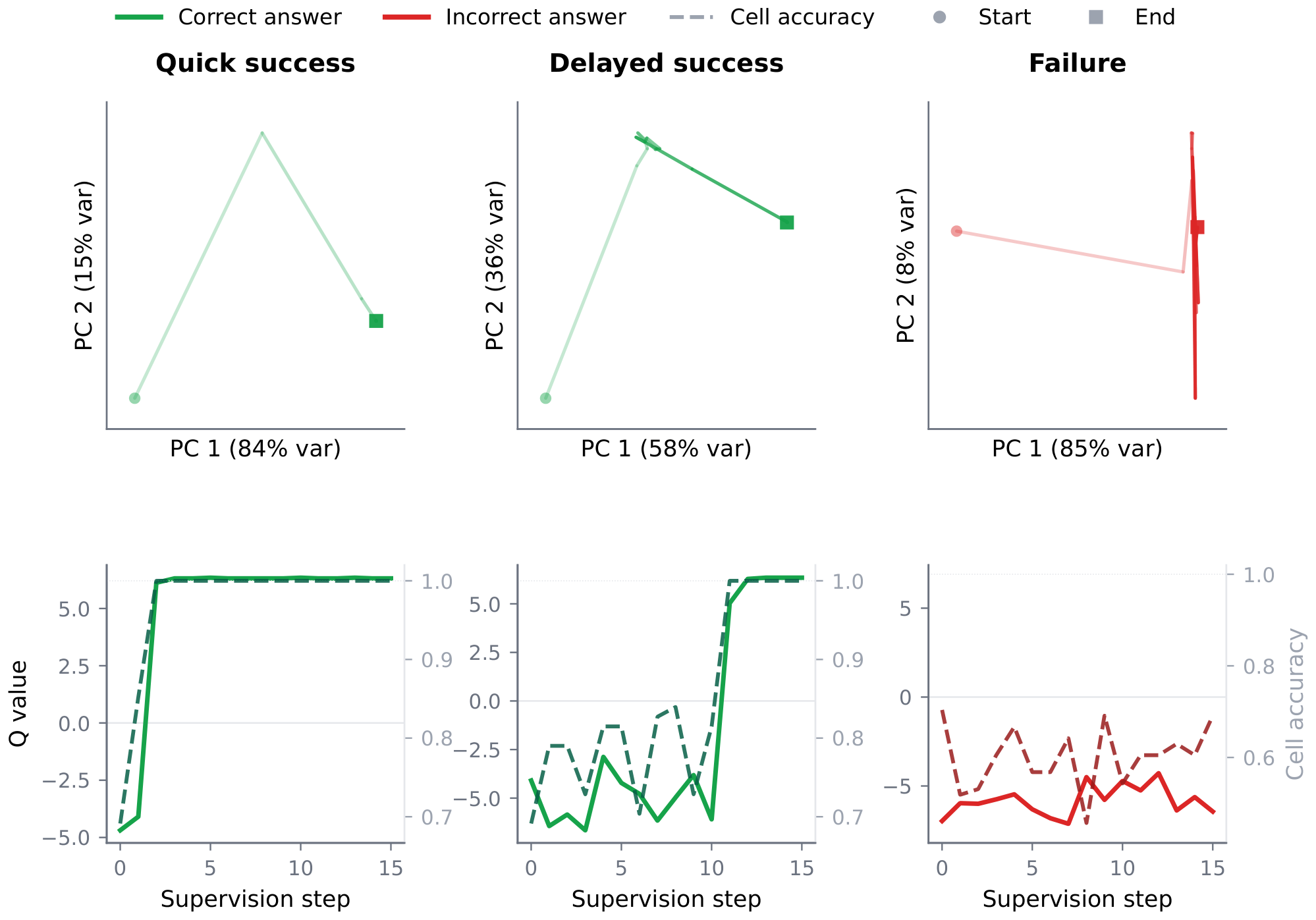
We present observations about TRM that motivate our method. In this section, we train a TRM on multiple Pencil Puzzle Bench (PPBench) ([8]) puzzles and inspect the latent dynamics and Q head behavior across supervision steps on a held-out validation set. For each puzzle, we record the latent $y_t$ and the Q logit $\hat{q}t = f_Q(y_t)$ at every supervision step $t = 1, \ldots, N\text{sup}$, project the latents into the principal plane (PCA per puzzle), and jointly plot the Q value alongside cell accuracy (fraction of correct cells in the predicted answer) over supervision steps. Figure 2 shows paired PCA and Q/cell-accuracy plots for three representative puzzles, illustrating three trajectory modes we observe:

Quick success: the trajectory transitions in a few steps from its starting location to a convergence region and remains there. Cell accuracy and the Q value rise together and saturate near their maxima within the same few steps.

Delayed success: the trajectory initially oscillates around one region and remains there for multiple supervision steps before sharply escaping to a different region where it converges. During the initial phase, the Q value is negative, and at the step where the trajectory escapes, both Q value and cell accuracy spike together.

Failure: the trajectory oscillates in a bounded region without converging. Cell accuracy never reaches near 100%, and the Q value stays negative for all supervision steps.

We refer to latent space regions that trajectories remain in across multiple supervision steps and exhibit similar cell accuracy throughout as basins. Basins where cell accuracy is near-maximal are good basins and basins where it is not are bad basins. Initially, failures and delayed successes behave similarly (both are caught in bad basins with negative Q). They diverge only later in their trajectories, when delayed successes find an escape to a good basin while failures remain stuck.

3.2 The Q head tracks trajectory quality

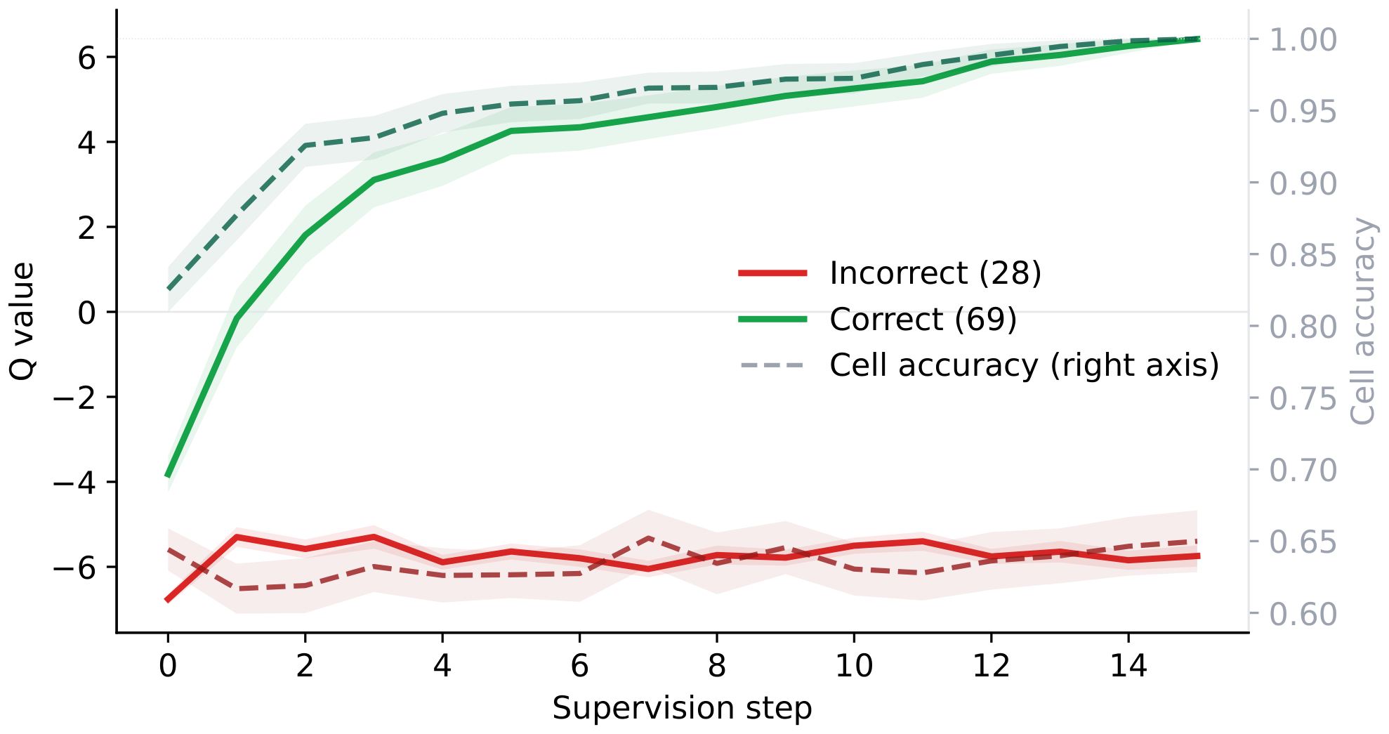
Across all three modes (failures, delayed successes, and quick successes), we find that the Q head's value closely tracks cell accuracy at every supervision step. To further confirm this, Figure 3 aggregates trajectories from 100 PPBench validation puzzles, separating them by final-answer correctness. The aggregate view corroborates the per-puzzle observation: mean Q and mean cell accuracy rise together on correct trajectories and remain mostly flat on incorrect ones. Moreover, at convergence, the Q logit sharply separates the two populations where q_hat approx +6\ (sigmoid

$ \approx 1 $

)$ for correct trajectories and $q_hat approx -6\ (sigmoid

$ \approx 0 $

) for incorrect ones. The Q head is therefore a reliable learned indicator of whether a trajectory has reached a good basin.

Given that the Q head's ability to distinguish good from bad trajectories, a natural question follows: can we leverage the Q head to identify better trajectories? The main challenge is that the standard TRM is inherently deterministic, and thus cannot be used to sample different trajectories for a given problem. In the next section, we will show that by simply adding Gaussian noise to the latent state, we can sample different parallel trajectories and leverage the Q head to pick the best one.

4. Method: Test-Time Compute Scaling via Stochastic Rollouts

Section Summary: The method introduces Probabilistic TRM, a simple inference procedure that adds random noise to any pretrained TRM model at each recursion step, runs multiple independent rollouts, and uses the model's existing Q head to pick the best final answer. This stochastic sampling lets some trajectories escape the dead-end regions of latent space that trap the usual deterministic version, while the number of rollouts provides a new, parallelizable way to spend extra test-time compute. Experiments show that scaling the number of rollouts steadily lifts accuracy, with the learned Q scorer reliably identifying correct solutions even when they are rare.

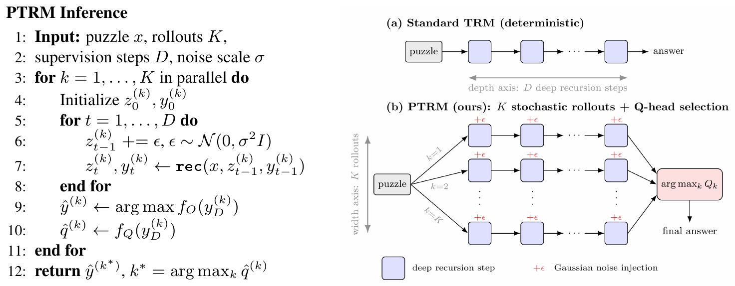
We propose Probabilistic TRM (PTRM), an inference-time procedure that makes the TRM recursion stochastic and selects the best of $K$ resulting trajectories. PTRM requires no special training and can be readily applied to any pretrained TRM model. Furthermore it requires no task-specific augmentations. PTRM works as follows: at each supervision step, we add Gaussian noise (scaled by $\sigma$) to the latent state input. The Q head $f_Q$ scores each candidate latent output, and the one with the highest Q value is selected and then decoded using the model's output head $f_O$. The algorithm in Figure 4 (left) states this formally. PTRM offers two complementary benefits: 1) it enables trajectories to escape bad basins where deterministic TRM remains stuck, and 2) it introduces width as a new axis for test-time scaling.

4.1 Escaping bad basins

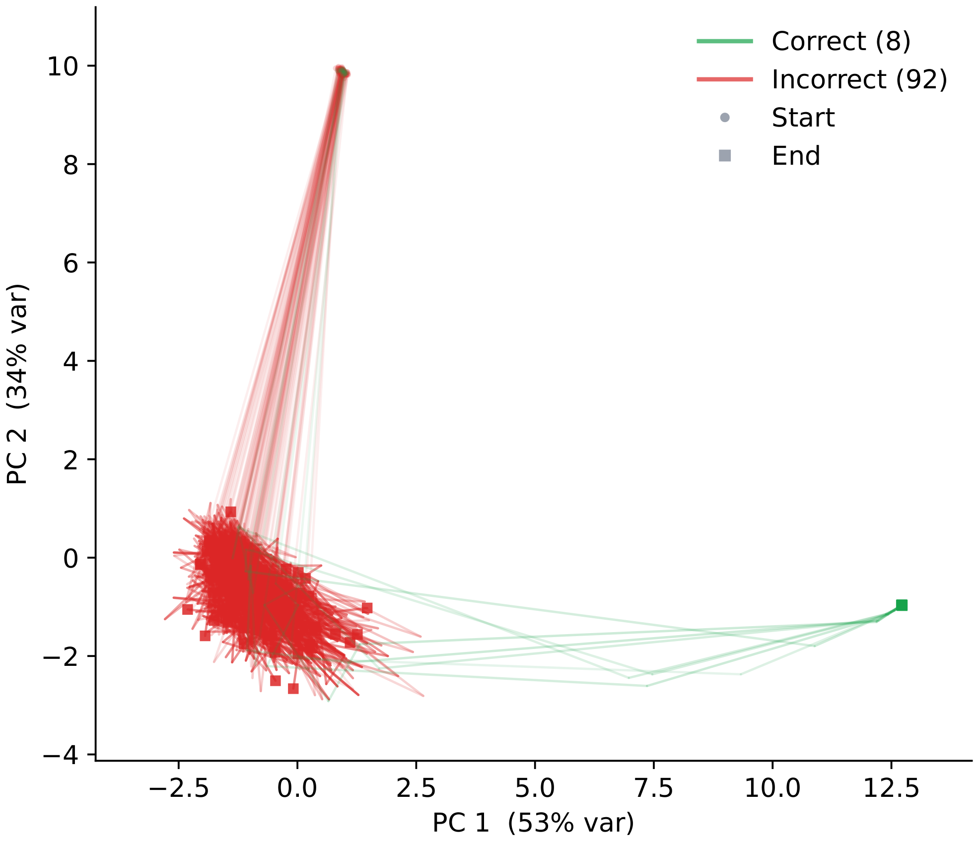
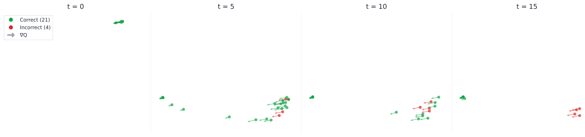
In Section 3, we found that some failed deterministic trajectories are caught in bad solution basins in latent space, with no way to escape. PTRM lets us test whether stochastic perturbations are enough for some of the rollouts of a previously failed puzzle to reach a good solution basin. Figure 5 shows K=100 independent rollouts, from the same failed puzzle used in Figure 2 (which fails at K=1), projected into the principal plane. Most rollouts (92%) remain stuck in the same bad basin, while a minority (8%) escape to a distinct region in latent space and produce correct answers. We also observe that recurrent noise creates a per-rollout probability of escape: at $K=5$ no rollouts escape, at $K=25$ one does, and at $K=100$ eight do. This confirms that noise provides the stochasticity needed to occasionally find an escape trajectory.

4.2 Width scaling

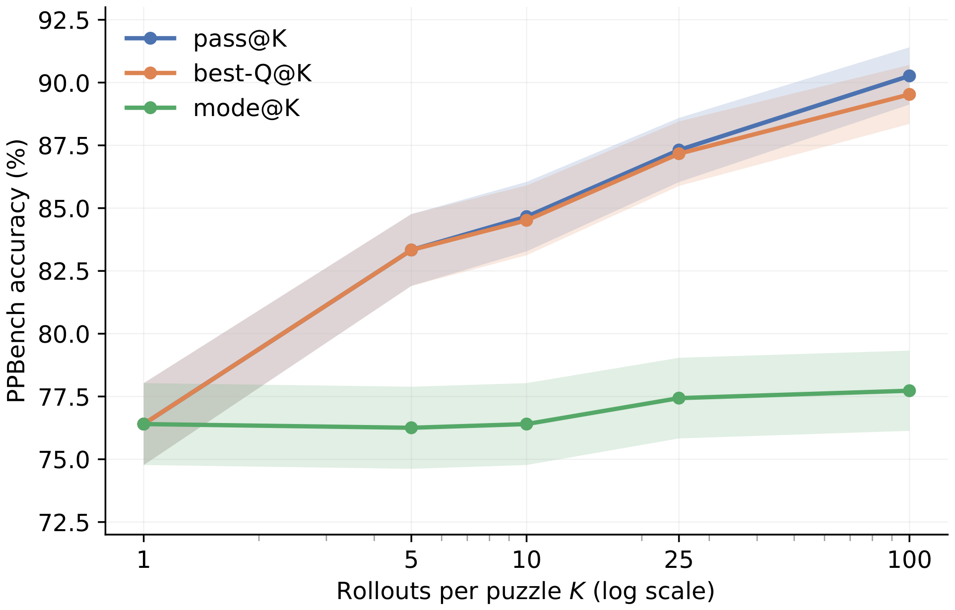
Since more rollouts per puzzle compound the chance that at least one reaches a good basin, the number of rollouts $K$ is a natural quantity to scale. Given $K$ independent rollouts, pass@K (any rollout correct) is the oracle upper bound and best-Q@K (the rollout with highest $\hat{q}$ is correct) is a metric available at inference without a correctness oracle. The choice of Q as selector is motivated by Section 3's observation that Q accurately separates correct from incorrect trajectories (Figure 3).

Figure 6 shows pass@K and best-Q@K as $K$ grows, averaged over 3 seeds on the held-out PPBench validation set (sudoku, nurikabe, tapa, lightup, and heyawake). Both metrics rise from 76.4% at $K=1$ to 89.5% at $K=100$, a gain of 13 percentage points. Across all tested K, the gap between pass@K and best-Q@K stays under 1pp, making the Q head a strong verifier on this validation set. By contrast, mode@K (most frequent answer across rollouts) rises by only 1.3pp over the same range, showing that the width-scaling gains come mostly from the Q head's ability to identify correct solutions even when they are rare.

Interaction with depth scaling. Depth is another scaling axis already supported by TRM, which consists of running more deep recursions (supervision steps) at inference than the $N_\text{sup}$ the model was trained on. On the deterministic baseline ($K$ =1), tripling the depth from 16 to 48 steps raises PPBench validation accuracy from 76.4% to 79.5% (+3.1pp). At higher $K$, depth scaling only provides additional gains on specific puzzle types such as sudoku (+4pp at $K=100$). Both depth and width scaling can be seen as ways to explore the model's solution space. Since rollouts are independent and parallelizable while extra depth is sequential, width is the more practical scaling axis.

PTRM unlocks a simple and task-agnostic recipe for scaling TRM test-time compute. The next section evaluates the method across multiple benchmarks and against several baselines, including frontier LLMs.

5. Experiments

Section Summary: The experiments section assesses how a method called PTRM improves reasoning performance on challenging puzzle benchmarks, including variants of pencil puzzles, Sudoku, mazes, and abstract reasoning tasks. It compares PTRM against a standard non-random version of the underlying model, simpler direct-prediction approaches, and leading large language models, using only extra computation at inference time rather than retraining. Results show large gains in accuracy over the baseline model on held-out test sets, with PTRM substantially outperforming both individual frontier models and an ensemble of them on the main puzzle collection while providing cost estimates for comparison.

This section evaluates PTRM's performance on diverse reasoning benchmarks. We compare against the deterministic TRM baseline, a non-recursive direct-prediction baseline, and frontier LLMs. Across several PPBench puzzles ([8]), Sudoku-Extreme ([2]), Maze-Hard ([2]), and ARC-AGI 2 ([4]), PTRM substantially boosts the performance of each pretrained TRM using only inference compute.

5.1 Setup

Datasets. Pencil Puzzle Bench (PPBench) ([8]) consists of 62, 231 constraint-satisfaction pencil puzzles (from 94 puzzle types). From the full PPBench dataset, 300 puzzles (15 puzzles from 20 types) selected by Waugh ([8]) are held out to form the golden set. From the remainder we hold out a fixed-size validation set of 100 puzzles per puzzle type (50 for tapa, due to its smaller base size), and the rest forms the training set. We filter all three sets to puzzles of six types (sudoku, lightup, nurikabe, shakashaka, heyawake, and tapa) of grid size 9 $\times$ 9 for sudoku, and 10 $\times$ 10 for the rest. We use the validation set to track performance during training and select the final checkpoint. We report per-puzzle accuracy on five of these types on the golden set (TRM already reaches 100% on shakashaka, so we omit it from the reported results), with aggregate scores sample-weighted across types. We also report results on the Sudoku-Extreme, Maze-Hard, and ARC-AGI 2 datasets.

Models and inference. For each benchmark we use a standard TRM checkpoint. For Sudoku-Extreme we use the TRM-MLP variant (which the TRM paper showed to be stronger on Sudoku), and for the other datasets, we use TRM-Att. PTRM inference uses $K$ parallel rollouts each running $D$ supervision steps with Gaussian noise of scale $\sigma$ added to the latent state at each supervision step. The selected configuration $(K, D, \sigma)$ varies by benchmark and is given alongside each result. Metrics are averaged across three seeds.

Baselines. To isolate the contribution of PTRM's stochastic rollouts from the underlying backbone, we report standard TRM performance (the same checkpoint as PTRM ran deterministically). For each dataset, we report the performance of frontier LLMs. For Sudoku-Extreme, Maze-Hard, and ARC2 we additionally report the published direct prediction and TRM baselines from ([1]).

Cost estimation. PPBench provides the dollar cost per attempt for each LLM. We convert PTRM's wall-clock to a comparable dollar figure using a single H100 at $2.50/hr (standard cloud pricing ([9])) so that $cost = $2.50 \cdot t_{\text{puzzle}} / 3600$, where $t_{\text{puzzle}}$ is the time (in seconds) to complete a puzzle.

5.2 Pencil Puzzle Bench

5.2.1 Per-puzzle accuracy

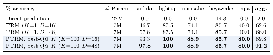
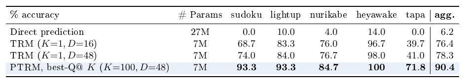
Table 1 reports per-puzzle accuracy on the PPBench golden set. PTRM at $K{=}100, D{=}48, \sigma{=}0.2$ raises aggregate best-Q@ $K$ from $62.6%$ to $91.2%$. Increasing supervision depth alone ($K{=}1, D{=}48$) gives a small boost over the standard TRM baseline ($K{=}1, D{=}16$). Most of the gain comes from scaling width (stochastic rollouts). The largest improvements are on puzzle types where the deterministic baseline performed the worst (most headroom): sudoku improves from $46.7%$ to $97.8%$ and tapa from $40.0%$ to $80.0%$.

::: {caption="Table 1: PPBench per-puzzle accuracy on the golden set. PTRM uses the same backbone as the deterministic TRM. Scaling depth alone (K=1, D=48) lifts aggregate accuracy by 3.4 points over the standard D=16 baseline. Combining depth with K=100 stochastic (sigma=0.2) rollouts raises accuracy by 28.6 percentage points overall. The direct-prediction baseline is a larger transformer trained on the same data."}

:::

5.2.2 Comparison with frontier LLMs on golden set

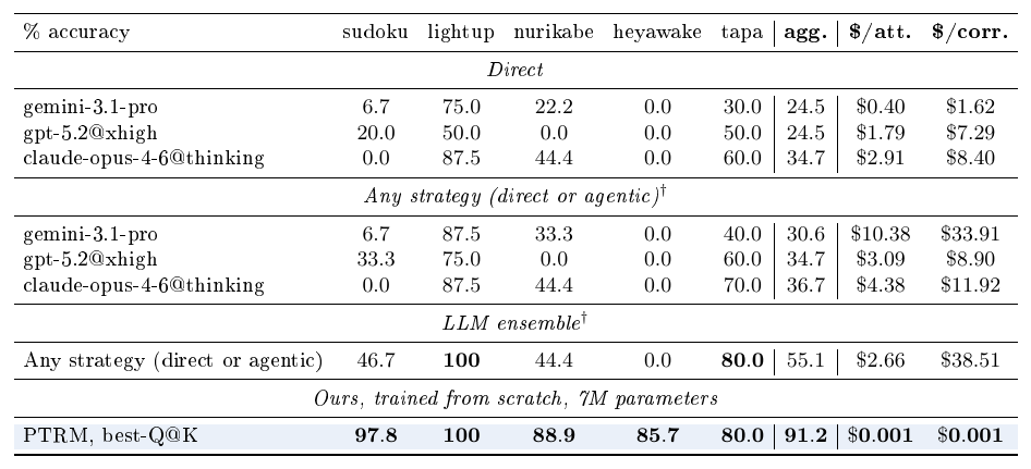
PPBench reported per-puzzle results for several frontier LLMs using two strategies: 1) direct response from a single prompt, and 2) multi-turn agentic strategy with verification. We report results for direct and any (best of any strategy attempted, including agentic). The agentic strategy gives the LLM substantially more resources than PTRM has access to. It provides the LLM the ability to iteratively verify each move with a perfect verifier. The direct strategy is the fairer comparison since, while it may use the model provider's reasoning harness, it does not have direct access to a multi-turn verifier (the LLM could still self-verify by writing verification code within the same response). We additionally observe that the agentic strategy was applied selectively in the published PPBench data: across the LLMs we compare against, only $9.6%$ of direct failures on the golden set were retried with agentic. We restrict the comparison to the 7 strongest LLMs that attempted every puzzle in our golden set: claude-opus-4-6@thinking, gpt-5.2@xhigh, gemini-3.1-pro, gpt-5.2@high, claude-sonnet-4-6@thinking, gpt-5.2@medium, and kimi-k2.5. Table 2 lists the top 3 in each strategy block.

We additionally report an ensemble score formed from these 7 LLMs where a puzzle counts as solved if at least one of them solved it via any strategy. This ensemble setup is deliberately stacked against PTRM. It assumes a perfect verifier since, if any of the 7 LLMs produced a correct answer under any strategy, the ensemble counts it as solved, even though in practice we would not have access to an oracle verifier. Although it is not deployable, we include the ensemble to demonstrate that even under these heavily favorable conditions, frontier LLMs fall well short of PTRM. Ensemble cost-per-attempt averages over the attempts of all 7 models on each puzzle, and cost-per-correct divides total cost by the number of puzzles the ensemble solved.

Table 2 reports the comparison. PTRM exceeds the strongest single LLM (direct strategy) by $57$ points aggregate ($91.2%$ vs. $34.7%$), and exceeds the LLM ensemble by $36$ points ($91.2%$ vs. $55.1%$) despite the ensemble's stacked advantages. Cost per attempt is several orders of magnitude higher for LLMs than PTRM.

::: {caption="Table 2: PTRM vs. frontier LLMs on PPBench golden. Per-puzzle accuracy and per-attempt / per-correct cost on the golden set. LLM costs are from PPBench. PTRM cost is estimated from H100 wall-clock (Section 5.1). The direct and agentic blocks list the 3 highest scoring LLMs on aggregate, and the ensemble row uses all 7 listed in Section 5.2.2. †Assumes access to a perfect verifier."}

:::

5.3 Sudoku-Extreme, Maze-Hard, and ARC-AGI-2

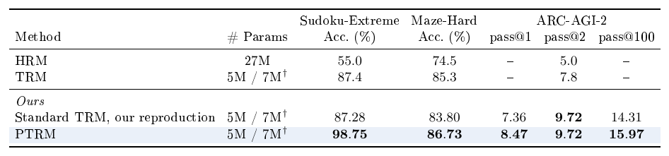
For each benchmark we use the standard TRM checkpoint trained as described in ([1]) without modification (TRM-MLP for Sudoku-Extreme and TRM-Att for Maze-Hard and ARC-AGI-2). Table 3 summarizes results on all three.

On Sudoku-Extreme, PTRM at $K{=}100, D{=}64, \sigma{=}0.3$ raises the deterministic baseline of $87.3%$ to $99.06%$ pass@ $K$ and $98.75%$ best-Q@ $K$, achieving state of the art.

On Maze-Hard, PTRM at $K{=}100$, $D{=}16$, $\sigma{=}1.0$ reaches $95.63%$ pass@ $K$, an $11.83$ point gain over the $83.8%$ deterministic baseline. mode@ $K$ gives the best PTRM accuracy here at $86.73%$ ($+2.93$ points), with best-Q@ $K$ slightly behind at $85.17%$ ($+1.37$ points). While pass@ $K$ shows that PTRM is able to unlock several correct answers, the Q head identifies them less reliably than on the previous benchmarks.

On ARC-AGI-2, the standard inference pipeline applies data augmentations and votes across them. PTRM adds $K$ stochastic rollouts per augmentation. For selection, we pick the rollout with the highest Q value within each augmentation, then vote across augmentations as in the standard pipeline. With $K{=}25$ and $\sigma{=}0.2$, PTRM lifts pass@1 from $7.36%$ to $8.47%$ and pass@100 from $14.31%$ to $15.97%$ over our deterministic TRM baseline, while matching it at pass@2.

::: {caption="Table 3: Sudoku-Extreme, Maze-Hard, and ARC-AGI-2 results. For Sudoku-Extreme, K=100, D=64, sigma=0.3. For Maze-Hard, K=100, D=16, sigma=1.0. For ARC-AGI-2, K=25, D=16, sigma=0.2. pass@ k for ARC-AGI-2 reports the top- k predictions from the augmentation-voting pipeline. PTRM shows an accuracy improvement over standard TRM across all 3 benchmarks. †Following ([1]), 5M for Sudoku-Extreme (TRM-MLP), 7M for Maze-Hard and ARC-AGI-2 (TRM-Att)."}

:::

5.4 Q head selection as $\sigma$ grows

With a higher $\sigma$ value, PTRM finds many correct solutions that the deterministic inference misses. For instance, on Maze-Hard, the deterministic model solves 83.8% of puzzles, but PTRM raises pass@ $K$ to nearly 96%. The extent to which PTRM helps depends on the task, but on every dataset we tested, it unlocks correct solutions well beyond the deterministic model's reach.

TRM's jointly trained Q head serves as a strong verifier on most tasks. On PPBench and Sudoku-Extreme, best-Q@ $K$ reaches values within a point of the saturated pass@ $K$, so PTRM's exploration translates directly into accuracy gains. On Maze-Hard, more exploration (higher $\sigma$) produces significantly more correct rollouts, but the existing Q head is not able to identify them, leaving performance on the table. The gap between best-Q@ $K$ and pass@ $K$ represents headroom for a stronger verifier which is left for future work. Appendix B reports the full $\sigma$ sweep.

6. Related Work

Section Summary: A substantial body of prior research has explored recursive neural networks that repeatedly refine their internal representations to tackle complex reasoning tasks, along with more recent approaches that perform this refinement in a continuous latent space rather than generating explicit text. Several of these studies introduce variations on noise injection or hidden-state reuse in models such as TRM, yet they typically require retraining, apply noise only once, or remain limited to narrow tasks. In contrast, the present work emphasizes a simpler, broadly applicable technique of adding noise at every step during inference, which avoids the more elaborate, task-specific remedies proposed in related analyses of attractor problems in similar architectures.

A long line of work explores recursive computation for iterative reasoning and representation refinement. Early examples include Universal Transformers ([10]), Mixture-of-Recursions ([11]), Deep Thinking models ([12, 13, 14]), and HRM ([2]), all of which investigate the use of repeated computation steps to improve reasoning performance. More recent work has introduced methods to substantially accelerate TRM training ([15]), while TRM-style recursive architectures have also been extended to language modeling tasks ([16]).

Building on this broader perspective of recursive computation, a growing body of work studies latent-space reasoning through the reuse of hidden states. [17] propose continuous “thinking tokens” derived from Chain-of-Thought (CoT) traces ([18]), which are autoregressively generated and appended to the model context, enabling reasoning directly in latent space without producing intermediate textual outputs. Similarly, [19] formalize learning by superposition and demonstrate improvements on tasks such as graph reachability. By avoiding explicit token sampling and implicitly representing multiple reasoning trajectories, these approaches may mitigate the unfaithfulness and backtracking often observed in standard autoregressive reasoning ([20, 21]).

Related to our work, [22] propose a generative version of TRM where the hidden state $z$ is sampled instead of deterministic. This improves performance on multiple tasks, but requires retraining. [23] (concurrent work) propose a similar test-time compute method where they only apply noise in the initial hidden state $z$, while we apply noise at every supervision step. Furthermore, they test their method on a small subset of the Sudoku-Extreme dataset, and treat it as a proof-of-concept that needs to be developed and tested further. Note that [22] also tested applying noise to the initial $z$ with TRM and obtained negative results (no improvement in accuracy on two datasets).

Our observations in Section 3 are consistent with the mechanistic analysis of [5], who identify spurious fixed points in HRM’s latent dynamics on Sudoku-Extreme. Their method mitigates these attractors through a combination of task-specific training data augmentation, inference-time input perturbations, and model bootstrapping across training checkpoints, thereby effectively increasing test-time compute. However, these interventions are comparatively less general and less computationally efficient. In contrast, we observe analogous basin structure in TRM across multiple puzzle types and achieve attractor escape using a substantially simpler, task-agnostic mechanism: injecting Gaussian noise into the latent state at each supervision step while using a single deterministic checkpoint.

7. Conclusion

Section Summary: In this work, researchers introduced Probabilistic TRM, a simple add-on for tiny recursive models that improves performance by running many solution attempts in parallel at test time and then selecting the best one. The method requires no retraining, works across a range of logic puzzles, and reaches much higher accuracy than ensembles of large language models at a tiny fraction of the cost. The authors also note that gains vary by puzzle type and call for better ways to verify answers on harder problems.

In this work, we introduced Probabilistic TRM (PTRM), a novel test-time scaling paradigm for Tiny Recursive Models (TRM) through parallel exploration and selection. This approach scales test-time compute using width ($K$ parallel rollouts), yielding substantially larger gains than depth scaling (increasing deep recursion steps) alone. PTRM requires no retraining and does not rely on task-specific data augmentations making it extremely easy to use and versatile.

By scaling both width and depth, PTRM obtains significant gains in accuracy when tested on a wide selection of puzzles. On PPBench (Sudoku, Lightup, Nurikabe, Heyawake, Tapa puzzles), PTRM nearly obtains twice the accuracy ($91.2%$; $0.001$ cost) of ensemble of SOTA LLMs ($55.1%$; $38.51$ cost) at less than $0.0001$ x the cost. Furthermore, PTRM improves accuracy on Sudoku (from $87.4%$ to $98.75%$), Maze-Hard (from $83.80%$ to $86.73%$), and ARC-AGI (from $7.8%$ to $8.47%$ pass@1).

Limitations. Our experiments focus on reasoning puzzles rather than general tasks. We only test on a subset of PPBench puzzles. We are limited to puzzles with a small grid-size due to limited computational resources. It is not guaranteed that the method works as well for all types of problems (e.g., accuracy gains on ARC-AGI-2 and Heyawake are smaller).

Future work. It would be interesting to understand why some puzzles benefit from test-time scaling more than others. We suspect that problems that are harder to verify (e.g., ARC-AGI-2) benefit less from PTRM because the Q head may struggle to distinguish correct solutions from incorrect ones. Developing stronger verifiers than the existing Q head is an interesting direction for future work.

Appendix

Section Summary: The appendix outlines the practical setup for training models on a single high-end GPU using existing architectures with no added computational cost, along with the construction of a puzzle dataset drawn from thousands of constraint-satisfaction examples that were filtered, split into training/validation/test sets, and expanded via random transformations and partial solution states. It also presents experiments showing how varying levels of inference noise improve the rate of discovering correct solutions across tasks, with performance curves for different selection methods. Finally, it notes a negative result where an attempted gradient-based sampling method added nothing beyond basic noise injection.

A. Implementation Details

A.1 Compute

We train and evaluate all models on a single NVIDIA H100 80GB GPU. PTRM introduces no additional training cost over standard TRM since it operates entirely at inference time.

A.2 Models

All experiments use the standard TRM backbone ([1]) with the released architecture and training recipes. Following the TRM paper, we use the MLP variant (TRM-MLP, 5M parameters) for Sudoku-Extreme and the attention variant (TRM-Att, 7M parameters) for Maze-Hard, ARC-AGI-2, and PPBench. Layout and hyperparameters are unchanged from TRM.

A.3 PPBench dataset construction

Sudoku-Extreme, Maze-Hard, and ARC-AGI-2 use the same checkpoints and data splits as TRM. The PPBench dataset is more recent and has previously been used only with frontier LLMs, so we detail how we built our training, validation, and golden splits.

Source.

PPBench contains $62{,}231$ constraint-satisfaction pencil puzzles spanning 94 puzzle types. Of these, 300 puzzles ($15$ puzzles $\times$ $20$ types) are held out as the golden benchmark set by Waugh ([8]).

Filtering.

From the remaining $61{,}931$ puzzles we hold out a validation set by sampling 100 puzzles from each puzzle type (50 for tapa, due to its smaller base size), and the rest forms the training set. We then filter all three sets (training, validation, golden) to retain only puzzles of six types (sudoku, lightup, nurikabe, shakashaka, heyawake, tapa) at fixed grid sizes: $9{\times}9$ for sudoku and $10{\times}10$ for the others. Sudoku grids are padded with a pad token to $10{\times}10$, giving a uniform sequence length of $\text{seq_len}=100$ across all six puzzle types. The deterministic TRM baseline reaches 100% accuracy on shakashaka, so we exclude it from per-puzzle accuracy reporting (no headroom to compare against PTRM).

Augmentation.

Each training puzzle is expanded into 10 examples using two augmentations: 1) trajectory sampling, where the input is set to a random intermediate solve state along the puzzle's solution trajectory rather than always the empty initial grid, while the label is always the fully solved grid; and 2) dihedral transformation, where a random dihedral transformation of a square grid, among the 8 possibilities given by 4 rotations $\times$ 2 identity, reflection, is applied to both the input and the label. For each puzzle, the first example is the unaugmented (initial state, solved) pair. The remaining 9 are randomly sampled (trajectory and dihedral transform). Validation and golden splits are not augmented.

Resulting splits.

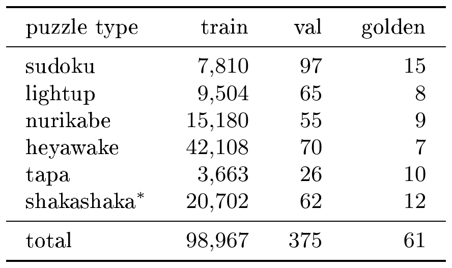
The merged multi-type splits use a unified vocabulary of 294 tokens and $\text{seq_len}=100$. Per-type sample counts are reported in Table 4.

::: {caption="Table 4: Per-puzzle-type sample counts in the PPBench splits used in training and evaluation. *Shakashaka is included in training but excluded from per-puzzle accuracy reporting because deterministic TRM already solves all evaluated shakashaka puzzles."}

:::

B. Noise Ablation

We ablate the inference noise level $\sigma$ on three benchmarks at $K{=}25$ ($K{=}100$ for Maze-Hard) and $D{=}16$ to keep the sweep tractable. For Sudoku-Extreme we randomly sample 1000 puzzles from the test set for the same reason. Figure 7 shows pass@ $K$, best-Q@ $K$, and mode@ $K$ as a function of $\sigma$, averaged over three random seeds.

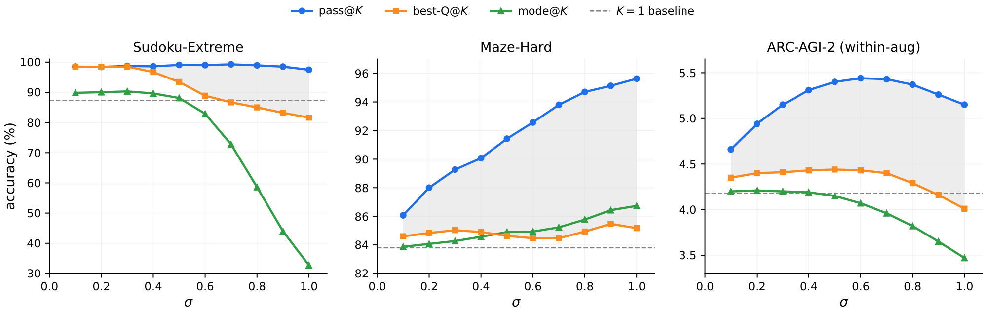
On Maze-Hard pass@ $K$ climbs from 83.8% (deterministic) to nearly 96% by $\sigma{\approx}1.0$ and then plateaus. On Sudoku-Extreme it is already near its ceiling at $\sigma{=}0.1$ and stays roughly flat across the sweep. On ARC-AGI-2 it peaks near $\sigma{=}0.6$ before declining. Q head selection nearly matches the ceiling (maximum pass@ $K$) on Sudoku-Extreme while best-Q@ $K$ peaks at $98.5%$ (within a point of pass@ $K$ 's peak of $99.3%$). On the other hand, the gap between best-Q@ $K$ and maximum pass@ $K$ is more pronounced on Maze-Hard and ARC-AGI-2 (headroom a stronger verifier could close).

C. Q-guided Langevin sampling

We initially explored Langevin sampling (using the Q head gradient) as a more principled exploration mechanism than the Gaussian noise injection used in PTRM. The idea is to better guide the stochastic search by additionally steering each rollout (using the Q head gradient) toward regions of high Q value. We ultimately found that the gain from this approach was entirely attributable to the Langevin noise term, with the gradient component contributing nothing measurable on top of the equivalent recurrent noise of Section 4. We document the approach here as a negative result.

Motivation.

The Q head is trained as a correctness predictor over latent states. Let $f_Q(z)$ denote the head's scalar output. We treated $E(z) = -\log \mathrm{sigmoid}(f_Q(z))$ as an energy function over latent space. Empirical observations during early experiments suggested that regions of low $E$ correspond to good basins from which the decoded answer is likely correct. PCA visualizations of the latent dynamics showed that $\nabla_z f_Q$ points toward the good-basin region from both good-basin (correct) and bad-basin (incorrect) latents (Figure 8). This made $\nabla_z f_Q$ look like a valuable direction along which to push latents.

Method.

We sample from the target distribution $p(z) \propto e^{-E(z)} = \mathrm{sigmoid}(f_Q(z))$ via Langevin dynamics where at the end of each deep recursion step $t = 1, \ldots, D$ we apply $N$ Langevin steps to the latent,

$ z \leftarrow z - \eta, \nabla_z E(z) + \sqrt{2\eta}, \xi, \quad \xi \sim \mathcal{N}(0, I), $

The number of Langevin steps $N$ is the additional scaling axis under this scheme.

Tractable gradient computation.

TRM's original Q head is a linear projection on a single token, $f_Q(y) = w^\top y[:, 0] + b$, so its gradient with respect to this head's input is a constant vector independent of $z$. For $\nabla_z f_Q$ to be input-dependent, the gradient must flow back through the last latent recursion. This works but requires backpropagating through a full latent recursion at every Langevin step, which scales poorly with $N$. To make guidance tractable for large $N$, we replaced the linear Q head with an attention-pooled variant that reads the full latent and produces a scalar through a small nonlinear network. With this head, $\nabla_z f_Q$ can be computed by backpropagating through the head alone, which is $\sim$ 8 $\times$ faster per step and does not sacrifice accuracy.

The gain came from the noise, not the gradient.

Comparing Langevin sampling against a noise-only ablation (with the same $\sqrt{2\eta}, \xi$, but with the $-\eta, \nabla_z E(z)$ term zeroed out) produced essentially identical accuracy at matched $N$. The gradient component contributed nothing measurable on top of the equivalent recurrent noise. This prompted us to focus on the noise-only formulation in Section 4, which is much more impactful since it is: 1) significantly simpler (no retraining, no test-time backpropagation), 2) applicable to any TRM checkpoint out of the box, and 3) equally effective.

D. Per-puzzle accuracy on the PPBench validation set

The main paper reports per-puzzle accuracy on the PPBench golden set (Table 1) for direct comparability with the LLM evaluations from Waugh ([8]) who used that set. For a lower-variance complement, Table 5 reports results on our validation set ($313$ puzzles across the five reported types vs. $49$ for golden). Trends match the golden-set results: depth scaling alone ($K{=}1, D{=}48$) provides a small lift, and combining depth with stochastic rollouts ($K{=}100, D{=}48, \sigma{=}0.2$) raises aggregate best-Q@ $K$ from $76.4%$ to $90.4%$, a $14.0$ percentage-point improvement. The biggest gains again are on puzzles where the deterministic baseline has the most headroom (tapa $\sim40%$ to $71.8%$, sudoku $\sim69%$ to $93.3%$). Types where the baseline is already near ceiling (heyawake at $96.7%$) increase only marginally.

::: {caption="Table 5: PPBench per-puzzle accuracy on the validation set. PTRM uses the same backbone as the deterministic TRM. Results on the larger validation set follow the same trends as on the golden set."}

:::

References

Section Summary: This references section compiles a list of research papers, preprints, and workshop contributions mainly exploring reasoning mechanisms in artificial intelligence, such as recursive neural networks, chain-of-thought prompting, and hierarchical models for solving complex problems. The works span from foundational pieces in 2016 to recent 2025–2026 studies on scaling computation, measuring true reasoning versus pattern guessing, and developing new benchmarks like ARC-AGI. It also includes one practical resource on accessing GPU hardware for experiments.

[1] Jolicoeur-Martineau, Alexia (2025). Less is more: Recursive reasoning with tiny networks. arXiv preprint arXiv:2510.04871.

[2] Wang et al. (2025). Hierarchical Reasoning Model. arXiv preprint arXiv:2506.21734.

[3] Chollet, François (2019). On the measure of intelligence. arXiv preprint arXiv:1911.01547.

[4] Chollet et al. (2025). Arc-agi-2: A new challenge for frontier ai reasoning systems. arXiv preprint arXiv:2505.11831.

[5] Ren, Zirui and Liu, Ziming (2026). Are Your Reasoning Models Reasoning or Guessing? A Mechanistic Analysis of Hierarchical Reasoning Models. arXiv preprint arXiv:2601.10679.

[6] Snell et al. (2024). Scaling llm test-time compute optimally can be more effective than scaling model parameters. arXiv preprint arXiv:2408.03314.

[7] Graves, Alex (2016). Adaptive computation time for recurrent neural networks. arXiv preprint arXiv:1603.08983.

[8] Waugh, Justin (2026). Pencil Puzzle Bench: A Benchmark for Multi-Step Verifiable Reasoning. arXiv preprint arXiv:2603.02119.

[9] Vast.ai (2026). Rent H100 PCIE GPUs on Vast.ai. https://vast.ai/pricing/gpu/H100-PCIE. Accessed: 2026-05-01.

[10] Dehghani et al. (2018). Universal transformers. arXiv preprint arXiv:1807.03819.

[11] Bae et al. (2025). Mixture-of-recursions: Learning dynamic recursive depths for adaptive token-level computation. arXiv preprint arXiv:2507.10524.

[12] Schwarzschild et al. (2021). Can you learn an algorithm? generalizing from easy to hard problems with recurrent networks. Advances in Neural Information Processing Systems. 34. pp. 6695–6706.

[13] Bansal et al. (2022). End-to-end algorithm synthesis with recurrent networks: Extrapolation without overthinking. Advances in Neural Information Processing Systems. 35. pp. 20232–20242.

[14] Bear et al. (2024). Rethinking Deep Thinking: Stable Learning of Algorithms using Lipschitz Constraints. Advances in Neural Information Processing Systems. 37. pp. 97027–97052.

[15] Hakimi, Navid (2026). Form Follows Function: Recursive Stem Model. arXiv preprint arXiv:2603.15641.

[16] Li et al. (2026). Learning Multi-step Reasoning via Persistent Latent State Propagation. In Workshop on Latent & Implicit Thinking – Going Beyond CoT Reasoning.

[17] Hao et al. (2024). Training large language models to reason in a continuous latent space. arXiv preprint arXiv:2412.06769.

[18] Wei et al. (2022). Chain-of-thought prompting elicits reasoning in large language models. Advances in neural information processing systems. 35. pp. 24824–24837.

[19] Zhu et al. (2025). Reasoning by Superposition: A Theoretical Perspective on Chain of Continuous Thought. arXiv preprint arXiv:2505.12514.

[20] Lanham et al. (2023). Measuring faithfulness in chain-of-thought reasoning. arXiv preprint arXiv:2307.13702.

[21] Chen et al. (2025). Reasoning Models Don't Always Say What They Think. arXiv preprint arXiv:2505.05410.

[22] Baek et al. (2026). Generative Recursive Reasoning Models. ICLR 2026 Workshop on AI with Recursive Self-Improvement.

[23] Efstathiou, Andreas and Balwani, Aishwarya (2026). Recursive Reasoning as Attractor Landscape Search: Mechanistic Dynamics of the Tiny Recursive Model. Workshop on Latent & Implicit Thinking – Going Beyond CoT Reasoning. https://openreview.net/forum?id=kKps9W1K7n.