Extending the Context of Pretrained LLMs by Dropping Their Positional Embeddings

Show me an executive summary.

Purpose and context

Language models based on transformers struggle when asked to process sequences longer than those seen during training. The main culprit is the way these models encode position information using rotary positional embeddings (RoPE). While RoPE helps models learn effectively during training, it prevents them from generalizing to longer contexts without expensive additional fine-tuning on long sequences. This work investigates whether positional embeddings can be removed after training to unlock zero-shot generalization to much longer contexts, while preserving performance on the original training context.

What was done

The researchers developed DroPE (Dropping Positional Embeddings), a method that removes all positional embeddings from a pretrained language model after most training is complete. The approach involves three phases: (1) train a model normally with RoPE for most of the training budget, (2) remove the positional embeddings, and (3) continue training briefly (a "recalibration phase") at the original context length to let the model adapt. They tested DroPE on models ranging from 360 million to 7 billion parameters, trained on datasets from 16 billion to 4 trillion tokens. Evaluations focused on in-context performance on standard benchmarks and zero-shot performance on sequences up to 16 times longer than the training context, using needle-in-a-haystack retrieval tasks and long-context question answering.

Main findings

DroPE enables pretrained models to generalize zero-shot to contexts far beyond their training length without any long-context fine-tuning. On needle-in-a-haystack tests at twice the training context, DroPE achieved 28-42% success rates compared to 0-22% for baseline methods including standard RoPE scaling techniques. On challenging long-context benchmarks, DroPE improved average scores by over 10 times compared to the base model and outperformed all RoPE-scaling baselines. Critically, DroPE preserves the original model's performance on standard in-context tasks, matching or slightly exceeding baseline scores across reasoning and question-answering benchmarks. The recalibration phase is remarkably efficient: models recover over 95% of original performance after less than 1% of the original training budget.

Why these results matter

Current methods for extending context require costly fine-tuning on long sequences, which is computationally prohibitive at the scale of modern foundation models. DroPE eliminates this bottleneck entirely. The method can be integrated into standard training pipelines at essentially zero extra cost by simply dropping positional embeddings near the end of pretraining. More importantly, DroPE can be applied to any existing pretrained model in the wild with minimal additional training, making long-context capabilities accessible without retraining from scratch. The findings challenge the conventional assumption that positional embeddings are necessary throughout a model's lifecycle, revealing they function primarily as a training aid rather than a permanent architectural requirement.

Recommendations and next steps

Training teams should consider integrating DroPE into their standard pipelines by removing positional embeddings in the final 10-15% of training. For organizations with existing pretrained models, applying DroPE through brief recalibration (1-2% of original training tokens) offers an efficient path to long-context capabilities. The main trade-off is a short additional training phase, but this is negligible compared to the cost of long-context fine-tuning or retraining. Before deploying DroPE models in production, teams should validate performance on their specific downstream tasks, though results across multiple benchmarks suggest risks are low. Future work should explore optimal recalibration schedules for different model sizes and investigate whether similar principles apply to other architectural components.

Limitations and confidence

The largest models tested were 7 billion parameters, so behavior at frontier model scale (hundreds of billions of parameters) remains uncertain, though trends across tested scales are consistent. The method requires choosing when to start recalibration and how long to continue; while guidelines are provided, optimal settings may vary by use case. Results are based on specific tokenizers and architectures (Qwen, Llama, SmolLM families); generalization to other architectures should be verified. The confidence in core findings is high: results replicate across different model sizes, datasets, and evaluation tasks. The main uncertainty is how performance scales beyond 16 times the training context, which was the maximum tested extension factor.

Yoav Gelberg

^{1,2}

, Koshi Eguchi

^{1}

, Takuya Akiba

^{1}

and Edoardo Cetin

^{1}

^{1}

Sakana AI

^{2}

University of Oxford

Correspondence: Yoav Gelberg ([email protected]), Edoardo Cetin ([email protected])

Abstract

So far, expensive finetuning beyond the pretraining sequence length has been a requirement for effectively extending the context of language models (LM). In this work, we break this key bottleneck by Dropping the Positional Embeddings of LMs after training (DroPE). Our simple method is motivated by three key theoretical and empirical observations. First, positional embeddings (PEs) serve a crucial role during pretraining, providing an important inductive bias that significantly facilitates convergence. Second, over-reliance on this explicit positional information is also precisely what prevents test-time generalization to sequences of unseen length, even when using popular PE-scaling methods. Third, positional embeddings are not an inherent requirement of effective language modeling and can be safely removed after pretraining following a short recalibration phase. Empirically, DroPE yields seamless zero-shot context extension without any long-context finetuning, quickly adapting pretrained LMs without compromising their capabilities in the original training context. Our findings hold across different models and dataset sizes, far outperforming previous specialized architectures and established rotary positional embedding scaling methods.

Code https://github.com/SakanaAI/DroPE

1. Introduction

Show me a brief summary.

In this section, the authors address the computational intractability of pretraining transformer language models on long sequences due to quadratic attention costs, which has made zero-shot context extension—enabling models to handle sequences beyond their training length without additional finetuning—a central challenge. While popular rotary positional embedding (RoPE) scaling techniques attempt to adapt models to longer contexts, they fail to generalize effectively without expensive long-context finetuning, and alternative architectures introduce performance trade-offs that limit adoption. The authors propose DroPE (Dropping Positional Embeddings), which removes positional embeddings after pretraining following a short recalibration phase at the original context length. This method is motivated by three key observations: positional embeddings accelerate pretraining convergence, over-reliance on them prevents length generalization, and they can be safely removed post-training. DroPE achieves seamless zero-shot context extension without long-context finetuning, outperforming RoPE-scaling methods while preserving in-context capabilities across models up to 7B parameters.

Transformers established themselves as the predominant architecture for training foundation models at unprecedented scale in language and beyond ([1, 2, 3, 4]). The defining feature of transformers is abandoning explicit architectural biases such as convolutions and recurrences in favor of highly general self-attention layers ([5]), while injecting positional information about the sequence through positional embeddings (PEs) and causal masking. However, despite significant efforts to scale attention to long sequences on modern hardware ([6, 7, 8]), this powerful layer is inherently bottlenecked by quadratic token-to-token operations, which makes pretraining at long sequence lengths computationally intractable at scale. As a result, enabling models to use contexts beyond their pretraining length without additional long-context fine-tuning (i.e., "zero-shot context extension") has emerged as a central challenge for the next generation of foundation models ([9, 10]).

When inference sequence lengths exceed the pretraining context, the performance of modern transformer-based LMs degrades sharply. This is directly caused by their use of explicit PEs such as the ubiquitous rotary positional embeddings (RoPE) ([11]), which become out-of-distribution at unseen sequence lengths. To address this issue, careful scaling techniques that adapt RoPE frequencies on longer sequences were introduced ([12, 13, 14, 15]). However, despite their popularity, these methods still rely on an expensive, long-context finetuning phase to meaningfully use tokens beyond the original sequence length, failing to generalize out of the box ([16]). Beyond RoPE transformers, alternative architectures and positional embedding schemes have shown early promise in reducing costs by attenuating the underlying quadratic computational burden [17, 18, 19, 20] or maintaining better out-of-context generalization ([21, 22, 23]). Yet, these parallel efforts are still far from challenging established pipelines, introducing notable performance and stability trade-offs that prevent wide adoption.

In this work, we challenge the conventional role of RoPE in language modeling, and propose to overcome this inherent trade-off by Dropping the Positional Embeddings (DroPE) of LMs after pretraining. Our method is based on three key theoretical and empirical observations. First, explicit positional embeddings significantly facilitate pretraining convergence by baking in an important inductive bias that is difficult to recover from data alone. Second, over-reliance on positional embeddings is precisely what prevents test-time generalization to sequences of unseen length, with RoPE-scaling context extension methods focusing on recent tokens instead of ones deeper in the context to retain perplexity. Third, explicit PE is not an inherent requirement for effective language modeling and can be removed after pretraining, following a short recalibration phase which is performed at the original context length.

Empirically, DroPE models generalize zero-shot to sequences far beyond their training context, marking a sharp contrast to traditional positional scaling techniques. Moreover, we show that adapting RoPE models with DroPE does not compromise their original in-context capabilities, preserving both perplexity and downstream task performance. Our findings hold across LMs of different architectures and sizes up to 7B parameters pretrained on trillions of tokens, establishing a new standard for developing robust and scalable long-context transformers.

Contributions. In summary, our main contributions are as follows:

In Section 3, we provide empirical and theoretical analysis of the role of positional embeddings in LM training, showing their importance in significantly accelerating convergence.
In Section 4, we discuss why RoPE-scaling methods fail to reliably attend across far-away tokens when evaluated zero-shot on long sequences, showing that these approaches inevitably shift attention weights, hindering the model's test-time behavior.
In Section 5, we introduce DroPE, a new method that challenges the conventional role of positional embeddings in transformers, motivated by our empirical and theoretical analyses of its role as a transient but critical training inductive bias.
We demonstrate that DroPE enables zero-shot generalization of pretrained RoPE transformers far beyond their original sequence length, without any long-context finetuning. DroPE can be incorporated at no extra cost into established training pipelines, and can be used to inexpensively empower arbitrary pretrained LLMs in the wild.

We share our code to facilitate future work and extensions toward developing foundation models capable of handling orders-of-magnitude longer contexts.

2. Preliminaries

Show me a brief summary.

In this section, the fundamental mechanisms of transformer-based language models are established, focusing on how positional information is incorporated during training. Self-attention computes weighted combinations of value vectors based on query-key similarity scores, but lacks inherent awareness of token order. To address this, modern transformers use Rotary Positional Embeddings (RoPE), which encode relative positions by rotating query and key vectors with frequency-dependent angles before computing attention scores. When deploying these models on sequences longer than their training context, RoPE becomes out-of-distribution, necessitating frequency scaling methods like PI, RoPE-NTK, and YaRN that adjust rotational frequencies to accommodate extended contexts. However, these scaling techniques still require expensive long-context finetuning and fail to generalize zero-shot to downstream tasks. An alternative approach, NoPE transformers, eliminates positional embeddings entirely but suffers from degraded performance compared to RoPE architectures, preventing widespread adoption despite avoiding the need for frequency rescaling.

Self-attention. Let

h1,…,hT∈Rdh_1, \dots, h_T\in {\mathbb{R}}^{d}

be the representations fed into a multi-head attention block. Queries

q_i

, keys

k_i

, and values

v_i

are computed by projecting the inputs

h_i

via linear layers

W_Q

W_K

, and

W_V

. The attention operation then computes a

\times T

matrix of attention scores

s_{ij}

and then weights

αij\alpha_{ij}

between all pairs of sequence positions, and reweighs value vectors:

where

d_k

is the head dimension. A multi-head attention block computes multiple attention outputs

zi(1),…,zi(H)z_i^{(1)}, \dots, z_i^{(H)}

, concatenates them, and projects to the model dimension:

oi=WO[zi(1),…,zi(H)]o_i = W_O[z_i^{(1)}, \dots, z_i^{(H)}]

Language and positional embeddings. State-of-the-art autoregressive transformer LMs use information about sequence positions provided both implicitly via causal masking of the attention scores¹, and explicitly with positional embeddings. In particular, the modern literature has settled on the Rotary PE (RoPE) scheme ([11]), providing relative positional information to each attention head by rotating

q_i

and

k_j

in 2D chunks before the inner product in Equation 1:

Note the softmax in Equation 1 is taken on the first

i

tokens, implementing a causal mask.

Here, each

R(ωm)∈R2×2R(\omega_m)\in \mathbb{R}^{2\times2}

is a planar rotation of angle

ωm=b−2(m−1)/dk\omega_m=b^{-2(m-1)/d_k}

acting on the

(2 m, 2 m + 1)

subspace of

q_i

and

k_j

. The base

b

is commonly taken to be

10{, }000

Context extension for RoPE. Given the rapidly growing costs of self-attention, adapting LMs for longer sequences than those seen during training has been a longstanding open problem. To this end, prior context-extension methods introduce targeted rescaling of the RoPE frequencies in Equation 2 to avoid incurring unseen rotations for new sequence positions. Formally, let the training and inference context lengths be

Ctrain<CtestC_\mathrm{train} < C_\mathrm{test}

, and define the extension factor

C_\mathrm{test} / C_\mathrm{train}

. Context extension methods such as PI ([12]), RoPE-NTK ([13]), and the popular YaRN ([14]) define new RoPE frequencies

ωm′=γmωm\omega_m' = \gamma_m \omega_m

with scaling factors:

where

κm∈[0,1]\kappa_m \in [0, 1]

interpolates between 0 and 1 as the base frequency

ωm\omega_m

grows (see Appendix A). These methods, referred to as RoPE-scaling, still require additional finetuning on long sequences, and don't generalize to long-context downstream tasks out of the box ([24]).

NoPE transformers. In a parallel line of work, there have been efforts to train transformers without PEs, commonly referred to as NoPE architectures ([25, 21]), to avoid the need for rescaling RoPE frequencies. While NoPE was shown to be a viable LM architecture, it has failed to gain traction due to degraded performance ([25, 22]) compared to RoPE architectures. For an in-depth introduction to the above concepts, see Appendix A.

3. Explicit positional embeddings are beneficial for training

Show me a brief summary.

In this section, the authors investigate why NoPE transformers consistently underperform RoPE architectures during training despite being theoretically expressive enough for sequence modeling. While NoPE transformers can encode positional information through causal masking alone, they develop positional bias and attention non-uniformity at a bounded, slower rate compared to RoPE models. The analysis introduces the concept of attention positional bias as a measure of non-uniformity and demonstrates empirically that gradient magnitudes for developing diagonal and off-diagonal attention patterns are substantially lower in NoPE transformers, especially in deeper layers. Theoretically, the authors prove that uniformity in initial embeddings propagates throughout NoPE networks, keeping attention maps nearly uniform and bounding the gradients of positional bias functionals. This means that while NoPE can eventually learn positional patterns, the process is significantly slower than RoPE, which provides explicit positional information from the outset, serving as a crucial inductive bias that accelerates convergence during pretraining.

Show me a brief summary.

In this section, the authors provide extended mathematical foundations and proofs validating DroPE's theoretical claims about positional embeddings in transformers. They begin by establishing formal notation for attention mechanisms and positional embedding schemes, particularly RoPE and its scaling variants like Position Interpolation, NTK-RoPE, and YaRN. The core theoretical contribution proves that NoPE transformers trained on constant input sequences exhibit uniform causal attention with zero positional bias and vanishing query-key gradients, creating a training pathology. In contrast, RoPE transformers maintain non-uniform attention patterns with strictly positive positional bias gradients even on constant sequences, enabling effective learning of positional information. These results are formalized through a series of propositions and lemmas demonstrating that RoPE's relative rotations break attention uniformity and allow gradient-based optimization of positional bias, while NoPE architectures cannot learn position-dependent patterns from scratch, justifying DroPE's two-phase training approach that leverages RoPE's inductive bias before transitioning to NoPE for length generalization.

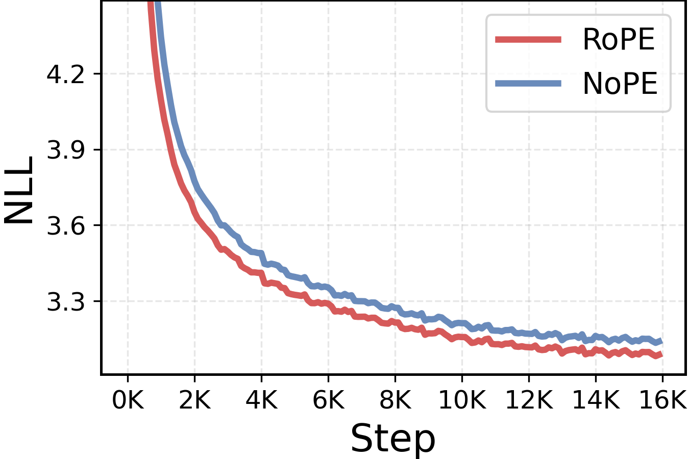
While NoPE transformers were shown to be expressive enough for effective sequence modeling ([25, 21]), we find that they consistently underperform RoPE architectures throughout our experiments. As illustrated in Figure 3, NoPE transformers maintain visibly worse perplexity throughout training. These empirical results are consistent with past literature ([25, 22]), yet the reasons why positional embeddings are key for effective language model training have never been fully understood.

From a purely mechanistic perspective, even without explicit positional embeddings, NoPE transformers can exploit the causal mask to encode positional information, maintaining the same expressivity as their RoPE counterparts ([25, 21]). Specifically, [21] prove that the first attention layer in a NoPE transformer can perfectly reconstruct sequence positions, and subsequent layers can emulate the effects of relative or absolute positional embeddings. As detailed in Section 3.1, rather than looking at theoretical expressivity, we investigate this empirical performance discrepancy from an optimization perspective, providing theoretical analysis of the positional bias of NoPE transformers during training. The theoretical and empirical analysis in this section can be summarized in the following observation.

Observation 1

Positional information and attention non-uniformity, which are crucial for sequence modeling, develop at a bounded rate in NoPE transformers. In contrast, explicit PE methods, such as RoPE, provide a strong bias from the outset and facilitate the propagation of positional information, resulting in faster training. At a high level, our analysis focuses on the rate at which NoPE and RoPE transformers can develop positional bias in their self-attention heads, which captures their non-uniformity. We quantify attention positional bias as a linear functional on the attention map:

Definition 2: Attention positional bias

Given centered positional weights

cij∈Rc_{ij} \in {\mathbb{R}}

with

∑j≤icij=0\sum_{j \leq i} c_{ij} = 0

, the positional bias of the attention weights

αij\alpha_{ij}

Attention heads with a strong positional bias would maximize the average value of

{{\bm{\mathsfit{A}}}}^c

across input sequences for some weights

c

. For example, a "diagonal" attention head, focusing mass on the current token, is exactly the maximizer of

{{\bm{\mathsfit{A}}}}^c

, with

c_{ij}

having

1

s on the diagonal and

−1i−1-\tfrac{1}{i-1}

otherwise.

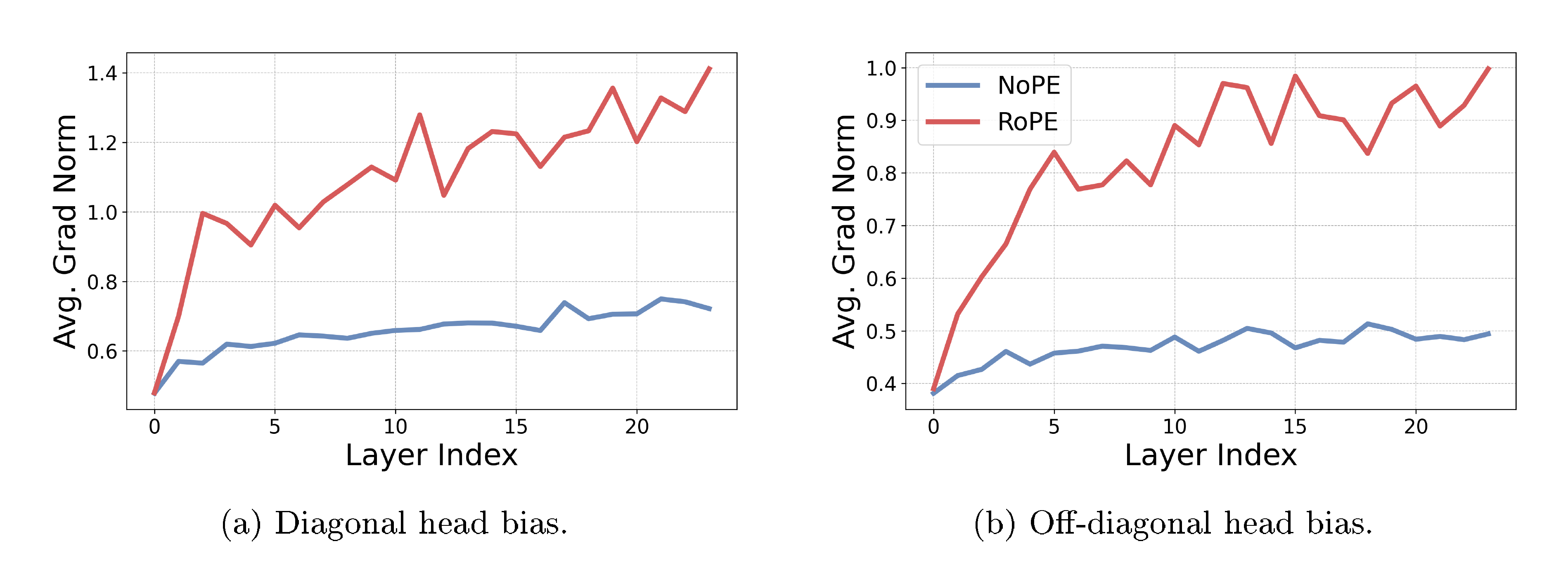
To validate the theory behind Observation 1, we empirically compare the gradients of the attention positional bias functional in attention heads of RoPE and NoPE transformers. Specifically, we measure the average gradient norm at initialization in the direction of two common language modeling patterns: diagonal attention heads, placing mass on the current token, and off-diagonal heads, capturing immediate previous token context. As illustrated in Figure 4, the gradient magnitudes of NoPE transformers are far lower than those of RoPE transformers, with the gap between the two growing in deeper layers. This means that diagonal and off-diagonal heads are slower to develop under NoPE, reflecting its difficulty in recovering positional information. In the next section, we theoretically analyze the causes of this gradient norm gap.

💭 Click to ask about this figure

3.1 Theoretical analysis

We detail our findings, summarized in Observation 1, with a series of formal results, bounding the rate at which positional bias can develop early in training. We provide full proofs and an extended analysis of these results in Appendix B. Throughout this section, we study the sensitivity of the attention positional bias

{{\bm{\mathsfit{A}}}}^c

to the transformer's parameters and interpret

∥∇θAc∥\left\lVert \nabla_{\theta} {{\bm{\mathsfit{A}}}}^c \right\rVert

as bounding the rate at which non-uniform attention patterns can emerge during training.

Warm-up: NoPE transformers break on constant sequences. Before moving to the main theoretical result, we consider a motivating example that illustrates NoPE transformers' training difficulties. Because attention forms a convex combination of value vectors, an attention head applied to a sequence of identical tokens

x1=⋯=xTx_1 = \cdots = x_T

produces identical outputs at every position. Moreover, since normalization layers, MLP blocks, and residual connections act pointwise on tokens, this uniformity propagates through the network. In a NoPE transformer, this means the attention logits are constant over all

\leq i

, hence the post-softmax attention probabilities are uniform. Consequently, the model cannot induce any positional preference and

{{\bm{\mathsfit{A}}}}^c \equiv 0

for any positional weights

c

Proposition 3

Let

M\mathsf{M}

be a NoPE transformer. If the input sequence

(x_1, \dots, x_T)

is comprised of identical tokens

x1=⋯=xTx_1 = \cdots = x_T

, then (1) all attention heads are uniform:

αij=1i\alpha_{ij} = \frac{1}{i}

, (2) query and key gradients vanish:

∂L/∂WQ=∂L/∂WK=0\partial {\mathcal{L}} / \partial W_Q = \partial {\mathcal{L}} / \partial W_K = 0

, (3) for all heads and any positional weights

{{\bm{\mathsfit{A}}}}^c = 0

∇θAc=0\nabla_{\theta} {{\bm{\mathsfit{A}}}}^c = \mathbf{0}

, and (4) the output is constant:

M(x)1=⋯=M(x)T\mathsf{M}(x)_1 = \cdots = \mathsf{M}(x)_T

The explicit positional information injected into attention heads in RoPE transformers circumvents this issue. Enabling non-zero

{{\bm{\mathsfit{A}}}}^c

gradients even on constant sequences.

Proposition 4

For a non-trivial RoPE attention head, even if the input sequence is constant, there are positional weights

c

, for which

{{\bm{\mathsfit{A}}}}^c > 0

, and

∥∇θAc∥>0\left\lVert \nabla_{\theta} {{\bm{\mathsfit{A}}}}^c \right\rVert > 0

NoPE transformers propagate embedding uniformity. At initialization, the entries of the embedding matrix are drawn i.i.d. from a distribution with a fixed small variance (commonly,

σ2=0.02\sigma^2 = 0.02

). Therefore, the token embeddings are close to uniform at the beginning of training. The next theorem shows that for NoPE transformers, this uniformity persists throughout the network, and bounds the attention positional bias

{{\bm{\mathsfit{A}}}}^c

and its gradients.

Theorem 5

Define the he prefix-spread of the hidden states at layer

l

For NoPE transformers, there exists

ε>0\varepsilon > 0

and constants

C_1

C_2

, and

C_3

such that if the initial embeddings

Δh(1)≤ε\Delta_h^{(1)} \leq \varepsilon

, then for all layers

\leq L

with high probability over the initialization distribution. The constants only depend on the number of layers and heads, and not on the sequence length. The main idea in the proof of Theorem 5 is that uniformity in the embeddings causes uniformity in the attention maps, so

αij≈1/i\alpha_{ij} \approx 1 /i

. Uniform mixing of tokens cannot increase the prefix spread; thus, uniformity persists throughout the network. This result explains the discrepancy between RoPE and NoPE transformers illustrated in Figure 4.

In summary, we demonstrate that while NoPE attention can learn positional bias, attention non-uniformity develops slowly early in training due to bounded

{{\bm{\mathsfit{A}}}}^c

gradients at initialization.

4. RoPE prevents effective zero-shot context extension

Show me a brief summary.

In this section, the authors demonstrate that state-of-the-art RoPE scaling methods fail to achieve effective zero-shot generalization to longer contexts because they fundamentally alter attention patterns in ways that harm performance on downstream tasks. While methods like YaRN successfully maintain perplexity on extended sequences, they fail to retrieve information from distant positions, behaving similarly to simply cropping the input to the original training length. This failure stems from an unavoidable trade-off: to keep low-frequency RoPE phases within their training distribution when extending context length, scaling methods must compress these frequencies by approximately the inverse of the extension factor. Since low frequencies dominate semantic attention heads that match content across long distances, this compression warps the learned attention patterns precisely where long-range information retrieval is needed. The analysis reveals that any post-hoc frequency scaling approach must compress low frequencies to avoid out-of-distribution phases, making this limitation inherent to RoPE-based context extension strategies.

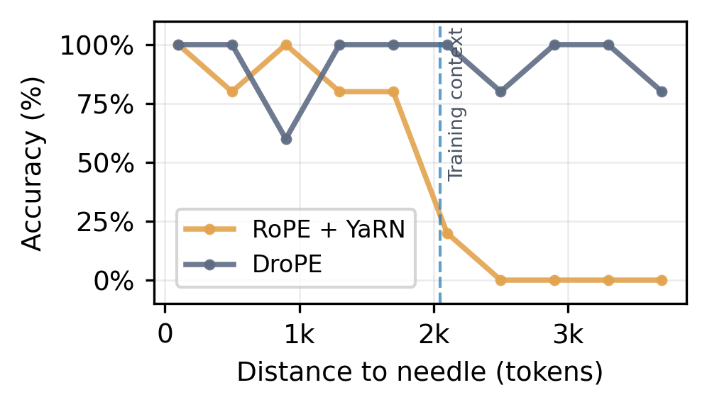
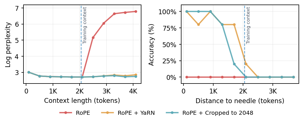
State-of-the-art RoPE scaling methods fail to effectively generalize to sequences longer than those seen in training without additional long-context finetuning. While YaRN and other popular frequency scaling techniques do avoid perplexity degradation on long-context sequence ([13, 14]), they exhibit sharp performance drops on downstream tasks whenever important information is present deep in the sequence, beyond the training context ([24, 26]). We empirically demonstrate this phenomenon, comparing the perplexity and needle-in-a-haystack (NIAH) ([27, 28]) performance of a RoPE transformer scaled with YaRN and to a cropped context baseline. As illustrated in Figure 5, YaRN's zero-shot behavior closely matches that of simply cropping the sequence length to the pretraining context, maintaining constant perplexity but ignoring information present outside the cropped window.

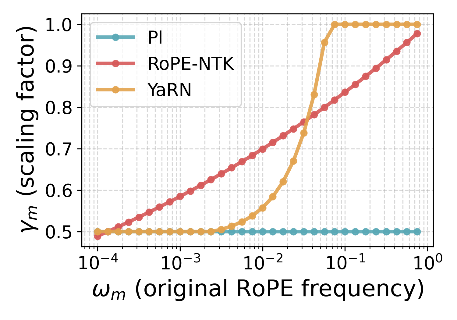
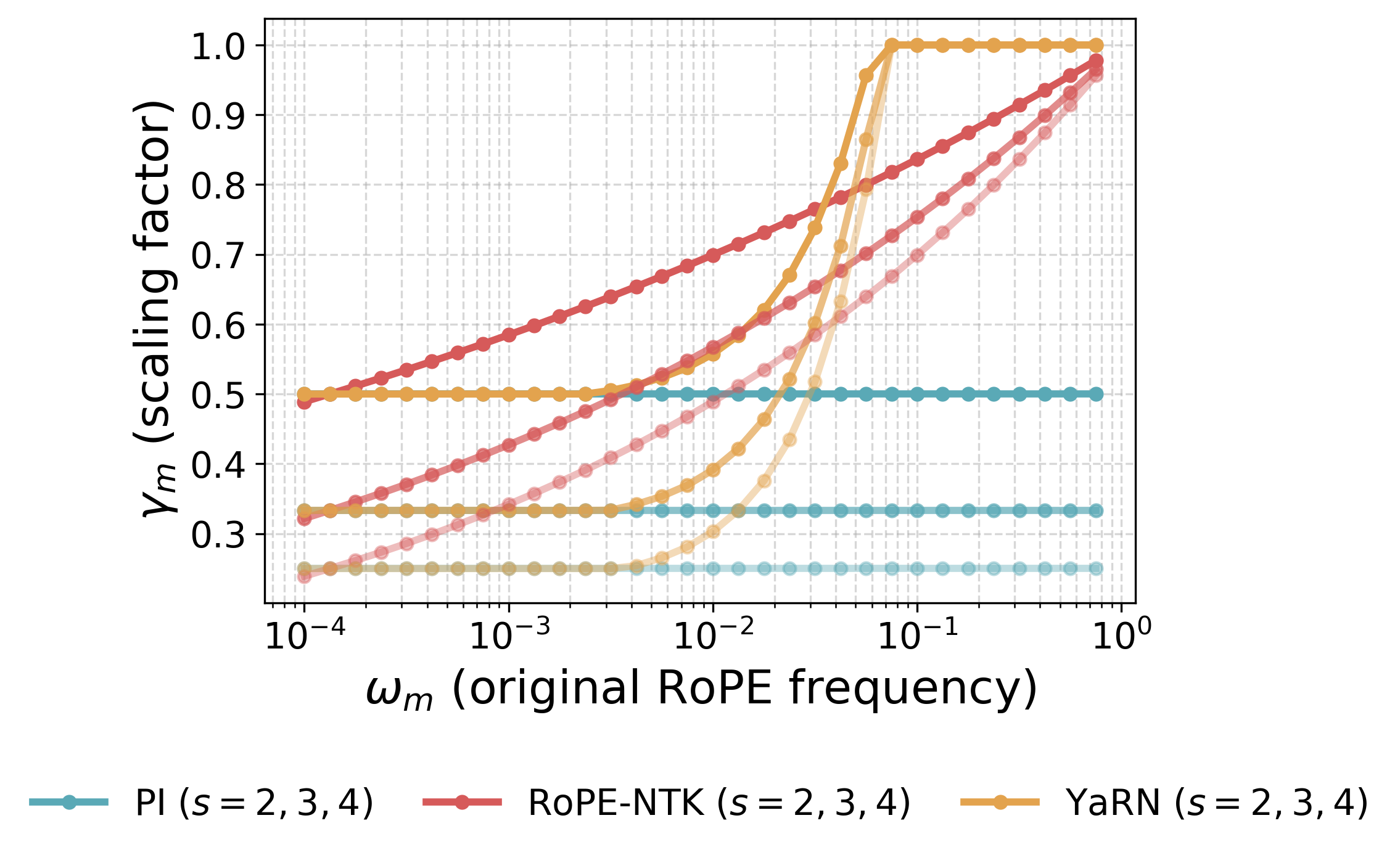
The cause of this limitation lies in the way context extension methods scale different RoPE frequencies. As detailed in Section 2, elaborated on in Appendix A, and illustrated in Figure 6, the scaling factors of PI ([12]), RoPE-NTK ([13]), and YaRN ([14]) have a strong effect on low frequencies. In Section 4.1, we discuss why this aggressive scaling of low frequencies leads to the observed failures, yielding our second observation.

Observation 6

RoPE-scaling methods must compress low frequencies to keep positional phases in-distribution. This, in turn, shifts semantic attention heads at large relative distances, causing the observed failures on downstream tasks, preventing zero-shot context extension.

4.1 Why extrapolation failure is inevitable

Effect of RoPE scaling. RoPE scaling methods modify the frequencies at inference time to evaluate sequences that are longer than those seen during pretraining. In each

2m, 2m{+}1)

subspace, the RoPE phase at relative distance

Δ\Delta

ϕm(Δ)=ωmΔ\phi_m(\Delta)=\omega_m \Delta

, so scaling the frequency to

ωm′=γmωm\omega'_m=\gamma_m \omega_m

is equivalent to using a phase

ϕm′(Δ)=γmωmΔ\phi_m'(\Delta) = \gamma_m \omega_m \Delta

. As illustrated in Figure 6, most scaling methods leave high frequencies nearly unchanged (

γm≈1\gamma_m\approx 1

) but all of them compress the low frequencies (

γm≈1/s\gamma_m \approx 1/s

). As demonstrated both theoretically and empirically in [29], high RoPE frequencies are primarily used by positional heads, with attention patterns based on relative token positions (e.g., diagonal or previous-token heads). In contrast, low frequencies are predominantly used by semantic heads that attend based on query/key content. Consequently, positional heads are largely unaffected by scaling, but semantic attention is shifted. Moreover, the effect on low-frequency dominated semantic heads is exacerbated for distant tokens, since the relative phase

ϕm(Δ)\phi_m(\Delta)

is larger, and thus the

1/ s

scaling factor has a greater effect. In other words, scaling warps low-frequency phases, shifting long-range attention in precisely the subspaces most used for semantic matching.

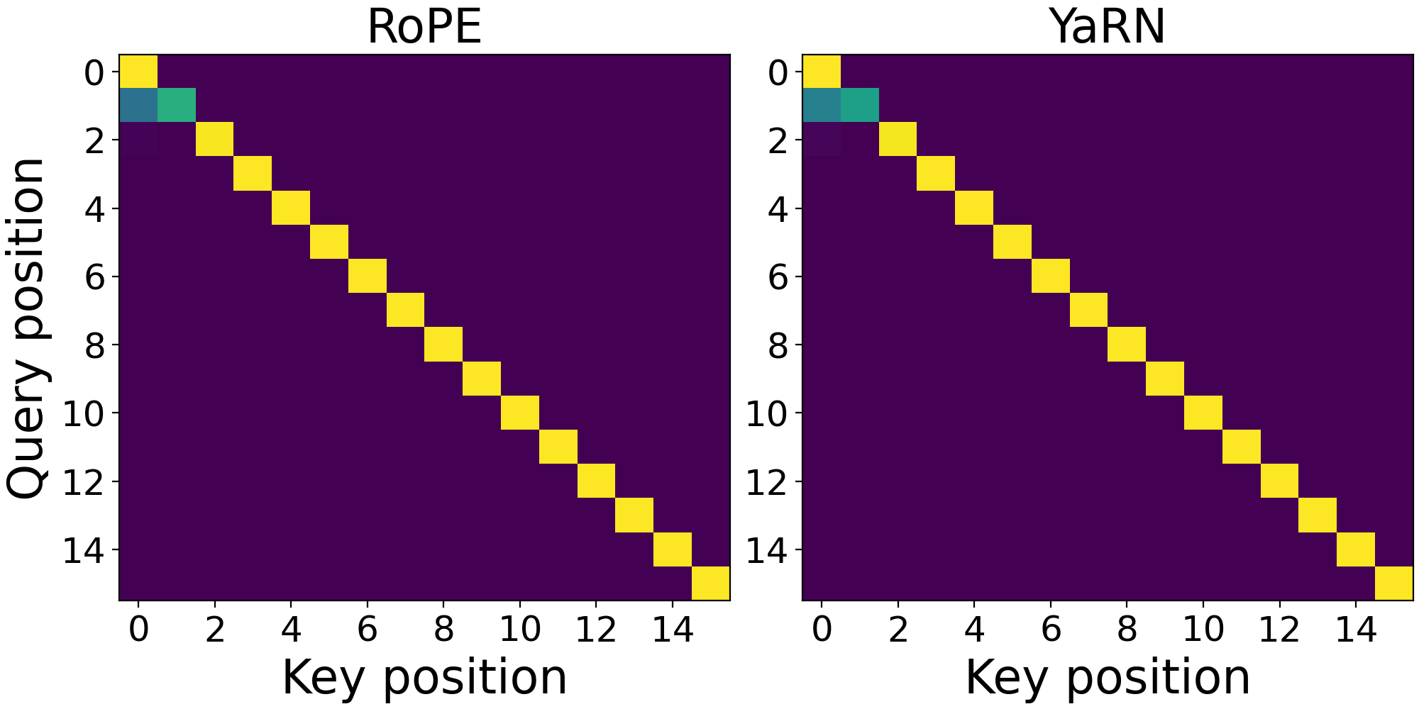
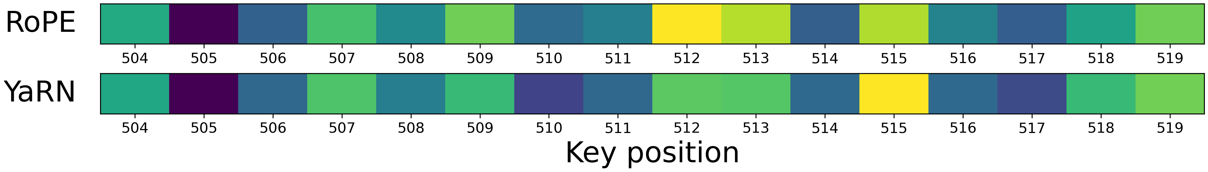
In Figure 7 and Figure 8, we illustrate this behavior in practice. We start by selecting a positional attention head in a pretrained

QWEN2.5-0.5B\text{Q{\scriptsize WEN2.5-0.5B}}

model by examining its average attention positional bias (Definition 2) across layers. In Figure 7, we show the average attention weights in this positional head under YaRN scaling with

s = 2

. Because high frequencies, which are least affected by YaRN, dominate positional heads, the average attention profiles are similar. In Figure 8, we then contrast this behavior with that of a semantic head for a long needle-in-a-haystack sequence, plotting the average attention of the last token (query) with tokens around the needle (keys). YaRN's aggressive scaling of low frequencies substantially shifts attention mass across tokens, reflecting the impact of frequency compression at longer ranges.

Why this is inevitable. In a standard RoPE setup, low-frequency phases never make a full cycle over the original context length:

ϕm(Ctrain)=ωmCtrain<2π\phi_m(C_{\mathrm{train}})=\omega_m C_{\mathrm{train}} < 2 \pi

for small

ωm\omega_m

. E.g. for a standard RoPE base

b = 10^4

, a transformer with head dimension

d_k = 64

, will have at least five low frequencies for which

ϕm(Ctrain)<2π\phi_m(C_\mathrm{train}) < 2 \pi

, even at a training context of

Ctrain=32,000C_\mathrm{train} = 32{, }000

. If we leave

ωm\omega_m

unchanged at an extended length

Ctest>CtrainC_{\mathrm{test}} > C_{\mathrm{train}}

, the new maximal relative phase

ϕm(Ctest)\phi_m(C_{\mathrm{test}})

is pushed outside the training regime and becomes out of distribution for the head. Therefore, to constrain phases to remain in range, any scaling method must choose

γm≤CtrainCtest=1s\gamma_m \le \tfrac{C_{\mathrm{train}}}{C_{\mathrm{test}}} = \tfrac{1}{s}

, which becomes increasingly small as the extension factor

s

grows. In other words, when applying a RoPE transformer to sequences longer than those seen in training, any post-hoc scaling method must compress the low frequencies. But this compression, in turn, shifts attention weights at long relative distances.

5. DroPE: Dropping positional embeddings after pretraining

Show me a brief summary.

In this section, the authors introduce DroPE, a method that removes positional embeddings from pretrained transformers after an initial training phase, enabling strong zero-shot generalization to unseen sequence lengths. The approach leverages the observation that positional embeddings provide crucial inductive bias during training but constrain long-context generalization at inference. DroPE can be integrated at no extra cost by dropping RoPE in the final stages of pretraining, or applied to existing pretrained models through brief recalibration on a fraction of original training tokens. Extensive experiments across model scales from 360M to 7B parameters demonstrate that DroPE recovers over 95% of base model performance after minimal recalibration while substantially outperforming state-of-the-art RoPE scaling methods like YaRN and RoPE-NTK on long-context tasks, achieving improvements of over 10x on LongBench evaluations and enabling effective retrieval at context lengths far beyond those seen during training.

Taken together, Observations Observation 1 and Observation 6 imply that providing explicit positional information with PE is a key component for effective LM training, but is also a fundamental barrier to long-context generalization. This raises a natural question: is it possible to harness the inductive bias from positional embeddings exclusively during training? We answer in the affirmative. In this section, we demonstrate that it is possible to drop all positional embeddings from a pretrained transformer and quickly recover the model's in-context capabilities with a brief recalibration phase. Most notably, this simple new procedure (termed DroPE) unlocks strong zero-shot long context generalization to unseen sequence lengths, far beyond highly-tuned RoPE extensions and prior alternative architectures.

Observation 7

Positional embeddings can be removed after pretraining, allowing LMs to generalize zero-shot to unseen sequence lengths without compromising their in-context performance after short recalibration on a fraction of the training tokens at the original context size.

5.1 Large-scale empirical evaluation

We extensively validate DroPE across different LM and dataset scales, showing it outperforms prior approaches both as a zero cost integration into pretraining recipes and as an inexpensive way to adapt any LM in the wild already pretrained on trillions of tokens. For all experiments in this paper, we provide full implementation details of each evaluated architecture and optimization phase, including comprehensive hyperparameter lists in Appendix C.

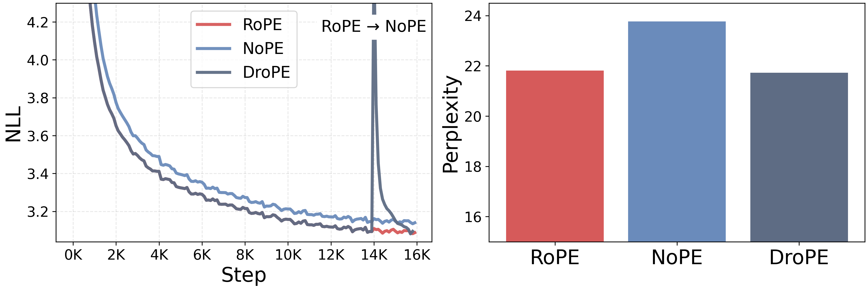
Integrating DroPE at no extra cost. For our first set of experiments, we train from scratch different LMs with half a billion parameters on 16B fineweb tokens ([30]), over twice the chinchilla-optimal rate ([31]). We repeat this recipe for RoPE and NoPE transformers, as well as an ALiBi model ([9]) and an RNoPE-SWA model [22], which are alternative architectures specifically aimed at long-context capabilities. We implement DroPE by taking the 14B tokens RoPE transformer checkpoint, removing positional embeddings from every layer, and resuming training for the final 2B tokens. Despite only recalibrating at the very end of training, at no extra cost, DroPE matches the final in-context validation perplexity of RoPE trained on the full 16B tokens, showing a clear edge over the NoPE baseline trained without positional embedding all the way (Figure 2). We provide further analysis and ablations on the recalibration starting point in Appendix D.1, validating the importance of harnessing the inductive bias of RoPE for a substantial amount of training, in line with the core motivation of our new method.

Table 1: Zero-shot NIAH at $2\times$ training context. Results are reported as a success rate over 500 trials.

Method	Multi- Query	Multi- Key	Multi- Value
RoPE transformer	$0.0$	$0.0$	$0.0$
RoPE transformer + PI	$0.0$	$0.0$	$0.0$
RoPE transformer + RoPE-NTK	$21.1$	$19.4$	$16.5$
RoPE transformer + YaRN	$17.8$	$0.5$	$14.6$

To evaluate the long-context generalization of each method, we select three tasks from the RULER benchmark ([28]): (1) multi-query: retrieve needles for several listed keys, (2) multi-key: retrieve the needle for one specified key, and (3) multi-value: retrieve all needles for one key with a single query. For the base RoPE transformer, we consider three context extension strategies: PI ([12]), NTK-RoPE ([13]), and the popular YaRN ([14]) described in Section 2 and Appendix A. In Table 1, we report the success rate on each task at

2×2\times

the training context length. Our DroPE model substantially outperforms all baselines in each setting. While RoPE-NTK and YaRN also yield improvements to the original RoPE transformer, they consistently trail DroPE, as most evident on the multi-key task. In contrast, specialized architectures such as ALiBi, RNoPE-SWA, and NoPE underperform on multi-query tasks, which are the logic-intensive setting where strong base models excel. We believe these results provide compelling evidence toward validating DroPE's potential to be integrated as a standard component in the training pipeline of future generations of LMs.

Extending the context of LMs in the wild with DroPE. For our second set of experiments, we directly apply DroPE to a 360M parameter language model from the

SMOLLM\text{S{\scriptsize MOL}L{\scriptsize M}}

family ([32]) family pretrained on 600 billion tokens. We perform DroPE's recalibration with continued pretraining using the same context length, data, and hyperparameters as reported by [32]. We consider three different recalibration budgets of 30, 60, and 120 billion tokens, adjusting the learning rate schedule accordingly. Given the extended training periods, only for these experiments, we also add QKNorm ([33]) after dropping the positional embeddings, which we find beneficial for mitigating training instabilities, as noted by [34] (See Appendix D.3).

Table 2: DroPE outperforms RoPE-scaling methods on long context-tasks. We evaluate $\text{S{\scriptsize MOL}L{\scriptsize M-} D{\scriptsize RO}P{\scriptsize E}}$ and the base $\text{S{\scriptsize MOL}L{\scriptsize M}}$ model, extended with different RoPE scaling methods, on four long context language modeling tasks from [35] and needle-in-a-haystack.

Method	MultiFieldQA	MuSiQue	GovReport	LCC	NIAH	Avg.
SmolLM	$4.03$	$0.4$	$4.48$	$5.99$	$0.0$	$2.98$
SmolLM + PI	$13.68$	$2.45$	$5.67$	$11.52$	$0.0$	$6.66$
SmolLM + RoPE-NTK	$18.87$	$4.89$	$\mathbf{23.71}$	$8.26$	$29.84$	$17.11$
SmolLM + YaRN	$20.78$	$4.77$	$15.03$	$10.87$	$48.25$	$19.94$
SmolLM- DroPE	$\mathbf{29.33}$	$\mathbf{7.93}$	$21.87$	$\mathbf{18.56}$	$\mathbf{74.92}$	$\mathbf{30.52}$

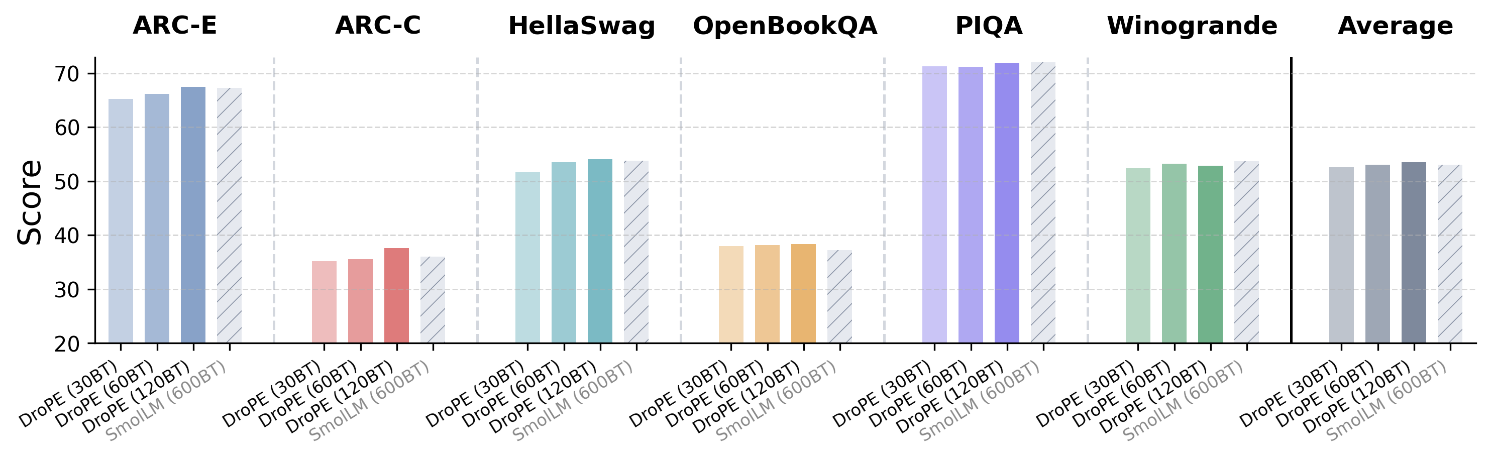
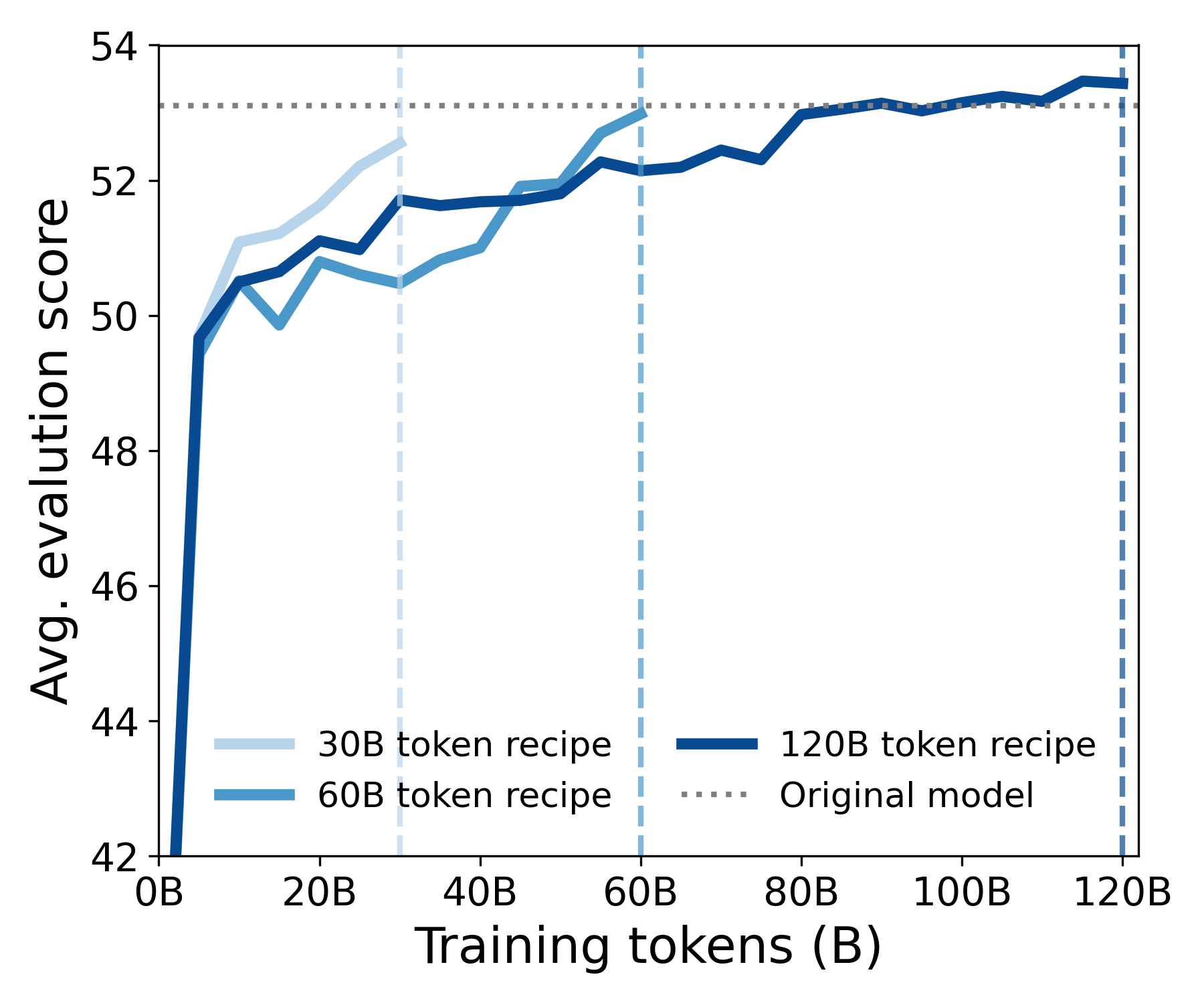
We start by analyzing how quickly our

DROPE\text{S{\scriptsize MOL}L{\scriptsize M-} D{\scriptsize RO}P{\scriptsize E}}

models can recover

SMOLLM\text{S{\scriptsize MOL}L{\scriptsize M}}

's in-context performance across six different LM reasoning benchmarks ([36, 37, 38, 39, 40]). As shown in Figure 9 and Figure 10 as well as Table 5, even with our shortest training schedule,

DROPE\text{S{\scriptsize MOL}L{\scriptsize M-} D{\scriptsize RO}P{\scriptsize E}}

almost entirely matches

SMOLLM\text{S{\scriptsize MOL}L{\scriptsize M}}

on every task, while with our longest schedule our new model manages to exceed its original performance. Furthermore, inspecting our model at every checkpoint throughout training, we find that DroPE recovers over 95% of $SMOLLM\text{S{\scriptsize MOL}L{\scriptsize M}}$ 's performance after less than 5B tokens, representing a minuscule

0.8%0.8\%

SMOLLM\text{S{\scriptsize MOL}L{\scriptsize M}}

's original budget.

We then evaluate our

DROPE\text{S{\scriptsize MOL}L{\scriptsize M-} D{\scriptsize RO}P{\scriptsize E}}

models' zero-shot length generalization on four different tasks from LongBench ([35]), a challenging benchmark even for closed-source LMs, including knowledge-extraction problems longer than 80 times

SMOLLM\text{S{\scriptsize MOL}L{\scriptsize M}}

's pretraining context (

2048

tokens). We compare our method with the base

SMOLLM\text{S{\scriptsize MOL}L{\scriptsize M}}

and three RoPE extensions: PI, RoPE-NTK, and YaRN. As shown in Table 2, despite a significant difficulty spike compared to our prior evaluations, DroPE still displays a clear edge over prior approaches, improving the base

SMOLLM\text{S{\scriptsize MOL}L{\scriptsize M}}

's average score by over 10 times. These gains are far beyond all prior zero-shot RoPE extensions currently used across modern LMs. We refer to Appendix D.2 for a fine-grained analysis of task performance as a function of extension factor.

Scaling to billion-parameter models. Given the remarkable efficiency of recalibration, we test DroPE's ability to scale to larger LMs in the wild, such as

SMOLLM-1.7B\text{S{\scriptsize MOL}L{\scriptsize M-1.7B}}

([32]) and

LLAMA2-7B\text{L{\scriptsize LAMA2-7B}}

([41]), which were trained on 1 trillion and 4 trillion tokens, respectively. For both of these models, we perform recalibration on 20B tokens, which only represents 2% of the pretraining budget for

SMOLLM-1.7B\text{S{\scriptsize MOL}L{\scriptsize M-1.7B}}

, and only

0.5%0.5\%

for

LLAMA2-7B\text{L{\scriptsize LAMA2-7B}}

. As demonstrated in Table 3, consistently with all our prior results on a smaller scale,

DROPE\text{S{\scriptsize MOL}L{\scriptsize M-1.7B-} D{\scriptsize RO}P{\scriptsize E}}

and

DROPE\text{L{\scriptsize LAMA2-7B-} D{\scriptsize RO}P{\scriptsize E}}

once again outperform state-of-the-art RoPE-scaling methods on long-context question-answering and summarization, providing strong evidence towards the scalability and immediate potential of DroPE.

Table 3: Length generalization results on larger models. We evaluate DroPE on $\text{S{\scriptsize MOL}L{\scriptsize M-1.7B}}$ and $\text{L{\scriptsize LAMA2-7B}}$ , and compare it against different RoPE scaling methods, on long context language modeling tasks from [35]. We don't include the LCC task since it is in context for $\text{L{\scriptsize LAMA2-7B}}$ .

Model	Method	MultiFieldQA	MuSiQue	GovReport	Avg.
SmolLM-1.7B	Base	4.12	0.50	4.70	3.11
	RoPE-NTK	27.58	3.37	24.65	18.53
	YaRN	27.60	3.90	17.19	16.23
	DroPE	32.18	7.53	24.77	21.49

Overall, our in-context and out-of-context results demonstrate DroPE is an efficient and effective long-context extension method, which we believe can have meaningful implications for reducing the cost of training pipelines and for tackling the canonical context scalability challenges of transformers. We complement this section with additional experimental results, including the entire LongBench benchmark, and a performance by query length breakdown in Appendix D.

6. Related work

Show me a brief summary.

In this section, the authors position DroPE within the landscape of existing positional embedding methods for transformers. Recent RoPE improvements include variants using Fourier and wavelet transforms, as well as methods like p-RoPE, NRoPE-SWA, and SWAN-GPT that blend characteristics of RoPE and NoPE architectures. DroPE represents a fundamentally different paradigm by replacing RoPE with NoPE at different training stages rather than modifying the positional embedding scheme itself. These alternative RoPE variants are complementary to DroPE and could potentially substitute for RoPE within the DroPE training framework. Another research direction maintains dedicated positional vectors while modifying their indexing or adaptivity to achieve length generalization. The key distinction is that DroPE treats positional embeddings as a temporary training scaffold to be removed, whereas other methods focus on designing better positional embedding schemes that remain throughout the model's lifetime.

Recent improvements to RoPE include variants based on Fourier and wavelet transforms ([42, 43]) and methods such as

p

-RoPE ([44]), NRoPE-SWA ([22]), and SWAN-GPT ([23]), which occupy a middle ground between RoPE and NoPE. Our approach represents a fundamentally different paradigm, replacing RoPE with NoPE at different stages of training. These directions are complementary to ours and can be used in place of RoPE within the DroPE framework. Another orthogonal direction seeks length generalization while retaining a dedicated positional vector yet modifying its indexing or adaptivity ([45, 46, 47]).

7. Discussion and extensions

Show me a brief summary.

In this section, the authors reinterpret positional embeddings in transformer language models as a training-time inductive bias that enables efficient learning but fundamentally limits zero-shot generalization to longer contexts than seen during training. This tension motivates DroPE, a method that treats positional embeddings as temporary scaffolding to be removed after pretraining, followed by brief recalibration without them. Empirical validation across multiple model sizes and datasets demonstrates that DroPE not only matches in-context performance of the original models but also significantly outperforms existing context extension techniques in zero-shot long-context tasks. The approach reveals that architectural trade-offs traditionally viewed as fixed can be reconciled by strategically varying architectural components across training and inference stages. This work establishes DroPE as a viable component for future training pipelines and suggests a broader paradigm shift toward stage-specific architectural choices to overcome fundamental limitations in AI systems.

Our findings support a reinterpretation of positional embeddings in transformer LMs as a useful inductive bias that is essential for efficient training (Observation 1), but inherently constrains zero-shot context extension (Observation 6). Based on these findings, we propose DroPE, a new method rethinking the conventional role of PEs as a temporary scaffold that can and should be removed after serving their training-time purpose (Observation 7). We empirically validate DroPE across different models and data scales, showing its effectiveness and potential to be integrated as a new core component of future state-of-the-art training pipelines. More broadly, our work demonstrates that canonical trade-offs in LM architecture design can be reconciled by employing different architectural choices for different stages of the training and inference pipelines and recalibrating the model for the new architecture. We hope this will inspire further research toward challenging established bottlenecks in AI.

Acknowledgments

Show me a brief summary.

In this section, the authors acknowledge the funding support that enabled this research work. Specifically, researcher YG received financial support from the United Kingdom Research and Innovation Engineering and Physical Sciences Research Council through their Centre for Doctoral Training in Autonomous and Intelligent Machines and Systems, under grant reference EP/S024050/1. This brief acknowledgment serves to recognize the institutional backing that made the DroPE research possible, highlighting the role of UK-based research councils in advancing fundamental work on transformer language models and their positional embedding architectures. The acknowledgment reflects standard academic practice of crediting funding bodies that support doctoral training programs and associated research activities in artificial intelligence and machine learning.

YG is supported by the UKRI Engineering and Physical Sciences Research Council (EPSRC) CDT in Autonomous and Intelligent Machines and Systems (grant reference EP/S024050/1).

Author contribution

Show me a brief summary.

In this section, the authors delineate the collaborative contributions behind the DroPE methodology. Yoav Gelberg spearheaded the project, driving the empirical and theoretical analysis while contributing substantially to codebase development, method design, training pipelines, experimentation, and manuscript preparation. Koshi Eguchi supported experimental work and provided critical infrastructure for scaling the approach to larger models and datasets. Takuya Akiba served as project advisor, participating in foundational discussions about method design and contributing to the written presentation. Edoardo Cetin co-led development efforts, making major contributions to codebase implementation, method design, experimentation, and writing, while specifically leading the engineering of DroPE's training pipeline and coordinating overall project execution. The collaborative structure reflects a division of labor spanning theoretical foundations, empirical validation, infrastructure development, and technical implementation necessary to establish DroPE as a practical solution for extending language model context lengths.

Yoav Gelberg led the project, made major contributions to the codebase, method design, training pipelines, experimentation, and writing. He led DroPE's empirical and theoretical analysis.

Koshi Eguchi made contributions to experimentation and provided infrastructure support for scaling the methodology.

Takuya Akiba advised the project, was involved in early discussions about method design, and contributed to writing.

Edoardo Cetin made major contributions to the codebase, method design, experimentation, and writing. He led engineering on DroPE's training pipeline and coordinated the project.

Appendix

A. Extended preliminaries

Attention.

Throughout this section, we consider a pre-norm, decoder-only transformer with

L

layers,

H

attention heads per layer, model dimension

d_\mathrm{model}

, and head dimension

d_k

h1(l),…,hT(l)∈Rdh^{(l)}_1, \dots, h^{(l)}_T\in {\mathbb{R}}^{d}

denote the representations fed into the

l

-th multi-head attention block. For a head

h

in layer

l

, queries, keys, and values are computed by

The attention scores and weights are then computed by

s_{ij}^{(l, h)}

are referred to as attention logits or scores and

αij(l,h)\alpha_{ij}^{(l, h)}

are referred to as attention weights or probabilities. Note that the softmax is taken over

\leq i

, implementing a causal mask. The output of the multi-head attention block is

where

[⋅,…,⋅][\cdot, \dots, \cdot]

represents concatenation along the feature dimension. When clear from context, we omit layer and head indices.

Positional embeddings in transformers.

The attention mechanism does not directly encode relative distances between queries and keys. Therefore, attention is invariant to prefix permutations: for any permutation

σ∈Sp\sigma \in S_p

of the first

p

input tokens,

attn(xσ−1(1),…,xσ−1(p),xp,…,xT)i=attn(x1,…,xT)i\mathrm{attn}(x_{\sigma^{-1}(1)}, \dots, x_{\sigma^{-1}(p)}, x_p, \dots, x_T)_i = \mathrm{attn}(x_1, \dots, x_T)_i

for every

i > p

. In other words, pure attention is blind to token positions. To address this, [5] introduced absolute positional embeddings, adding position information to the token embeddings before the first transformer block. More recently, many architectures replace absolute embeddings with relative schemes that inject pairwise positional information directly into the attention mechanism. The most widely used approach is Rotary Position Embedding (RoPE) ([11]). RoPE modifies the attention scores in Equation 4 by rotating queries and keys before taking their inner product:

where,

\in O(d_k)

is a block-diagonal orthogonal matrix composed out of

\times 2

rotation blocks:

In the standard RoPE parameterization,

ωm=b−2m−1dk\omega_m = b^{-2\frac{m-1}{d_k}}

with

b = 10{, }000

Language model context extension.

Generalizing to contexts longer than those seen during training is a key challenge for transformer-based language models. The key issue is that when applying a transformer on a longer context, the attention mechanism must operate over more tokens than it was trained to handle. This issue is exacerbated with RoPE: applying RoPE to sequences beyond the training length introduces larger position deltas, and thus larger rotations, pushing attention logits out of the training distribution. RoPE context-extension methods address this by rescaling the RoPE frequencies when the inference context length exceeds the training context length. Let

CtrainC_\mathrm{train}

be the training context and

Ctest>CtrainC_\mathrm{test}>C_\mathrm{train}

the target context with extension factor

C_\mathrm{test} / C_\mathrm{train}

. Such methods define new frequencies

using scaling factors

γm=γm(s)\gamma_m = \gamma_m(s)

. E.g. Position Interpolation (PI) ([12]), uses a uniform scaling of

NTK-RoPE ([13]) uses

so that low frequencies (

\approx d_k/2

) are scaled similarly to PI and for high frequencies

γm≈1\gamma_m \approx 1

. YaRN ([14]) uses

with tunable

p

and

q

parameters, originally chosen as

p = 1

q = 32

. See Figure 11 for a comparison between these different RoPE scaling methods with

s = 2

3

, and

4

B. Theoretical results and proofs

In this section, we analyze the behavior of positional bias, or attention non-uniformity, in NoPE transformers and RoPE transformers early in training. We provide formal statements and proofs for all the results from Section 3, starting with Proposition 3 and Proposition 4, followed by Theorem 5. The notation of this section follows that of Appendix A.

B.1 Proof of Proposition 3

Proof: Let

x1,…,xTx_1, \dots, x_T

be a constant input sequence,

x1=⋯=xTx_1 = \cdots = x_T

, and let

M\mathsf{M}

be a NoPE transformer, i.e. a transformer with no positional encodings and causal self attention. The order of the proof is (4)

⇒\Rightarrow

(1)

⇒\Rightarrow

(2 + 3).

(4) Layer outputs, and thus model outputs, are constant. At the first layer, inputs are identical

h1(1)=⋯=hL(1)=hh_1^{(1)} = \cdots = h_L^{(1)} = h

. This means that for every attention head and every

\leq j \leq T

Therefore, the output of the attention head is

independent of

i

. Concatenating heads and applying

W_O

preserves equality across positions. Residual connections, LayerNorm, and the MLP are positionwise (the same function is applied independently at each position), so identical inputs produce identical outputs at every position. Thus the layer output remains constant. By repeating this argument layer-by-layer, every subsequent layer receives identical inputs and outputs identical states, so in the end

(1) Uniform causal attention. Using (4), we know that for every layer

\leq l \leq L

Therefore, for every attention head and every

\leq j \leq T

Thus, for each

\leq j \leq i \leq T

, the attention scores

sij=q⊤k/dk≡cs_{ij} = q^\top k/\sqrt{d_k} \equiv c

are constant (independent of

i

j

). Hence

(2 + 3) Vanishing $W_Q, W_K$ gradients. Since, the inputs for every layer are constant, we know from (1) that every attention head has

αij≡1/i\alpha_{ij} \equiv 1/i

, independant of $W_Q$ and $W_K$ . Therefore

∂αij/∂WQ=∂αij/∂WK=0\partial \alpha_{ij} / \partial W_Q = \partial \alpha_{ij} / \partial W_K = 0

. Since the attention bias

{{\bm{\mathsfit{A}}}}^c

depends on the parameters

{\theta}

only through

αij\alpha_{ij}

and the loss

{\mathcal{L}}

depends on

W_Q

and

W_K

only through

αij\alpha_{ij}

, all these gradients vanish. More formally, using the chain rule,

\begin{gather*} \frac{\partial {{\bm{\mathsfit{A}}}}^c}{\partial {\theta}} = \frac{1}{T}\sum_{1 \leq j \leq i \leq T} c_{ij} \frac{\partial \alpha_{ij}}{\partial {\theta}} = 0, \\ \frac{\partial {\mathcal{L}}}{\partial W_Q} = \sum_{1 \leq j \leq i \leq T} \frac{\partial {\mathcal{L}}}{\partial \alpha_{ij}} \frac{\partial \alpha_{ij}}{\partial W_Q} = 0, \qquad \frac{\partial {\mathcal{L}}}{\partial W_K} = \sum_{1 \leq j \leq i \leq T} \frac{\partial {\mathcal{L}}}{\partial \alpha_{ij}} \frac{\partial \alpha_{ij}}{\partial W_K} = 0. \end{gather*}

💭 Click to ask about this equation

Additionally, since the heads are uniform the attention bias is zero to begin with

Remark.

Note that part (4) of the proposition holds for RoPE transformers as well. Parts (1), (2) and (3) do not. The relative rotations break attention uniformity and thus changing the magnitude of

∥WQ∥\left\lVert W_Q \right\rVert

and

∥WK∥\left\lVert W_K \right\rVert

can affect the attention weights. This is formally demonstrated in the next section.

B.2 Proof of Proposition 4

Proof: Let

x1=⋯=xT=x∈Rdx_1 = \cdots = x_T = x \in {\mathbb{R}}^d

be the inputs to a RoPE attention head, and let

WQ,WK∈Rdk×dW_Q, W_K \in {\mathbb{R}}^{d_k \times d}

be the query and key projection parameters. Since the projection maps are shared across tokens, the queries and keys are constant as well:

Set the positional bias weights to be

Since

∑j≤iαij=1\sum_{j \leq i} \alpha_{ij} = 1

, we have

∑j≤icij=0\sum_{j \leq i} c_{ij} = 0

as required. The positional bias

{{\bm{\mathsfit{A}}}}^c

By Cauchy-Schwarz,

with equality only when

αi1=⋯=αii\alpha_{i1} = \cdots = \alpha_{ii}

. Therefore,

with equality iff

αij=1/i\alpha_{ij} = 1/i

is uniform. Therefore,

{{\bm{\mathsfit{A}}}}^c > 0

unless

αij\alpha_{ij}

is uniform for all

i

. The following lemma asserts that this is not the case

Lemma 8

For any non-degenerate RoPE head and input embeddings

x1=⋯=xt=xx_1 = \cdots = x_t = x

, there exists

\geq 1

such that

si1,…,siis_{i1}, \dots, s_{ii}

and

αi1,…,αii\alpha_{i1}, \dots, \alpha_{ii}

are not uniform.

The proof of Lemma 8 is at the end of this subsection. As for

∇θAc\nabla_{\theta} {{\bm{\mathsfit{A}}}}^c

, rewrite

{{\bm{\mathsfit{A}}}}^c

so the dependence in the parameters

{\theta}

is entirely through

From the definition of RoPE, we have

Consider scaling

q

by a scalar

λ>0\lambda>0

\mapsto \lambda q

. For fixed prefix

i

, define

Then

F_i(\lambda) = \frac{Z_i(2\lambda)}{Z_i(\lambda)^2} \quad \Longrightarrow \quad \frac{d}{d\lambda} \log F_i(\lambda)=2 \underbrace{\mathbb{E}_{j \sim \alpha_i(2\lambda)}[s_{ij}]}_{A_i'(2\lambda)} -2 \underbrace{\mathbb{E}_{j \sim \alpha_i(\lambda)}[s_{ij}]}_{A_i'(\lambda)},

💭 Click to ask about this equation

where

Ai(λ):=log⁡Zi(λ)A_i(\lambda) := \log Z_i(\lambda)

is the log-partition function. The second derivative of the log partition function is the logit variance

A_i''(\lambda) = \frac{Z_i''(\lambda)Z_i(\lambda) - (Z_i'(\lambda))^2}{(Z_i(\lambda))^2} = \frac{\sum_{j \leq i} s_{ij}^2 e^{\lambda s_{ij}}}{Z_i(\lambda)} - \left(\frac{\sum_{i \leq j} s_{ij} e^{\lambda s_{ij}}}{Z_i(\lambda)}\right)^2 = \mathrm{Var}_{j \sim \alpha_i(\lambda)}(s_{ij})

💭 Click to ask about this equation

therefore

Ai′′(λ)=Varαi(λ)(si⋅)>0A_i''(\lambda)=\mathrm{Var}_{\alpha_i(\lambda)}(s_{i\cdot})>0

since from Lemma 8

s_{ij}

are not all equal and

αij(λ)>0\alpha_{ij}(\lambda) > 0

. Thus,

Ai′(λ)A_i'(\lambda)

is strictly increasing in

λ\lambda

. Hence, for any

i

with non-constant logits,

and in particular at

λ=1\lambda = 1

By the chain rule for

\mapsto \lambda q

Thus

∇qFi(q)≠0\nabla_q F_i(q)\neq 0

(otherwise the dot product with

q

couldn’t be strictly positive). Finally, since

q = W_Qx

and with

x≠0x\neq 0

we get

∥∇θFi∥≥∥∇WQ∥Fi>0\left\lVert \nabla_{\theta} F_i \right\rVert \geq \left\lVert \nabla_{W_Q} \right\rVert F_i > 0

. Therefore

has strictly positive norm (a sum of nonzero matrices sharing the same nonzero right factor

x⊤x^\top

cannot be the zero matrix unless all left factors vanish, which they don’t for

\ge 2

To conclude this section, we now prove Lemma 8.

Proof: RoPE acts as independent

2×22\times 2

rotations on disjoint coordinate pairs. Thus

with pairwise distinct frequencies

ωm∈(0,2π)\omega_m \in(0, 2\pi)

. Decompose

s_{ij} = f(j-i)

where

Let

For any

\in {\mathbb{R}}^2

Define

Am:=qm⊤kmA_m := q_m^\top k_m

and

Bm:=qm⊤JbmB_m := q_m^\top J b_m

. Then

\begin{split} f(\Delta) = \frac{1}{\sqrt{d_k}}\sum_{m=1}^{M}\Big(A_m\cos(\Delta \omega_m) + B_m\sin(\Delta \omega_m)\Big) &= \Re\left(\sum_{m=1}^{M} c_m e^{i\Delta \omega_m}\right) \\ &= \frac{1}{2}\sum_{m = 1}^M C_m e^{i\Delta \omega_m} + \bar{C}_m e^{-i \Delta \omega_m}, \end{split}

💭 Click to ask about this equation

where

Assume

f(Δ)f(\Delta)

is constant in

Δ\Delta

for

Δ=0,…,2M=dk\Delta = 0, \dots, 2M = d_k

, and denote the constant value by

−12C0-\frac{1}{2}C_0

. Then we have

were

C−m:=CˉmC_{-m} := \bar{C}_m

, and

ω−m=−ωm\omega_{-m} = -\omega_m

. Since

{e−iωM,…,e−iω1,1,eiω1,…,eiωM}\{e^{-i \omega_M}, \dots, e^{-i \omega_1}, 1, e^{i \omega_1}, \dots, e^{i \omega_M}\}

are all distinct, by Vandermonde's identity this means

Cm=Cˉm=0C_m = \bar{C}_m = 0

for

\dots, M

⇒Am=Bm=0\Rightarrow A_m = B_m = 0

for

\dots, M

. Now

A_m = B_m = 0

means

km≠0k_m \neq 0

, then

{k_m, J k_m\}

spans

{\mathbb{R}}^2

, forcing

q_m=0

. Thus for every block

m

, either

q_m = 0

k_m = 0

, which results in a degenerate RoPE head, contradicting the assumption. Therefore, for

\geq d_k + 1

the attention logits

s_{ij}

are not constant, and thus the attention weight

αij\alpha_{ij}

are not constant.

B.3 Proof of Theorem 5

In this section, we prove Theorem 5. To do so, we first need to prove a sequence of Propositions and Lemmas. First, we restate the theorem here. Since all weight matrices are drawn from a Gaussian distribution with a fixed variance, there exists a constant

B

, depending only on the architecture, such that with high probability the operator norms of

W_Q

W_K

W_V

, and

W_O

, as well as the Lipschitz constants of the MLPs and normalization layers are all bounded by

B

. To see this use, e.g. Theorem 4.4.5 from [48] and the fact that for a two layer MLP

f

, it's Lipschitz constnat is bounded by

Lip(f)≤∥W1∥∥W2∥Lip(σ)\mathrm{Lip}(f) \leq \left\lVert W_1 \right\rVert \left\lVert W_2 \right\rVert \mathrm{Lip}(\sigma)

. Let

L

be the number of layers, and

H

be the number of attention heads per layer. For any vector sequence

ai∈Rda_i \in {\mathbb{R}}^d

we denote by

aˉi=1i∑j≤iaj\bar{a}_i = \frac{1}{i} \sum_{j \leq i} a_j

the prefix sum of

a_i

. For real sequences with two indices

aij∈Ra_{ij} \in {\mathbb{R}}

we denote

ai=(ai1,…,aii)∈Ria_i = (a_{i1}, \dots, a_{ii}) \in {\mathbb{R}}^i

and

aˉi=1i∑j≤iaij\bar{a}_i = \frac{1}{i}\sum_{j \leq i} a_{ij}

Proposition 9

Fix a row

i

in an attention head at the

l

-th layer.

Proof: Notice that

Therefore, by Cauchy-Swartz

By the linearity of

W_K

we get

∥kj−kˉi∥=∥WK(hj−hˉi)∥≤∥WK∥∥hj−hˉi∥≤∥WK∥Δh(l)≤BΔh(l)\left\lVert k_j-\bar{k}_i \right\rVert=\left\lVert W_K(h_j-\bar{h}_i) \right\rVert \le \left\lVert W_K \right\rVert\left\lVert h_j-\bar{h}_i \right\rVert\leq \left\lVert W_K \right\rVert\Delta_h^{(l)} \leq B \Delta_h^{(l)}

. As for

∥qi∥=∥WQhi∥\left\lVert q_i \right\rVert = \left\lVert W_Q h_i \right\rVert

, recall that

h_i

are the output of a normalization layer, and therefore (at initialization)

∥hi∥=d\left\lVert h_i \right\rVert = \sqrt{d}

. Thus,

∥qi∥≤Bd\left\lVert q_i \right\rVert \leq B \sqrt{d}

. Putting it all together gives

To finish the proof, take a maximum over

\leq i

To bound the effect on the attention probabilities, we need the following Lemma.

Lemma 10

For any

\in {\mathbb{R}}^n

Proof: A

C^2

convex function

{\mathbb{R}}^n \to {\mathbb{R}}

satisfies

∥∇f(x)−∇f(y)∥1≤∥x−y∥∞\left\lVert \nabla f(x)-\nabla f(y) \right\rVert_1 \leq \left\lVert x-y \right\rVert_\infty

(1-smoothness) if

d⊤∇2f(x)d≤∥d∥∞2d^\top \nabla^2 f(x) d \leq \left\lVert d \right\rVert_\infty^2

for all

\in {\mathbb{R}}^n

(see Theorem 2.1.6 in [49]). Take

\log\Big(\sum_{i = 1}^n e^{x_i}\Big)

f

C^2

, convex and

∇f(x)=softmax(x)\nabla f(x) = \mathrm{softmax}(x)

. Therefore, all we need to show is that for all

\in {\mathbb{R}}^n

and indeed,

\begin{split} d^\top \nabla \mathrm{softmax}(x) d &= d^\top\mathrm{diag}(\mathrm{softmax}(x)) d - (\mathrm{softmax}(x)^\top d)^2 \\ &\leq d^\top \mathrm{diag}(\mathrm{softmax}(x))d \\ &\leq \left\lVert d \right\rVert_\infty^2 \left\lVert \mathrm{softmax}(x) \right\rVert_1 \\ &=\left\lVert d \right\rVert_\infty^2, \end{split}

💭 Click to ask about this equation

as required.

Using Lemma 10, we can bound the uniformity of

αij\alpha_{ij}

and the prefix spread of the head outputs.

Proposition 11

Let

ui=1i1∈Riu_i = \frac1i \bm{1} \in {\mathbb{R}}^i

. In any layer

l

and,

Proof: To get Equation 8, let

a

be the constant vector

(sˉi,…,sˉi)∈Ri(\bar{s}_i, \dots, \bar{s}_i) \in {\mathbb{R}}^i

and let

b = s_i - a

. By Lemma 10

Now, notice that

∥b∥∞=max⁡j≤i∣sij−sˉi∣\left\lVert b \right\rVert_\infty = \max_{j \leq i} \big|s_{ij} - \bar{s}_i\big|

, therefore Proposition 9 gives us the desired inequality. For Equation 9 notice that,

hence

We now bound the next layer's spread in terms of the current one. Denote by

Δz(l):=max⁡imax⁡j≤i∥zj−zˉi∥\Delta_z^{(l)}:=\max_{i}\max_{j\le i}\left\lVert z_j-\bar{z}_i \right\rVert

the prefix spread of an attention head's output. First, we'll give a bound for

Δz(l)\Delta_z^{(l)}

, and then use this bound to prove the entire propagation result. Before, we need a short lemma.

Lemma 12

For any sequence

x_j)

and

\leq i

Proof:

xˉj−xˉi=1j∑r≤j(xr−xˉi)\bar{x}_j-\bar{x}_i= \frac1j \sum_{r\le j}(x_r-\bar{x}_i)

and triangle inequality.

Proposition 13

For any layer

\leq l \leq L

Proof: Fix

i

and

j≤ij\le i

. Write

zj−zˉi=(vˉj−vˉi)+(zj−vˉj)−(zˉi−vˉi)z_j-\bar{z}_i=(\bar{v}_j-\bar{v}_i) + (z_j-\bar{v}_j) - (\bar{z}_i-\bar{v}_i)

, so

\left\lVert z_j-\bar{z}_i \right\rVert \leq \underbrace{\left\lVert \bar{v}_j - \bar{v}_i \right\rVert}_{=\mathrm{(a)}} + \underbrace{\left\lVert z_j-\bar v_j \right\rVert}_{=\mathrm{(b)}} + \underbrace{\left\lVert \bar{z}_i-\bar{v}_i \right\rVert}_{=\mathrm{(c)}}.

💭 Click to ask about this equation

By Lemma 12,

By Proposition 11

As for (c), Notice that,

therefore by the triangle inequality, Proposition 11, and Lemma 12,

\begin{split} \mathrm{(c)} \leq \frac{1}{i}\sum_{r \leq i} \left\lVert z_r - \bar{v}_r \right\rVert + \frac{1}{i} \sum_{r \leq i} \left\lVert \bar{v}_r - \bar{v}_i \right\rVert &\leq B^3\sqrt{H} \big(\Delta_h^{(l)}\big)^2 + \frac{1}{i}\sum_{r \leq i} \max_{k \leq i}\left\lVert v_k - \bar{v}_i \right\rVert \\ &= B^3\sqrt{H} \big(\Delta_h^{(l)}\big)^2 + \max_{k \leq i} \left\lVert v_k - \bar{v}_i \right\rVert \\ &\leq B^3\sqrt{H}\big(\Delta_h^{(l)}\big)^2 + B \Delta_h^{(l)} \end{split}

💭 Click to ask about this equation

To finish the proof, take the maximum over

i

and

\leq i

Proposition 14: Full Transformer block recursion

There exist constants

A_1, A_2

depending only on

B

, and

H

, such that

Proof: From Proposition 13, the single-head spread is bounded by a linear term

B\Delta_h

plus a quadratic term

2B3H2B^3\sqrt{H}

. Concatenation and

W_O

multiply by at most

W_O\|

(up to a fixed constant depending on number of heads). Adding the residual preserves a linear contribution in

Δh(ℓ)\Delta_h^{(\ell)}

. The positionwise LayerNorm/MLP, being

B

-Lipschitz, scales the spread by at most

B

. Collecting the constants into

A_1

and,

A_2

gives the desired result.

We can now proof the full propagation result.

Theorem 15

For any finite depth

L

, there exists

ε>0\varepsilon>0

(depending on

B

L

, and

H

) such that if

Δh(1)≤ε\Delta_h^{(1)} \leq \varepsilon

, then for all

\leq L

with

C = C (B, L, H)

Proof: By Proposition 14,

Δh(l+1)≤A1Δh(l)+A2(Δh(l))2\Delta_h^{(l+1)} \leq A_1 \Delta_h^{(l)} + A_2 (\Delta_h^{(l)})^2

. Choose

ε≤min⁡{1,(A1/A2)}\varepsilon \leq \min\{1, (A_1/A_2)\}

so that

A2Δh(l)≤A1A_2 \Delta_h^{(l)} \le A_1

. Then

Δh(l+1)≤2A1Δh(l)\Delta_h^{(l+1)} \leq 2A_1 \Delta_h^{(l)}

. Induction yields

Δh(l)≤(2A1)l−1Δh(1)≤CΔh(1)\Delta_h^{(l)} \leq (2A_1)^{l-1}\Delta_h^{(1)} \leq C \Delta_h^{(1)}

for

\leq L

with

C =(2A_1)^{L-1}

This conclude the first part of the proof, regarding uniformity propagation across depth. Note that the bounds in the proof do not depend on the number of tokens in the input sequence.

${{\bm{\mathsfit{A}}}}^c$ bound.

Recall that,

where

c_{ij}

are centered positional weights, i.e.

∑j≤icij=0\sum_{j \leq i} c_{ij} = 0

. For any such

c_{ij}

we have

\begin{split} \Big| {{\bm{\mathsfit{A}}}}^c\Big| &= \frac{1}{T} \Big|\sum_{i = 1}^T\sum_{j \leq i} \alpha_{ij} c_{ij}\Big| = \frac{1}{T} \Big|\sum_{i = 1}^T\sum_{j \leq i} \alpha_{ij} c_{ij}\Big| = \frac{1}{T} \Big|\sum_{i = 1}^T\sum_{j \leq i} (\alpha_{ij}-\tfrac{1}{i}) c_{ij} + \sum_{i = 1}^T\underbrace{\sum_{j \leq i} \tfrac{1}{i} c_{ij}}_{= 0}\Big| \\ &\leq \frac{1}{T}\sum_{i = 1}^T \sum_{j \leq i} |\alpha_{ij} - \tfrac{1}{i}||c_{ij}| \leq \Big(\underbrace{\max_{1 \leq j \leq i \leq T}|c_{ij}|}_{C}\Big) \frac{1}{T}\sum_{i = 1}^T \left\lVert \alpha_i - u_i \right\rVert_1 \\ &\leq C B^2 \sqrt{H} \Delta_h^{(l)} = {\mathcal{O}}(\varepsilon). \end{split}

💭 Click to ask about this equation

Q/K gradient bounds.

Let

gij=∂Ac/∂sijg_{ij} = \partial {{\bm{\mathsfit{A}}}}^c / \partial s_{ij}

. We have

where

ciα=∑p≤iαipcipc_i^\alpha = \sum_{p \leq i} \alpha_{ip} c_{ip}

Lemma 16

For every

i

∑j≤igij=0\sum_{j\le i} g_{ij}=0

, and therefor for any vectors

a_j

Proof: First notice that

For the second part, observe that

Now, from direct computation and an application of Lemma 16, we have

\begin{align*} \frac{\partial {{\bm{\mathsfit{A}}}}^c}{\partial W_Q} &= \frac{1}{\sqrt{d_k}}\sum_{i=1}^T \Big(\sum_{j \le i}g_{ij} k_j\Big)h_i^\top = \frac{1}{\sqrt{d_k}}\sum_{i=1}^T \sum_{j \le i}g_{ij} (k_j - \bar{k}_i)h_i^\top, \\ \frac{\partial {{\bm{\mathsfit{A}}}}^c}{\partial W_K} &= \frac{1}{\sqrt{d_k}} \sum_{i=1}^T q_i \Big(\sum_{j \leq i} g_{ij} h_j^\top \Big) = \frac{1}{\sqrt{d_k}} \sum_{i = 1}^T\sum_{j \leq i} g_{ij}q_i(h_j - \bar{h}_i)^\top. \end{align*}

💭 Click to ask about this equation

Let's analyse the norm:

\begin{split} \Big\lVert \frac{\partial {{\bm{\mathsfit{A}}}}}{\partial W_K} \Big\rVert &= \Big\lVert \frac{1}{\sqrt{d_k}} \sum_{i = 1}^T\sum_{j \leq i} g_{ij}q_i(h_j - \bar{h}_i)^\top \Big\rVert \leq \frac{1}{\sqrt{d_k}} \sum_{i = 1}^T\sum_{j \leq i} |g_{ij}| \left\lVert q_i \right\rVert \left\lVert h_j - \bar{h}_i \right\rVert \\ &\leq B\sqrt{H} \Delta_h^{(l)}\sum_{i = 1}^T\sum_{j \leq i} |g_{ij}| \\ &\leq \frac{B\sqrt{H} \Delta_h^{(l)}}{T} \Big(\sum_{i = 1}^T\sum_{j \leq i} |(\alpha_{ij} - \tfrac{1}{i})(c_{ij} - c_i^\alpha)| + \sum_{i = 1}^T\sum_{j \leq i}\tfrac{1}{i}|c_{ij} - c_i^\alpha|\Big) \\ &\leq B\sqrt{H} \Delta_h^{(l)}\Big(B^2 \sqrt{H} \Delta_h^{(l)}C + C\Big) = {\mathcal{O}}(\varepsilon), \end{split}

💭 Click to ask about this equation

where

\max_{1 \leq j \leq i \leq T} |c_{ij} - c_i^\alpha| \leq \max_{1 \leq j \leq i \leq T} |c_{ij}|

. An analogous result holds for

W_Q

\begin{split} \Big\lVert \frac{\partial {{\bm{\mathsfit{A}}}}}{\partial W_Q} \Big\rVert &= \Big\lVert \frac{1}{\sqrt{d_k}}\sum_{i=1}^T \sum_{j \le i}g_{ij} (k_j - \bar{k}_i)h_i^\top \Big\rVert \leq \frac{1}{\sqrt{d_k}}\sum_{i = 1}^T\sum_{j \leq i}|g_{ij}| \left\lVert k_j - \bar{k}_i \right\rVert \left\lVert h_i \right\rVert \\ &\leq B\sqrt{H} \Delta_h^{(l)} \sum_{1 \leq j \leq i \leq T}|g_{ij}| \\ &\leq \frac{B\sqrt{H} \Delta_h^{(l)}}{T} \Big(\sum_{i = 1}^T\sum_{j \leq i} |(\alpha_{ij} - \tfrac{1}{i})(c_{ij} - c_i^\alpha)| + \sum_{i = 1}^T\sum_{j \leq i}\tfrac{1}{i}|c_{ij} - c_i^\alpha|\Big) \\ &\leq B\sqrt{H} \Delta_h^{(l)}\Big(B^2 \sqrt{H} \Delta_h^{(l)}C + C\Big) = {\mathcal{O}}(\varepsilon). \end{split}

💭 Click to ask about this equation

This concludes the proof of Theorem 5.

C. Experimental details

C.1 Training

DroPE from a RoPE transformer trained from scratch.

For the first part of our experimental evaluation, we train a small RoPE transformer with almost half a billion parameters on FineWeb ([30]) for over 16B tokens with a sequence length of 1024. We note this is well over 2 times the chinchilla optimal number of tokens from [31]. We use a

QWEN2\text{Q{\scriptsize WEN2}}

([50]) tokenizer and follow the specifications (number of layers/hidden dimensions) from the 0.5B model from the same family. We implemented all our baselines on top of this architecture, pretraining them for the same large number of tokens. We use the AdamW optimizer [51] with a small warmup phase of 520 steps, a batch size of 1024, a peak learning rate of

3.0×10−43.0\times10^{-4}

, and a cosine decay thereafter. For DroPE we followed a similar optimization setup, but only training for 2B total tokens using a shorter warmup of 70 steps and a slightly larger learning rate of

1.0×10−31.0\times10^{-3}

to compensate for the shorter training budget. We provide a full list of hyperparameters and training specifications for this setting in the left column of Table 4.

DroPE from a pretrained $SMOLLM\text{S{\scriptsize MOL}L{\scriptsize M}}$ .

For the second part of our experimental evaluation, we use a

SMOLLM\text{S{\scriptsize MOL}L{\scriptsize M}}

([32]) with around 362 million parameters already extensively pretrained on the SmolLM corpus ([52]) for over 600B tokens with a sequence length of 2048 – almost 100 times the chinchilla optimal number. This model used a

GPT2\text{G{\scriptsize PT2}}

([53]) tokenizer and its architecture was designed to be similar to models of the

LLAMA2\text{L{\scriptsize LAMA2}}

family ([41]). While not all training details have been disclosed, [32] explicitly mentions using the AdamW optimizer [51], a batch size of 512, a peak learning rate of

3.0×10−33.0\times10^{-3}

, and a cosine decay thereafter. For DroPE we again tried to follow a similar optimization setup, across our different 30B/60B/120B training regimes, introducing a short warmup of 490 steps and a slightly lower learning rate of

1.0×10−31.0\times10^{-3}

as we found their reported

3.0×10−33.0\times10^{-3}

led to instabilities from the small batch size. Given the more extended training period, we used a simple QKNorm ([33]) after dropping the positional embeddings, which we found beneficial to mitigate sporadic instabilities from large gradients. We note that preliminary experiments showed that normalizing only the queries led to even faster learning and also successfully stabilized long training. We believe further exploration of this new Q-norm method could be an exciting direction for future work to train transformers without positional embeddings at even larger scales. We provide a full list of hyperparameters and training specifications for this setting in the right column of Table 4.

Table 4: Architectures, optimization, and other training setup hyperparameters for pretraining our RoPE transformer, $\text{S{\scriptsize MOL}L{\scriptsize M}}$ , and our two new DroPE phases.

Pretraining and DroPE Hyperparameter	RoPE transformer	SmolLM
Model architectures
Model parameters	494M	362M
Model parameters w/o embeddings	358M	315M
Hidden size	896	960

C.2 Evaluation

Needle-in-a-haystack.

We evaluate long-context retrieval using the needle-in-a-haystack (NIAH) setup, which places a short "needle" inside a long distractor “haystack.” Following prior work~([27]), our haystack is a random excerpt from Paul Graham’s essays, and each needle is a seven-digit "magic number" paired with a short key/descriptor. We study three variants:

(Standard NIAH) We insert a single needle and prompt the model to retrieve it.
Multi-Query NIAH: We insert multiple (key, value) pairs and prompt the model to return as many values as possible for a given list of keys. For example: The special magic numbers for whispering-workhorse and elite-butterfly mentioned in the provided text are:.
(Multi-Key NIAH) We insert multiple (key, value) pairs but query for a single key, e.g., The special magic number for elite-butterfly mentioned in the provided text is:
(Multi-Value NIAH) We associate multiple values with one key and ask for all of them without pointing to specific positions, e.g., What are all the special magic numbers for cloistered-colonization mentioned in the provided text?

Inserted needles and example targets are formatted in natural language, for instance, two examples include One of the special magic numbers for whispering-workhorse is: 1019173 and One of the special magic numbers for elite-butterfly is: 4132801. For the standard NIAH variant, we report the average success rate over all possible needle depths. For the multiple needles NIAH variants, we always insert four (key, value) needle pairs, placed at random sequence locations. Unless otherwise noted, we use greedy decoding (logit temperature

= 0

) for reproducibility.

Long-context evaluations.

We use standard implementations of PI, RoPE-NTK, and YaRN. For tasks that require a fixed maximum context length (e.g., NIAH at

2×2\times

the training context), we set the extension factor

s

manually. For settings that require reasoning across multiple context lengths and extended generations, we employ a dynamic scaling schedule that adjusts

γ\gamma

as a function of the generation length as detailed in [14].

For DroPE, we follow [54] and apply softmax temperature scaling when evaluating on longer sequences. In practice, we tune a single scalar logit scale (equivalently, the inverse temperature) on a held-out set at the target length. Analogous to ([14]), we fit this coefficient by minimizing perplexity to obtain the optimal scaling. For the DroPE model trained from scratch, the best-performing scale is

and for

SMOLLM-DROPE\text{S{\scriptsize MOL}L{\scriptsize M-}D{\scriptsize RO}P{\scriptsize E}}

the optimal scale is

Where

C_\mathrm{test}/C_\mathrm{train}

is the context extension factor. Unless otherwise specified, all other decoding settings are held fixed across lengths.

Language modeling benchmarks.

We evaluate

SMOLLM\text{S{\scriptsize MOL}L{\scriptsize M}}

and

DROPE\text{S{\scriptsize MOL}L{\scriptsize M-} D{\scriptsize RO}P{\scriptsize E}}

on six standard multiple-choice benchmarks using the

LIGHTEVAL\text{L{\scriptsize IGHT}E{\scriptsize VAL}}

harness ([55]): ARC-E/C: grade-school science QA split into Easy and Challenge sets, the latter defined by questions that defeat simple IR and co-occurrence baselines ([36]); HellaSwag: adversarially filtered commonsense sentence completion that is easy for humans but challenging for LMs ([37]); OpenBookQA: combining a small "open book" of science facts with broad commonsense to answer 6K questions ([38]); PIQA: two-choice physical commonsense reasoning ([39]); and WinoGrande: a large-scale, adversarial Winograd-style coreference/commonsense benchmark ([40]). We follow the harness defaults for prompt formatting, decoding, and scoring, and do not perform any task-specific fine-tuning or data adaptation.

Table 5: DroPE matches base model in-context performance. Comparison of the pretrained $\text{S{\scriptsize MOL}L{\scriptsize M-360M}}$ and $\text{S{\scriptsize MOL}L{\scriptsize M-1.7B}}$ models with $\text{S{\scriptsize MOL}L{\scriptsize M-360M-} D{\scriptsize RO}P{\scriptsize E}}$ and $\text{S{\scriptsize MOL}L{\scriptsize M-1.7B-} D{\scriptsize RO}P{\scriptsize E}}$ respectively. Modes are evaluated on a variety of LM benchmarks across question answering and reasoning tasks.

Model	ARC-E	ARC-C	HellaSwag	OpenBookQA	PIQA	Winogrande	Avg.
SmolLM-360M	$65.6$	$36.0$	$53.8$	$37.2$	$\mathbf{72.0}$	$\mathbf{53.7}$	$53.1$
SmolLM–360M- DroPE	$\mathbf{67.3}$	$\mathbf{37.6}$	$\mathbf{53.9}$	$\mathbf{38.0}$	$71.5$	$52.3$	$\mathbf{53.4}$
SmolLM-1.7B	$77.50$	$\mathbf{44.0}$	$64.10$	$42.60$	$\mathbf{77.30}$	$56.00$	$60.25$
SmolLM-1.7B- DroPE	$\mathbf{77.70}$	$42.9$	$\mathbf{65.90}$	$\mathbf{43.00}$	$77.10$	$\mathbf{57.10}$	$\mathbf{60.62}$

D. Additional experimental results { experiments}

D.1 Additional recalibration ablations

When should we start recalibration? In this setup, we train a 500M-parameter transformer on 16B tokens and remove its PEs during training. We vary the training step at which recalibration is activated. We consider four recipes:

Dropping PEs from step 0 (NoPE transformer),
Dropping PEs at step 8K,
Dropping PEs at step 14K,
Dropping PEs at step 16K (RoPE transformer, i.e., no dropping during training).

Table 6 reports the final validation perplexity for each setting.

Table 6: Validation perplexity for a 500M-parameter transformer trained on 16B tokens, when dropping positional encodings at different stages of pretraining.

	DroPE @ 0K (NoPE)	DroPE @ 8K	DroPE @ 14K	DroPE @ 16K (RoPE)
Validation perplexity	23.77	22.42	21.73	21.72

We find that this ablation further strengthens our theoretical observation that DroPE should be integrated later in training. Our analysis in Section 3 suggests that NoPE transformers struggle to train efficiently, whereas retaining RoPE for most of the training benefits optimization. Consistent with this, we observe that dropping the positional encoding only at the very end of pretraining (DroPE @ 16K) yields the best validation perplexity, while earlier dropping steadily degrades performance.

Finally, we emphasize that in this setup, DroPE does not incur additional training cost: the total number of optimization steps is unchanged, and once the positional encoding is removed, training becomes slightly faster due to skipping the RoPE rotation operations in attention.

D.2 Performance at different context extension factors

Average LongBench scores and tasks breakdowns. The following tables provide average results over the entire LongBench benchmark (Table 7), and provide a performance breakdown per input length for the MultiFieldQA and MuSiQue tasks from LongBench (Table 8 and Table 9).

Table 8: MultiFieldQA performance across context length buckets for $\text{S{\scriptsize MOL}L{\scriptsize M}}$ variants.

Model	0–4K (0–2 $\times$ ctx)	4–8K (2–4 $\times$ ctx)	8–16K (4–8 $\times$ ctx)
SmolLM-DroPE	32.82	24.73	30.07
SmolLM-NTK	34.25	22.30	21.63
SmolLM-YaRN	33.96	22.91	20.08

Table 9: MuSiQue performance across context length buckets for $\text{S{\scriptsize MOL}L{\scriptsize M}}$ variants.

Model	0–4K (0–2 $\times$ ctx)	4–8K (2–4 $\times$ ctx)	8–16K (4–8 $\times$ ctx)	16–32K (8–16 $\times$ ctx)
SmolLM-DroPE	50.00	6.11	8.05	16.67
SmolLM-NTK	0.00	4.36	3.36	0.00
SmolLM-YaRN	0.00	19.68	3.13	7.14

Needle-in-a-haystack performance at larger extension factors. To directly measure the effect of the context extension factor on downstream performance, we use standard needle-in-a-haystack evaluations at

2×2\times

4×4\times

, and

8×8\times

original context length. We use

SMOLLM\text{S{\scriptsize MOL}L{\scriptsize M}}

as the base model, and additionally compare against LongRoPE2 ([56]) since it was specifically evaluated on NIAH tasks.

Table 10: DroPE outperforms RoPE-scaling methods on long needle-in-a-haystack tasks.

Method	$2\times$ original context	$4\times$ original context	$8\times$ original context
SmolLM + RoPE-NTK	$29.84$	$14.37$	$7.19$
SmolLM + YaRN	$48.25$	$25.62$	$12.18$
SmolLM + LongRoPE2	$44.20$	$26.20$	$16.45$
SmolLM-DroPE	$\mathbf{74.92}$	$\mathbf{55.00}$	$\mathbf{52.20}$

D.3 The effect of QKNorm

We introduce QKNorm in the recalibration phase as an optimization-stability mechanism to enable training with higher learning rates, following recent practices in large-scale model training such as OLMo2 ([34]) and Qwen3 ([57]), where normalization is used to stabilize gradients and mitigate loss spikes.

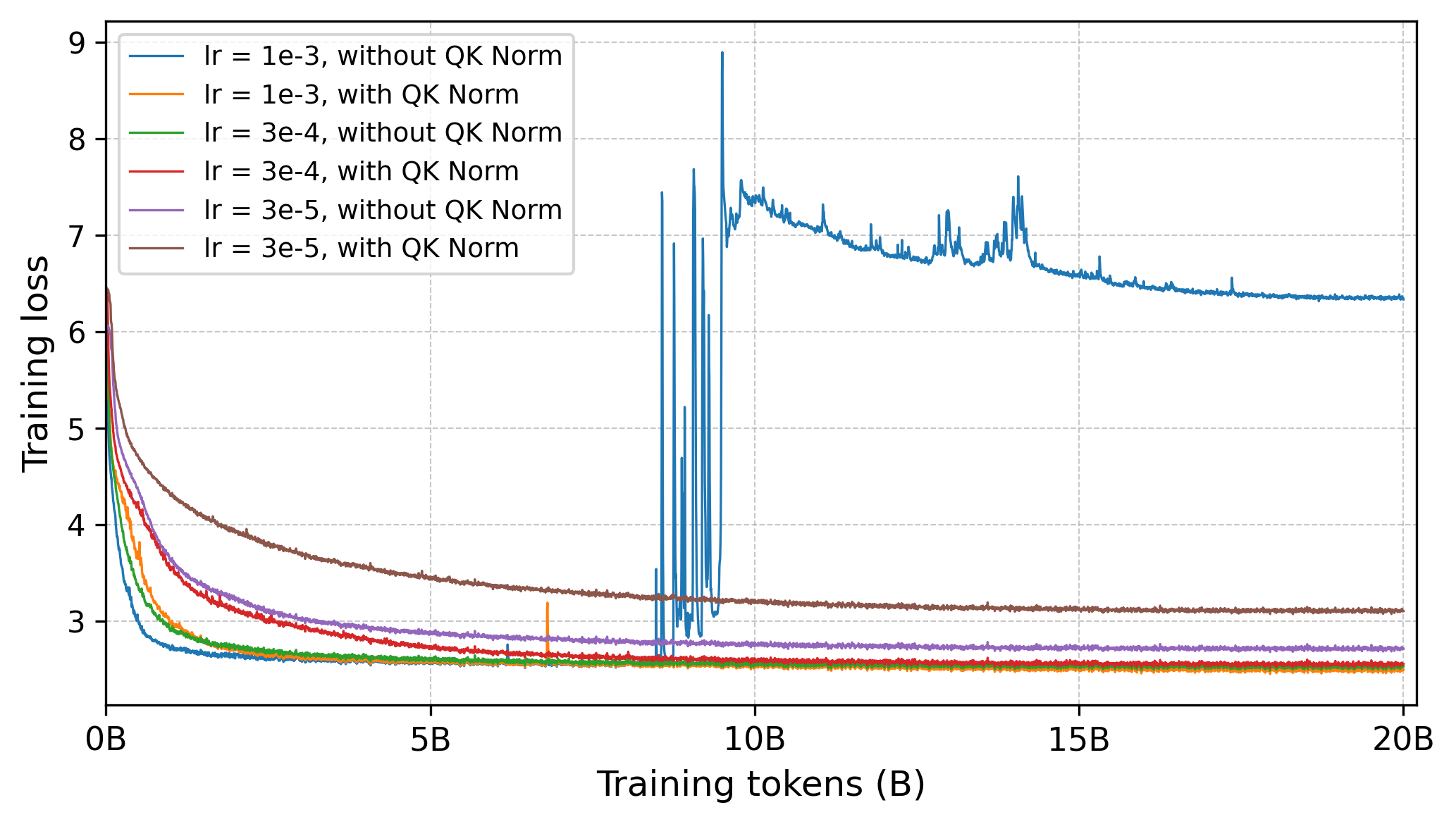
To assess the interaction between QK Norm and DroPE, we conducted a controlled ablation study on the SmolLM-360M model using six configurations: three learning rates (

3×10−53\times10^{-5}

3×10−43\times10^{-4}

10^{-3}

), each trained with and without QK Norm. The results, summarized in Table 11, yield two main observations:

Lower learning rates ( $3×10−53\times10^{-5}$ , $3×10−43\times10^{-4}$ ). DroPE works effectively without QKNorm. At the lowest learning rate ( $3×10−53\times10^{-5}$ ), the model without QK Norm achieves a slightly better final loss ( $2.713$ vs. $3.102$ ). Together with the $3×10−43\times10^{-4}$ setting ( $2.530$ vs. $2.555$ ), this indicates that QK Norm does not consistently improve performance in low-volatility regimes and is not the source of our gains.
High learning rate ( $10^{-3}$ ). At the highest learning rate, the model without QKNorm becomes unstable (loss spikes, gradient explosions), leading to poor convergence (final loss 6.334). In contrast, adding QKNorm stabilizes training and allows us to leverage the higher learning rate to achieve the best overall performance (final loss 2.496).

Figure 12 shows the corresponding training curves with and without QK Norm, highlighting the presence of loss spikes at higher learning rates, in line with observations reported in [58]. These results empirically demonstrate that the primary role of QK Norm is to act as a stabilizer that enables the use of a more aggressive, compute-efficient learning rate. Importantly, DroPE can still be applied without QK Norm by using a moderate learning rate (e.g., (

3×10−43\times10^{-4}

), which is our default setting for all experiments except the longer SmolLM-360M recalibration phases.

Table 11: Ablation study on SmolLM-360M recalibration with and without QK Norm across different learning rates.

Learning Rate	With QK Norm	Without QK Norm	Status
$10^{-3}$ (High)	$2.496$	$6.334$	Unstable without Norm
$3\times10^{-4}$ (Mid)	$2.555$	$2.530$	Stable / Comparable
$3\times10^{-5}$ (Low)	$3.102$	$2.713$	Stable / Comparable

References

[1] Brown et al. (2020). Language models are few-shot learners. Advances in neural information processing systems. 33. pp. 1877–1901.

[2] Team et al. (2023). Gemini: a family of highly capable multimodal models. arXiv preprint arXiv:2312.11805.

[3] (2021). Highly accurate protein structure prediction with AlphaFold. nature. 596(7873). pp. 583–589.

[4] Dosovitskiy et al. (2020). An image is worth 16x16 words: Transformers for image recognition at scale. arXiv preprint arXiv:2010.11929.

[5] Vaswani et al. (2017). Attention is all you need. Advances in neural information processing systems. 30.

[6] Dao et al. (2022). Flashattention: Fast and memory-efficient exact attention with io-awareness. Advances in neural information processing systems. 35. pp. 16344–16359.

[7] Liu et al. (2023). Ring attention with blockwise transformers for near-infinite context. arXiv preprint arXiv:2310.01889.

[8] Liu, Hao and Abbeel, Pieter (2023). Blockwise parallel transformers for large context models. Advances in neural information processing systems. 36. pp. 8828–8844.

[9] Press et al. (2021). Train short, test long: Attention with linear biases enables input length extrapolation. arXiv preprint arXiv:2108.12409.

[10] Chi et al. (2023). Attention alignment and flexible positional embeddings improve transformer length extrapolation. arXiv preprint arXiv:2311.00684.

[11] Su et al. (2024). Roformer: Enhanced transformer with rotary position embedding. Neurocomputing. 568. pp. 127063.

[12] Chen et al. (2023). Extending context window of large language models via positional interpolation. arXiv preprint arXiv:2306.15595.

[13] bloc97 (2023). NTK-Aware Scaled RoPE allows LLaMA models to have extended (8k+) context size without any fine-tuning and minimal perplexity degradation. Reddit post on r/LocalLLaMA. Accessed: 2025-09-19. https://www.reddit.com/r/LocalLLaMA/comments/14lz7j5/ntkaware_scaled_rope_allows_llama_models_to_have/.

[14] Peng et al. (2023). Yarn: Efficient context window extension of large language models. arXiv preprint arXiv:2309.00071.

[15] Ding et al. (2024). Longrope: Extending llm context window beyond 2 million tokens. arXiv preprint arXiv:2402.13753.

[16] Lu et al. (2024). A controlled study on long context extension and generalization in llms. arXiv preprint arXiv:2409.12181.

[17] Choromanski et al. (2020). Rethinking attention with performers. arXiv preprint arXiv:2009.14794.

[18] Wang et al. (2020). Linformer: Self-attention with linear complexity. arXiv preprint arXiv:2006.04768.

[19] Xiong et al. (2021). Nyströmformer: A nyström-based algorithm for approximating self-attention. In Proceedings of the AAAI conference on artificial intelligence. pp. 14138–14148.

[20] Zaheer et al. (2020). Big bird: Transformers for longer sequences. Advances in neural information processing systems. 33. pp. 17283–17297.

[21] Kazemnejad et al. (2023). The impact of positional encoding on length generalization in transformers. Advances in Neural Information Processing Systems. 36. pp. 24892–24928.

[22] Yang et al. (2025). Rope to nope and back again: A new hybrid attention strategy. arXiv preprint arXiv:2501.18795.

[23] Puvvada et al. (2025). Swan-gpt: An efficient and scalable approach for long-context language modeling. arXiv preprint arXiv:2504.08719.

[24] Yi Lu et al. (2024). A Controlled Study on Long Context Extension and Generalization in LLMs. https://arxiv.org/abs/2409.12181.

[25] Haviv et al. (2022). Transformer language models without positional encodings still learn positional information. arXiv preprint arXiv:2203.16634.

[26] Liu et al. (2023). Lost in the middle: How language models use long contexts. arXiv preprint arXiv:2307.03172.

[27] Greg Kamradt (2023). Needle In A Haystack — Pressure Testing LLMs. https://github.com/gkamradt/LLMTest_NeedleInAHaystack. GitHub repository.

[28] Cheng-Ping Hsieh et al. (2024). RULER: What's the Real Context Size of Your Long-Context Language Models?. arXiv preprint arXiv:2404.06654. doi:10.48550/arXiv.2404.06654. https://arxiv.org/abs/2404.06654.

[29] (2024). Round and round we go! what makes rotary positional encodings useful?. arXiv preprint arXiv:2410.06205.

[30] (2024). The fineweb datasets: Decanting the web for the finest text data at scale. Advances in Neural Information Processing Systems. 37. pp. 30811–30849.

[31] Hoffmann et al. (2022). Training compute-optimal large language models. arXiv preprint arXiv:2203.15556.

[32] Loubna Ben Allal et al. (2024). SmolLM - blazingly fast and remarkably powerful.

[33] Henry et al. (2020). Query-key normalization for transformers. arXiv preprint arXiv:2010.04245.

[34] OLMo et al. (2024). 2 OLMo 2 Furious. arXiv preprint arXiv:2501.00656.

[35] Yushi Bai et al. (2023). LongBench: A Bilingual, Multitask Benchmark for Long Context Understanding. arXiv preprint arXiv:2308.14508. doi:10.48550/arXiv.2308.14508. https://arxiv.org/abs/2308.14508.

[36] Clark et al. (2018). Think you have solved question answering? try arc, the ai2 reasoning challenge. arXiv preprint arXiv:1803.05457.

[37] Zellers et al. (2019). Hellaswag: Can a machine really finish your sentence?. arXiv preprint arXiv:1905.07830.

[38] Mihaylov et al. (2018). Can a suit of armor conduct electricity? a new dataset for open book question answering. arXiv preprint arXiv:1809.02789.

[39] Bisk et al. (2020). Piqa: Reasoning about physical commonsense in natural language. In Proceedings of the AAAI conference on artificial intelligence. pp. 7432–7439.

[40] Sakaguchi et al. (2021). Winogrande: An adversarial winograd schema challenge at scale. Communications of the ACM. 64(9). pp. 99–106.

[41] Touvron et al. (2023). Llama 2: Open foundation and fine-tuned chat models. arXiv preprint arXiv:2307.09288.

[42] Ermo Hua et al. (2025). Fourier Position Embedding: Enhancing Attention’s Periodic Extension for Length Generalization. In Forty-second International Conference on Machine Learning. https://openreview.net/forum?id=ZfDNDkg7Dh.

[43] Yui Oka et al. (2025). Wavelet-based Positional Representation for Long Context. In The Thirteenth International Conference on Learning Representations. https://openreview.net/forum?id=OhauMUNW8T.

[44] (2025). Round and Round We Go! What makes Rotary Positional Encodings useful?. In The Thirteenth International Conference on Learning Representations. https://openreview.net/forum?id=GtvuNrk58a.

[45] zican Dong et al. (2024). Exploring Context Window of Large Language Models via Decomposed Positional Vectors. In The Thirty-eighth Annual Conference on Neural Information Processing Systems. https://openreview.net/forum?id=zeYyq0GpXO.

[46] Tong Wu et al. (2024). An Efficient Recipe for Long Context Extension via Middle-Focused Positional Encoding. In The Thirty-eighth Annual Conference on Neural Information Processing Systems. https://openreview.net/forum?id=aNHEqFMS0N.

[47] Chuanyang Zheng et al. (2024). DAPE: Data-Adaptive Positional Encoding for Length Extrapolation. In The Thirty-eighth Annual Conference on Neural Information Processing Systems. https://openreview.net/forum?id=rnUEUbRxVu.

[48] Vershynin, Roman (2018). High-dimensional probability: An introduction with applications in data science. Cambridge university press.

[49] Nesterov, Yurii (2013). Introductory lectures on convex optimization: A basic course. Springer Science & Business Media.

[50] Yang et al. (2024). Qwen2 technical report, 2024. URL https://arxiv. org/abs/2407.10671. 7. pp. 8.

[51] Loshchilov, Ilya and Hutter, Frank (2017). Decoupled weight decay regularization. arXiv preprint arXiv:1711.05101.

[52] Ben Allal et al.. SmolLM-Corpus. https://huggingface.co/datasets/HuggingFaceTB/smollm-corpus.

[53] Radford et al. (2019). Language models are unsupervised multitask learners. OpenAI blog. 1(8). pp. 9.

[54] Wang et al. (2024). Length generalization of causal transformers without position encoding. arXiv preprint arXiv:2404.12224.

[55] (2023). LightEval: A lightweight framework for LLM evaluation. https://github.com/huggingface/lighteval.

[56] Shang et al. (2025). LongRoPE2: Near-Lossless LLM Context Window Scaling. arXiv preprint arXiv:2502.20082.

[57] Yang et al. (2025). Qwen3 technical report. arXiv preprint arXiv:2505.09388.

[58] OLMo et al. (2024). 2 OLMo 2 Furious. arXiv preprint arXiv:2501.00656.

Method	Avg. LongBench score
SmolLM	2.59
SmolLM + PI	2.48
SmolLM + RoPE-NTK	12.21
SmolLM + YaRN	13.07
SmolLM- DroPE	13.81