Hilbert Operator for Progressive Encoding (HOPE): A Mathematical Framework for Deconstructing Learned Representations in Deep Networks

Hossein Mobahi$^{1}$, Peter L. Bartlett$^{1,2}$

$^{1}$ Google Research
$^{2}$ University of California, Berkeley

Abstract

Deep neural networks encode complex representations, but deconstructing this internal knowledge remains a challenge. Given the link between learning and compression, network compression offers a promising lens to analyze this knowledge. However, standard compression heuristics often suffer from scale symmetries and architectural biases. To resolve these, we introduce Hilbert Operator for Progressive Encoding (HOPE), a mathematical framework to gradually deconstruct the representations in trained network weights.

HOPE shifts network compression from the discrete domain into a Hilbert space of continuous functions. By modeling individual neurons as rank-1 Hilbert-Schmidt operators, HOPE unifies pruning and neuron merging as low-rank subspace projection. Extending this formulation, HOPE introduces macro block eviction to encompass multi-layer structures like entire residual pathways under the same unified metric. This unified approach enables unbiased architectural decisions across layers with different types and sizes. HOPE is a data-free and hyperparameter-free framework. We present proof-of-concept experiments in model compression and fine-tuning to highlight the practical potential of our theory.

Correspondence: [email protected], [email protected]

Executive Summary: Deep neural networks learn powerful but opaque internal representations, and extracting or reducing their capacity after training remains difficult. Standard compression techniques often rely on raw parameter magnitudes that are distorted by optimization artifacts, require repeated passes over data, or introduce architectural biases that favor certain layers or neuron shapes. These issues hinder objective analysis of what networks have truly learned, limit reliable model compression, and complicate transfer to new tasks without erasing prior knowledge. Because learning itself has deep connections to compression, progressive capacity reduction offers a measurable way to separate stable core features from malleable peripheral ones.

The document introduces HOPE, a mathematical framework that shifts compression analysis from discrete parameter space into a continuous function space. It models each neuron as a rank-1 operator in a Hilbert space, where importance and similarity are evaluated via functional norms and inner products rather than raw weights. For networks with batch normalization, the method derives a data-free Gaussian surrogate from existing statistics; otherwise it needs only a single small calibration pass. This unified view treats pruning, neuron merging, and eviction of entire residual blocks as instances of the same low-rank projection operation, all decided by a single, hyperparameter-free cost that balances distortion against parameter reduction.

Proof-of-concept experiments on a pretrained ResNet-50 show that HOPE produces compressed models with higher accuracy at a given density than magnitude-based structured pruning baselines. In cross-domain transfer from CIFAR-100 variants to SVHN, a fine-tuning procedure built on HOPE (called DEFT) retains substantially more source-task performance while matching most of the target-task gains of full fine-tuning, yielding a markedly higher combined score than head-only tuning, elastic weight consolidation, or batch-norm-only plasticity.

These results matter because they provide a principled, largely data-free route to model size reduction and to controlled adaptation that protects previously learned invariants. The same machinery could support interpretability work and continual learning by explicitly exposing which parts of a network encode reusable abstractions versus task-specific slack.

Next steps should include scaling the approach to larger models and transformer architectures, testing on additional downstream tasks, and exploring whether the identified core-periphery partition improves robustness or safety properties. A modest pilot on one additional domain would clarify whether the observed transfer gains hold beyond the reported settings.

The main limitations are that the work presents only proof-of-concept results rather than exhaustive benchmarks, relies on certain modeling assumptions such as Gaussian pre-activations, and has so far been validated primarily on convolutional networks with batch normalization. Confidence is therefore moderate: the theoretical construction is consistent and the reported gains are clear, yet broader empirical validation is still required before strong deployment decisions.

1. Introduction

Section Summary: The paper argues that model compression offers an objective way to study the hidden knowledge inside deep neural networks by progressively stripping away unnecessary parts, revealing the stable core patterns the network has learned. It notes that common pruning methods based on weight size or real data often fail or become unreliable, so the authors introduce the HOPE framework, which instead analyzes each neuron as a mathematical operator in a continuous function space. This approach enables fully data-free, hyperparameter-free compression that works by using built-in network statistics to measure importance without repeated dataset evaluations.

While deep neural networks learn complex representations, deconstructing this knowledge from numerical weights remains challenging. In this work, we use model compression as a measurable proxy task to study these internal representations objectively. Given the fundamental link between compression and learning [1, 2], which has recently been reinforced by demonstrating that LLMs are general-purpose compressors [3] and amortized algorithmic predictors [4], we believe compression provides a promising lens to study this issue objectively. Deconstructing opaque networks through capacity reduction has foundational roots [5]. Viewed through a modern information-theoretic lens, learning is essentially the systematic discarding of task-irrelevant noise to isolate generalizable core patterns [6, 7].

Consequently, we posit that progressive compression is an effective tool for achieving this separation. Because core invariants resist pruning significantly longer than malleable slack, iteratively reducing capacity with minimal distortion naturally peels away the periphery to expose the network's universal feature space [8, 9, 10]. This post-training deconstruction mirrors the network's learning dynamics: the "coarse-graining" dimensionality reduction that gradient descent originally used to build them [11]. Indeed, theoretical analyses confirm that networks learn by incrementally adding effective units to model increasingly complex functions [12]. While biologically inspired paradigms like [13] achieve this core-slack segregation by expanding a network to consolidate memories, we demonstrate that this separation can be accomplished efficiently through data-free compression.

Despite compression's promise, the opacity of deep networks poses hurdles for objectively identifying and reducing capacity. Simple heuristics such as magnitude-based pruning (e.g. norm of raw weights) often fail because these magnitudes are typically optimization artifacts rather than importance indicators [14, 15, 16], as also long observed in network sparsification [17, 18, 19].

To address the shortcomings of magnitude based notions of capacity, we propose to transition from the physical parameter space to the function space, specifically the underlying transformation a neuron applies to its input. This perspective treats the entire neuron, rather than individual weight matrices, as the atomic unit of the network. Note that this transformation must be analyzed over the relevant data manifold rather than the entire input space. For instance, characterizing a neuron's behavior within a dog-versus-cat image classification task requires isolating the data manifold specific to those two classes, while discarding irrelevant classes and non-natural images. While one might attempt to approximate the input manifold to each neuron empirically by passing a finite dataset through the network, such finite-dimensional approximations tether the evaluation to specific samples. This reliance on explicit data sets can render the resulting architecture brittle to distribution shifts and disproportionately degrade performance on long-tail features [16]. Furthermore, empirical approaches that rely on continuous activation matching or curvature approximations [20, 21] incur a severe computational penalty, as they require numerically evaluating neural activations across the dataset repeatedly during every iteration of the progressive model encoding.

To avoid both the drawbacks of weight-based parameterization and the pitfalls of empirical data dependence, we introduce the Hilbert Operator for Progressive Encoding (HOPE) framework. The core philosophy of HOPE is that evaluation and analysis of neurons must occur in the function space, the resulting compression must be executed discretely on the network's parameters. By lifting the parameter vectors and matrices of individual neurons into continuous functions, HOPE models each neuron as a rank-1 Hilbert-Schmidt operator. This abstraction unifies pruning and merging under a single theoretical paradigm: an optimal low-rank projection within a functional tensor space, where distances are measured by $\left\lVert \cdot\right\rVert_{\mathcal{H}}$. Once the optimal reductions (pruning or merging) are computed in this pure functional space, the framework projects the resulting continuous operators back onto the network parameters to execute the compression.

A key advantage of HOPE is that it operates entirely data-free for networks utilizing Batch Normalization (BN).[^2] While prior research has successfully exploited BN moving averages to generate synthetic images for data-free knowledge distillation [22, 23], HOPE leverages this information in a different manner. Instead of generating synthetic spatial data or relying on massive real datasets to drive input signals, HOPE applies the Maximum Entropy principle directly to the empirical BN statistics embedded within the trained model checkpoint. This yields a continuous surrogate for the local input distribution at each neuron, allowing the framework to analytically evaluate the integrals required for Hilbert space norms $\left\lVert \cdot\right\rVert_{\mathcal{H}}$. This fully continuous, analytical perspective largely mitigates scaling symmetries inherent in raw parameters, and thus enables unbiased capacity measurements across heterogeneous layers without requiring a single real or synthetic data sample.

[^2]: This data-free approach relies on global BN statistics. For architectures lacking BN, HOPE easily adapts: it requires only a simple, one-time calibration pass over a small data batch to capture the necessary pre-activation statistics.

The primary value of HOPE lies in establishing a rigorous, hyperparameter free (and also data free in presence of BN) mathematical framework for the progressive encoding of trained deep networks. We present proof-of-concept applications for model compression and fine-tuning experiments to empirically validate these theoretical capabilities, rather than to establish exhaustive, large-scale benchmarks.

Paper Organization.

We begin with a literature review in Section 2 and formally define a neuron within our framework in Section 3. To enable data-free evaluation, Section 4 constructs a surrogate distribution constrained by Batch Normalization (BN) statistics. In Section 5, we lift discrete neurons into continuous Hilbert-Schmidt operators. Section 6 then derives a cost functional $\mathcal{J}$ that captures the distortion induced by pruning or merging via subspace projection. Building on this, Section 7 derives the optimal parent neuron in function space for a given pair of merged neurons, detailing how this continuous representation is mapped back to the network's discrete parameters. Section 8 extends this projection metric to the macro level to evict larger residual blocks. Section 9 introduces a rate-distortion-inspired objective that balances the distortion cost $\mathcal{J}$ against the resulting reduction in parameter count; this objective is used to greedily select the next optimal compression action. Section 10 presents the encoding process as a loop over greedy selection of compression actions. Finally, Section 11 provides a proof-of-concept evaluation of our framework for model compression and fine-tuning.

2. Related Works

Section Summary: Existing work on neural network compression has relied on pruning weights or neurons based on their magnitudes or activation patterns, along with techniques for merging similar neurons and selectively dropping layers, but these methods often require running data through the model, suffer from unreliable importance estimates, or treat pruning and merging as separate steps. Related efforts in data-free compression generate synthetic inputs or use statistical shortcuts, while research on continual learning explores how to protect core knowledge from being overwritten during updates. HOPE seeks to address the shortcomings of these approaches by evaluating neuron importance through projections in a continuous functional space, enabling unified, data-free pruning, merging, and architectural reduction without relying on parameter magnitudes or repeated dataset passes.

Pruning and Parameter-Space Methods. Network compression has historically relied on parameter-space pruning, evolving from early Taylor-expansion techniques [17, 18] to modern unstructured [24, 19] and structured [25, 26] approaches. HOPE directly compares against structured baselines utilizing $L_1$-norms [27] and BN scaling [28]. To capture functional importance, methods ranging from early skeletonization via error derivatives [5] to modern empirical activation tracking [20, 29, 30, 21] rely on dataset passes; however, this introduces computational bottlenecks and brittleness to distribution shifts [16]. Conversely, parameter-centric heuristics suffer from "scale symmetry" [31, 32, 33, 34], where overparameterized many-to-one mappings [35] mean raw magnitudes often reflect optimization artifacts rather than true importance [14, 15, 16]. Although methods like [36] can partially mitigate global scale symmetries, they remain bound to parameter-space magnitude heuristics, which are vulnerable to within-neuron scaling artifacts. By migrating evaluation to a continuous Hilbert space, HOPE circumvents both empirical data bottlenecks and parameter-space artifacts. This shift from structural to functional mappings aligns with the Platonic Representation Hypothesis [37], which posits that diverse networks converge to a shared statistical model of reality, treating weight spaces as mere shadows. HOPE operationalizes this intra-model, defining identity via continuous operators rather than superficial parameters.

Neuron Alignment and Model Merging. Some recent methods on merging networks include permutation invariances [38, 39], Optimal Transport [40], alignment strategies [41], or feature zipping [42]. Other approaches perform data-free neuron merging by evaluating pairwise parameter similarities [43] or clustering weights via adaptive scalar hashing [44]. However, these methods typically rely on combinatorial matching or parameter averaging. HOPE advances this paradigm by unifying pruning and merging under a single continuous operation: optimal low-rank projection in a functional tensor space, penalizing distortion via the Hilbert-Schmidt norm. This geometric approach mirrors using subspace embeddings to capture hierarchical and compositional representations [45]. Merging acts as the inverse to "feature splitting" [46] or computation in superposition [47], where overparameterized models fragment concepts across correlated sub-features, a phenomenon rooted in foundational vector space arithmetic [48, 49] and the Linear Representation Hypothesis [50, 51]. By projecting a rank-2 neuron pair into an optimal rank-1 Hilbert-Schmidt parent, HOPE reconsolidates this distributed knowledge, reclaiming capacity while preserving the network's underlying linear geometry.

Macro Architecture and Layer Pruning. To reduce network's depth, standard methods employ stochastic depth [52], heuristic layer dropping [53], Neural Architecture Search [54, 55], or dynamic routing gates [56, 57]. However, these approaches decouple macro-architectural decisions from granular feature selection, relying on separate optimization phases or custom hyperparameters. HOPE unifies these scales by formalizing block eviction as a macroscopic function subspace projection. Mapping this architectural deletion to the identical capacity cost $\mathcal{J}$ allows macro-reductions to compete against granular pruning and merging within a single, hyperparameter-free decision engine.

Data-Free Compression and Maximum Entropy Surrogates. Bypassing the original training data often involves inverting BN statistics to generate synthetic inputs [58, 59, 60, 23, 22] or conserving discrete synaptic flow at initialization [15]. Rather than generating explicit samples, HOPE elevates these empirical statistics via the Maximum Entropy principle [61] to construct a continuous analytical surrogate, similar to some task-agnostic pruning of LLMs [62]. Paralleling theoretical analyses of infinite-width networks and Gaussian Processes [63, 64, 65, 66], this framework allows infinite-dimensional integrals to be resolved without a single forward pass.

Parameter Plasticity, Continual Learning, and Representation Deconstruction. HOPE conceptually bridges progressive compression with transfer learning [67, 68, 69] and the Stability-Plasticity dilemma of continual learning [70, 71, 72]. Drawing parallels to Complementary Learning Systems in cognitive neuroscience [73, 74], and aligning with the growing recognition across deep learning [75], we hypothesize that the learned representation must be explicitly segregated into a universal core of invariants and a peripheral slack of malleable volume in order to allow learning without forgetting. While previous frameworks attempt to protect foundational knowledge against representational drift using computationally massive $\mathcal{O}(N^3)$ orthogonal matrix projections [76, 77, 78, 79] or dataset-dependent quadratic penalties [71], HOPE provides a purely data-free alternative. By computing neuron capacity in $\mathcal{O}(N)$ time, its progressive pruning and merging peel away slack and expose core abstractions, computationally mirroring how awake biological circuits rapidly decorrelate co-activated neurons to maintain network stability [80]. This perspective is corroborated by recent literature utilizing capacity reduction to deconstruct hierarchies. For example, targeted parameter removal has been used to explain robustness [8], uncover heavy-tailed synaptic backbones [9], and demonstrate hierarchical learning through progressive feature compression [10]. Collectively, these works support the premise that HOPE's neuron capacity may efficiently identify foundations versus plastic slack, laying the groundwork for transfer learning and downstream algorithmic interpretability [81, 82, 83, 84].

3. The Neuron

Section Summary: The section argues that scale symmetries in neural networks are best understood at the level of an entire neuron, which bundles its input weights, batch-norm parameters, activation function, and output weights into one functional unit. It absorbs the normalization step into “effective” input weights and a bias term so that the neuron’s overall mapping from input to downstream contribution depends only on the normalized pre-activation signal. By working with these adjusted parameters rather than the raw weights, the framework removes the misleading effects of normalization invariance and ensures that any measure of a neuron’s capacity reflects its actual functional behavior.

Scale invariances are inherently relational and that is why isolated parameters fail to capture them. The minimal architectural unit where these symmetries fully manifest is the neuron in its entirety (encapsulating its incoming weights, BN parameters, non-linear activation, and outgoing weights). In this section we discuss how these within-neuron scale symmetries can be factored out, while deferring global scale symmetries to Section 5. For clarity, we derive our theoretical framework under the assumption of a fully connected architecture. However, this formalism seamlessly extends to convolutional networks (see Appendix B.1). Indeed, the architectures evaluated in Section 11 rely on this adaptation.

Consider a neuron $i$ with input weights $\boldsymbol{w}{\text{raw}, i} \in \mathbb{R}^n$ and output weights $\boldsymbol{w}{\text{out}, i} \in \mathbb{R}^c$. Let the neuron be subject to learnable affine BN parameters $(\gamma_i, \beta_i)$ and empirical moving dataset statistics $(\mu_i, \sigma_i^2)$, where $\mu_i \triangleq \mathbb{E}{\mathcal{X}}[\boldsymbol{w}{\text{raw}, i}^T \boldsymbol{x}]$ and $\sigma_i^2 \triangleq \operatorname{Var}{\mathcal{X}}(\boldsymbol{w}{\text{raw}, i}^T \boldsymbol{x})$. To capture the signal reaching the non-linearity, we absorb the normalization operations into a set of effective parameters:

$ \boldsymbol{w}{\text{in}, i}^{\text{eff}} , \triangleq, \gamma_i/\sqrt{\sigma_i^2 + \epsilon} \boldsymbol{w}{\text{raw}, i} \qquad, \qquad b_i , \triangleq, \beta_i - \gamma_i \mu_i/\sqrt{\sigma_i^2 + \epsilon} , ,\tag{1} $

where $\epsilon > 0$ is a small numerical stability constant. The neuron's end-to-end signal mapping, capturing its functional contribution to the subsequent layer for an input $\boldsymbol{x}$, is defined by the continuous function:

$ f_i(\boldsymbol{x}) = \Psi(y_i) \boldsymbol{w}{\text{out}, i} \qquad, \qquad y_i \triangleq (\boldsymbol{w}{\text{in}, i}^{\text{eff}})^T \boldsymbol{x} + b_i , ,\tag{2} $

where $\Psi(\cdot)$ denotes a PH-1 activation function defined as below:

Throughout the HOPE framework, we formally designate this continuous function $f_i$ as the neuron. Operating at this atomic level mitigates two primary sources of scaling symmetry: normalization invariance (from BN) and re-parameterization invariance (from cross-layer weight resharding). We detail the former below, and defer the latter to Section 5.

3.1 Mitigating Normalization Invariance

Normalization invariance arises from BN's standardizing mechanics. Scaling raw input weights $\boldsymbol{w}_{\text{raw}, i}$ by a constant factor $\lambda > 0$ increases the pre-activation variance by $\lambda^2$. The subsequent BN layer divides by the standard deviation, canceling $\lambda$ before the non-linearity. Because downstream output remains unchanged, raw weight magnitudes can be deceptive.

HOPE mitigates this failure mode by evaluating capacity through effective parameters ($\boldsymbol{w}{\text{in}, i}^{\text{eff}}$ and $b_i$). While HOPE uses raw weights $\boldsymbol{w}{\text{raw}, i}$ alongside BN statistics to construct the data-constrained surrogate dataset $P_{\mathcal{X}}$ (Section 4), their utility ends there. The framework then evaluates the neuron's continuous-functional impact on this surrogate.

Physically, the non-linear activation processes the normalized, shifted signal, not the raw parameter projection. Thus, when computing the continuous integral to compute Hilbert space norms or inner product, HOPE defines the pre-activation signal as $y_i = (\boldsymbol{w}{\text{in}, i}^{\text{eff}})^T \boldsymbol{x} + b_i$. Because $\boldsymbol{w}{\text{in}, i}^{\text{eff}}$ divides by the empirical standard deviation $\sigma_i$, any magnitude inflation is canceled. By evaluating the signal impacting the activation function, HOPE guarantees the capacity criterion reflects functional utility rather than scale artifacts.

4. The Neural Signal Distribution

Section Summary: Since HOPE lacks access to the true data distribution, it constructs a Gaussian surrogate using the maximum entropy principle and statistics from batch normalization layers. This works because each neuron effectively sees its inputs only through high-dimensional linear projections, which converge to Gaussian signals by the central limit theorem across layers even if the original data manifold is complex. The resulting multivariate Gaussian matches the observed per-neuron means and variances through an optimal least-squares mean and a constrained covariance that can be handled efficiently via low-rank pairwise merges.

Since HOPE operates in a data-free regime, the true input distribution $P^*_{\mathcal{X}}$ (encompassing both initial data and subsequent layer activations) is inaccessible. However, because we model neurons as continuous Hilbert-Schmidt operators, evaluating their inner products requires integrating over the data distribution. To resolve this, we invoke the Maximum Entropy principle [61] to construct a Gaussian surrogate constrained by BN statistics. While a Gaussian approximation may seem overly idealistic, we explain below in two steps why it aligns closely with modern neural architectures.

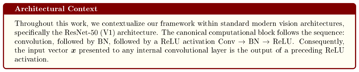
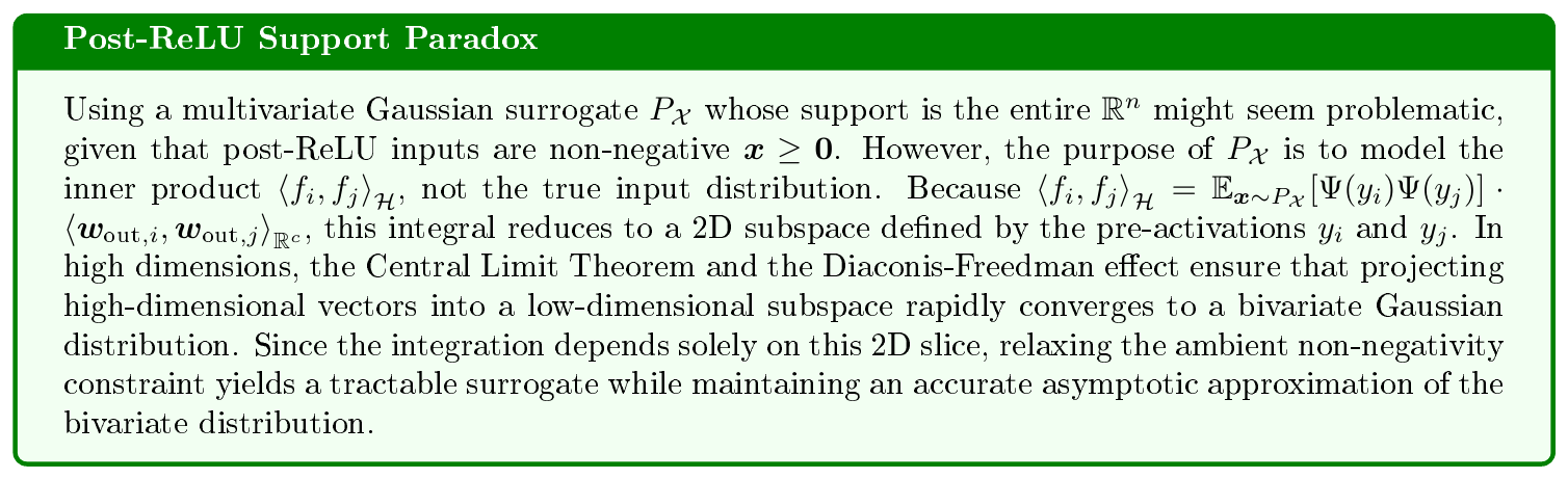
Step 1: Gaussianity of Pre-Activation. While a neuron's true input distribution $P^*_{\mathcal{X}}$ often lies on a complex, highly non-Gaussian manifold, each neurons observes its input $\boldsymbol{x}$ only through 1-dimensional linear projections $y = \sum_{j=1}^{n} w_j x_j$. As the fan-in dimension $n$ grows, by the Central Limit Theorem and the Diaconis-Freedman effect [85], these aggregated signals converge to a Gaussian distribution. Consequently, neurons remain oblivious to the complex data manifold; from their perspective the pre-activation $y_i$ is Gaussian. Although nonlinear activations (e.g., ReLU) disrupt this Gaussianity, subsequent high-dimensional linear transformations recursively smooth the signals back into Gaussian pre-activations across layers.

Step 2: Gaussian Surrogate for the Input $\boldsymbol{x}$. While neurons are oblivious to the true shape of the data manifold and perceive their input as a Gaussian signal $y$. Based on this observation, for theoretical convenience, we substitute the complex true data with a tractable surrogate. For architectural consistency, the surrogate distribution must satisfy the same observational bottleneck: its 1D linear projections must remain Gaussian. By definition, if every linear combination of a random vector is Gaussian, the vector itself must be multivariate Gaussian. Thus, to construct a surrogate distribution aligned with a world where every linear observer (neuron) sees a Gaussian, that surrogate is necessarily a multivariate Gaussian, $P_{\mathcal{X}} = \mathcal{N}(\hat{\boldsymbol{\mu}}_x, \hat{\Sigma}_x)$.

Optimal Surrogate. To define the optimal parameters $(\hat{\boldsymbol{\mu}}x, \hat{\Sigma}x)$ of the unknown data distribution, we can incorporate the two empirical constraints $\boldsymbol{x} \in \mathbb{R}^n$: $\mathbb{E}[\boldsymbol{w}{\text{raw}, i}^T \boldsymbol{x}] = \mu_i$ and $\operatorname{Var}(\boldsymbol{w}{\text{raw}, i}^T \boldsymbol{x}) = \sigma_i^2$ imposed by BN for any $i$. We define a shared surrogate for each layer. Since the empirical means $\boldsymbol{\mu}{\text{BN}} \in \mathbb{R}^n$ represent the 1D shadow of the dataset's center cast through the raw weights, to find the best mean for a layer we compute the optimal least-squares approximation of the dataset's center using the Moore-Penrose pseudo-inverse $\boldsymbol{W}{\text{raw}}^+$, which leads to $\hat{\boldsymbol{\mu}}x = \boldsymbol{W}{\text{raw}}^+ \boldsymbol{\mu}{\text{BN}}$. In underdetermined scenarios (e.g., when compressing layers where $n > c$), this pseudo-inverse yields the minimum-norm solution, which sets the unobserved orthogonal components of the data manifold to a zero mean. To find the optimal covariance matrix $\hat{\Sigma}x$ for the layer, we maximize the differential entropy of the multivariate Gaussian, $H(\boldsymbol{x}) \propto \log \det(\Sigma_x)$ subject to the BN variance constraints $\boldsymbol{w}{\text{raw}, i}^T \Sigma_x \boldsymbol{w}{\text{raw}, i} = \sigma_i^2$ for $i \in {1, \dots, c}$. Conceptually, applying Lagrange multipliers yields $\hat{\Sigma}x = \left(\sum{i=1}^c \lambda_i \boldsymbol{w}{\text{raw}, i} \boldsymbol{w}{\text{raw}, i}^T \right)^{-1}$, where $\lambda_i$ are optimized to satisfy variance equality constraints. However, inverting this covariance matrix is computationally expensive. Fortunately, the framework bypasses the computationally expensive need to compute and invert the full high-dimensional joint covariance matrix entirely: micro-operations evaluate pairwise merges restricted to a rank-2 subspace, allowing a closed-form solution via a pairwise neural kernel (Appendix E.3), while macro block eviction evaluates destruction using the $L_1$ cumulative distance of surviving capacities (Section 8).

5. A Hilbert Functional Perspective on Neurons

Section Summary: The section proposes reframing each neuron as a continuous mathematical function rather than a collection of discrete weights, embedding it in a Hilbert space so its overall behavior can be assessed across an entire input distribution. This functional view abstracts away the neuron’s matrix shape, supplies a well-defined notion of its capacity or importance, and enables closed-form detection of inactive (“dead”) neurons without costly data passes. It also neutralizes misleading scale differences among weights by focusing on the invariant geometric properties of the resulting function.

To mitigate parameter shape bias and facilitate the identification of dead neurons, we transition from discrete parameter analysis to a continuous function formulation. By embedding each neuron into a Hilbert space[^3] $\mathcal{H}$ and treating it as a rank-1 Hilbert-Schmidt operator, our framework evaluates the actual function the neuron computes, effectively abstracting away its physical matrix shape. Furthermore, by integrating this continuous function over the analytically derived surrogate $P_{\mathcal{X}}$, HOPE identifies dead neurons via a closed-form expectation, bypassing the need for computationally expensive empirical forward passes over a dataset. Together, these features shift the evaluation criterion from raw parameter counts to functional capacity, quantified as the norm of the neuron's function in $\mathcal{H}$.

[^3]: See Appendix A for a brief introduction to Hilbert spaces.

We model each neuron as a rank-one Hilbert operator $f_i \in \mathcal{H}$. This way, a neuron's identity is not defined by its evaluation on a single input point $\boldsymbol{x}$, but its continuous behavior over the entire surrogate distribution $\mathcal{X}$. We quantify the capacity of the neuron by $\left\lVert f_i\right\rVert_\mathcal{H}$.

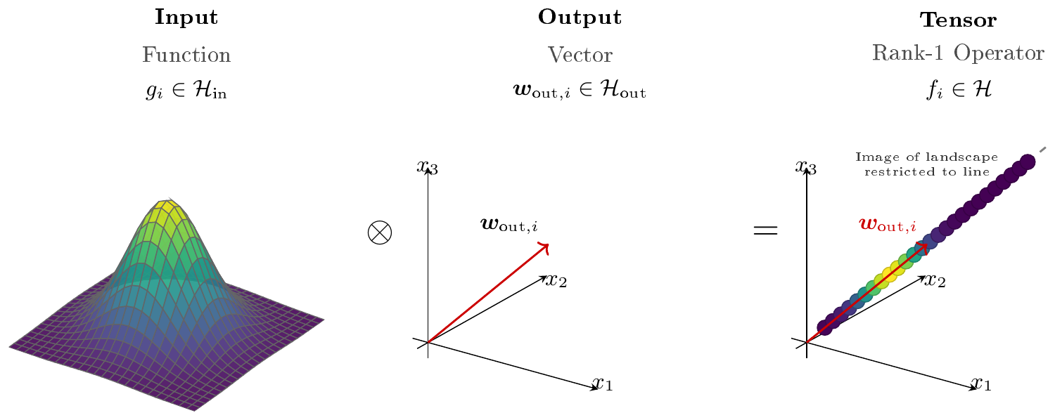
We now present this formally. We define our space of neural functions as $\mathcal{H} \triangleq L_2(\mathcal{X}, P_{\mathcal{X}}; \mathbb{R}^c)$, the space of square-integrable functions mapping $\mathcal{X}$ to the $c$-dimensional output space. Define $g_i : \mathcal{X} \rightarrow \mathbb{R}$ as $g_i(\boldsymbol{x}) \triangleq \Psi \left((\boldsymbol{w}{\text{in}, i}^{\text{eff}})^T \boldsymbol{x} + b_i \right)$. We embed $g_i$ as an element of the scalar Hilbert space $\mathcal{H}{\text{in}} \triangleq L_2(\mathcal{X}, P_{\mathcal{X}}; \mathbb{R})$. Furthermore, the scalar activation of a neuron is sent to the next layer by scaling with the finite-dimensional output weight vector $\boldsymbol{w}{\text{out}, i} \in \mathcal{H}{\text{out}} \triangleq \mathbb{R}^c$. Since the output across all $c$ dimensions is confined to the one-dimensional subspace spanned by $\boldsymbol{w}{\text{out}, i}$, this entire continuous landscape is embedded exclusively along a single vector direction. By taking the tensor product of the input function and the output vector, we construct a linear mapping across these spaces: $\mathcal{H} \cong \mathcal{H}{\text{in}} \otimes \mathcal{H}{\text{out}}$. Thus the vector-valued function $f_i : \mathcal{X} \rightarrow \mathcal{H}{\text{out}}$, i.e. the neuron, is an element within this tensor product space $f_i \triangleq g_i \otimes \boldsymbol{w}_{\text{out}, i}$. Since this element is constructed from the outer product of one input function and one output vector, each individual neuron $f_i$ is a rank-1 Hilbert-Schmidt operator. See Figure 1 for a visualization. This tensor formulation is fundamental for defining the merging operation in HOPE as we will discuss in Section 6 and Section 7.1.

Hilbert-Schmidt Inner Product and Capacity. Because our neurons are defined as rank-1 operators residing in the tensor $\mathcal{H} \cong \mathcal{H}{\text{in}} \otimes \mathcal{H}{\text{out}}$, we must evaluate their geometric relationship using the inner product defined on this composite space: $\left\langle f_i, f_j\right\rangle_{\mathcal{H}} = \left\langle g_i \otimes \boldsymbol{w}{\text{out}, i}, g_j \otimes \boldsymbol{w}{\text{out}, j}\right\rangle_{\mathcal{H}} = \left\langle g_i, g_j\right\rangle_{\mathcal{H}{\text{in}}} \cdot \left\langle \boldsymbol{w}{\text{out}, i}, \boldsymbol{w}{\text{out}, j}\right\rangle{\mathcal{H}{\text{out}}} = \mathbb{E}{\boldsymbol{x} \sim P_{\mathcal{X}}} [\Psi(y_i) \Psi(y_j)] \cdot \left\langle \boldsymbol{w}{\text{out}, i}, \boldsymbol{w}{\text{out}, j}\right\rangle_{\mathbb{R}^c}$. We define the capacity of a neuron as its Hilbert-Schmidt norm $\lVert f_i\rVert_{\mathcal{H}} = \sqrt{\left\langle f_i, f_i\right\rangle_{\mathcal{H}}}$, which we will later use to decide what neuron to prune and which macro block to evict.

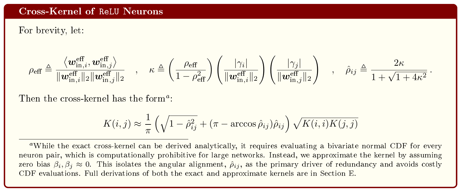
Kernel Formulation. We define the kernel of two neurons $i, j$ as $K(i, j) \triangleq \mathbb{E}{\boldsymbol{x} \sim P{\mathcal{X}}} [\Psi(y_i) \Psi(y_j)]$. Under this, the capacity of a neuron simplifies to $\lVert f_i\rVert_{\mathcal{H}} = \lVert \boldsymbol{w}{\text{out}, i}\rVert_2 \cdot \sqrt{K(i, i)}$ and the inner product of two neurons becomes $\left\langle f_i, f_j\right\rangle{\mathcal{H}} = \left\langle \boldsymbol{w}{\text{out}, i}, \boldsymbol{w}{\text{out}, j}\right\rangle_{\mathbb{R}^c} K(i, j)$. Closed form expression for these kernels are provided at the end of this section, and their derivation is presented in Appendix E when $\Psi$ is the $\texttt{ReLU}$ activation function.

Neuron Scale Invariance. In networks with PH-1 activations, scaling $\boldsymbol{w}{\text{in}, i}^{\text{eff}}$ and $b_i$ of a neuron by $\lambda>0$ and $\boldsymbol{w}{\text{out}, i}$ by $1/\lambda$ alters weight magnitudes without changing the downstream function. This symmetry confounds raw magnitude-based criteria. HOPE mitigates this issue by defining capacity as the Hilbert norm: $\lVert f_i\rVert_{\mathcal{H}} = \lVert \boldsymbol{w}_{\text{out}, i}\rVert_2 \sqrt{K(i, i)}$. Because positive homogeneity scales the kernel $K$ by $\lambda$, the opposing factors cancel. Consequently, HOPE guarantees an invariant capacity score regardless of weight resharding.

Neuron Shape Invariance. By definition, the neuron's functional capacity $|f_i|{\mathcal{H}} = | \boldsymbol{w}{\text{out}, i}|2 \sqrt{K(i, i)}$ depends on the input space $\mathcal{X}$ solely through the kernel term $K(i, i) \triangleq \mathbb{E}{\boldsymbol{x} \sim P_{\mathcal{X}}} [\Psi^2(y_i)]$. Rather than counting discrete incoming parameters $n$ or computing weight magnitudes such as $| \boldsymbol{w}{\text{in}, i}^\text{eff}|$ or $| \boldsymbol{w}{\text{raw}, i}|$, this formulation abstracts away the physical dimensionality of the input tensor $\boldsymbol{x} \in \mathbb{R}^n$.[^4] Furthermore, when paired with the layer-wise magnitude neutrality axiom, this function-based approach ensures the neuron's evaluation is entirely invariant to both its input and output dimensions.[^5]

[^4]: While increasing the fan-in $n$ naturally inflates the pre-activation variance $\operatorname{Var}{\mathcal{X}}(\boldsymbol{w}{\text{raw}, i}^T \boldsymbol{x})$, this scaling artifact is then mitigated by the absorbed BN parameters. Because $\boldsymbol{w}{\text{in}, i}^{\text{eff}} \triangleq (\gamma_i/\sqrt{\sigma_i^2 + \epsilon}) \boldsymbol{w}{\text{raw}, i}$, the variance of the pre-activation signal $y_i$ is bounded entirely by the learned scale $\gamma_i^2$. Consequently, the expected activation energy $\mathbb{E}{\boldsymbol{x} \sim P{\mathcal{X}}} [\Psi^2(y_i)]$ remains decoupled from the physical width of the input tensor.

[^5]: Although capacity $|f_i|\mathcal{H}$ scales with the output dimension $c$ via $| \boldsymbol{w}{\text{out}, i}|_2$, HOPE mitigates this downstream. As shown in Section 6, compression is governed by the distortion cost $\mathcal{J}$. Derived axiomatically, $\mathcal{J}$ normalizes a neuron's capacity against the layer's total capacity. Since all neurons in a layer share the same output space $\mathbb{R}^c$, this emergent normalization factors out $c$.

Neuron Merging via Hilbert-Schmidt Projection. Similar to pruning, merging also reduces the network's neuron count by one, but it can provide a higher-fidelity reduction when the selected pair have a strong cosine similarity in $\mathcal{H}$. We define the merger through an optimal Hilbert-Schmidt projection. Since neurons $i, j$ are each rank-1 operators, their joint contribution $[f_i, f_j]$ spans a 2-dimensional subspace in $\mathcal{H}$ consisting of operators of rank at most 2. Merging them into a single parent neuron is defined as finding the optimal rank-1 approximation of this tensor subspace.

6. Layer Transition Costs

Section Summary: This section explains how compressing a neural network layer by removing or merging neurons can be modeled as a sequence of state transitions, each incurring a quantifiable distortion cost J that depends on the change in overall layer capacity. To make these discrete steps analytically tractable, the authors introduce a continuous relaxation that treats capacity reduction as a smooth process, leading under stated axioms to a simple logarithmic cost of the form c times the log of the capacity ratio between initial and final states. They further relate this expression to the geometric projection errors that actually arise during pruning, deriving a usable closed-form upper bound for guiding compression decisions.

Scale symmetries also manifest globally: shallow layers processing high-variance data often yield neurons with larger capacities than deeper layers operating on compressed latent representations [86, 15]. For a compression method to account for this bias, it must evaluate individual neurons within the context of their entire layer [36]. We formalize this global context via a layer state $\Phi \triangleq (f_1, f_2, \dots, f_{N})$, where $N$ is the number of active neurons in the layer. A single compression step maps an initial state $\Phi_a$ to a reduced state $\Phi_b$, where $|\Phi_b|=N-1$. The entire compression process is thus a chain of discrete state transitions across various layers, guided by a cost $\mathcal{J}(\Phi_a, \Phi_b) > 0$ that quantifies the resulting model distortion. This section focuses on deriving this $\mathcal{J}$.

6.1 Continuous-Time Relaxation

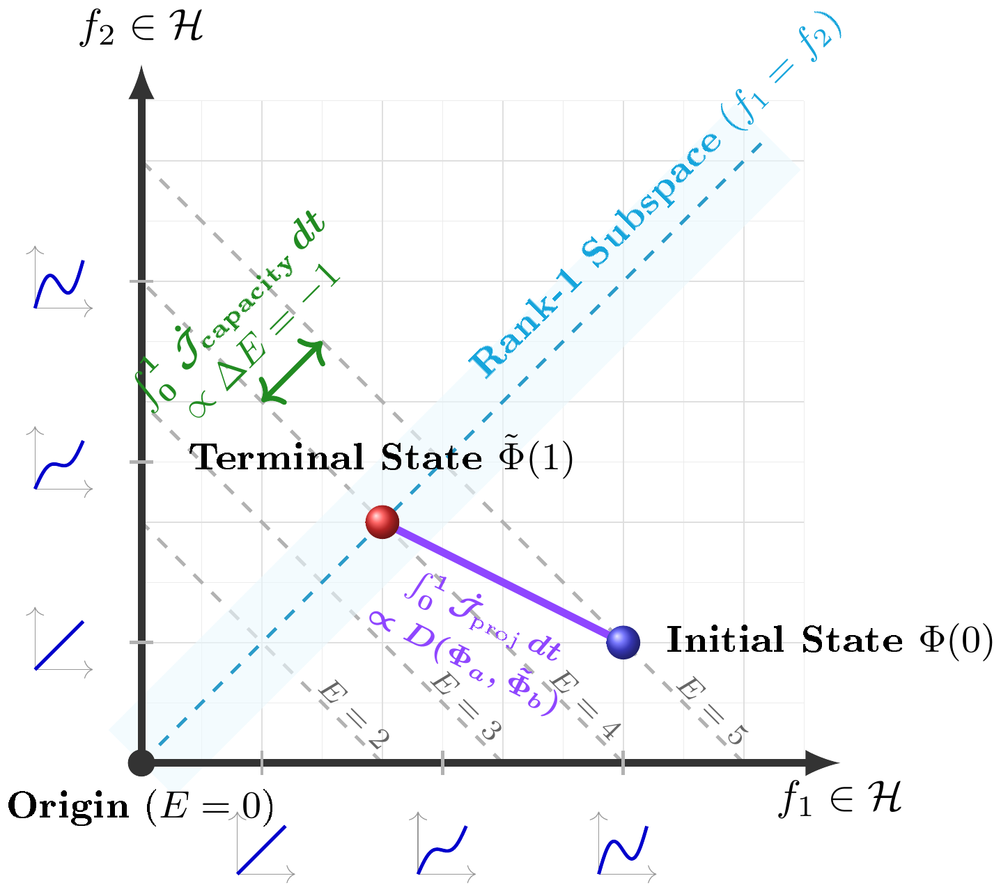
Despite the conceptual clarity of these transitions, their discrete nature (where the architecture hops from state $\Phi_a$ to $\Phi_b$ via pruning or merging) presents a significant barrier to mathematical analysis. To bridge the gap between abstract analysis and algorithmic execution, we proceed in two steps. First, we perform a continuous relaxation: instead of an instantaneous jump, we define a continuous deformation $\Phi(t)$ over $t \in [0, 1]$, interpolating between $\Phi(0) = \Phi_a$ and a pre-deletion target $\Phi(1) = \tilde{\Phi}_b$ (Figure 2). This allows us to use differential equations to express the infinitesimal cost of shrinking a layer's capacity. Second, to compute the total transition cost, we integrate this differential cost with respect to $t$. Our objective is to resolve this integral into an expression that depends only on the physically realizable endpoints ($\Phi_a$ and $\tilde{\Phi}_b$), bypassing the need to evaluate fictitious intermediate states along the continuous path. However, since this integral generally lacks a closed-form solution, and numerical evaluation incurs computationally prohibitive runtime overhead, we instead derive a closed-form upper bound on the analytically intractable integral.

Layer Capacity. To develop a layer cost $\mathcal{J}$, we first extend the single-neuron capacity, $|f_i|$, to define a layer capacity $E(\Phi)$ for state $\Phi$, where $E(f_1)=|f_1|$. A natural requirement is that $E(\Phi)$ remains invariant to arbitrary neuron partitioning. Assuming $E(\Phi)$ is a symmetric, separable, and homogeneous functional of individual capacities, this condition uniquely determines $E(\Phi) = \sum_{k=1}^N \lVert f_k\rVert_{\mathcal{H}}$ (by Lemma 1). For some intuition, suppose that $E(\Phi) = \left(\sum \lVert f_k\rVert_{\mathcal{H}}^p\right)^{1/p}$. Partitioning a neuron $f_0$ into $M$ fractions $f_0/M$ yields $M^{(1-p)/p} \lVert f_0\rVert_\mathcal{H}$. Capacity invariance for any $M$ requires $(1-p)/p = 0$, yielding $p=1$.

Axiomatic Cost Formulation. To ensure a well-posed definition of $\mathcal{J}$, we introduce the following natural axioms: 1. Magnitude Neutrality: $\mathcal{J}$ must be scale invariant: $\forall k > 0 , ;, \mathcal{J}(k, \Phi_a, k, \Phi_b) = \mathcal{J}(\Phi_a, \Phi_b)$. 2. Connectivity Preservation: $\mathcal{J}$ must establish an asymptotic barrier preventing layer extinction: $\lim_{E(\Phi_b) \rightarrow 0^+} \mathcal{J} = \infty$. 3. Infinitesimal Capacity Dependence: $\mathcal{J}$ must be additive along continuous paths and be driven by the reduction in layer capacity: $\mathcal{J}(\Phi_a, \Phi_b) = \int_{0}^{1} -\xi(\Phi(t)) \dot{E}(t) dt$, where $\dot{E}(t) \triangleq dE(\Phi(t))/dt$ and $\xi(\Phi(t)) > 0$ is a state-dependent density function. While Axioms 1 and 2 define boundaries of the theory, Axiom 3 acts as an idealized analytical tool modeling a continuous capacity drain $\dot{E}(t) < 0$. This allows us to deduce the fundamental shape of the cost function. Under these premises, we can prove (By Theorem 2) that $\mathcal{J}$ must obey $\mathcal{J}{\text{capacity}}(\Phi_a, \Phi_b) = \int{0}^{1} -c(\Phi(t)) \frac{\dot{E}(t)}{E(\Phi(t))} dt$, where $\dot{E}(t) < 0$ (due to capacity reduction) and $c(\Phi(t)) > 0$ is a scale-invariant factor (i.e., $c(k \Phi) = c(\Phi)$ for any $\Phi \in \mathcal{H}^N$ and $k > 0$).

Piecewise Constant $c(\Phi(.))$. To bridge continuous theory with discrete execution, we restrict $c(\Phi)$ to remain constant along any discrete state transition $\Phi_a \rightarrow \Phi_b$, e.g. $c(\Phi(t)) = c(\Phi_a)$ for $t \in [0, 1]$. This allows us to factor $c(\Phi)$ out of the integral for both $\mathcal{J}{\text{capacity}}$ and all subsequently derived cost functionals; for $\mathcal{J}{\text{capacity}}$, this directly yields the analytical solution $\mathcal{J}{\text{capacity}} = c(\Phi_a) \ln(\frac{E_a}{E_b})$. Upon reaching the terminal state, physically removing extinguished neurons causes $c(\Phi(t))$ to snap to a new value $c(\Phi_b)$. Consequently, $c(\Phi(t))$ acts as a globally piecewise constant function that remains locally constant during any integration step. While $\mathcal{J}{\text{capacity}}$ is not yet the final objective used in our optimizer, confirming that it satisfies Axioms 1 and 2 ensures we are on track, while its derivation via integration inherently satisfies the idealized capacity dependence assumption.

6.2 Bounding the Projection Cost

While $\dot{\mathcal{J}}(t)$ is driven by the relative capacity reduction $-\dot{E}/E$, our framework needs to minimize projection error[^6] (Section 5). We bridge the two by calibrating along an orthogonal trajectory where $ds = -dE$ translates the abstract capacity loss $-\dot{E}$ into a geometric speed $\dot{s}$. Here $s(t) = \int_{0}^{t} \lVert\dot{\Phi}(\tau)\rVert_{\mathcal{H}^N} d\tau$ is the arc-length swept by $\Phi(t)$ through the space $\mathcal{H}^N$. Because $\mathcal{H}^N$ is isotropic, this substitution generalizes to any arbitrary deformation path, yielding $\dot{\mathcal{J}}_{\text{proj}}(t) = c(\Phi(t)) \frac{\dot{s}(t)}{E(\Phi(t))}$ Equation (45). This substitution shifts $\mathcal{J}$ from pure capacity loss to any distance traversed, meaning the strict $\dot{E}(t) < 0$ assumption from the idealized model is no longer required along the physical path.

[^6]: Transitioning from $\mathcal{J}{\text{capacity}}$ to $\mathcal{J}{\text{proj}}$ ensures sensitivity to feature alignment. For instance, merging two orthogonal neurons introduces a severe subspace projection error while $\mathcal{J}{\text{capacity}}$ evaluates this catastrophic alignment loss identically to a merge between two collinear (hence redundant) neurons due to their equivalent linear capacity reductions. Shifting to $\mathcal{J}{\text{proj}}$ reorients the optimization objective from macroscopic reduction to minimizing distortion within the network's internal mapping.

The compression algorithm executes discrete leaps (e.g., snapping neurons $f_i$ and $f_j$ to a shared parent $f_p$). Evaluating the cost of this transition conceptually requires integrating $\dot{\mathcal{J}}{\text{proj}} = c \cdot \dot{s} / E$ over the jump path. However, because runtime integration is computationally prohibitive, we seek a fast, closed-form proxy. Since underestimating this integral risks destructive jumps (e.g., removing orthogonal features) and breaching layer depletion barriers before the continuous cost can diverge, we derive a closed-form upper bound to enforce cautious greedy optimization. We construct this bound by exploiting the inverse relationship between $\dot{\mathcal{J}}{\text{proj}}$ and $E$ in $\dot{\mathcal{J}}_{\text{proj}} = c \cdot \dot{s} / E$.

For any arbitrary deformation path connecting $\Phi_a$ to $\Phi_b$, we can establish an upper bound on the integral cost by replacing the dynamic capacity $E(t)$ with a constant minimum, $E_{\min}$, allowing us to pull the denominator outside the integral. This yields a bounded fractional cost where the numerator is the path's total arc length, $\int_{0}^{1} \dot{s}(t) dt$. Because infinitely many curves in $\mathcal{H}^N$ connect the two states, this establishes a family of valid upper bounds. To tighten this proxy cost, we minimize the numerator by selecting the path with the shortest arc length: the straight-line trajectory in $\mathcal{H}^N$. This evaluates to the traversed Euclidean distance $D(\Phi_a, \tilde{\Phi}b) \triangleq \lVert\Phi_a - \tilde{\Phi}b\rVert{\mathcal{H}^N} = (\sum{k=1}^N \lVert f_k^{(a)} - \tilde{f}k^{(b)}\rVert{\mathcal{H}}^2)^\frac{1}{2}$.

Next, to complete this bound, we must safely approximate the denominator's minimum $E_{\min}$ along this chosen straight-line path. Because the straight-line geometric path acts as a secant across the space of functions (abandoning the strict $\dot{E}(t) < 0$ assumption), the capacity $E(t)$ can temporarily dip below the pre-deletion target $E(\tilde{\Phi}_b)$. To safely absorb this without breaking the integral bound, we introduce a safety buffer by evaluating the denominator at the true terminal state $E(\Phi_b)$. For highly correlated neuron pairs, $E(t) \geq E(\Phi_b)$ throughout the straight-line transition (Lemma 3).

Substituting the minimized numerator $D$ and evaluating the constant denominator as $E(\Phi_b)$ yields the final bound $\mathcal{J}_{\text{proj}}(\Phi_a, \Phi_b) \le c(\Phi_a) \frac{D(\Phi_a, \tilde{\Phi}b)}{E(\Phi_b)} \equiv \mathcal{J}{\text{bound}}(\Phi_a, \Phi_b)$ (see Theorem 4). Here, $\tilde{\Phi}_b \in \mathcal{H}^N$ is the pre-deletion target at $t=1$ (e.g., a duplicated parent $[f_p, f_p]$) but the $N$-dimensional structure remains intact. Conversely, $\Phi_b \in \mathcal{H}^{N-1}$ is the true terminal state: the layer after the extinguished neuron is dropped. This separation ensures no dimensional mismatch in the arguments of $D$, while the denominator only relies on the $(N-1)$-dimensional post-deletion capacity $E(\Phi_b)$.

Axiomatic Consistency of the Bounded Proxy.

While the continuous functional $\mathcal{J}{\text{capacity}}$ was derived from our foundational axioms, the subsequent derivation of $\mathcal{J}{\text{bound}}$ alters the underlying differential equation. Specifically, to bypass the expensive runtime integration, we introduced a surrogate curve and bounded the capacity denominator. Because these approximations manipulate the original differential equation, it is no longer guaranteed a priori that the resulting closed-form proxy inherits the axiomatic properties of its continuous predecessor. However, we can prove that $\mathcal{J}{\text{bound}}$ (and consequently $\mathcal{J}{\text{final}}$) still preserves the foundational axioms of Magnitude Neutrality and Connectivity Preservation (by Proposition 5). However, the Infinitesimal Capacity Dependence assumption acts primarily as an analytical tool rather than a fundamental necessity, and is intentionally relaxed. Specifically, $\mathcal{J}{\text{capacity}}$ relies on integration over a path characterized by a monotonic capacity drain $\dot{E}(t) < 0$. However, deriving the closed-form $\mathcal{J}{\text{bound}}$ abandons this path integration in favor of a straight-line approximation evaluated at endpoints. Because this straight-line projection cuts directly across $\mathcal{H}^N$, the intermediate capacity along the path may temporarily fluctuate, violating the assumption of monotonic decrease required by the original differential equation. Consequently, $\mathcal{J}_{\text{bound}}$ knowingly sacrifices the path-additivity required by the modeling assumption. This relaxation is necessary to translate abstract continuous theory into an efficient $\mathcal{O}(1)$ evaluation of discrete state transitions.

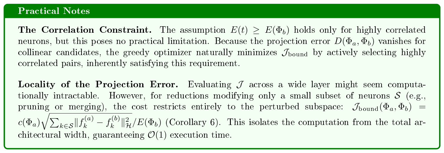
Choice of $c(\Phi)=N$. We previously specified $c(\Phi)$ to be piecewise constant; we now propose a more specific definition: setting $c(\Phi)=N$ for each continuous piece. This is to avoid unfair removal of critical diversity from wide layers by the global optimizer before addressing obvious redundancies in narrow bottlenecks, which may occur as capacity $E(\Phi)$ intrinsically scales with layer width. To mitigate this width bias, we normalize $\mathcal{J}$ using the average feature capacity[^7] $E(\Phi) / N$, which can be implemented by setting $c(\Phi)=N$. Substituting this $c(\Phi)$ into $\mathcal{J}{\text{bound}}$ yields the final cost $\mathcal{J}{\text{final}} , \triangleq, \frac{N \cdot D(\Phi_a, \tilde{\Phi}b)}{E(\Phi_b)}$. We can instantiate the pruning and merging costs as special cases of $\mathcal{J}{\text{final}}$.

[^7]: Consider a mean-field assumption where each active neuron contributes an average capacity $\bar{e}$. The incremental cost of pruning a single neuron evaluates to $\mathcal{J}{\text{prune}} \approx \frac{N \cdot \bar{e}}{N \cdot \bar{e}} = 1$. This normalization renders the penalty invariant to the instantaneous layer width. Without this dynamic coupling (e.g., if $c$ were anchored to $N{\text{initial}}$), the incremental cost would artificially explode as the live capacity shrinks, forcing an artificial uniformity that prevents the optimizer from fully extinguishing noisy, redundant blocks.

6.3 Final Pruning and Merging Costs

Pruning a neuron $f_i$ corresponds to projecting its rank-1 operator down to the null operator $\boldsymbol{0}$. Because the perturbed subspace only contains this single neuron $\mathcal{S} = {i}$ and its terminal state is $\boldsymbol{0}$, the projection error simplifies to $D = \sqrt{\lVert f_i - \boldsymbol{0}\rVert_{\mathcal{H}}^2} = \lVert f_i\rVert_{\mathcal{H}}$. By evaluating the terminal capacity as $E(\Phi_b) = E_a - \lVert f_i\rVert_{\mathcal{H}}$ we get $\mathcal{J}{\text{prune}} = \frac{N \cdot \lVert f_i\rVert{\mathcal{H}}}{E_a - \lVert f_i\rVert_{\mathcal{H}}}$.

Merging a neuron pair is slightly more involved. For neurons $i$ and $j$, their joint operator $[f_i, f_j]$ spans a rank-2 subspace in $\mathcal{H}$. Because $f_i$ and $f_j$ are vector-valued functions, their joint operator is matrix-valued, denoted as $\boldsymbol{W}{\text{joint}} \triangleq [f_i, f_j]$. Merging compresses this into a rank-1 approximation $\boldsymbol{W}{\text{joint}}'$. Classic unconstrained rank truncation (Eckart-Young-Mirsky) prescribes a rank-one basis $f_b$ and independent scaling factors $\alpha, \beta \in \mathbb{R}$ by solving $\min_{f_b \in \mathcal{H}, \alpha, \beta \in \mathbb{R}} \lVert \boldsymbol{W}{\text{joint}} - \boldsymbol{W}{\text{joint}}'\rVert^2_{\mathcal{H}}$, where $\boldsymbol{W}_{\text{joint}}' = [\alpha f_b, \beta f_b]$.

However, because a physical neuron must produce a single unified output, we must restrict the valid replacement pair to $\boldsymbol{W}{\text{joint}}' = [f_p, f_p]$. This enforces the constraint $\alpha = \beta = 1$, yielding the constrained objective $\min{f_p \in \mathcal{H}} \lVert \boldsymbol{W}{\text{joint}} - \boldsymbol{W}{\text{joint}}'\rVert^2_{\mathcal{H}}$ and rendering standard unconstrained projections inapplicable.

Deferring the derivation of the optimal parent $f_p$ to Section 7.1, we first establish the objective functional itself. Since the distance $D$ is the expected Frobenius projection error under the Hilbert-Schmidt norm, we expand it as follows:

$ D^2(\Phi_a, \Phi_b) = \lVert \boldsymbol{W}{\text{joint}} - \boldsymbol{W}{\text{joint}}'\rVert^2_{\mathcal{H}} = \mathbb{E}{\boldsymbol{x} \sim P{\mathcal{X}}} \left[\lVert \boldsymbol{W}{\text{joint}}(\boldsymbol{x}) - \boldsymbol{W}{\text{joint}}'(\boldsymbol{x})\rVert_F^2 \right] = \lVert f_i - f_p\rVert_{\mathcal{H}}^2 + \lVert f_j - f_p\rVert_{\mathcal{H}}^2 \nonumber , .\tag{6} $

The terminal capacity $E_b$ updates by swapping the eliminated children for the new parent: $E_b = E_a - \lVert f_i\rVert_{\mathcal{H}} - \lVert f_j\rVert_{\mathcal{H}} + \lVert f_p\rVert_{\mathcal{H}}$. Substituting $D$ and $E_b$ yields the final merging cost.

7. Generating the Parent Neuron

Section Summary: The process of generating a parent neuron begins by casting the merge of two existing neurons as an optimization problem in Hilbert space, where the parent function is decomposed into an adjustable magnitude and a unit direction that must itself be realizable by a neural-network layer. The inner optimization over direction is solved by maximizing alignment with the sum of the child neurons; after applying a kernel representation and a first-order approximation valid for common piecewise-linear activations such as ReLU, this alignment task reduces to a simple eigenvalue problem whose solution yields the optimal input weights. The resulting parent direction is then scaled by an outer magnitude search that balances reconstruction error against the increase in activation energy, producing a single neuron that can replace the two children with minimal impact on the network’s overall behavior.

7.1 The Parent Neuron in Hilbert Space

We determine the optimal parent neuron $f_p^*$ by minimizing $\mathcal{J}_{\text{merge}}(f_p)$ subject to $f_p\in \mathcal{N}$, where $\mathcal{N}$ denotes the space of realizable neurons:

$ \mathcal{N} \triangleq { f , |, f(\boldsymbol{x}) = \boldsymbol{w}{\text{out}} \Psi(\tilde{\boldsymbol{w}}{\text{in}} \cdot \tilde{\boldsymbol{x}}) } \subset \mathcal{H} , .\tag{8} $

Here $\tilde{\boldsymbol{x}} = [\boldsymbol{x}, 1]^T$ and $\tilde{\boldsymbol{w}}{\text{in}} = [\boldsymbol{w}{\text{in}}^{\text{eff}}, b]^T$ denote the augmented inputs and weights. Any non-zero function $f \in \mathcal{H}$ can be decomposed into a scalar magnitude $s > 0$ and a direction $\psi \in \mathcal{H}$, such that $f = s\psi$ and $|\psi|_{\mathcal{H}} = 1$. Applying this to the parent neuron $f_p$ allows us to reformulate the search for $f_p^*$ as the following nested optimization problem:

$ \min_{s \in \mathbb{R}^+} \min_{ \psi \in \mathcal{N}} \frac{\sqrt{|f_p - f_i|{\mathcal{H}}^2 + |f_p - f_j|{\mathcal{H}}^2}}{E_a - |f_i|{\mathcal{H}} - |f_j|{\mathcal{H}} + |f_p|{\mathcal{H}}} \qquad \text{s.t} \qquad f_p = s , \psi \quad, \quad \lVert\psi\rVert{\mathcal{H}} = 1 \quad, \quad s>0\tag{9} $

7.1.1 Optimal Direction

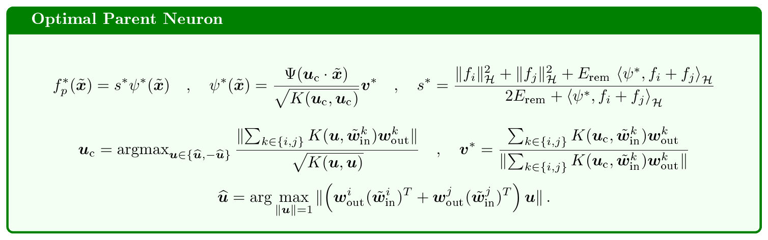
We first focus on the inner optimization problem of Equation (9). Expanding the squared numerator of the cost functional reveals that for a fixed magnitude $s > 0$, minimizing the cost in $\psi$ is equivalent to maximizing the alignment $\left\langle\psi, f_i + f_j\right\rangle_{\mathcal{H}}$ in $\psi$. To solve the latter, we enforce the realizability $\psi \in \mathcal{N}$ and unit-norm $\lVert\psi\rVert_{\mathcal{H}} = 1$ constraints by decoupling the input and output parameters, yielding the parametric form:

$ \psi = \frac{\Psi(\boldsymbol{u} \cdot \tilde{\boldsymbol{x}})}{\sqrt{K(\boldsymbol{u}, \boldsymbol{u})}} \boldsymbol{v} , .\tag{10} $

Substituting this parametric form into the unconstrained alignment objective and distributing the Hilbert inner product via the kernel identity isolates the output direction $\boldsymbol{v}$. By the Cauchy-Schwarz inequality, the optimal $\boldsymbol{v}^*$ must align with $\sum_{k \in {i, j}} K(\boldsymbol{u}^*, \tilde{\boldsymbol{w}}^k_{\text{in}}) \boldsymbol{w}^k_{\text{out}}$. Substituting this optimal $\boldsymbol{v}^*$ back into the objective simplifies the alignment inner product to the Euclidean norm of that sum, yielding the final objective for the optimal $\boldsymbol{u}^*$ (Theorem 7):

$ \boldsymbol{v}^* = \frac{\sum_{k \in {i, j}} K(\boldsymbol{u}^*, \tilde{\boldsymbol{w}}^k_{\text{in}}) \boldsymbol{w}^k_{\text{out}}}{\lVert\sum_{k \in {i, j}} K(\boldsymbol{u}^*, \tilde{\boldsymbol{w}}^k_{\text{in}}) \boldsymbol{w}^k_{\text{out}}\rVert} , , , , , \boldsymbol{u}^* = \operatorname{argmax}{\lVert \boldsymbol{u}\rVert=1} \frac{\lVert\sum{k \in {i, j}} K(\boldsymbol{u}, \tilde{\boldsymbol{w}}^k_{\text{in}}) \boldsymbol{w}^k_{\text{out}}\rVert}{\sqrt{K(\boldsymbol{u}, \boldsymbol{u})}} , \text{s.t.} , K(\boldsymbol{u}, \boldsymbol{u}) > 0\tag{11} $

The above optimization[^8] in $\boldsymbol{u}$ generally lacks a closed-form solution due to the non-linear nature of the kernel $K$. To maintain computational tractability, we introduce an approximation scheme that reduces the objective to an eigenvalue problem. Our approximation assumes that for any unit vector $\boldsymbol{x}$ and non-zero $\boldsymbol{y}$, the kernel factors as $K(\boldsymbol{x}, \boldsymbol{y}) = \lVert \boldsymbol{y}\rVert k\left(\left\langle \boldsymbol{x}, \frac{\boldsymbol{y}}{\lVert \boldsymbol{y}\rVert}\right\rangle \right)$ for some angular function $k : [-1, 1] \rightarrow \mathbb{R}$ bounded by $k(\rho) \leq 1$. Additionally, we require $k(1) = k'(1)$ and $k(1) > 0$. These conditions naturally hold for all PH-1 functions (piecewise linear with a single knot at the origin), e.g., ReLU, Leaky-ReLU; see Proposition 8 to Proposition 10. For highly correlated neuron pairings, the optimal parent direction $\boldsymbol{u}$ aligns closely with its children, pushing their cosine similarity $\rho \triangleq \left\langle \boldsymbol{u}, \frac{\tilde{\boldsymbol{w}}{\text{in}}}{\lVert\tilde{\boldsymbol{w}}{\text{in}}\rVert}\right\rangle$ toward $1$. Expanding $k(\rho)$ to first order around $\rho = 1$ and applying the $k(1) = k'(1)$ identity cancels the constant terms, yielding the linear approximation $k(\rho) \approx \rho k(1)$. While this degrades for unaligned vectors, the phase-check provided later in the section corrects anti-alignment by flipping the sign of $\boldsymbol{u}$, ensuring the optimization trajectory remains safely within this linear domain.

[^8]: By the PH-1 property of $\Psi$, the mapping $\boldsymbol{u} \mapsto K(\boldsymbol{u}, \boldsymbol{u})$ is homogeneous, implying that the objective is invariant to the transformation $\boldsymbol{u} \leftarrow c \boldsymbol{u}$ for any $c > 0$. We arbitrarily enforce $| \boldsymbol{u}|=1$ to keep the problem well-posed.

Applying the linear approximation to the numerator of the objective, and defining the constant matrix $\boldsymbol{A} \triangleq \boldsymbol{w}^i_{\text{out}} (\tilde{\boldsymbol{w}}^i_{\text{in}})^T + \boldsymbol{w}^j_{\text{out}} (\tilde{\boldsymbol{w}}^j_{\text{in}})^T$, the summation factors neatly: $ \sum_{k \in {i, j}} K(\boldsymbol{u}, \tilde{\boldsymbol{w}}^k_{\text{in}}) , \boldsymbol{w}^k_{\text{out}} \approx k(1) \boldsymbol{A} \boldsymbol{u}$. Conversely, the denominator requires no approximation; because $\lVert \boldsymbol{u}\rVert=1$, self-alignment $\rho=1$ evaluates to $K(\boldsymbol{u}, \boldsymbol{u}) = k(1)$. Substituting these into the original optimization problem gives: $ \widehat{\boldsymbol{u}} = \arg\max_{\boldsymbol{u}} \frac{\lVert k(1) \boldsymbol{A} \boldsymbol{u}\rVert}{\sqrt{k(1)}} \qquad\text{s.t.}\qquad \lVert \boldsymbol{u}\rVert=1 $. Because $k(1) > 0$, the scalars pull out. Dropping these constants and squaring the strictly non-negative objective simplifies the unconstrained problem to a standard quadratic form: $ \widehat{\boldsymbol{u}} = \arg\max_{\boldsymbol{u}} , \boldsymbol{u}^T \boldsymbol{A}^T \boldsymbol{A} \boldsymbol{u} \qquad\text{s.t.}\qquad \lVert \boldsymbol{u}\rVert=1$. The optimal direction $\widehat{\boldsymbol{u}}$ is simply the principal eigenvector of $\boldsymbol{A}^T \boldsymbol{A}$. While explicitly constructing this ambient matrix is computationally prohibitive, $\boldsymbol{A}$ is fundamentally rank-2. Restricting the eigendecomposition to this rank-2 subspace bypasses the ambient dimension entirely, yielding the principal eigenvector via a fast closed-form solution.

Determining the Sign of $\boldsymbol{u}$. For PH-1 activations, the kernel is sign-sensitive $K(\boldsymbol{u}, \tilde{\boldsymbol{w}}{\text{in}}) \neq K(-\boldsymbol{u}, \tilde{\boldsymbol{w}}{\text{in}})$. However, because our linearization approximation relies on the leading eigenvector $\widehat{\boldsymbol{u}}$ of $\boldsymbol{A}^T \boldsymbol{A}$, we only recover the solution up to a sign ambiguity. We resolve this by evaluating both candidate polarities $\pm\widehat{\boldsymbol{u}}$ in the exact, non-linearized objective Equation (11):

$ \boldsymbol{u}{\text{correct}} = \operatorname{argmax}{\boldsymbol{u} \in {\widehat{\boldsymbol{u}}, -\widehat{\boldsymbol{u}}}} \frac{\left\lVert\sum_{k \in {i, j}} K(\boldsymbol{u}, \tilde{\boldsymbol{w}}^k_{\text{in}}) \boldsymbol{w}^k_{\text{out}}\right\rVert}{\sqrt{K(\boldsymbol{u}, \boldsymbol{u})}} , .\tag{12} $

7.1.2 Optimal Scale

Recall from Equation (10) that the unit-norm direction $\psi \in \mathcal{N}$ is parameterized by unit vectors $\boldsymbol{u}$ and $\boldsymbol{v}$ as $\psi = \frac{\Psi(\boldsymbol{u} \cdot \tilde{\boldsymbol{x}})}{\sqrt{K(\boldsymbol{u}, \boldsymbol{u})}} \boldsymbol{v}$. Substituting $f = s\psi$ into the merging cost Equation 9 and defining constants $a \triangleq |f_i|{\mathcal{H}}^2 + |f_j|{\mathcal{H}}^2$, $b \triangleq \left\langle\psi, f_i+f_j\right\rangle_{\mathcal{H}}$, and $E_{\text{rem}} \triangleq E_a - |f_i|{\mathcal{H}} - |f_j|{\mathcal{H}}$, minimizing the squared objective reduces to the 1D problem $s^* = \operatorname{argmin}{s > 0} \frac{2s^2 - 2bs + a}{(s+E{\text{rem}})^2}$. Setting the derivative with respect to $s$ to zero yields the unique minimizer $s^* = \frac{a + b E_{\text{rem}}}{2 E_{\text{rem}} + b}$. This solution is also stable. By definition, the residual capacity $E_{\text{rem}} \ge 0$, and the prior phase-check ensures the alignment in function space $b > 0$. Thus, the denominator is strictly positive, guaranteeing a unique global minimum in the positive domain (simplifying cleanly to $s^* = a/b$ in the event of a total layer collapse where $E_{\text{rem}}=0$). Once the optimal scale $s^*>0$ is determined, the parent neuron is fully characterized as shown below.

7.2 From Hilbert Space to Physical Parameters

This section bridges the abstract function space and the physical parameter space by mapping the mathematical operator derived in $\mathcal{H}$ back into physical parameters. This parameter recovery is only necessary for merging. For pruning, the projection target is simply the null operator $\boldsymbol{0}$, which leads to $f(\boldsymbol{x}) = 0$; this is trivially realized by zeroing out the neuron's incoming weights, outgoing weights, and BN parameters. However, deploying the parent neuron $f_p^* \in \mathcal{H}$ derived in Equation (13) requires determining the physical parameters (weights $\boldsymbol{w}^\text{raw}p, b_p, \boldsymbol{w}{p, \text{out}}$ and BN statistics $\beta_p, \gamma_p, \mu_p, \sigma_p$) that will configure the forward pass to reproduce its targeted non-zero activation profile.

7.2.1 Input/Output Scaling

To form a standard realizable neuron as described in Equation (8), we equate $f_p^*(\tilde{\boldsymbol{x}}) = \boldsymbol{w}{\text{out}}^* \Psi(\tilde{\boldsymbol{w}}{\text{in}}^* \cdot \tilde{\boldsymbol{x}})$ and then specify the parameters $\tilde{\boldsymbol{w}}^*_{\text{in}}$ and $\boldsymbol{w}{\text{out}}^*$. Because the PH-1 activation $\Psi$ exhibits scale symmetry, the amplitude $s^* / \sqrt{K(\boldsymbol{u}^*, \boldsymbol{u}^*)}$ can be factored into arbitrary input and output scales $\tilde{\boldsymbol{w}}{\text{in}}^* = s_\text{in} \boldsymbol{u}^*$ and $\boldsymbol{w}{\text{out}}^* = s\text{out} \boldsymbol{v}^*$, for any $s_\text{in}, s_\text{out} \geq 0$ satisfying $s_\text{in} s_\text{out} = s^* / \sqrt{K(\boldsymbol{u}^*, \boldsymbol{u}^*)}$. While any factorization yields the same mapping $\mathcal{X} \rightarrow \mathbb{R}^c$, amplitude distribution impacts fine-tuning dynamics. To preserve the original layer's balance, we define the subspace Frobenius ratio $R_F \triangleq \lVert \boldsymbol{W}{\text{in}}\rVert_F / \lVert \boldsymbol{W}{\text{out}}\rVert_F$, where $\boldsymbol{W}{\text{in}} = [\tilde{\boldsymbol{w}}^i{\text{in}} \mid \tilde{\boldsymbol{w}}^j_{\text{in}}]$ and $\boldsymbol{W}{\text{out}} = [\boldsymbol{w}^i{\text{out}} \mid \boldsymbol{w}^j_{\text{out}}]$. Constraining the parent neuron to this ratio requires $\lVert\tilde{\boldsymbol{w}}^*_{\text{in}}\rVert_2 / \lVert \boldsymbol{w}^*_{\text{out}}\rVert_2 = R_F$. Since $\boldsymbol{u}^*$ and $\boldsymbol{v}^*$ are unit vectors, $s_\text{in} / s_\text{out} = R_F$. This uniquely determines the scale factors, yielding the final parameters:

$ \tilde{\boldsymbol{w}}{\text{in}}^* = \sqrt{s^* R_F} \cdot K\text{self}^{-1/4}, \boldsymbol{u}^* \qquad, \qquad \boldsymbol{w}{\text{out}}^* = \sqrt{\frac{s^*}{R_F}} \cdot K\text{self}^{-1/4} , \boldsymbol{v}^* \qquad, \qquad K_\text{self} \triangleq K(\boldsymbol{u}^*, \boldsymbol{u}^*) , .\tag{16} $

7.2.2 Raw Input and BN Parameters

While the Hilbert space formulation operates entirely on the effective input parameters $\tilde{\boldsymbol{w}}{\text{in}} \triangleq (\boldsymbol{w}{\text{in}}^{\text{eff}}, b)$, realizing the physical network requires recovering the underlying physical parameters: $\boldsymbol{w}^\text{raw}, \beta, \gamma, \mu, $ and $\sigma$. Since the parent direction $\widehat{\boldsymbol{u}}$ lies within the 2D subspace spanned by the augmented children, there exist projection coefficients $c_1$ and $c_2$ that produce the effective parameters:

$ \boldsymbol{w}{p, \text{in}}^{\text{eff}} = c_1 \boldsymbol{w}{\text{in}, i}^{\text{eff}} + c_2 \boldsymbol{w}_{\text{in}, j}^{\text{eff}} \quad \text{and} \quad b_p = c_1 b_i + c_2 b_j , .\tag{17} $

By mapping these coefficients through the pre-activation distributions of the children, we can deduce the required BN statistics for the parent neuron. Because the physical BN equations form an under-constrained system, we resolve the ambiguity by anchoring the variance such that $\sigma_p^2 = \max(0, \gamma_p^2 - \epsilon)$. As rigorously derived in Appendix D, this anchoring yields a closed-form recovery of all physical parameters. For the active regime $\gamma_p^2 \ge \epsilon$, these evaluate to:

$ \boldsymbol{w}{\text{in}, p}^{\text{raw}} = \boldsymbol{w}{\text{in}, p}^{\text{eff}} \qquad, \qquad \mu_p = c_1 \beta_i + c_2 \beta_j - b_p\tag{18} $

$ \beta_p = c_1 \beta_i + c_2 \beta_j \qquad, \qquad \sigma_p = \gamma_p = \sqrt{c_1^2 \gamma_i^2 + c_2^2 \gamma_j^2 + 2 c_1 c_2 |\gamma_i| |\gamma_j| \hat{\rho}_{ij}} , .\tag{19} $

where $\hat{\rho}_{ij}$ is from Equation (4). Note that $\sigma_p \approx \gamma_p$ is an approximation that assumes the numerical stability constant $\epsilon$ is negligible. The exact boundary-safe formulation $\sigma_p^2 = \max(0, \gamma_p^2 - \epsilon)$ and the edge case for inactive features $\gamma_p^2 < \epsilon$ are deferred to Appendix B.5. Furthermore, Appendix D provides the full step-by-step derivation, along with a proof demonstrating that the physical forward pass acts as a self-correcting mechanism that ensures the network's mapping remains invariant to the sign of the recovered scale $\gamma_p$.

8. Block Eviction

Section Summary: This section introduces block eviction as a macro-level pruning step for residual blocks in networks like ResNet-50. It forces the block’s internal pathway to zero, collapsing the block into a pure identity mapping that passes the input forward unchanged. The method extends earlier granular compression costs into a single unified formula that safely accounts for the skip connection, avoiding the bias shifts and wasted computation that arise when standard pruning leaves the block’s final layer intact.

This section expands the granular compression cost $\mathcal{J}_{\text{bound}}$ established in Section 6 to a new macro-level operation: block eviction. Focusing on residual blocks in architectures like ResNet-50, we extend the previously developed continuous integral to evaluate block eviction alongside granular operations within a single, unified mathematical framework.

Consider the canonical residual block, which processes an input representation $X$ (capitalized to distinguish it from the flattened vector $\boldsymbol{x}$) through a three-stage mapping pathway $F(X)$. This pathway sequentially applies weight parameters $W_1$, $W_2$, and $W_3$, and the result is added to a skip connection to yield the final pre-activation $Y = X + F(X)$. We define Block Eviction as forcing $F(X) \to \boldsymbol{0}$, and thus collapsing the block into a pure identity mapping $Y = X$ (see Figure 3).

8.1 Motivation

A dedicated macro-level operation is required because standard granular pruning cannot remove the block's final layer $W_3$. The output dimensionality of $F(X)$ must match the skip connection $X$ for element-wise addition. Consequently, granular compression can only deplete the internal layers $W_1, W_2$, which leaves the output channels of $W_3$ locked at their ambient size. Leaving a residual pathway active under these conditions creates two issues:

• Model Generalization: When $W_1$ and $W_2$ are heavily depleted, the pathway functionally reduces to injecting an uncalibrated BN effective bias $B_{\text{eff}}$ into the skip connection $Y = X + B_{\text{eff}}$. This shifts downstream feature maps out of their calibrated domain, often causing catastrophic ReLU clipping and irreversible information loss when going from $Y$ to $Z$.
• Execution Efficiency: Retaining the massive $W_3$ parameter tensor simply to process a negligible subspace violates the core objective of compression.

Block eviction resolves both issues by projecting the pathway $F(X)$ to the null operator. By yielding a pure identity mapping $Y = X$, we avoid uncalibrated bias injection and leverage the fact that residual architectures are inherently designed to be robust to identity mappings (e.g., standard $\gamma=0$ initialization practices) [87, 88]. Full mathematical details of this degradation are provided in Appendix F.

8.2 The Unified Macro Cost $\mathcal{J}_{\text{evict}}$

To evaluate this macro-operation within our framework, we must expand our definition of layer state. To see why, observe that Axiom 2 imposes an infinite cost penalty on projecting an entire layer to zero to prevent disconnecting the network graph. However, this penalty creates an artificial barrier here, as the parallel identity mapping preserves overall connectivity of the block and keeps it alive. To account for this skip pathway, we formulate a macroscopic state $\Omega^{(l)} \triangleq (\Phi^{(l)}, \mathcal{I})$ that couples the targeted internal layer $\Phi^{(l)}$ with the ambient skip connection $\mathcal{I}$.

The skip connection provides a parallel survival capacity $E_{\text{identity}}$ that keeps the mathematical projection stable. As rigorously derived in Appendix F, integrating the continuous capacity cost over this macro-state and applying a linear upper bound to safely govern massive discrete architectural leaps yields a closed-form distortion criterion. For a standard residual bottleneck comprising two internal convolution layers $l \in {1, 2}$, the total macroscopic distortion is the linear sum of their independent projection bounds:

$ \mathcal{J}{\text{evict}} = \sum{l=1}^{2} \mathcal{J}{\text{layer}}(\Omega_a^{(l)}, \Omega_b^{(l)}) = \sum{l=1}^{2} N_{\text{active}}^{(l)} \left(\frac{E_{\text{active}}^{(l)}}{E_{\text{identity}}} \right) , .\tag{20} $

Here, $N_{\text{active}}^{(l)}$ and $E_{\text{active}}^{(l)}$ represent the active operator count and surviving capacity of internal layer $l$, respectively. The parallel survival capacity evaluates to the expected RMS energy of the identity operators conditioned by the preceding BN layer: $E_{\text{identity}} = \sum_{k=1}^{d_{\text{amb}}} \sqrt{\gamma_k^2 + \beta_k^2}$.

9. Balancing Compression and Distortion

Section Summary: The section explains that pure distortion measures are insufficient for compression because stronger reductions in model size inherently increase error. To balance the two, the authors frame progressive compression as a planning task that selects a sequence of pruning, merging, or eviction steps to meet a fixed parameter budget while minimizing cumulative distortion. They relax the resulting hard combinatorial problem with a receding-horizon greedy heuristic that repeatedly picks the single operation offering the lowest distortion per parameter saved, then re-evaluates after each actual change.

All cost functionals discussed thus far ($\mathcal{J}{\text{prune}}$ and $\mathcal{J}{\text{merge}}$ for granular reductions, and $\mathcal{J}_{\text{evict}}$ for block evictions) measure the projection error incurred when transitioning from a given state to a reduced state. However, rate-distortion theory establishes that distortion alone cannot fully characterize a lossy compression scheme: lower signal distortion requires a higher bit count, while stronger compression inevitably increases distortion. To balance these competing objectives, we aim to minimize total distortion under a fixed bit count budget.

Progressive compression is therefore formulated as a trajectory planning problem within the action space. The goal is to craft a sequence of compression operations that yields a final model satisfying the allowable bit budget while minimizing the total accumulated distortion along the trajectory. Solving this represents a highly complex planning problem due to two primary challenges:

1. Dynamic State Dependency: The cost of an action changes continuously as the model transitions between states. For example, pruning a single neuron shrinks the layer's residual capacity, which instantaneously alters the cost $\mathcal{J}$ of subsequent operations, such as pruning another neuron or evicting an entire block. Consequently, the mathematical cost landscape is constantly shifting.
2. Mutually Exclusive Actions: The action space contains complex combinatorial dependencies. If the optimizer merges Neuron A with Neuron B, independent actions like "Prune A" or "Merge A with C" become permanently invalid.

For computational tractability, we must relax these constraints. At each iteration, we temporarily assume all currently admissible operations will remain valid for future iterations, ignoring their mutually exclusive nature. While this generates a complete theoretical action sequence, executing the full trajectory would introduce compounding errors in both state transitions and capacity counts. Instead, we adopt a receding-horizon strategy [89, 90]: we compute the optimal sequence, but execute only the immediate next action. Then we physically update the network and then re-evaluate all admissible functions from scratch. This single-step execution acts as an inherent auto-correction mechanism that ensures adherence to constraints over each short-term step.

Formally, let $\mathcal{A} = {1, 2, \dots, K}$ denote the set of all admissible compression operations at the current encoding iteration, encompassing all feasible granular and macro operations. Each action $k$ incurs a distortion penalty $\mathcal{J}_k$ and releases $\Delta P_k$ parameters (see Appendix B.2 for details on computing $\Delta P$). Assuming a standard fixed-precision representation (e.g., 32-bit floating-point), bit reduction is proportional to parameter reduction. This direct scaling allows us to express the allowable budget directly in terms of the parameter footprint. We frame this optimization as:

$ (a_1^*, \cdot s, a_K^*) = \arg\min_{a_1, \cdot s, a_K} \sum_{k=1}^K a_k \mathcal{J}k \qquad\text{s.t.}\qquad \sum{k=1}^K a_k \Delta P_k \geq P_0 - P_{\text{budget}} \quad, \quad \forall k , ;, a_k \in {0, 1} , .\tag{22} $

where $P_0$ is the initial parameter count and $P_{\text{budget}}$ is the maximum allowable parameter footprint for the final model. This formulation is a discrete knapsack problem, which is well-known to be NP-Hard [91, 92]. We resolve this using a continuous relaxation heuristic, replacing the binary constraint $a_k \in {0, 1}$ with a continuous bound $0 \leq a_k \leq 1$. This transforms the objective into a continuous knapsack problem (a specific class of linear programming) that admits a highly efficient analytical solution. As established by Dantzig [93], the exact optimal solution is found greedily: candidates are sorted by their distortion rate (DR), defined as the cost-to-capacity ratio $\mathcal{J}_k / \Delta P_k$, and assigned $a_k = 1$ in ascending order until the budget constraint is saturated. Because our receding-horizon framework executes only the single next action, the problem reduces to selecting the operation with the minimal DR:

$ k^* = \arg\min_{k \in \mathcal{A}} \frac{\mathcal{J}_k}{\Delta P_k} , .\tag{23} $

While the receding-horizon strategy mitigates the dynamic dependency of $\mathcal{J}$, the continuous knapsack solver still requires $\Delta P$ to satisfy Dantzig's Axiom of Item Independence: the weight of one item cannot depend on the selection state of another. Particularly in our problem, evaluating operations using the dynamically shrinking live parameter footprint $\Delta P$ violates this axiom because adjacent layers share weight matrices; pruning a neuron physically shrinks the $\Delta P$ of its neighbors.

A naive optimization using this live $\Delta P$ triggers a failure mode: as a layer is compressed, the expected DR of neighboring structures artificially inflates. This repels the optimizer and may trap the architecture in a fragmented state that prevents the removal of contiguous blocks. Decoupling parameter yield from dynamic state via the static surrogate $\Delta P_k^{\text{init}}$ restores item independence and avoids this failure mode:

10. The Encoding Loop

Section Summary: The encoding loop compresses a neural network by repeatedly selecting and applying the single best pruning or merging step according to the lowest distortion-to-parameter ratio. It begins by precomputing and caching every neuron’s capacity along with all pairwise merge costs across layers. In each cycle the algorithm scans the entire network to locate the globally optimal action, executes it, then refreshes only the local values around the changed neurons so that subsequent scans remain efficient, continuing until the size target is met.

With the optimal action selection now formally defined, we execute progressive encoding as a greedy dynamical system. At a high level, the algorithm continuously identifies the optimal action $k^*$ offering the lowest DR $\mathcal{J}_k/\Delta P_k^{\text{init}}$, performs a localized recalculation exclusively for the modified structures (e.g., a newly generated parent neuron $f_p^*$) and their immediate neighbors, decrements the relevant dimension count, and repeats. Specifically, the process operates in the following three phases and terminates once the target physical parameter budget is reached or no admissible compression operations remain:

1. Initialization: Before compression begins, the algorithm precomputes and caches the individual capacities of all neurons, the pairwise geometric cross-capacities of all valid merging pairs, and the total initial capacity of every layer (establishing the starting value for $E_{\text{rem}}$).

2. The Greedy Scan: At each iteration, the algorithm scans all $L$ layers (each containing roughly $N$ active neurons) to find the single optimal compression action $k^*$ yielding the lowest DR $\mathcal{J}_k/\Delta P_k^{\text{init}}$. For pruning, evaluating every individual candidate across the network requires $\mathcal{O}(L \cdot N)$ operations. For merging, evaluating every valid pair requires checking $\frac{N(N-1)}{2}$ combinations per layer, leading to $\mathcal{O}(L \cdot N^2)$ operations. Because querying the cached $\mathcal{J}$ for each candidate takes $\mathcal{O}(1)$ time[^9], the total computational complexity to find the optimal action at any step is bounded by the pairwise merge evaluations at $\mathcal{O}(L \cdot N^2)$.

[^9]: As established in the practical notes of Section 6, the distortion cost $\mathcal{J}$ relies on local variables: the capacity of the targeted neurons and the remaining capacity of their specific layer. Because evaluating $\mathcal{J}$ does not require querying the global network state, calculating the DR of any individual prune, merge, or block eviction operation is $\mathcal{O}(1)$.

3. Localized Update: Once the globally optimal action is identified and executed, the network state must be synchronized. The algorithm decrements the layer's $E_{\text{rem}}$ by the capacity flux removed by the operation, and decrements the neuron count $N$. If the action was a merge, the algorithm also computes the capacity of the newly generated parent neuron $f_p^*$ and calculates the cross-capacities as well as optimal projection vectors) between this new parent and the $N-1$ surviving neighbors in its layer. These updated constants are injected into the cache, guaranteeing that the evaluation of $\mathcal{J}$ during subsequent greedy scans remains $\mathcal{O}(1)$. This limits the network state recalculation to an $\mathcal{O}(N)$ local update.

11. Proof-of-Concept Applications

Section Summary: HOPE supports two practical uses by leveraging its neuron-level capacity estimates. In model compression it progressively removes entire neurons to generate smaller networks that retain higher accuracy than magnitude-based pruning baselines on ImageNet-trained ResNet-50. In transfer learning the related DEFT method uses the same estimates to split a network into a protected core and an adaptable periphery, allowing efficient fine-tuning on new domains without overwriting prior knowledge.

11.1 Model Compression

Because its encoding is progressive, any intermediate iteration serves as a valid compressed model, providing users with flexible trade-offs between compression rate and fidelity. Taxonomically, HOPE is a structured method: it eliminates entire neurons rather than zeroing out individual weights. This provides greater practical utility than unstructured pruning, which generates randomly sparse matrices requiring specialized hardware to realize actual computational speedups. We compare HOPE against three structured baselines that eliminate neurons below specific magnitude thresholds: $L_1$-Norm Input Pruning [28] (scored by incoming weight $L_1$ norms); $L_1$-Norm Joint Pruning (scored by concatenated incoming and outgoing $L_1$ norms); and BN Scale Pruning [28] (using the BN scaling factor $\gamma$ as a proxy for importance).

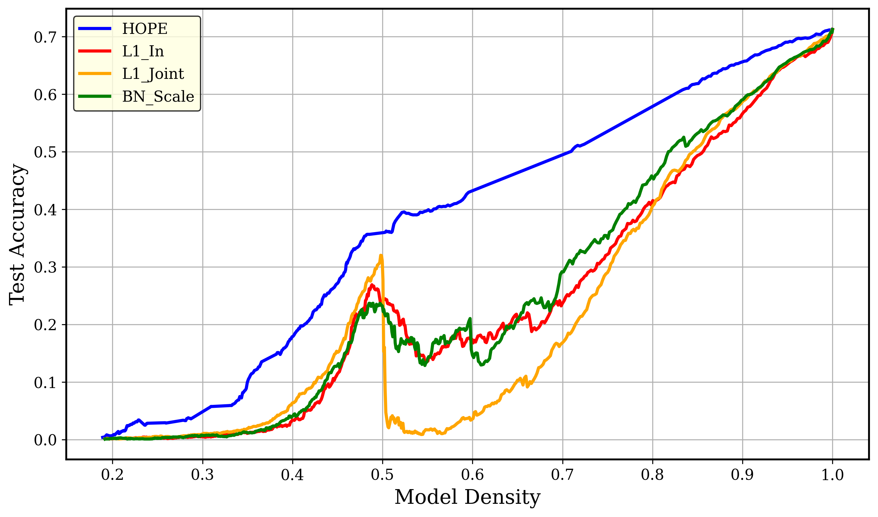
Our experiments investigated the relationship between test set accuracy and model density (defined as the ratio of active to initial neurons across the entire network). For our compression assessment, we utilized Keras' publicly available ResNet-50 model checkpoint that is pre-trained on ImageNet. As demonstrated in the plot, HOPE yields models with superior accuracy compared to the baselines.

11.2 Cross-Domain Transfer Learning

HOPE’s capacity evaluation can be used for resolving the stability-plasticity dilemma in transfer learning. By merging redundancies, we can partition the network into a protected core and a plastic periphery and leverage it for parameter-efficient transfer.

11.2.1 The Stability-Plasticity Dilemma and Current Bottlenecks

Intelligent systems face a fundamental challenge: adapting to new domains without erasing foundational knowledge, a trade-off known as the Stability-Plasticity dilemma [70]. Cognitive neuroscience models this via Complementary Learning Systems [73, 74], proposing that the brain insulates a stable, domain-specific core from a plastic periphery, as empirically supported by recent neuroimaging [94, 95, 96]. Specifically, the brain extracts generalizable schemata from noisy state transitions by applying low-dimensional regularization to its representational geometry [97].

During standard training, deep neural networks self-organize into a similar, albeit noisy and imperfect, dichotomy [98]. They develop a sparse, load-bearing core surrounded by low-capacity representational slack [19, 99]. Naively exploiting this emergent segregation by freezing the core fails; because layers remain entangled, peripheral updates shift activation flows, causing representational drift. Early solutions like PackNet [100] circumvented this using binary masks during inference, but these scale poorly and require a priori task identities.

Robust continual learning requires explicit interventions, rather than relying on noisy emergent segregation. During source training, regularization [26, 101] can amplify the segregation. During downstream adaptation, penalty-based methods like EWC [71], Synaptic Intelligence [72], and second-order pruning [17, 18, 30] prevent drift using locally convex Fisher Information Matrices (FIMs) or Hessians. However, relying on local approximations makes these algorithms brittle to large domain shifts. Conversely, orthogonal projection methods stop drift by restricting updates to the null-space of previous tasks [102, 76, 77, 103, 78, 79]. However, they remain computationally expensive due to the $\mathcal{O}(N^3)$ operations and source forward passes needed to compute covariance matrices.

11.2.2 DEFT

To address the above challenges, we introduce Dispersed Elastic Fine-Tuning (DEFT). Aligning with the Information Bottleneck principle [6], DEFT treats learning as the compression of irrelevant slack space via global Hilbert-Schmidt operators, bypassing local loss curvature and empirical data passes. Leveraging the HOPE framework, DEFT analytically computes each neuron's capacity in $\mathcal{O}(N)$ time to partition the network into a Universal Core and a Peripheral Slack. To prevent representational drift, DEFT severs weight projections from the slack to the core prior to transfer. This ensures the core remains frozen while the slack adapts, eliminating the need for inference-time masking or task identities.

DEFT governs parameter plasticity through a binary elasticity map $E \in {0, 1}$. While prior methods also regulate plasticity [104], their reliance on weight sensitivity leaves them vulnerable to the scaling symmetries that HOPE mitigates. We formalize this by evaluating the pruning cost assigned to each neuron $i$ upon its removal during HOPE's progressive encoding process:

$ \mathcal{J}{\text{prune}}^{(i)} = \frac{N^{(i)} \cdot |f_i|{\mathcal{H}}}{E_b^{(i)}}\tag{25} $

where $N^{(i)}$ and $E_b^{(i)} \triangleq E_a^{(i)} - \lVert f_i\rVert_{\mathcal{H}}$ denote the active neuron count and the remaining layer capacity, at the step neuron $i$ is pruned. To establish a global freezing threshold, we collect the set of all such costs across the entire encoding process, and filter out extinction artifacts resulting from near-zero capacities:

$ \mathcal{C} = \left{ \mathcal{J}_{\text{prune}}^{(i)} ;\middle|; E_b^{(i)} > \epsilon \right}\tag{26} $

Given a target percentile hyperparameter $P \in [0, 100]$, we compute the threshold $J_P = \text{Percentile}(\mathcal{C}, P)$ and the supremum $J_{\sup} = \max(\mathcal{C})$. For numerical stability against edge capacity regimes, the final locking threshold $J_{\text{lock}}$ is defined:

$ J_{\text{lock}} = \begin{cases} J_P & \text{if } J_P \ge \epsilon \ J_{\sup} & \text{if } J_P < \epsilon \text{ and } J_{\sup} \ge \epsilon \ 1 & \text{otherwise} \end{cases}\tag{27} $

The elasticity of neuron $i$ is formulated as:

$ E_i = \begin{cases} 1 & \text{if } \mathcal{J}{\text{prune}}^{(i)} < J{\text{lock}} \ 0 & \text{if } \mathcal{J}{\text{prune}}^{(i)} \ge J{\text{lock}} \end{cases}\tag{28} $

Under this formulation, high capacity neurons essential to the source architecture $\mathcal{J}{\text{prune}}^{(i)} \ge J{\text{lock}}$ are frozen by $E_i=0$, whereas low-capacity slack neurons are granted high plasticity via $E_i=1$.

Dynamic Resolution of Redundancy: Deep networks frequently fragment a single feature across multiple correlated neurons. If we freeze the network based on a static capacity threshold, we incorrectly lock up this redundant volume and deprive the target task of parameter space. As illustrated in Figure 4(a), DEFT resolves this by compressing these redundant features into a single rank-1 parent neuron. This consolidates the foundational source knowledge while releasing the freed child neurons into the plastic slack $E_i=1$. By transforming redundant copies into uncommitted parameter space, DEFT actively generates capacity for the target task.

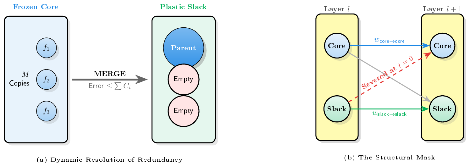
Consistency at Initialization (The Structural Mask): To prevent target-driven updates of the plastic slack from corrupting the frozen core, DEFT applies a structural mask at initialization (Figure 4 b). It severs all connections pointing from upstream plastic neurons to downstream frozen core neurons. For a weight tensor connecting an upstream layer (with elasticities $\boldsymbol{E}{\text{in}}$) to a downstream layer (with elasticities $\boldsymbol{E}{\text{out}}$), the mask $\boldsymbol{M}$ enforces:

$ M_{j, k} = \begin{cases} 0 & \text{if } E_{\text{in}, k} > 0 \text{ and } E_{\text{out}, j} = 0 \ 1 & \text{otherwise} \end{cases}\tag{29} $

The initial weights for the target task are thus constrained to $\boldsymbol{W}0 = \boldsymbol{M} \odot \boldsymbol{W}{\text{source}}$.

Theoretical Guarantees: We prove in Appendix H that these mechanisms protect the source representation through a layer-to-layer bounding framework. First, the Static Initialization Shock Bound establishes that severing the slack-to-core connections introduces a static error strictly bounded by $\mathcal{O}(\tau)$. Second, Dynamic Decoupling guarantees the core experiences zero dynamic interference during target fine-tuning. Because the cross-connections are severed at initialization and their weights are frozen from updating, any drifting signal from the learning slack subset is multiplied by zero, nullifying it before it can penetrate the core. Combined with the bounded projection errors of the merging operation, this framework ensures the cumulative degradation of the source task cannot compound exponentially, remaining anchored to an algorithmically verifiable constant.

Gradient Scaling: During optimization, the target gradients are element-wise scaled by the downstream neuron's elasticity $\boldsymbol{E}_{\text{out}}$ (uniformly broadcast across the input channels):

$ \boldsymbol{g}t = \boldsymbol{E}{\text{out}} \odot \nabla_{\boldsymbol{W}} \mathcal{L}_{\text{target}}(\boldsymbol{W}_t)\tag{30} $

where $\boldsymbol{g}_t$ represents the effective gradient passed to the optimizer state[^10], e.g., SGD with momentum.

[^10]: Scaling the gradient before the optimizer step prevents velocity drift for frozen parameters.

11.2.3 Experimental Setup

To evaluate the stability-plasticity tradeoff, we rank methods using the H-Score commonly used in continual learning [105, 106, 107]. H-Score, defined as the harmonic mean of source retention and target accuracy, heavily penalizes poor performance in either domain. This ensures a high score is achieved only when a model excels on both tasks.

We evaluate models pre-trained on multi-class classification tasks derived from the CIFAR-100 dataset [108]. Each source task is constructed by randomly sampling 4 superclasses, which yields 20 fine-grained categories (5 per superclass). Building the source task around dense semantic clusters rather than sampling 20 arbitrary classes forces the network to learn hierarchical features to distinguish closely related concepts. We then transfer these specialized models to the full 10-class digit classification task in the SVHN dataset (street-level house numbers) [109].

As summarized in Table 1, we benchmark DEFT against the following baseline methods:

• Standard Full FT: The entire pre-trained backbone is unfrozen, allowing the optimizer to alter representations across all layers. While maximizing target plasticity, it is highly susceptible to catastrophic forgetting.
• Head-Only FT (Standard FT): Representing the opposite extreme (linear probing), the pre-trained backbone is completely frozen, acting as a static feature extractor. Only the final linear classification head is optimized.
• PEFT (BN-Tuning): Operating on the premise that spatial feature extraction logic should remain invariant [110], this method applies a binary gradient mask: core convolutional and dense kernels are frozen, while plasticity is isolated entirely to the affine BN parameters (scale $\gamma$ and shift $\beta$) and the newly initialized classification head.
• EWC (Elastic Weight Consolidation): Allows all parameters to update but applies a quadratic penalty constraining parameters deemed critical to the source task [71]. To accurately lock foundational features, the empirical diagonal Fisher Information Matrix (FIM) is computed strictly over the source training dataset. See Appendix G for the per-example FIM derivation and integration protocol.

Table 1 provides a conceptual summary of these methodologies. Full details regarding network architecture, hyperparameter optimization, and reproducibility protocols are provided in Appendix G.

: Table 1: Comparative Summary of Transfer Learning Methodologies

Property	Full FT	Head-Only	PEFT	EWC	DEFT (Ours)
Updates Backbone Features	✓	-	-	✓	✓
Mitigates Catastrophic Forgetting	-	✓	✓	✓	✓
Parameter-Specific Modulation	-	-	-	✓	✓
Source Data Independence	✓	✓	✓	-	✓
Structure & Redundancy Aware	-	-	-	-	✓

11.2.4 Results and Discussion

The final test set evaluations across $4$ independent cross-domain trials ($20$ discrete CIFAR-100 $\to$ SVHN scenarios) are presented in Table 2. While Standard Full FT achieves the highest target performance $94.09%$ by freely overwriting network weights, it completely destroys the source representation, crashing source retention to a baseline low of $7.52%$. Conversely, Head-Only FT best preserves source knowledge, but its $36.11%$ target accuracy highlights the severe domain gap; pre-trained features are insufficient to separate SVHN digits linearly. EWC behaves remarkably similarly to Full FT: it learns the target domain ($93.94%$) but fails to significantly arrest catastrophic forgetting ($6.74%$). DEFT successfully bridges this stability-plasticity gap. By routing target gradients into elastic neurons characterized by their low capacity, DEFT captures nearly all the plasticity of Standard Full FT ($94.09%$ vs. $89.79%$). Simultaneously, by masking the core foundational features, it halts catastrophic forgetting, retaining $52.14%$ of the source accuracy. Computing the harmonic mean of the two accuracy values leads to the H-Score of method, in which DEFT significantly outperform all the baselines.

\begin{tabular}{@lccc@}
\toprule
\textbf{Method} & \textbf{Target Acc (SVHN)} & \textbf{Source Retention (CIFAR)} & \textbf{H-Score} \\
\midrule
\textbf{DEFT} (Ours) & $89.79 \pm 0.84$ & $52.14 \pm 5.29$ & $\mathbf{65.82 \pm 3.96}$ \\
\textbf{Head-Only} & $36.11 \pm 2.79$ & $63.13 \pm 4.62$ & $45.79 \pm 2.05$ \\
\textbf{Full FT} & $94.09 \pm 0.28$ & $7.52 \pm 1.63$ & $13.88 \pm 2.84$ \\
\textbf{EWC} & $93.94 \pm 0.22$ & $6.74 \pm 1.74$ & $12.54 \pm 2.99$ \\
\textbf{PEFT} & $81.91 \pm 0.49$ & $5.44 \pm 0.98$ & $10.18 \pm 1.63$ \\
\bottomrule
\end{tabular}

12. Acknowledgment

We thank Juno Kim, Vaishnavh Nagarajan, Atish Agarwala, Spencer Frei, Lisa Schut, Alan Malek, Gil shamir, and Bruno Mlodozeniec of Google DeepMind for their helpful comments and discussions.

Appendix

Section Summary: The appendix introduces Hilbert spaces as a rigorous setting for neural network compression in the HOPE framework, where operations such as pruning or merging are viewed as projections that require a well-defined space, a way to measure closeness through inner products, and completeness to ensure solutions exist. It defines an inner product via expected alignment of neuron functions over a data distribution, which satisfies the necessary mathematical properties, and embeds these functions into the L2 space to keep all optimizations inside a complete environment. The discussion further splits each neuron into continuous and discrete parts via tensor products so that the geometric calculations remain computationally practical.

A. Hilbert Spaces

This section provides a quick introduction to Hilbert spaces, focusing on the concepts of inner products, completeness, and total sets. We bridge abstract functional analysis with the specific architectural choices of the HOPE framework, demonstrating how the $L_2$ embedding of neural functions creates a unique and complete geometric environment for optimization over network structures.

A.1 Introduction: Why a Hilbert Space?

We treat compression operations like pruning and merging as projections. When we replace two neurons with one, we are attempting to find a single element that "represents" a multi-dimensional subspace. To perform this operation rigorously, we need three things:

1. A Space that contains all possible neural identities.
2. A Metric (Inner Product) to measure "closeness" and "alignment."
3. Completeness to ensure that our optimizations actually have solutions.

A Hilbert space $\mathcal{H}$ provides these three pillars.

A.2 The Inner Product: The Ruler of Geometry

The defining feature of a Hilbert space is the inner product. While a vector space only lets us add and scale elements, an inner product space lets us talk about angles and lengths.

########## {caption="Definition: Inner Product Axioms"}

An inner product on a vector space $V$ over $\mathbb{R}$ is a mapping $\left\langle\cdot, \cdot\right\rangle : V \times V \to \mathbb{R}$ satisfying for all $f, g, h \in V$ and $a \in \mathbb{R}$:

• Symmetry: $\left\langle f, g\right\rangle = \left\langle g, f\right\rangle$.
• Linearity: $\left\langle af + g, h\right\rangle = a\left\langle f, h\right\rangle + \left\langle g, h\right\rangle$.
• Positive Definiteness: $\left\langle f, f\right\rangle \geq 0$, and $\left\langle f, f\right\rangle = 0 \iff f = 0$.

A.2.1 Connection to HOPE: The Expectation Metric

In the HOPE framework, we operate on functions $f: \mathcal{X} \to \mathbb{R}^c$. We define our inner product relative to a surrogate distribution $P_{\mathcal{X}}$:

$ \left\langle f_i, f_j\right\rangle_{\mathcal{H}} \triangleq \mathbb{E}{\boldsymbol{x} \sim P{\mathcal{X}}} \left[f_i(\boldsymbol{x})^T f_j(\boldsymbol{x}) \right]\tag{31} $

########## {caption="Proposition: Validity of the HOPE Metric"}

The functional defined in Equation (31) satisfies the inner product axioms.

Proof: Linearity and symmetry follow directly from the linearity of the expectation operator $\mathbb{E}$ and the symmetry of the Euclidean dot product. Positive definiteness is guaranteed because $\left\langle f, f\right\rangle = \mathbb{E}[\left\lVert f(\boldsymbol{x})\right\rVert^2] \geq 0$. The definiteness $\left\langle f, f\right\rangle=0 \implies f=0$ is satisfied in the $L_2$ sense (i.e., $f$ is zero "almost everywhere").

A.3 The Ambient Space: $L_2(\mathcal{X}, P_{\mathcal{X}})$

A Hilbert space is more than just an inner product space; it must be complete. In finite dimensions (like $\mathbb{R}^n$), every inner product space is complete. In function spaces, this is not true.

########## {caption="Definition: Completeness"}

A space is complete if every Cauchy sequence ${f_n}$ (a sequence where elements get arbitrarily close to each other) converges to an element $f$ that is also inside the space.

If we worked only with continuous functions, the space would not be complete. For example, a sequence of continuous functions can converge to a step function (which is discontinuous). This would be a disaster for compression, as our "best parent" might not even exist in our space.

A.3.1 The $L_2$ Embedding

To avoid this, HOPE embeds neurons into $L_2(\mathcal{X}, P_{\mathcal{X}})$, the space of square-integrable functions.

• Energy Bound: Every function in $\mathcal{H}$ has finite energy: $\mathbb{E}[\left\lVert f\right\rVert^2] < \infty$.
• Closure: By definition, $L_2$ is complete. Every optimization we perform (minimizing the cost functional of compression operations) is guaranteed to have a valid result within the ambient space.

A.4 The Tensor Product: Splitting Continuous and Discrete Spaces

While we defined our ambient space as vector-valued functions $\mathcal{H} = L_2(\mathcal{X}, P_{\mathcal{X}}; \mathbb{R}^c)$, computing the inner product directly in this monolithic space obscures the internal structure of a neural network. HOPE simplifies this by utilizing a tensor product space.

A neuron's operation naturally splits into two phases:

1. The Continuous Input Landscape: The effective input weights (which absorb BN statistics) and the activation function create a continuous scalar landscape $g_i(\boldsymbol{x}) = \Psi((\boldsymbol{w}{\text{in}, i}^{\text{eff}})^T \boldsymbol{x} + b_i)$. We embed this function into a scalar Hilbert space $\mathcal{H}{\text{in}} \triangleq L_2(\mathcal{X}, P_{\mathcal{X}}; \mathbb{R})$.
2. The Discrete Output: This scalar activation is broadcast to the next layer along a finite-dimensional output weight vector $\boldsymbol{w}{\text{out}, i}$. We define this output space as $\mathcal{H}{\text{out}} \triangleq \mathbb{R}^c$.

By taking the tensor product of these two spaces, we construct the full ambient space mapping: $\mathcal{H} \cong \mathcal{H}{\text{in}} \otimes \mathcal{H}{\text{out}}$. Under this formulation, each individual neuron is modeled as a rank-1 Hilbert-Schmidt operator, represented by the outer product of its input function and output vector:

$ f_i \triangleq g_i \otimes \boldsymbol{w}_{\text{out}, i}\tag{32} $

A.4.1 Factoring the Metric

This tensor structure is what makes HOPE computationally tractable. The inner product of two rank-1 tensors elegantly factors into the product of their individual space inner products:

$ \left\langle f_i, f_j\right\rangle_{\mathcal{H}} = \left\langle g_i \otimes \boldsymbol{w}{\text{out}, i}, g_j \otimes \boldsymbol{w}{\text{out}, j}\right\rangle_{\mathcal{H}} = \left\langle g_i, g_j\right\rangle_{\mathcal{H}{\text{in}}} \cdot \left\langle \boldsymbol{w}{\text{out}, i}, \boldsymbol{w}{\text{out}, j}\right\rangle{\mathcal{H}_{\text{out}}}\tag{33} $

Because $\left\langle g_i, g_j\right\rangle_{\mathcal{H}{\text{in}}}$ is the expected alignment of their non-linear activations over the distribution $P{\mathcal{X}}$, we define this as the kernel $K(i, j)$. This allows us to separate the continuous-functional evaluation from the discrete parameters, reducing the full Hilbert space inner product to:

$ \left\langle f_i, f_j\right\rangle_{\mathcal{H}} = K(i, j) \cdot \left\langle \boldsymbol{w}{\text{out}, i}, \boldsymbol{w}{\text{out}, j}\right\rangle_{\mathbb{R}^c}\tag{34} $

A.5 Uniqueness and the Total Set Property

One might ask: "We defined the inner product for any functions $f, g$. But in HOPE, we only ever calculate it for single ReLU neurons. Is that enough to define the whole space?"

This is the most critical part of the theory.

########## {caption="Definition: Total Set"}

A set $S \subset \mathcal{H}$ is a total set if the set of all finite linear combinations of elements in $S$ is dense in $\mathcal{H}$.

If $S$ is total, then knowing the inner product for every pair in $S$ uniquely determines the inner product for the entire Hilbert space.

A.5.1 The Universal Approximation Theorem

In the context of HOPE, our "dictionary" of functions is the set of single neurons $\mathcal{N}$:

$ \mathcal{N} = { f(\boldsymbol{x}) = \boldsymbol{w}{out} \Psi(\tilde{\boldsymbol{w}}{\text{in}} \cdot \tilde{\boldsymbol{x}}) }\tag{35} $

########## {caption="Theorem: HOPE Uniqueness"}

The set $\mathcal{N}$ is a total set in $L_2(\mathcal{X}, P_{\mathcal{X}})$.

Discussion: By the Universal Approximation Theorem, linear combinations of ReLU neurons can approximate any square-integrable function to arbitrary precision. In the language of Hilbert spaces, this means $span(\mathcal{N})$ is dense in $\mathcal{H}$.

Because $\mathcal{N}$ is total, the definition of the function correlation kernel $K(i, j) = \mathbb{E}[\Psi(y_i)\Psi(y_j)]$ is sufficient to uniquely characterize the metric of the entire ambient space. We do not need a "separate" definition for the inner product of sums of neurons; it is uniquely forced upon the space by the behavior of the single neurons.

A.6 Neuron Synthesis by Projection

Finally, we see why this matters. The generation process relies on finding an Optimal Subspace Projection. When we want to merge neurons $i$ and $j$, their joint contribution $[f_i, f_j]$ spans a 2-dimensional tensor subspace. Because a physical parent neuron must produce a single unified output, it is modeled as a constrained rank-1 approximation $[f_p, f_p]$.

Rather than a simple orthogonal projection of a sum, HOPE finds the optimal parent $f_p^*$ by minimizing the expected Frobenius projection error under the Hilbert-Schmidt norm, scaled by the remaining capacity of the layer:

$ f_p^* = \operatorname{argmin}{f_p \in \mathcal{N}} \frac{\sqrt{\left\lVert f_i - f_p\right\rVert{\mathcal{H}}^2 + \left\lVert f_j - f_p\right\rVert_{\mathcal{H}}^2}}{E_a - \left\lVert f_i\right\rVert_{\mathcal{H}} - \left\lVert f_j\right\rVert_{\mathcal{H}} + \left\lVert f_p\right\rVert_{\mathcal{H}}}\tag{36} $

In a Hilbert space, the numerator translates to a rigorous geometric projection distance. Without the Hilbert space structure (inner products and completeness), the concepts of "closest operator" and "functional alignment" would have no meaning.

A.7 Summary

A summary of the key concepts and their utility in HOPE are provided in Table 3.

::: {caption="Table 3: Mapping of Abstract Hilbert Concepts to the HOPE Framework."}

:::

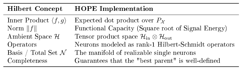
B. Implementation Notes

B.1 Adaptation for Convolutional Layers

Our formalism extends to convolutional networks by defining a "neuron" as a filter in layer $A$ producing feature map $i$. The joint parameter vector $\boldsymbol{w}_i = [\boldsymbol{w}_n^\top, \boldsymbol{w}_c^\top]^\top$ is constructed by vectorizing the filter's respective input and output kernels. The input space vector $\boldsymbol{w}n$ encapsulates the filter's local receptive field. Assuming layer $A$ possesses a weight tensor $\boldsymbol{K}A \in \mathbb{R}^{h_A \times w_A \times C{\text{in}} \times C{\text{out}}}$, the vector $\boldsymbol{w}_n$ corresponding to filter $i$ is the flattened spatial slice $\boldsymbol{K}A[:, :, :, i] \in \mathbb{R}^n$, where $n = h_A \times w_A \times C{\text{in}}$. Conversely, the output space vector $\boldsymbol{w}_c$ captures the filter's downstream influence on the subsequent layer $B$. Because the activation map of filter $i$ acts as the $i$-th input channel to layer $B$, $\boldsymbol{w}_c$ is formed by extracting and flattening the corresponding slice of the downstream tensor $\boldsymbol{K}B[:, :, i, :] \in \mathbb{R}^c$, where $c = h_B \times w_B \times C{\text{out}, B}$.

To allow the surrogate distribution to serve as a location-invariant prior without requiring intractable coordinate-specific covariance modeling, we assume spatial stationarity (ergodicity) across the feature map and construct it using the globally averaged BN variance $\sigma_i^2$. While boundary zero-padding breaks local stationarity, the high-dimensional spatial aggregation of modern BN buffers absorbs these edge-effects into a into a single global average.

B.2 Deriving the Parameter Footprint $\Delta P$

As established in Section 9, the parameter footprint $\Delta P$ quantifies the number of physical parameters removed by a compression action. To preserve Dantzig's Axiom of Item Independence, this criterion uses a static surrogate, $\Delta P^{\text{init}}$, evaluated on the initial network state and decoupled from the dynamically changing network. For any operation, the footprint tracks the total removed parameters:

$ \Delta P^{\text{init}} = |W_{\text{in}}|0 + |W{\text{out}}|0 + |\theta{\text{aux}}|_0\tag{37} $

where $W_{\text{in}}$, $W_{\text{out}}$, and $\boldsymbol{\theta}_{\text{aux}}$ denote the input weights, output weights, and auxiliary parameters (e.g., BN parameters) respectively, and $|\cdot|_0$ counts the number of non-zero elements.

B.2.1 Granular Operations

For pruning or merging, $\Delta P^{\text{init}}$ comprises the incoming weights, outgoing weights, and BN parameters of a single target neuron or filter. For example:

• Transformer MLP: Removing a neuron in an MLP with a $d_{\text{model}} \rightarrow 4d_{\text{model}}$ expansion yields $\Delta P^{\text{init}} = 2d_{\text{model}} + 1$.
• Convolutional Networks: For a filter with spatial dimensions $H \times W$, the footprint scales with the receptive field and projective kernel: $\Delta P^{\text{init}} = H \cdot W \cdot C_{\text{in}} + C_{\text{out}} + 4$, where $4$ accounts for the BN parameters $\gamma, \beta, \mu, \sigma^2$.

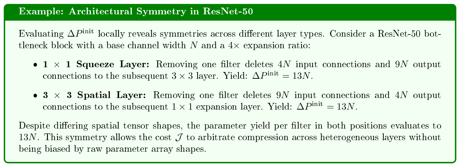
B.2.2 Macro Operations: Block Eviction

Unlike granular operations that yield incremental savings, block eviction removes entire layers simultaneously. For a residual block with internal convolutional layers $W_1$ and $W_2$, and a terminal expansion layer $W_3$, the static parameter yield expands to:

$ \Delta P_{\text{evict}}^{\text{init}} = |W_1|_0 + |W_2|0 + |\theta{\text{aux}}|_0\tag{38} $

where $|W_1|0$ and $|W_2|0$ denote the parameters of the internal layers, and $|\theta{\text{aux}}|0$ counts the BN parameters $\mu, \sigma^2, \gamma, \beta$ across the entire block, including those of $W_3$. Note that the weight matrix $W_3 \in \mathbb{R}^{d{\text{amb}} \times d{\text{bottleneck}}}$ is not explicitly included in this sum. Because removing a filter in $W_2$ removes its corresponding outgoing connections in $W_3$, the memory footprint of $W_3$ is naturally accounted for when evaluating $W_2$. Explicitly adding the ambient dimensions $|W_3|0 = d{\text{amb}} \times d_{\text{bottleneck}}$ would count the same parameters twice within a single macro action. This intra-action double-counting would inflate the parameter footprint of block eviction and artificially lower its Distortion Rate (DR), giving it an unfair advantage over granular operations.

B.3 Cross-Action Overlap and Uniform Scaling

While we avoid counting parameters twice within a single action (as seen with $W_3$), evaluating the entire decision space using a static footprint $\Delta P^{\text{init}}$ introduces an overlap between different competing actions. Let $i$ and $j$ be targeted neurons in adjacent layers $l$ and $l+1$. To preserve Dantzig's Axiom of Item Independence, an action targeting layer $l$ must not alter the state variables used to evaluate layer $l+1$. Consequently, their shared weight $W^{(l)}{j, i}$ is counted independently in both evaluations: $W^{(l)}{j, i} \in \Delta P_i^{\text{init}}$ and $W^{(l)}_{j, i} \in \Delta P_j^{\text{init}}$.

For any sequence of actions $\mathcal{S}$, this cross-action overlap overestimates the true number of parameters recovered $\sum_{k \in \mathcal{S}} \Delta P_k^{\text{init}} > \Delta P_{\mathcal{S}}^{\text{live}}$. This overestimation artificially lowers the computed DR compared to the live network state:

$ \text{DR}_k = \frac{\mathcal{J}_k}{\Delta P_k^{\text{init}}} < \frac{\mathcal{J}_k}{\Delta P_k^{\text{live}}}\tag{39} $

To correct this approximation without violating item independence, HOPE relies on uniform scaling. Because this cross-action overlap applies systematically across the entire action space $\mathcal{A}$ (all granular and macro candidates interact with their neighbors), it acts as a uniform scaling factor $\alpha \ge 1$ such that $\Delta P_k^{\text{init}} \approx \alpha \Delta P_k^{\text{live}}$.

Because the distortion cost $\mathcal{J}$ is evaluated independently of the parameter counts, and $\alpha$ applies uniformly, the relative ordering of the distortion rates is preserved:

$ \frac{\mathcal{J}_a}{\Delta P_a^{\text{init}}} < \frac{\mathcal{J}_b}{\Delta P_b^{\text{init}}} \iff \frac{\mathcal{J}_a}{\Delta P_a^{\text{live}}} < \frac{\mathcal{J}_b}{\Delta P_b^{\text{live}}}\tag{40} $

Since the greedy continuous knapsack solver selects $\arg\min_{k \in \mathcal{A}} \text{DR}_k$, this uniform scaling ensures that the theoretical fairness of the optimal action selection remains intact.

B.4 Computational Complexity and the Decoupled Cache

Evaluating the transition cost $\mathcal{J}$ efficiently poses a computational challenge because it is inversely coupled to the monotonically decreasing layer capacity $E_{\text{rem}}$. In a layer with $N$ neurons, recomputing the non-linear weight-space geometry (e.g., Rank-2 Singular Value Decompositions) for all $\mathcal{O}(N^2)$ candidate pairs every time $E_{\text{rem}}$ decreases requires $\mathcal{O}(N^3)$ execution time.

Conversely, caching $\mathcal{J}$ values in a standard priority queue via submodular approximations (e.g., Minoux's Lazy Update) leads to stale estimations. Because the transition cost goes to $\infty$ as capacity approaches $0$, small capacity reductions cause the true costs to spike. A delayed queue would underestimate these costs and cause the optimizer to select sub-optimal actions and potentially collapse the layer. We resolve this bottleneck using an $\mathcal{O}(1)$ Decoupled Cache.

Decoupling.

The computationally expensive optimal projections $\boldsymbol{u}^*, \boldsymbol{v}^*$ and the cost components ($a = |f_i|{\mathcal{H}}^2 + |f_j|{\mathcal{H}}^2$ and $b = \left\langle\psi^*, f_i+f_j\right\rangle_{\mathcal{H}}$, derived in Section 7.1) depend only on weights and static BN parameters associated with that layer. Since our method does not rely on any cross-layer criterion (such as Fisher Information), we guarantee that $\boldsymbol{u}^*, \boldsymbol{v}^*, a, b$ remain independent of both the downstream architecture and the dynamic capacity $E_{\text{rem}}$.

The only variable dependent on $E_{\text{rem}}$ is the optimal scalar magnitude $s^*$. At initialization, the framework computes $\boldsymbol{u}^*$ and $\boldsymbol{v}^*$ to evaluate and cache only the scalar constants $a$ and $b$. To prevent $\mathcal{O}(N^2)$ memory exhaustion, the high-dimensional vectors $\boldsymbol{u}^*, \boldsymbol{v}^*$ are then discarded. During the greedy search, evaluating the cost of any action requires querying the cached constants and the live remaining capacity $E_{\text{rem}} = \max(E_a - |f_i|{\mathcal{H}} - |f_j|{\mathcal{H}}, \epsilon)$ to compute $s^*$ and $\mathcal{J}$ analytically in $\mathcal{O}(1)$ time:

$ s^* = \frac{a + b E_{\text{rem}}}{2 E_{\text{rem}} + b}\tag{41} $

Index Determinism and JIT Generation.

We sort the active neurons to evaluate undirected pairs only where $i < j$. By enforcing this index determinism, the algorithm guarantees a 100% cache hit rate and makes it viable to abandon priority queues entirely. At every step, the algorithm executes an $\mathcal{O}(1)$ global scan over all remaining pairs using the live layer capacity, maintaining mathematically perfect freshness. Once the global minimum is selected, the framework executes a Just-In-Time (JIT) generation, re-evaluating the fast Rank-2 SVD only for the single winning pair ($\sim 1$ ms) to retrieve its $\boldsymbol{u}^*, \boldsymbol{v}^*$ for physical deployment.

Computing the BN Variance.

Deploying the JIT-generated parent requires setting its BN variance $\gamma_p^2$. Under the surrogate distribution $P_{\mathcal{X}}$, $\gamma_p^2$ depends only on the warped correlation $\hat{\rho}{ij}$. A naive approach might substitute the simple correlation of the raw weights $\rho{\text{raw}}$ into the variance equation. However, this incorrectly mixes parameter-space metrics with signal-space statistics. Doing so produces incorrect BN moving averages, which miscalibrates the network during the forward pass. The framework avoids this by computing the physical variance using $\hat{\rho}_{ij}$ directly retrieved from the cache. This ensures the deployed parameters maintain the correct statistical behavior without requiring empirical forward passes.

B.5 Numerical Stability and BN Parameters

Section 7.2.2 derives the mapping from the parent neuron's effective parameters ($\boldsymbol{w}{\text{in}, p}^{\text{eff}}$ and $b_p$) to its physical network variables: the raw input weights $\boldsymbol{w}{\text{in}, p}^{\text{raw}}$ and the BN parameters $\gamma_p, \beta_p, \mu_p, \sigma_p^2$. A naive assignment of these physical variables alters the pre-activation signal and breaks the critical equivalence $y_p = (\boldsymbol{w}_{\text{in}, p}^{\text{eff}})^T \boldsymbol{x} + b_p$. This mismatch miscalibrates the network and immediately degrades accuracy on the first forward pass.

To prevent this, HOPE enforces the exact analytical mapping. However, deploying these formulas in practice requires safely handling numerical bounds, such as preventing negative variance $\sigma_p^2 < 0$ and avoiding NaN in the BN denominator $\sqrt{\sigma_p^2 + \epsilon}$. This section details how to resolve these numerical edge cases and ensure the deployed model remains mathematically well-defined and numerically stable.

B.5.1 The $\epsilon$ Boundary Regime and Variance Clamping

To resolve the under-constrained BN system, the framework fixes the physical variance as $\sigma_p^2 = \max(0, \gamma_p^2 - \epsilon)$, where $\epsilon$ is a small stability constant (e.g., $10^{-5}$). For active features $\gamma_p^2 \ge \epsilon$, this evaluates smoothly. This allows the denominator of the BN transformation to simplify to $|\gamma_p|$.

However, as the progressive encoder shrinks the network, the derived parent variance $\gamma_p^2$ may occasionally fall below the numerical floor $\epsilon$. Without the $\max(0, \cdot)$ operator, enforcing $\sigma_p^2 = \gamma_p^2 - \epsilon$ would result in a negative variance, which causes NaN during inference. The clamping operator safely bounds the physical variance at $\sigma_p^2 = 0$.

When $\sigma_p^2$ is clamped to $0$, the BN denominator $\sqrt{\sigma_p^2 + \epsilon}$ evaluates to $\sqrt{\epsilon}$. Consequently, the scale factor becomes $\gamma_p / \sqrt{\epsilon}$. Substituting this into the effective bias equation yields:

$ b_p = \beta_p - \frac{\gamma_p}{\sqrt{\epsilon}} \mu_p \quad \implies \quad \mu_p = \frac{\sqrt{\epsilon}}{\gamma_p} (\beta_p - b_p)\tag{42} $

As the parent neuron's scale $\gamma_p$ approaches $0$, dividing by $\gamma_p$ causes $\mu_p \rightarrow \infty$. To prevent this, the framework bypasses this calculation for inactive features and sets $\boldsymbol{w}_{\text{in}, p}^{\text{raw}} = \boldsymbol{0}$.

B.5.2 Running Variance Offset During Fine-Tuning

Setting the initial BN running variance to $\sigma_p^2 = \gamma_p^2 - \epsilon$ ensures the network's output is perfectly preserved during inference. However, when the model resumes training for fine-tuning, the actual batch variance computed during the forward pass evaluates to $\sigma_{\text{batch}}^2 = \gamma_p^2$. This introduces a minor mismatch between the empirical batch variance and the stored running variance:

$ \sigma_{\text{batch}}^2 - \sigma_p^2 = \gamma_p^2 - (\gamma_p^2 - \epsilon) = \epsilon\tag{43} $

Because this discrepancy evaluates to the numerical constant $\epsilon$ (typically $10^{-5}$), its impact is negligible. Standard optimizers (e.g., Adam, AdamW) seamlessly absorb this $\mathcal{O}(\epsilon)$ offset during the initial training steps without destabilizing the network or degrading performance.

C. Main Paper Proofs

C.1 Layer Transition Costs

For convenience, we first recall the axioms of the cost $\mathcal{J}$ from the main paper.

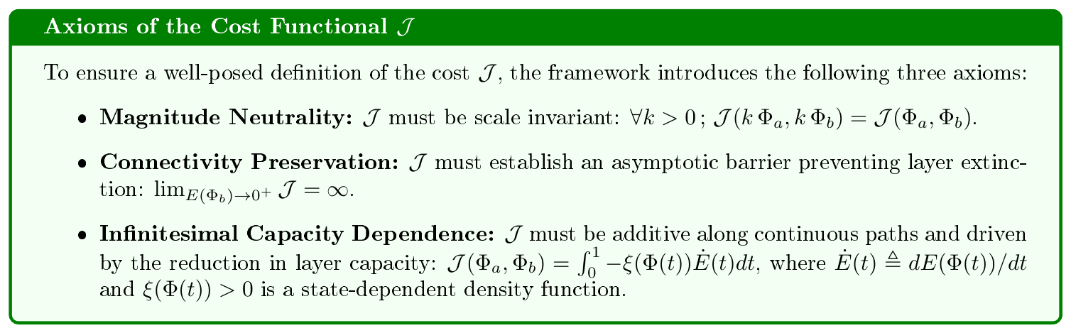
########## {caption="Lemma 1: Uniqueness of the $L_1$ Capacity"}

Let $\Phi = (f_1, \dots, f_N) \in \mathcal{H}^N$ denote a layer state. Assume the capacity functional $E: \bigcup_{N=1}^\infty \mathcal{H}^N \to \mathbb{R}_{\ge 0}$ satisfies:

1. Identity: $\forall f \in \mathcal{H}, ; E((f)) = \left\lVert f\right\rVert_{\mathcal{H}}$.
2. Symmetry & Separability: $\exists , g: \mathbb{R}{\ge 0} \to \mathbb{R}$ (continuous and strictly monotonic) and a function $h$ such that $\forall \Phi \in \mathcal{H}^N, ; E(\Phi) = h\left(\sum{k=1}^N g(\left\lVert f_k\right\rVert_{\mathcal{H}}) \right)$.
3. Partition Invariance: $\forall f \in \mathcal{H}, , \forall N \in \mathbb{Z}{\ge 1}, ; E((f)) = E\big((\underbrace{f/N, \dots, f/N}{N \text{ times}})\big)$.

Then $E(\Phi) = \sum_{k=1}^N \left\lVert f_k\right\rVert_{\mathcal{H}}$.

Proof: For a single-neuron state $\Phi = (f)$, Conditions 1 and 2 imply:

$ E((f)) = h\big(g(\left\lVert f\right\rVert_{\mathcal{H}})\big) = \left\lVert f\right\rVert_{\mathcal{H}} \implies h \equiv g^{-1} \text{ on } \text{Im}(g) $

Thus, the functional simplifies to $E(\Phi) = g^{-1}\left(\sum_{k=1}^N g(\left\lVert f_k\right\rVert_{\mathcal{H}}) \right)$.

By Condition 3 and the positive homogeneity of the norm ($\left\lVert f/N\right\rVert_{\mathcal{H}} = \left\lVert f\right\rVert_{\mathcal{H}}/N$ for $N \ge 1$):

$ \left\lVert f\right\rVert_{\mathcal{H}} = E\big((\underbrace{f/N, \dots, f/N}{N \text{ times}})\big) = g^{-1}\left(\sum{k=1}^N g\left(\frac{\left\lVert f\right\rVert_{\mathcal{H}}}{N}\right) \right) = g^{-1}\left(N g\left(\frac{\left\lVert f\right\rVert_{\mathcal{H}}}{N}\right) \right) $

Applying $g$ to both sides and substituting $x \triangleq \left\lVert f\right\rVert_{\mathcal{H}} \ge 0$ yields:

$ g(x) = N g\left(\frac{x}{N}\right) \qquad \forall x \ge 0, ; \forall N \in \mathbb{Z}_{\ge 1} $

For $x=0$, $g(0) = N g(0) \implies g(0) = 0$. For any rational $q = M/N > 0$, substituting $y = x/N$ yields $g(My) = M g(y) = q N g(y) = q g(Ny)$, meaning $g(qx) = qg(x)$. Since $g$ is continuous, this linearity extends to all $x \in \mathbb{R}_{\ge 0}$, yielding $g(x) = cx$ for some constant $c$. Since $g$ is strictly monotonic, $c \neq 0$.

Substituting $g(x) = cx$ and $g^{-1}(y) = y/c$ into the expression for $E(\Phi)$ gives:

$ E(\Phi) = \frac{1}{c} \sum_{k=1}^N c \left\lVert f_k\right\rVert_{\mathcal{H}} = \sum_{k=1}^N \left\lVert f_k\right\rVert_{\mathcal{H}} $

########## {caption="Theorem 2: Integral Formulation of Scale-Invariant Cost"}

Under the Axioms of Magnitude Neutrality, Connectivity Preservation, and Infinitesimal Capacity Dependence, the transition cost along a continuous deformation path $\Phi: [0, 1] \rightarrow \mathcal{H}^N $ with boundary conditions $\Phi(0) = \Phi_a$ and $\Phi(1) = \Phi_b$, is determined as the integral:

$ \mathcal{J}(\Phi_a, \Phi_b) = \int_{0}^{1} -c(\Phi(t)) \frac{\dot{E}(t)}{E(\Phi(t))} dt[^11]\tag{44} $

where $E(\Phi(t))$ is the instantaneous capacity, $\dot{E}(t) < 0$ is the rate of capacity reduction, and $c(\Phi(t)) > 0$ is a scale-invariant factor.

Proof:

1. Differential Form: By the Infinitesimal Capacity Dependence axiom, the differential cost along a path is driven by capacity reduction:

$ \dot{\mathcal{J}}(t) = -\xi(\Phi(t)) \dot{E}(t) $

Since active capacity decreases during compression $\dot{E}(t) < 0$ and the cost rate must be positive $\dot{\mathcal{J}}(t) > 0$, we require $\xi(\Phi(t)) > 0$.

2. Magnitude Neutrality: For any scalar $k > 0$, Magnitude Neutrality requires $\mathcal{J}(k\Phi_a, k\Phi_b) = \mathcal{J}(\Phi_a, \Phi_b)$. By Lemma 1, capacity scales linearly $E(k\Phi) = kE(\Phi)$, so $\dot{E}(k\Phi(t)) = k\dot{E}(t)$. Integrating over the scaled path yields:

$ \int_{0}^{1} -\xi(k\Phi(t)) , k , \dot{E}(t) dt = \int_{0}^{1} -\xi(\Phi(t)) \dot{E}(t) dt $

Assuming continuous integrands, since this equality holds for any valid continuous path, the integrands must be identical pointwise:

$ k , \xi(k\Phi) \dot{E}(t) = \xi(\Phi) \dot{E}(t) \implies \xi(k\Phi) = k^{-1} \xi(\Phi) $

Thus, $\xi$ is a homogeneous function of degree $-1$.

3. Scale-Invariant Factor: Define $c(\Phi) \triangleq \xi(\Phi) E(\Phi)$. Scaling the state by $k$ yields:

$ c(k\Phi) = \xi(k\Phi) E(k\Phi) = (k^{-1} \xi(\Phi)) (k E(\Phi)) = c(\Phi) $

This shows $c(\Phi)$ is scale-invariant. Substituting $\xi(\Phi) = c(\Phi) / E(\Phi)$ back into the differential form gives the integral:

$ \mathcal{J}(\Phi_a, \Phi_b) = \int_{0}^{1} -c(\Phi(t)) \frac{\dot{E}(t)}{E(\Phi(t))} dt $

4. Connectivity Preservation: This axiom mandates an infinite cost barrier against layer extinction: $\lim_{E_b \to 0^+} \mathcal{J}(\Phi_a, \Phi_b) = \infty$, where $E_b = E(\Phi_b)$ and $E_a = E(\Phi_a)$. Applying the change of variables $dE = \dot{E}(t) dt$ and reversing the limits (which absorbs the negative sign since $E_b < E_a$ due to $\dot{E}(t)<0$) gives:

$ \mathcal{J}(\Phi_a, \Phi_b) = \int_{E_a}^{E_b} -c(\Phi) \frac{dE}{E} = \int_{E_b}^{E_a} c(\Phi) \frac{dE}{E} $

If $c(\Phi)$ is bounded below by a constant $c_{\min} > 0$ along the path to extinction:

$ \mathcal{J}(\Phi_a, \Phi_b) \ge \int_{E_b}^{E_a} c_{\min} \frac{dE}{E} = c_{\min} \big(\ln(E_a) - \ln(E_b) \big) $

Taking the limit as $E_b \to 0^+$ yields $\infty$, satisfying the axiom.

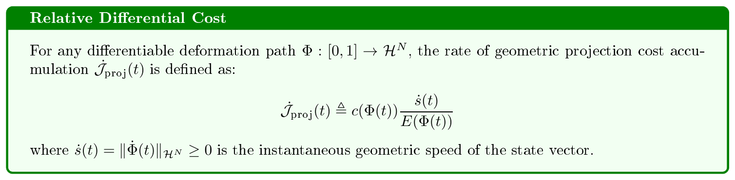
Derivation: The scalar capacity rate $\dot{E}(t)$ from Theorem 2 assigns zero penalty to geometric deformations (e.g., orthogonal rotations) where scalar capacity is conserved $\dot{E}(t) = 0$. To capture structural distortion, we calibrate the criterion along a localized orthogonal path.

Consider a compressive path where a single active neuron $f_k$ is scaled toward $\boldsymbol{0}$ by a decreasing scalar $\alpha(t) \in [0, 1]$ $\dot{\alpha}(t) < 0$, while all other neurons remain static. The capacity is $E(\Phi(t)) = \alpha(t) \left\lVert f_k\right\rVert_{\mathcal{H}} + \sum_{i \neq k} \left\lVert f_i\right\rVert_{\mathcal{H}}$, giving $\dot{E}(t) = \dot{\alpha}(t) \left\lVert f_k\right\rVert_{\mathcal{H}} < 0$.

The geometric speed $\dot{s}(t)$ is the norm of the state derivative vector. Since only the $k$-th coordinate changes, this vector is 1-sparse, ensuring the norms coincide:

$ \dot{s}(t) = \left\lVert\dot{\Phi}(t)\right\rVert_{\mathcal{H}^N} = \left\lvert\dot{\alpha}(t)\right\rvert \left\lVert f_k\right\rVert_{\mathcal{H}} = -\dot{\alpha}(t) \left\lVert f_k\right\rVert_{\mathcal{H}} = -\dot{E}(t) $

Substituting $\dot{s}(t) = -\dot{E}(t)$ into the cost baseline $\dot{\mathcal{J}}{\text{capacity}}(t) = -c(\Phi) \frac{\dot{E}}{E}$ yields $\dot{\mathcal{J}}(t) = c(\Phi) \frac{\dot{s}}{E}$ for this orthogonal axis. Because the ambient space $\mathcal{H}^N$ is isotropic, we define the geometric projection cost $\dot{\mathcal{J}}{\text{proj}}(t)$ as this ratio to generalize to arbitrary trajectories.

########## {caption="Lemma 3: Capacity Bound for Correlated Projections"}

Let $f_i, f_j \in \mathcal{H}$ be active candidate neurons $\left\lVert f_i\right\rVert_\mathcal{H} > 0, \left\lVert f_j\right\rVert_\mathcal{H} > 0$, and let $f_p \in \mathcal{H}$ be their optimal parent neuron. Let $E_{\text{rem}} \triangleq E_a - |f_i|\mathcal{H} - |f_j|\mathcal{H} \ge 0$. Define the functional correlation as $\rho_{ij} \triangleq \frac{\left\langle f_i, f_j\right\rangle_\mathcal{H}}{\left\lVert f_i\right\rVert_\mathcal{H} \left\lVert f_j\right\rVert_\mathcal{H}}$.

For the continuous straight-line deformation path $\Phi(t)$ in $\mathcal{H}^N$ connecting the initial state $\Phi_a$ to the pre-deletion target state $\tilde{\Phi}b$, there exists a correlation threshold $\rho^*(f_i, f_j) \in (0, 1)$ such that if $\rho{ij} \ge \rho^*$, then:

$ E(\Phi(t)) \ge E(\Phi_b) \quad \forall , t \in [0, 1]\tag{46} $

where $E(\Phi_b) = E_{\text{rem}} + \left\lVert f_p\right\rVert_\mathcal{H}$ is the capacity of the post-deletion terminal state $\Phi_b \in \mathcal{H}^{N-1}$.

Proof: Parameterizing the path as $\Phi(t) = (1-t)\Phi_a + t\tilde{\Phi}b$ for $t \in [0, 1]$, the targeted neurons transition via $f_i(t) = (1-t)f_i + t f_p$ and $f_j(t) = (1-t)f_j + t f_p$. By Lemma 1 and the triangle inequality $\left\lVert u\right\rVert\mathcal{H} + \left\lVert v\right\rVert_\mathcal{H} \ge \left\lVert u+v\right\rVert_\mathcal{H}$:

$ E(\Phi(t)) \ge E_{\text{rem}} + \left\lVert(1-t)(f_i + f_j) + 2tf_p\right\rVert_\mathcal{H} $

To prove $E(\Phi(t)) \ge E_{\text{rem}} + \left\lVert f_p\right\rVert_\mathcal{H}$, we require:

$ \left\lVert(1-t)(f_i + f_j) + 2tf_p\right\rVert_\mathcal{H} > \left\lVert f_p\right\rVert_\mathcal{H} \quad \forall , t \in [0, 1]\tag{47} $

We evaluate this in the collinear limit $\rho_{ij} \to 1$. Let $f_i = x \hat{u}$, $f_j = y \hat{u}$, and $f_p = z \hat{u}$ for a shared unit vector $\hat{u}$ and scalars $x, y, z > 0$. The condition simplifies to:

$ (1-t)(x+y) + 2tz > z $

Since this expression is linear in $t$, its minimum occurs at the boundaries:

• At $t=1$: $2z > z$, which inherently holds since $z > 0$.
• At $t=0$: $x+y > z$. From the optimal scale derivation (Section 7.1), $z = \frac{a + b E_{\text{rem}}}{2E_{\text{rem}} + b}$. In the collinear limit, $a = x^2 + y^2$ and $b = x + y$. Thus:

$ \begin{aligned} x + y &> \frac{x^2 + y^2 + (x+y)E_{\text{rem}}}{2E_{\text{rem}} + x + y} (x+y)(2E_{\text{rem}} + x + y) &> x^2 + y^2 + (x+y)E_{\text{rem}} 2E_{\text{rem}}(x+y) + x^2 + 2xy + y^2 &> x^2 + y^2 + E_{\text{rem}}(x+y) E_{\text{rem}}(x+y) + 2xy &> 0 \end{aligned} $

Since $x > 0$, $y > 0$, and $E_{\text{rem}} \ge 0$, this strict inequality unconditionally holds.

Since both endpoints satisfy the strict inequality, it holds for all $t \in [0, 1]$ in the collinear limit. Because the Hilbert norm and $f_p$ are continuous with respect to $\rho_{ij}$, this inequality is preserved in a neighborhood around $\rho_{ij} = 1$. Thus, there exists a threshold $\rho^*(f_i, f_j) \in (0, 1)$ ensuring the condition for $\rho_{ij} \ge \rho^*$.

########## {caption="Theorem 4: Discrete Transition Cost Bound"}

For any structural reduction from an initial state $\Phi_a \in \mathcal{H}^N$ to a terminal state $\Phi_b \in \mathcal{H}^{N-1}$ (specifically, pruning a neuron, or merging a correlated pair with $\rho_{ij} \ge \rho^*$), the continuous projection cost $\mathcal{J}_{\text{proj}}$ evaluated along the straight-line path to the pre-deletion target $\tilde{\Phi}b \in \mathcal{H}^N$ is upper-bounded by the discrete proxy $\mathcal{J}{\text{bound}}$:

$ \mathcal{J}_{\text{proj}}(\Phi_a, \Phi_b) \le c(\Phi_a) \frac{D(\Phi_a, \tilde{\Phi}b)}{E(\Phi_b)} \equiv \mathcal{J}{\text{bound}}(\Phi_a, \Phi_b)\tag{48} $

where $E(\Phi_b)$ is the post-deletion capacity, and $D(\Phi_a, \tilde{\Phi}_b) = \left\lVert\Phi_a - \tilde{\Phi}b\right\rVert{\mathcal{H}^N}$ is the Euclidean distance in the configuration space.

Proof: By Equation 45, the cost along $\Phi(t) = (1-t)\Phi_a + t \tilde{\Phi}_b$ is:

$ \mathcal{J}_{\text{proj}}(\Phi_a, \Phi_b) = \int_0^1 c(\Phi(t)) \frac{\dot{s}(t)}{E(\Phi(t))} dt $

Since the active neuron count remains invariant prior to $t=1$, $c(\Phi(t)) = c(\Phi_a)$ almost everywhere on $[0, 1]$ and can be factored out.

Next, we bound the dynamic capacity $E(\Phi(t))$:

• Pruning: $E(\Phi(t)) = E_a - t\left\lVert f_i\right\rVert_\mathcal{H}$. Its minimum is $E(1) = E_a - \left\lVert f_i\right\rVert_\mathcal{H} = E(\Phi_b)$.
• Merging: Lemma 3 guarantees $E(\Phi(t)) \ge E(\Phi_b)$ for all $t \in [0, 1]$.

In both cases, $E(\Phi(t)) \ge E(\Phi_b) > 0$. Substituting $1/E(\Phi(t)) \le 1/E(\Phi_b)$ into the integral establishes an upper bound:

$ \mathcal{J}_{\text{proj}}(\Phi_a, \Phi_b) \le \frac{c(\Phi_a)}{E(\Phi_b)} \int_0^1 \dot{s}(t) dt\tag{49} $

The geometric speed $\dot{s}(t) = \left\lVert\dot{\Phi}(t)\right\rVert_{\mathcal{H}^N} = \left\lVert\tilde{\Phi}b - \Phi_a\right\rVert{\mathcal{H}^N} \equiv D(\Phi_a, \tilde{\Phi}_b)$ is constant. Evaluating the integral yields $D(\Phi_a, \tilde{\Phi}_b)$, leading to:

$ \mathcal{J}_{\text{proj}}(\Phi_a, \Phi_b) \le c(\Phi_a) \frac{D(\Phi_a, \tilde{\Phi}b)}{E(\Phi_b)} \equiv \mathcal{J}{\text{bound}}(\Phi_a, \Phi_b) $

########## {caption="Proposition 5: Axiomatic Consistency of the Bounded Proxy"}

The bounded projection cost $\mathcal{J}_{\text{bound}}(\Phi_a, \Phi_b) = c(\Phi_a) \frac{D(\Phi_a, \tilde{\Phi}_b)}{E(\Phi_b)}$ satisfies Axiom 1 (Magnitude Neutrality) and Axiom 2 (Connectivity Preservation).

Proof:

Axiom 1 (Magnitude Neutrality): For any $k > 0$, we have $c(k\Phi_a) = c(\Phi_a)$ (scale-invariant by Theorem 2), $D(k\Phi_a, k\tilde{\Phi}_b) = k D(\Phi_a, \tilde{\Phi}_b)$, and $E(k\Phi_b) = k E(\Phi_b)$ (linear scaling by Lemma 1). Thus, $k$ cancels out:

$ \mathcal{J}_{\text{bound}}(k\Phi_a, k\Phi_b) = c(\Phi_a) \frac{k D(\Phi_a, \tilde{\Phi}b)}{k E(\Phi_b)} = \mathcal{J}{\text{bound}}(\Phi_a, \Phi_b) $

Axiom 2 (Connectivity Preservation): For an initial state with $E(\Phi_a) > 0$, we evaluate $\lim_{E(\Phi_b) \rightarrow 0^+} \mathcal{J}_{\text{bound}}(\Phi_a, \Phi_b)$.

By the definitions of pruning and merging, $E(\tilde{\Phi}b) \le 2E(\Phi_b)$.[^12] Thus, $E(\Phi_b) \rightarrow 0^+ \implies E(\tilde{\Phi}b) \rightarrow 0$. Because norms are equivalent on a finite-dimensional space, $\left\lVert\Phi\right\rVert{\mathcal{H}^N} \le E(\Phi) \le \sqrt{N} \left\lVert\Phi\right\rVert{\mathcal{H}^N}$, which implies $\left\lVert\tilde{\Phi}b\right\rVert{\mathcal{H}^N} \rightarrow 0$.

[^12]: For pruning, $E(\tilde{\Phi}b) = E(\Phi_b)$. For merging, $E(\tilde{\Phi}b) = E{\text{rem}} + 2\left\lVert f_p\right\rVert\mathcal{H} \le 2(E_{\text{rem}} + \left\lVert f_p\right\rVert_\mathcal{H}) = 2E(\Phi_b)$.

Applying the reverse triangle inequality gives:

$ D(\Phi_a, \tilde{\Phi}b) = \left\lVert\Phi_a - \tilde{\Phi}b\right\rVert{\mathcal{H}^N} \ge \left\lvert\left\lVert\Phi_a\right\rVert{\mathcal{H}^N} - \left\lVert\tilde{\Phi}b\right\rVert{\mathcal{H}^N}\right\rvert $

Taking the limit as $\left\lVert\tilde{\Phi}b\right\rVert{\mathcal{H}^N} \rightarrow 0$ yields a positive lower bound:

$ \lim_{E(\Phi_b) \rightarrow 0^+} D(\Phi_a, \tilde{\Phi}b) = \left\lVert\Phi_a\right\rVert{\mathcal{H}^N} \ge \frac{1}{\sqrt{N}} E(\Phi_a) > 0 $

Since the numerator is bounded below by a positive constant, dividing by $E(\Phi_b) \to 0^+$ strictly diverges to $\infty$.

########## {caption="Corollary 6: Locality of the Projection Error"}

For a structural reduction modifying a localized subset of neurons $\mathcal{S} \subset {1, \dots, N}$ (e.g., $| \mathcal{S}|=1$ for pruning, $| \mathcal{S}|=2$ for merging), the discrete projection bound evaluates over the perturbed subspace:

$ \mathcal{J}{\text{bound}}(\Phi_a, \Phi_b) = c(\Phi_a) \frac{\sqrt{\sum{k \in \mathcal{S}} \left\lVert f_k^{(a)} - \tilde{f}k^{(b)}\right\rVert{\mathcal{H}}^2}}{E(\Phi_b)}\tag{50} $

where $\tilde{f}_k^{(b)}$ are the components of the pre-deletion target state $\tilde{\Phi}_b \in \mathcal{H}^N$.

Proof: By Theorem 4, the Euclidean distance expands as:

$ D(\Phi_a, \tilde{\Phi}b) = \sqrt{\sum{k \in \mathcal{S}} \left\lVert f_k^{(a)} - \tilde{f}k^{(b)}\right\rVert{\mathcal{H}}^2 + \sum_{j \notin \mathcal{S}} \left\lVert f_j^{(a)} - \tilde{f}j^{(b)}\right\rVert{\mathcal{H}}^2} $

For any unperturbed coordinate $j \notin \mathcal{S}$, $f_j^{(a)} = \tilde{f}_j^{(b)}$, meaning the second summation vanishes.

The terminal capacity $E(\Phi_b)$ is also computed locally via $E(\Phi_b) = E(\Phi_a) - \sum_{k \in \mathcal{S}} \left\lVert f_k^{(a)}\right\rVert_{\mathcal{H}} + \sum_{m \in \mathcal{S}{\text{new}}} \left\lVert f_m^{(b)}\right\rVert{\mathcal{H}}$, where $\mathcal{S}{\text{new}}$ represents newly generated components (e.g., ${f_p}$). Because $| \mathcal{S}|$ and $| \mathcal{S}{\text{new}}|$ depend solely on the localized operation, evaluating $\mathcal{J}_{\text{bound}}$ requires $\mathcal{O}(1)$ operations, given $E(\Phi_a)$ is cached.

C.2 Generating Parent Neuron

########## {caption="Theorem 7: Exact Optimal Parent Direction"}

For a fixed magnitude $s > 0$, the inner optimization for merging neurons $f_i, f_j \in \mathcal{N}$:

$ \psi^* = \operatorname{argmin}{\substack{\psi \in \mathcal{N} \ \left\lVert\psi\right\rVert{\mathcal{H}} = 1}} \frac{\sqrt{\left\lVert s \psi - f_i\right\rVert_{\mathcal{H}}^2 + \left\lVert s \psi - f_j\right\rVert_{\mathcal{H}}^2}}{E_a - \left\lVert f_i\right\rVert_{\mathcal{H}} - \left\lVert f_j\right\rVert_{\mathcal{H}} + s}\tag{51} $

is minimized by the parameterized function:

$ \psi^* = \frac{\Psi(\boldsymbol{u}^* \cdot \tilde{\boldsymbol{x}})}{\sqrt{K(\boldsymbol{u}^*, \boldsymbol{u}^*)}} \boldsymbol{v}^*\tag{52} $

where the unit vectors $\boldsymbol{u}^* \in \mathbb{R}^{n+1}$ and $\boldsymbol{v}^* \in \mathbb{R}^c$ are given by:

$ \boldsymbol{u}^* = \operatorname{argmax}{\substack{\left\lVert\boldsymbol{u}\right\rVert_2=1 \ K(\boldsymbol{u}, \boldsymbol{u}) > 0}} \frac{\left\lVert\sum{k \in {i, j}} K(\boldsymbol{u}, \tilde{\boldsymbol{w}}^k_{\text{in}}) \boldsymbol{w}^k_{\text{out}}\right\rVert_2}{\sqrt{K(\boldsymbol{u}, \boldsymbol{u})}}\tag{53} $

$ \boldsymbol{v}^* = \frac{\sum_{k \in {i, j}} K(\boldsymbol{u}^*, \tilde{\boldsymbol{w}}^k_{\text{in}}) \boldsymbol{w}^k_{\text{out}}}{\left\lVert\sum_{k \in {i, j}} K(\boldsymbol{u}^*, \tilde{\boldsymbol{w}}^k_{\text{in}}) \boldsymbol{w}^k_{\text{out}}\right\rVert_2}\tag{54} $

Proof: Since $s>0$ and the denominator of Equation (51) is positive and independent of $\psi$ (due to $\left\lVert\psi\right\rVert_{\mathcal{H}} = 1$), minimizing the objective is equivalent to minimizing the squared numerator:

$ \begin{aligned} \left\lVert s \psi - f_i\right\rVert_{\mathcal{H}}^2 + \left\lVert s \psi - f_j\right\rVert_{\mathcal{H}}^2 &= 2 \left\lVert s \psi\right\rVert_{\mathcal{H}}^2 + \left\lVert f_i\right\rVert_{\mathcal{H}}^2 + \left\lVert f_j\right\rVert_{\mathcal{H}}^2 - 2 \left\langle s \psi, f_i + f_j\right\rangle_{\mathcal{H}} \nonumber \ &= 2 s^2 + \left\lVert f_i\right\rVert_{\mathcal{H}}^2 + \left\lVert f_j\right\rVert_{\mathcal{H}}^2 - 2 s \left\langle\psi, f_i + f_j\right\rangle_{\mathcal{H}} \end{aligned}\tag{55} $

Because $s > 0$ and $\left\lVert f_i\right\rVert_{\mathcal{H}}, \left\lVert f_j\right\rVert_{\mathcal{H}}$ are constant with respect to $\psi$, this reduces to maximizing the inner product:

$ \psi^* = \operatorname{argmax}{\substack{\psi \in \mathcal{N} \ \left\lVert\psi\right\rVert{\mathcal{H}} = 1}} \left\langle\psi, f_i + f_j\right\rangle_{\mathcal{H}}\tag{56} $

To enforce $\psi \in \mathcal{N}$, we decompose it into unit directions $\boldsymbol{u} \in \mathbb{R}^{n+1}, \boldsymbol{v} \in \mathbb{R}^c$ and magnitudes $\alpha, \beta > 0$. By the PH-1 property of $\Psi$, $\psi = \beta \boldsymbol{v} \Psi(\alpha \boldsymbol{u} \cdot \tilde{\boldsymbol{x}}) = \alpha \beta \boldsymbol{v} \Psi(\boldsymbol{u} \cdot \tilde{\boldsymbol{x}})$.

The unit-norm constraint $\left\lVert\psi\right\rVert_{\mathcal{H}} = 1$ requires:

$ 1 = (\alpha \beta)^2 \left\lVert\boldsymbol{v}\right\rVert_2^2 \mathbb{E}{\boldsymbol{x} \sim P\mathcal{X}} \left[\Psi^2(\boldsymbol{u} \cdot \tilde{\boldsymbol{x}}) \right] = (\alpha \beta)^2 K(\boldsymbol{u}, \boldsymbol{u}) \implies \alpha \beta = \frac{1}{\sqrt{K(\boldsymbol{u}, \boldsymbol{u})}} $

Assuming $K(\boldsymbol{u}, \boldsymbol{u}) > 0$ (otherwise $\psi = \boldsymbol{0}$), substituting $\alpha \beta$ gives:

$ \psi = \frac{\Psi(\boldsymbol{u} \cdot \tilde{\boldsymbol{x}})}{\sqrt{K(\boldsymbol{u}, \boldsymbol{u})}} \boldsymbol{v} $

Substituting this into Equation (56) and expanding the tensor inner product $\left\langle g \otimes \boldsymbol{v}, h \otimes \boldsymbol{w}\right\rangle_\mathcal{H} = \left\langle g, h\right\rangle_{\mathcal{H}_{\text{in}}} \left\langle \boldsymbol{v}, \boldsymbol{w}\right\rangle_2$ yields:

$ \begin{aligned} \left\langle\frac{\Psi(\boldsymbol{u} \cdot \tilde{\boldsymbol{x}})}{\sqrt{K(\boldsymbol{u}, \boldsymbol{u})}} \boldsymbol{v}, f_i + f_j\right\rangle_\mathcal{H} &= \sum_{k \in {i, j}} \left\langle\frac{\Psi(\boldsymbol{u} \cdot \tilde{\boldsymbol{x}})}{\sqrt{K(\boldsymbol{u}, \boldsymbol{u})}} \boldsymbol{v}, \boldsymbol{w}^k_{\text{out}} \Psi(\tilde{\boldsymbol{w}}^k_{\text{in}} \cdot \tilde{\boldsymbol{x}}) \right\rangle_\mathcal{H} \nonumber \ &= \frac{1}{\sqrt{K(\boldsymbol{u}, \boldsymbol{u})}} \sum_{k \in {i, j}} \mathbb{E}{\boldsymbol{x} \sim P\mathcal{X}} \left[\Psi(\boldsymbol{u} \cdot \tilde{\boldsymbol{x}}) \Psi(\tilde{\boldsymbol{w}}^k_{\text{in}} \cdot \tilde{\boldsymbol{x}}) \right] \left\langle \boldsymbol{v}, \boldsymbol{w}^k_{\text{out}}\right\rangle_2 \nonumber \ &= \left\langle \boldsymbol{v}, \frac{1}{\sqrt{K(\boldsymbol{u}, \boldsymbol{u})}} \sum_{k \in {i, j}} K(\boldsymbol{u}, \tilde{\boldsymbol{w}}^k_{\text{in}}) \boldsymbol{w}^k_{\text{out}}\right\rangle_2 \end{aligned}\tag{57} $

Let $\boldsymbol{z}(\boldsymbol{u}) = \sum_{k \in {i, j}} K(\boldsymbol{u}, \tilde{\boldsymbol{w}}^k_{\text{in}}) \boldsymbol{w}^k_{\text{out}}$. For a fixed $\boldsymbol{u}$, maximizing $\left\langle \boldsymbol{v}, \boldsymbol{z}(\boldsymbol{u})\right\rangle_2$ subject to $\left\lVert\boldsymbol{v}\right\rVert_2 = 1$ requires $\boldsymbol{v}$ to align with $\boldsymbol{z}(\boldsymbol{u})$ via the Cauchy-Schwarz inequality:

$ \boldsymbol{v}^*(\boldsymbol{u}) = \frac{\boldsymbol{z}(\boldsymbol{u})}{\left\lVert\boldsymbol{z}(\boldsymbol{u})\right\rVert_2} $

Substituting $\boldsymbol{v}^*(\boldsymbol{u})$ back into Equation (57) simplifies the inner product to $\left\lVert\boldsymbol{z}(\boldsymbol{u})\right\rVert_2 / \sqrt{K(\boldsymbol{u}, \boldsymbol{u})}$, leaving $\boldsymbol{u}^*$ as the sole maximizer in Equation (53).

########## {caption="Proposition 8: Separability and Homogeneity of PH-1 Kernels"}

Let $\Psi: \mathbb{R} \to \mathbb{R}$ be a PH-1 activation function $\forall c>0, \Psi(cz) = c\Psi(z)$. Let the functional kernel over an isotropic probability distribution $P_{\mathcal{V}}$ be $K(\boldsymbol{x}, \boldsymbol{y}) = \mathbb{E}{\boldsymbol{v} \sim P{\mathcal{V}}} [\Psi(\boldsymbol{x}^T \boldsymbol{v}) \Psi(\boldsymbol{y}^T \boldsymbol{v})]$. For any unit vector $\boldsymbol{x}$ $\left\lVert\boldsymbol{x}\right\rVert_2=1$ and any $\boldsymbol{y} \neq \boldsymbol{0}$, the kernel factorizes as:

$ K(\boldsymbol{x}, \boldsymbol{y}) = \left\lVert\boldsymbol{y}\right\rVert_2, k(\rho) \quad \text{where} \quad \rho = \left\langle \boldsymbol{x}, \frac{\boldsymbol{y}}{\left\lVert\boldsymbol{y}\right\rVert_2}\right\rangle_2\tag{58} $

Proof: Let $\hat{\boldsymbol{y}} = \boldsymbol{y} / \left\lVert\boldsymbol{y}\right\rVert_2$. By the PH-1 property and linearity of expectation, the positive magnitude $\left\lVert\boldsymbol{y}\right\rVert_2$ factors out:

$ K(\boldsymbol{x}, \boldsymbol{y}) = \mathbb{E}{\boldsymbol{v} \sim P{\mathcal{V}}} [\Psi(\boldsymbol{x}^T \boldsymbol{v}) \Psi(\left\lVert\boldsymbol{y}\right\rVert_2 \hat{\boldsymbol{y}}^T \boldsymbol{v})] = \left\lVert\boldsymbol{y}\right\rVert_2 \mathbb{E}{\boldsymbol{v} \sim P{\mathcal{V}}} [\Psi(\boldsymbol{x}^T \boldsymbol{v}) \Psi(\hat{\boldsymbol{y}}^T \boldsymbol{v})] $

Since $P_{\mathcal{V}}$ is isotropic, it is invariant under orthogonal transformations. Let $\boldsymbol{R}$ be an orthogonal matrix such that $\boldsymbol{R} \boldsymbol{x} = \boldsymbol{e}_1$ and $\boldsymbol{R} \hat{\boldsymbol{y}} = \rho \boldsymbol{e}_1 + \sqrt{1-\rho^2} \boldsymbol{e}_2$, where $\rho = \left\langle \boldsymbol{x}, \hat{\boldsymbol{y}}\right\rangle_2$.

Applying the change of variables $\boldsymbol{u} = \boldsymbol{R} \boldsymbol{v}$, we have $\boldsymbol{u} \sim P_{\mathcal{V}}$. Substituting $\boldsymbol{x}^T \boldsymbol{v} = \boldsymbol{x}^T \boldsymbol{R}^T \boldsymbol{u} = (\boldsymbol{R} \boldsymbol{x})^T \boldsymbol{u} = \boldsymbol{e}_1^T \boldsymbol{u} = u_1$ and similarly $\hat{\boldsymbol{y}}^T \boldsymbol{v} = \hat{\boldsymbol{y}}^T \boldsymbol{R}^T \boldsymbol{u} = (\boldsymbol{R}\hat{\boldsymbol{y}})^T \boldsymbol{u} = \rho u_1 + \sqrt{1-\rho^2} u_2$ yields:

$ \mathbb{E}{\boldsymbol{v} \sim P{\mathcal{V}}} [\Psi(\boldsymbol{x}^T \boldsymbol{v}) \Psi(\hat{\boldsymbol{y}}^T \boldsymbol{v})] = \mathbb{E}{\boldsymbol{u} \sim P{\mathcal{V}}} [\Psi(u_1) \Psi(\rho u_1 + \sqrt{1-\rho^2} u_2)] $

Because this expectation depends only on $\rho$, we can define it as $k(\rho)$, establishing the separable form $K(\boldsymbol{x}, \boldsymbol{y}) = \left\lVert\boldsymbol{y}\right\rVert_2 k(\rho)$.

########## {caption="Proposition 9: Boundary Identity"}

Let $\Psi$ be a PH-1 function. Under a standard bivariate Gaussian reference distribution with correlation $\rho$, the induced angular kernel $k(\rho) = \mathbb{E}[\Psi(X)\Psi(Y)]$ satisfies $k(1) = k'(1)$.

Proof: By the PH-1 property, $\Psi(x) = C_+ x \mathbb{I}{x>0} + C- x \mathbb{I}{x<0}$ for constants $C_+ = \Psi(1)$ and $C_- = -\Psi(-1)$. Its derivative (defined almost everywhere) is $\Psi'(x) = C_+ \mathbb{I}_{x>0} + C- \mathbb{I}_{x<0}$.

Let $(X, Y)$ be standard bivariate Gaussian with correlation $\rho$. At $\rho=1$, $X=Y$ almost surely, giving $k(1) = \mathbb{E}[\Psi(X)^2]$. By Price's Theorem $\frac{\partial}{\partial \rho}\mathbb{E}[f(X)g(Y)] = \mathbb{E}[f'(X)g'(Y)]$, we have $k'(\rho) = \mathbb{E}[\Psi'(X)\Psi'(Y)]$, which at $\rho=1$ gives $k'(1) = \mathbb{E}[\Psi'(X)^2]$.

Evaluating these expectations:

$ \begin{aligned} k(1) &= \mathbb{E}\big[(C_+ X \mathbb{I}{X>0} + C- X \mathbb{I}{X<0})^2 \big] = C_+^2 \mathbb{E}[X^2 \mathbb{I}_{X>0}] + C-^2 \mathbb{E}[X^2 \mathbb{I}{X<0}] \ k'(1) &= \mathbb{E}\big[(C_+ \mathbb{I}_{X>0} + C- \mathbb{I}{X<0})^2 \big] = C_+^2 \mathbb{E}[\mathbb{I}_{X>0}] + C-^2 \mathbb{E}[\mathbb{I}_{X<0}] \end{aligned} $

By the symmetry of the standard normal distribution, $\mathbb{E}[X^2 \mathbb{I}{X>0}] = \mathbb{E}[X^2 \mathbb{I}{X<0}] = \frac{1}{2} \mathbb{E}[X^2] = \frac{1}{2}$ and $\mathbb{E}[\mathbb{I}{X>0}] = \mathbb{E}[\mathbb{I}{X<0}] = \frac{1}{2}$. Substituting these yields $k(1) = \frac{1}{2}(C_+^2 + C_-^2)$ and $k'(1) = \frac{1}{2}(C_+^2 + C_-^2)$. Thus, $k(1) = k'(1)$.

########## {caption="Proposition 10: Kernel Positivity at Boundary"}

For any non-trivial PH-1 function $\Psi(x) \not\equiv 0$, the induced angular kernel satisfies $k(1) > 0$.

Proof: As derived in Proposition 9, $k(1) = \frac{1}{2}(C_+^2 + C_-^2)$. Since $\Psi$ is non-trivial, at least one of $C_+$ or $C_-$ is non-zero. Consequently, $C_+^2 + C_-^2 > 0$, implying $k(1) > 0$.

C.3 Block Eviction

########## {caption="Proposition 11"}

Let $\Omega = (\Phi_1, \dots, \Phi_n)$ be a macroscopic state, where each $\Phi_i \in \mathcal{H}i^{N_i}$ is a layer state consisting of rank-1 operators $f{i, j} \in \mathcal{H}_i$. If the macroscopic capacity $E(\Omega)$ is a symmetric, separable, and homogeneous function of the capacities of its constituent operators, and is invariant under arbitrary operator partitioning, it is uniquely defined as the sum of the constituent Hilbert-Schmidt norms:

$ E(\Omega) = \sum_{i=1}^n E(\Phi_i) = \sum_{i=1}^n \sum_{j=1}^{N_i} \left\lVert f_{i, j}\right\rVert_{\mathcal{H}_i} , .\tag{59} $

Proof: Because $E(\Omega)$ is a symmetric, separable, and homogeneous functional of the individual capacities, it must take the form of an $L_p$ norm:

$ E(\Omega) = \left(\sum_{i=1}^n \sum_{j=1}^{N_i} \left\lVert f_{i, j}\right\rVert_{\mathcal{H}_i}^p \right)^{\frac{1}{p}} \quad \text{for some } p > 0 , .\tag{60} $

The capacity invariance axiom requires that $E(\Omega)$ remains invariant if any operator is partitioned. Consider an arbitrary operator $f_0 \in \Omega$. Partitioning $f_0$ into $M$ identical fractional operators yields $M$ operators, each defined as $f_0 / M$. By the positive homogeneity of the Hilbert-Schmidt norm, each fractional operator has capacity $\left\lVert f_0 / M\right\rVert_{\mathcal{H}} = \frac{1}{M} \left\lVert f_0\right\rVert_{\mathcal{H}}$.

Evaluating the capacity of this partitioned subset under the $L_p$ functional yields:

$ E_{\text{subset}} = \left(\sum_{m=1}^M \left\lVert\frac{f_0}{M}\right\rVert_{\mathcal{H}}^p \right)^{\frac{1}{p}} = \left(M \left(\frac{1}{M} \left\lVert f_0\right\rVert_{\mathcal{H}} \right)^p \right)^{\frac{1}{p}} = M^{\frac{1-p}{p}} \left\lVert f_0\right\rVert_{\mathcal{H}} , .\tag{61} $

For the macroscopic capacity to remain invariant for any partition scale $M \ge 1$, we must have $E_{\text{subset}} = \left\lVert f_0\right\rVert_{\mathcal{H}}$. This equality holds if and only if $M^{\frac{1-p}{p}} = 1$. Since $M$ is arbitrary, the exponent must be zero:

$ \frac{1-p}{p} = 0 \implies p = 1 , .\tag{62} $

Substituting $p=1$ reduces the $L_p$ norm to the $L_1$ sum of scalar norms, yielding $E(\Omega) = \sum_{i=1}^n \sum_{j=1}^{N_i} \left\lVert f_{i, j}\right\rVert_{\mathcal{H}_i}$.

D. Derivation of Physical BN Parameters

This appendix provides the complete derivation for recovering the physical BN parameters and raw weights from the effective parameters, expanding upon Section 7.2.2.

Since the parent direction $\widehat{\boldsymbol{u}}$ lies within the 2D subspace spanned by the augmented children, there exist projection coefficients $c_1, c_2$ such that:

$ \boldsymbol{w}{p, \text{in}}^{\text{eff}} = c_1 \boldsymbol{w}{\text{in}, i}^{\text{eff}} + c_2 \boldsymbol{w}_{\text{in}, j}^{\text{eff}} \quad \text{and} \quad b_p = c_1 b_i + c_2 b_j , .\tag{63} $

By the definition of the pre-activation signal $y = (\boldsymbol{w}_{\text{in}}^{\text{eff}})^T \boldsymbol{x} + b$, it follows that $y_p = c_1 y_i + c_2 y_j$. The physical BN parameters $\beta_p$ and $\gamma_p$ correspond to the mean and standard deviation of $y_p$. Taking the expectation and variance yields:

$ \begin{aligned} \beta_p &= \mathbb{E}[y_p] = c_1 \mathbb{E}[y_i] + c_2 \mathbb{E}[y_j] = c_1 \beta_i + c_2 \beta_j \ \gamma_p^2 &= \operatorname{Var}[y_p] = c_1^2 \gamma_i^2 + c_2^2 \gamma_j^2 + 2 c_1 c_2 \operatorname{Cov}(y_i, y_j) , . \end{aligned} $

Substituting the closed-form covariance $\operatorname{Cov}(y_i, y_j) = |\gamma_i| |\gamma_j| \hat{\rho}{ij}$ (where $\hat{\rho}{ij}$ is defined in Equation 4) gives:

$ \gamma_p = \pm \sqrt{c_1^2 \gamma_i^2 + c_2^2 \gamma_j^2 + 2 c_1 c_2 |\gamma_i| |\gamma_j| \hat{\rho}_{ij}} , .\tag{64} $

Next, we determine the raw weights $\boldsymbol{w}_{\text{in}, p}^{\text{raw}}$ and dataset statistics $\mu_p, \sigma_p$. By definition (1):

$ \boldsymbol{w}{\text{in}, p}^{\text{eff}} = \frac{\gamma_p}{\sqrt{\sigma_p^2 + \epsilon}} \boldsymbol{w}{\text{in}, p}^{\text{raw}} \qquad \text{and} \qquad b_p = \beta_p - \frac{\gamma_p}{\sqrt{\sigma_p^2 + \epsilon}} \mu_p , .\tag{65} $

This system is under-constrained. To resolve the ambiguity, we anchor the variance such that $\sigma_p^2 = \max(0, \gamma_p^2 - \epsilon)$. As noted in the main text, we focus on the active regime $\gamma_p^2 \ge \epsilon$ and defer the edge case $\gamma_p^2 < \epsilon$ to Appendix B.5. In the active regime, the physical scaling factor simplifies directly to its sign:

$ \frac{\gamma_p}{\sqrt{\sigma_p^2 + \epsilon}} = \frac{\gamma_p}{|\gamma_p|} = \operatorname{sign}(\gamma_p) , .\tag{66} $

Substituting this back into Equation (65) yields:

$ \boldsymbol{w}{\text{in}, p}^{\text{eff}} = \operatorname{sign}(\gamma_p) \boldsymbol{w}{\text{in}, p}^{\text{raw}} \qquad \text{and} \qquad b_p = \beta_p - \operatorname{sign}(\gamma_p) \mu_p , .\tag{67} $

Multiplying both equations by $\operatorname{sign}(\gamma_p)$ (and noting that $\operatorname{sign}(\gamma_p)^2 = 1$ for $\gamma_p \neq 0$) isolates the raw physical parameters:

$ \boldsymbol{w}{\text{in}, p}^{\text{raw}} = \operatorname{sign}(\gamma_p) \boldsymbol{w}{\text{in}, p}^{\text{eff}} \qquad \text{and} \qquad \mu_p = \operatorname{sign}(\gamma_p)(\beta_p - b_p) , .\tag{68} $

Because $\gamma_p$ in Equation (64) can take either sign, we arbitrarily choose the positive root $\gamma_p > 0$ without loss of generality. Under this choice, $\operatorname{sign}(\gamma_p) = 1$, and the recovered parameters simplify to:

$ \boldsymbol{w}{\text{in}, p}^{\text{raw}} = \boldsymbol{w}{\text{in}, p}^{\text{eff}} \qquad, \qquad \mu_p = c_1 \beta_i + c_2 \beta_j - b_p \qquad, \qquad \sigma_p = \gamma_p = \sqrt{c_1^2 \gamma_i^2 + c_2^2 \gamma_j^2 + 2 c_1 c_2 |\gamma_i| |\gamma_j| \hat{\rho}_{ij}} , .\tag{69} $

To prove that the physical forward pass is invariant to the chosen sign of $\gamma_p$, we substitute the recovered parameters back into the BN inference equation. The true pre-activation signal $y_p$ is computed as:

$ \begin{aligned} y_p &= \frac{\gamma_p}{\sqrt{\sigma_p^2 + \epsilon}} \left((\boldsymbol{w}{\text{in}, p}^{\text{raw}})^T \boldsymbol{x} - \mu_p \right) + \beta_p \nonumber \ &= \operatorname{sign}(\gamma_p) \Big[\big(\operatorname{sign}(\gamma_p)\boldsymbol{w}{\text{in}, p}^{\text{eff}}\big)^T \boldsymbol{x} - \operatorname{sign}(\gamma_p)(\beta_p - b_p) \Big] + \beta_p \nonumber \ &= \operatorname{sign}(\gamma_p)^2 \Big[(\boldsymbol{w}_{\text{in}, p}^{\text{eff}})^T \boldsymbol{x} - (\beta_p - b_p) \Big] + \beta_p , . \end{aligned} $

Since $\operatorname{sign}(\gamma_p)^2 = 1$, the shift $\beta_p$ cancels out:

$ y_p = (\boldsymbol{w}{\text{in}, p}^{\text{eff}})^T \boldsymbol{x} - \beta_p + b_p + \beta_p = (\boldsymbol{w}{\text{in}, p}^{\text{eff}})^T \boldsymbol{x} + b_p , .\tag{70} $

Thus, regardless of the polarity of $\gamma_p$, the deployed pre-activation robustly realizes the target effective geometry.

E. Kernel Formulation

Expressing the Hilbert space inner products and norms via a kernel decouples finite-dimensional vector operations from infinite-dimensional function integrals. We define the correlation kernel $K(i, j)$ of two neurons as:

$ K(i, j) \triangleq \mathbb{E}{\boldsymbol{x} \sim P{\mathcal{X}}} [\Psi(y_i) \Psi(y_j)]\tag{71} $

Under this definition, the inner product in $\mathcal{H}$ evaluates to:

$ \begin{aligned} \left\langle f_i, f_j\right\rangle_{\mathcal{H}} &= \left\langle g_i \otimes \boldsymbol{w}{\text{out}, i}, g_j \otimes \boldsymbol{w}{\text{out}, j}\right\rangle_{\mathcal{H}} \nonumber \ &= \left\langle g_i, g_j\right\rangle_{\mathcal{H}{\text{in}}} \left\langle \boldsymbol{w}{\text{out}, i}, \boldsymbol{w}{\text{out}, j}\right\rangle{\mathbb{R}^c} \nonumber \ &= K(i, j) \left\langle \boldsymbol{w}{\text{out}, i}, \boldsymbol{w}{\text{out}, j}\right\rangle_{\mathbb{R}^c} \end{aligned}\tag{72} $

Consequently, the capacity of a single neuron is formulated as:

$ \left\lVert f_i\right\rVert_{\mathcal{H}} = \left\lVert\boldsymbol{w}_{\text{out}, i}\right\rVert_2 \sqrt{K(i, i)}\tag{73} $

where $K(i, i) = \mathbb{E}{\boldsymbol{x} \sim P{\mathcal{X}}} [\Psi(y_i)^2]$ represents the expected squared energy of the activation signal.

Evaluating $K(i, j)$ requires integrating over a high-dimensional space. We derive closed-form analytical expressions for these integrals under the ReLU activation.[^13]

[^13]: This evaluation connects to the Arc-Cosine Kernel family of order $n=1$ [111]. Because HOPE relies on the translation vector $\beta$ to capture the full statistical state of the signal, we provide the formal proof for the biased formulation here to ensure the paper remains self-contained.

E.1 Pre-Activation Distribution

To evaluate the integrals analytically, we first determine the distribution of the pre-activation signal $y_i = (\boldsymbol{w}{\text{in}, i}^{\text{eff}})^T \boldsymbol{x} + b_i$ under the surrogate distribution $P{\mathcal{X}} = \mathcal{N}(\hat{\boldsymbol{\mu}}_x, \hat{\Sigma}_x)$.

Because $y_i$ is an affine transformation of a Gaussian vector, it is univariate Gaussian. Recall from Section 4 that the surrogate mean is defined as $\hat{\boldsymbol{\mu}}x = \boldsymbol{W}{\text{raw}}^+ \boldsymbol{\mu}{\text{BN}}$. Because $\boldsymbol{w}{\text{raw}, i}^T \hat{\boldsymbol{\mu}}x$ is the $i$-th element of $\boldsymbol{W}{\text{raw}} \hat{\boldsymbol{\mu}}x$, we have $\boldsymbol{W}{\text{raw}} \hat{\boldsymbol{\mu}}x = \boldsymbol{W}{\text{raw}} \boldsymbol{W}{\text{raw}}^+ \boldsymbol{\mu}{\text{BN}}$. Since the empirical BN mean vector $\boldsymbol{\mu}{\text{BN}}$ resides in the column space of $\boldsymbol{W}{\text{raw}}$, this projection simplifies to $\boldsymbol{\mu}{\text{BN}}$. Thus, the expected value of the raw projection recovers the empirical mean: $\mathbb{E}[\boldsymbol{w}{\text{raw}, i}^T \boldsymbol{x}] = \mu_i$. Similarly, the surrogate covariance $\hat{\Sigma}x$ is constrained to satisfy $\operatorname{Var}(\boldsymbol{w}{\text{raw}, i}^T \boldsymbol{x}) = \sigma_i^2$.

Using the effective parameters $\boldsymbol{w}{\text{in}, i}^{\text{eff}} = \frac{\gamma_i}{\sqrt{\sigma_i^2 + \epsilon}} \boldsymbol{w}{\text{raw}, i}$ and $b_i = \beta_i - \frac{\gamma_i \mu_i}{\sqrt{\sigma_i^2 + \epsilon}}$, the mean of $y_i$ evaluates to:

$ \mathbb{E}[y_i] = \frac{\gamma_i}{\sqrt{\sigma_i^2 + \epsilon}} \mathbb{E}[\boldsymbol{w}_{\text{raw}, i}^T \boldsymbol{x}] + b_i = \frac{\gamma_i \mu_i}{\sqrt{\sigma_i^2 + \epsilon}} + \beta_i - \frac{\gamma_i \mu_i}{\sqrt{\sigma_i^2 + \epsilon}} = \beta_i\tag{74} $

Similarly, its variance evaluates to:

$ \operatorname{Var}(y_i) = \frac{\gamma_i^2}{\sigma_i^2 + \epsilon} \operatorname{Var}(\boldsymbol{w}_{\text{raw}, i}^T \boldsymbol{x}) = \gamma_i^2 \left(\frac{\sigma_i^2}{\sigma_i^2 + \epsilon} \right)\tag{75} $

Assuming the numerical stability constant $\epsilon$ is negligible compared to the data variance $\epsilon \to 0$, the variance simplifies to $\gamma_i^2$. Thus, under $P_{\mathcal{X}}$, the pre-activation density is:

$ y_i \sim \mathcal{N}(\beta_i, \gamma_i^2)\tag{76} $

Adapting HOPE to unnormalized networks requires a lightweight empirical calibration pass over a small, unlabeled data batch to measure the marginal pre-activation statistics $(\mu_i, \sigma_i^2)$. Defining the effective scaling as $\gamma_i = \sigma_i$ and the shift as $\beta_i = \mu_i + b_{\text{raw}, i}$ anchors the evaluation to the data manifold and recovers the decoupling required to evaluate the kernel analytically.[^1]

[^1]: Networks using LayerNorm or GroupNorm still require this empirical calibration pass to determine the marginal channel statistics. Because these layers condition the signal variance, their calibration converges with remarkably few samples, and the resulting pre-activations adhere to the Gaussian surrogate assumptions.

E.2 Self-Kernel

########## {caption="Proposition 12: Dimensionality Reduction"}

For a Gaussian pre-activation $y_i \sim \mathcal{N}(\beta_i, \gamma_i^2)$ and any activation function $\Psi$, the expected energy $K(i, i) = \mathbb{E}[\Psi(y_i)^2]$ reduces to a 1D integral, independent of the input space dimensionality.

Proof: By definition, $K(i, i) = \mathbb{E}{\boldsymbol{x} \sim P{\mathcal{X}}} [\Psi(y_i)^2]$. Because $y_i$ is a scalar random variable with density $p(y_i) = \mathcal{N}(y_i; \beta_i, \gamma_i^2)$, the expectation evaluates as $\int_{-\infty}^\infty \Psi(y)^2 p(y) dy$, decoupling the computation from the ambient space $\mathcal{X}$.

########## {caption="Theorem 13: Closed-Form Self-Kernel for ReLU"}

For $y_i \sim \mathcal{N}(\beta_i, \gamma_i^2)$ with $|\gamma_i| > 0$, the expected squared energy for $\Psi(y_i) = \max(0, y_i)$ evaluates to:

$ K(i, i) = (\gamma_i^2 + \beta_i^2)\Phi\left(\frac{\beta_i}{|\gamma_i|}\right) + \beta_i|\gamma_i| \phi\left(\frac{\beta_i}{|\gamma_i|}\right)\tag{77} $

where $\phi$ and $\Phi$ are the standard Normal PDF and CDF.

Proof: By Proposition 12, $K(i, i) = \int_{0}^{\infty} y^2 p(y) dy$. Applying the substitution $z = \frac{y-\beta_i}{|\gamma_i|}$, we have $y = |\gamma_i| z + \beta_i$ and $dy = |\gamma_i| dz$. Setting the integration limit $c = \frac{\beta_i}{|\gamma_i|}$, we obtain:

$ K(i, i) = \int_{-c}^{\infty} (|\gamma_i| z + \beta_i)^2 \phi(z) dz = \beta_i^2 \int_{-c}^{\infty} \phi(z) dz + 2\beta_i|\gamma_i| \int_{-c}^{\infty} z \phi(z) dz + \gamma_i^2 \int_{-c}^{\infty} z^2 \phi(z) dz $

We evaluate each term using integration by parts and the identity $\phi'(z) = -z \phi(z)$:

• $\int_{-c}^{\infty} \phi(z) dz = 1 - \Phi(-c) = \Phi(c)$
• $\int_{-c}^{\infty} z \phi(z) dz = [-\phi(z)] _{-c}^{\infty} = \phi(c)$
• $\int_{-c}^{\infty} z^2 \phi(z) dz = [-z \phi(z)] {-c}^{\infty} + \int{-c}^{\infty} \phi(z) dz = \Phi(c) - c \phi(c)$

Substituting these evaluations yields:

$ \begin{aligned} K(i, i) &= \beta_i^2 \Phi(c) + 2\beta_i|\gamma_i| \phi(c) + \gamma_i^2 \big(\Phi(c) - c \phi(c) \big) \ &= (\gamma_i^2 + \beta_i^2)\Phi(c) + \big(2\beta_i|\gamma_i| - \gamma_i^2 c \big) \phi(c) \end{aligned} $

Since $\gamma_i^2 c = \gamma_i^2 (\frac{\beta_i}{|\gamma_i|}) = |\gamma_i|\beta_i$, the coefficient for $\phi(c)$ simplifies to $\beta_i|\gamma_i|$. Substituting $c = \frac{\beta_i}{|\gamma_i|}$ completes the proof.

E.3 Cross-Kernel

E.3.1 The Local Pairwise Surrogate Distribution

Let $\rho_{\text{eff}} = \frac{\left\langle \boldsymbol{w}{\text{in}, i}^{\text{eff}}, \boldsymbol{w}{\text{in}, j}^{\text{eff}}\right\rangle}{\left\lVert\boldsymbol{w}{\text{in}, i}^{\text{eff}}\right\rVert_2 \left\lVert\boldsymbol{w}{\text{in}, j}^{\text{eff}}\right\rVert_2}$ be the cosine similarity between the effective input weights. The cross-kernel relies on the joint pre-activation distribution of $y_i$ and $y_j$. Because optimizing the global covariance $\hat{\Sigma}_x$ is computationally prohibitive, we restrict the maximum entropy formulation to the local $2 \times 2$ subspace spanned by the neuron pair.

########## {caption="Proposition 14: Pairwise Warped Correlation"}

Under a local pairwise maximum entropy surrogate, the correlation $\hat{\rho}_{ij}$ between $y_i$ and $y_j$ is given analytically by:

$ \hat{\rho}_{ij} = \frac{2\kappa}{1 + \sqrt{1 + 4\kappa^2}}\tag{78} $

where $\kappa$ is the blending constant uniquely defined by the input weight geometry and empirical standard deviations[^14]:

[^14]: To prevent undefined $0/0$ states, this evaluation is restricted to active features where the effective weight norm is non-zero $\left\lVert\boldsymbol{w}_{\text{in}}^{\text{eff}}\right\rVert_2 > 0$.

$ \kappa = \left(\frac{\rho_{\text{eff}}}{1 - \rho_{\text{eff}}^2} \right) \left(\frac{|\gamma_i|}{\left\lVert\boldsymbol{w}{\text{in}, i}^{\text{eff}}\right\rVert_2} \right) \left(\frac{|\gamma_j|}{\left\lVert\boldsymbol{w}{\text{in}, j}^{\text{eff}}\right\rVert_2} \right)\tag{79} $

Proof: Let $\boldsymbol{W} = [\boldsymbol{w}{\text{raw}, i}, \boldsymbol{w}{\text{raw}, j}] \in \mathbb{R}^{n \times 2}$ be the raw weights and $\boldsymbol{G} = \boldsymbol{W}^T \boldsymbol{W}$ be their Gram matrix. The maximum entropy distribution constrained by the variances of these two projections has a precision matrix $\hat{\Sigma}_x^{-1} = \boldsymbol{I} + \boldsymbol{W} \boldsymbol{\Lambda} \boldsymbol{W}^T$, where $\boldsymbol{\Lambda} = \operatorname{diag}(\lambda_i, \lambda_j)$ contains the Lagrange multipliers. The output covariance is $\boldsymbol{C} = \boldsymbol{W}^T \hat{\Sigma}_x \boldsymbol{W} = \boldsymbol{W}^T (\boldsymbol{I} + \boldsymbol{W} \boldsymbol{\Lambda} \boldsymbol{W}^T)^{-1} \boldsymbol{W}$.

Applying the Woodbury matrix identity to the inner inverse yields:

$ (\boldsymbol{I} + \boldsymbol{W} \boldsymbol{\Lambda} \boldsymbol{W}^T)^{-1} = \boldsymbol{I} - \boldsymbol{W} (\boldsymbol{\Lambda}^{-1} + \boldsymbol{W}^T \boldsymbol{W})^{-1} \boldsymbol{W}^T = \boldsymbol{I} - \boldsymbol{W} (\boldsymbol{\Lambda}^{-1} + \boldsymbol{G})^{-1} \boldsymbol{W}^T $

Substituting this back into the expression for $\boldsymbol{C}$:

$ \begin{aligned} \boldsymbol{C} &= \boldsymbol{W}^T \left[\boldsymbol{I} - \boldsymbol{W} (\boldsymbol{\Lambda}^{-1} + \boldsymbol{G})^{-1} \boldsymbol{W}^T \right] \boldsymbol{W} = \boldsymbol{G} - \boldsymbol{G} (\boldsymbol{\Lambda}^{-1} + \boldsymbol{G})^{-1} \boldsymbol{G} \end{aligned} $

We factor out $\boldsymbol{G}$ to simplify the expression:

$ \begin{aligned} \boldsymbol{C} &= \boldsymbol{G} \left[\boldsymbol{I} - (\boldsymbol{\Lambda}^{-1} + \boldsymbol{G})^{-1} \boldsymbol{G} \right] \ &= \boldsymbol{G} \left[(\boldsymbol{\Lambda}^{-1} + \boldsymbol{G})^{-1} (\boldsymbol{\Lambda}^{-1} + \boldsymbol{G}) - (\boldsymbol{\Lambda}^{-1} + \boldsymbol{G})^{-1} \boldsymbol{G} \right] \ &= \boldsymbol{G} (\boldsymbol{\Lambda}^{-1} + \boldsymbol{G})^{-1} \boldsymbol{\Lambda}^{-1} \end{aligned} $

Inverting both sides yields the localized precision matrix $\boldsymbol{C}^{-1}$:

$ \boldsymbol{C}^{-1} = \boldsymbol{\Lambda} (\boldsymbol{\Lambda}^{-1} + \boldsymbol{G}) \boldsymbol{G}^{-1} = \boldsymbol{\Lambda} \boldsymbol{\Lambda}^{-1} \boldsymbol{G}^{-1} + \boldsymbol{\Lambda} \boldsymbol{G} \boldsymbol{G}^{-1} = \boldsymbol{G}^{-1} + \boldsymbol{\Lambda} $

Because $\boldsymbol{\Lambda}$ is diagonal, its addition only perturbs the diagonal entries of $\boldsymbol{G}^{-1}$. Therefore, the off-diagonal entries are identical: $[\boldsymbol{C}^{-1}] _{12} = [\boldsymbol{G}^{-1}] _{12}$.

Let $\rho_{\text{raw}}$ be the correlation in $\boldsymbol{G}$ and $r_{\text{raw}}$ be the target correlation in $\boldsymbol{C}$. Evaluating the inverse off-diagonal elements of these $2 \times 2$ matrices yields:

$ [\boldsymbol{G}^{-1}] {12} = \frac{-\rho{\text{raw}}}{\left\lVert\boldsymbol{w}{\text{raw}, i}\right\rVert_2 \left\lVert\boldsymbol{w}{\text{raw}, j}\right\rVert_2 (1 - \rho_{\text{raw}}^2)} \quad, \quad [\boldsymbol{C}^{-1}] {12} = \frac{-r{\text{raw}}}{\sigma_i \sigma_j (1 - r_{\text{raw}}^2)} $

Equating them gives:

$ \frac{r_{\text{raw}}}{1 - r_{\text{raw}}^2} = \left(\frac{\rho_{\text{raw}}}{1 - \rho_{\text{raw}}^2} \right) \left(\frac{\sigma_i}{\left\lVert\boldsymbol{w}{\text{raw}, i}\right\rVert_2} \right) \left(\frac{\sigma_j}{\left\lVert\boldsymbol{w}{\text{raw}, j}\right\rVert_2} \right) $

By the definition of the effective weights, $\boldsymbol{w}{\text{in}, i}^{\text{eff}} = \frac{\gamma_i}{\sqrt{\sigma_i^2+\epsilon}} \boldsymbol{w}{\text{raw}, i}$. The effective correlations relate to the raw correlations via the signs of these scaling parameters: $\rho_{\text{raw}} = \operatorname{sign}(\gamma_i \gamma_j) \rho_{\text{eff}}$ and $r_{\text{raw}} = \operatorname{sign}(\gamma_i \gamma_j) \hat{\rho}{ij}$. Substituting these into the odd function $f(x) = \frac{x}{1-x^2}$ causes the sign terms to cancel. Taking the limit as $\epsilon \to 0$, we substitute $\frac{\sigma_i}{\left\lVert\boldsymbol{w}{\text{raw}, i}\right\rVert_2} = \frac{|\gamma_i|}{\left\lVert\boldsymbol{w}_{\text{in}, i}^{\text{eff}}\right\rVert_2}$, which yields the blended constant $\kappa$:

$ \frac{\hat{\rho}{ij}}{1 - \hat{\rho}{ij}^2} = \kappa \implies \kappa \hat{\rho}{ij}^2 + \hat{\rho}{ij} - \kappa = 0 $

Solving for $\hat{\rho}{ij}$ via the quadratic formula and selecting the root that satisfies the boundary condition $\lim{\rho_{\text{eff}} \to 0} \hat{\rho}_{ij} = 0$, we obtain $\frac{-1 + \sqrt{1 + 4\kappa^2}}{2\kappa}$. Multiplying the numerator and denominator by the conjugate $(\sqrt{1 + 4\kappa^2} + 1)$ ensures numerical stability as $\kappa \to 0$, producing the final formulation $\frac{2\kappa}{1 + \sqrt{1 + 4\kappa^2}}$.

Consequently, the joint pre-activation distribution under the surrogate space is:

$ \begin{pmatrix} y_i \ y_j \end{pmatrix} \sim \mathcal{N} \left(\begin{pmatrix} \beta_i \ \beta_j \end{pmatrix}, \begin{pmatrix} \gamma_i^2 & |\gamma_i| |\gamma_j| \hat{\rho}{ij} \ |\gamma_i| |\gamma_j| \hat{\rho}{ij} & \gamma_j^2 \end{pmatrix} \right)\tag{80} $

Regardless of the activation $\Psi$, any valid Cross-Kernel $K(i, j) = \mathbb{E}[\Psi(y_i)\Psi(y_j)]$ must satisfy three properties:

1. Diagonal Consistency: If $\hat{\rho}_{ij}=1$ and the marginals are identical ($\beta_i=\beta_j$, $|\gamma_i|=|\gamma_j|$), the interaction recovers the self-kernel: $K(i, j) = K(i, i)$.
2. Cauchy-Schwarz Compliance: The magnitude is bounded: $\left\lvert K(i, j)\right\rvert \leq \sqrt{K(i, i) K(j, j)}$.
3. Weight-Space Correlation Dependency: The interaction is monotonic with respect to $\hat{\rho}_{ij}$.

E.3.2 Exact Bivariate Cross-Kernel for Biased ReLUs

Evaluating $K(i, j) = \mathbb{E}[\max(0, y_i) \max(0, y_j)]$ requires integrating over the joint positive orthant. Defining $c_i = \frac{\beta_i}{|\gamma_i|}$ and $c_j = \frac{\beta_j}{|\gamma_j|}$, the exact cross-kernel evaluates to the closed-form moments of a truncated bivariate normal:

$ \begin{aligned} K(i, j) = |\gamma_i \gamma_j| \Bigg[&(c_i c_j + \hat{\rho}{ij}) \Phi_2(c_i, c_j; \hat{\rho}{ij}) + c_i \phi(c_j) \Phi(c_{i|j}) \nonumber \ &+ c_j \phi(c_i) \Phi(c_{j|i}) + (1-\hat{\rho}{ij}^2) \phi_2(c_i, c_j; \hat{\rho}{ij}) \Bigg] \end{aligned} $

where $\Phi_2$ and $\phi_2$ are the standard bivariate normal CDF and PDF evaluated at $(c_i, c_j)$ with correlation $\hat{\rho}{ij}$, $\phi$ and $\Phi$ are the standard univariate normal PDF and CDF, and the conditional integration boundaries are $c{i|j} = \frac{c_i - \hat{\rho}{ij} c_j}{\sqrt{1-\hat{\rho}{ij}^2}}$ and $c_{j|i} = \frac{c_j - \hat{\rho}{ij} c_i}{\sqrt{1-\hat{\rho}{ij}^2}}$. By centering the evaluation on $\beta_i$ rather than the weight bias $b_i$, we correctly evaluate active feature detectors in the function space.

E.3.3 Zero-Bias Approximation for Large-Scale Networks

Because calculating $\Phi_2$ for all neuron pairs is computationally intensive, we approximate the interaction by assuming bias shifts are negligible $\beta_i, \beta_j \approx 0$. Under this assumption, $K(i, j)$ factors into the geometric mean of the capacities scaled by a normalized interaction function $\mathcal{I}(\hat{\rho}_{ij})$:

$ K(i, j) \approx \mathcal{I}(\hat{\rho}_{ij}) \sqrt{K(i, i) K(j, j)}\tag{81} $

For the ReLU activation, applying the Arc-Cosine kernel of order $n=1$ yields the approximate cross-kernel:

$ K(i, j) \approx \frac{1}{\pi} \left(\sqrt{1 - \hat{\rho}{ij}^2} + (\pi - \arccos \hat{\rho}{ij}) \hat{\rho}_{ij} \right) \sqrt{K(i, i) K(j, j)}\tag{82} $

This formulation complies with the Cauchy-Schwarz inequality $|K(i, j)| \leq \sqrt{K(i, i)K(j, j)}$ and ensures diagonal consistency ($K(i, j) = K(i, i)$ when $\hat{\rho}_{ij}=1$).

F. Derivations for Block Eviction

This appendix provides the mathematical framework and extended derivations for the block eviction operation introduced in Section 8.

F.1 Generalization and Execution Degradation in Depleted Blocks

A dedicated macro-level operation is necessary because standard granular pruning cannot fully deplete a residual block due to architectural constraints. Because the residual connection computes $X + F(X)$, the output dimension of $F(X)$ (and thus the final weight tensor $W_3$) must match that of $X$. While granular pruning can safely compress internal neurons within $W_1$ and $W_2$, pruning the output filters of $W_3$ would cause a dimensional mismatch in the element-wise addition $X + F(X)$. Consequently, granular compression leaves the output channels of $W_3$ intact. Leaving a residual pathway active with heavily depleted $W_1$ and $W_2$ degrades both model generalization and execution efficiency:

• Model Generalization. The output of the final BN layer evaluates to $F(X) = \boldsymbol{\gamma} \odot \frac{W_3 H_2 - \boldsymbol{\mu}}{\sqrt{\boldsymbol{\sigma}^2 + \epsilon}} + \boldsymbol{\beta}$. When $H_2 \to \boldsymbol{0}$, this reduces to $F(X) = \boldsymbol{\beta} - \boldsymbol{\gamma} \odot \frac{\boldsymbol{\mu}}{\sqrt{\boldsymbol{\sigma}^2 + \epsilon}}$. As defined in Equation (1), this is the effective bias vector $\boldsymbol{b}$. Once the block is depleted, $\boldsymbol{b}$ loses its normalization purpose and instead acts as an uncalibrated bias injected into the skip connection, yielding $Y = X + \boldsymbol{b}$. This forcefully shifts downstream feature maps out of their calibrated domain. Since the block terminates with a ReLU activation $Z = \texttt{ReLU}(X + \boldsymbol{b})$, a negative $\boldsymbol{b}$ causes catastrophic clipping and irreversible information loss.
• Execution Efficiency. Even if $H_2$ partially survives, the shape of $W_3$ remains locked at its ambient output size. Retaining this massive parameter tensor simply to process a negligible, low-rank subspace is computationally wasteful.

Block eviction resolves these issues by projecting $F(X) \to \boldsymbol{0}$, yielding a pure identity mapping $Y = X$. Unlike $Y = X + \boldsymbol{b}$, residual architectures are natively robust to pure identity mappings. For instance, initializing $\gamma=0$ in the final layer of each residual branch [87, 88] ensures blocks begin training as $F(X) = \boldsymbol{0}$.

F.2 Derivation of the Unified Macro Cost $\mathcal{J}_{\text{evict}}$

Recall that a state tuple in layer $l$ has the form $\Phi^{(l)} = (f_1^{(l)}, \dots, f_{N_l}^{(l)}) \in \mathcal{H}l^{N_l}$. Let $\mathcal{I} = (I_1, \dots, I{d_{\text{amb}}}) \in \mathcal{H}A^{d{\text{amb}}}$ be the tuple of identity mappings comprising the skip connection, where $\mathcal{H}A$ is the Hilbert space of operators over the ambient dimension $\mathbb{R}^{d{\text{amb}}} \to \mathbb{R}^{d_{\text{amb}}}$. The aggregate mapping of any tuple is the sum of its constituent operators:

$ \mathcal{F}(\Phi^{(l)}) \triangleq \sum_{i=1}^{N_l} f_i^{(l)} \qquad, \qquad \mathcal{F}(\mathcal{I}) = \sum_{k=1}^{d_{\text{amb}}} I_k , .\tag{83} $

The composite block operator $\mathcal{B} \in \mathcal{H}A$ is formalized as the addition of the residual pathway $\mathcal{F}{\text{res}} \in \mathcal{H}_A$ and the skip connection:

$ \mathcal{B} = \mathcal{F}_{\text{res}}\big(\Phi^{(1)}, \Phi^{(2)} \big) + \mathcal{F}(\mathcal{I}) , .\tag{84} $

We define eviction iteratively: we project internal layers to null operators until the block is fully depleted. Evaluating the projection of an internal layer $\Phi^{(l)}$ over $t \in [0, 1]$ induces a continuous trajectory $\Phi^{(l)}(t) \to (\boldsymbol{0}, \dots, \boldsymbol{0})$. Let $\mathcal{F}_{\text{res}}(t)$ denote the sequential pathway where $\Phi^{(l)}(t) \to \boldsymbol{0}$ while other layers are held constant. The composite block trajectory is:

$ \mathcal{B}(t) = \mathcal{F}_{\text{res}}(t) + \mathcal{F}(\mathcal{I}) , .\tag{85} $

From Section 6, the capacity cost for a microscopic layer transition is:

$ \mathcal{J}{\text{capacity}}(\Phi_a, \Phi_b) = \int{0}^{1} -c(\Phi(t)) \frac{\frac{d}{dt} E(\Phi(t))}{E(\Phi(t))} dt , .\tag{86} $

To generalize this to macroscopic blocks, we expand the state to a composite tuple $\Omega \triangleq (T_1, \dots, T_n)$, where $T_i \in \mathcal{H}_i^{N_i}$. By Proposition 11, extending $E(\cdot)$ under constraints of symmetry, separability, and homogeneity yields:

$ E(\Omega) = \sum_{i=1}^n E(T_i) = \sum_{i=1}^n \sum_{j=1}^{N_i} |f_{i, j}|_{\mathcal{H}_i} , .\tag{87} $

For consistency, the constituent tuples of $\Omega$ must interact strictly additively within $\mathcal{B}$. Grouping sequentially composed layers (e.g., $\Phi^{(1)}$ and $\Phi^{(2)}$) into the same state creates a contradiction: projecting $\Phi^{(1)} \to \boldsymbol{0}$ collapses the entire sequential pathway $\mathcal{F}_{\text{res}} \to \boldsymbol{0}$, leaving $\mathcal{B} = \mathcal{F}(\mathcal{I})$ with a true capacity of $E(\mathcal{I})$. However, $E(\Omega)$ would erroneously evaluate to $E(\Phi^{(2)}) + E(\mathcal{I})$. To avoid this, we must restrict the macroscopic state strictly to additive components: a single internal layer $l$ and the skip connection $\mathcal{I}$.

Furthermore, because the mapping $\Phi^{(l)}$ and the skip connection $\mathcal{I}$ operate in different dimensional spaces ($d_{\text{bottleneck}}$ versus $d_{\text{amb}}$), direct operator addition $\Phi^{(l)} + \mathcal{I}$ is mathematically undefined. We bypass this by defining the state as the composite pair $\Omega^{(l)} \triangleq (\Phi^{(l)}, \mathcal{I})$. The capacity cost for this macroscopic state is:

$ \mathcal{J}{\text{capacity}}(\Omega_a^{(l)}, \Omega_b^{(l)}) = \int{0}^{1} -c(\Omega^{(l)}(t)) \frac{\frac{d}{dt} E(\Phi^{(l)}(t)) + \frac{d}{dt} E(\mathcal{I})}{E(\Phi^{(l)}(t)) + E(\mathcal{I})} dt , .\tag{88} $

To mitigate layer-width bias, $c(\cdot)$ acts as a counting measure of compressible operators. Being additive over disjoint sets, $c(\Omega^{(l)}) = c(\Phi^{(l)}) + c(\mathcal{I})$. Since the skip connection $\mathcal{I}$ is fixed, it has no compressible operators $c(\mathcal{I}) = 0$. Thus, $c(\Omega^{(l)}(t)) = c(\Phi^{(l)}(t))$. Combined with the stationarity of the skip connection $\frac{d}{dt} E(\mathcal{I}) = 0$, the integral simplifies to:

$ \mathcal{J}{\text{capacity}}(\Omega_a^{(l)}, \Omega_b^{(l)}) = \int{0}^{1} -c(\Phi^{(l)}(t)) \frac{\frac{d}{dt} E(\Phi^{(l)}(t))}{E(\Phi^{(l)}(t)) + E(\mathcal{I})} dt , .\tag{89} $

During the projection $\Phi_a^{(l)} \to \boldsymbol{0}$, $c(\Phi^{(l)}(t))$ drops from $N_{\text{active}}^{(l)}$ to $0$. Bounding this density by its maximum pre-action value $N_{\text{active}}^{(l)}$ allows a closed-form integration. Defining $E(t) \triangleq E(\Phi^{(l)}(t))$, $\dot{E}(t) \triangleq \frac{d}{dt}E(t)$, and $E_{\text{identity}} \triangleq E(\mathcal{I})$:

$ \mathcal{J}{\text{capacity}}(\Omega_a^{(l)}, \Omega_b^{(l)}) \leq N{\text{active}}^{(l)} \int_{0}^{1} \frac{-\dot{E}(t)}{E(t) + E_{\text{identity}}} , dt = N_{\text{active}}^{(l)} \ln\left(1 + \frac{E_{\text{active}}^{(l)}}{E_{\text{identity}}} \right) , .\tag{90} $

This logarithmic formulation penalizes capacity reduction continuously. However, compression executes finite capacity removals $\Delta E = E_{\text{active}}^{(l)}$ in discrete leaps. Evaluating macroscopic evictions logarithmically while governing granular micro-actions (Section 6) via linear ratios creates an inconsistent optimization hierarchy. Driven by this logarithmic discount, a greedy optimizer would view massive architectural deletions as artificially cheap. To align the macro-eviction cost with the linear micro-transition cost and ensure optimization stability, we apply the standard inequality $\ln(1+x) \le x$ for $x \ge 0$. Substituting $x = E_{\text{active}}^{(l)} / E_{\text{identity}}$ establishes a strict linear upper bound:

$ \mathcal{J}{\text{layer}}(\Omega_a^{(l)}, \Omega_b^{(l)}) \triangleq N{\text{active}}^{(l)} \frac{E_{\text{active}}^{(l)}}{E_{\text{identity}}} , .\tag{91} $

F.2.1 Parallel Survival Capacity $E_{\text{identity}}$

Flattening the tensor $X$ into a vector $\boldsymbol{x} \in \mathbb{R}^{d_{\text{amb}}}$, we decompose it into $d_{\text{amb}}$ independent identity operators $\mathcal{I}_k(\boldsymbol{x}) = \langle \boldsymbol{e}_k, \boldsymbol{x} \rangle \boldsymbol{e}_k = x_k \boldsymbol{e}k$. Over the input distribution $P{\mathcal{X}}$, the Hilbert-Schmidt capacity evaluates to the Root Mean Square (RMS) energy. Given $| \boldsymbol{e}_k|_2 = 1$:

$ | \mathcal{I}k|{\mathcal{H}} = \left(\mathbb{E}{\boldsymbol{x} \sim P{\mathcal{X}}} [|x_k \boldsymbol{e}k|2^2] \right)^{1/2} = \sqrt{ \mathbb{E}{\boldsymbol{x} \sim P{\mathcal{X}}} [x_k^2] } , .\tag{92} $

Assuming $\boldsymbol{x}$ is conditioned by a preceding BN layer with scale $\gamma_k$ and shift $\beta_k$, the expected energy evaluates to $\mathbb{E}[x_k^2] = \operatorname{Var}(x_k) + (\mathbb{E}[x_k])^2 = \gamma_k^2 + \beta_k^2$. The aggregate capacity of the skip connection is therefore:

$ E_{\text{identity}} = \sum_{k=1}^{d_{\text{amb}}} \sqrt{\gamma_k^2 + \beta_k^2} , .\tag{93} $

For a stably normalized network $\gamma_k \approx 1, \beta_k \approx 0$, this naturally evaluates to the ambient physical dimension: $E_{\text{identity}} \approx d_{\text{amb}}$.

F.2.2 Resolving the Extinction Divergence

Block eviction projects a layer $l$ to $\boldsymbol{0}$. Since PH-1 activations satisfy $\Psi(\boldsymbol{0}) = \boldsymbol{0}$, this ensures the entire sequential residual pathway vanishes $\mathcal{F}_{\text{res}} \to \boldsymbol{0}$, reducing the composite block mapping to $\mathcal{B} = \mathcal{F}(\mathcal{I})$. Axiom 2 (Connectivity Preservation) requires the transition cost to diverge $\mathcal{J} \to \infty$ as the state capacity approaches zero, penalizing graph disconnections.

If evaluated solely on the isolated layer $\Phi^{(l)}$, the terminal capacity would evaluate to zero, yielding an infinite penalty that would permanently prevent the optimizer from selecting an eviction operation. However, because the post-eviction mapping of the block is $\mathcal{F}(\mathcal{I})$, the network retains a minimum capacity $E_{\text{identity}} > 0$. Evaluating the integral over the macroscopic state $\Omega^{(l)} = (\Phi^{(l)}, \mathcal{I})$ naturally tracks this non-vanishing capacity. Since the differential change is driven entirely by the active layer $dE(\Omega) = dE(\Phi^{(l)})$, we have:

$ \mathcal{J}{\text{layer}}^{(l)} = \int{E_{\text{active}}^{(l)}}^{0} \frac{-N_{\text{active}}^{(l)} , dE}{E + E_{\text{identity}}} , .\tag{94} $

As $E \to 0$, the denominator is bounded by $\lim_{E \to 0} E(\Omega) = E_{\text{identity}} > 0$. The extinction divergence is thus mitigated.

F.3 Generalization to Non-Residual Architectures

While $E_{\text{identity}}$ structurally resolves the division-by-zero limit for residual networks, architectures without additive skip connections lack this architectural anchor. Examples include sequential VGG-style blocks, Inception modules, DenseNets, or intermediate expansion layers inside Transformer FFNs (prior to the global residual addition). In these architectures, evicting a block leaves no parallel identity mapping. This means the surviving capacity reaches zero.

To evaluate block eviction in these domains without encountering an infinite penalty $\mathcal{J} \to \infty$, we replace the dynamic composite denominator with a static historical constant: the block's initial, pre-pruning capacity $E_{\text{init}}^{(l)}$. The individual layer-wise cost becomes:

$ \mathcal{J}{\text{layer}}(\Omega_a^{(l)}, \Omega_b^{(l)}) = N{\text{active}}^{(l)} \frac{E_{\text{active}}^{(l)}}{E_{\text{init}}^{(l)}}\tag{95} $

For a block containing multiple internal layers, the total macroscopic eviction cost is the linear sum of these bounds: $\mathcal{J}{\text{evict}} = \sum_l \mathcal{J}{\text{layer}}^{(l)}$.

From the perspective of pure functional analysis, $E_{\text{init}}$ acts as a heuristic. It violates the Markov property of continuous state transitions (because the system must maintain memory of a pristine architectural state that no longer exists) and departs from Axiom 2 by freezing the denominator rather than tracking an architectural asymptote. However, it serves as an optimal proxy for three reasons:

• Scale Invariance: Using an arbitrary absolute constant $C$ would yield $\mathcal{J} \propto E_{\text{active}}^{(l)}/C$, violating scale neutrality. The ratio $E_{\text{active}}^{(l)}/E_{\text{init}}^{(l)} \in [0, 1]$ normalizes the capacity reduction against the layer's own baseline. This ensures blocks of varying widths are penalized fairly based on the relative fraction of capacity destroyed.
• Avoiding Normalization Collapse: Normalizing by the current active capacity $E_{\text{active}}^{(l)}$ would collapse the cost to $\mathcal{J}{\text{layer}} = N{\text{active}}^{(l)}$. This artificially discounts wide, pristine layers, driving the greedy optimizer to evict them prematurely instead of targeting heavily pruned, redundant layers.
• Dynamic Cost Decay: The progressive encoder selects actions that minimize the Distortion Rate $\text{DR} = \mathcal{J} / \Delta P$. Under a mean-field assumption, active capacity scales linearly with surviving width $E_{\text{active}} \propto N_{\text{active}}$. By locking the denominator to $E_{\text{init}}$, the structural cost decays quadratically as the layer is pruned $\mathcal{J} \propto N_{\text{active}} E_{\text{active}} \propto N_{\text{active}}^2$. Because the physical parameter yield also scales linearly $\Delta P \propto N_{\text{active}}$, the overall distortion rate decreases linearly: $\text{DR} \propto N_{\text{active}}$. This guarantees that the relative cost of evicting a block naturally decreases as granular micro-actions deplete it.

Thus, while $E_{\text{identity}}$ is the rigorously derived anchor for residual networks, $E_{\text{init}}$ provides the necessary constraints to enable automated, progressive eviction in non-residual architectures.

G. Reproducibility Protocols for Cross-Domain Transfer

This section details the experimental setup, algorithmic formulations, and hyperparameter grids necessary to reproduce the cross-domain transfer results presented in Section 11.2.

G.1 Task Construction and Data Partitioning

Tasks are dynamically constructed from the datasets. We perform $4$ independent trials, with each trial comprised of $5$ tasks to yield $20$ distinct cross-domain transfer scenarios.

• Source Tasks (CIFAR-100): To ensure the source task requires learning cohesive structural features, the task comprises $20$ classes sampled by selecting $4$ random superclasses and utilizing all $5$ of their constituent fine classes.
• Target Tasks (SVHN): The target tasks consist of $10$-class classification utilizing all SVHN digits.

Both CIFAR-100 and SVHN datasets are partitioned into an $80%$ training split and a $20%$ validation split. The original test sets are preserved entirely for final evaluation. Prior to training, images are cast to floating-point tensors and scaled to $[0, 1]$ by dividing by $255$. No data augmentation is applied during training.

G.2 Network Architecture

All experiments utilize a VGG-style 8-layer sequential baseline, modernized with BN. To prevent the final classification head from dominating the network's parameter footprint, we replace the classic flattened Dense layers with Global Average Pooling (GAP). This ensures that the model's overall capacity, and consequently $\Delta P$ evaluated by our compression algorithm, remains localized to the convolutional filters rather than spatial dense transitions. This prevents artificially skewed Distortion Rates (DR). The network consists of the following blocks:

1. Block 1: Conv2D (128 filters, 3x3) $\to$ BN $\to$ ReLU $\to$ MaxPool (2x2)
2. Block 2: Conv2D (256 filters, 3x3) $\to$ BN $\to$ ReLU $\to$ MaxPool (2x2)
3. Block 3: Conv2D (512 filters, 3x3) $\to$ BN $\to$ ReLU $\to$ Conv2D (512 filters, 3x3) $\to$ BN $\to$ ReLU $\to$ MaxPool (2x2)
4. Block 4: Conv2D (512 filters, 3x3) $\to$ BN $\to$ ReLU $\to$ Conv2D (512 filters, 3x3) $\to$ BN $\to$ ReLU $\to$ MaxPool (2x2)
5. Transition: GlobalAveragePooling2D
6. Bottleneck: Dense (512 neurons) $\to$ BN $\to$ ReLU
7. Classification Head: Dense (10 or 20 neurons) for multi-class logit output.

Note that BN layers are positioned between the affine transformations (Conv2D/Dense) and the ReLU non-linearities. To prevent redundancy and ensure capacity accounting, biases in the Conv2D and Dense layers preceding a BN layer are disabled.

G.3 Base Training Regimen

Both pre-training and fine-tuning utilize SGD with standard heavy-ball momentum of $0.9$, a fixed batch size of $16$, and a Sparse Categorical Cross-Entropy (CE) loss function.

• Source Pre-training: The model is trained from a random initialization for $100$ epochs. To suppress mini-batch noise and ensure the parameters in the slack space converge to zero, the learning rate follows a Cosine Decay schedule starting at $\eta = 0.05$ and decaying to a near-zero $\alpha = 0.001$. Early stopping is deliberately disabled. To actively clear out the network's peripheral slack during this phase, an $L_2$ regularization penalty of 5 x 10^-4 is applied to all multi-dimensional kernels as well as all 1D BN scale parameters $\gamma$.
• Target Fine-Tuning: All algorithms fine-tune for $30$ epochs and use a fixed learning rate rather than a decay schedule. During target adaptation, the $L_2$ penalty is restricted to tensors with a rank greater than 1 to leave the calibrated 1D BN scale parameters immune to weight decay.

G.4 EWC Exact Empirical Fisher Calculation

To properly lock foundational source features for the EWC baseline, the empirical diagonal Fisher Information Matrix (FIM) is evaluated over the source training dataset (bypassing validation sets).

Note that the mathematical formulation calculates the expected squared gradient of the source CE loss at the per-example level before batch averaging:

$ \text{FIM}i = \mathbb{E}{\boldsymbol{x} \sim \mathcal{X}{\text{source_train}}} \left[\left(\frac{\partial \mathcal{L}{\text{CE}}}{\partial \boldsymbol{\theta}_i} \right)^2 \right]\tag{96} $

Many naive EWC implementations incorrectly square the averaged mini-batch gradient, which misrepresents the true Fisher Information Matrix. By computing the per-example squared gradients directly, our evaluation avoids this theoretical pitfall. During target domain optimization, the target CE loss is augmented by the EWC penalty:

$ \mathcal{L}{\text{total}} = \mathcal{L}{\text{target_CE}} + \frac{\lambda}{2} \sum_{i \in \text{Backbone}} \text{FIM}_i (\boldsymbol{\theta}_i - \boldsymbol{\theta}_i^*)^2\tag{97} $

where $\lambda$ is a global regularization hyperparameter, and $\boldsymbol{\theta}_i^*$ represents the model parameters of the optimal pre-trained source. Note that the summation is restricted to the backbone parameters; the newly initialized target classification head is excluded from the penalty.

G.5 Hyperparameter Tuning and Final Evaluation

To ensure a fair comparison, all algorithms undergo a hyperparameter pre-sweep prior to final evaluation. Hyperparameters are selected by maximizing the H-Score, defined as the Harmonic Mean of the validation accuracies on the target and source tasks:

$ \text{H-Score} = \frac{2 \cdot \text{Acc}{\text{val}}^{\text{target}} \cdot \text{Acc}{\text{val}}^{\text{source}}}{\text{Acc}{\text{val}}^{\text{target}} + \text{Acc}{\text{val}}^{\text{source}}}\tag{98} $

This evaluation uses the Validation Sets of both SVHN (target) and CIFAR-100 (source) to prevent data leakage. To accelerate the pre-sweep, the target training set is artificially capped at $1, 000$ samples during the tuning phase.

Rather than re-evaluating the grid for all $20$ distinct transfer scenarios, the algorithm isolates the very first task (Task 0) as a representative sample, sweeps the grids to find the globally optimal parameters, and locks them in for the entire benchmark run. The sweep evaluates grids specific to each methodology:

• DEFT: A grid search across the target percentile $P \in {60, 40, 30, 20}$, and fixed fine-tuning learning rate $\eta \in {0.04, 0.02, 0.01, 0.005, 0.001}$.
• EWC: A grid search across the regularization strength $\lambda \in {0.1, 0.5, 1.0, 5.0, 10.0, 20.0, 50.0}$ and learning rate $\eta \in {0.01, 0.005, 0.001, 0.0005, 0.0001}$.
• PEFT: Unfreezes all 1D tensors (including layer biases and BN affine parameters) alongside the target head, while freezing all 2D/4D kernels. Optimized via a line search for $\eta \in {0.01, 0.005, 0.0025, 0.001, 0.0005, 0.0001}$.
• Standard Full FT: Unfreezes the entire network architecture. Optimized via a line search for $\eta \in {0.02, 0.01, 0.005, 0.001, 0.0005, 0.0001}$.
• Standard Head-Only FT: Freezes the entire backbone, optimizing only the final classification head. Optimized via a line search for $\eta \in {0.04, 0.02, 0.01, 0.005, 0.001, 0.0005}$.

Once optimal hyperparameters are secured, models are fine-tuned on the full SVHN training set for $30$ epochs. Performance is tracked epoch-by-epoch using the SVHN Validation Set, and the algorithm identifies the best epoch yielding peak target validation accuracy. The final reported metrics in the main text are extracted at this best epoch by running the model against the unseen SVHN Test Set and CIFAR-100 Test Set.

Source Retention Protocol: To evaluate source retention, the original pre-trained source classification head is temporarily grafted back onto the fine-tuned backbone. Furthermore, a universal mask is applied to the grafted source head. This zeros out connections originating from upstream "slack" features $E > 0$ to ensure target-adapted weights do not corrupt the source logits. Critically, the BN moving statistics $\mu, \sigma^2$ are reverted; they are unlocked from the target-adapted backbone and restored to their original source states to guarantee a fair evaluation.

H. Theoretical Guarantees of DEFT

Continual learning seeks a parameter update $\Delta \boldsymbol{\theta}$ that minimizes target risk while bounding the degradation of the source representation. Rather than analyzing non-convex loss landscapes, we abstract the network into continuous-functional operators and evaluate layer-wise distortion. Under HOPE, the capacity of neuron $i$ is its Hilbert-Schmidt norm over $P_\mathcal{X}$:

$ |f_i|{\mathcal{H}} = | \boldsymbol{w}{\text{out}, i}|2 \sqrt{K(i, i)} \quad \text{where} \quad K(i, i) = \mathbb{E}{\boldsymbol{x} \sim P_{\mathcal{X}}} \left[\Psi(y_i(\boldsymbol{x}))^2 \right] , .\tag{99} $

The Setup: Core vs. Slack. DEFT partitions the network into two disjoint sets based on a capacity threshold $\tau$:

• Universal Core $|f_i|_{\mathcal{H}} > \tau$: Highly active neurons carrying source knowledge. We freeze these $E_i=0$ to prevent forgetting.
• Slack Subset $|f_j|_{\mathcal{H}} \le \tau$: Weak, inactive neurons. We make these fully plastic $E_j=1$ to learn the target task.

To prevent the target-driven updates of the slack subset from corrupting the core, DEFT applies a structural mask at initialization $t=0$, severing all connections from upstream slack neurons to downstream core neurons.

We establish the stability and plasticity of this setup through four main guarantees:

1. Bounded Initialization Shock (Theorem 20). Severing the slack-to-core connections at $t=0$ introduces a static error. As visualized in Figure 5(a), the severed core-directed weights $\boldsymbol{w}{\text{core}, j}$ of a slack neuron $j$ form a sub-vector of its total outgoing weights $\boldsymbol{w}{\text{out}, j}$. Thus, $| \boldsymbol{w}{\text{core}, j}|2 \le | \boldsymbol{w}{\text{out}, j}|2$. Because we only sever connections from slack neurons (where $|f_j|{\mathcal{H}} \le \tau$), the initial distortion injected into the core is strictly bounded by $| \mathcal{N}{\text{slack}}^{(l)}| \tau^{(l)}$.

2. Dynamic Decoupling (Theorem 21). During training $t>0$, slack neurons drift to learn the target task. Because the structural mask severs cross-connections at initialization $\boldsymbol{w}{\text{core}, j}^{(0)} = \boldsymbol{0}$ and the zero elasticity prevents gradient updates $\partial \boldsymbol{w}{\text{core}, j} / \partial t = \boldsymbol{0}$, these weights remain zero. As illustrated in Figure 5(b), a changing signal multiplied by zero is zero; thus, target parameter drift cannot penetrate the core.

3. Freeing Space Safely (Proposition 23). Freezing the core might leave insufficient parameter space for the target task. Deep networks often fragment a feature across $M$ correlated neurons. Statically freezing them incorrectly locks redundant volume. Instead, DEFT compresses these $M$ neurons into a single rank-1 parent operator. This preserves the feature while releasing the remaining $M-1$ children to the slack subset, freeing the parameter space $\mathbb{R}^{(M-1) \times c}$ for optimization. Because the optimal parent minimizes the Hilbert-Schmidt projection error, this structural distortion is upper-bounded by the sum of the children's initial capacities: $\delta_k \le \sum_{m=1}^M |f_m|_{\mathcal{H}^{(l)}}$. (While we structurally guarantee this capacity release, we do not formally prove gradient descent finds a global optimum in this non-convex space).

4. Unified Cumulative Bound (Corollary 24). Cutting connections and merging neurons across layers introduces multiple distortions. However, because Theorem 21 guarantees zero interference during training, the network's total error does not compound exponentially. By the triangle inequality in $\mathcal{H}^{(l)}$, the global degradation in the function space is static and bounded by the linear sum of the severed slack connections and the merge projection errors.

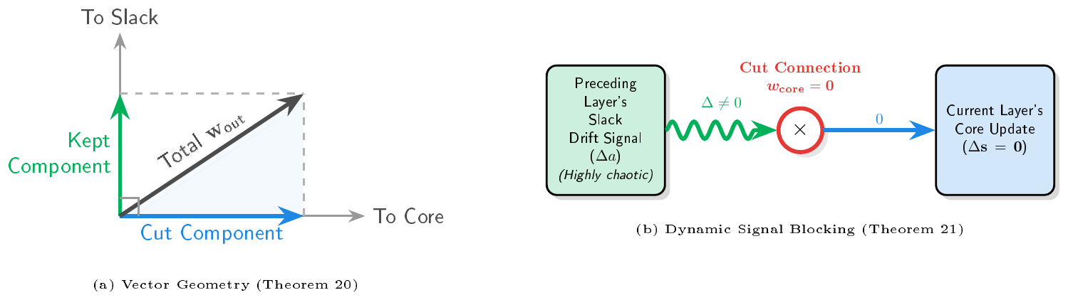
H.1 Algorithmic Axioms and Partitioning of Neurons

Here we formally define how DEFT partitions neurons into the peripheral slack and universal core. We also present a few axioms that merely mirror the mechanisms designated in the DEFT algorithm itself. These axioms do not impose any extra assumptions or restrictions on DEFT beyond the entirety of the algorithm itself.

########## {caption="Definition 15: Neurons Partition"}

For any intermediate layer $l$ containing a set of active neurons $\mathcal{I}^{(l)}$, a continuous capacity threshold $\tau^{(l)} > 0$ divides the layer into two disjoint functional subsets:

$ \begin{aligned} \mathcal{N}^{(l)}{\text{core}} &= {i \in \mathcal{I}^{(l)} \mid |f_i|{\mathcal{H}^{(l)}} > \tau^{(l)}} \ \mathcal{N}^{(l)}{\text{slack}} &= {j \in \mathcal{I}^{(l)} \mid |f_j|{\mathcal{H}^{(l)}} \le \tau^{(l)}} \end{aligned} $

########## {caption="Axiom 16: The Algorithmic Structural Mask"}

At initialization $t=0$, DEFT prevents cross-subset interference by severing the projections from the upstream slack subset to the downstream core. For any weight $w_{u, j}$ from an upstream slack neuron $j \in \mathcal{N}^{(l)}{\text{slack}}$ to a downstream core neuron $u \in \mathcal{N}^{(l+1)}{\text{core}}$, the mask $\boldsymbol{M}$ enforces $w_{u, j} = 0$.

########## {caption="Axiom 17: The Gradient Elasticity"}

During target optimization $t>0$, the parameter update for any parameter vector $\boldsymbol{\theta}_k$ belonging to a destination neuron $k$ is governed by:

$ \frac{\partial \boldsymbol{\theta}k}{\partial t} = E_k \cdot \nabla{\boldsymbol{\theta}k} \mathcal{L}{\text{target}}\tag{100} $

where $E_k \in {0, 1}$ is the elasticity multiplier. Slack neurons are fully plastic $E_j = 1 , \forall j \in \mathcal{N}{\text{slack}}$ and core neurons are strictly frozen $E_u = 0 , \forall u \in \mathcal{N}{\text{core}}$.

########## {caption="Axiom 18: The Merged-Vessel Release"}

When the continuous encoder collapses redundant neurons into a rank-1 parent operator, DEFT assigns full plasticity $E_j = 1$ to the structurally released child neurons.

H.2 Layer-to-Layer Bounding Framework

We now establish a rigorous bound on the structural distortion, decoupled entirely from target parameter drift.

########## {caption="Assumption 19: Bipartite Separability"}

Let the pre-activation $y_u$ of a downstream core neuron $u \in \mathcal{N}^{(l+1)}{\text{core}}$ be a linear combination of upstream activations $g_k(\boldsymbol{x}) = \Psi(y_k(\boldsymbol{x}))$ for $k \in \mathcal{I}^{(l)}$, governed by parameterized weights $w{u, k}$ and unparameterized identity connections denoted by an adjacency indicator $\mathbb{I}{u, k} \in {0, 1}$. We assume that for all upstream slack neurons $j \in \mathcal{N}^{(l)}{\text{slack}}$, the network identity routing is strictly zero:

$ \mathbb{I}{u, j} = 0 \quad \forall j \in \mathcal{N}^{(l)}{\text{slack}}, \forall u \in \mathcal{N}^{(l+1)}_{\text{core}}\tag{101} $

This ensures that the mask strictly dictates inter-subset signal flow.

Remark on Feed-Forward Architectures:

For purely sequential architectures (e.g., standard MLPs or VGG), $\mathbb{I}_{u, k} \equiv 0$ globally. This assumption only becomes non-trivial in architectures with unparameterized residual connections (e.g., ResNets), where an identity mapping could bypass the mask if the architecture cross-wired the subsets.

########## {caption="Theorem 20: The Static Initialization Shock Bound"}

Let $g_k(\boldsymbol{x}) \triangleq \Psi(y_k(\boldsymbol{x}))$, and let $\boldsymbol{s}{\text{core}}(\boldsymbol{x}) \triangleq \sum{k \in \mathcal{I}^{(l)}} \boldsymbol{w}{\text{core}, k} , g_k(\boldsymbol{x})$ be the input to the downstream core. The initialization mask $\boldsymbol{M}$ introduces a distortion $\Delta \boldsymbol{s}{\text{core}}^{\text{init}}(\boldsymbol{x}) \triangleq \sum_{j \in \mathcal{N}{\text{slack}}^{(l)}} \boldsymbol{w}{\text{core}, j} g_j(\boldsymbol{x})$ bounded over $P_\mathcal{X}$ by:

$ \left\lVert\Delta \boldsymbol{s}{\text{core}}^{\text{init}}\right\rVert{\mathcal{H}^{(l)}} \le | \mathcal{N}_{\text{slack}}^{(l)}| , \tau^{(l)}\tag{102} $

Proof: By Assumption 19, $\boldsymbol{s}_{\text{core}}(\boldsymbol{x})$ decomposes strictly over the parameterized upstream subsets:

$ \boldsymbol{s}{\text{core}}(\boldsymbol{x}) = \sum{i \in \mathcal{N}{\text{core}}^{(l)}} g_i(\boldsymbol{x}) , \boldsymbol{w}{\text{core}, i} + \sum_{j \in \mathcal{N}{\text{slack}}^{(l)}} g_j(\boldsymbol{x}) , \boldsymbol{w}{\text{core}, j}\tag{103} $

where $\boldsymbol{w}{\text{core}, k}$ is the sub-vector of structural weights connecting upstream neuron $k$ to the downstream core. By Axiom 16, DEFT enforces $\boldsymbol{w}{\text{core}, j} = \boldsymbol{0} , \forall j \in \mathcal{N}_{\text{slack}}^{(l)}$. The resulting functional distortion evaluates to the severed projections:

$ \Delta \boldsymbol{s}{\text{core}}^{\text{init}}(\boldsymbol{x}) = \sum{j \in \mathcal{N}{\text{slack}}^{(l)}} g_j(\boldsymbol{x}) , \boldsymbol{w}{\text{core}, j}\tag{104} $

Applying the triangle inequality in $\mathcal{H}^{(l)}$ yields:

$ \left\lVert\Delta \boldsymbol{s}{\text{core}}^{\text{init}}\right\rVert{\mathcal{H}^{(l)}} \le \sum_{j \in \mathcal{N}{\text{slack}}^{(l)}} \left\lVert\boldsymbol{w}{\text{core}, j}\right\rVert_2 \left\lVert g_j\right\rVert_{\mathcal{H}_{\text{in}}^{(l)}}\tag{105} $

By Definition 99, $\left\lVert g_j\right\rVert_{\mathcal{H}{\text{in}}^{(l)}} = \sqrt{K(j, j)}$. Furthermore, because $\boldsymbol{w}{\text{out}, j} = \boldsymbol{w}{\text{core}, j} \oplus \boldsymbol{w}{\text{slack}, j}$, its Euclidean norm bounds its sub-vectors: $\left\lVert\boldsymbol{w}{\text{core}, j}\right\rVert_2 \le \left\lVert\boldsymbol{w}{\text{out}, j}\right\rVert_2$. Substituting these properties gives:

$ \left\lVert\Delta \boldsymbol{s}{\text{core}}^{\text{init}}\right\rVert{\mathcal{H}^{(l)}} \le \sum_{j \in \mathcal{N}{\text{slack}}^{(l)}} \left\lVert\boldsymbol{w}{\text{out}, j}\right\rVert_2 \sqrt{K(j, j)} = \sum_{j \in \mathcal{N}{\text{slack}}^{(l)}} |f_j|{\mathcal{H}^{(l)}}\tag{106} $

By Definition 15, the capacity of every slack neuron satisfies $|f_j|_{\mathcal{H}^{(l)}} \le \tau^{(l)}$. Therefore, the functional distortion is strictly bounded by:

$ \left\lVert\Delta \boldsymbol{s}{\text{core}}^{\text{init}}\right\rVert{\mathcal{H}^{(l)}} \le \sum_{j \in \mathcal{N}{\text{slack}}^{(l)}} \tau^{(l)} = \tau^{(l)} , | \mathcal{N}{\text{slack}}^{(l)}|\tag{107} $

H.2.1 Dynamic Decoupling

The dynamic decoupling of the core emerges as a direct consequence of Axiom 17.

########## {caption="Theorem 21: Dynamic Decoupling"}

During target fine-tuning $t>0$, the operators $f_i^{(l)}$ of all neurons within the core experience zero dynamic deviation:

$ \forall , l , , , i \in \mathcal{N}^{(l)}{\text{core}} , ;, \left\lVert f_i^{(l), (t)} - f_i^{(l), (0)}\right\rVert{\mathcal{H}^{(l)}} = 0\tag{108} $

Proof: We proceed by structural induction over the network layers.

Base Case: The input $\boldsymbol{x} \sim P_\mathcal{X}$ is a static anchor unmodified by optimization $\Delta \boldsymbol{x} = \boldsymbol{0}$.

Inductive Step: Assume that for layer $l$, the core functional mappings exhibit zero drift: $g_i^{(t)}(\boldsymbol{x}) = g_i^{(0)}(\boldsymbol{x})$ for all $i \in \mathcal{N}_{\text{core}}^{(l)}$.

The dynamic deviation of the signal injected into the downstream core of layer $l+1$ at time $t$ is defined by $\Delta \boldsymbol{s}{\text{core}}(\boldsymbol{x}) = \boldsymbol{s}{\text{core}}^{(t)}(\boldsymbol{x}) - \boldsymbol{s}_{\text{core}}^{(0)}(\boldsymbol{x})$. Expanding this difference over the core and slack subsets yields:

$ \Delta \boldsymbol{s}{\text{core}}(\boldsymbol{x}) = \sum{i \in \mathcal{N}{\text{core}}^{(l)}} \left(\boldsymbol{w}{\text{core}, i}^{(t)} g_i^{(t)}(\boldsymbol{x}) - \boldsymbol{w}{\text{core}, i}^{(0)} g_i^{(0)}(\boldsymbol{x}) \right) + \sum{j \in \mathcal{N}{\text{slack}}^{(l)}} \left(\boldsymbol{w}{\text{core}, j}^{(t)} g_j^{(t)}(\boldsymbol{x}) - \boldsymbol{w}_{\text{core}, j}^{(0)} g_j^{(0)}(\boldsymbol{x}) \right)\tag{109} $

For the first summation, Axiom 17 freezes downstream core weights $E_u = 0 \implies \boldsymbol{w}{\text{core}, i}^{(t)} = \boldsymbol{w}{\text{core}, i}^{(0)}$, and the inductive hypothesis guarantees $g_i^{(t)}(\boldsymbol{x}) = g_i^{(0)}(\boldsymbol{x})$. The first summation is therefore zero.

For the second summation, Axiom 16 severs cross-subset weights at initialization $\boldsymbol{w}{\text{core}, j}^{(0)} = \boldsymbol{0}$. Because $E_u = 0$, these structural weights receive zero gradient updates and remain zero $\boldsymbol{w}{\text{core}, j}^{(t)} = \boldsymbol{0}$. Thus, the second summation evaluates to zero irrespective of the slack drift $g_j^{(t)}$.

Consequently, $\Delta \boldsymbol{s}_{\text{core}}(\boldsymbol{x}) \equiv \boldsymbol{0}$. Since the downstream core parameters $\boldsymbol{\theta}u \in {\boldsymbol{w}{\text{in}, u}, b_u, \gamma_u, \beta_u}$ are also frozen $E_u = 0$, the downstream core mappings experience zero drift $g_u^{(t)}(\boldsymbol{x}) = g_u^{(0)}(\boldsymbol{x})$. By induction, the target learning is decoupled from the core representation across all layers.

Remark on Covariate Shift:

Theorem 21 guarantees the immutability of the core operators relative to the source distribution anchor $P_\mathcal{X}$. In practice, the network processes novel target data $\mathcal{D}_T$ during fine-tuning. Consequently, empirical activations flowing through the core will inevitably shift due to standard covariate shift, not parameter degradation. DEFT ensures that any shift in downstream representations is driven entirely by the target data itself, free from the compounding noise of parameter degradation. This preserves foundational knowledge as an uncorrupted lens for processing new domains.

########## {caption="Corollary 22: Cumulative Masking-Induced Bound"}

Assuming a masking-based reduction without feature merging, the global structural distortion $D_{\text{global}}^{\text{mask}}$ evaluates as the cumulative sum of normalized layer-wise distortions. Normalizing the initialization shock at each layer by the downstream core capacity $E_{\text{core}}^{(l+1)} \triangleq \sum_{u \in \mathcal{N}{\text{core}}^{(l+1)}} |f_u|{\mathcal{H}^{(l+1)}}$, the total distortion is bounded by:

$ D_{\text{global}}^{\text{mask}} \triangleq \sum_{l=1}^{L-1} \frac{\left\lVert\Delta \boldsymbol{s}{\text{core}}^{\text{init}, (l+1)}\right\rVert{\mathcal{H}^{(l)}}}{E_{\text{core}}^{(l+1)}} \le \sum_{l=1}^{L-1} \left(\frac{| \mathcal{N}{\text{slack}}^{(l)}| \tau^{(l)}}{E{\text{core}}^{(l+1)}} \right)\tag{110} $

This confirms that source task degradation is strictly bounded by the chosen capacity thresholds, circumventing the exponential scaling issues of global Lipschitz constants.

H.3 Dynamic Resolution of Redundancy via Bounded Trade-off

A static capacity threshold evaluates functional volume in isolation, which ignores the redundancy trap where networks fragment a feature across multiple correlated neurons. To compress this redundant volume and avoid incorrectly locking it, DEFT employs HOPE's MERGE operation.

########## {caption="Proposition 23: Bounded Distortion of Merging"}

Consolidating $M$ correlated neurons into a rank-1 parent neuron guarantees the release of target optimization volume while bounding the distortion of the source representation.

Proof: Suppose $M$ correlated neurons ${f_m}_{m=1}^M$ are assigned to the core $E_m = 0$. By generating an optimal parent $f_p \in \mathcal{H}^{(l)}$, DEFT collapses $M$ copies into $1$ and frees $M-1$ child vessels. By Axiom 18, DEFT assigns these children full plasticity $E_j = 1$, successfully releasing the parameter space $\mathbb{R}^{(M-1) \times c}$ for optimization.

The distortion $\delta_k$ introduced by this operation is the composite projection error between the parent $f_p$ and its children ${f_m}_{m=1}^M$. Because the optimal parent minimizes this distance in $\mathcal{H}^{(l)}$, the error is upper-bounded by the sub-optimal projection to the null operator $f_p \equiv \boldsymbol{0}$:

$ \delta_k \triangleq \min_{f_p} \left(\sum_{m=1}^M |f_m - f_p|{\mathcal{H}^{(l)}}^2 \right)^{\frac{1}{2}} \le \left(\sum{m=1}^M |f_m - \boldsymbol{0}|_{\mathcal{H}^{(l)}}^2 \right)^{\frac{1}{2}}\tag{111} $

Applying the standard $\ell_p$-norm inequality $| \boldsymbol{x}|_2 \le | \boldsymbol{x}|_1$, we bound this sub-optimal projection by the linear sum of the child capacities:

$ \delta_k \le \sum_{m=1}^M |f_m|_{\mathcal{H}^{(l)}}\tag{112} $

Thus, the algorithm safely releases massive target parameter volume while the distortion remains strictly bounded by the initial capacities.

########## {caption="Corollary 24: The Unified Cumulative Bound"}

By the triangle inequality in $\mathcal{H}^{(l)}$, the total perturbation injected into the core of layer $l+1$ is bounded by the sum of the missing slack projections (Theorem 20) and the structural projection errors from $K^{(l)}$ merge operations. Because dynamic interference evaluates to zero via structural induction (Theorem 21), the global normalized functional distortion is bounded as:

$ D_{\text{global}}^{\text{total}} \triangleq \sum_{l=1}^{L-1} \frac{\left\lVert\Delta \boldsymbol{s}{\text{core}}^{(l+1)}\right\rVert{\mathcal{H}^{(l)}}}{E_{\text{core}}^{(l+1)}} \le \sum_{l=1}^{L-1} \left(\frac{| \mathcal{N}{\text{slack}}^{(l)}| \tau^{(l)} + \sum{k=1}^{K^{(l)}} \delta_{k}}{E_{\text{core}}^{(l+1)}} \right)\tag{113} $

where $\delta_k$ is the bounded projection error of the $k$-th merge operation. Therefore, DEFT releases target parameter volume while bounding cumulative source degradation to an algorithmically verifiable constant.

I. Algorithms

**Require:** Pre-trained model M, Target density rho(target)
**Initialize** CostManager()
// **PHASE 1: O(N²) Initialization**
**for** each layer L ∈ M **do**
  InitializeCaches(L) // Computes initial capacities and O(N²) geometry
  Anchor initial uncompressed capacity E₀(L)
**end for**
// **PHASE 2: True O(1) Greedy Scan**
**while** Density(M) > rho(target) **do**
  a* ← null, DR(min) ← ∞
  // *Evaluate all cached actions using live residual capacities*
  **for** each active layer L **do**
    $E_{\text{rem}} \gets \operatorname{GetResidualCapacity}(L)$ // Dynamic tracking of layer shrinkage
    N(live) ← L.ActiveCount() // Live layer width for unbiased normalization
    **for** each candidate c ∈ L.ActiveActions() // Prunes, Merges, Evicts **do**
      $\Delta P_{\text{static}} \gets \operatorname{GetStaticPayoff}(c)$ // Action-specific static payoff
      $\mathcal{J}_{\text{cost}} \gets \operatorname{ComputeDistortion}(c, E_{\text{rem}}, N_{\text{live}})$ // O(1) scalar arithmetic
      DR ← J(cost) / Delta P(static)
      **if** DR < DR(min) **then**
        DR(min) ← DR
        a* ← c
      **end if**
    **end for**
  **end for**
  // *Execution and Local Synthesis*
  ExecutePhysicalReduction(M, a*)
  UpdateResidualCapacity(a*.L, a*. J(cost))
  // *O(1) Local Recalculation (Strict intra-layer isolation)*
  **if** a*.type == MERGE **then**
    f(p) ← a*.parent
    Cache.UpdatePruneCapacity(f(p)) // Update solitary capacity for new parent
    **for** each f(neighbor) ∈ a*.L.ActiveNeurons() **do**
      $\text{geo}_{\text{new}} \gets \operatorname{PrecomputePairGeometry}(f_p, f_{\text{neighbor}})$
      Cache.Insert((f(p), f(neighbor)), geo(new))
    **end for**
  **end if**
  // ZERO downstream recalculation required due to the static Delta P approximation
**end while**
**return** M

**Require:** Executed compression action a* (contains action type, target layer(s) L, and targeted neurons)
$\epsilon \gets 10^{-12}$ // Numerical stability floor for capacity tracking
**if** a*.type == PRUNE **then**
  L ← a*.L
  f(vic) ← a*.victim
  Delta E ← Cache.GetPruneCapacity(f(vic))
  $L.E_{\text{rem}} \gets \max(L.E_{\text{rem}} - \Delta E, \epsilon)$
  L.RemoveNeuron(f(vic))
**else if** a*.type == MERGE **then**
  L ← a*.L
  f(i), f(j) ← a*.children
  f(p) ← a*.parent
  // Net flux: capacity of the extinguished children minus the new parent
  $\Delta E \gets \text{Cache}.\text{GetPruneCapacity}(f_i) + \text{Cache}.\text{GetPruneCapacity}(f_j) - \operatorname{ComputeCapacity}(f_p)$
  $L.E_{\text{rem}} \gets \max(L.E_{\text{rem}} - \Delta E, \epsilon)$
  L.RemoveNeuron(f(j)) // Child j is purged; Child i serves as the vessel for $f_p$
**else if** a*.type == EVICT **then**
  // Eviction targets all internal reduction layers within the residual pathway
  **for** each internal layer L ∈ a*.block **do**
    $L.E_{\text{rem}} \gets \epsilon$ // Pathway capacity forcibly collapsed
    L.ClearAllActiveNeurons() // All internal operators are projected to $\boldsymbol{0}$
  **end for**
**end if**

**Require:** Pre-trained source parameters θ(src), Source validation data D(s)(v)al, Target data D(t), Percentile threshold P
// **PHASE 1: Capacity Evaluation \& Core/Slack Partitioning**
**Merge Redundancies:** Use HOPE to compress highly correlated neurons into parent operators, freeing child vessels.
**Compute Capacities:** Calculate the functional capacity ‖f(i)‖H for all active neurons.
**Thresholding:** Determine global capacity threshold τ corresponding to the P-th percentile.
**for** each neuron i in the network **do**
  **if** ‖f(i)‖H > τ **and** neuron i is active **then**
    E(i) ← 0 // **Universal Core:** Freeze to protect source knowledge
  **else**
    E(i) ← 1 // **Plastic Slack:** Freed vessels and weak neurons learn target
  **end if**
**end for**
// **PHASE 2: Consistency at Initialization (The Structural Mask)**
Initialize target weights θ₀ ← θ(src).
**for** each weight w(u,j) connecting an upstream neuron j to a downstream neuron u **do**
  **if** E(j) = 1 **and** E(u) = 0 **then**
    M(u,j) ← 0 // Sever cross-connections to prevent Slack drift from entering Core
  **else**
    M(u,j) ← 1
  **end if**
**end for**
**Apply Mask:** $\theta_0 \gets \boldsymbol{M} \odot \theta_0$
// **PHASE 3: Elastic Target Fine-Tuning (Dynamic Decoupling)**
θ(t) ← θ₀, best(h)(score) ← -1
**for** epoch ∈ (1, …, FINETUNE(EPOCHS)) **do**
  **for** mini-batch $(\boldsymbol{x}, \boldsymbol{y}) \in \mathcal{D}_t^{\text{train}}$ **do**
    $\boldsymbol{g} \gets \nabla_{\theta_t} \mathcal{L}_{\text{target}}(\theta_t; \boldsymbol{x}, \boldsymbol{y})$ // Compute raw target gradients
    $\boldsymbol{g}_{\text{mod}} \gets \boldsymbol{E} \odot \boldsymbol{g}$ // Nullify gradients for frozen Core (E(i=0))
    $\theta_t \gets \operatorname{OptimizerStep}(\theta_t, \boldsymbol{g}_{\text{mod}})$ // Only plastic Slack updates
  **end for**
  *// Dual-Domain Evaluation (Harmonic Score Optimization)*
  $\text{Acc}_{\text{tgt}} \gets \operatorname{Evaluate}(\theta_t, \mathcal{D}_t^{\text{val}})$
  $\theta_{\text{src\_eval}} \gets \operatorname{MaskSlackDrift}(\theta_t, \theta_{\text{src}}, \boldsymbol{E})$ // Restore pristine Core / Mask out Slack drift
  $\text{Acc}_{\text{src}} \gets \operatorname{Evaluate}(\theta_{\text{src\_eval}}, \mathcal{D}_s^{\text{val}})$
  H-Score ← (2 · Acc(tgt) · Acc(src))/(Acc(tgt) + Acc(src))
  **if** H-Score > best(h)(score) **then**
    best(h)(score) ← H-Score
    θ(best) ← θ(t)
  **end if**
**end for**
**return** θ(best)

References

Section Summary: The references compile dozens of academic papers on neural network compression, pruning, and efficiency, drawing heavily from information theory ideas like minimizing description length and the information bottleneck. Many explore practical techniques for removing unnecessary weights or filters from deep models to reduce size and computational cost without major performance loss, including both classic methods from the 1980s and 1990s and recent work on data-free pruning and sparse architectures. The collection also connects these approaches to broader themes in representation learning, language modeling, and algorithmic compression.

[1] Rissanen, Jorma (1978). Modeling by shortest data description. Automatica. 14(5). pp. 465–471.

[2] Hinton, Geoffrey E and Van Camp, Drew (1993). Keeping the neural networks simple by minimizing the description length of the weights. In Proceedings of the Sixth Annual Conference on Computational Learning Theory. pp. 5–13.

[3] Delétang et al. (2023). Language Modeling Is Compression. arXiv. doi:10.48550/arxiv.2309.10668.

[4] Genewein et al. (2026). Algorithmic Compression via Pretrained Neural Networks. Entropy. 28. pp. 596. doi:10.3390/e28060596. https://doi.org/10.3390/e28060596.

[5] Mozer, Michael C and Smolensky, Paul (1988). Skeletonization: A Technique for Trimming the Fat from a Network via Relevance Assessment. In Advances in Neural Information Processing Systems. pp. .

[6] Tishby et al. (1999). The information bottleneck method. In The 37th Annual Allerton Conference on Communication, Control, and Computing. pp. 368–377.

[7] Shwartz-Ziv, Ravid and Tishby, Naftali (2017). Opening the black box of deep neural networks via information. arXiv preprint arXiv:1703.00810.

[8] Shwai He et al. (2026). Demystifying When Pruning Works via Representation Hierarchies. https://arxiv.org/abs/2603.24652. arXiv:2603.24652.

[9] Nguyen et al. (2026). Depth Fragility and Skeletal Universality: Decoupling Topology and Function in Deep Neural Networks. Mathematics. 14(9). pp. 1438. doi:10.3390/math14091438. https://www.mdpi.com/2227-7390/14/9/1438.

[10] Wang et al. (2025). Understanding Deep Representation Learning via Layerwise Feature Compression and Discrimination. Journal of Machine Learning Research. 26(47). pp. 1–71. http://jmlr.org.

[11] Yatin Dandi et al. (2025). The Computational Advantage of Depth in Learning High-Dimensional Hierarchical Targets. In The Thirty-ninth Annual Conference on Neural Information Processing Systems.

[12] Zhang et al. (2025). Saddle-to-Saddle Dynamics Explains A Simplicity Bias Across Neural Network Architectures. arXiv preprint arXiv:2512.20607. https://arxiv.org/abs/2512.20607.

[13] Ali Behrouz et al. (2026). Language Models Need Sleep: Learning to Self-Modify and Consolidate Memories. https://arxiv.org/abs/2606.03979. arXiv:2606.03979.

[14] Scholl, Carolin AND Rule, Michael E. AND Hennig, Matthias H. (2021). The information theory of developmental pruning: Optimizing global network architectures using local synaptic rules. PLOS Computational Biology. 17(10). pp. 1-23. doi:10.1371/journal.pcbi.1009458. https://doi.org/10.1371/journal.pcbi.1009458.

[15] Hidenori Tanaka et al. (2020). Pruning neural networks without any data by iteratively conserving synaptic flow. ArXiv. abs/2006.05467. https://api.semanticscholar.org/CorpusID:219558821.

[16] Hooker et al. (2019). What do compressed deep neural networks forget?. arXiv preprint arXiv:1911.05248.

[17] LeCun et al. (1989). Optimal brain damage. In Advances in Neural Information Processing Systems (NIPS).

[18] Hassibi, Babak and Storkey, David G (1992). Second order derivatives for network pruning: Optimal Brain Surgeon. In Advances in Neural Information Processing Systems.

[19] Frankle, Jonathan and Carbin, Michael (2019). The lottery ticket hypothesis: Finding sparse, trainable neural networks. In International Conference on Learning Representations.

[20] Molchanov et al. (2017). Pruning convolutional neural networks for resource efficient inference. In International Conference on Learning Representations.

[21] Luo et al. (2017). ThiNet: A filter level pruning method for deep neural network compression. In Proceedings of the IEEE International Conference on Computer Vision. pp. 5058–5066.

[22] Yin et al. (2020). Dreaming to distill: Data-free knowledge transfer via DeepInversion. In Proceedings of the IEEE/CVF Conference on Computer Vision and Pattern Recognition. pp. 8715–8724.

[23] Micaelli, Paul and Storkey, Amos J (2019). Zero-shot knowledge transfer via adversarial belief matching. In Advances in Neural Information Processing Systems.

[24] Han et al. (2015). Learning both weights and connections for efficient neural network. In Advances in neural information processing systems.

[25] He et al. (2017). Channel pruning for accelerating very deep neural networks. In Proceedings of the IEEE international conference on computer vision. pp. 1389–1397.

[26] Wen et al. (2016). Learning structured sparsity in deep neural networks. In Advances in Neural Information Processing Systems (NIPS).

[27] Li et al. (2017). Pruning filters for efficient convnets. In International Conference on Learning Representations (ICLR) Workshop.

[28] Liu et al. (2017). Learning efficient convolutional networks through network slimming. In Proceedings of the IEEE international conference on computer vision. pp. 2736–2744.

[29] Molchanov et al. (2019). Importance estimation for neural network pruning. In Proceedings of the IEEE/CVF conference on computer vision and pattern recognition. pp. 11264–11272.

[30] Singh, Sidak Pal and Alistarh, Dan (2020). WoodFisher: Efficient Second-Order Approximation for Neural Network Compression. In Advances in Neural Information Processing Systems. pp. 18098–18109.

[31] Blalock et al. (2020). What is the state of neural network pruning?. In Proceedings of Machine Learning and Systems. pp. 129–146.

[32] Renda et al. (2020). Comparing rewinding and fine-tuning in neural network pruning. In International Conference on Learning Representations.

[33] Badrinarayanan et al. (2015). Understanding symmetries in deep networks. arXiv preprint arXiv:1511.01029.

[34] Dinh et al. (2017). Sharp minima can generalize for deep nets. In International Conference on Machine Learning. pp. 1019–1028.

[35] Neyshabur et al. (2015). In search of the real inductive bias: On the role of implicit regularization in deep learning. In International Conference on Learning Representations.

[36] Lee et al. (2021). Layer-adaptive Sparsity for the Magnitude-based Pruning. In International Conference on Learning Representations. https://openreview.net/forum?id=H6ATjJ0TKdf.

[37] Huh et al. (2024). The Platonic Representation Hypothesis. arXiv preprint arXiv:2405.07987.

[38] Entezari et al. (2022). The role of permutation invariance in linear mode connectivity of neural networks. In International Conference on Learning Representations.

[39] Ainsworth et al. (2023). Git re-basin: Merging models modulo permutation symmetries. In International Conference on Learning Representations.

[40] Singh, Sidak Pal and Jaggi, Martin (2020). Model fusion via optimal transport. In Advances in Neural Information Processing Systems. pp. 22045–22055.

[41] Tatro et al. (2020). Optimizing mode connectivity via neuron alignment. In Advances in Neural Information Processing Systems. pp. 15300–15311.

[42] Stoica et al. (2024). Zipit! merging models from different tasks without training. In International Conference on Learning Representations.

[43] Srinivas, Suraj and Babu, R. Venkatesh (2015). Data-free parameter pruning for Deep Neural Networks. arXiv. doi:10.48550/arxiv.1507.06149.

[44] Yvinec et al. (2021). RED : Looking for Redundancies for Data-Free Structured Compression of Deep Neural Networks. arXiv. doi:10.48550/arxiv.2105.14797.

[45] Moreira et al. (2026). Native Hierarchical and Compositional Representations with Subspace Embeddings. In Proceedings of the 32nd ACM SIGKDD Conference on Knowledge Discovery and Data Mining (KDD '26). doi:10.1145/3770855.3817808.

[46] Bricken et al. (2023). Towards monosemanticity: Decomposing language models with dictionary learning. Transformer Circuits Thread.

[47] Hänni et al. (2024). Mathematical Models of Computation in Superposition. arXiv. doi:10.48550/arxiv.2408.05451.

[48] Mikolov et al. (2013). Efficient estimation of word representations in vector space. In 1st International Conference on Learning Representations, ICLR 2013.

[49] Pennington et al. (2014). Glove: Global vectors for word representation. In Proceedings of the 2014 conference on empirical methods in natural language processing (EMNLP). pp. 1532–1543.

[50] Park et al. (2023). The linear representation hypothesis and the geometry of large language models. arXiv preprint arXiv:2311.03658.

[51] Engels et al. (2024). Not All Language Model Features Are Linear. arXiv preprint arXiv:2405.14860.

[52] Huang et al. (2016). Deep networks with stochastic depth. In European Conference on Computer Vision (ECCV). pp. 646–661.

[53] Fan et al. (2020). Reducing Transformer Depth on Demand with Structured Dropout. In International Conference on Learning Representations (ICLR).

[54] Zoph, Barret and Le, Quoc V (2017). Neural architecture search with reinforcement learning. In International Conference on Learning Representations.

[55] Liu et al. (2019). DARTS: Differentiable Architecture Search. In International Conference on Learning Representations (ICLR).

[56] Veit, Andreas and Belongie, Serge (2018). Convolutional networks with adaptive inference graphs. In Proceedings of the European Conference on Computer Vision (ECCV). pp. 3–18.

[57] Wang et al. (2018). SkipNet: Learning Dynamic Routing in Convolutional Networks. In Proceedings of the European Conference on Computer Vision (ECCV). pp. 409–424.

[58] Lopes et al. (2017). Data-free knowledge distillation for deep neural networks. In NIPS Workshop on Machine Learning on the Phone and other Consumer Devices.

[59] Cai et al. (2020). Zeroq: A novel zero shot quantization framework. In Proceedings of the IEEE/CVF Conference on Computer Vision and Pattern Recognition. pp. 13169–13178.

[60] Nagel et al. (2019). Data-free quantization through weight equalization and bias correction. In Proceedings of the IEEE/CVF International Conference on Computer Vision. pp. 1325–1334.

[61] Jaynes, Edwin T (1957). Information theory and statistical mechanics. Physical review. 106(4). pp. 620.

[62] Ma et al. (2023). LLM-Pruner: On the Structural Pruning of Large Language Models. In Advances in Neural Information Processing Systems (NeurIPS). https://arxiv.org/abs/2305.11627.

[63] Neal, Radford M (1996). Bayesian learning for neural networks. Springer Science & Business Media.

[64] Lee et al. (2018). Deep neural networks as gaussian processes. In International Conference on Learning Representations.

[65] Jacot et al. (2018). Neural tangent kernel: Convergence and generalization in neural networks. In Advances in neural information processing systems.

[66] Yang, Greg (2019). Tensor programs i: Wide feedforward or recurrent neural networks of any architecture are gaussian processes. In Advances in Neural Information Processing Systems.

[67] Yosinski et al. (2014). How transferable are features in deep neural networks?. In Advances in neural information processing systems.

[68] Hu et al. (2022). LoRA: Low-Rank Adaptation of Large Language Models. In International Conference on Learning Representations (ICLR).

[69] Houlsby et al. (2019). Parameter-efficient transfer learning for NLP. In International Conference on Machine Learning. pp. 2790–2799.

[70] Grossberg, Stephen (1987). Competitive learning: From interactive activation to adaptive resonance. Cognitive Science. 11(1). pp. 23–63.

[71] Kirkpatrick et al. (2017). Overcoming catastrophic forgetting in neural networks. Proceedings of the national academy of sciences. 114(13). pp. 3521–3526.

[72] Zenke et al. (2017). Continual learning through synaptic intelligence. In International conference on machine learning. pp. 3987–3995.

[73] McClelland et al. (1995). Why there are complementary learning systems in the hippocampus and neocortex: insights from the successes and failures of connectionist models of learning and memory.. Psychological Review. 102(3). pp. 419–457.

[74] Kumaran et al. (2016). What learning systems do intelligent agents need? Complementary learning systems theory updated. Trends in Cognitive Sciences. 20(7). pp. 512–534.

[75] Lingjing Kong et al. (2026). From Reasoning Traces to Reusable Modules: Understanding Compositional Generalization in Language Model Reasoning. https://arxiv.org/abs/2606.18089. arXiv:2606.18089.

[76] Saha et al. (2021). Gradient Projection Memory for Continual Learning. In International Conference on Learning Representations (ICLR).

[77] Zeng et al. (2019). Continual learning of context-dependent processing in neural networks. Nature Machine Intelligence. 1(8). pp. 364–372.

[78] Yang et al. (2025). LoRA-Null: Directing Parameter-Efficient Adaptation into Orthogonal Null-Spaces. In Proceedings of the International Conference on Machine Learning (ICML).

[79] HuggingFace Research Team et al. (2026). Orthogonal Subspace Fine-Tuning (OSF): A Unified Framework for Interference-Free PEFT. arXiv preprint arXiv:2602.04519.

[80] Andrei et al. (2023). Rapid compensatory plasticity revealed by dynamic correlated activity in monkeys in vivo. Nature Neuroscience. 26(11). pp. 1960–1969.

[81] Bau et al. (2017). Network dissection: Quantifying interpretability of deep visual representations. In Proceedings of the IEEE conference on computer vision and pattern recognition. pp. 6541–6549.

[82] Morcos et al. (2018). On the importance of single directions for generalization. In International Conference on Learning Representations.

[83] Olah et al. (2020). Zoom In: An Introduction to Circuits. Distill. doi:10.23915/distill.00024.001. https://distill.pub/2020/circuits/zoom-in.

[84] Neyshabur et al. (2017). Exploring generalization in deep learning. In Advances in neural information processing systems.

[85] Diaconis, Persi and Freedman, David (1984). Asymptotics of graphical projections. The Annals of Statistics. pp. 793–815.

[86] Hanin, Boris and Rolnick, David (2018). How to Start Training: The Effect of Initialization and Architecture. In Advances in Neural Information Processing Systems. pp. 571–581.

[87] Goyal et al. (2017). Accurate, large minibatch SGD: Training ImageNet in 1 hour. arXiv preprint arXiv:1706.02677.

[88] He et al. (2016). Identity mappings in deep residual networks. In European conference on computer vision (ECCV). pp. 630–645.

[89] Camacho, Eduardo F and Bordons, Carlos Alba (2013). Model predictive control. Springer Science & Business Media.

[90] Bertsekas, Dimitri P (2012). Dynamic programming and optimal control: Volume I. Athena scientific.

[91] Karp, Richard M (1972). Reducibility among combinatorial problems.

[92] Garey, Michael R and Johnson, David S (1979). Computers and intractability: A guide to the theory of NP-completeness. W. H. Freeman and Company.

[93] Dantzig, George B (1957). Discrete-variable extremum problems. Operations research. 5(2). pp. 266–288.

[94] Billot et al. (2024). The language network ages well: Preserved selectivity, lateralization, and within-network functional synchronization in older brains. bioRxiv.

[95] Blank et al. (2016). A functional MRI investigation of the language network. Journal of Neurophysiology. 116(4). pp. 1968–1984.

[96] Casto, Elena and Fedorenko, Evelina (2026). Cerebellar language hubs: Functional segregation of linguistic processing from motor and cognitive domains. Nature Neuroscience. 29(2). pp. 145–158.

[97] Kimmel et al. (2026). Neural representations supporting generalization under continual learning. bioRxiv. doi:10.1101/2026.01.07.698044. https://www.biorxiv.org/content/10.64898/2026.01.07.698044.

[98] Martin, Charles H and Mahoney, Michael W (2021). Implicit self-regularization in deep neural networks: Evidence from random matrix theory and implications for learning. Journal of Machine Learning Research. 22(165). pp. 1–73.

[99] El Cheairi et al. (2026). Theoretical Compression Bounds for Wide Multilayer Perceptrons. In 39th Annual Conference on Learning Theory. pp. 1–59.

[100] Mallya, Arun and Lazebnik, Svetlana (2018). PackNet: Adding Multiple Tasks to a Single Network by Iterative Pruning. In Proceedings of the IEEE Conference on Computer Vision and Pattern Recognition (CVPR). pp. 7765–7773.

[101] Scardapane et al. (2017). Group sparse regularization for deep neural networks. Neurocomputing. 241. pp. 81–89.

[102] Jaeger, Herbert (2014). Controlling Recurrent Neural Networks by Conceptors. arXiv. doi:10.48550/arxiv.1403.3369.

[103] Wang et al. (2021). Training Networks in Null Space of Feature Covariance for Continual Learning. 2021 IEEE/CVF Conference on Computer Vision and Pattern Recognition (CVPR). pp. 184–193. doi:10.1109/cvpr46437.2021.00025.

[104] Zhou et al. (2026). TACO: Temporal Consensus Optimization for Continual Neural Mapping. arXiv preprint arXiv:2602.04516.

[105] Qiu et al. (2024). Continual Learning in the Frequency Domain. In Advances in Neural Information Processing Systems (NeurIPS).

[106] Xie et al. (2025). AdaDARE-$\gamma$: Balancing Stability and Plasticity in Multi-modal LLMs through Efficient Adaptation. In Proceedings of the IEEE/CVF Conference on Computer Vision and Pattern Recognition (CVPR).

[107] Islam et al. (2025). Latest Advancements Towards Catastrophic Forgetting under Data Scarcity: A Comprehensive Survey on Few-Shot Class Incremental Learning. arXiv preprint arXiv:2502.08209.

[108] Krizhevsky, Alex (2009). Learning Multiple Layers of Features from Tiny Images. pp. 32–33. https://www.cs.toronto.edu/~kriz/learning-features-2009-TR.pdf.

[109] Netzer et al. (2011). Reading Digits in Natural Images with Unsupervised Feature Learning. In NIPS Workshop on Deep Learning and Unsupervised Feature Learning.

[110] Frankle et al. (2021). Training BatchNorm and Only BatchNorm: On the Expressive Power of Random Features in CNNs. In International Conference on Learning Representations.

[111] Cho, Youngmin and Saul, Lawrence (2009). Kernel Methods for Deep Learning. In Advances in Neural Information Processing Systems. pp. . https://proceedings.neurips.cc/paper_files/paper/2009/file/5751ec3e9a4feab575962e78e006250d-Paper.pdf.