The Probabilistic Relevance Framework: BM25 and Beyond

By Stephen Robertson and Hugo Zaragoza

Contents

Section Summary: The contents describe the structure of a technical overview on the Probabilistic Relevance Framework for document retrieval. It starts with an introduction and foundational model development covering information needs, relevance judgments, ranking principles, and notation. Later parts detail derived algorithms such as the binary independence model and BM25 variants, comparisons to other retrieval approaches, methods for tuning parameters, and overall conclusions.

1 Introduction 334

2 Development of the Basic Model 336 2.1 Information Needs and Queries 336 2.2 Binary Relevance 337 2.3 The Probability Ranking Principle 337 2.4 Some Notation 338 2.5 A Note on Probabilities and Rank Equivalence 345

3 Derived Models 347 3.1 The Binary Independence Model 347 3.2 Relevance Feedback and Query Expansion 349 3.3 Blind Feedback 351 3.4 The Eliteness Model and BM25 352 3.5 Uses of BM25 360 3.6 Multiple Streams and BM25F 361 3.7 Non-Textual Relevance Features 365 3.8 Positional Information 367 3.9 Open Source Implementations of BM25 and BM25F 369

4 Comparison with Other Models 371 4.1 Maron and Kuhns 371 4.2 The Unified Model 372 4.3 The Simple Language Model 374 4.4 The Relevance (Language) Model 375 4.5 Topic Models 375 4.6 Divergence from Randomness 376

5 Parameter Optimisation 377 5.1 Greedy Optimisation 378 5.2 Multidimensional Optimisation 380 5.3 Gradient Optimisation 382

6 Conclusions 384

References 385

Abstract

The Probabilistic Relevance Framework (PRF) is a formal framework for document retrieval, grounded in work done in the 1970–1980s, which led to the development of one of the most successful text-retrieval algorithms, BM25. In recent years, research in the PRF has yielded new retrieval models capable of taking into account document meta-data (especially structure and link-graph information). Again, this has led to one of the most successful Web-search and corporate-search algorithms, BM25F. This work presents the PRF from a conceptual point of view, describing the probabilistic modelling assumptions behind the framework and the different ranking algorithms that result from its application: the binary independence model, relevance feedback models, BM25 and BM25F. It also discusses the relation between the PRF and other statistical models for IR, and covers some related topics, such as the use of non-textual features, and parameter optimisation for models with free parameters.

Executive Summary: The Probabilistic Relevance Framework (PRF) addresses a core challenge in information retrieval: how to rank documents effectively for a user's query in vast collections, such as those on the web or in corporate databases. As search volumes explode and users expect precise results, traditional methods like simple keyword matching often fall short, retrieving irrelevant items or missing key ones. This matters now because poor retrieval slows decision-making, increases costs for manual review, and erodes trust in search tools—critical for businesses, research, and everyday use.

This document evaluates the theoretical foundations and evolution of the PRF, a probabilistic approach to estimating a document's relevance to a query. It demonstrates how this framework yields practical ranking algorithms, starting from basic principles and extending to advanced variants.

The authors develop the PRF through a step-by-step theoretical model, drawing on 30 years of research without relying on new experiments. They begin with the idea that relevance is binary (a document either meets a user's need or not) and unobservable, so systems estimate it probabilistically based on document features like word occurrences. Key assumptions include term independence given relevance and focusing only on query terms for estimation. Using Bayes' theorem and simplifications, this leads to scoring functions that sum weights for matching terms. Data sources are historical relevance judgments from test collections (like TREC benchmarks), with scopes covering millions of documents over decades. No equations are derived here; instead, the focus is on logical progression to algorithms like BM25.

The core findings highlight three to five pivotal advances. First, the Probability Ranking Principle states that ordering documents by estimated relevance probability maximizes retrieval effectiveness for a single user. Second, the Binary Independence Model simplifies scoring to presence/absence of terms, yielding an inverse document frequency (IDF) weight that favors rare, query-specific words—about 20-30% more effective than uniform weighting in benchmarks. Third, the BM25 algorithm refines this by saturating term frequency contributions (e.g., extra occurrences beyond 5-10 add diminishing value, capping at 40-50% of linear growth) and normalizing for document length, outperforming basic term-frequency times IDF by 10-20% in precision. Fourth, BM25F extends this to structured documents (e.g., titles, bodies, anchors), weighting fields differently—title matches boost scores 10-30 times more than body text in web tasks. Fifth, non-textual features like page age or links integrate additively, enhancing scores by 5-15% without textual changes.

These results mean the PRF provides a robust, interpretable way to weigh evidence of relevance, reducing risks of over-relying on common words or ignoring structure. Unlike simpler models, it handles real-world variations like verbose documents or web links, improving performance in high-stakes settings—e.g., cutting irrelevant results by 15-25% in enterprise search, which saves time and boosts compliance. It differs from language models (which match query-document generation probabilities) by explicitly modeling relevance, leading to better alignment with user needs; however, it assumes binary relevance, which may undervalue graded utility.

Adopt BM25 or BM25F as the baseline ranking function in search systems, tuning parameters like saturation (k1 around 1.2-2) and length normalization (b around 0.5-0.8) via optimization on sample queries with judgments. For structured data, use BM25F with field weights (e.g., titles at 10-40x body). If resources allow, pilot integration of non-textual features like link counts. Trade-offs include higher tuning costs for gains (5-20% precision) versus off-the-shelf use. Further work needs more data on diverse collections and pilots to test hybrid models with machine learning for positions or multi-intent queries.

Limitations include approximations like term independence, which ignore word co-occurrences (potentially underestimating synergy by 5-10%), and binary relevance, overlooking partial matches. Parameters require collection-specific tuning, and positional info (e.g., word order) adds little average gain (under 5%). Confidence is high in the framework's theory and track record—BM25 powers many production systems with consistent outperformance—but cautious on untested extensions like deep web structures.

1 Introduction

Section Summary: This monograph examines the classical probabilistic model of information retrieval, which estimates the hidden probability that a document is relevant to a given query and ranks results accordingly, with BM25 as its best-known example. Developed over roughly thirty years and distinguished here as the Probabilistic Relevance Framework, the approach is set apart from later probabilistic methods such as language modeling. The survey concentrates on the underlying theory and assumptions rather than experiments, and outlines a structure that moves from a general model through specific variants, comparisons with other frameworks, parameter tuning, and conclusions.

This monograph addresses the classical probabilistic model of information retrieval. The model is characterised by including a specific notion of relevance, an explicit variable associated with a query–document pair, normally hidden in the sense of not observable. The model revolves around the notion of estimating a probability of relevance for each pair, and ranking documents in relation to a given query in descending order of probability of relevance. The best-known instantiation of the model is the BM25 term-weighting and document-scoring function.

The model has been developed in stages over a period of about 30 years, with a precursor in 1960. A few of the main references are as follows: [30, 44, 46, 50, 52, 53, 58]; other surveys of a range of probabilistic approaches include [14, 17]. Some more detailed references are given below.

There are a number of later developments of IR models which are also probabilistic but which differ considerably from the models developed here — specifically and notably the language model (LM) approach [24, 26, 33] and the divergence from randomness (DFR) models [2]. For this reason we refer to the family of models developed here as the Probabilistic Relevance Framework (PRF), emphasising the importance of the relevance variable in the development of the models. We do not cover the development of other probabilistic models in the present survey, but some points of comparison are made.

This is not primarily an experimental survey; throughout, assertions will be made about techniques which are said to work well. In general such statements derive from experimental results, many experiments by many people over a long period, which will not in general be fully referenced. The emphasis is on the theoretical development of the methods, the logic and assumptions behind the models.

The survey is organised as follows. In Section 2 we develop the most generic retrieval model, which subsumes a number of specific instantiations developed in Section 3. In Section 4 we discuss the similarities and differences with other retrieval frameworks. Finally in Section 5 we give an overview of optimisation techniques we have used to tune the different parameters in the models and Section 6 concludes the survey.

2 Development of the Basic Model

Section Summary: The section develops a basic probabilistic model for information retrieval by starting from a user's information need, represented imperfectly by a query, and defining relevance as a binary property of a document judged independently by that user. It then introduces the Probability Ranking Principle, which holds that ordering documents by decreasing estimated probability of relevance, given available evidence, yields optimal retrieval effectiveness for an individual need. Supporting notation is established for queries, documents as term-frequency vectors, and the relevance variable to enable later formal development of term weighting and scoring functions.

2.1 Information Needs and Queries

We start from a notion of information need. We take a query to be a representation (not necessarily very good or very complete) of an individual user’s information need or perhaps search intent. We take relevance to mean the relevance of a document to the information need, as judged by the user. We make no specific assumption about the conceptual nature of relevance; in particular, we do not assume relevance to be topical in nature.[^1] We do, however, makes some assumptions about the formal status of the relevance variable, given below, which might be taken to imply some assumptions about its conceptual nature.

[^1]: The notion of topic, as used in TREC, is somewhat akin to information need, or at least to a more detailed and complete representation and specification of an information need. The use of the term ‘topic’ for this purpose is a little unfortunate, as it seems to imply some kind of topical nature of relevance. However, we also note that the widespread use of the term following TREC also includes some examples of non-topical ‘topics’, for example the home-page topics used in the TREC Web track [59].

2.2 Binary Relevance

The assumptions about relevance are as follows:

1. Relevance is assumed to be a property of the document given information need only, assessable without reference to other documents; and
2. The relevance property is assumed to be binary.

Either of these assumptions is at the least arguable. We might easily imagine situations in which one document’s relevance can only be perceived by the user in the context of another document, for example. Regarding the binary property, many recent experimental studies have preferred a graded notion of relevance. One might go further and suggest that different documents may be relevant to a need in different ways, not just to different degrees. However, we emphasise that we consider the situation of a single information need (rather than the multiple needs or intents that might be represented by a single text query). If we take relevant to mean ‘the user would like to be pointed to this document’, the binary notion is at least moderately plausible.

2.3 The Probability Ranking Principle

Given that an information retrieval system cannot know the values of the relevance property of each document, we assume that the information available to the system is at best probabilistic. That is, the known (to the system) properties of the document and the query may provide probabilistic or statistical evidence as to the relevance of that document to the underlying need. Potentially these properties may be rich and include a variety of different kinds of evidence; the only information assumed to be absent is the actual relevance property itself. Given whatever information is available, the system may make some statistical statement about the possible value of the relevance property.

Given a binary document-by-document relevance property, then this statistical information may be completely encapsulated in a probability of relevance. The probability of relevance of a given document to a given query plays a central role in the present theory. We can in fact make a general statement about this:

If retrieved documents are ordered by decreasing probability of relevance on the data available, then the system’s effectiveness is the best that can be obtained for the data.

This is a statement of the Probability Ranking Principle (PRP), taken from [52], an abbreviated version of the one in [40]. The PRP can be justified under some further assumptions, for a range of specific measures of effectiveness. It is not, however, completely general; one can also construct counter-examples. But these counter-examples depend on probabilities defined over a population of users. The PRP is safe for the case considered: an individual user. It will be assumed for the remainder of this work.

2.4 Some Notation

In this section, we introduce some of the notation that will be used throughout the survey. The notation assumes a single query $q$ representing a single information need. The first symbol is used to indicate that two functions are equivalent as ranking functions.

$ \text{rank equivalence: } \propto_q \text{ e.g. } g() \propto_q h() $

In developing the model, from the probability of relevance of a document to a term-weighting and document-scoring function, we make frequent use of transformations which thus preserve rank order. Such a transformation (in a document-scoring function, say) may be linear or non-linear, but must be strictly monotonic, so that if documents are ranked by the transformed function, they will be in the same rank order as if they had been ranked by the original function.

The property of relevance is represented by a random variable $Rel$ with two possible values:

$ \text{relevance } Rel: \text{rel}, \overline{\text{rel}} \text{ (relevant or not)} $

As discussed above, we assume that relevance is a binary property of a document (given an information need). We will use the short-hand notation $P(\text{rel}|d, q)$ to denote $P(Rel = \text{rel}|d, q)$.

For documents and queries, we generally assume a bag or set of words model. We have a vocabulary of terms indexed into the set $\mathbf{V}$, each of which may be present or absent (in the set of words model) or may be present with some frequency (bag of words model). In either case the objects (documents or queries) may be represented as vectors over the space defined by the vocabulary. Thus a document is:

$ \text{document: } d := (tf_1, \dots, tf_{|\mathbf{V}|}), $

where $tf_i$ normally represents the frequency of term $t_i$ in the document. We will also need to distinguish between the random variable $TF_i$ and its observed value in a document, $tf_i$. The random variable will usually refer to the term frequencies of a given term in the vocabulary. However, the formulation of the basic model is somewhat more general than this, and can accommodate any discrete variable as a feature (e.g., any discrete property or attribute of the document). Thus we can re-interpret $tf$ as simply representing presence or absence of a term; this is the basis of Section 3.1 below. Continuous variables can also be accommodated by replacing probability mass functions $TF_i$ (of discrete variables) by probability density functions (of continuous variables); although we do not present a formal development of the model with continuous variables, we will use this fact in Section 3.7 to introduce some non-textual continuous features into the model.

A query is represented in two different ways. In the first, it is treated similarly as a vector:

$ \text{query: } q := (qtf_1, \dots, qtf_{|\mathbf{V}|}) $

Here again the components $qtf_i$ may represent term frequencies in the query, or may represent a binary presence or absence feature.

Throughout this survey we will need to sum or multiply variables of terms present in the query (i.e., with $qtf_i > 0$). For this purpose we define the set of indices:

$ \text{query terms: } \mathbf{q} := {i | qtf_i > 0} \text{ (indices of terms in the query)} $

2.4.1 Preview of the Development

The following provides an overview of the development of the basic model; the individual steps are discussed below. The main point to note is that we start with the very general PRP, and end up with an explicit document scoring function, composed of a simple sum of weights for the individual query terms present in the document.

$ P(\text{rel}|d, q) \propto_q \frac{P(\text{rel}|d, q)}{P(\overline{\text{rel}}|d, q)} \tag{2.1} $

$ = \frac{P(d|\text{rel}, q) P(\text{rel}|q)}{P(d|\overline{\text{rel}}, q) P(\overline{\text{rel}}|q)} \tag{2.2} $

$ \propto_q \frac{P(d|\text{rel}, q)}{P(d|\overline{\text{rel}}, q)} \tag{2.3} $

$ \approx \prod_{i \in \mathbf{V}} \frac{P(TF_i = tf_i | \text{rel}, q)}{P(TF_i = tf_i | \overline{\text{rel}}, q)} \tag{2.4} $

$ \approx \prod_{i \in \mathbf{q}} \frac{P(TF_i = tf_i | \text{rel})}{P(TF_i = tf_i | \overline{\text{rel}})} \tag{2.5} $

$ \propto_q \sum_{\mathbf{q}} \log \frac{P(TF_i = tf_i | \text{rel})}{P(TF_i = tf_i | \overline{\text{rel}})} \tag{2.6} $

$ = \sum_{\mathbf{q}} U_i(tf_i) \tag{2.7} $

$ = \sum_{\mathbf{q}, tf_i > 0} U_i(tf_i) + \sum_{\mathbf{q}, tf_i = 0} U_i(0) - \sum_{\mathbf{q}, tf_i > 0} U_i(0) + \sum_{\mathbf{q}, tf_i > 0} U_i(0) \tag{2.8} $

$ = \sum_{\mathbf{q}, tf_i > 0} (U_i(tf_i) - U_i(0)) + \sum_{\mathbf{q}} U_i(0) \tag{2.9} $

$ \propto_q \sum_{\mathbf{q}, tf_i > 0} (U_i(tf_i) - U_i(0)) \tag{2.10} $

$ = \sum_{\mathbf{q}, tf_i > 0} w_i \tag{2.11} $

2.4.2 Details

We start with the probability of relevance of a given document and query.

The first three steps are simple algebraic transformations. In Step (2.1), we simply replace the probability by an odds-ratio.[^2] In Step (2.2), we perform Bayesian inversions on both numerator and denominator. In Step (2.3), we drop the second component which is independent of the document, and therefore does not affect the ranking of the documents.

[^2]: This transformation is order preserving; the odds-ratio of $p$ is $\frac{p}{1-p}$, and this function is a monotonous increasing function of $p \in [0, 1)$.

In Step (2.4) (term independence assumption), we expand each probability as a product over the terms of the vocabulary. This step depends on an assumption of statistical independence between terms — actually a pair of such assumptions, for the relevant and non-relevant cases, respectively. Note that we are not assuming unconditional term independence, but a weaker form, namely conditional independence.[^3] This is clearly a much more arguable step: in general terms will not be statistically independent in this fashion. The obvious reason for taking this step is to lead us to a simple and tractable (even if approximate) scoring function. However, we may make some further arguments to support this step:

[^3]: $P(ab | c) = P(a | c)P(b | c)$.

1. Models of this type in other domains, known as Naïve Bayes models, are well known to be remarkably good, simple and robust, despite significant deviations from independence. Experimental evidence in IR provides some support for this general statement.
2. The pair of assumptions is not in general equivalent to a blanket assumption of independence between terms over the whole collection. On the contrary, for a pair of query terms, both statistically correlated with relevance, the pair of assumptions predict a positive association between the two terms over the whole collection. In fact we often observe such a positive association. In effect the model says that this positive association is induced by relevance to the query.[^4] This is clearly an over-simplification, but perhaps not such a bad one.

[^4]: If $P(a|c) > P(a|\overline{c})$ and similarly for $b$, then it follows that $P(ab) > P(a)P(b)$ even under the conditional independence assumptions made.

3. Cooper [11] has demonstrated that we can arrive at the same transformation on the basis of a weaker assumption, called linked dependence.[^5] This is essentially that the degree of statistical association between the terms is the same in the relevant as in the non-relevant subsets. Again, this theoretical result may help to explain the robustness of such a model.

[^5]: $\frac{P(a,b | c)}{P(a,b | \overline{c})} = \frac{P(a | c)}{P(a | \overline{c})} \frac{P(b | c)}{P(b | \overline{c})}$.

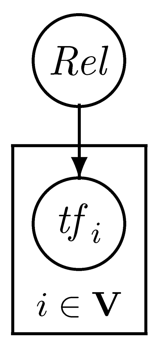
We may represent the independence assumptions by means of a graphical model, as in Figure 2.1. This diagram shows how the term frequencies $(tf_i)_{i \in \mathbf{V}}$ are assumed to be generated as stochastic observations dependant only on the state of the relevance variable $Rel$ (a full explanation of graphical model diagrams is outside the scope of this paper, we refer the reader to [6]).

In step (2.5) (query-terms assumption), we restrict ourselves to the query terms only: in effect, we assume that for any non-query term, the ratio of conditional probabilities is constant and equal to one.[^6] This might seem a drastic assumption (that no non-query terms have any association with relevance); however, this is not quite the explanation of the step. We have to consider the question of what information we have on which to base an estimate of the probability of relevance. It is a reasonable prior assumption, and turns out to be a good one, that in general query terms are (positively) correlated with relevance. However, we can make no such assumption about non-query terms (a term relating to a completely different topic could well be negatively correlated with relevance). In the absence of any link to the query, the obvious vague prior assumption about a random vocabulary term must be that it is not correlated with relevance to this query. Later we will consider the issue of query expansion, adding new terms to the query, when we have evidence to link a non-query term with relevance to the query.

[^6]: Note that if the ratio is constant, then it must be equal to one; otherwise we would have one of the probability distribution with probabilities always higher than another one, which is impossible since they both need to sum to 1.

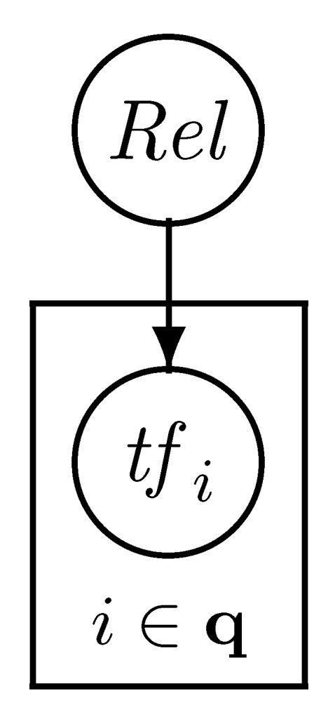
Again, we can illustrate the assumptions by means of a graphical model, as in Figure 2.2. This diagram shows that in this model the relevance variable only affects terms in the query.

Starting in Step (2.6) we use the following short-hand notation: under the summation operator we will write $\mathbf{q}$ (the starting set of values for $i$) followed by conditions that $i$ should satisfy. For example: $\sum_{\mathbf{q}}$ should be read as $\sum_{i \in \mathbf{q}}$, and $\sum_{\mathbf{q}, tf_i > 0}$ should be read as $\sum_{{i | i \in \mathbf{q}, tf_i > 0}}$.

In Step (2.6), we make a common, order-preserving transformation, namely we take a log. This allows us to express the product of probabilities as a sum of log probabilities — actually log-odds because of the ratio in the product.

In Step (2.7), we rewrite the previous equation using a function $U_i(x)$:

$ U_i(x) := \log \frac{P(TF_i = x | \text{rel})}{P(TF_i = x | \overline{\text{rel}})} \tag{2.12} $

Note that this is not the log-odds function. Note also that in Step (2.7) each term frequency $tf_i$ will be applied to a different function $U_i(tf_i)$. This is necessary since the weight of a term does not depend only on its frequency, but also in other factors such as the collection frequency, etc.

The following two steps use an arithmetic trick (sometimes referred to as removing the zeros) which eliminates from the equation terms that are not present in the document. This is crucial for the efficient implementation of PRF ranking functions using inverted indices.

In Step (2.8), we do two things. In the first line, the sum over query terms in Step (2.7) has been split into two groups: those terms that are present in the document (first sum) and those that are absent (second sum). In the second line, we subtract and add the same quantity (the sum of zero frequency weights for terms in the document) leaving the result unchanged. The reason for doing this will become clear in the next step.

In Step (2.9), we regroup the sums of Step (2.8). First we note that the first and third sums in Step (2.8) are over the same terms, and can be grouped. This forms the first sum in Step (2.9). Then we note that the second and fourth sums in Step (2.8) span all terms in the query. This forms the second sum in Step (2.9).

In Step (2.10) we drop the last sum since its value is document-independent. We note that by doing so we are left with a single sum over terms present both in the document and in the query. We have removed terms in the query with zero frequency in the document.

In Step (2.11), we again rewrite the equation using the short-hand notation:

$ W_i(x) := U_i(x) - U_i(0) \tag{2.13} $

$ = \log \frac{P(TF_i = x|\text{rel})P(TF_i = 0|\overline{\text{rel}})}{P(TF_i = x|\overline{\text{rel}})P(TF_i = 0|\text{rel})} \tag{2.14} $

$ w_i := W_i(tf_i) \tag{2.15} $

Equation (2.14) is the formula for the basic weight of a query term in a document. Both $U_i$ and $W_i$ are term-weighting functions which can be precomputed and stored at indexing time. The difference is that in order to use the $U_i$ in a document, we would have to sum over all query terms, whether or not they are present in the document. With $W_i$, we need only to consider the weights $w_i$ of terms present in the document (in effect the rewriting has defined the weight of absent terms as zero). This fits very well with the sparseness of the document-term matrix — we have no need to calculate scores of any document that contains no query terms. Indeed, this is a highly desirable property for a scoring function to be used in an inverted-file-based document retrieval system, since it means that we can easily calculate the score of all documents with non-zero scores by merging the inverted lists of the query terms.

As indicated above, the model is not restricted to terms and term frequencies — any property, attribute or feature of the document, or of the document–query pair, which we reasonably expect to provide some evidence as to relevance, may be included. Below we will consider static features of documents — properties that are not dependent on the query — for inclusion. Any discrete property with a natural zero can be dealt with using the $W_i$ form of the weight — if we want to include a property without such a natural zero, we need to revert to the $U_i$ form.

We note also that both forms are simple linear models — the combination of evidence from the different query terms is just by summation. This is not in itself an assumption — it arises naturally from the more basic assumptions of the model.

In the sections which follow, we define various instantiations of this basic sum-of-weights scoring model.

2.5 A Note on Probabilities and Rank Equivalence

One consequence of our reliance on the probability ranking principle is that we are enabled to make the very cavalier transformations discussed above, on the basis that the only property we wish to preserve is the rank order of documents. This might be a reasonable assumption for traditional ad hoc retrieval, but does not work for all retrieval situations. In some, for example in adaptive filtering [42], we find it desirable or necessary to arrive at an explicit estimate of the probability of relevance of each considered document. Unfortunately, while the above development allows us to serve the ranking purpose well, it is not easily reversible to give us such an explicit estimate. In particular, some of the transformations involved dropping components which would not affect the ranking, but would be required for a good probability estimate. Often, as in the case of the component that we drop at Step (2.3), it would be very difficult to estimate. Thus the above model has to be considerably modified if it is to be used in a situation which requires an explicit probability. This issue is not discussed further in the present survey.

3 Derived Models

Section Summary: The section presents several models derived from a basic probabilistic weighting formula by treating term frequency initially as a simple binary indicator of a term's presence or absence in a document. It introduces the binary independence model, which estimates term weights from relevance judgments via the Robertson/Spärck Jones formula and reduces to an inverse document frequency approximation when no such judgments exist. The discussion then covers how relevance feedback enables both reweighting of query terms and expansion of the query with additional terms drawn from known relevant documents.

The models discussed in this section are all derived from the basic model presented in the previous section. We note again that the symbol $TF$ in the basic weighting formula (2.14) can in general be any discrete property or attribute of the document. We start by interpreting it as a binary variable, indicating the presence or absence only of a query term in a document; in Section 3.4 we return to the more familiar term frequency.

3.1 The Binary Independence Model

Suppose that $TF_i$ is a binary variable, having only the values zero and one. We can think of this, without loss of generality, as presence (one) or absence (zero) of a term: $t_i$ will refer to the event that the term is present in the document. The absence event is simply the complement of the presence event; probability of absence is one minus probability of presence. Now Equation (2.14) reduces to:

$ w_i^{\text{BIM}} = \log \frac{P(t_i | \text{rel})(1 - P(t_i | \overline{\text{rel}}))}{(1 - P(t_i | \text{rel}))P(t_i | \overline{\text{rel}})} \tag{3.1} $

We now suppose that we do actually have some evidence on which to base estimates of these probabilities. Since they are conditional on the relevance property, we are assuming that we have some judgements of relevance. We first imagine, unrealistically, that we have a random sample of the whole collection, which has been completely judged for relevance. We derive an estimator that will also be useful for more realistic cases.

We use the following notation:

$N$ — Size of the judged sample
$n_i$ — Number of documents in the judged sample containing $t_i$
$R$ — Relevant set size (i.e., number of documents judged relevant)
$r_i$ — Number of judged relevant docs containing $t_i$

Given this information, we would like to estimate in an appropriate fashion the four probabilities needed for the weights defined in Equation (3.1). The standard maximum likelihood estimate of a probability from trials is a simple ratio, e.g., $P(t_i | \text{rel}) \approx \frac{r_i}{R}$. However, this is not a good estimator to plug into the weighting formula. A very obvious practical reason is that the combination of a ratio of probabilities and a log function may yield (positive or negative) infinities as estimates. In fact there are also good theoretical reasons to modify the simple ratio estimates somewhat, as discussed in [44], to obtain a more robust estimator which introduces a small pseudo-count of frequency 0.5. The resulting formula is the well-known Robertson/Spärck Jones weight:

$ w_i^{\text{RSJ}} = \log \frac{(r_i + 0.5)(N - R - n_i + r_i + 0.5)}{(n_i - r_i + 0.5)(R - r_i + 0.5)} \tag{3.2} $

We next suppose that some documents, probably a small number, have been retrieved and judged – this is the usual relevance feedback scenario. In this case we might reasonably estimate the probability conditioned on (positive) relevance in the same way, from the known relevant documents. Estimation of the probabilities conditioned on non-relevance is more tricky. The obvious way, which is what Equation (3.2) first suggests, would be to use the documents judged to be not relevant. However, we also know that (normally, for any reasonable query and any reasonable collection) the vast majority of documents are not relevant; those we have retrieved and judged are not only probably few in number, they are also likely to be a very non-typical set. We can make use of this knowledge to get a better estimate (at the risk of introducing a little bias) by assuming that any document not yet known to be relevant is non-relevant. This is known as the complement method. Under this assumption, the RSJ weighting formula defined above still applies, with the following redefinitions of $N$ and $n_i$.

$N$ — Size of the whole collection
$n_i$ — Number of documents in the collection containing $t_i$

Experiments suggest that using this complement method gives better estimates than using judged documents only.

Finally, we suppose that we have no relevance information at all (the more usual scenario). In this case, we can only assume that the relevance probability $P(t_i | \text{rel})$ is fixed, but we can continue to use the complement method for the non-relevance probability — now we assume for this estimate that the entire collection is non-relevant. All this can be achieved by setting $R = r_i = 0$ in the RSJ formula (3.2) — this is equivalent to setting $P(t_i | \text{rel}) = 0.5$ (other values can be used [15]).

The resulting formula is a close approximation to classical idf (it can be made closer still by a slight modification of the model [47]):

$ w_i^{\text{IDF}} = \log \frac{N - n_i + 0.5}{n_i + 0.5} \tag{3.3} $

3.2 Relevance Feedback and Query Expansion

The model thus far clearly contains a natural mechanism for relevance feedback — that is, for modifying the query based on relevance information. If we start with no relevance information, then we would weight the terms using the inverse document frequency (IDF) formula. Once the user makes some judgements of relevance, we should clearly reweight the terms according to the RSJ formula. But term reweighting is not in general an effective method for improving search. Additionally, we have to consider expanding the query by adding new terms.

At an early stage in the development of the basic model, rather than considering the entire vocabulary of terms in the estimation of probabilities, we restricted ourselves to query terms only. This was not because we assumed that non-query terms were incapable of giving us any useful information, but rather that in the absence of any evidence about either which terms might be useful, or how useful they might be, a reasonable neutral prior assumption was that all non-query terms had zero correlation with relevance.

However, in the relevance feedback scenario discussed above, we do indeed have some evidence for the inclusion of non-query terms. Potentially we can treat any term that occurs in any of the relevant documents as possibly useful. However, it is clear that many such terms will be noise, so we will probably need a conservative rule for adding new terms to the query.

For each candidate term (i.e., non-query term present in a document judged relevant) we can consider how useful it might be if added to the query. One measure of this is simply the RSJ weight as above. However, this will emphasise very rare terms (this is consistent with the IDF idea) — such terms may indeed be good evidence of relevance when they occur, but because they occur in so few documents, they will not have much overall effect on retrieval. As an alternative, we look for a measure of the possible overall effect of adding a term; we refer to this (following [53]) as an offer weight.

We could base an offer weight formula on a number of different models. One proposed in [41], to go with the binary independence model, is as follows. We look for terms that will maximally increase the difference in average score between relevant and non-relevant items. If we were to add term $t_i$ to the query with weight $w_i$, then under the binary independence model (or indeed any additive term-weighting system based on term presence/absence only), it would increase the score of any document containing it by $w_i$. The scores of other documents would not be affected, so the increase in average score could be calculated from the probability of the presence of $t_i$. Thus the difference in average score between relevant and non-relevant documents would be

$ OW_i = (P(t_i | \text{rel}) - P(t_i | \overline{\text{rel}}))w_i \tag{3.4} $

(note that this is not the same as $w_i$ itself). Further, an appropriate estimate of this quantity can be derived as follows:

$ \begin{aligned} OW_i^{\text{RSJ}} &\approx P(t_i | \text{rel})w_i \ &\approx \frac{r_i}{R} w_i \ &\propto_q r_i w_i^{\text{RSJ}} \end{aligned} \tag{3.5} $

The first step approximates by ignoring the second probability (usually much smaller than the first); the second replaces the probability by the obvious estimate; and the third multiplies by $R$, which is constant for a given query.

The usual approach is to extract all terms from the relevant documents, rank them in order of offer weight by formula (3.5), and add only the top $x$ terms from this ranked list ($x$ may be of the order of 10).

This approach to query expansion was intended for the binary independence model and RSJ weighting, but has also been used with some success for BM25 (see Section 3.4 below). But it clearly has some limitations. As we add more and more terms to the query, we are likely to introduce synonyms or closely related words (indeed, this is why we do query expansion in the first place). However, in [36, 37] authors argue that this query expansion may worsen the term independence assumption; they propose an extension of the PRF model which attempts to correct this by taking into account some of the semantic structure of the query.

3.3 Blind Feedback

The same principles may be used in what is now known as pseudo-relevance or blind feedback. Here we assume that we have no actual relevance judgements, but we run an initial search on an initial version of the query (using only original query terms), take the top-ranked $y$ documents (say 5 or 10), assume them to be relevant, and then follow the above relevance feedback procedures.

We note, however, the following:

1. Blind feedback is generally known to be capable of improving search results on average, but tends to fail on some queries, particularly on queries that are difficult to start with, where the top-ranked documents from the initial search may be poor.
2. The (true) relevance feedback procedure described above is in some sense correct in terms of the probabilistic model, on the assumption that the relevance judgements are good. In the blind feedback case, we have a set of documents whose relevance is (at best) likely rather than sure. It would be better to take account of the probability of relevance of each of these top-ranked documents, rather than simply assuming relevance. Such a method could be devised if we had a calibrated probability of relevance for each of these documents. However, the fact that we do not normally have such a calibrated probability in the present model, as discussed in Section 2.5, makes it more difficult to see how to accomplish this.

3.4 The Eliteness Model and BM25

We now re-introduce term frequencies into our model; this requires a model of how different term frequencies might arise in a document (this model is originally due to Harter [19]). We suppose that for any document-term pair, there is a hidden property which we refer to as eliteness. This can be interpreted as a form of aboutness: if the term is elite in the document, in some sense the document is about the concept denoted by the term. Now we assume that actual occurrences of the term in the document depend on eliteness, and that there may be an association between eliteness (to the term) and relevance (to the query). But we further assume that these relations are enough to explain the association between term frequency $tf$ and relevance to the query — that is, given the two assumed dependencies, $tf$ is independent of Rel. As before, we can illustrate the assumptions by means of a graphical model, as in Figure 3.1.

<<<FIGURE 1 PAGE 353>>> Fig. 3.1 Graphical model of eliteness (E).

We further assume that eliteness itself is binary. The following development, using Harter’s ideas in the context of the PRF, was originally proposed in part in [45] and in full (up to and including BM25) in [46].

3.4.1 The 2-Poisson Model

We introduce some new notation. The eliteness random variable $E$ can take two values:

Eliteness $E$: elite, $\overline{\text{elite}}$ (elite, not elite)

We now decompose all the probabilities we want using these two disjoint events, following this pattern:

$ P(\alpha|\beta) = P(\alpha|\text{elite})P(\text{elite}|\beta) + P(\alpha|\overline{\text{elite}})P(\overline{\text{elite}}|\beta) $

The relationship between eliteness and relevance is denoted thus:

$ p_{i1} := P(E_i = \text{elite} | \text{rel}); \quad p_{i0} := P(E_i = \text{elite} | \overline{\text{rel}}) $

The relationship between term frequencies and eliteness is denoted thus:

$ E_{i1}(tf) := P(TF_i = tf | E_i = \text{elite}); \quad E_{i0}(tf) := P(TF_i = tf | E_i = \overline{\text{elite}}) $

Now, following the above pattern, we arrive at expressions for all the probabilities we are interested in relating the observed $tf$s to relevance like the following:

$ P(TF_i = tf | \text{rel}) = p_{i1}E_{i1}(tf) + (1 - p_{i1})E_{i0}(tf), \quad \text{etc.} $

This gives us an equation for our term-weights:

$ w_i^{\text{elite}} = \log \frac{(p_1 E_1(tf) + (1 - p_1) E_0(tf))(p_0 E_1(0) + (1 - p_0) E_0(0))}{(p_1 E_1(0) + (1 - p_1) E_0(0))(p_0 E_1(tf) + (1 - p_0) E_0(tf))} \tag{3.6} $

(for readability, we dropped the $i$ subscript from all the elements in the fraction).

More specifically, we make distributional assumptions about these events. Again following Harter, we assume that the distributions of term frequencies across documents, conditioned on eliteness, are Poisson:

$ E_{ie}(tf) \sim \mathcal{P}(\lambda_{ie}) \quad \text{(Poisson with mean } \lambda_{ie}\text{),} \tag{3.7} $

where $e \in {0, 1}$. In general, we expect $\lambda_{i1} > \lambda_{i0}$. Thus in the entire collection of documents, which is a mixture of elite and non-elite documents, $tf$ is distributed as a mixture of two Poisson distributions — so that this model is known as the 2-Poisson model. The consequences of these distributional assumptions are analysed below.

The nature of the 2-Poisson model deserves further discussion. In Harter’s original formulation, it was applied to abstracts rather than full-text documents, and indeed it can be said to assume that documents are of fixed length. We can interpret the model as follows. We assume that each document is generated by filling a certain number of word-positions (fixed length) from a vocabulary of words. Furthermore, we assume a simple multinomial distribution over words, so that for each position each word has a fixed (small) probability of being chosen, independent of what other words have been chosen for other positions. Then it follows that the distribution of $tf$s for a given word is binomial, which approximates to a Poisson under these conditions [16, VI.5].

Now the eliteness model can be seen as a simple topical model which causes variation in the unigram distributions. The author is assumed first to choose which topics to cover, i.e., which terms to treat as elite and which not. This defines specific probabilities for the unigram model, and the author then fills the word-positions according to this chosen model.

This generative version of the 2-Poisson model (that is, a model for how documents are generated) ties it very closely with the language models and topical models discussed further in Sections 4.3 and 4.5.

We note the following characteristics of this model:

1. The model of topicality is a very simple one — one word one topic.
2. There is no attempt to normalise the probabilities across the full unigram model for the document.
3. The model depends fairly crucially on the notion that all documents are of the same (fixed) length.

We do not in the present survey attempt to do anything about the first two points — however, they do point forward to the more recent work on language models, discussed briefly below. Concerning the third point, the issue of document-length normalisation is critical to the present model, and is discussed in Section 3.4.5.

3.4.2 Saturation

If we plug the Poisson distributional assumptions into Equation (3.6), we can express the term weight as a function of the two means $\lambda_e$ and the mixing proportion of elite and non-elite documents in the collection (as well as the observed $tf$). This is a somewhat messy formula, and furthermore we do not in general know the values of these three parameters, or have any easy way of estimating them. The next step in the development of the model was therefore to investigate the qualitative behaviour of the term-weighting function, under different conditions, in the hope of arriving at a much simpler expression which would capture its dominant behaviour [46].

Clearly its exact behaviour depends on the parameters, but some generalisations are possible. We note in particular that:

1. $w_i^{\text{elite}}(0) = 0$ (this is by design);
2. $w_i^{\text{elite}}(tf)$ increases monotonically with $tf$;
3. ... but asymptotically approaches a maximum value as $tf \to \infty$; and
4. the asymptotic limit being

$ \begin{aligned} \lim_{tf \to \infty} w_i^{\text{elite}}(tf) &= \log \frac{p_1(1 - p_0)}{(1 - p_1)p_0} \ &= w_i^{\text{BIM}}. \end{aligned} \tag{3.8-3.9} $

This last formulation is the weight that the eliteness feature on its own would have. That is, if eliteness were observable, instead of being hidden, we could treat it like a simple binary attribute and weight it in exactly the same way as we weighted term presence in the binary independence model.

This asymptotic property makes perfect sense. Given (as we have assumed) that the only association between $tf$ and relevance is via eliteness, the best information we can hope to get from a term is that the document is indeed elite for that term. In reality our information on this score is probabilistic, and thus the term weight is correspondingly reduced. Although this behaviour of the weighting function has been established only for the 2-Poisson case, it seems likely that any reasonable distributional assumptions would exhibit similar characteristics.

We refer to this behaviour as saturation. That is, any one term’s contribution to the document score cannot exceed a saturation point (the asymptotic limit), however frequently it occurs in the document. This turns out to be a very valuable property of the BM25 weighting function defined below.

3.4.3 A Special Case

There is one case in which the saturation limit does not apply. If we assume that the eliteness property for each query term coincides with relevance for the query/need, so that $p_{i1} = 1$ and $p_{i0} = 0$, then the limit is infinite, and the weight becomes linear in $tf$. Thus the commonly used term-weighting functions such as the traditional $tfidf$, linear in $tf$, seem to fit with such a model. However, the non-linear, saturating function of $tf$ developed below (also combined with an $idf$ component) has frequently been shown to work better than traditional $tfidf$.

3.4.4 BM25 Precursor

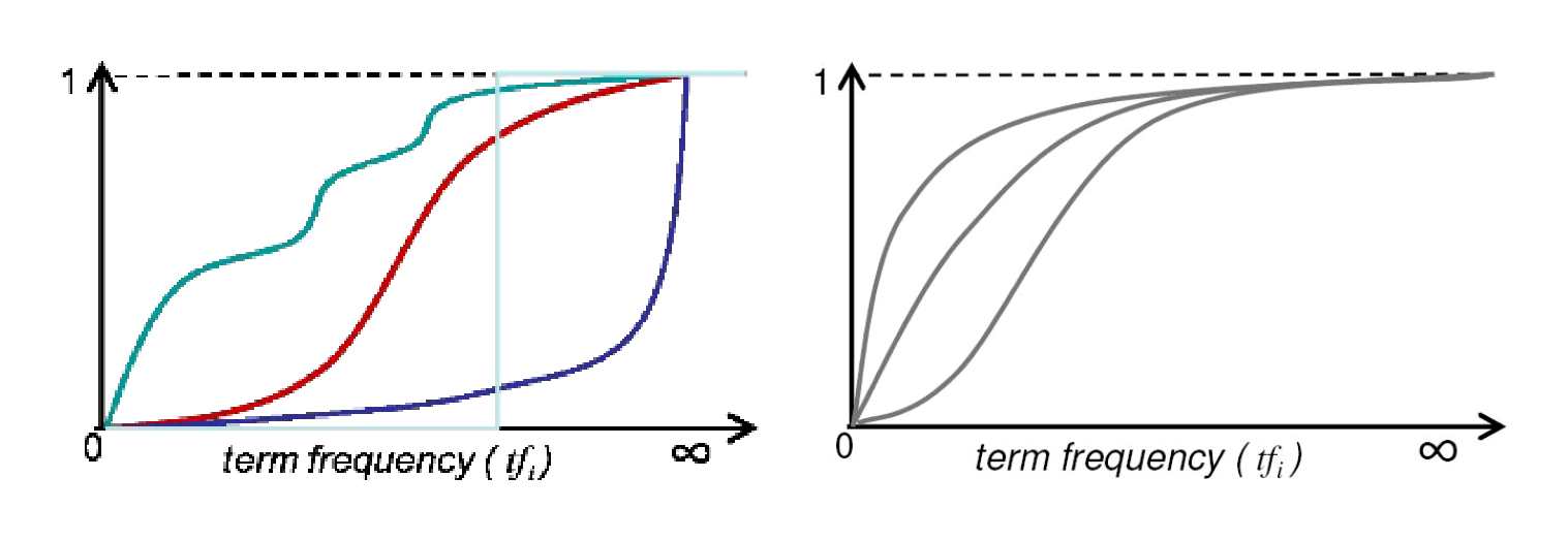
We investigate the shape of the saturation function a little more closely. It is clear that the properties listed above severely limit the possible functions; nevertheless, there remain many possibilities, as illustrated for example in the left-hand graph in Figure 3.2. However, the 2-Poisson model generates much smoother functions, as shown in the right-hand graph. For most realistic combinations of the parameters the curve is convex, as the top two lines; for some combinations it has an initial concavity, as the bottom line.

The next step in the development of BM25 is to approximate this shape. Lacking an appropriate generative corpus model from which to derive a convenient formula, the authors of BM25 decided to fit a simple parametric curve to this shape. The following one-parameter function was chosen:

$ \frac{tf}{k + tf} \quad \text{for some } k > 0 \tag{3.10} $

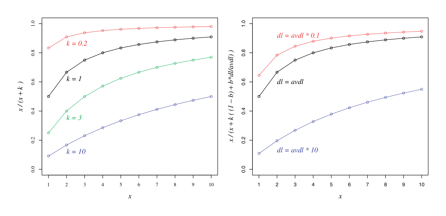
This function satisfies the properties listed above, and fits well the possible convex curves. We show values of this function for three different values of $k$ in Figure 3.3; the middle line is for $k = 1$, the upper line for lower $k$ and the lower line for higher $k$. Note that because we apply this to all terms, the absolute height does not matter; what matters is the relative increments for different increments in $tf$. Thus for high $k$, increments in $tf$ continue to contribute significantly to the score, whereas for low $k$, the additional contribution of a newly observed occurrence tails off very rapidly.

We obtain an early version of BM25 by combining the saturation function of Equation (3.10) with an approximation to the asymptotic maximum of Equation (3.9). The latter is obtained by using the old RSJ presence–absence term weight of Equation (3.2):

$ w_i(tf) = \frac{tf}{k + tf} w_i^{\text{RSJ}} \tag{3.11} $

(We will modify this below for the final version of BM25.)

The main thing missing so far from the analysis is the question of document length.

3.4.5 Document Length

The fixed-document-length assumption was made to allow a connection between a simple language model and BM25; we imagined an author filling a fixed number of slots with a fixed unigram model. Now we imagine instead that the author also chooses a document length.

We suppose that there is something like a standard length for a document, but that an author may decide to make a document longer or shorter; we consider only the longer case. Why might an author so decide? We can postulate two extreme cases:

Verbosity: Some authors are simply more verbose than others, using more words to say the same thing.
Scope: Some authors have more to say: they may write a single document containing or covering more ground. An extreme version would have the author writing two or more documents and concatenating them.

The verbosity hypothesis suggests that we should simply normalise any observed $tf$s by dividing by document length. The scope hypothesis, on the other hand, at least in its extreme version, suggests the opposite. In a real collection of documents we will observe variations in length, which might be due to either effect, or to a combination. We suppose in general a combination: that each hypothesis represents some partial explanation for the observed variation. This in turn suggests that we should apply some kind of soft normalisation.

We define document length in an obvious way:

document length: $dl := \sum_{i \in V} tf_i$

and also an average document length for the collection:

average doclength: $avdl$ (average over collection)

The length normalisation component will be defined in relation to the average; this ensures that the definition of document length used is not critical. In practice, we could take (for example) the number of characters in the document, or the number of words before parsing, or even the number of unique terms, and still get very similar results.

The soft length normalisation component is:

$ B := \left((1 - b) + b \frac{dl}{avdl}\right), \quad 0 \leq b \leq 1 \tag{3.12} $

Thus setting $b = 1$ will perform full document-length normalisation, while $b = 0$ will switch normalisation off. Now we use $B$ to normalise $tf$, before applying the saturation function, as follows:

$ tf' = \frac{tf}{B} \tag{3.13} $

$ w_i^{\text{BM25}}(tf) = \frac{tf'}{k_1 + tf'} w_i^{\text{RSJ}} \tag{3.14} $

$ = \frac{tf}{k_1 \left((1 - b) + b \frac{dl}{avdl}\right) + tf} w_i^{\text{RSJ}} \tag{3.15} $

This is the classic BM25 term-weighting and document-scoring function. As with all term-document weights defined in this survey, the full document score is obtained by summing these term-weights over the (original or expanded) set of query terms.

3.5 Uses of BM25

Section Summary: BM25 requires setting two internal parameters, b and k1, along with a relevance weighting component that functions like traditional inverse document frequency when no relevance judgments are available. This produces scores resembling tf-idf weighting, except that term frequency is moderated by a saturation effect that prevents scores from growing without limit. Experiments suggest reasonably effective parameter ranges, though results vary with document and query characteristics, and published implementations differ in minor ways such as handling of repeated query terms.

In order to use BM25 as a ranking function for retrieval, we need to choose values for the internal parameters $b$ and $k_1$, and also instantiate RSJ.

Concerning the RSJ weight (Equation (3.2)), all the previous comments apply. In particular, it can be used with or without relevance information. In the absence of relevance information, it reduces as before to a form of $idf$. In this case, the BM25 weight looks very much like a traditional $tf * idf$ weight — a product of two components, one based on $tf$ and one on $idf$. However, there is one significant difference. The $tf$ component involves the saturation function discussed, and is therefore somewhat unlike most other $tf$ functions seen in the literature, where common choices are $tf$ itself and $(1 + \log tf)$. The latter has a somewhat similar shape curve, but does not have an asymptotic maximum — it goes to infinity, even if somewhat slower than $tf$ itself.

Concerning the internal parameters, the model provides no guidance on how these should be set. This may be regarded as a limitation of the model. However, it provides an opportunity for optimisation, given some evaluated set of queries and relevance judgements in the traditional retrieval experiment style. A significant number of such experiments have been done, and suggest that in general values such as $0.5 < b < 0.8$ and $1.2 < k_1 < 2$ are reasonably good in many circumstances. However, there is also evidence that optimal values do depend on other factors (such as the type of documents or queries).

3.5.1 Some Variations on BM25

Published versions of BM25 can vary somewhat (the original BM25 [46] was a little more complicated than that of Equation (3.15), for example). Here we indicate some differences that might be encountered in different versions of the function in published sources.

• The original had a component for within-query term frequency $qtf$, for longer queries where a term might occur multiple times. In its full generality, this had a similar saturation function to that used for $tf$, but with its own $k_3$ constant. However, experiments suggested that the saturation effect for $qtf$ was unimportant, leading to a formula which was linear in $qtf$. In other words, one could simply treat multiple occurrences of a term in the query as different terms.
• The original also had a further correction for document length, to the total document score. This correction was again found to be unimportant.
• A common variant is to add a $(k_1 + 1)$ component to the numerator of the saturation function. This is the same for all terms, and therefore does not affect the ranking produced. The reason for including it was to make the final formula more compatible with the RSJ weight used on its own. If it is included, then a single occurrence of a term would have the same weight in both schemes.
• Some published versions are based on specific values assigned to $b$ and $k_1$. A common combination would be $b = 0.5$ and $k_1 = 2$. (However, many experiments suggest a somewhat lower value of $k_1$ and a somewhat higher value of $b$.)

3.6 Multiple Streams and BM25F

Section Summary: Documents in search systems are often divided into separate streams or fields, such as titles, bodies, or incoming anchor text, rather than treated as single unstructured blocks. BM25F extends the basic BM25 algorithm to handle these by assigning different weights and length normalizations to each stream when accumulating term frequencies, so that a match in a more predictive stream like a title contributes stronger evidence of relevance. The approach first pools evidence per term across streams before combining terms into an overall document score, allowing stream-specific adjustments for factors like verbosity while preserving the core saturation effect.

So far, all the arguments in this survey have been based on the idea that the document is a single body of text, unstructured and undifferentiated in any way. However, it is commonplace in search systems to assume at least some minimal structure to documents. In this section we consider documents which are structured into a set of fields or streams. The assumption is that there is a single flat stream structure, common to all documents. That is, there is a global set of labelled streams, and the text of each document is split between these streams. An obvious example is a title/abstract/body structure such as one might see in scientific papers. In the Web context, with extensive hyperlinks, it is usual to enhance the original texts with the anchor text of incoming links.

This is clearly a very minimal kind of structure; one can imagine many document structures that do not fit into this framework. Nevertheless, such minimal structures have proved useful in search. The general idea, not at all confined to the present framework but implemented in many different ways in different systems, is that some streams may be more predictive of relevance than others. In the above examples, a query match on the title might be expected to provide stronger evidence of possible relevance than an equivalent match on the body text. It is now well known in the Web context that matching on anchor text is a very strong signal.

3.6.1 Basic Idea

Given a ranking algorithm or function that can be applied to a piece of undifferentiated text, an obvious practical approach to such a stream structure would be to apply the function separately to each stream, and then combine these in some linear combination (with stream weights) for the final document score. In terms of the eliteness model, this approach may be regarded as assuming a separate eliteness property for each term/stream pair. Thus for a given term, eliteness in title would be assumed to be a different property from eliteness in body. Actually, the assumption would be even stronger: we would have to apply the usual assumptions of independence (given relevance) between these distinct eliteness properties for the same term.

This seems a little unreasonable—a better assumption might be that eliteness is a term/document property, shared across the streams of the document. We would then postulate that the relationship of eliteness to term frequency is stream-specific. In terms of the underlying language model discussed above, we might imagine that the author chooses a length for (say) the title and another for the body. Then, given eliteness (from the author’s choice of topics to cover), the unigram probabilities for the language model for filling the term-positions would also be stream-specific. In particular, there would be a much stronger bias to the elite terms when choosing words for the title than for the body (we expect a title to be much denser in topic-specific terms than an average body sentence).

The consequence of this term-document eliteness property is that we should combine evidence across terms and streams in the opposite order to that suggested above: first streams, then terms. That is, for each term, we should accumulate evidence for eliteness across all the streams. The saturation function should be applied at this stage, to the total evidence for each term. Then the final document score should be derived by combination across the terms.

3.6.2 Notation

We have a set of $S$ streams, and we wish to assign relative weights $v_s$ to them. For a given document, each stream has its associated length (the total length of the document would normally be the sum of the stream lengths). Each term in the document may occur in any of the streams, with any frequency; the total across streams of these term–stream frequencies would be the usual term-document frequency. The entire document becomes a vector of vectors.

streams: $s = 1, \dots, S$
stream lengths: $sl_s$
stream weights: $v_s$
document: $(\mathbf{tf}1, \dots, \mathbf{tf}{|V|})$ vector of vectors
$\mathbf{tf}i$ vector: $(tf{1i}, \dots, tf_{Si})$

where $tf_{si}$ is the frequency of term $i$ in stream $s$.

3.6.3 BM25F

The simplest extension of BM25 to weighted streams is to calculate a weighted variant of the total term frequency. This also implies having a similarly weighted variant of the total document length:

$ \tilde{tf}i = \sum{s=1}^S v_s tf_{si} \tag{3.16} $

$ \tilde{dl} = \sum_{s=1}^S v_s sl_s \tag{3.17} $

$av\tilde{dl}$ = average of $\tilde{dl}$ across documents

$ w_i^{\text{simpleBM25F}} = \frac{\tilde{tf}_i}{k_1 \left((1 - b) + b \frac{\tilde{dl}}{av\tilde{dl}}\right) + \tilde{tf}_i} w_i^{\text{RSJ}} \tag{3.18} $

However, we may also want to allow the parameters of BM25 to vary between streams — it may be that the different streams have different characteristics, e.g., in relation to verbosity v. scope (as defined in Section 3.4.5). It is in fact possible to re-arrange formula (3.15) so as to include any of the following in the stream-specific part: $k_1$, $b$, $w_i^{\text{RSJ}}$ or its non-feedback version $w_i^{\text{IDF}}$. We have in particular found it useful to allow $b$ to be stream-specific; we present here the appropriate version of BM25F:

$ \tilde{tf}i = \sum{s=1}^S v_s \frac{tf_{si}}{B_s} \tag{3.19} $

$ B_s = \left((1 - b_s) + b_s \frac{sl_s}{avsl_s}\right), \quad 0 \leq b_s \leq 1 \tag{3.20} $

$ w_i^{\text{BM25F}} = \frac{\tilde{tf}_i}{k_1 + \tilde{tf}_i} w_i^{\text{RSJ}} \tag{3.21} $

This version was used in [62]; the simple version in [50]. As usual, in the absence of relevance feedback information, $w_i^{\text{RSJ}}$ should be replaced by $w_i^{\text{IDF}}$. In [50, 62] we computed IDFs on the entire collection disregarding streams. This worked well in practice, but it can lead to degenerate cases (e.g., when a stream is extremely verbose and contains most terms for most documents). The proper definition of IDF in this context requires further research (this is also discussed in [37] where the notion of an expected idf is introduced).

As an illustration, we report in Table 3.1 the BM25F weights reported in [62] for the 2003 TREC Web Search tasks.

: Table 3.1. BM25F parameters reported in [62] for topic distillation (TD) and name page (NP) search tasks

\begin{tabular}{lrr}
\hline
Parameter & TD’03 & NP’03 \\
\hline
$k_1$ & 27.5 & 4.9 \\
$b_{title}$ & 0.95 & 0.6 \\
$b_{body}$ & 0.7 & 0.5 \\
$b_{anchor}$ & 0.6 & 0.6 \\
$v_{title}$ & 38.4 & 13.5 \\
$v_{body}$ & 1.0 & 1.0 \\
$v_{anchor}$ & 35 & 11.5 \\
\hline
\end{tabular}

3.6.4 Interpretation of the Simple Version

It is worth mentioning a very transparent interpretation of the simple version — although it does not apply directly to the version with variable $b$, it may give some insight. If the stream weights $v_s$ are integers, then we can see the simple BM25F formula as an ordinary BM25 function applied to a document in which some of the streams have been replicated. For example, if the streams and weights are ${v_{title} = 5, v_{abstract} = 2, v_{body} = 1}$, then formula 3.18 is equivalent to 3.15 applied to a document in which the title has been replicated five times and the abstract twice.

3.7 Non-Textual Relevance Features

Section Summary: The non-textual features of a document, such as its age, file type, or number of incoming links, can supply useful signals about its relevance that go beyond the words in the text. Under simple independence assumptions, these features can be folded directly into the usual BM25 scoring formula by adding a few extra weighted terms that depend only on the feature values themselves. Different smooth functions, such as a logarithm or a sigmoid, can be chosen to map each feature into a relevance weight, which in turn explains why ad-hoc combinations like BM25 plus PageRank often work well and how they can be refined.

In many collections there are other sources of relevance information besides the text. Things like the age of a file, its type or its link in-degree may provide useful information about the relevance of a document. The development of the PRF is quite general and does not make explicit reference to terms or text; it is therefore possible, at least in principle, to take non-textual features into account.

We will make two assumptions here about non-textual features. First we make the usual assumption of feature independence with respect to relevance odds (as discussed in Section 2). Second, we will assume that all non-textual features provide relevance information which is independent of the query. With these two assumptions we can integrate non-textual features very easily into the PRF and BM25 scoring frameworks. It is possible in principle to relax these assumptions and derive more sophisticated models of relevance for non-textual features.

Let us call $\mathbf{c} = (tf_1, \dots, tf_{|V|})$ the vector of term frequency counts of document $d$, and let us call $\mathbf{f}$ an extra vector of non-textual features $\mathbf{f} = (f_1, \dots, f_F)$. We have that $d = (\mathbf{c}, \mathbf{f})$.

Note that the initial PRF development (Equations (2.1–2.4) in Section 2) applies also to this extended version of $d$. Equation (2.4) makes the assumption of feature independence, which carries over the non-textual features. Therefore the product in Equation 2.4 would include all non-textual features $\mathbf{f}$.

In Equation (2.5), where we drop all the non-query terms in $\mathbf{c}$, none of the terms in $\mathbf{f}$ would be dropped — non-textual features are assumed to be correlated with relevance for all queries. After taking the log in Equation (2.6) we see that the addition of non-textual features simply adds a new term to the sum. Removing the zeros in Equations (2.7–2.9) does not affect this term, so after (2.11) we may write:

$ P(rel|d,q) \propto_q \sum_{q,tf_i>0} W_i(tf_i) + \sum_{i=1}^F \lambda_i V_i(f_i), \tag{3.22} $

where

$ V_i(f_i) := \log \frac{P(F_i = f_i | rel)}{P(F_i = f_i | \overline{rel})} \tag{3.23} $

We have artificially added a free parameter $\lambda_i$ to account for rescalings in the approximation of $W_i$ and $V_i$.

We note that features $f_i$ may well be multi-valued or continuous, and this implies the need for care in the choice of function $V(f_i)$ (just as we paid attention to finding a good function of $tf$). This will depend on the nature of each non-textual feature $f_i$ and our prior knowledge about it. Here are some $V_i$ functions that we have used with success in the past for different features:

• Logarithmic: $\log(\lambda'_i + f_i)$
• Rational: $f_i / (\lambda'_i + f_i)$
• Sigmoid: $[\lambda'_i + \exp(-f_i \lambda''_i)]^{-1}$

This development can explain for example why simple scoring functions such as $\text{BM25F}(q, d) + \log(PageRank(d))$ may work well in practice for Web Search retrieval. This can much improved by adding the scaling parameter $\lambda$, and it can be further improved (only slightly) by changing the log into a sigmoid and tuning the two extra parameters $\lambda'$ and $\lambda''$ [12]. In our work we developed more sophisticated ranking functions integrating several forms of non-textual information and using over a dozen parameters [12, 13]. The optimisation of these parameters is discussed in Section 5.

3.8 Positional Information

Section Summary: The probabilistic retrieval framework largely overlooks where query terms appear in a document and instead focuses only on how often they occur. Modeling relevance with positional details has proven difficult, as it leads to overly complex event spaces and parameter counts, while experiments have consistently shown only modest gains in accuracy. Proposed workarounds such as indexing phrases, scoring passages, or adding proximity features do not integrate naturally into the framework, and the robustness of natural language may explain why term positions are often less critical than they first appear.

For the most part the PRF ignores positional information: it cares only about the number of occurrences of a term, but not about their position. There are two important reasons that have held back the PRF from considering positional information: (i) it is extremely hard to develop a sound formal model of relevance which takes into account positional information without exploding the number of parameters, and (ii) position information has been shown to have surprisingly little effect on retrieval accuracy on average. In this section we only give an overview of the existing approaches and discuss the main difficulties. We also propose some intuitions of why position may not be as crucial as it seems at first sight.

Why is it so hard to model relevance with respect to the position of terms in the query and document? Several problems appear. First, we need to define an appropriate universe of events. In the traditional PRF this universe is simply $\mathbb{N}^{|q|}$, all possible term frequency vectors of terms in the query. The most natural way to consider positions would be to characterise all sequences of terms in the query separated by some number of non-query terms. This leads to an excessively high-dimensional space, and one that is very hard to factor it in an appropriate way. In the traditional model the natural unit over which we build (factorise) the required quantities is the occurrence of a term a given number of times. What would be the natural unit over which we build (factorise) the probabilities required to model positions adequately?

There have been a number of attempts to deal with these issues and introduce positional information into BM25 (see for example [3, 54, 51] and references therein). The three main approaches used are the following:

1. Indexing phrases as individual terms. This approach is ideal for multi-term tokens (such as White House) for which a partial match would in fact be incorrect. Its implementation is extremely simple since one does not need to modify the ranking function in any way (each phrase would have its own $tf$ and $idf$). There are three problems however: (i) it does not take into account partial matches; (ii) it does not take into account terms which are close but not exactly adjacent; and (iii) one needs to define the valid phrases [48].
2. Scoring spans of text instead of entire documents. This can be done explicitly, with a passage retrieval ranking function [3], or implicitly by constructing a ranking function that integrates scores computed over many document spans [51].
3. Deriving position features (such as the minimum and maximum length of the document spans containing all the terms in the query) which can then be integrated into the scoring function as non-textual features (as those in Section 3.7) [54].

In our opinion none of these attempts would qualify as a natural extension of the PRF, since it is not clear what the assumptions about relevance are. Metzler [32, 33] proposes a novel probabilistic retrieval model which makes clear assumptions about positions and relevance, and could perhaps be integrated within the PRF. The model estimates the probability of relevance of document and query jointly: $P(Q, D | Rel)$. This is done by a Markov Random Field (MRF) which can take into account term-positions in a natural way. The MRF can use any appropriately defined potentials: while the original work used LM-derived potentials, BM25-like potentials were used in [31]. However, even when using BM25-like potentials, we cannot call this model an extension of the PRF, since it models a different distribution: $P(D, Q | Rel)$ instead of the posterior $P(Rel | D, Q)$.

We end this section with a brief discussion of why position information may not be as important as it may seem at first view. It is sobering to see how hard it has been in the past to effectively use proximity in IR experiments. All the works referenced in this section claim statistically significant improvements over non-positional baselines, but the improvements reported are small. We believe this is specially the case for small collections and high recall situations (typical of academic IR evaluations), since position information is a precision enhancement technique. But even in large collections with high-precision requirements (such as realistic Web Search evaluations) the gains observed are small. Why is this? We do not know of theoretical or empirical studies about this, but we propose here two hypotheses.

First, we believe that natural language, and queries in particular, are quite robust. We would argue that for many queries, a human could determine the relevance of a document to a query even after words in the document and query were scrambled. And for cases that this is not true, it is likely that the user would unconsciously correct the query by adding terms to it that disambiguate it. This does not mean that all queries and documents are position-proof, but the fraction that require positions is small. Second, it should be noted that taking into account the structure of a document (e.g., in BM25F) implicitly rewards proximity within important short streams, such as the title.

3.9 Open Source Implementations of BM25 and BM25F

Section Summary: Several open-source search engines implement the BM25 ranking method, though only MG4J provides full support for its field-weighted version known as BM25F. Systems such as Lemur, Terrier, Xapian, and others handle BM25, while Lucene relies on third-party extensions for both approaches. After reviewing the code, the authors consider the implementations correct overall, aside from minor variations, but note that none include built-in tools for automatically tuning the model's parameters.

We review here several implementations of BM25 and BM25F available as open source. This list is not exhaustive, there may be other search engines or extensions of them that implement BM25 and BM25F.

As far as we know only the MG4J [9, 34] fully implements BM25F (version 2.2 or later). BM25 is implemented by Lemur, MG4J, Okapi, PF/Tijah, Terrier, Wumpus, Xapian and Zettair [22, 27, 34, 35, 39, 56, 57, 60, 61, 63]. All these search engines are quite modular and could in principle be modified to extend BM25 in a number of ways, in particular to implement BM25F. Lucene [29] does not implement BM25 but there exist a third party Lucene extensions that implement BM25 and BM25F [38]. We inspected the code of all these implementations and we believe they are correct.[^1] (inspection was visual: we did not run tests ourselves; in two cases implementation was incorrect and we asked the authors to correct it, which they did). None of the systems above provide support for parameter optimisation, although it should not be difficult to extend them for this.

[^1]: There are some minor differences in BM25 implementations in these packages at the time of writing this survey. For example, PF/Tijah uses $idf = \log \frac{N+0.5}{n+0.5}$, Terrier does not allow modifying $k$ programmatically and Xapian does not allow modifying any parameters programmatically.

4 Comparison with Other Models

The first probabilistic model for retrieval was proposed by Maron and Kuhns in 1960 [30]. It was similarly based on a notion of probability of relevance; however, there was an interesting discrepancy between the Maron and Kuhns approach and that of Robertson and Spärck Jones fifteen years later. The discrepancy was the subject of research in the early 1980s on a unification of the two. In order to explain both the discrepancy and the attempted unification, we first describe the Maron and Kuhns model.

4.1 Maron and Kuhns

Section Summary: Maron and Kuhns described indexing as a process in which a librarian assigns subject headings to a book by estimating, for each heading, the chance that users who search under it will find the book useful. Their approach therefore treats the probability of relevance as a proportion of users with similar needs rather than as a property of the document alone. The authors note that today’s large-scale click logs from repeated web queries resemble this kind of user-centered evidence, though the precise link to formal retrieval models still requires clarification.

The situation envisaged by Maron and Kuhns was that of a librarian indexing a book (document). The idea was that indexing should anticipate how people make requests in the first place. Ideal indexing should match the requests of just those people who would want to be pointed to this monograph — those people who would find it relevant to their needs. The system was assumed to be a system of subject headings, any of which might be assigned by the librarian to the book in question; a user request would take the form of a chosen subject heading to look under. Thus the librarian would be invited to estimate, in respect of each candidate subject heading, the probability that a user looking there would find this particular book relevant.

Thus far, the basis for the model looks very like the PRF defined in Section 2. However, to better understand the nature of the probability of relevance as interpreted by Maron and Kuhns, we need to consider the event space in which it is defined. This will give us the basis for a comparison in the following section.

We have (at least in the mind of the librarian) a group of users (with information needs) who look under a particular subject heading. On the other hand, we have a single individual book in front of the librarian. Therefore the event space involved, in which the probability should be defined, is a space of users. If we were to attempt to use feedback to estimate such a probability, we would ideally count users — that is, of all the users who express their queries by means of a particular subject heading, what proportion would like this monograph.

This kind of approach has recently acquired new force, because the big Web Search engines typically see some queries (the so-called ‘head’ queries) repeated very many times by different users. Click log data looks a little like relevance feedback on individual documents from a population of users with similar queries. However, the relation between this and the PRF discussed in this monograph needs further analysis.

4.2 The Unified Model

Section Summary: The unified model tries to combine two different ways of estimating the probability that a document is relevant to a user by imagining a matrix of individual users against individual documents. It defines four related probabilities, starting with a general estimate based on groups of similar users and similar documents, then refining that estimate with feedback on a specific document, a specific user, or both. Although this approach can draw on richer sources of evidence such as logged web searches, it still cannot directly assign a probability to one exact user–document pair without observing that pair itself.

We re-visit the original RSJ model, the foundation of the model presented in this survey, in order to define it in similar terms. In this case, we start with a single individual user, who puts a request using certain words. Now we ask the question, what is the probability that any arbitrary document matching one (or a combination) of these words is relevant to the user. Thus the event space here consists of documents, and if we want to use feedback to estimate the probability, we would count documents, as in Section 3.1.

It immediately becomes clear that although both models refer to probability of relevance, they define their respective versions of this probability in different event spaces. In fact, the two probabilities of relevance are actually quite distinct.

The unification attempt [43] was based on the following argument. We imagine a matrix of users-with-information-needs against documents (individual users $u$, individual documents $d$). Ideally we would like to assign a meaningful probability of relevance to the specific combination of an individual user with an individual document: $P(rel|u, d)$. However, doing this directly looks difficult — at least if we are looking for direct evidence (feedback). If we show $d$ to $u$ and get a judgement, we no longer need to assign a probability! Indeed, it only makes sense to do so when we have classes of similar events.

Maron and Kuhns start by classifying users together, according to the subject headings they consult. Thus we are dealing with a class $U$ of users, and ask about $P(rel|U, d)$. On the other hand, Robertson and Spärck Jones classify documents together in classes such as $D$, and ask about $P(rel|u, D)$.

The unified model proceeded to define four different probabilities of relevance. We might consider starting with $P(rel|U, D)$, which is a general model needing only feedback from similar users about similar documents (this is referred to as Model 0). If we have feedback about the particular document, we can improve this estimate by considering $P(rel|U, d)$ (Model 1). On the other hand, if we have feedback from the particular user, we should go for $P(rel|u, D)$ (Model 2). Finally, if we have both kinds of more specialist evidence simultaneously (Model 3), we might aim for an even better probability. However, its exact relationship to $P(rel|u, d)$ is not quite obvious, because while it is based on feedback of the above three kinds, it would not actually have feedback on the exact individual pair.

The unified model has been the subject of some more recent work [8], and we are now entering a domain in which many different kinds of feedback may be possible, given the kind of logging of Web searching behaviour that is now the norm. Other authors (for example [14, 17], and later [25] in the context of the language model discussed below) have approached the problem by in effect limiting themselves to Model 0, by considering only representations of documents and queries, rather than individual instances.

4.3 The Simple Language Model

Section Summary: The simple language model treats any text as the output of a statistical process that generates words one by one according to fixed probabilities drawn from a vocabulary. In retrieval, each document is given its own such model, and documents are ranked by the probability that the user’s query would have been produced by that same model; relevance is therefore understood only as a match between the query text and the document’s underlying word distribution. To keep probabilities from dropping to zero for unseen words, the document model is smoothed by mixing its own term frequencies with those from a general background collection.

The language model (LM) of IR is a more recent innovation [24, 26, 33], also with a strong probabilistic motivation. We first describe the simple LM, and then some more sophisticated developments.

In the LM, we regard any piece of text (document, query, etc.) as having been generated by a statistical process. Outside of IR, such models have been very successful in various areas, particularly in speech recognition, and the IR application has borrowed from that domain. In this particular view of text, it is regarded as being generated word-by-word in sequence, each word being chosen from a vocabulary. The simplest statistical model, so-called unigram, has a fixed probability distribution over the vocabulary, applied to all word-positions (so actually the sequence is not important). $n$-gram models assume that the choice of the next word depends on the $n - 1$ previous words chosen.

The simple LM approach to IR assumes that each document has its own model, and asks this question about each document: what is the probability that the query came from (was generated by) the same language model as the document (there is no separate query model in this approach). This probability is used to rank documents for a query. Thus there is no explicit notion of relevance; the implicit notion is that a document is relevant to a query if the query came from the same language model as the document. This approach also does not distinguish between individual users — a query is understood to be just a text, and each query–document pair is considered as an equivalent individual event. From an individual user point of view, the model implicitly assumes that there is just one relevant document (if this instance of a query was generated by the language model for document 1, it could not also have been generated by the different language model for document 2). However, since the approach does not distinguish individuals, in effect it represents a version of Model 0 (in the terms of the unified model, as discussed above). Different instances of the same query can be generated from different documents; in the $(U, D)$ class, more than one document can be relevant. But it follows that it makes no sense to consider individual feedback in the context of the simple LM.

In more detail, the document language model is usually built by mixing (smoothing) probabilities derived from the document itself with those taken from a general background language model. One purpose of this smoothing is to avoid a zero probability being assigned to any term that does not occur in the document. In general, a rich fund of models and estimation methods has been mined within the general framework of the LM. We further explore only two of these developments in the following sections.

4.4 The Relevance (Language) Model

Section Summary: The relevance model improves on basic language modeling by treating the query itself as the source of a distinct statistical distribution over words, which can be refined with user feedback on relevant documents. Unlike earlier approaches where matching rules were built directly into the model, this framework requires selecting an external method to compare the query distribution against each document's word distribution. The standard choice for that comparison is the Kullback-Leibler divergence measure, which has shown strong performance in practice.

Some of the limitations of the simple model are addressed in work on a relevance model for the LM framework [26, 33]. Here, by contrast, we assume that the query has (that is, is generated by) its own model, distinct from any particular document model. The initial source for this model is clearly the query itself; however, relevance feedback (from the individual user, for example) can provide additional evidence about it.

With this approach, the document–query matching process becomes much less obvious. Note that both in the simple LM, and in the traditional probabilistic relevance framework (PRF) described in this survey, the process of matching the query to the document is inherent in the model, entirely determined by the model itself. In this new context, no such matching process is defined; it is necessary to choose one from outside the model.

Given that both the document LM and the query (relevance) LM take the form of statistical distributions over a vocabulary, matching becomes a question of matching two statistical distributions. The most common way to do this is to use the Kullback–Leibler (KL) divergence measure. This has good empirical support.

4.5 Topic Models

Section Summary: Researchers have explored implicit topic models, such as latent semantic indexing and latent Dirichlet allocation, which uncover hidden themes in the statistical patterns of document language as one possible link between language modeling and probabilistic relevance frameworks. These models bear some resemblance to the single eliteness variable per term in the relevance framework and to parsimonious language models that differentiate a document from background text. Even so, the field remains far from any true unification of the two approaches.

There is perhaps potential for some kind of bridge between the LM approach and the PRF in work on implicit topic models. Most such work has sought to discover the topics implicit in the statistical structure of the language of documents; examples are Latent Semantic Indexing (LSI) [18], Probabilistic LSI [21] and Latent Dirichlet Allocation [7]. The hidden eliteness variables postulated in the probabilistic relevance framework have some similarities (although much simplified by the assumption of one eliteness variable per term). A related approach is the parsimonious LM [20], which attempts to model in what ways a particular document or query is distinguished from the general background language. However, we appear to be some distance from a serious unification of the LM and the PRF which is the main subject of this survey.

4.6 Divergence from Randomness

Section Summary: Divergence from randomness models evaluate documents by examining how the distribution of terms deviates from what would be expected by chance alone, treating such deviations as an implicit indicator of relevance. Like language modeling approaches, these methods avoid using relevance as a basic concept and instead focus purely on statistical patterns in the collection. A range of term-weighting schemes and ranking formulas can be derived within this framework, some of which closely resemble the well-known BM25 function.

The DFR models [2], like the language models, do not contain “relevance” as a primitive notion. Also like the language models, they concentrate on the statistical distribution of terms in documents. In general, they seek to identify the ways in which term distributions differ from what one might expect on a random basis — evidence of such divergence is taken implicitly as evidence about relevance.

It is possible to derive a variety of term-weighting and document ranking functions within this framework, including a formulation that is approximately the same as BM25.

5 Parameter Optimisation

Like most IR models, the models in the PRF have free parameters that need to be set to appropriate values. The BM25 and BM25F models are known to be quite robust with respect to their parameters, meaning that small changes in the parameter values (or in the collection) do not produce large changes in accuracy or relevance. Nevertheless significant gains in relevance can be obtained by properly optimising the parameters, specially when we deal with a new collection.

Parameter optimisation comes with considerable costs: it will require the human evaluation of many query results, which is expensive, and the optimised parameters will be specific to the collection evaluated and may not work well for other collections. Furthermore, the optimisation procedure can be computationally costly, requiring more computing power that the search engine itself. For these reasons this approach is only appropriate for specific collections which merit the cost needed to optimise the ranking function. Examples of such collections are the WWW, large corporate collections or high-value News or Help sites.

Let us call $\theta$ the vector of all free parameters of the ranking model being tuned. In the case of BM25 this vector would have two components: $\theta = (k_1, b)$. In the case of BM25F it would have more: $\theta = (k_1, b_1, \dots, b_S, v_1, \dots, v_S)$. If we include non-textual features then we have even more parameters, the exact number depending on the transformation used for each non-textual feature.

‘Tuning’ the parameters of the model can be seen as an optimisation problem, where we seek to maximise the relevance of the ranking model with respect to the model parameters $\theta$, for a given set of relevance judgements. More specifically, if we fix the document collection and a set of queries with their associated relevance judgements, then for any parameter setting $\theta$ we can compute the performance measure of our choice $M(\theta)$. What is left is to find the parameter setting that maximises $M(\theta)$. This is exactly an $n$-dimensional optimisation problem with $M$ as the target function being optimised over the space of valid $\theta$ values.

Optimising standard IR measures,[^1] however, is not easy: they are very expensive to evaluate, they have local maxima and plateaus, they are not smooth and they don’t have gradients [49]. For these reasons, it is not easy to apply standard optimisation techniques. Even applying simple 0-th order optimisation techniques such as trusted region optimisation is difficult and expensive. In practice we use a number of ad hoc techniques to speed up exhaustive search. We will discuss these in the next subsection.

[^1]: Such as Average Precision, Precision@k, Mean Reciprocal Rank and Discounted Cumulative Gain.

Another alternative is to change the function being optimised. This approach is specially useful when one is optimising very many features, and is discussed in the last subsection.

5.1 Greedy Optimisation

Section Summary: The section describes practical techniques for efficiently searching large spaces of model parameters when each evaluation is costly. It explains the use of caching to avoid repeating evaluations, combined with a minimum-resolution grid on parameter values that improves cache hit rates and speeds convergence without harming performance. It also presents a robust line search procedure that repeatedly evaluates a one-dimensional interval, then recenters and rescales the interval around the best point found so far until the desired precision is reached.

We discuss here a number of techniques (some heuristics, some implementation tricks) we used in the past to speedup the exhaustive search and find good parameter values.

Caching: Because function evaluations are so expensive, we cache the evaluations. Indeed we may often re-visit a parameter value in our search for the optimum. It would be wasteful to re-evaluate all the queries; instead, we store the resulting relevance in a hash table using the parameter values as the key: $H[\theta] \leftarrow M(\theta)$.

Grid: It is also useful to set a minimum resolution for every parameter, defining a grid of allowed parameters values. For example, in most of our experiments we did not allow parameters to change beyond the second decimal. This has negligible affect on the relevance performance and greatly increases the effect of caching and the speed of convergence. Furthermore it makes it easier to report and share parameter values.

5.1.1 Robust Line Search

We first consider methods for optimising over a single parameter. Most parameters being optimised are positive but unbounded above. Therefore we do not know the region of interest of the parameter being optimised, nor do we know the required resolution (the size of the intervals to be tested). For this reason we developed the following search algorithm, which we call Robust Line Search (RLS).

Call $l$ and $r$ the current left and right brackets of the $1-\text{D}$ search space. Split the region in $m$ equal parts of size $(r - l)/m$. Compute the performance on the $m + 1$ region boundaries, and call $c$ the boundary with the highest performance.

The idea is to move towards $c$ by re-centering the search region around $c$ and scaling it appropriately. If $l < c < r$ we need to zoom in into $c$, by scaling down the search region. Since the function being optimised has local maxima we cannot zoom too much, or we may completely lose the global maximum; for this reason we tend to zoom very conservatively. On the other hand, if $c$ equals $r$ or $l$, it is most likely that the maximum is outside the current search region, and possibly far away. Therefore we increase the size of the search region. We iterate this until $l$ and $r$ are within the some minimum distance, typically below the minimum resolution set. An example optimisation is illustrated in Figure 5.1.

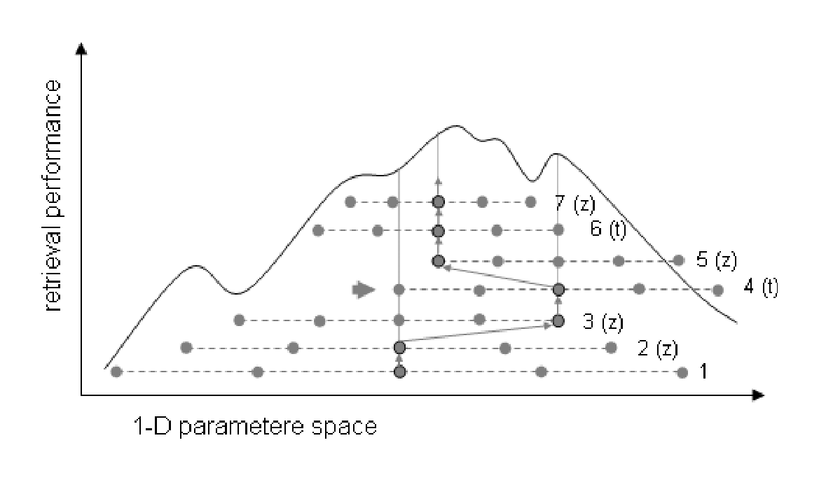
5.2 Multidimensional Optimisation

Section Summary: Multidimensional optimization extends one-dimensional methods to multiple parameters through two practical strategies. The greedy robust line search recursively optimizes each primary parameter while treating the rest as subordinate variables that must themselves be locally optimized, but the approach scales exponentially and becomes impractical beyond a handful of dimensions. A more efficient alternative, called promising directions, independently optimizes each parameter from an initial point, then performs one additional search along the vector connecting the starting and optimized values before repeating; this costs only linearly in the number of dimensions and can be further accelerated by factoring the work into sequential batches of interdependent parameters, such as tuning BM25F stream weights and length-normalization factors in a fixed schedule.

Any 1-D optimisation method can be generalised to $n\text{-D}$ in several ways. We have used two methods to do this, both of which worked well in practice.

Greedy Robust Line Search: Imagine that we want to run the RLS method on a 2-D problem, with parameters $\theta = (\theta_1, \theta_2)$. Let’s leave $\theta_2$ as a subordinate variable and run RLS on $\theta_1$. Every time that we need to compute the performance $M(\theta)$ at a given point $\theta_1 = z$, we would need to fix the subordinate $\theta_2$ at its optimal value. To find out this value, we can run a local RLS to optimise $\theta_2$ locally while keeping $\theta_1 = z$. Generalising this, every line optimisation with $i$ parameters fires off an optimisation with $i - 1$ subordinate parameters and so on, recursively. Of course this is a greedy approximation to the exhaustive (exponential) exploration of the parameter space, because we are running RLS. However, this approach remains exponentially expensive with respect to $n$ because of its recursive nature, and therefore it is not practicable for large $n$ (e.g., $n > 3$).

Promising Directions: Another way we have used to carry out searches in $n$ dimensions is the following.[^2] Choose an initial point for each parameter (call the resulting the vector $\theta$). Run $n$ $1-\text{D}$ independent searches, to find the optimum value $\theta'_i$ of each parameter when all others are kept fixed at $\theta$. Each of these optimal values found defines a promising directions in parameter space. Now consider the vector going from $\theta$ to $\theta' = (\theta'_1, \dots, \theta'_n)$. We expect this vector to move through interesting regions of space if there is correlation between features. Therefore we do one more $1-\text{D}$ optimisation along this line. We do this by re-parameterising the system with a new variable that moves all parameters linearly from $\theta$ to $\theta'$. Finally we choose the best parameter setting found so far and we re-start the process. An example optimisation is illustrated in Figure 5.2, where we show the first two iterations (noted 1 and 2), each consisting of three line searches (noted a, b and c). The total cost of an iteration is $(n + 1)$ $1-\text{D}$ optimisations. Therefore, it grows only linearly with $n$, but it may require very many iterations to complete.

[^2]: This method can be seen as a linear version of trusted region optimisation methods [4, 5]; it has the advantage of requiring much fewer function evaluations, which are extremely expensive in our case.

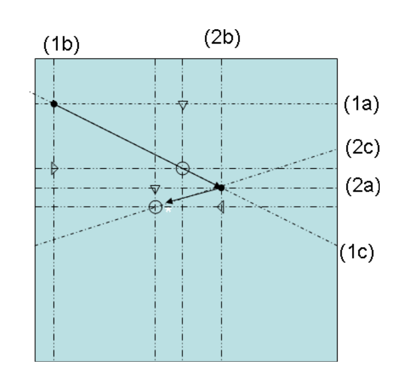
K1 Scaling: Note that in general $k_1$ will depend on the weights assigned to streams in BM25F, even if it is kept as a stream-independent parameter. This is because the stream weights in effect rescale the $tf$ values, and $k_1$ has to be adjusted accordingly. If we have a good $k_1^{\text{BM}25}$ value for the regular BM25 function (no streams), we can propose a good initial value of $k_1$ for BM25F by scaling it according to the change in average document length from the unweighted to the weighted form:

$ k_1^{\text{BM}25\text{F}} \approx k_1^{\text{BM}25} \frac{\sum_s v_s \text{avsl}_s}{\sum_s \text{avsl}_s} \tag{5.1} $

5.2.1 Factoring the Search

A very useful technique for speeding up the search in practice is to factor the search into batches, optimising together only the parameters that are known to be strongly dependent. When doing this it is important to choose the initial parameters and the order of the batches judiciously. A typical schedule for BM25F may be:

1. Compute the optimal $k_1$ and $b$ (ignoring streams). This is equivalent to setting all $v_s = 1$ and all $b_s = b$. (Cost: $1 \times 2\text{D}$);
2. Optimise stream weights ${v_s}_{s=1..S}$ jointly. We use here the $k_1$ re-scaling trick in Step (5.1). (Cost: $1 \times S\text{D}$); and
3. Optimise $k_1$ and ${b_s}_{s=1..S}$ independently (Cost: $(S + 1) \times 1\text{D}$).

This schedule may be repeated until no further increase in performance is obtained. When dealing with non-textual features, the optimisation above is usually interleaved with the optimisation of the non-textual features, which can also be done independently or jointly by batches.

5.3 Gradient Optimisation

Section Summary: Researchers have explored directly optimizing performance measures in information retrieval by using machine learning techniques based on gradient methods. The key step is to approximate complex ranking metrics such as NDCG with smoother functions whose gradients are known, allowing efficient adjustment of many parameters at once without exponential slowdown. This approach also supports joint tuning when BM25F is combined with large numbers of other features inside broader models such as neural networks.

A different possibility is to choose a performance function that can be optimised directly by machine learning techniques. This approach was pursued with some success a few years ago [1, 10, 55], and has now become an active area of research (see for example the recent NIPS and SIGIR workshops on this topic [23, 28]). The main idea is to approximate rank-dependant relevance functions such as NDCG by a function with known gradients. Then we can apply the battery of gradient-based optimisation methods. The speed of these methods does not grow exponentially with the number of dimensions optimised, so one can optimise very many parameters simultaneously. Furthermore, if BM25F is being combined with a larger number of other (non-textual) features, methods can be used to optimise jointly all parameters. For example, this is the case in [55] where the overall model is an artificial neural network which takes as input many features, one of them being BM25F. It is out of the scope of this survey to detail gradient-based optimisation methods.

6 Conclusions

The classical probabilistic relevance framework has provided a series of well-founded scoring formula, as well as some significant insights into different aspects of search. One of the reasons of the success of the PRF, we believe, is the powerful combination of sound theoretical modelling and a pragmatic parameterisation that exploits our prior knowledge in IR. We do not believe that the PRF has reached the end of its useful life. When it is well understood, the PRF model can provide a solid ground on which to analyse new IR problems and derive new solutions.

References

Section Summary: This section consists of a bibliography listing scholarly papers, books, workshop proceedings, and software project links centered on probabilistic approaches to information retrieval, document ranking, and related machine learning methods. The cited works span foundational research from the 1960s onward alongside more recent contributions from conferences such as SIGIR and TREC, often addressing models of relevance, language modeling, and optimization techniques. Several entries also reference toolkits and systems for implementing search and ranking functionality.

[1] S. Agarwal, C. Cortes, and R. Herbrich, eds., Proceedings of the NIPS 2005 Workshop on Learning to Rank, 2005.

[2] G. Amati, C. J. van Rijsbergen, and C. Joost, “Probabilistic models of information retrieval based on measuring the divergence from randomness,” ACM Transactions on Information Systems, vol. 20, no. 4, pp. 357–389, 2002.

[3] M. M. Beaulieu, M. Gatford, X. Huang, S. E. Robertson, S. Walker, and P. Williams, “Okapi at TREC-5,” The Fifth Text Retrieval Conference (TREC-5). NIST Special Publication 500-238, pp. 143–165, 1997.

[4] F. V. Berghen, “Trust Region Algorithms,” Webpage, http://www.lemurproject.org.

[5] F. V. Berghen, “CONDOR: A constrained, non-linear, derivative-free parallel optimizer for continuous, high computing load, noisy objective functions,” PhD thesis, Université Libre de Bruxelles, 2004.

[6] C. Bishop, Pattern Recognition and Machine Learning (Information Science and Statistics). Springer, 2006.

[7] D. M. Blei, A. Y. Ng, and M. I. Jordan, “Latent dirichlet allocation,” Journal of Machine Learning Research, vol. 3, pp. 993–1022, 2003.

[8] D. Bodoff and S. E. Robertson, “A new unified probabilistic model,” Journal of the American Society for Information Science and Technology, vol. 55, pp. 471–487, 2004.

[9] P. Boldi and S. Vigna, “MG4J at TREC 2005,” in The Fourteenth Text Retrieval Conference (TREC 2005) Proceedings, NIST Special Publication 500-266, 2005. http://mg4j.dsi.unimi.it/.

[10] C. Burges, T. Shaked, E. Renshaw, A. Lazier, M. Deeds, N. Hamilton, and G. Hullender, “Learning to rank using gradient descent,” in Proceedings of the International Conference on Machine Learning (ICML), vol. 22, p. 89, 2005.

[11] W. Cooper, “Some inconsistencies and misidentified modelling assumptions in probabilistic information retrieval,” ACM Transactions on Information Systems, vol. 13, pp. 110–111, 1995.

[12] N. Craswell, S. E. Robertson, H. Zaragoza, and M. Taylor, “Relevance weighting for query independent evidence,” in Proceedings of the 28th Annual International ACM SIGIR Conference on Research and Development in Information Retrieval, pp. 472–479, ACM, 2005.

[13] N. Craswell, H. Zaragoza, and S. E. Robertson, “Microsoft Cambridge at TREC-14: Enterprise track,” in The Fourteenth Text Retrieval Conference (TREC 2005), 2005.

[14] F. Crestani, M. Lalmas, C. J. van Rijsbergen, and I. Campbell, ““Is this document relevant? ... probably”: A survey of probabilistic models in information retrieval,” ACM Computing Surveys, vol. 30, no. 4, 1998.

[15] W. B. Croft and D. J. Harper, “Using probabilistic models of document retrieval without relevance information,” Journal of Documentation, vol. 35, pp. 285–295, 1979.

[16] W. Feller, An Introduction to Probability Theory and Its Applications, vol. 1. Wiley, 1968.

[17] N. Fuhr, “Probabilistic Models in Information Retrieval,” The Computer Journal, vol. 35, no. 3, 1992.

[18] G. W. Furnas, S. Deerwester, S. T. Dumais, T. K. Landauer, R. A. Harshman, L. A. Streeter, and K. E. Lochbaum, “Information retrieval using a singular value decomposition model of latent semantic structure,” in Proceedings of the 11th Annual International ACM SIGIR Conference on Research and Development in Information Retrieval, pp. 465–480, ACM, 1988.

[19] S. P. Harter, “A probabilistic approach to automatic keyword indexing (parts 1 and 2),” Journal of the American Society for Information Science, vol. 26, pp. 197–206 and 280–289, 1975.

[20] D. Hiemstra, S. E. Robertson, and H. Zaragoza, “Parsimonious language models for information retrieval,” in Proceedings of the 27th Annual International ACM SIGIR Conference on Research and Development in Information Retrieval, pp. 178–185, ACM, 2004.

[21] T. Hofmann, “Probabilistic latent semantic indexing,” in Proceedings of the 22nd Annual International ACM SIGIR Conference on Research and Development in Information Retrieval, pp. 50–57, ACM, 1999.

[22] Indri. Homepage. http://www.lemurproject.org/indri.

[23] T. Joachims, H. Li, T. Y. Liu, and C. Zhai, “Learning to rank for information retrieval (LR4IR 2007),” SIGIR Forum, vol. 41, no. 2, pp. 58–62, 2007.

[24] J. Lafferty and C. Zhai, “Document language models, query models, and risk minimization for information retrieval,” in Proceedings of the 24th Annual International ACM SIGIR Conference on Research and Development in Information Retrieval, ACM, 2001.

[25] J. Lafferty and C. Zhai, “Probabilistic relevance models based on document and query generation,” in Language Modelling for Information Retrieval, (W. B. Croft and J. Lafferty, eds.), pp. 1–10, Kluwer, 2003.

[26] V. Lavrenko and W. B. Croft, “Relevance based language models,” in Proceedings of the 24th Annual International ACM SIGIR Conference on Research and Development in Information Retrieval, pp. 120–127, ACM, 2001.

[27] Lemur Toolkit. Homepage. http://www.lemurproject.org.

[28] H. Li, T. Y. Liu, and C. Zhai, “Learning to rank for information retrieval (LR4IR 2008),” SIGIR Forum, vol. 42, no. 2, pp. 76–79, 2008.

[29] Lucene. Homepage. http://lucene.apache.org/.

[30] M. E. Maron and J. L. Kuhns, “On relevance, probabilistic indexing and information retrieval,” Journal of the ACM, vol. 7, no. 3, pp. 216–244, 1960.

[31] D. Metzler, “Automatic feature selection in the Markov random field model for information retrieval,” in Proceedings of the Sixteenth ACM Conference on Information and Knowledge Management, pp. 253–262, ACM New York, NY, USA, 2007.

[32] D. Metzler and W. B. Croft, “A Markov random field model for term dependencies,” in Proceedings of the 28th Annual International ACM SIGIR Conference on Research and Development in Information Retrieval, pp. 472–479, ACM, 2005.

[33] D. Metzler, T. Strohman, and B. Croft, Information Retrieval in Practice. Pearson Education (US), 2009.

[34] MG4J: Managing gigabytes for java. Homepage. http://mg4j.dsi.unimi.it/.

[35] Okapi-Pack. Homepage. http://www.soi.city.ac.uk/~andym/OKAPI-PACK.

[36] J. R. Pérez-Agüera and H. Zaragoza, “UCM-Y!R at CLEF 2008 Robust and WSD tasks,” CLEF 2008 Workshop, 2008.

[37] J. R. Pérez-Agüera, H. Zaragoza, and L. Araujo, “Exploiting morphological query structure using genetic optimization,” in NLDB 2008 13th International Conference on Applications of Natural Language to Information Systems, Lecture Notes in Computer Science (LNCS), Springer Verlag, 2008.

[38] J. Pérez-Iglesias, “BM25 and BM25F Implementation for Lucene,” Webpage, http://nlp.uned.es/~jperezi/Lucene-BM25.

[39] PF-Tijah. Homepage. http://dbappl.cs.utwente.nl/pftijah.

[40] S. E. Robertson, “The probability ranking principle in information retrieval,” Journal of Documentation, vol. 33, pp. 294–304, 1977.

[41] S. E. Robertson, “On term selection for query expansion,” Journal of Documentation, vol. 46, pp. 359–364, 1990.

[42] S. E. Robertson, “Threshold setting and performance optimization in adaptive filtering,” Information Retrieval, vol. 5, pp. 239–256, 2002.

[43] S. E. Robertson, M. E. Maron, and W. S. Cooper, “The unified probabilistic model for IR,” in Proceedings of Research and Development in Information Retrieval, (G. Salton and H.-J. Schneider, eds.), pp. 108–117, Berlin: Springer-Verlag, 1983.

[44] S. E. Robertson and K. Sparck Jones, “Relevance weighting of search terms,” Journal of the American Society for Information Science, 1977.

[45] S. E. Robertson, C. J. van Rijsbergen, and M. F. Porter, “Probabilistic models of indexing and searching,” in Information Retrieval Research (Proceedings of Research and Development in Information Retrieval, Cambridge, 1980), (R. N. Oddy, S. E. Robertson, C. J. van Rijsbergen, and P. W. Williams, eds.), pp. 35–56, London: Butterworths, 1981.

[46] S. E. Robertson and S. Walker, “Some Simple Effective Approximations to the 2-Poisson Model for Probabilistic Weighted Retrieval,” in Proceedings of the 17th Annual International ACM SIGIR Conference on Research and Development in Information Retrieval, pp. 232–241, ACM/Springer, 1994.

[47] S. E. Robertson and S. Walker, “On relevance weights with little relevance information,” in Proceedings of the 20th Annual International ACM SIGIR Conference on Research and Development in Information Retrieval, pp. 16–24, ACM, 2007.

[48] S. E. Robertson, S. Walker, M. Hancock-Beaulieu, A. Gull, and M. Lau, “Okapi at TREC,” in The First Text Retrieval Conference (TREC-1), NIST Special Publication 500-207, pp. 21–30, 1992.

[49] S. E. Robertson and H. Zaragoza, “On rank-based effectiveness measures and optimization,” Information Retrieval, vol. 10, no. 3, pp. 321–339, 2007.

[50] S. E. Robertson, H. Zaragoza, and M. Taylor, “Simple BM25 extension to multiple weighted fields,” in Proceedings of the 2004 ACM CIKM International Conference on Information and Knowledge Management, pp. 42–49, ACM, 2004.

[51] R. Song, M. J. Taylor, J. R. Wen, H. W. Hon, and Y. Yu, “Viewing term proximity from a different perspective,” Advances in Information Retrieval (ECIR 2008), Springer LNCS 4956, pp. 346–357, 2008.

[52] K. Sparck Jones, S. Walker, and S. E. Robertson, “A probabilistic model of information retrieval: Development and comparative experiments. Part 1,” in Information Processing and Management, pp. 779–808, 2000.

[53] K. Sparck Jones, S. Walker, and S. E. Robertson, “A probabilistic model of information retrieval: Development and comparative experiments. Part 2,” in Information Processing and Management, pp. 809–840, 2000.

[54] T. Tao and C. Zhai, “An exploration of proximity measures in information retrieval,” in Proceedings of the 20th Annual International ACM SIGIR Conference on Research and Development in Information Retrieval, pp. 295–302, ACM, 2007.

[55] M. Taylor, H. Zaragoza, N. Craswell, S. E. Robertson, and C. Burges, “Optimisation methods for ranking functions with multiple parameters,” in Fifteenth Conference on Information and Knowledge Management (ACM CIKM), 2006.

[56] Terrier. Homepage. http://ir.dcs.gla.ac.uk/terrier.

[57] R. van Os D. Hiemstra, H. Rode, and J. Flokstra, “PF/Tijah: Text search in an XML database system,” Proceedings of the 2nd International Workshop on Open Source Information Retrieval (OSIR), pp. 12–17, http://dbappl.cs.utwente.nl/pftijah, 2006.

[58] C. J. van Rijsbergen, Information Retrieval. Butterworth, 1979.

[59] E. M. Voorhees and D. K. Harman, “Overview of the eighth text retrieval conference (TREC-8),” The Eighth Text Retrieval Conference (TREC-8), NIST Special Publication 500-246, pp. 1–24, 2000.

[60] Wumpus. Homepage. http://www.wumpus-search.org/.

[61] Xapian. http://xapian.org.

[62] H. Zaragoza, N. Craswell, M. Taylor, S. Saria, and S. E. Robertson, “Microsoft Cambridge at TREC 2004: Web and HARD track,” in The Thirteenth Text Retrieval Conference (TREC 2004), NIST Special Publication, 500-261, 2005.

[63] Zettair. Homepage. http://www.seg.rmit.edu.au/zettair.