PolarQuant: Quantizing KV Caches with Polar Transformation

Insu Han
KAIST
[email protected]
Praneeth Kacham
Google Research
[email protected]
Amin Karbasi
Yale University
[email protected]
Vahab Mirrokni
Google Research
[email protected]
Amir Zandieh
Google Research
[email protected]

${}^*$Authors are listed alphabetically.

Abstract

Large language models (LLMs) require significant memory to store Key-Value (KV) embeddings in their KV cache, especially when handling long-range contexts. Quantization of these KV embeddings is a common technique to reduce memory consumption. This work introduces PolarQuant, a novel quantization method employing random preconditioning and polar transformation. Our method transforms the KV embeddings into polar coordinates using an efficient recursive algorithm and then quantizes resulting angles. Our key insight is that, after random preconditioning, the angles in the polar representation exhibit a tightly bounded and highly concentrated distribution with an analytically computable form. This nice distribution eliminates the need for explicit normalization, a step required by traditional quantization methods which introduces significant memory overhead because quantization parameters (e.g., zero point and scale) must be stored in full precision per each data block. PolarQuant bypasses this normalization step, enabling substantial memory savings. The long-context evaluation demonstrates that PolarQuant compresses the KV cache by over $\mathbf{\times 4.2}$ while achieving the best quality scores compared to the state-of-the-art methods.

Executive Summary: Large language models power applications like chatbots, image generation, and coding assistants, but their growing size and ability to handle long inputs create a major hurdle: massive memory use. During text generation, these models store key-value (KV) caches—embeddings that capture prior context—to speed up computations. For long documents or conversations, this cache can consume gigabytes of memory per session, limiting deployment on standard hardware, slowing inference, and raising costs. With models now supporting contexts up to 100,000 tokens or more, efficient compression of KV caches has become urgent to enable scalable AI without sacrificing accuracy.

This document introduces PolarQuant, a new method to compress KV caches in transformer-based models. It aims to reduce memory needs while maintaining high performance on long-context tasks, outperforming existing techniques.

The authors developed PolarQuant through a combination of theoretical analysis and practical experiments. They start by applying random preconditioning—a simple matrix multiplication—to randomize KV embeddings without distorting their key relationships, like inner products used in attention. This step transforms the data into a predictable form. Next, they convert embeddings from standard (Cartesian) coordinates to polar coordinates using a fast, recursive algorithm that breaks vectors into angles and radii across log-level steps. Angles, which follow a concentrated distribution after preconditioning, get quantized to low-bit representations using optimized codebooks derived from the known distributions. Radii stay in full precision. Theory provides error bounds showing near-optimal reconstruction. For evaluation, they tested on the Llama-3.1-8B model using benchmarks like Needle-In-A-Haystack (for retrieval in long texts) and LongBench (diverse tasks like question-answering and summarization). Data came from real prompts, with sequences up to 104,000 tokens, and comparisons against methods like KIVI (another quantizer) and SnapKV (eviction-based), all at 25% compression.

PolarQuant's top findings highlight its edge. First, it compresses KV caches by over 4.2 times on average, using about 3.9 bits per coordinate versus 16 bits in full precision, by skipping the extra storage for normalization parameters that plague traditional quantizers. Second, on Needle-In-A-Haystack, it achieved recall scores 10-20% higher than KIVI and far better than eviction methods like SnapKV, even at lengths up to 104,000 tokens. Third, across LongBench tasks, PolarQuant scored 5-15% higher on average than competitors, with only marginal drops (under 2%) from full precision. Fourth, it sped up token generation by 14% over KIVI while using less memory overhead. Finally, preconditioning sharpened angle distributions, cutting outliers and enabling tighter quantization, especially in higher levels.

These results mean PolarQuant unlocks efficient, long-context inference for LLMs, cutting memory costs by over 75% and risks of accuracy loss in real applications like legal document review or extended dialogues. Unlike prior methods that trade quality for speed or add overhead from per-block scales, PolarQuant's distribution-aware approach preserves performance better, making it ideal for edge devices or multi-user servers. It challenges expectations by showing random rotations can simplify quantization without calibration, potentially extending to other embedding-heavy tasks.

Leaders should prioritize integrating PolarQuant into LLM serving pipelines, starting with offline codebook precomputation for quick deployment on models like Llama. For high-stakes uses, pair it with full-precision caching for new tokens. Trade-offs include slightly slower prefill (processing initial prompts) due to transformation, but gains in generation outweigh this. Next steps: Pilot on production workloads to measure end-to-end latency; explore variable bit widths per layer; and investigate applications to model weights or vector databases for broader impact. If scaling to non-power-of-two dimensions, custom adjustments may help.

Limitations include reliance on dimensions as powers of two (though practical for most models) and testing only up to four recursion levels, which may limit extreme compressions. Experiments used one GPU and specific benchmarks, so results could vary with other architectures or hardware. Confidence is high in the core claims—theory guarantees low error, and empirical wins are robust across tasks—but caution applies to untested domains like real-time multilingual generation, where more data might refine codebooks.

1. Introduction

Section Summary: Transformer-based models power much of today's AI, from chatbots and image generators to video creators, but their ability to handle long sequences of data creates huge memory demands, especially through a technique called KV caching that stores previous computations to speed up responses. While various solutions like architectural tweaks, data pruning, and number compression have been tried to cut this memory use, they often fall short on accuracy or efficiency for complex tasks. This paper introduces a novel compression method using polar coordinates on the stored data, combined with random rotations and a fast transformation process, which shrinks memory needs by over four times while maintaining top performance on long-input challenges.

Transformer-based models form the backbone of modern artificial intelligence systems and have been instrumental in driving the ongoing AI revolution. Their applications span various domains, including frontier language models (LLM) [1, 2, 3] to text-to-image [4, 5, 6], text-to-video synthesis [7, 8], coding assistants [9] and even multimodal models that ingest text, audio, image, and video data [10, 3]. The self-attention mechanism [11] is at the heart of these models as it enables capturing the direct dependencies of all tokens in the input sequence. The ability of these models grows along with their size and context length [12], which leads to computational challenges in terms of huge memory consumption to support fast inference.

Most large language models, as well as multimodal and video models, adopt an autoregressive, decoder-only architecture that generates tokens sequentially. To avoid redundant attention score computations during the generation phase, these models employ a KV caching scheme, which stores the key and value embeddings of previously generated tokens in each attention layer. However, a significant challenge in deploying autoregressive Transformers lies in the substantial memory demands, as the KV cache size scales with both the model size (i.e., the number of layers and attention heads) and the context length. Furthermore, serving each model session typically necessitates its own dedicated KV cache, further compounding memory demands. This has become a significant bottleneck in terms of memory usage and computational speed, particularly for models with long context lengths. Thus, reducing the KV cache size while preserving accuracy is critical to addressing these limitations.

Several approaches have been proposed to address the KV caching challenge. Architectural solutions, such as multi-query attention [13], grouped-query attention [14], and multi-head latent attention [15], modify the transformer architecture to reduce the memory demands during inference by decreasing the number of key-value pairs that are to be stored.

Another orthogonal line of research focuses on reducing the KV cache size by pruning or evicting redundant or unimportant tokens [16, 17, 18, 19, 20, 21]. However, eviction strategies face limitations in long-context tasks that require precise knowledge extraction, such as needle-in-haystack scenarios. Additionally, some recent works tackle the issue from a systems perspective, such as offloading [22, 23] or integrating virtual memory and paging strategies into the attention mechanism [24].

A simple yet effective approach to reducing KV cache size is quantizing the floating-point numbers (FPN) in the KV cache by storing their approximations using fewer number of bits. Several quantization methods have been proposed specifically for the KV cache [25, 26, 27, 28, 29, 30, 31]. Recently, a new KV cache quantization method called QJL [32] introduced an efficient, data-oblivious 1-bit quantization approach based on sketching techniques. This method does not require tuning or adaptation to the input data, incurs significantly lower memory overhead compared to prior works, and achieves superior performance. A very recent work, Lexico [33], applies techniques from sparse representation learning to compress the KV cache by learning a universal dictionary such that all key and value embeddings are represented as extremely sparse vectors within the learned dictionary. Unfortunately, this approach requires solving a computationally expensive matching pursuit algorithm for each key and value embedding, making Lexico relatively slow.

Traditional KV cache quantization methods face significant "memory overhead" due to the need for data normalization before quantization. Most methods group data into blocks–either channel-wise or token-wise–and independently normalize each block which requires computing and storing quantization constants (e.g., zero points and scales) in full precision. This process can add over 1 additional bit per quantized number, resulting in considerable memory overhead. We show that applying a random preconditioning matrix on the embedding vectors eliminates the need for data normalization. This approach aligns with the recent use of random Hadamard matrices as preconditioners before quantizing embedding vectors in attention layers to improve quality [34, 35].

1.1 Contributions

We propose quantizing KV vectors in polar coordinates instead of the usual Cartesian coordinates. This shift enables more efficient representation and compression of KV embeddings.

Random Preconditioning. We apply a random rotation to the vectors before quantization, which preserves inner products while randomizing the distribution of each vector. This preconditioning causes the angles in polar coordinates to concentrate, allowing us to quantize them with high precision using small bit-widths. We derive the analytical distribution of angles after preconditioning and leverage this insight to construct an optimized quantization codebook, minimizing quantization error.

Recursive Polar Transformation. We introduce a computationally efficient recursive polar transformation that converts vectors into polar coordinates, enabling practical deployment of our approach. We are able to prove an error bound in Theorem 1 showing our algorithm is asymptotically optimal for worst-case KV embedding vectors.

Performance on Long-Context Tasks. We evaluate PolarQuant on long-context tasks and demonstrate that it achieves the best quality scores compared to competing methods while compressing the KV cache memory by over $\mathbf{\times 4.2}$.

2. Preliminaries

Section Summary: This section introduces basic notation for vectors and matrices, such as using bold letters and slice indicators, to make mathematical descriptions clearer. It then explains KV caching in autoregressive Transformers, a technique that stores key and value embeddings from an input prompt to speed up new token generation by avoiding repeated calculations, which is especially helpful for real-time applications like chatbots. Finally, it covers random preconditioning in the PolarQuant algorithm, where embedding vectors are multiplied by a random matrix to preserve their properties during quantization, drawing on facts about normal distributions, vector norms, and a lemma describing the angles formed by such vectors.

We use boldface lowercase letters, such as ${\bm x}$ and ${\bm y}$, to denote vectors, and boldface uppercase letters, like ${\bm M}$, to denote matrices. To denote a slice of a vector ${\bm x}$ between the coordinate indices $i$ and $j$ inclusive of the endpoints, we use the notation ${\bm x}{i:j}$. For a matrix ${\bm M}$, we write ${\bm M}{i, :}$ to denote its $i$-th row vector, which we will simply refer to as ${\bm M}_i$.

2.1 Efficient Token Generation and KV Caching

Autoregressive Transformers often utilize cache storage for faster token generation. Given an input prompt, models encode the prompt information into two types of embeddings, called Key and Value. To generate subsequence tokens efficiently, the Key-Value (KV) embeddings are cached to avoid recomputing them.

The Key-Value (KV) caching method leverages the architecture of transformer decodcers, where a causal mask in applied in the attention mechanism. Once the keys and values are computed for a given token, they remain unchanged for subsequent token generation. By caching these key-value pairs, the model avoids redundant computations, as it only needs to compute the query for the current token and reuse the cached keys and values for attention.

This approach significantly reduces computation time during token generation. Instead of processing the entire sequence repeatedly, the KV cache enables the model to efficiently focus on the incremental computation of new tokens. This makes the method particularly useful in real-time applications, such as conversational AI and text generation, where fast and resource-efficient inference is critical.

2.2 Random Preconditioning

A critical step in the PolarQuant algorithm is random preconditioning of the KV vectors prior to quantization. This involves applying a random projection matrix to the embedding vectors before quantizing them. To analyze the algorithm effectively, we rely on specific facts and properties of multivariate normal random variables, which are outlined below.

Fact 1

For any positive integer $d$, if ${\bm x} \in \mathbb{R}^d$ is a zero mean unit variance isotropic Gaussian random variable in dimension $d$, i.e., ${\bm x} \sim \mathcal{N} \left(0, {\bm I}_d \right)$, then its $2$-norm, denoted by $r := | {\bm x} |_2$, follows a generalized gamma distribution with the following probability density for any $r \ge 0$:

$ f_R(r) = \frac{2}{2^{d/2} \cdot \Gamma(d/2)} r^{d-1} \exp\left(-r^2/2 \right) $

The proof of Fact 1 is provided in . We also use the following facts about the moments of the univariate normal distribution.

Fact 2: Moments of Normal Random Variable

If $x$ is a normal random variable with zero mean and unit variance $x \sim \mathcal{N}(0, 1)$, then for any integer $\ell$, $\mathop{{\mathbb{E}}}_{x \sim \mathcal{N}(0, 1)} \left[|x|^\ell \right] = 2^{\ell/2} \Gamma((\ell+1)/2) / \sqrt{\pi}$.

PolarQuant algorithm applies a random preconditioning prior to quantization. This preconditioning involves multiplying each embedding vector by a shared random sketch matrix ${\bm S}$ with i.i.d. normal entries. By the Johnson-Lindenstrauss (JL) lemma [36], this preconditioning preserves the norms and inner products of the embedding vectors with minimal distortion. A key property of this preconditioning, which we will leverage in our later analysis, is that the embedding vectors after preconditioning follow a multivariate normal distribution. This is formalized in the following fact.

Fact 3

For any vector ${\bm x} \in \mathbb{R}^d$ if ${\bm S} \in \mathbb{R}^{m \times d}$ is a random matrix with i.i.d. normal entries ${\bm S}_{i, j} \sim \mathcal{N}(0, 1)$, then the vector ${\bm S} \cdot {\bm x}$ has multivariate normal distribution ${\bm S} \cdot {\bm x} \sim \mathcal{N}\left(0, \left| {\bm x} \right|_2 \cdot {\bm I}_m \right)$.

The following lemma establishes the distribution of the polar angle of a point $(x, y)$ in dimension 2, where the $x$ and $y$ coordinates are independent samples from the Euclidean norm of multivariate normal random variables.

Lemma

For any positive integer $d$, if $x, y \ge 0$ are two i.i.d. random variables with generalized gamma distribution with probability density function $f_Z(z) = \frac{2}{2^{d/2} \cdot \Gamma(d/2)} z^{d-1} \exp\left(-z^2/2 \right)$, then the angle variable $\theta := \tan^{-1}(y / x)$ follows the probability density function:

$ f_{\Theta}(\theta) = \frac{\Gamma(d)}{2^{d - 2} \cdot \Gamma(d/2)^2} \cdot \sin^{d-1}(2\theta). $

Additionally, $\mathop{{\mathbb{E}}}[\Theta] = \pi/4$ and $\mathrm{Var}(\Theta) = O(1/\sqrt{d})$.

See Appendix B for a proof.

3. PolarQuant

Section Summary: PolarQuant is a method for compressing data in AI models' memory caches by converting high-dimensional vectors from standard coordinates to polar ones, which use angles and radii to represent the information more efficiently for quantization. The process works by recursively pairing coordinates, transforming them into angles and sub-radii, and repeating this step-by-step across log levels until only a single radius and layered angles remain, assuming the vector dimension is a power of two. To simplify quantization without needing to normalize the data first, it applies random preconditioning that makes the angles follow known, predictable distributions, enabling precise compression while preserving key mathematical properties like distances between vectors.

We now describe our approach of quantizing angles in polar coordinates and using it to the KV cache problem. In Section 3.1, we introduce how to recursively transform Cartesian vector to polar coordinates. In Section 3.2, we provide an analysis of polar angle distributions with preconditioning. In Section 3.3, we explain details of quantization polar transformed embeddings and practical implementation.

3.1 Recursive Polar Transformation

There are various methods to derive the polar representation of $\mathbb{R}^d$. Here we propose a polar transformation that can be recursively computed from the Cartesian coordinates of points in $\mathbb{R}^d$. Throughout this work, we assume that $d$ is an integer power of $2$.

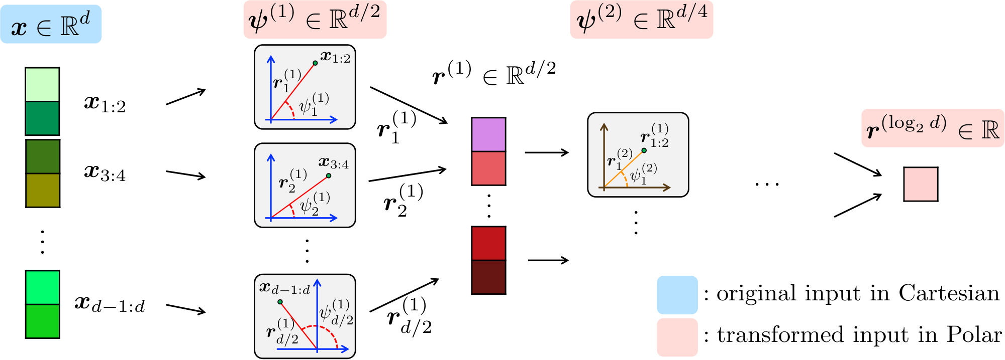
At a high level, our approach begins by grouping pairs of coordinates of a $d$-dimensional vector ${\bm x}$ and transforming each pair into 2D polar coordinates. This produces $d/2$ radius and angle pairs. Next, we gather $d/2$ of radii and apply the polar transform to them. This procedure is recursively repeated $\log_2d$ times and the final output consists of a single final radius and a collection of $1, 2, 4, \dots, d/2$-dimensional angle vectors. A formal definition is provided in Definition 1.

Definition 4: Cartesian to Polar Transformation

For any integer power of two $d$, the polar representation of any vector ${\bm x} \in \mathbb{R}^d$ includes $d-1$ angles and a radius.

Angles are organized into a collection of $\log_2d$ vector of angles $\psi^{(1)}, \psi^{(2)}, \ldots \psi^{(\log_2d)}$ such that $\psi^{(1)} \in [0, 2\pi)^{d/2}$ and $\psi^{(\ell)} \in [0, \pi/2]^{d/2^\ell}$ for any $\ell \ge 2$.

In other words, the angles are computed in $\log_2d$ levels and there are $d/2^\ell$ angles in level $l$.

These angles are defined by the following relation for $\ell \in {2, 3, \ldots \log_2d}$:

$ \begin{align*} \psi^{(1)}{j} &:= \tan^{-1}\left({\bm x}{2j} / {\bm x}{2j-1} \right) ; \text{ for } j \in [d/2], \ \psi^{(\ell)}{j} &:= \tan^{-1}\left(\frac{\left| {\bm x}_{(j-1/2)2^\ell+1:j2^\ell} \right|2 }{ \left| {\bm x}{(j-1)2^\ell+1:(j-1/2)2^\ell} \right|_2 } \right) ; \text{ for } j \in[d/2^\ell]. \end{align*} $

The reverse of this transformation maps the angles and the radius of any point to its Cartesian vector representation using the following equation:

$ \begin{align*} {\bm x}i &= \left| {\bm x} \right|2 \cdot \prod{\ell=1}^{\log_2d} \left(\cos\psi^{(\ell)}{\lfloor \frac{i}{2^\ell} \rfloor} \right)^{\bm{1}{{ (i\text{mod}2^\ell) \le 2^{\ell-1} }}} \cdot \prod{\ell=1}^{\log_2d} \left(\sin\psi^{(\ell)}{\lfloor \frac{i}{2^\ell} \rfloor} \right)^{\bm{1}{{ (i\text{mod}2^\ell) > 2^{\ell-1} }}} \end{align*} $

A visual diagram of the algorithm is shown in Fig. 1 and the pseudocode is provided in Algorithm 1 (see Polar procedure). In what follows, we analyze the distribution of angles generated in each quantization level.

3.2 Distribution of Polar Angles Under Random Preconditioning

One of our primary objectives is to eliminate the need for explicit normalization (e.g., minimum/maximum values) of the KV cache data prior to quantization, thereby reducing quantization overhead. To achieve this, our algorithm applies random preconditioning to the embedding vectors. This preconditioning involves multiplying each embedding vector by a shared random sketch matrix ${\bm S}$ with i.i.d. normal entries. By the Johnson-Lindenstrauss (JL) lemma [36], this preconditioning preserves the norms and inner products[^1] of the embedding vectors with minimal distortion. A key property of this preconditioning, which we will leverage in our later analysis, is that the embedding vectors after preconditioning follow a multivariate normal distribution. This has been formalized in Fact 3.

[^1]: For our implementation, we use random rotation matrices (square matrices $P$ satisfying $P^{\top} P = I$), which preserve the norms and inner products exactly while removing the independence across projected coordinates which we use for our theoretical results.

During the preconditioning stage, the sketch is applied to all embedding vectors in the KV cache, allowing the analysis of PolarQuant to effectively treat the vectors being quantized as samples from a multivariate normal distribution. So for the analysis and design of PolarQuant we can assume without loss of generality that our goal is to quantize a random vector with multivariate Gaussian distribution. A critical insight is that the distribution of angles after random preconditioning becomes predictable and can be analytically derived, which enables the design of optimal quantization schemes.

The polar distribution of a Gaussian vector is derived in the following lemma.

Lemma 5: Distribution of a Gaussian Vector Under Polar Transformation

For an integer power of two $d$, suppose that ${\bm x} \sim \mathcal{N}(0, I_d)$ is a random zero mean isotropic Gaussian random variable in dimension $d$.

Let $\psi_{d}({\bm x}) := \left(\psi^{(1)}, \psi^{(2)}, \ldots \psi^{(\log_2d)} \right)$ denote the set of polar angles obtained by applying the polar transformation defined in on ${\bm x}$.

Denote the radius of ${\bm x}$ by $r = \left| {\bm x} \right|_2$.

The joint probability density function for $\left(r, \psi^{(1)}, \psi^{(2)}, \ldots \psi^{(\log_2d)} \right)$ is the following:

$ f_{R, \Psi_d}(r, \psi_{d}({\bm x})) = f_R(r) \cdot \prod_{\ell=1}^{\log_2d} f_{\Psi^{(\ell)}}\left(\psi^{(\ell)} \right), $

where $f_R(r)$ is the p.d.f. defined in Fact 1, $f_{\Psi^{(1)}}$ is p.d.f. of the uniform distribution over $[0, 2\pi)^{d/2}$:

$ f_{\Psi^{(1)}}: [0, 2\pi)^{d/2} \to (2\pi)^{-d/2}, $

and for every $\ell\in{ 2, 3, \ldots \log_2d }$ the p.d.f. $f_{\Psi^{(\ell)}}$ is the following:

$ \begin{align*} f_{\Psi^{(\ell)}}&: [0, \pi/2]^{d/2^\ell} \to \mathbb{R}+\ f{\Psi^{(\ell)}}(\boldsymbol{\psi}) &= \prod_{i=1}^{d/2^\ell} \frac{\Gamma(2^{\ell-1})}{2^{2^{\ell-1} - 2} \cdot \Gamma(2^{\ell-2})^2} \sin^{(2^{\ell-1}-1)}(2 \psi_i). \end{align*} $

Proof: The proof is by induction on $d$. First for the base of induction we prove the result in dimension $d=2$. So we prove that for a 2-dimensional random Gaussian vector ${\bm y} = (y_1, y_2) \in \mathbb{R}^2$ if $(r, \theta)$ is the polar representation of this vector then following holds:

$ f_{R, \Theta}(r, \theta) = \frac{1}{2\pi} \cdot r \exp\left(-r^2/2 \right), $

To prove this, let $f_Y({\bm y})$ be the probability density function of the vector random variable ${\bm y}$. We know ${\bm y}$ has a normal distribution so we have:

$ \begin{align*} f_{R, \Theta}(r, \theta) &= r \cdot f_Y({\bm y}) = r \cdot \frac{1}{2\pi} e^{-\frac{y_1^2 + y_2^2}{2}} = \frac{1}{2\pi} \cdot r e^{-\frac{r^2}{2}}, \end{align*} $

where the first equality above follows from the change of variable from $(y_1, y_2)$ to $r = \sqrt{y_1^2 + y_2^2}$ and $\theta = \tan^{-1}(y_2 / y_1)$. This proves the base of induction for $d=2$.

Now we prove the inductive step. Suppose that the lemma holds for dimension $d/2$ and we want to prove it for dimension $d$. Denote $\theta := \psi^{(\log_2d)}$, $\boldsymbol{\phi}1 := \left(\psi^{(l)}{1: d/2^{l+1}} \right){\ell=1}^{\log_2d-1}$, $\boldsymbol{\phi}2 := \left(\psi^{(l)}{d/2^{\ell+1}+1: d/2^\ell} \right){\ell=1}^{\log_2d-1}$, $r_1 := \left| {\bm x}{1:d/2} \right|$, and $r_2 := \left| {\bm x}{d/2+1:d} \right|$. Essentially we sliced all the angle vectors $\psi^{(\ell)}$ in half and named the collection of first half vectors $\boldsymbol{\phi}1$ and the collection of second halves $\boldsymbol{\phi}2$. Using the definition of $\psi^{(\ell)}$ 's in , $\boldsymbol{\phi}1$ is exactly the polar transformation of ${\bm x}{1:d/2}$, and $\boldsymbol{\phi}2$ is the polar transformation of ${\bm x}{d/2+1:d}$, so by the definition of $\psi{d}({\bm x})$ in the lemma statement we have $\boldsymbol{\phi}1 = \psi{d/2}({\bm x}{1:d/2})$ and $\boldsymbol{\phi}2 = \psi{d/2}({\bm x}_{d/2+1:d})$. Thus, we can write:

$ \begin{align} &f_{R, \Psi_d}(r, \psi_d({\bm x})) = f_{R, \Theta, \Phi_1, \Phi_2}(r, \theta, \boldsymbol{\phi}1, \boldsymbol{\phi}2) \nonumber \ &= r \cdot f{R_1, R_2, \Phi_1, \Phi_2}(r \cos \theta, r \sin \theta, \boldsymbol{\phi}1, \boldsymbol{\phi}2) \nonumber \ &= r \cdot f{R_1, \Phi_1}(r \cos \theta, \boldsymbol{\phi}1) \cdot f{R_2, \Phi_2}(r \sin \theta, \boldsymbol{\phi}2) \nonumber \ &= r \cdot f{R, \Psi{d/2}}(r_1, \boldsymbol{\phi}1) \cdot f{R, \Psi{d/2}}(r_2, \boldsymbol{\phi}_2), \end{align}\tag{2} $

where the third line above follows from the change of variable from $(r_1, r_2) = (r\cos\theta, r\sin\theta)$ to $r = \sqrt{r_1^2 + r_2^2}$ and $\theta = \tan^{-1}(r_2 / r_1)$. In the fourth line above we used the definition of $\theta = \psi^{(\log_2d)} = \tan^{-1}\left(\frac{\left| {\bm x}_{d/2+1:d} \right|2 }{ \left| {\bm x}{1:d/2} \right|_2 } \right)$ from Definition 1.

Now if we let $f_{\Psi_{d/2}}(\boldsymbol{\phi}1) := \prod{\ell=1}^{\log_2d-1} f_{\Psi^{(\ell)}}\left(\psi^{(\ell)}{1:d/2^{\ell+1}} \right)$ and $f{\Psi_{d/2}}(\boldsymbol{\phi}2) := \prod{\ell=1}^{\log_2d-1} f_{\Psi^{(\ell)}}\left(\psi^{(\ell)}{d/2^{\ell+1}+1:d/2^\ell} \right)$, by the inductive hypothesis we have $f{R, \Psi_{d/2}}(r_1, \boldsymbol{\phi}1) = \frac{2}{2^{d/4} \cdot \Gamma(d/4)} r_1^{d/2-1} \exp\left(-r_1^2/2 \right) \cdot f{\Psi_{d/2}}(\boldsymbol{\phi}1)$ and $f{R, \Psi_{d/2}}(r_2, \boldsymbol{\phi}2) = \frac{2}{2^{d/4} \cdot \Gamma(d/4)} r_2^{d/2-1} \exp\left(-r_2^2 /2 \right) \cdot f{\Psi_{d/2}}(\boldsymbol{\phi}_2)$. Plugging these values into Eq. (2) gives:

$ \begin{align} f_{R, \Psi_{d}}(r, \psi_{d}({\bm x})) &= \frac{4\cdot (r_1 r_2)^{d-1}}{2^{d/2} \Gamma(d/4)^2} \exp\left(-r^2/2 \right) \cdot f_{\Psi_{d/2}}(\boldsymbol{\phi}1) \cdot f{\Psi_{d/2}}(\boldsymbol{\phi}2)\nonumber \ &= \frac{2 r^{d-1} \cdot \sin^{d/2-1} (2\theta)}{2^{3d/2-2} \cdot \Gamma(d/4)^2} e^{ -r^2/2 } \cdot f{\Psi_{d/2}}(\boldsymbol{\phi}1) \cdot f{\Psi_{d/2}}(\boldsymbol{\phi}2) \nonumber \ &= f_R(r) \cdot \frac{\Gamma(d/2)\cdot \sin^{d/2-1} (2\theta)}{2^{d/2-2} \cdot \Gamma(d/4)^2} f{\Psi_{d/2}}(\boldsymbol{\phi}1) \cdot f{\Psi_{d/2}}(\boldsymbol{\phi}2) \nonumber\ &= f_R(r) \cdot f{\Psi_{d}}\left(\psi_{d}({\bm x}) \right), \end{align}\tag{3} $

which completes the inductive proof of this lemma.

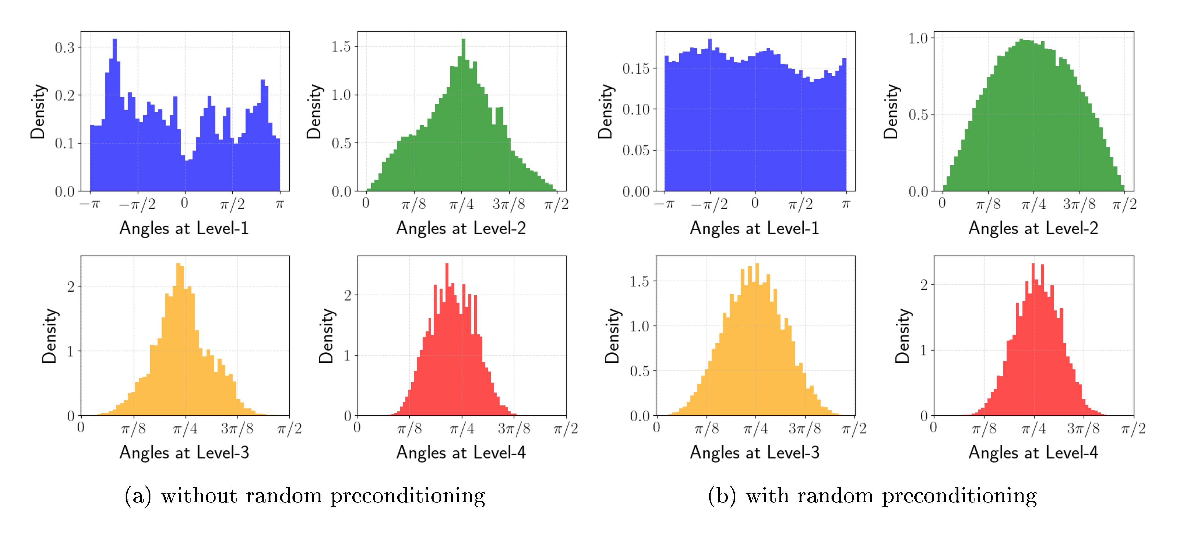
Lemma 2 demonstrates that the angles of Gaussian vectors in polar coordinates have independent distributions, as the probability density function is separable. Moreover, all angles within the same level share identical distributions. Specifically, at level $\ell$ all angles follow the distribution $\psi^{(\ell)}i \sim \prod{i=1}^{d/2^\ell} \frac{\Gamma(2^{\ell-1})}{2^{2^{\ell-1} - 2} \cdot \Gamma(2^{\ell-2})^2} \sin^{2^{\ell-1}-1}\left(2 \psi^{(\ell)}_i \right)$. This density becomes increasingly concentrated around $\pi/4$, particularly at higher levels $\ell$. This property is highly beneficial for reducing quantization error for the angles at higher levels.

**input:** embedding ${\bm X} \in \mathbb{R}^{n \times d}$,
precondition matrix ${\bm S} \in \mathbb{R}^{d \times d}$, bit width $b$
// Cartesian to Polar transform
${\mathbf{R}}_{i}, {\boldsymbol \Psi}^{(1)}_{i}, \dots, {\boldsymbol \Psi}^{(\log_2 d)}_{i} \gets $ $\textsc{Polar}$ $({\bm X}_{i} \cdot {\bm S})$ for $i \in [n]$
// Codebook Construction
Find partition intervals and centroids $( I^{(\ell)}_k, \theta^{(\ell)}_k)_{k \in [2^b]}$ of ${\boldsymbol \Psi}^{(\ell)} \in \mathbb{R}^{n \times (d/2^\ell)}$ that minimize the cost in Eq. (4) for $\ell \in [\log_2 d]$
(See Section 4.1 for details)
// Angles Quantization
${\bm J}_i^{(\ell)} \gets \textsc{Quant}\left({\boldsymbol \Psi}_i^{(\ell)}, (I^{(\ell)}_k, \theta^{(\ell)}_k)_{k \in [2^b]}\right)$ for $i \in [n]$ and $\ell \in [\log_2 d]$
**output:**
${\mathbf{R}} \in \mathbb{R}^{n \times 1}, {\bm J}^{(1)}\in [2^b]^{n \times d/2}, \dots, {\bm J}^{(\log_2 d)} \in [2^b]^{n \times 1}, ( I^{(\ell)}_k, \theta^{(\ell)}_k)_{k \in [2^b]}$

**Procedure** $\textsc{Polar}$ (${\bm y}$)
${\bm r}^{(0)} \gets {\bm y} \in \mathbb{R}^d$
**for** $\ell = 1, \dots, \log_2d$ **do**
  **for** $j = 1, \dots ,{d}/{2^{\ell}}$ **do**
    $\boldsymbol{\psi}^{(\ell)}_j \leftarrow \tan^{-1}\left({\bm r}^{(\ell-1)}_{2j} / {\bm r}^{(\ell-1)}_{2j-1}\right)$
    ${\bm r}^{(\ell)}_j \leftarrow \left\| {\bm r}^{(\ell-1)}_{2j-1:2j} \right\|_2$
  **end for**
**end for**
**output:** ${\bm r}^{(\log_2d)}, {\boldsymbol{\psi}}^{(1)}, \ldots, \boldsymbol{\psi}^{(\log_2d)}$

**Procedure** $\textsc{Quant}$ $\left(\boldsymbol{\psi}, (I_k, \theta_k)_{k \in [2^b]}\right)$
$\boldsymbol{j}_i \gets \mathop{\text{argmin}}_{k \in [2^b]}  \left |\theta_k - \boldsymbol{\psi}_{i}\right|$ for $i \in [d']$ s.t. $\boldsymbol{\psi} \in \mathbb{R}^{d'}$
**output:** $\boldsymbol{j}$

**Procedure** $\textsc{DeQuant}$ $({\bm r}, (\boldsymbol{j}^{(\ell)})_{\ell \in [\log_2 d]}, (\theta_k^{(\ell)})_{k \in [2^b]}, {\bm S})$
**for** $\ell=\log_2d, \dots, 1$ **do**
  **for** $j=1, \dots, d/2^\ell $ **do**
    $i \gets {\boldsymbol j}^{(\ell)}_j$
    ${\bm r}^{(\ell-1)}_{2j-1} \gets {\bm r}^{(\ell)}_{j} \cdot \cos \theta^{(\ell)}_{i}$
    ${\bm r}^{(\ell-1)}_{2j} \gets {\bm r}^{(\ell)}_{j} \cdot \sin \theta^{(\ell)}_{i}$
  **end for**
**end for**
**output:** ${\bm r}^{(0)} \cdot {\bm S}^\top$

3.3 PolarQuant

Algorithm and Main Theorem

PolarQuant starts by first applying random preconditioning, then transforming the vectors into polar coordinates, and finally quantizing each angle. Since Lemma 2 shows that the angles in polar coordinates are independent random variables, each angle can be quantized independently to minimize the total mean squared error. Jointly quantizing multiple angle coordinates offers no additional benefit due to their independence, making our approach both computationally efficient and effective. Therefore, we can focus on one angle at level $l$ and design optimal quantization scheme for it so as to minimize the mean squared error.

Consider an angle $\psi^{(\ell)}i$ at some level $\ell$. According to Lemma 2, its values lie within the range $[0, \pi/2]$ for $\ell\ge2$ and for $\ell=1$ it takes values in the range $[0, 2\pi)$ with a probability density function given by $f\ell(\psi^{(\ell)}_i) := \frac{\Gamma(2^{\ell-1})}{2^{2^{\ell-1} - 2} \cdot \Gamma(2^{\ell-2})^2} \sin^{2^{\ell-1}-1}\left(2 \psi^{(\ell)}_i \right)$. The goal of quantization to $b$-bits is to partition the range $[0, \pi/2]$ (or $[0, 2\pi)$ in case of $\ell=1$) into $2^b$ intervals $I^{(\ell)}_1, I^{(\ell)}2, \cdots I^{(\ell)}{2^b}$ and find corresponding centroids $\theta^{(\ell)}_1, \theta^{(\ell)}2, \ldots \theta^{(\ell)}{2^b}$ such that the following is mean squared error is minimized:

$ \mathop{{\mathbb{E}}}_{\psi^{(\ell)}i \sim f\ell(\psi^{(\ell)}i)}\left[\sum{j \in [2^b]:~ \psi^{(\ell)}_i \in I^{(\ell)}_j} \left| \psi^{(\ell)}_i - \theta^{(\ell)}_j \right|^2 \right].\tag{4} $

This problem is a continuous analog of the k-means clustering problem in dimension 1. Since we have an explicit formula for the p.d.f. of angle $\psi^{(\ell)}i \sim f\ell(\psi^{(\ell)}_i) = \frac{\Gamma(2^{\ell-1})}{2^{2^{\ell-1} - 2} \cdot \Gamma(2^{\ell-2})^2} \sin^{2^{\ell-1}-1}\left(2 \psi^{(\ell)}_i \right)$ the optimal interval partitions and centroids for Eq. (4) can be efficiently computed using numerical methods. For example, one can run k-means clustering on the gathered angle values which can be considered samples from the distribution. This approach ensures minimal quantization error for each angle independently and the overall reconstruction error as well.

We provide a pseudocode of PolarQuant in Algorithm 1. Our main result and error bound are proved in the following.

Theorem 6

For a $d$-dimensional vector ${\bm x} \sim N(0, I_d)$, the polar quantization scheme in uses $O(\log 1/\varepsilon)$ bits per coordinate + the space necessary to store $|{{\bm x}}|_2$, while reconstructing a vector ${\bm x}'$ from such a representation satisfying

$ \begin{align*} \mathop{{\mathbb{E}}}[| {\bm x} - {\bm x}'|_2^2] = \varepsilon \cdot | {\bm x}|_2^2. \end{align*} $

The proof of Theorem 1 can be found in Appendix C. We note that a scheme which uses a deterministic $\varepsilon$-net $\mathcal{N}$ of the unit sphere $\mathbb{S}^{d-1}$, with $|\mathcal{N}| = O(1/\varepsilon)^d$ and rounds the vector $\hat{{\bm x}} = {\bm x}/| {\bm x}|_2$ also uses $O(\log 1/\varepsilon)$ bits per coordinate while achieving the above bounds in the worst case instead of in expectation over the Gaussian distribution. But our construction (i) gives the flexibility to vary the size of the codebook used per each level depending on the resource constraints and as the above theorem shows, can approach the same quality as pinning to an $\varepsilon$-net on average, (ii) does not need to store a $|\mathcal{N}|$-size codebook which is impractical even for modest sizes of $d$ and (iii) has a fast decoding/encoding implementation.

4. KV Cache Quantization with PolarQuant

Section Summary: This section explains how PolarQuant, a compression technique, is used to shrink the memory needed for the KV cache in language models, which stores past data to speed up generating new text tokens. By transforming the data into polar coordinates and quantizing the angles while keeping key points intact, it reduces storage from about 16 bits per data point to roughly 4 bits, saving around four times the memory in models like Llama without major performance drops. The implementation uses recursive transformations over a few levels with custom bit allocations, runs on GPUs via PyTorch and CUDA, and includes a random preprocessing step to improve accuracy, with tests showing strong results on tasks like recalling information from long texts.

In this section, we describe how PolarQuant can be applied to the KV cache problem and our practical implementation. Formally, given a stream of $({\bm q}_1, {\bm k}_1, {\bm v}_1), \ldots, ({\bm q}_n, {\bm k}_n, {\bm v}_n)$, where ${\bm q}_i, {\bm k}i, {\bm v}i \in \mathbb{R}^{d}$ are query, key and value embeddings at $i$-th generation step for all $i \in [n]$. Let ${\bm K}{:i}, {\bm V}{:i} \in \mathbb{R}^{i \times d}$ be matrices defined by stacking ${\bm k}_1, \dots, {\bm k}_i$ and ${\bm v}_1, \dots, {\bm v}_j$ in their rows, respectively. The goal is to compute:

$ \text{softmax}\left(\frac{{\bm K}_{:i} \cdot {\bm q}i}{\sqrt{d}}\right)^T\cdot {\bm V}{:i}.\tag{5} $

For an efficient token generation, the KV cache at $i$-th generation step $({\bm K}{:i}, {\bm V}{:i})$ are stored in the memory. To reduce the memory space, we invoke PolarQuant (Algorithm 1) on these embeddings. Let ${\widehat{ {\bm K} }}{:i}, {\widehat{ {\bm V} }}{:i} \in \mathbb{R}^{i \times d}$ be their dequantizations using DeQuant procedure in Algorithm 1. Then, we estimate Eq. (5) by computing

$ \begin{align} \text{softmax}\left({\frac{{\widehat{ {\bm K} }}_{:i} \cdot {\bm q}i}{\sqrt{d}}}\right) \cdot {\widehat{ {\bm V} }}{:i} . \end{align}\tag{6} $

Note that the naïve cache requires $d \cdot b_{\text{FPN}}$ memory space to store each $d$-dimensional embedding where $b_{\text{FPN}}$ is the number of bits to represent a single floating-point number. If we quantize $\log_2d$ level angles with $b$ bits each and keep centroids in $b_{\text{FPN}}$ bits, the memory space becomes $\left(b_{\text{FPN}} + (d-1)b\right)$. For example, $\mathtt{Llama}$- $\mathtt{3.1}$- $\mathtt{8B}$- $\mathtt{Instruct}$ is represented by $b_{\text{FPN}}=16$ bits and has $d=128$. For $b=3$, we can save the memory space $4.008$ times. In Section 5, the PolarQuant with KV cache marginally degrades the performance of LLMs on various tasks.

4.1 Practical Implementation

The PolarQuant algorithm recursively reduces the dimension of radii by half until the input has dimension 1. We recurse on the polar transformation for a constant $L=4$ levels. Thus, for an embedding of dimension $d$, we obtain $d/16$-dimensional radii and $15d/16$ angle values. We also define different numbers of bits for each quantization level: $b=4$ bits for the first level, and $b=2$ bits for the remaining levels. This is because the range of angle at the first level $[0, 2\pi)$ is $4$ times wider than the others $[0, \pi/2]$. Consequently, the representation of a block of 16 coordinates uses $b_{\text{FPN}} + 32 + 8 + 4 + 2 = b_{\text{FPN}} + 46$ bits that translates to $62 / 16 = 3.875$ bits per coordinate when $b_{\text{FPN}} = 16$ bits.

We implement PolarQuant using the Pytorch [37] framework. Since the smallest data type is represented in 8 bits ($\mathtt{torch.uint8}$), we pack quantized angle indices into 8-bit unit. To accelerate computation on GPU clusters, we implement CUDA kernels for two key operations: (1) the product of query vectors with the dequantized key cache, i.e., ${\widehat{ {\bm K} }}_{:i} \cdot {\bm q}_i$, and (2) the product of attention scores with the dequantized value cache as per Eq. (6). For the preconditioning matrix ${\bm S}$, we generate a random rotational matrix. The matrix ${\bm S}$ is shared across key and value embeddings, as well as all layers and attention heads in the Transformer architecture.

For angle codebook construction (line 3 in ), we use the 1-D k-means++ clustering on either online angles obtained from polar-transformed inputs or offline precomputed angles. Both approaches approximate the solution to by discretizing with samples from angle distributions. While online approach requires additional clustering computation during every prefill stage, this one-time cost is offset by improved performance compared to the offline approach. We present detailed runtime and performance comparisons in Section 5.

5. Experiments

Section Summary: Researchers tested a new method called PolarQuant for compressing key-value caches in AI language models using an NVIDIA RTX A6000 GPU, focusing on how it improves efficiency for handling long texts. In initial tests, preconditioning the cache data made it easier to compress by reshaping its mathematical structure, and in a "needle-in-a-haystack" retrieval task with documents up to 104,000 words long, PolarQuant outperformed competing methods while using only a quarter of the memory. Further evaluations on diverse tasks like question-answering and summarization showed PolarQuant achieving higher accuracy than alternatives, with faster generation speeds than similar quantization techniques, though simpler eviction methods were quicker at the expense of quality.

All experiments are performed with a single NVIDIA RTX A6000 GPU with 48GB VRAM.

5.1 Random Precondition on KV Cache

We first explore the effectiveness of preconditioning. In particular, we choose a single prompt from Qasper dataset in LongBench [38] and extract the corresponding KV cache. To observe how preconditioning improves, we transform the KV cache into 4-level polar coordinates and plot their angle distributions of the key cache. Note that the first level angles are range in $[0, 2\pi)$ and the rest are in $[0, \pi/2]$. The results are illustrated in Fig. 2. As shown in Lemma 2, the distribution of angles get predictably sharper around $\pi/4$ as the level increases. Moreover, we observe that at the first level the preconditioning flattens the angle distribution and removes outliers. This allows us to quantize angles in the KV cache more accurately.

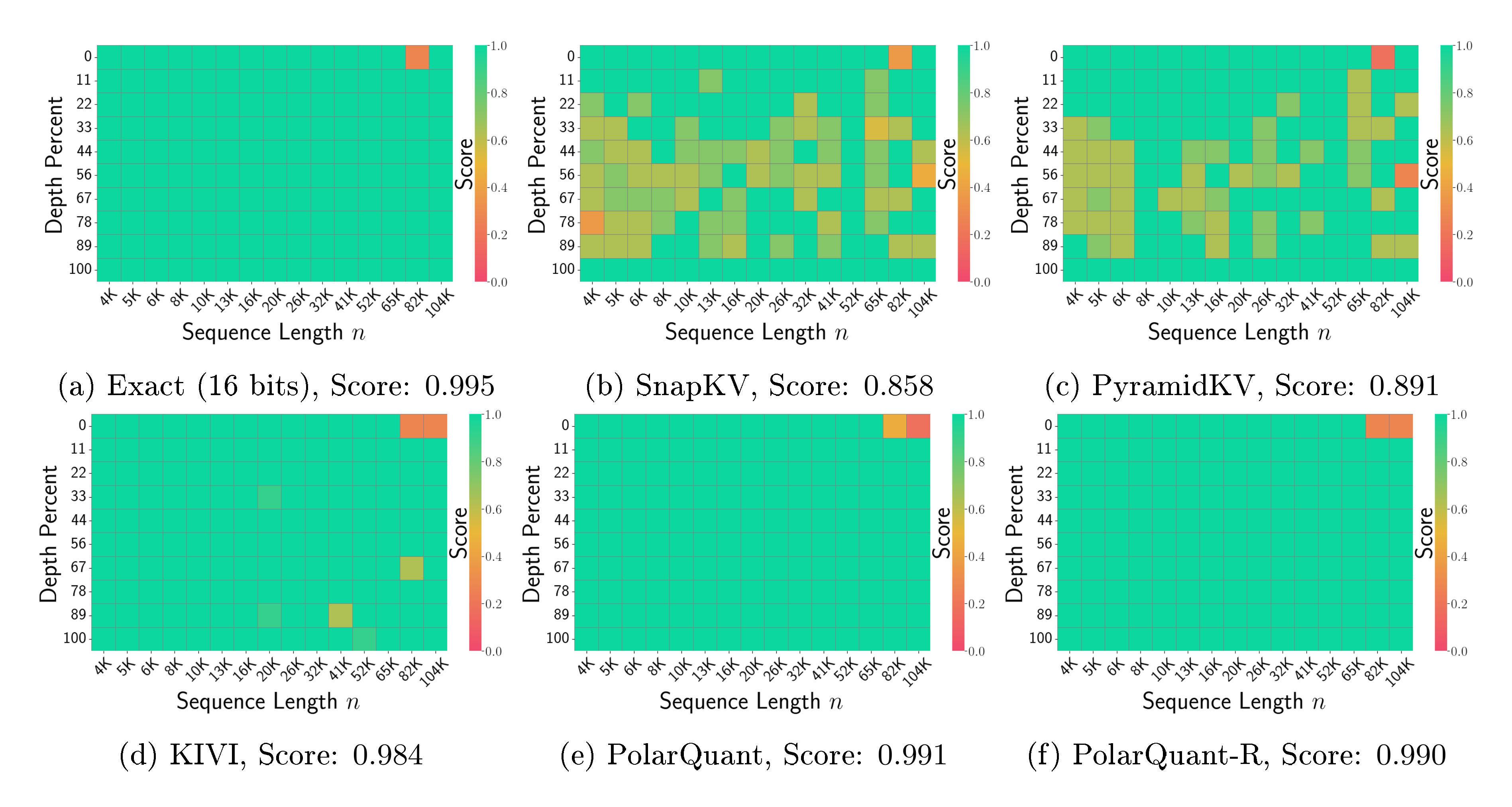
5.2 Needle-In-A-Haystack

Next we evaluate our method for the "Needle-In-A-Haystack" test [39]. It asks the model to retrieve the information in a given sentence where the sentence (the "needle") is placed in an arbitrary location of a long document (the "haystack"). We follow the same setting from Fu et al. [40] and use the $\mathtt{Llama}$- $\mathtt{3.1}$- $\mathtt{8B}$- $\mathtt{Instruct}$ to run the test. We vary the input sequence lengths from 4K to 104K. The evaluation is based on the recall score by comparing the hidden sentence. We compare PolarQuant to SnapKV [21], PyramidKV [41] and KIVI [30], where we use their implementations from [42]. All methods are set to a compression ratio of $0.25$, i.e., required memory is $\times 0.25$ the full KV cache. Specifically, we run our algorithm with and without the preconditioning and refer to them as PolarQuant-R and PolarQuant, respectively. In Fig. 3, we observe that quantization methods (e.g., KIVI, PolarQuant) outperform token-level compression methods (e.g., SnapKV, PyramidKV). PolarQuant shows better scores than KIVI. Additionally, PolarQuant shows a marginally better score than PolarQuant-R.

5.3 End-to-end Generation on LongBench

We run various KV cache compression algorithms for LongBench datasets [38], which encompasses diverse long-text scenarios including single/multi-document question-answering (SQA/MQA), summarization (Sum), few-shot learning (Few), synthetic tasks (Syn), and code completion (Code). Since the number of generated tokens is small compared to the input sequence length across all datasets, we preserve all new streamed query, key, and value pairs from the generation stage in full precision (16 bits) for all methods. We evaluate PolarQuant against the baseline methods using in Section 5.2 as well as StreamingLLM [19] and HeadKV [43] on $\mathtt{Llama}$- $\mathtt{3.1}$- $\mathtt{8B}$- $\mathtt{Instruct}$ .

We investigate two variants of PolarQuant-R: one using online codebook construction and another using offline one discussed in Section 4.1. The online variant performs clustering for each individual input prompt and layer, while the offline one employs a single precomputed codebook that is shared across all input prompts, layers, and attention heads. This offline approach is supported by our findings that the angle distribution, when preconditioned, remains consistent regardless of the input.

As reported in Table 1, our methods achieve superior performance compared to other methods, i.e., the average performance scores are higher by a large margin. This justifies the performance benefits of the quantization of polar coordinates. Moreover, the preconditioned variants (PolarQuant-R) generally demonstrates better performance than the non-preconditioned version. Among them, the online variant performs slightly better than the offline one.

:::

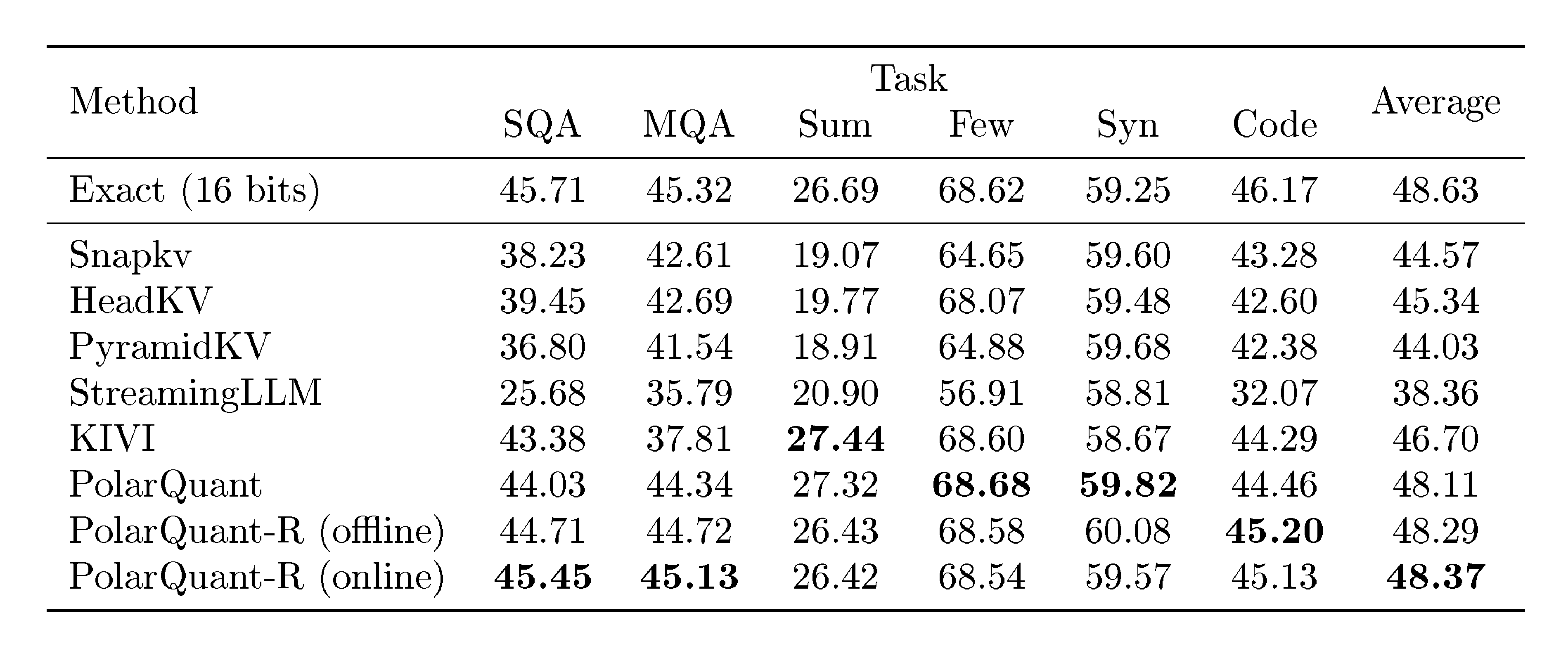
Table 1: LongBench-V1 [38] results of various KV cache compression methods on $\mathtt{Llama}$- $\mathtt{3.1}$- $\mathtt{8B}$- $\mathtt{Instruct}$ . The best values among compression methods are indicated in bold.

:::

:::

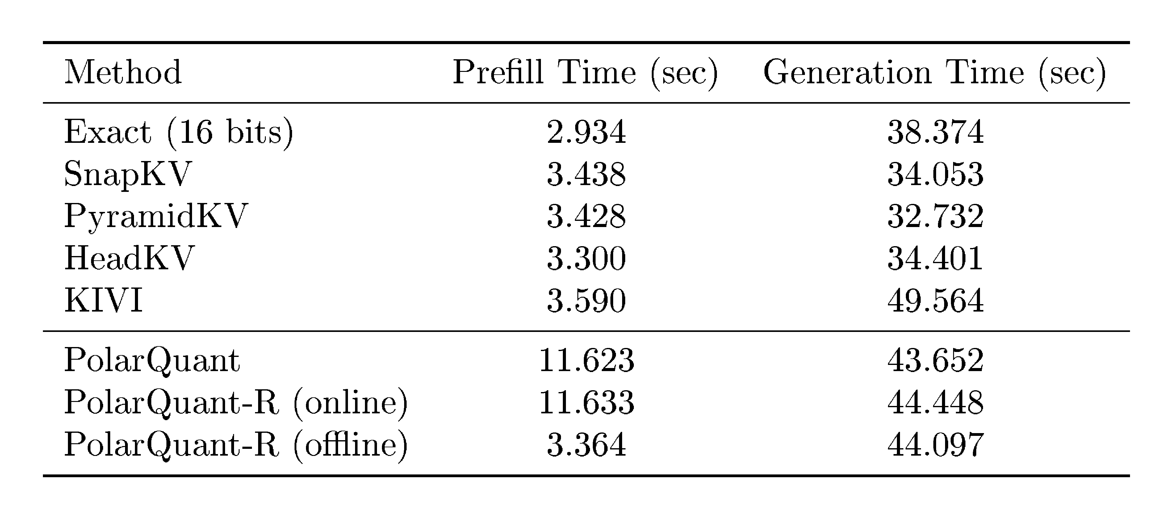
Table 2: Wall-clock runtime comparisons of various KV cache compression methods. The input sequence length is $n=16{, }384$ and the number of generated tokens is $1{, }024$.

:::

5.4 Runtime Analysis

We evaluate wall-clock runtimes of both prefill and token generation stages. Using the Llama model with an input prompt length of $16{, }384$, we measure the time to generate $1{, }024$ tokens for each method. Table 2 summaries the result. Token eviction approaches (SnapKV, PyramidKV, and HeadKV) demonstrate faster generation times compared to exact and quantization methods, though at the cost of lower quality. Among quantization approaches, our PolarQuant algorithms achieve 14% faster generation time than the KIVI while maintaining superior performance. These results demonstrate that PolarQuant offers advantages in both computational efficiency and model performance. To achieve faster prefill times, we recommend using offline codebook construction, as it significantly reduces runtime by eliminating the need for clustering, though this results in a modest performance trade-off. We leave even better codebook construction approaches for future research.

6. Conclusion

Section Summary: PolarQuant is a new technique that simplifies the representation of angles in polar coordinates by quantizing them, which involves connecting to a concept called random preconditioning and providing solid mathematical limits on the errors this causes. When used for compressing the key-value cache in large language models during inference, it cuts down memory use a lot without hurting how well the model performs. This approach could also apply to quantizing model weights and solving broader problems in searching for similar vectors.

We propose PolarQuant, a novel quantization method applied to angles in polar coordinates. We connect it to the random preconditioning which allows us to formalize angle distribution to be quantized. We provide rigorous theoretical bounds on quantization error. When applied to the KV cache compression problem, PolarQuant significantly reduces memory requirements during LLM inference while maintaining model performance. The principles underlying our method extend beyond KV cache compression, offering potential applications in LLM weight quantization and general vector similarity search problems.

Appendix

Section Summary: The appendix contains mathematical proofs supporting the paper's technical claims. It first derives the probability distribution for the length (norm) of a random high-dimensional vector, showing its connection to a chi-squared distribution. Next, it examines the angle formed by two such variables in polar coordinates, proving that this angle averages to 45 degrees with variability shrinking as dimensions increase, and it sketches error estimates for approximating these coordinates through a rounding process.

A. Proof of Fact 1

Proof: The cumulative distribution function (c.d.f) of the random variable $R$ can be computed as follows:

$ \begin{align*} F_R(r) &:= \Pr_{{\bm x}}[\left| {\bm x} \right|2 \le r]\ &= \Pr{{\bm x}}[\left| {\bm x} \right|_2^2 \le r^2] = \frac{1}{\Gamma(d/2)} \gamma(d/2, r^2/2), \end{align*} $

where the last equality is because the squared norm of ${\bm x}$, by definition, is Chi-squared random variable. Differentiating the above c.d.f gives us the p.d.f of $R$:

$ f_R(r) = \frac{2}{2^{d/2} \cdot \Gamma(d/2)} r^{d-1} \exp\left(-r^2/2 \right). \blacksquare $

B. Error Bounds for Polar Quantization

Lemma 7

If $X$ and $Y$ are independent non-negative random variables that are sampled from the generalized gamma distribution with probability density function $f_Z(z) = \frac{2}{2^{d/2} \cdot \Gamma(d/2)}z^{d-1}\exp(-z^2/2)$ so that $X^2, Y^2 \sim \chi^2_d$, then the distribution of $\Theta = \tan^{-1}(Y/X)$ has the pdf

$ \begin{align*} f_{\Theta}(\theta) = \frac{\Gamma(d)}{2^{d-2}\Gamma(d/2)^2}\cdot \sin^{d-1}(2\theta), \quad 0 \le \theta \le \pi / 2. \end{align*} $

We also have that $\mu_{\Theta} = \mathop{{\mathbb{E}}}[\Theta] = \pi/4$ and $\sigma_{\Theta} = \sqrt{\textnormal{Var}(\Theta)} = O(1/\sqrt{d})$.

Proof: Since $X$ and $Y$ are i.i.d., their joint distribution function is the following:

$ \begin{align*} f_{X, Y}(x, y) = f_Z(x) \cdot f_Z(y) = \left(\frac{2}{2^{d/2} \cdot \Gamma(d/2)} \right)^2 (x \cdot y)^{d-1} \exp\left(-(x^2 + y^2)/2 \right). \end{align*} $

Now by changing the coordinates from Cartesian to polar we can represent the above distribution as a joint distribution over variables $r = \sqrt{x^2+y^2}, \theta = \tan^{-1}(y/x)$ with $r \ge 0$ and $\theta \in [0, \pi/2)$ as follows:

$ \begin{align*} f_{R, \Theta}(r, \theta) = r \cdot f_{X, Y}\left(r\cos \theta, r \sin \theta \right) = \frac{r^{2d-1}}{2^{2d - 3} \cdot \Gamma(d/2)^2} \exp\left(-r^2/2 \right) \cdot \sin^{d-1}(2\theta). \end{align*} $

Since the joint probability distribution of $r, \theta$ is a separable function, we can deduce the marginal probability distribution of $\theta$ as follows:

$ \begin{align*} f_{\Theta}(\theta) &= \int_0^\infty f_{R, \Theta}(r, \theta) dr \ &= \frac{ \sin^{d-1}(2\theta) }{2^{2d - 3} \cdot \Gamma(d/2)^2} \cdot \int_0^\infty r^{2d-1} \exp\left(-r^2/2 \right) dr \ &= \frac{ \sqrt{2\pi} \cdot \sin^{d-1}(2\theta) }{2^{2d - 2} \cdot \Gamma(d/2)^2} \cdot \int_{-\infty}^\infty \frac{|r|^{2d-1}}{\sqrt{2\pi}} e^{ -r^2/2 } dr \ &= \frac{ \sqrt{2\pi} \cdot \sin^{d-1}(2\theta) }{2^{2d - 2} \cdot \Gamma(d/2)^2} \cdot \mathop{{\mathbb{E}}}_{r \sim \mathcal{N}(0, 1)} \left[|r|^{2d-1} \right] \ &= \frac{\Gamma(d)}{2^{d - 2} \cdot \Gamma(d/2)^2} \cdot \sin^{d-1}(2\theta), \end{align*} $

where the last equality above follows from Fact 2. For a proof of the mean and variance bound see Lemma 3.

From the symmetry of $f_{\Theta}(\cdot)$ around $\theta = \pi / 4$, it is clear that $\mu_{\Theta} = \pi / 4$. We now bound $\sigma_{\Theta}$.

$ \begin{align*} \text{Var}(\Theta) &= \frac{\Gamma(d)}{2^{d-2}\Gamma(d/2)^2}\int_{0}^{\pi/2}(\theta - \pi / 4)^2 \sin^{d-1}(2\theta), \mathrm{d}\theta\ &= \frac{\Gamma(d)}{2^{d-2}\Gamma(d/2)^2} \int_{-\pi/4}^{\pi/4} \theta^2 \sin^{d-1}(2\theta + \pi / 2), \mathrm{d}\theta\ &= \frac{2\Gamma(d)}{2^{d-2}\Gamma(d/2)^2}\int_{0}^{\pi/4}\theta^2 \cos^{d-1}(2\theta), \mathrm{d}\theta\ &= \frac{\Gamma(d)}{2^{d-3}\Gamma(d/2)^2}\int_{0}^{\pi/4}\theta^2 (1 - 2\sin^2 \theta)^{d-1} \mathrm{d}\theta\ &\le \frac{\Gamma(d)}{2^{d-3}\Gamma(d/2)^2}\int_{0}^{\pi/4}\theta^2 (1 - \frac{8\theta^2}{\pi^2})^{d-1} \mathrm{d}\theta \qquad \text{(since $\sin(x) \ge 2x/\pi$ for $0 \le x \le \pi/2)$}\ &\le \frac{\Gamma(d)}{2^{d-3}\Gamma(d/2)^2}\int_{0}^{\pi/4} \theta^2 \exp\left(-\frac{8(d-1)\theta^2}{\pi^2}\right), \mathrm{d}\theta \qquad \text{(since $1-x \le \exp(-x)$)}\ &\le \frac{\Gamma(d)}{2^{d-3}\Gamma(d/2)^2}\int_{0}^{\infty}\theta^2\exp\left(-\frac{8(d-1)\theta^2}{\pi^2}\right), \mathrm{d}\theta \ . \end{align*} $

Substituting $\beta = 8(d-1)\theta^2/\pi^2$, we have

$ \begin{align*} \text{Var}(\Theta) &\le \frac{\Gamma(d)}{2^{d-3}\Gamma(d/2)^2} \cdot \frac{\pi^3}{32\sqrt{2}(d-1)^{3/2}}\int_{0}^{\infty}\beta^{1/2}\exp(-\beta), \mathrm{d}\beta \le C \frac{\Gamma(d)}{2^{d-3}\Gamma(d/2)^2(d-1)^{3/2}}. \end{align*} $

Assuming $d$ is even and using Stirling approximation, we get

$ \begin{align*} \Gamma(d) = \frac{d!}{d} \approx \frac{\sqrt{2\pi d} \left({d}/{e}\right)^d}{d}, \text{and}, \Gamma(d/2) = \frac{(d/2)!}{(d/2)} \approx \frac{\sqrt{2\pi(d/2)}(d/2e)^{d/2}}{d/2}. \end{align*} $

Therefore,

$ \begin{align*} \text{Var}(\Theta) \le C' \frac{2^d \sqrt{d}}{2^{d-3}(d-1)^{3/2}} \le \frac{C''}{d-1} \end{align*} $

where $C''$ is a universal constant independent of $d$ hence proving the theorem.

C. Proof of Theorem 6

Suppose that $X, Y$ are random variables as in Lemma 7 so that $X^2, Y^2 \sim \chi^2_d$ and define $R = \sqrt{X^2 + Y^2}$ and $\Theta = \tan^{-1}(Y/X)$. Let ${\theta_1, \ldots, \theta_k} \subseteq [0, \pi/2]$ be a codebook and define $\Theta' = \text{round}(\Theta)$ to be the $\theta_i$ nearest to $\Theta$ and $R'$ be an approximation of $R$. We then define

$ \begin{align*} X' = R' \cdot \cos(\text{round}(\Theta))\qquad \text{and}\qquad Y' = R' \cdot \sin(\text{round}(\Theta)) \end{align*} $

to be the reconstructions of $X$ and $Y$ respectively from the rounding scheme, which rounds $\Theta$ using the codebook and the radius $R$ using a recursive approximation. The reconstruction error is defined as

$ \begin{align*} & (X - X')^2 + (Y - Y')^2\ &= (R \cos(\Theta) - R' \cos(\Theta'))^2 + (R \sin(\Theta) - R' \sin(\Theta'))^2\ &= (R \cos(\Theta) - R \cos(\Theta') + R\cos(\Theta') - R'\cos(\Theta'))^2 + (R\sin(\Theta) - R\sin(\Theta') + R\sin(\Theta') -R'\sin(\Theta'))^2. \end{align*} $

Using the fact that $2ab \le (1/\alpha) \cdot a^2 + \alpha \cdot b^2$ for any $\alpha > 0$, we get $(a+b)^2 = a^2 + 2ab + b^2 \le (1 + 1/\alpha)a^2 + (1+\alpha)b^2$ for any $\alpha > 0$. Therefore we have that for any $\alpha > 0$,

$ \begin{align*} (X - X')^2 + (Y - Y')^2 &\le (1+1/\alpha)R^2(\cos(\Theta) - \cos(\Theta'))^2 + (1 + \alpha)(R-R')^2\cos(\Theta')^2\ &\qquad+ (1+1/\alpha)R^2(\sin(\Theta) - \sin(\Theta'))^2 + (1+\alpha)(R-R')^2\sin(\Theta')^2\ &\le (2 + 2/\alpha)R^2(\Theta - \Theta')^2 + (1+\alpha)(R - R')^2, \end{align*} $

where we used that fact that $\sin(\cdot)$ and $\cos(\cdot)$ are 1-Lipschitz and that $\sin^2(\Theta') + \cos^2(\Theta') = 1$.

Now, restricting $\alpha \in (0, 1)$ we get that

$ \begin{align*} \mathop{{\mathbb{E}}}[(X-X')^2 + (Y - Y')^2] \le \frac{4 \mathop{{\mathbb{E}}}[R^2]}{\alpha}\mathop{{\mathbb{E}}}[(\Theta - \Theta')^2] + (1+\alpha)\mathop{{\mathbb{E}}}[(R-R')^2] \end{align*} $

using the independence of $R$ and $\Theta$ and the fact that $\Theta'$ is a deterministic function of $\Theta$ given the codebook ${\theta_1, \ldots, \theta_k}$.

When $d = 1$, we call $\mathop{{\mathbb{E}}}[(X-X')^2 + (Y-Y')^2]$ to be $\text{error}_0$ since it is the expected error in the reconstruction at level 0 and similarly, we call $\mathop{{\mathbb{E}}}[(R-R')^2] = \text{error}_1$ since it is the error in level $1$. We also call $\mathop{{\mathbb{E}}}[(\Theta - \Theta')^2] = \text{quant}_1$ since it is the error of quantizing angles in that level. We therefore have

$ \begin{align*} \text{error}_0 \le \frac{4 \mathop{{\mathbb{E}}}[R^2]}{\alpha} \cdot \text{quant}_1 + (1+\alpha) \cdot \text{error}_1. \end{align*} $

Given a vector $(X_1, \ldots, X_d)$, where each $X_i \sim N(0, 1)$, let $(X'_1, \ldots, X'_d)$ be the reconstructions using $t = \log_2(d)$-level quantization as described in the introduction. Extending the above definitions, we say that $\text{error}_i$ is the total expected error in the reconstructions of level $i$ coordinates in the quantization scheme. Using the above, inequality, we get

$ \begin{align*} \text{error}_0 \le \frac{4d}{\alpha} \cdot \text{quant}_1 + \frac{4d}{\alpha}(1+\alpha) \cdot \text{quant}_2 + \frac{4d}{\alpha}(1+\alpha)^3 \cdot \text{quant}_2 + \cdots + \frac{4d}{\alpha}(1+\alpha)^{t} \cdot \text{quant}t + (1+\alpha)^{t+1} \cdot \text{error}{t+1}, \end{align*} $

where we use the fact that $\mathop{{\mathbb{E}}}[X_1^2 + \cdots + X_d^2] = d$. Since we store the top-level radius exactly, we have $\text{error}_{t+1} = 0$ and therefore,

$ \begin{align*} \frac{\text{error}_0}{d} \le \frac{4}{\alpha}\left(\text{quant}_1 + (1+\alpha) \cdot \text{quant}_2 + \cdots + (1+\alpha)^t \cdot \text{quant}_t\right). \end{align*} $

For each level $i$, given $\varepsilon > 0$, we will now upper bound the size of the codebook for level $i$ so that $\text{quant}_i \le \varepsilon$. It is clear that a codebook ${0, \sqrt{\varepsilon}, 2\sqrt{\varepsilon}, \ldots, 2\pi}$ has a size $\lceil{2\pi/\sqrt{\varepsilon}}\rceil + 1$ and has $\text{quant}_i \le \varepsilon$ irrespective of the distribution of the angles. We would like to use the fact that the distribution of angles gets concentrated with increasing level $i$ to obtain better bounds on the size of the codebook. To that end, we prove the following lemma.

Lemma

Let $X \in [0, \pi/2]$ be an arbitrary random variable with $\text{Var}(X) = \sigma^2$. Given $x$ and a set $S = {x_1, \ldots, x_k}$, define $d(x, S) = \min_{i \in [k]}|x_i - x|$. Define

$ \begin{align*} \text{Var}k(X) := \min{S : |S| = k} E[d(X, S)^2]. \end{align*} $

Given $\varepsilon > 0$, for $k = \Omega(\log(1/\sigma)/\sqrt{\varepsilon})$, we have $\text{Var}_k(X) \le \varepsilon \cdot \text{Var}_1(X) = \varepsilon \cdot \sigma^2$.

The lemma shows that as variance decreases, we can get tighter approximation bounds using the same value of $k$. The proof of this lemma is similar to that of Lemma 2 in Bhattacharya et al. [44].

Proof: Let $\mu = \mathop{{\mathbb{E}}}[X]$. Consider the interval $[\mu - \sigma, \mu + \sigma]$ and consider the points $S_1 = {\mu, \mu \pm \varepsilon \sigma, \mu \pm 2\varepsilon\sigma, \ldots, \mu \pm \sigma}$. Note that $|S_1| = 3 + 2/\varepsilon$. We have

$ \begin{align*} \mathop{{\mathbb{E}}}[d(X, S_1)^2, \mid X \in [\mu - \sigma, \mu + \sigma]] \le \varepsilon^2\sigma^2 \end{align*} $

since every point in the interval $[\mu - \sigma, \mu + \sigma]$ has some point in $S_1$ that is at most $\varepsilon\sigma$ away.

Now define $S_2 = {\mu \pm (1+\varepsilon)^{0}\sigma, \mu \pm (1+ \varepsilon)^1\sigma, \ldots, }$ where the exponent $i$ extends until we have $\mu + (1+\varepsilon)^i\sigma \ge \pi/2$ and $\mu - (1+\varepsilon)^i \sigma \le 0$. Note that we have $|S_2| \le O(\log(1/\sigma)/\varepsilon)$. Suppose $|X-\mu| \in [(1+\varepsilon)^i\sigma, (1+\varepsilon)^{i+1}\sigma]$, then $d(X, S_2) \le \varepsilon(1+\varepsilon)^i\sigma \le \varepsilon|X-\mu|$. Now,

$ \begin{align*} \mathop{{\mathbb{E}}}[d(X, S_1 \cup S_2)^2] \le \mathop{{\mathbb{E}}}[\max(\varepsilon\sigma, \varepsilon|X-\mu|)^2] \le 2\varepsilon^2\sigma^2. \end{align*} $

Thus by putting $\varepsilon \coloneqq \sqrt{\varepsilon/2}$ above, if $k = \Omega(\log (1/\sigma)/\sqrt{\varepsilon})$, then $\text{Var}_k(X) \le \varepsilon\sigma^2$.

Now we consider bounding $\text{quant}i$ by picking an appropriate codebook for level $i$. For all $i > 0$, given a codebook $\mathcal{C} = {\theta_1, \ldots \theta{|\mathcal{C}|}}$, we have $\text{quant}i = \mathop{{\mathbb{E}}}[(\Theta - \text{round}(\Theta, \mathcal{C}))^2]$ where $\Theta$ is $\arctan(Y/X)$ with $Y^2, X^2 \sim \chi^2{2^{i-1}}$. From the lemma above, when $i >1$, we have $\text{Var}(\Theta) \le C/(2^{i-1} - 1)$ and hence, the above lemma shows that there exists a codebook $\mathcal{C}$ of size $|\mathcal{C}| = \Theta(i/\sqrt{\varepsilon})$,

$ \begin{align} \text{quant}_i \le \frac{\varepsilon}{2^{i-1}}. \end{align}\tag{7} $

If we use a codebook of size $O(1/\sqrt{\varepsilon})$ for level 1, we have $\text{quant}_1 \le \varepsilon$ and as described above, for $i \ge 1$, if we use a codebook of size $|\mathcal{C}| = \Theta(i/\sqrt{\varepsilon})$, then $\text{quant}_i \le \varepsilon/(2^{i-1})$ from which we obtain that

$ \begin{align*} \frac{\text{error}_0}{d} \le \frac{4}{\alpha}(2\varepsilon + \frac{1+\alpha}{\varepsilon} (2\varepsilon) + \left(\frac{1+\alpha}{2}\right)^2 (2\varepsilon) + \cdots) \le O(\varepsilon) \end{align*} $

picking $\alpha = 1/2$. Now we compute the number of bits necessary to store the quantized representation of a $d$-dimensional vector. In level $i$, we have $d/2^{i}$ independent samples of $\Theta$ to be quantized and therefore, we need to store $O(\frac{d}{2^{i}} \log(i/\sqrt{\varepsilon}))$ bits for indexing into the codebook for level $i$. Adding over all the levels, we store $O(d\log 1/\sqrt{\varepsilon})$ bits for representing the $d$-dimensional vector and therefore $O(\log 1/\varepsilon)$ bits per coordinate to achieve an average reconstruction error of $\varepsilon$.

References

Section Summary: This references section lists key sources on advanced AI technologies, starting with reports and announcements for prominent language models like GPT-4, Claude, and Gemini, as well as tools for generating images and videos such as DALL-E, Adobe Firefly, Midjourney, Veo, and Sora. It also includes foundational papers on transformer architectures, scaling laws for neural networks, and faster decoding methods that power modern AI systems. The bulk of the citations focus on recent innovations for making large language models more efficient, particularly through techniques like KV cache compression and quantization to handle longer contexts and quicker processing on limited hardware.

[1] Achiam, J., Adler, S., Agarwal, S., Ahmad, L., Akkaya, I., Aleman, F. L., Almeida, D., Altenschmidt, J., Altman, S., Anadkat, S., et al. Gpt-4 technical report. arXiv preprint arXiv:2303.08774, 2023.

[2] Anthropic. Claude, 2024. https://www.anthropic.com/news/claude-3-family.

[3] Google. Gemini 1.5 pro, 2024a. https://arxiv.org/abs/2403.05530.

[4] Ramesh, A., Dhariwal, P., Nichol, A., Chu, C., and Chen, M. Hierarchical text-conditional image generation with clip latents. arXiv preprint arXiv:2204.06125, 2022.

[5] FireFly. Adobe firefly, 2023. https://firefly.adobe.com/.

[6] Midjourney. Midjourney, 2022. https://www.midjourney.com/home.

[7] Google. Veo 2, 2024b. https://deepmind.google/technologies/veo/veo-2/.

[8] OpenAI. Sora: Creating video from text, 2024b. https://openai.com/index/sora/.

[9] Microsoft Copilot. Microsoft copilot, 2023. https://github.com/features/copilot.

[10] OpenAI. Introducing gpt-4o, 2024a. https://openai.com/index/hello-gpt-4o/.

[11] Vaswani, A., Shazeer, N., Parmar, N., Uszkoreit, J., Jones, L., Gomez, A. N., Kaiser, L., and Polosukhin, I. Attention is all you need. NeurIPS, 2017.

[12] Kaplan, J., McCandlish, S., Henighan, T., Brown, T. B., Chess, B., Child, R., Gray, S., Radford, A., Wu, J., and Amodei, D. Scaling laws for neural language models. arXiv preprint arXiv:2001.08361, 2020.

[13] Shazeer, N. Fast transformer decoding: One write-head is all you need. arXiv preprint arXiv:1911.02150, 2019.

[14] Ainslie, J., Lee-Thorp, J., de Jong, M., Zemlyanskiy, Y., Lebron, F., and Sanghai, S. Gqa: Training generalized multi-query transformer models from multi-head checkpoints. In Proceedings of the 2023 Conference on Empirical Methods in Natural Language Processing, pp.\ 4895–4901, 2023.

[15] Dai, D., Deng, C., Zhao, C., Xu, R., Gao, H., Chen, D., Li, J., Zeng, W., Yu, X., Wu, Y., et al. Deepseekmoe: Towards ultimate expert specialization in mixture-of-experts language models. arXiv preprint arXiv:2401.06066, 2024.

[16] Beltagy, I., Peters, M. E., and Cohan, A. Longformer: The long-document transformer. arXiv preprint arXiv:2004.05150, 2020.

[17] Zhang, Z., Sheng, Y., Zhou, T., Chen, T., Zheng, L., Cai, R., Song, Z., Tian, Y., Ré, C., Barrett, C., et al. H2o: Heavy-hitter oracle for efficient generative inference of large language models. Advances in Neural Information Processing Systems, 36, 2024b.

[18] Liu, Z., Desai, A., Liao, F., Wang, W., Xie, V., Xu, Z., Kyrillidis, A., and Shrivastava, A. Scissorhands: Exploiting the persistence of importance hypothesis for llm kv cache compression at test time. Advances in Neural Information Processing Systems, 36, 2024a.

[19] Xiao, G., Tian, Y., Chen, B., Han, S., and Lewis, M. Efficient streaming language models with attention sinks. arXiv preprint arXiv:2309.17453, 2023.

[20] Zandieh, A., Han, I., Mirrokni, V., and Karbasi, A. Subgen: Token generation in sublinear time and memory. arXiv preprint arXiv:2402.06082, 2024b.

[21] Li, Y., Huang, Y., Yang, B., Venkitesh, B., Locatelli, A., Ye, H., Cai, T., Lewis, P., and Chen, D. Snapkv: Llm knows what you are looking for before generation. arXiv preprint arXiv:2404.14469, 2024.

[22] Sheng, Y., Zheng, L., Yuan, B., Li, Z., Ryabinin, M., Chen, B., Liang, P., Ré, C., Stoica, I., and Zhang, C. Flexgen: High-throughput generative inference of large language models with a single gpu. In International Conference on Machine Learning, pp.\ 31094–31116. PMLR, 2023.

[23] Sun, H., Chang, L.-W., Bao, W., Zheng, S., Zheng, N., Liu, X., Dong, H., Chi, Y., and Chen, B. Shadowkv: Kv cache in shadows for high-throughput long-context llm inference. arXiv preprint arXiv:2410.21465, 2024.

[24] Kwon, W., Li, Z., Zhuang, S., Sheng, Y., Zheng, L., Yu, C. H., Gonzalez, J., Zhang, H., and Stoica, I. Efficient memory management for large language model serving with pagedattention. In Proceedings of the 29th Symposium on Operating Systems Principles, pp.\ 611–626, 2023.

[25] Yue, Y., Yuan, Z., Duanmu, H., Zhou, S., Wu, J., and Nie, L. Wkvquant: Quantizing weight and key/value cache for large language models gains more. arXiv preprint arXiv:2402.12065, 2024.

[26] Yang, J. Y., Kim, B., Bae, J., Kwon, B., Park, G., Yang, E., Kwon, S. J., and Lee, D. No token left behind: Reliable kv cache compression via importance-aware mixed precision quantization. arXiv preprint arXiv:2402.18096, 2024.

[27] Dong, S., Cheng, W., Qin, J., and Wang, W. Qaq: Quality adaptive quantization for llm kv cache. arXiv preprint arXiv:2403.04643, 2024.

[28] Kang, H., Zhang, Q., Kundu, S., Jeong, G., Liu, Z., Krishna, T., and Zhao, T. Gear: An efficient kv cache compression recipefor near-lossless generative inference of llm. arXiv preprint arXiv:2403.05527, 2024.

[29] Zhang, T., Yi, J., Xu, Z., and Shrivastava, A. Kv cache is 1 bit per channel: Efficient large language model inference with coupled quantization. arXiv preprint arXiv:2405.03917, 2024a.

[30] Liu, Z., Yuan, J., Jin, H., Zhong, S., Xu, Z., Braverman, V., Chen, B., and Hu, X. Kivi: A tuning-free asymmetric 2bit quantization for kv cache. arXiv preprint arXiv:2402.02750, 2024b.

[31] Hooper, C., Kim, S., Mohammadzadeh, H., Mahoney, M. W., Shao, Y. S., Keutzer, K., and Gholami, A. Kvquant: Towards 10 million context length llm inference with kv cache quantization. arXiv preprint arXiv:2401.18079, 2024.

[32] Zandieh, A., Daliri, M., and Han, I. Qjl: 1-bit quantized jl transform for kv cache quantization with zero overhead. arXiv preprint arXiv:2406.03482, 2024a.

[33] Kim, J., Park, J., Cho, J., and Papailiopoulos, D. Lexico: Extreme kv cache compression via sparse coding over universal dictionaries. arXiv preprint arXiv:2412.08890, 2024.

[34] Shah, J., Bikshandi, G., Zhang, Y., Thakkar, V., Ramani, P., and Dao, T. Flashattention-3: Fast and accurate attention with asynchrony and low-precision. arXiv preprint arXiv:2407.08608, 2024.

[35] Ashkboos, S., Mohtashami, A., Croci, M. L., Li, B., Cameron, P., Jaggi, M., Alistarh, D., Hoefler, T., and Hensman, J. Quarot: Outlier-free 4-bit inference in rotated llms. arXiv preprint arXiv:2404.00456, 2024.

[36] Dasgupta, S. and Gupta, A. An elementary proof of a theorem of johnson and lindenstrauss. Random Structures & Algorithms, 22(1):60–65, 2003.

[37] Paszke, A., Gross, S., Massa, F., Lerer, A., Bradbury, J., Chanan, G., Killeen, T., Lin, Z., Gimelshein, N., Antiga, L., et al. Pytorch: An imperative style, high-performance deep learning library. Advances in neural information processing systems, 32, 2019.

[38] Bai, Y., Lv, X., Zhang, J., Lyu, H., Tang, J., Huang, Z., Du, Z., Liu, X., Zeng, A., Hou, L., Dong, Y., Tang, J., and Li, J. Longbench: A bilingual, multitask benchmark for long context understanding. arXiv preprint arXiv:2308.14508, 2023.

[39] Kamradt, G. Needle in a haystack - pressure testing llms., 2023. https://github.com/gkamradt/LLMTest_NeedleInAHaystack.

[40] Fu, Y., Panda, R., Niu, X., Yue, X., Hajishirzi, H., Kim, Y., and Peng, H. Data engineering for scaling language models to 128k context. arXiv preprint arXiv:2402.10171, 2024b. URL {https://github.com/FranxYao/Long-Context-Data-Engineering}.

[41] Cai, Z., Zhang, Y., Gao, B., Liu, Y., Liu, T., Lu, K., Xiong, W., Dong, Y., Chang, B., Hu, J., et al. Pyramidkv: Dynamic kv cache compression based on pyramidal information funneling. arXiv preprint arXiv:2406.02069, 2024.

[42] Jiang, H., LI, Y., Zhang, C., Wu, Q., Luo, X., Ahn, S., Han, Z., Abdi, A. H., Li, D., Lin, C.-Y., et al. Minference 1.0: Accelerating pre-filling for long-context llms via dynamic sparse attention. In The Thirty-eighth Annual Conference on Neural Information Processing Systems, 2024.

[43] Fu, Y., Cai, Z., Asi, A., Xiong, W., Dong, Y., and Xiao, W. Not all heads matter: A head-level kv cache compression method with integrated retrieval and reasoning. arXiv preprint arXiv:2410.19258, 2024a.

[44] Bhattacharya, A., Freund, Y., and Jaiswal, R. On the k-means/median cost function. Information Processing Letters, 177:106252, 2022. URL https://arxiv.org/pdf/1704.05232.