Mamba-3: Improved Sequence Modeling using State Space Principles

Aakash Lahoti $^{*}$ $^{1}$, Kevin Y. Li$^{*1}$, Berlin Chen$^{*2}$, Caitlin Wang$^{*2}$, Aviv Bick $^{1}$, J. Zico Kolter $^{1}$, Tri Dao $^{\dag}$ $^{23}$, Albert Gu$^{\dag 14}$

$^{*}$ Equal contribution. $^{\dag}$ Equal advising. $^{1}$ Carnegie Mellon University $^{2}$ Princeton University $^{3}$ Together AI $^{4}$ Cartesia AI {alahoti, kyl2, abick, zkolter, agu}@cs.cmu.edu {bc2188, caitlinwang, tridao}@princeton.edu

Abstract

Scaling inference-time compute has emerged as an important driver of LLM performance, making inference efficiency a central focus of model design alongside model quality. While the current Transformer-based models deliver strong model quality, their quadratic compute and linear memory make inference expensive. This has spurred the development of sub-quadratic models with reduced linear compute and constant memory requirements. However, many recent linear models trade off model quality and capability for algorithmic efficiency, failing on tasks such as state tracking. Moreover, their theoretically linear inference remains hardware-inefficient in practice. Guided by an inference-first perspective, we introduce three core methodological improvements inspired by the state space model (SSM) viewpoint of linear models. We combine: (1) a more expressive recurrence derived from SSM discretization, (2) a complex-valued state update rule that enables richer state tracking, and (3) a multi-input, multi-output (MIMO) formulation for better model performance without increasing decode latency. Together with architectural refinements, our Mamba-3 model achieves significant gains across retrieval, state-tracking, and downstream language modeling tasks. At the 1.5B scale, Mamba-3 improves average downstream accuracy by 0.6 percentage points compared to the next best model (Gated DeltaNet), with Mamba-3's MIMO variant further improving accuracy by another 1.2 points for a total 1.8 point gain. Across state-size experiments, Mamba-3 achieves comparable perplexity to Mamba-2 despite using half of its predecessor's state size. Our evaluations demonstrate Mamba-3's ability to advance the performance-efficiency Pareto frontier.

Executive Summary: In the era of large language models, inference efficiency has become as critical as model accuracy, driven by the need for rapid deployment in applications like chatbots, agents, and real-time analysis. Traditional Transformer models, while powerful, suffer from high computational costs and memory demands that grow with sequence length, making them expensive to run at scale. This has spurred interest in alternative architectures, such as state space models, which offer linear compute and constant memory but often lag in performance or practical hardware speed. With AI systems increasingly relying on extended inference for better reasoning, there is an urgent need to advance these efficient models without sacrificing capability.

This document introduces Mamba-3, an upgraded state space model architecture designed to enhance both quality and deployment efficiency over prior versions like Mamba-2. The goal is to evaluate whether targeted improvements can push the balance between model performance and inference speed, enabling more practical AI systems.

The authors developed Mamba-3 by refining the underlying mathematics of state space models through three main changes: a more accurate way to convert continuous dynamics into discrete steps for better expressiveness; complex-valued updates to enable tracking of subtle patterns, such as sequence parities; and a multi-input, multi-output structure to boost computation during inference without slowing it down. They trained models up to 1.5 billion parameters on 100 billion tokens of high-quality text data, comparing against baselines like Transformers, Mamba-2, and Gated DeltaNet across language modeling, retrieval, and synthetic tasks. Evaluations focused on accuracy, perplexity (a measure of prediction quality), state-tracking ability, and real-world hardware performance over periods matching typical training runs, assuming standard GPU setups without custom hardware tweaks.

Key findings include: First, Mamba-3 at 1.5 billion parameters improved average accuracy on downstream language tasks by 1.8 percentage points over the next-best model (Gated DeltaNet), with its multi-output variant adding another 1.2 points for a total gain of about 20% relative to baselines. Second, it halved the required state size compared to Mamba-2 while matching prediction quality, effectively doubling speed for equivalent performance. Third, the complex updates allowed Mamba-3 to solve synthetic state-tracking tasks—like computing parity or modular arithmetic on sequences—nearly perfectly, where Mamba-2 succeeded only at random-guess levels. Fourth, the multi-output design quadrupled computation during inference while keeping wall-clock times similar to Mamba-2, lifting hardware utilization from low-efficiency levels. Finally, optimized software kernels made Mamba-3 up to 20-30% faster in decoding than competitors at common settings.

These results mean Mamba-3 advances the frontier of efficient AI, reducing deployment costs by enabling faster, cheaper inference without quality loss. Unlike Transformers, which balloon in memory for long contexts, Mamba-3's fixed-state design cuts risks in scaling to agentic systems or real-time applications, potentially lowering energy use and hardware needs by 50% or more for similar outputs. It also addresses gaps in prior linear models, like poor pattern retention, which could improve reliability in tasks requiring memory of past data. While expectations were for modest gains, Mamba-3 exceeded them by closing capability holes, signaling that state space models are viable Transformer alternatives in hybrids.

Leaders should prioritize integrating Mamba-3 into hybrid architectures—mixing it with attention layers at a 5:1 ratio—for optimal performance, as pure versions excel in modeling but lag slightly in standalone retrieval (e.g., extracting facts from unstructured text). Trade-offs include slightly longer training times for the multi-output version, but inference benefits outweigh this. Next, conduct pilots on domain-specific data to validate gains, and invest in scaling to larger models (e.g., 7B+ parameters) with refined kernels. Further analysis on diverse datasets, like multilingual or multimodal text, would strengthen deployment decisions.

Limitations include reliance on a single high-quality text corpus, which may not generalize to noisy real-world data, and inherent fixed-state constraints that weaken pure retrieval without hybrid support—though hybrids mitigate this effectively. Confidence is high in core modeling and efficiency gains, backed by rigorous comparisons, but cautious on long-context extrapolation beyond 2,000 tokens without additional norms. Overall, Mamba-3 offers a compelling path to sustainable AI scaling.

1. Introduction

Section Summary: Test-time computing has become crucial for advancing large language models, but traditional Transformer architectures struggle with high memory and processing demands during use. Newer sub-quadratic models like Mamba-2 offer better efficiency by using constant memory and linear computations, yet they still lag in performance, state-tracking abilities, and hardware optimization for real-world deployment. To address these, the authors introduce Mamba-3, incorporating three key improvements—exponential-trapezoidal discretization, complex-valued states, and multi-input multi-output dynamics—that boost language modeling accuracy by up to 2.2 points over competitors, enable solving previously impossible tasks, and achieve similar performance to larger models at half the speed.

Test-time compute has emerged as a key driver of progress in LLMs, with techniques like chain-of-thought reasoning and iterative refinement demonstrating that inference-time scaling can unlock new capabilities ([1, 2]). The rapid rise of parallel, agentic workflows has only intensified the need for efficient inference and deployment of such models ([3, 4]). This paradigm shift makes inference efficiency ([5, 6]) paramount, as the practical impact of AI systems now depends critically on their ability to perform large-scale inference during deployment. Model architecture design plays a fundamental role in determining inference efficiency, as architectural choices directly dictate the computational and memory requirements during generation. While Transformer-based models ([7]) are the current industry standard, they are fundamentally bottlenecked by linearly increasing memory demands through the KV cache and quadratically increasing compute requirements through the self-attention mechanism. These drawbacks have motivated recent lines of work on sub-quadratic models, e.g., state space models (SSMs) and linear attention, which retain constant memory and linear compute while attaining comparable or better performance than their Transformer counterparts. These models have made it into the mainstream, with layers such as Mamba-2 ([8]) and Gated DeltaNet (GDN) ([9, 10]) recently incorporated into large-scale hybrid models that match the performance of pure Transformer alternatives with much higher efficiency ([11, 12, 13, 14]).

Despite the success of linear models, significant progress remains in improving their performance, in particular on advancing the Pareto frontier between model quality and inference efficiency. For example, Mamba-2 was developed to improve training speed and simplicity over Mamba-1 ([15]), by sacrificing some expressivity and thus performing worse for inference-matched models. In addition, they have been shown to lack certain capabilities, such as poor state-tracking abilities, e.g., simply determining parity of bit sequences ([16, 17]). Finally, despite these sub-quadratic models being prized for theoretically efficient inference and thus their widespread adoption, their inference algorithms are not hardware efficient. In particular, because these algorithms were developed from a training perspective, their decoding phase has low arithmetic intensity (the ratio of FLOPs to memory traffic), resulting in large portions of hardware remaining idle.

To develop more performant models from an inference-first paradigm, we introduce three core methodological changes on top of Mamba-2, influenced by an SSM-centric viewpoint of sub-quadratic models.

Exponential-Trapezoidal Discretization.

We provide a simple technique for discretizing time-varying, selective SSMs. Through our framework, we can derive several new discretization methods. One of our instantiations, referred to as "exponential-Euler, " formalizes Mamba-1 and Mamba-2's heuristic discretization that previously lacked theoretical justification. Our new "exponential-trapezoidal" instantiation is a more expressive generalization of "exponential-Euler, " where the recurrence can be expanded to reveal an implicit convolution applied on the SSM input. Combined with explicit $B, C$ bias terms, Mamba-3 can empirically replace the short causal convolution in language model architectures, which was previously hypothesized to be essential for recurrent models.

Complex-valued State Space Model.

By viewing the underlying SSM of Mamba-3 as complex-valued, we enable a more expressive state update than Mamba-2's. This change in update rule, designed to be lightweight for training and inference, overcomes the lack of state-tracking ability common in many current linear models. We show that our complex-valued update rule is equivalent to a data-dependent rotary embedding and can be efficiently computed ([18]), and empirically demonstrate its ability to solve synthetic tasks outside the capabilities of prior linear models.

Multi-Input, Multi-Output (MIMO) SSM.

To improve FLOP efficiency during decoding, we switch from an outer-product–based state update to a matrix-multiplication–based state update. From the view of the signal processing foundations of SSMs, such a transition exactly coincides with the generalization from a single-input single-output (SISO) sequence dynamics to a multiple-input multiple-output (MIMO) one. Here, we find that MIMO is particularly suitable for inference, as the extra expressivity enables more computation during the memory-bound state update during decoding, without increasing the state size and compromising speed.

Put together, these improvements form the core of our Mamba-3 layer. Methodologically, we note that these all arise naturally from an SSM-centric perspective but are not immediate from other popular viewpoints of modern linear layers such as linear attention or test-time regression; we discuss these connections further in Section 5. Empirically, we validate our new model's abilities and capabilities on a suite of synthetic state-tracking and language-modeling tasks.

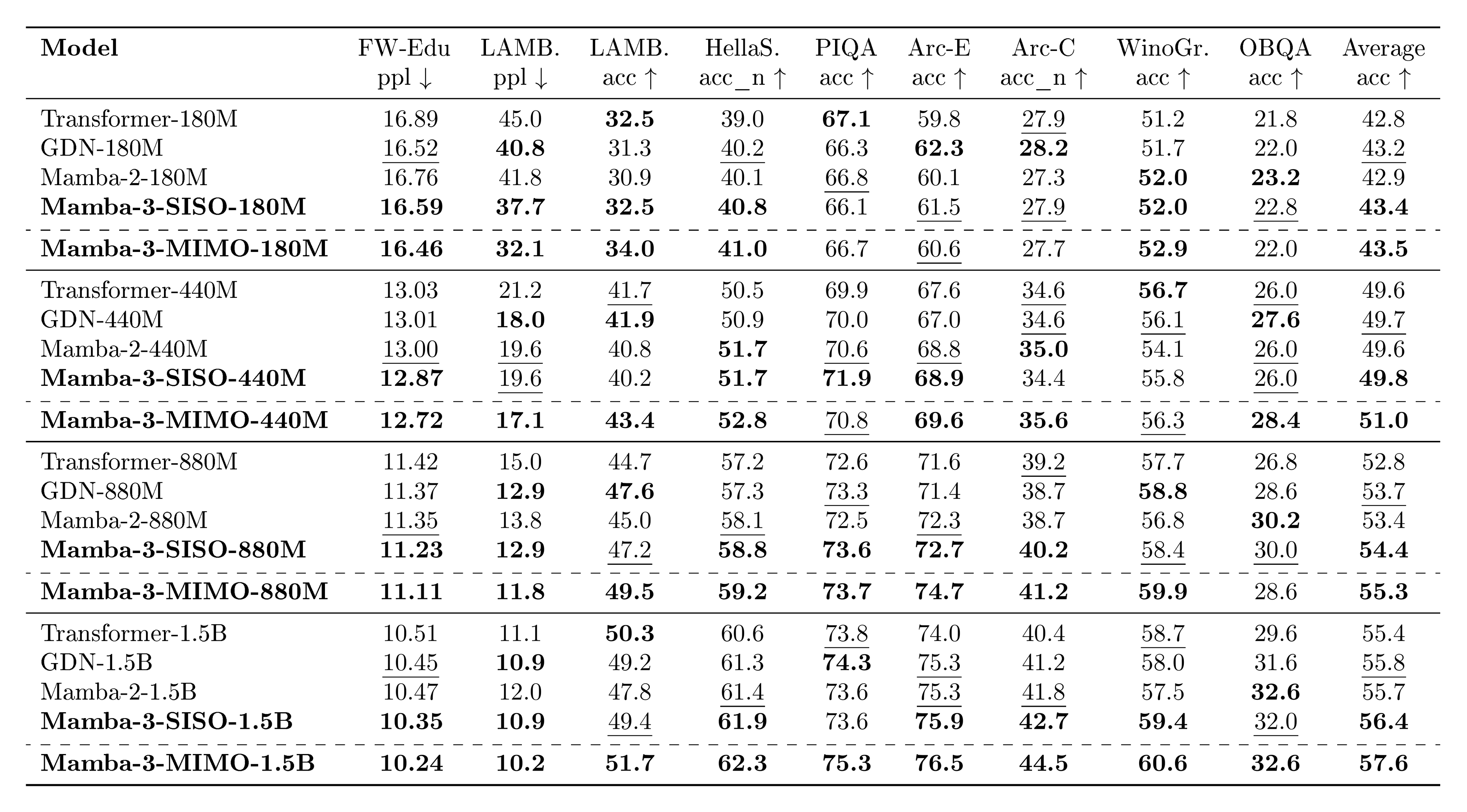
• Better Quality. At 1.5B scale, Mamba-3 (MIMO) improves downstream language modeling accuracy by +2.2 over Transformers, +1.9 points over Mamba-2, and +1.8 over GDN, while Mamba-3 (SISO) improves over the next best model, GDN, by +0.6 points. Furthermore, across state size experiments, Mamba-3 (MIMO) with state size 64 matches the perplexity of Mamba-2 with state size 128, effectively achieving the same language modeling performance with half the latency.
• New Capabilities. Mamba-3's complexification of the SSM state enables it to solve synthetic state-tracking tasks that Mamba-2 cannot. We empirically demonstrate that the efficient RoPE-like calculation is able to near perfectly solve arithmetic tasks, while Mamba-3 without RoPE and Mamba-2 perform no better than random guessing.
• Inference Efficiency. Mamba-3 (MIMO) improves hardware utilization. It increases decoding FLOPs by up to 4 $\times$ relative to Mamba-2 at fixed state size, while maintaining similar wall-clock decode latency, and simultaneously improving perplexity and downstream performance. We release fast training and inference kernels for Mamba-3.^1

Mamba-3 (SISO) improves quality and capability over prior linear models, and Mamba-3 (MIMO) further improves performance over Mamba-3 (SISO) and other strong baselines while matching inference speed with Mamba-2. Both of our Mamba-3 variants advance the performance-latency Pareto frontier through their strong modeling capabilities and hardware-efficient design.

2. Preliminaries

Section Summary: This section introduces basic notation for scalars, tensors, and dimensions used in state space models (SSMs), which are mathematical systems that track hidden states over time based on inputs, evolving from continuous dynamics to discrete steps for computer processing. It details how Mamba-2, a specific SSM design, makes its parameters depend on the input data to efficiently handle sequences on GPUs, with adjustable elements like decay rates that control memory retention and input influence. Finally, it explains the state space duality framework, which reframes these recurrent models as parallel matrix operations with structured masks, linking SSMs to attention mechanisms and showing how Mamba-3 extends Mamba-2 for greater expressiveness.

2.1 Notation

Scalars are denoted by plain-text letters (e.g., $x, y$). Tensors, including vectors and matrices, are denoted by bold letters (e.g., ${\bm{h}}, {\bm{C}}$). The shape of the tensor can be inferred from the context. We denote the input sequence length as $T$, the model dimension as $D$, and the SSM state size as $N$. For time indices, we use subscripts (e.g., $x_t$ for the input at time $t$). The Hadamard product between two tensors is denoted by $\odot$. For a vector ${\bm{v}} \in \mathbb{R}^d$, we denote $\mathrm{Diag}({\bm{v}}) \in \mathbb{R}^{d \times d}$ as the diagonal matrix with the vector ${\bm{v}}$ as the diagonal, and for products of scalars across time steps, we use the notation $\alpha_{t \cdots s} = \alpha^\times_{t:s} = \prod_{i=s}^{t} \alpha_i$.

2.2 SSM Preliminaries

State Space Models (SSMs) describe continuous-time linear dynamics via

$ \begin{align*} \dot{{\bm{h}}}(t) &= {\bm{A}}(t), {\bm{h}}(t) + {\bm{B}}(t), x(t), & y(t) &= {\bm{C}}(t)^\top {\bm{h}}(t), \end{align*} $

where ${\bm{h}}(t)!\in!\mathbb{R}^N$ is the hidden state, $x(t)!\in!\mathbb{R}$ the input, and ${\bm{A}}(t)!\in!\mathbb{R}^{N\times N}$, ${\bm{B}}(t), {\bm{C}}(t)!\in!\mathbb{R}^N$. We will occasionally refer to ${\bm{A}}(t)$ as the state-transition and ${\bm{B}}(t)x(t)$ as the state-input; this also extends to their discretized counterparts. For discrete sequences with step size $\Delta_t$, Mamba-1 and Mamba-2 discretized the system to the following recurrence

$ \begin{align*} {\bm{h}}_t &= e^{\Delta_t {\bm{A}}t}, {\bm{h}}{t-1} + \Delta_t, {\bm{B}}_t, x_t, & y_t &= {\bm{C}}_t^\top {\bm{h}}_t . \end{align*} $

Mamba-2's Parameterization.

The core of the Mamba-2 layer ([8]) is a data-dependent and hardware-efficient SSM. Both the state-transition and state-input are made data-dependent through the projection of $\Delta_t \in \mathbb{R}_{>0}$ and ${\bm{B}}, {\bm{C}}\in\mathbb{R}^N$ from the current token. By parameterizing the state-transition ${\bm{A}}t$ as a scalar times identity (${\bm{A}}t = A_t \bm{I}{N\times N}$, where $A_t \in \mathbb{R}{<0}$), the SSM recurrence can be efficiently computed with the matrix multiplication tensor cores of GPUs. Defining $\alpha_t \coloneqq e^{\Delta_t A_t}\in(0, 1)$ and $\gamma_t \coloneqq \Delta_t$, the update becomes

$ {\bm{h}}t = \alpha_t, {\bm{h}}{t-1} + \gamma_t, {\bm{B}}_t, x_t, \qquad y_t = {\bm{C}}_t^\top {\bm{h}}_t .\tag{1} $

The data-dependent state-transition $\alpha_t$ controls the memory horizon of each SSM within the layer. $\Delta_t$ in particular modulates both the state-transition and state-input: a larger $\Delta_t$ forgets faster and up-weights the current token more strongly, while a smaller $\Delta_t$ retains the hidden state with minimal contributions from the current token.

Remark

In Mamba-2, $A_t$ is data-independent, since the overall discrete transition $\alpha_t \coloneqq e^{\Delta_t A_t}$ is data-dependent through $\Delta_t$.

In Mamba-3, we empirically found that data-dependent $A_t$ has similar performance to data-independent $A_t$, and chose the former as a default for consistency so that all SSM parameters are data-dependent.

2.3 Structured Masked Representation and State Space Duality

Mamba-2 showed that a large class of SSMs admit a matrix form that vectorizes the time-step recurrence. Through the state space duality (SSD) framework, recurrent SSMs can be represented within a parallel form that incorporates an element-wise mask to model the state-transition decay.

SSD provides a general framework for a duality between linear recurrence and parallelizable (matrix-multiplication-based) computational forms

$ \begin{align} {\bm{Y}}

({\bm{L}} \odot {\bm{C}} {{\bm{B}}}^{\top}){\bm{X}} \end{align}\tag{2} $

where ${\bm{L}} \in \mathbb{R}^{T \times T}$ is a structured mask, ${\bm{B}}, {\bm{C}} \in \mathbb{R}^{T \times N}$, ${\bm{X}} \in \mathbb{R}^{T \times D}$ are the inputs to the SSM and ${\bm{Y}} \in \mathbb{R}^{T \times D}$ is its output. Different structures on ${\bm{L}}$ give rise to various instantiations of SSD.

Equation (2) also draws a general connection between recurrence and attention, by setting ${\bm{Q}}\coloneqq {\bm{C}}$, ${\bm{K}}\coloneqq {\bm{B}}$, ${\bm{V}}\coloneqq {\bm{X}}$ and viewing ${\bm{L}}$ as a data-dependent mask. In fact, the simplest case of SSD is (causal) linear attention ([19]), where ${\bm{L}}$ is the causal triangular mask.

Mamba-2 is a generalization where

$ \begin{align} {\bm{L}}

\begin{bmatrix} 1 \ \alpha_1 & 1 \ \vdots & & \ddots \ \alpha_{T...1} & \cdots & \alpha_T & 1 \end{bmatrix} \cdot \operatorname*{Diag}(\gamma) \end{align}\tag{3} $

composed of terms $\alpha_t, \gamma_t$ from equation (1). [^2]

[^2]: In the original Mamba-2 paper, $\gamma$ does not appear because it is viewed as folded into the ${\bm{B}}$ term. In this paper, ${\bm{B}}_t$ represents the continuous parameter, whereas in Mamba-2, ${\bm{B}}_t$ represents the discretized parameter which is equivalent to $\gamma_t {\bm{B}}_t$.

In Section 3.1.3, we show that Mamba-3 is a generalization of Mamba-2 with a more expressive ${\bm{L}}$, and hence also an instance of SSD.

3. Methodology

Section Summary: The methodology section introduces Mamba-3, an advanced state space model that improves on existing designs through three key innovations: a new "exponential-trapezoidal" discretization technique for capturing more dynamic patterns in data, complex-valued states to better track information over time, and multi-input multi-output systems to enhance overall modeling strength and computational efficiency. These changes tackle limitations in current models that process sequences without the heavy resource demands of traditional transformers. Specifically, the first innovation refines how continuous mathematical systems are converted into discrete steps for handling real-world data like text or signals, building on and justifying methods from earlier versions while offering a more precise and flexible approach.

We introduce Mamba-3, a state space model with three new innovations: "exponential-trapezoidal" discretization for more expressive dynamics (Section 3.1), complex-valued state spaces for state tracking (Section 3.2), and multi-input multi-output (MIMO) to improve modeling power and inference-time hardware utilization (Section 3.3). These advances address the quality, capability, and efficiency limitations of current sub-quadratic architectures. We combine these together into an updated Mamba architecture block in Section 3.4.

3.1 Exponential-Trapezoidal Discretization

Structured SSMs are naturally defined as continuous-time dynamical systems that map input functions, $x(t) \in \mathbb{R}$, to output functions, $y(t) \in \mathbb{R}$, for time $t > 0$. The underlying continuous state space system is defined by a first-order ordinary differential equation (ODE) for the state $\dot{{\bm{h}}}(t)$ and an algebraic equation for the output $y(t)$. In sequence modeling, however, the data is only observed at discrete time steps, which then requires applying a discretization step to the SSM to transform its continuous-time dynamics into a discrete recurrence.

Discretization methods are well-studied in classical control theory with several canonical formulas used in earlier SSM works in deep learning ([20, 21, 22]). These mechanisms were traditionally stated and applied to linear-time invariant (LTI) systems, and their derivations do not directly apply to linear-time varying (LTV) systems. Additionally, while Mamba-1 adapted the zero-order hold (ZOH) method to LTV systems without proof, the complexity associated with selective SSMs prompted the use of an additional heuristic approximation that lacked theoretical justification and did not correspond to any established discretization technique. In the following subsection, we formalize the previous heuristics used in current LTV SSMs through our discretization framework and utilize it to propose a more expressive discretization scheme.

3.1.1 Overview of Exponential-Adjusted Discretization

We introduce a simple derivation that leads to a class of new discretization methods for LTV state space models. The method can be instantiated in various ways; we show that one instantiation results in the heuristic used in Mamba-1/2, thereby theoretically justifying it (exponential-Euler). We also introduce a more powerful discretization (exponential-trapezoidal) used in Mamba-3.

The high-level intuition of our derivation originates from the closed form solution $x(t) = e^{tA}x(0)$ of a simple linear ODE $x'(t) = Ax(t)$, which discretizes to $x_{t+1} = e^{\Delta A}x_t$. In this example, the exponential dominates the dynamics of the underlying first-order ODE, resulting in imprecise approximations when using low-order methods without significantly constraining $\Delta$. Thus, we analyze the dynamics of the exponential-adjusted system $e^{-At}x(t)$. The adjusted system yields a discrete recurrent form where the state-transition and the state-input integrals are approximated separately—the state-transition integral is approximated by a right-hand approximation, i.e. $A(s) \coloneqq A(\tau_t)$ for all $s \in [\tau_{t-1}, \tau_t]$, yielding,

$ \begin{align*} {\bm{h}}(\tau_t) &= \underbrace{\exp\left(\int_{\tau_{t-1}}^{\tau_t}A(s)ds\right){\bm{h}}(\tau_{t-1})}\text{via right-hand approximation} + \underbrace{\int{\tau_{t-1}}^{\tau_t} \exp\left(\int_{\tau}^{\tau_t}A(s)ds\right){\bm{B}}(\tau)x(\tau) d\tau}\text{via different discretization schemes}, \ {\bm{h}}t &\approx \exp\left(\Delta_t A_t\right){\bm{h}}{t-1} + \int{\tau_{t-1}}^{\tau_t} \exp\left((\tau_t -\tau)A_t\right){\bm{B}}(\tau)x(\tau) d\tau, \end{align*} $

which serves as the foundation for further discretization techniques for the state-input integral. The full derivation is detailed in Proposition 5.

ZOH.

The classical zero-order hold discretization method can be derived from the foundation above with a specific approximation of the right-hand side integral. By treating $A_t, {\bm{B}}(\tau), x(\tau)$ as constants over the interval $[\tau_{t-1}, \tau_t]$ where the values are fixed to the right endpoint $\tau_t$, the integral results in $A_t^{-1}, \left(\exp(\Delta_tA_t) - I\right){\bm{B}}_tx_t$.

We note that this formally proves that the classical ZOH formula for LTI systems applies to LTV by naively replacing the parameters $A, B, \Delta$ with their time-varying ones.

Exponential-Euler (Mamba-1/-2).

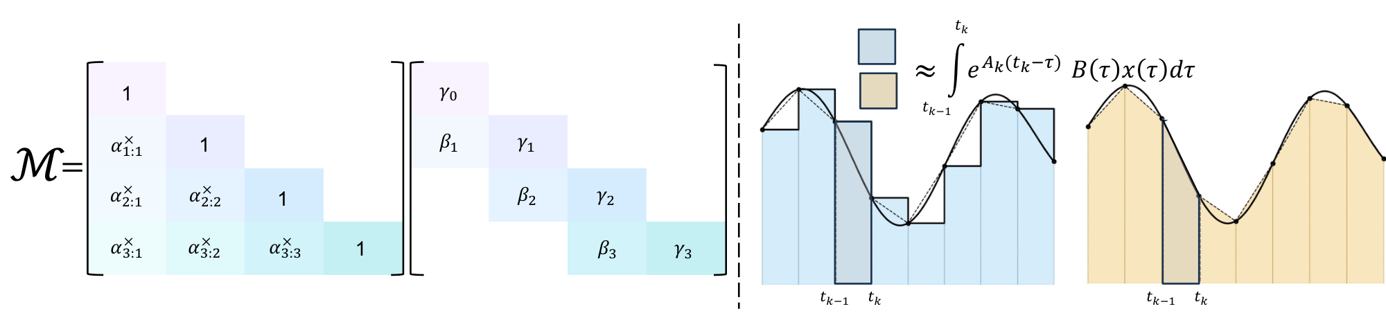
While Mamba-1 stated to use the time-varying ZOH formula above, Mamba-1 and Mamba-2 actually used an additional approximation in the released implementation. This discretization can be recovered by approximating the state-input integral with Euler's rule ([23]) and holding the (right) endpoint constant throughout the interval (Figure 1)

$ \begin{align} {\bm{h}}t ;&\approx; e^{\Delta_t A_t}, {\bm{h}}{t-1} ;+; (\tau_t - \tau_{t-1}) e^{(\tau_t-\tau_t) A_t}, {\bm{B}}t, x_t \nonumber \ &=; e^{\Delta_t A_t}, {\bm{h}}{t-1} ;+; \Delta_t, {\bm{B}}_t, x_t. \end{align}\tag{4} $

We call equation (4) the exponential-Euler discretization method, stemming from the exponential integration followed by Euler approximation. This derivation justifies the formulas used in Mamba-1/-2's implementation.

Exponential-Trapezoidal (Mamba-3).

However, Euler's rule provides only a first-order approximation of the state-input integral and its local truncation error scales as $O(\Delta_t^2)$. In contrast, we introduce a generalized trapezoidal rule, which provides a second-order accurate approximation of the integral, offering improved accuracy over Euler's rule. Specifically, it approximates the integral with a data-dependent, convex combination of both interval endpoints. This generalization extends the classical trapezoidal rule ([23]), which simply averages the interval endpoints (Figure 1).

Proposition 1: Exponential-Trapezoidal Discretization

Approximating the state-input integral in equation (10ab) by the general trapezoidal rule yields the recurrence,

$ \begin{align} {\bm{h}}t ;&=; e^{\Delta_t A_t} {\bm{h}}{t-1} ;+; (1-\lambda_t)\Delta_t e^{\Delta_t A_t} {\bm{B}}{t-1} x{t-1} ;+; \lambda_t \Delta_t {\bm{B}}t x_t, \ &\eqqcolon; \alpha_t {\bm{h}}{t-1} ;+; \beta_t {\bm{B}}{t-1} x{t-1} ;+; \gamma_t {\bm{B}}_t x_t, \end{align}\tag{5} $

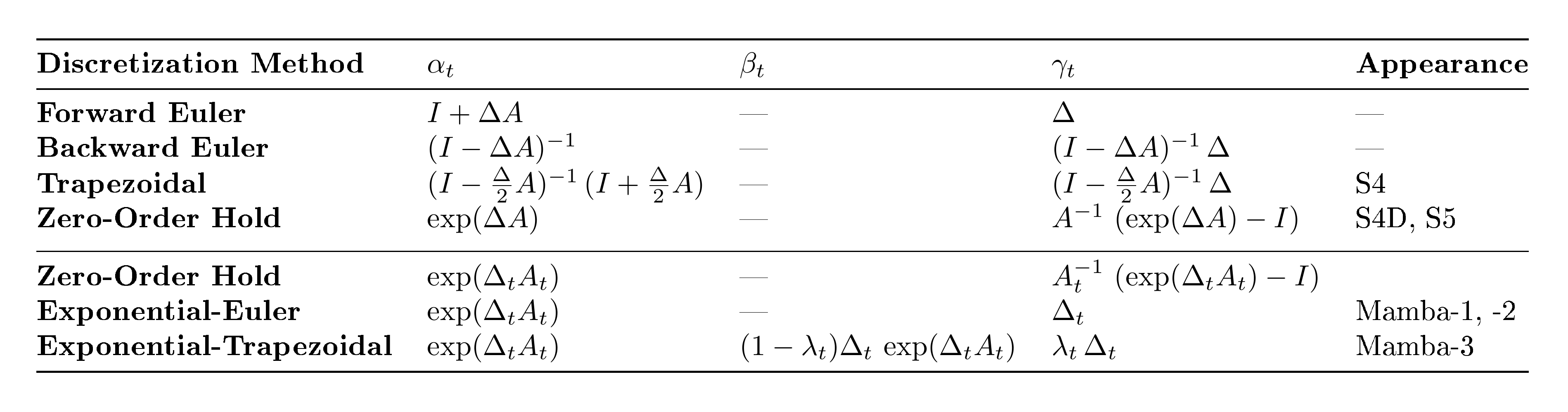
where $\lambda_t \in [0, 1]$ is a data-dependent scalar, $\alpha_t \coloneqq e^{\Delta_t A_t}$, $\beta_t \coloneqq (1-\lambda_t)\Delta_t e^{\Delta_t A_t}$, $\gamma_t \coloneqq \lambda_t \Delta_t$.

Remark: Expressivity

The exponential-trapezoidal rule is a generalization of (a) the classical trapezoid rule, which is recovered when $\lambda_t = \tfrac{1}{2}$, and (b) Mamba-2's Euler's rule, which is recovered when $\lambda_t = 1$.

Remark: Error Rate

This is a second-order discretization of the state-input integral and its error scales as $O(\Delta_t^3)$ under standard stability assumptions, provided that the trapezoidal parameter satisfies $\lambda_t = \tfrac{1}{2} + O(\Delta_t)$.

However, our ablations indicate that not enforcing this constraint is better for empirical performance. See Appendix A.2 and Appendix A.3 for details.

Our new discretization framework and the two instantiations, exponential-Euler and exponential-trapezoidal, are, to the best of our knowledge, novel for structured SSMs used in deep learning. Table 1 compares and summarizes canonical and commonly used discretization schemes for state space models.

3.1.2 Exponential-Trapezoidal Recurrence as an Implicit Convolution

Our generalized exponential-trapezoidal discretization is equivalent to applying a data-dependent convolution of size two on the state-input to the SSM. In particular, a normal SSM in recurrent form materializes the state-input ${\bm{v}}_t = {\bm{B}}_tx_t$, then computes a linear recurrence ${\bm{h}}t = \alpha_t {\bm{h}}{t-1} + \gamma_t {\bm{v}}_t$. In equation (5) we instead first apply a width-2 convolution on ${\bm{v}}_t$ (weighted by $\beta, \gamma$) before passing it into the linear recurrence.

Remark: Convolution Differences

There is a distinct difference between the "convolution" induced by exponential-trapezoidal discretization and the standard short convolutions used by sequence models such as Mamba and GDN.

Standard short convolutions are independent operations applied on $x_t$ (and often ${\bm{B}}_t, {\bm{C}}_t$) outside the core recurrence, while our new discretization can be interpreted as a convolution on the state-input ${\bm{B}}_t x_t$ within the core recurrence.

3.1.3 Parallel Representation of Exponential-Trapezoidal Recurrence

Our new recurrence can be instantiated as a case of SSD and has a corresponding parallel form to equation (2). Expanding the state recurrence from ${\bm{h}}_0 = \gamma_0 {\bm{B}}_0 x_0$ results in ${\bm{h}}T = \alpha{T\cdots 2}(\gamma_0\alpha_1 + \beta_1){\bm{B}}_0x_0 + \cdots + \gamma_T {\bm{B}}_T x_T$, where the SSM output is ${\bm{y}}T = \alpha{T\cdots 2}(\gamma_0\alpha_1 + \beta_1) {\bm{C}}_T^\top {\bm{B}}_0 x_0 + \cdots + \gamma_T {\bm{C}}_T^\top {\bm{B}}_T x_T$. Unrolling these rows shows that the mask induced by the trapezoidal update is no longer a fixed averaging of endpoints (as in the classical trapezoid rule), but a data-dependent convex combination of the two interval endpoints.

Under the SSD framework Equation (2) with parallel form ${\bm{Y}} = ({\bm{L}} \odot {\bm{C}} {{\bm{B}}}^{\top}){\bm{X}}$, Mamba-3 corresponds to a mask ${\bm{L}}$ whose structure is a 1-semiseparable matrix composed with a 2-band matrix:[^3]

[^3]: Incidentally, this is a special case of a 2-semiseparable matrix.

$ \begin{align} {\bm{L}} = \begin{bmatrix} \gamma_0 & & & \ (\gamma_0\alpha_1 + \beta_1) & \gamma_1 & & \ \alpha_2(\gamma_0\alpha_1 + \beta_1) & (\gamma_1\alpha_2+\beta_2) & \gamma_2 & \ \vdots & & & \ddots \ \alpha_{T\cdots 2}(\gamma_0\alpha_1 + \beta_1) & & & \cdots & \gamma_T \end{bmatrix} = \begin{bmatrix} 1 & & & \ \alpha_1 & 1 & & \ \alpha_2\alpha_1 & \alpha_2 & 1 & \ \vdots & & & \ddots \ \alpha_{T\cdots 1} & & & \cdots & 1 \end{bmatrix} \begin{bmatrix} \gamma_0 & & & \ \beta_1 & \gamma_1 & & \ 0 & \beta_2 & \gamma_2 & \ \vdots & & & \ddots \ 0 & & & \cdots & \gamma_T \end{bmatrix}. \end{align}\tag{6} $

This parallel formulation enables the hardware-efficient matmul-focused calculation of the SSM output for training.

We note that the convolutional connection of Mamba-3 can also be seen through this parallel dual form, where multiplication by the 2-band matrix in equation (6) represents convolution with weights $\beta, \gamma$. In Appendix A.1, we use the SSD tensor contraction machinery to prove that the parallel form is equivalent to a vanilla SSM with a state-input convolution.

Remark

The structured mask of Mamba-3 can be viewed as generalizing Mamba-2, which instead of the 2-band matrix has a diagonal matrix with $\gamma_t$ only Equation (3).

3.2 Complex-Valued SSMs

Modern SSMs are designed with efficiency as the central goal, motivated by the need to scale to larger models and longer sequences. For instance, successive architectures have progressively simplified the state-transition matrix: S4 ([20]) used complex-valued Normal Plus Low Rank (NPLR) matrices, Mamba ([15]) reduced this to a diagonal of reals, and Mamba-2 ([8]) further simplified it to a single scaled identity matrix. Although these simplifications largely maintain language modeling performance, recent works ([24, 17, 16]) have shown that the restriction to real, non-negative eigenvalue transitions degrades the capabilities of the model on simple state-tracking tasks—here referring primarily to the solvable-group regime ($\text{TC}^0$) such as parity—which can be solved by a one-layer LSTM. This limitation, formalized in Theorem 1 of ([25]), arises from restricting the eigenvalues of the transition matrix to real numbers, which cannot represent "rotational" hidden state dynamics. For instance, consider the parity function on binary inputs ${0, 1}$, defined as $\sum_t x_t \bmod 2$. This task can be performed using update: ${\bm{h}}t = {\bm{R}}(\pi x_t) {\bm{h}}{t-1}$, where ${\bm{R}}(\cdot)$ is a 2-D rotation matrix. Such rotational dynamics cannot be expressed with real eigenvalues.

3.2.1 Complex SSM with Exponential-Euler Discretization

To recover this capability, we begin with complex SSMs Equation (7), which are capable of representing state-tracking dynamics. We show that, under discretization (Proposition 5), complex SSMs can be formulated as real SSMs with a block-diagonal transition matrix composed of $2 \times 2$ rotation matrices (Proposition 2). We then show that this is equivalent to applying data-dependent rotary embeddings on both the input and output projections ${\bm{B}}, {\bm{C}}$ respectively. This result establishes a theoretical connection between complex SSMs and data-dependent RoPE embeddings (Proposition 3). Finally, the "RoPE trick" used in [18] allows for an efficient implementation of complex-valued state-transition matrices with minimal computational overhead compared to real-valued SSMs.

Proposition 2: Complex-to-Real SSM Equivalence

Consider a complex-valued SSM

$ \begin{align} \dot{{\bm{h}}}(t) &= \mathrm{Diag}\big(A(t) + i \boldsymbol{\theta}(t)\big), {\bm{h}}(t)

• \big({\bm{B}}(t) + i\hat{{\bm{B}}}(t)\big), x(t), \ \nonumber y(t) &= \mathrm{Re}!\left(\big({\bm{C}}(t) + i\hat{{\bm{C}}}(t)\big)^{\top}{\bm{h}}(t) \right), \end{align}\tag{7} $

where ${\bm{h}}(t) \in \mathbb{C}^{N/2}$, $\boldsymbol{\theta}(t), {\bm{B}}(t), \hat{{\bm{B}}}(t), {\bm{C}}(t), \hat{{\bm{C}}}(t)\in\mathbb{R}^{N/2}$, and $x(t), A(t)\in\mathbb{R}$.

Under exponential-Euler discretization, this system is equivalent to a real-valued SSM

$ \begin{align} {\bm{h}}_t &= e^{\Delta_t A_t}, {\bm{R}}t, {\bm{h}}{t-1} + \Delta_t {\bm{B}}_t x_t, \ \nonumber y_t &= {\bm{C}}_t^{\top}{\bm{h}}_t, \end{align}\tag{8} $

with state ${\bm{h}}_t \in \mathbb{R}^N$, projections

$ {\bm{B}}_t \coloneqq \begin{bmatrix} {\bm{B}}_t \ \hat{{\bm{B}}}_t \end{bmatrix} \in \mathbb{R}^N, \qquad {\bm{C}}_t \coloneqq \begin{bmatrix} {\bm{C}}_t \ -\hat{{\bm{C}}}_t \end{bmatrix} \in \mathbb{R}^N, $

and a transition matrix

$ {\bm{R}}t ;\coloneqq; \text{Block}\Big({R(\Delta_t \boldsymbol{\theta_t}[i])}{i=1}^{N/2}\Big) \in \mathbb{R}^{N \times N} , \qquad R(\theta) \coloneqq \begin{bmatrix} \cos(\theta) & -\sin(\theta) \ \sin(\theta) & \cos(\theta) \end{bmatrix}. $

The proof is given in Appendix B.1.

Proposition 2 shows that the discretized complex SSM of state dimension $N/2$ has an equivalent real SSM with doubled state dimension ($N$), and its transition matrix is a scalar decayed block-diagonal matrix of $2\times2$ data-dependent rotation matrices ($e^{\Delta_t A_t} {\bm{R}}_t$).

Proposition 3: Complex SSM, Data-Dependent RoPE Equivalence

Under the notation established in Proposition 2, consider the real SSM defined in equation (8) unrolled for $T$ time-steps.

The output of the above SSM is equivalent to that of a vanilla scalar transition matrix-based SSM Equation (4) with a data-dependent rotary embedding applied on the ${\bm{B}}, {\bm{C}}$ components of the SSM, as defined by:

$ {\bm{h}}t = e^{\Delta_tA_t}{\bm{h}}{t-1} + \left(\prod_{i=0}^t {\bm{R}}^\top_i \right) \Delta_t {\bm{B}}tx_t, \qquad \qquad y_t = \left[\left(\prod{i=0}^t {\bm{R}}^\top_i \right){\bm{C}}_t\right]^\top {\bm{h}}_t \qquad $

where the matrix product represents right matrix multiplication, e.g., $\prod_{i=0}^1 {\bm{R}}_i = {\bm{R}}_0 {\bm{R}}_1$.

We refer to the usage of a transformed real-valued SSM to compute the complex SSM as the "RoPE trick."

The proof is given in Appendix B.2.

To observe the connection of complex SSMs to RoPE embeddings, note that in the above proposition, the data-dependent rotations ${\bm{R}}_i$ are aggregated across time-steps and applied to ${\bm{C}}, {\bm{B}}$, which, by the state space duality framework, correspond to the query (${\bm{Q}}$) and key (${\bm{K}}$) components of attention (Section 2.3). Analogously, vanilla RoPE ([18]) applies data-independent rotation matrices, where the rotation angles follow a fixed frequency schedule $\boldsymbol{\theta}[i] = 10000^{-2i/N}$.

3.2.2 Complex SSM with Exponential-Trapezoidal Discretization

After deriving the recurrence for complex SSMs with exponential-Euler discretization, the generalization to exponential-trapezoidal discretization is similar. Proposition 4 provides the full recurrence with the RoPE trick for Mamba-3.

Proposition 4: Rotary Embedding Equivalence with Exponential-Trapezoidal Discretization

Discretizing a complex SSM with the exponential-trapezoidal rule (Proposition 1) yields the recurrence

$ \begin{align} {\bm{h}}t &= \alpha_t {\bm{h}}{t-1}

• \beta_t \left(\prod_{i=0}^{t-1} {\bm{R}}i^\top \right){\bm{B}}{t-1} x_{t-1}
• \gamma_t \left(\prod_{i=0}^t {\bm{R}}_i^\top \right){\bm{B}}t x_t, \nonumber \ y_t &= \left[\left(\prod{i=0}^t {\bm{R}}_i^\top\right){\bm{C}}_t\right]^\top {\bm{h}}_t . \end{align} $

Here, ${\bm{R}}_t$ is the block-diagonal rotation matrix defined in Proposition 2.

The proof is in Appendix B.3.

We empirically validate that our complex SSM, implemented via data-dependent RoPE, is capable of solving state-tracking tasks that real-valued SSMs with and without standard RoPE cannot (Table 5), supporting theoretical claims.

3.3 Multi-Input, Multi-Output

Scaling test-time compute has opened new frontiers in model capability, such as agentic workflows, where inference takes up an increasing share of the overall compute budget. This has placed a renewed focus on inference efficiency of language models and spurred the adoption of SSMs and sub-quadratic layers which feature fixed-sized hidden states and thus offer lower compute and memory requirements. Although these new layers have a lower wall-clock time compared to Transformers, their decoding is heavily memory-bound, resulting in low hardware utilization. In this section, we use the SSM perspective to introduce a methodological refinement to the Mamba-3 recurrence that allows for increased model FLOPs without increasing decoding wall-clock time, resulting in a better model with the same decoding speed.

Decoding Arithmetic Intensity.

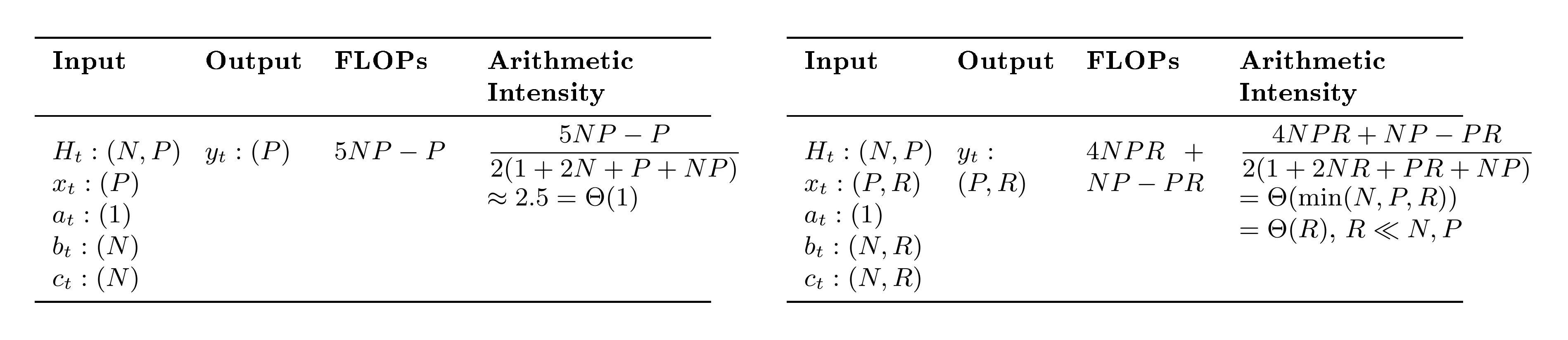
To improve hardware efficiency, we need to consider the arithmetic intensity of token generation, defined as FLOPs divided by the number of input-output bytes for a given op. Since SSM decoding saturates the memory bandwidth with idle compute (i.e., being memory-bound), we would like to increase its arithmetic intensity to effectively overlay compute with memory I/O. More concretely, the arithmetic intensity for a single generation in Mamba is around $2.5$ ops per byte (Table 2), while the arithmetic intensity for bfloat16 matmul is about $295$ ops per byte for NVIDIA H100-SXM5 ([26]). Consequently, SSM decoding falls far short of a compute-bound regime, and moreover it is not clear how one can adjust the existing parameters in Mamba to mitigate the lack of hardware efficiency. We note that this observation applies generally to other sub-quadratic models, such as causal linear attention.

From SISO to MIMO.

Consider a single head of a typical SSM with head dimension $P$, which involves stacking the SISO recurrence ${\bm{h}}t \gets \alpha_t {\bm{h}}{t-1} + \Delta_t {\bm{B}}_t x_t$ with $P$ copies sharing the same $\alpha_t, \Delta_t$ and ${\bm{B}}_t$. The resulting broadcasted recurrence ${\bm{h}}t \gets \alpha_t {\bm{h}}{t-1} + \Delta_t {\bm{B}}_t {\bm{x}}_t^\top$ takes vector inputs ${\bm{x}}_t \in \mathbb{R}^P$ and has matrix-valued states ${\bm{h}}_t \in \mathbb{R}^{N \times P}$.

Note that the memory traffic (input and output size) is dominated by the state ${\bm{h}}_t$, while the computation mainly comprises the outer product ${\bm{B}}_t {\bm{x}}_t^\top$ which has FLOPs proportional to $NP$. By increasing the dimension of the latter terms, transforming ${\bm{B}}_t \in \mathbb{R}^{N} \to {\bm{B}}_t \in \mathbb{R}^{N \times R}$ and ${\bm{x}}_t \in \mathbb{R}^{P} \to {\bm{x}}_t \in \mathbb{R}^{P \times R}$, the memory traffic does not significantly increase (for small $R$) while the FLOPs consumed increase by a factor of $R$ (Table 2). Thus, this transformation increases the arithmetic intensity of the recurrence. Furthermore, the increase in arithmetic intensity is translated into practical gains, since the outer product ${\bm{B}}_t {\bm{x}}_t^\top$ becomes a hardware-efficient matrix-matrix product (matmul), which is computed using fast tensor-cores, incurring only a marginal latency cost. As a result, the MIMO recurrence is more expressive than the original SISO recurrence, computing $R {\scriptstyle\times}$ more FLOPs while practically preserving the decoding speed.

For similar reasons, the computation of the output from the state, ${\bm{y}}_t \gets {\bm{C}}_t^\top {\bm{h}}_t$ acquires an extra rank $R$ by modifying the output projection as ${\bm{C}}_t \in \mathbb{R}^{N} \to {\bm{C}}_t \in \mathbb{R}^{N \times R}$. Overall, this transformation is equivalent to expanding the original single-input, single-output (SISO) recurrence to multi-input, multi-output (MIMO).

Training MIMO SSMs.

While the MIMO formulation is motivated by inference efficiency, the training algorithms for SSMs (including our developments in Section 3.1, Section 3.2) have been typically developed for SISO models. We begin with the observation that MIMO SSMs can be expressed in terms of $R^2$ SISO SSMs, where $R$ SISO SSMs sharing the same recurrence are summed for each of the $R$ MIMO outputs. In particular, define $ {\bm{C}}_t^{(i)} \in \mathbb{R}^N, {\bm{B}}_t^{(j)} \in \mathbb{R}^N, {\bm{x}}_t^{(j)} \in \mathbb{R}, \Delta_t \in \mathbb{R}$, where $i, j \in {0, ..., R-1}$, then we have,

$ \begin{align} {\bm{h}}t^{(j)} &\gets \alpha_t {\bm{h}}{t-1}^{(j)} + \Delta_t {\bm{B}}_t^{(j)} {\bm{x}}_t^{(j)} \tag{a}\ {\bm{h}}t &= \sum{j=0}^{R-1} {\bm{h}}_t^{(j)} \tag{b}\ {\bm{y}}_t^{(i)} &\gets \left({\bm{C}}_t^{(i)}\right)^\top {\bm{h}}_t \tag{c} \end{align}\tag{9} $

Thus, $y_t^{(i)} = \sum_j \mathsf{SSM}!\left(\alpha, \Delta, {\bm{B}}^{(j)}, {\bm{C}}^{(i)}, {\bm{x}}^{(j)}\right)_t$, where $\mathsf{SSM}!\left(\alpha, \Delta, {\bm{B}}^{(j)}, {\bm{C}}^{(i)}, {\bm{x}}^{(j)}\right)_t := \left({\bm{C}}_t^{(i)}\right)^\top {\bm{h}}_t^{(j)}$ with ${\bm{h}}_t^{(j)}$ from Equation (9a).

Furthermore, improvements to standard SISO-based SSM models can be directly applied to MIMO models as the underlying SISO training algorithms can be utilized as a black-box. This observation allows a MIMO model to be trained by invoking the SISO algorithm $R^2$ times as a black box in parallel. In contrast, when computed in the recurrent form, equation~Equation (9a), Equation (9b), and (9c) can be performed sequentially, incurring only an $R$-times overhead relative to SISO SSMs (recall the discussion on MIMO decoding FLOPs).

Chunked Algorithm for MIMO SSMs.

Many modern SISO recurrent models, including Mamba-2, are computed using a chunked algorithm, where the sequence is divided into chunks of length $C$. Within each chunk, a parallel (but asymptotically slower) algorithm is applied, while a recurrence is computed across chunks. Chunked algorithms interpolate between two extremes: a fully parallel and a fully sequential algorithm. By exploiting this structure, we can reduce the training cost of MIMO SSMs to $R$ times that of SISO SSMs. This idea also appears in the SSD framework—SSD applies a hardware-friendly quadratic algorithm within each chunk, while using the recurrent form across chunks, and shows that when the state and head dimensions are comparable, setting the chunk size to this dimension yields an overall linear-time algorithm. Specifically, SSD's intra-chunk computation incurs $\left(2C^2 N + 2C^2 P\right)$ FLOPs per chunk, giving a total of $\frac{T}{C}\left(2C^2 N + 2C^2 P \right) = 2TC(N+P)$. The inter-chunk computation incurs $4NPC + 2NP$ FLOPs per chunk, for a total of $\frac{T}{C}(4NPC + 2NP) = 4TNP + \frac{T}{C}2NP$ (ignoring negligible terms). Setting $C=P=N$, the total FLOP count is $8TN^2$, which is linear in $T$.

The chunked algorithm for SSD can be naturally generalized into MIMO SSMs. In such a case, the FLOP counts of state projection ${\bm{B}} {\bm{x}}^\top$ and state emission ${\bm{C}}^\top {\bm{h}}$ increase by $R\times$, while the FLOP count of the intrachunk component ${\bm{C}}^\top {\bm{B}}$ increases by $R^2\times$. As a result, the intra-chunk computation incurs $2 \cdot \left(\frac{T}{C} (CR)^2 N + \frac{T}{C} (CR)^2 P\right)$ FLOPs and inter-chunk computation incurs $4\cdot\frac{T}{C}NP(CR) + 2\cdot\frac{T}{C}NP$ FLOPs. Thus, setting $CR=N=P$ yields a total FLOP count of $8TRN^2$, an $R$-fold increase in FLOP count. Intuitively, setting MIMO chunk size as $\frac{1}{R}$ times the SISO chunk size, i.e., $C_{\text{MIMO}} \gets \frac{1}{R}C_{\text{SISO}}$, maintains the SISO intra-chunk FLOP count while increasing the number of chunks by a factor of $R$, resulting in an overall $R$-times increase in FLOP count instead of an $R^2$-times increase while keeping the algorithm hardware-friendly.

The training speed of algorithms in practice depends on details of the kernel implementation strategy, architectural choices such as how the MIMO parameters are instantiated, and problem dimensions, but should be no more than $R$ times slower. Our released Triton Mamba-3 SISO kernels are roughly on par with the Triton Mamba-2 kernels, and MIMO kernels only incur a slowdown of $2 {\scriptstyle\times}$ when $R=4$, as compute latency can be parallelized with memory movement. Table 6 benchmarks the prefill speed of various kernels which is equivalent to the forward pass of the training kernel.

MIMO Instantiation.

Among various choices for MIMO parameterizations, Mamba-3's approach achieves a balance that preserves the state size and number of SSMs of its SISO counterpart, while avoiding excessive growth in parameter count. The naive conversion of a SISO SSM to a rank $R$ MIMO SSM would incur an $R\times$ increase in parameters as all projections that model the inputs to the SSM, ${\bm{B}}, {\bm{C}}, {\bm{x}}$, would increase. Block-level components, such as the gate ${\bm{z}}$ (which so far has been ignored for simplicity) and output ${\bm{y}}$ projection would also be impacted. This influx in parameter count would be intractable at larger model scales. To counteract this, we make the following change. Mamba's multi-value attention (MVA) head structure results in shared ${\bm{B}}, {\bm{C}}$ across heads, so these components' projections can be directly converted to incorporate the new MIMO rank $R$ with only a slight increase in parameter count from $DN$ to $DNR$ for the entire layer (recall $D$ as the model dimension). However, the SSM input ${\bm{x}}_t$, output ${\bm{y}}_t$, and gate ${\bm{z}}_t$ are unique per head and therefore dominate the parameter count. Here, directly adjusting the projections would increase the parameter count from $DP$ to $DPR$ for each head. Instead, we keep the original SISO projection and element-wise scale each dimension of the projected output to size $R$ with a learnable, data-independent vector, resulting in $DP + PR$ parameters for each head. This mitigates the multiplicative increase to a more reasonable additive parameter count increase. Appendix C details the parameterization, and all MIMO-variants in our paper are parameter-matched to their SISO counterparts by reducing the MLP width.

Remark

For simplicity, all discussion in this section was for simpler 2-term recurrences such as that arising from exponential-Euler discretization; the generalization to the 3-term exponential-trapezoidal recurrence is similar.

3.4 Mamba-3 Architecture

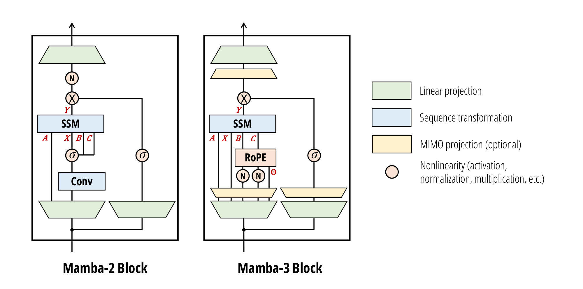
The overall architecture follows Llama~([27]), alternating Mamba-3 and SwiGLU blocks with pre-norm. The Mamba-3 block retains the overall layout of its predecessor, while introducing several key modifications.

Updated SSM Recurrence.

The SSD layer is replaced with the more expressive complex-valued exponential-trapezoidal SSM defined in Proposition 4. Mamba-3 employs the SISO SSM by default to enable fair comparisons with other SISO-like models, but its MIMO variant can be trained and deployed as a stronger alternative to baseline Mamba-3 (Table 3). Our SSM ${\bm{A}}$ is complex with both real and imaginary components produced by data-dependent projections. With Figure 2, this is partitioned into the real-valued $A$ and imaginary-valued $\Theta$; the former is passed into the SSD black box as in Mamba-2, while the latter is computed through the RoPE trick.

BC / QK Normalization.

RMS normalizations are added following the ${\bm{B}}, {\bm{C}}$ projection, mirroring the QKNorm commonly used in modern Transformers([28, 29]) and other recent linear models([30, 31]). We call this either BC normalization (BCNorm) or QK normalization (QKNorm) interchangeably. We find that BCNorm is also able to stabilize large-scale runs, resulting in the removal of the post-gate RMSNorm layer (introduced in Mamba-2 for stability) in our pure Mamba-3 models. However, in hybrid models, the removed RMSNorm layer is crucial for long-context extrapolation (Table 4).

${\bm{B}}, {\bm{C}}$ Biases.

Similarly to [32], which proved that adding channel-specific biases to ${\bm{B}}$ in a blockwise variant of Mamba-1 grants universal approximation capabilities, Mamba-3 incorporates learnable, head-specific, channel-wise biases into the ${\bm{B}}$ and ${\bm{C}}$ components after the BCNorm.

We hypothesize that these biases also induce a convolution-like behavior in the model. Specifically, adding biases to ${\bm{B}}$ and ${\bm{C}}$ introduces data-independent components into SSMs that function more similarly to convolutions. Ablations on the bias parameterization are located in Appendix F.

The combination of data-independent bias parameters, together with exponential-trapezoidal discretization (which itself induces a convolution on the state-input), is empirically able to obviate the short causal convolution and its accompanying activation function present in Mamba-2 and most modern recurrent models (Section 4.2).

4. Empirical Validation

Section Summary: The section empirically tests the Mamba-3 model, which uses state space models for efficient sequence processing, on synthetic and real-world tasks to confirm improvements over previous versions. In language modeling, Mamba-3 outperforms baselines across different model sizes when trained on a large educational text dataset, and its multi-input multi-output variant further boosts performance with only minor adjustments to other components. For retrieval tasks, like recalling information from long sequences, Mamba-3 excels in synthetic scenarios and associative recall but faces challenges with unstructured data, though hybrid versions combining it with attention mechanisms enhance overall capabilities.

We empirically validate our SSM-centric methodological changes through the Mamba-3 model on a host of synthetic and real-world tasks. Section 4.1 evaluates Mamba-3 on language modeling and retrieval-based tasks. Section 4.2 ablates the effect of our new SSM components such as discretization and complex transitions. Section 4.3 explores the inference efficiency of the Mamba-3 family and MIMO Mamba-3's benefits over the SISO variant under fixed inference compute, and Section 4.4 benchmarks the performance of our Mamba-3 training and inference kernels.

4.1 Language Modeling

All models are pretrained with 100B tokens of the FineWeb-Edu dataset([33]) with the Llama-3.1 tokenizer([27]) at a 2K context length with the same standard training protocol. Training and evaluation details can be found in Appendix D.

Across all four model scales, Mamba-3 outperforms popular baselines at various downstream tasks (Table 3). We highlight that Mamba-3 does not utilize the external short convolution that has been empirically identified as an important component in many performant linear models~([15, 30, 34]).

4.1.1 MIMO

We aim to further verify the gain from MIMO by investigating its language-modeling capabilities by training MIMO models with rank $R=4$ under the same settings. To ensure that the total parameter count is comparable to SISO-based models, we decrease the inner dimension of the MLP layers in MIMO models to compensate for the increase due to the MIMO projections. In the 1.5B-parameter models, for instance, the MLP inner dimension is reduced by only $6.6%$, from 4096 to 3824. See Appendix C for more details.

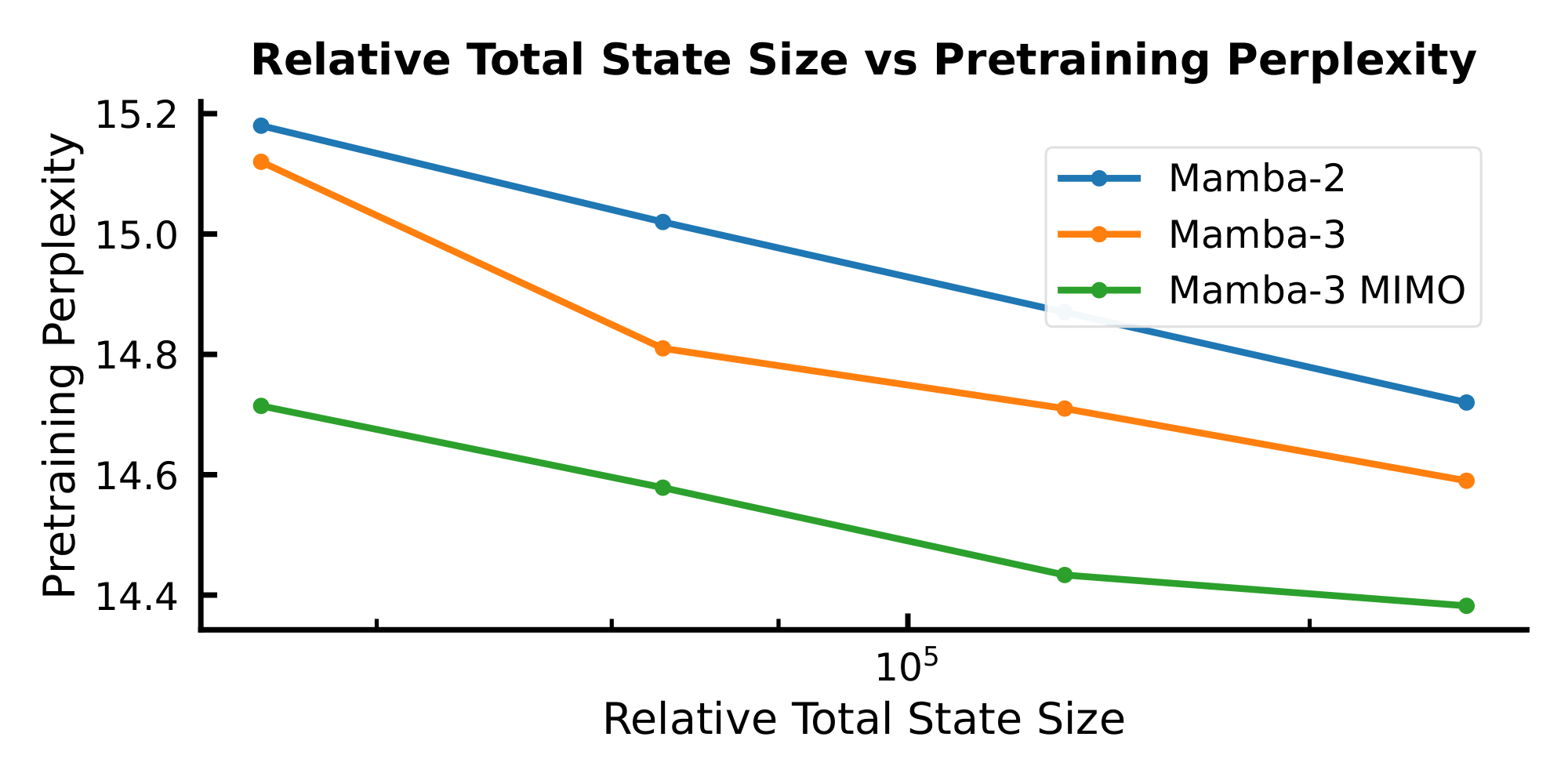
On both validation perplexity and our suite of language evaluation tasks (Table 3), we see significant gains when moving from SISO to MIMO for our Mamba-3 models. Namely, we achieve a significant perplexity gain of $0.11$ on the 1.5B models, and Figure 3 illustrates the downward shift in our validation loss. On the language evaluation front, we see gains on most tasks when compared to SISO, resulting in an average gain of 1.2 percentage points over SISO.

4.1.2 Retrieval Capabilities

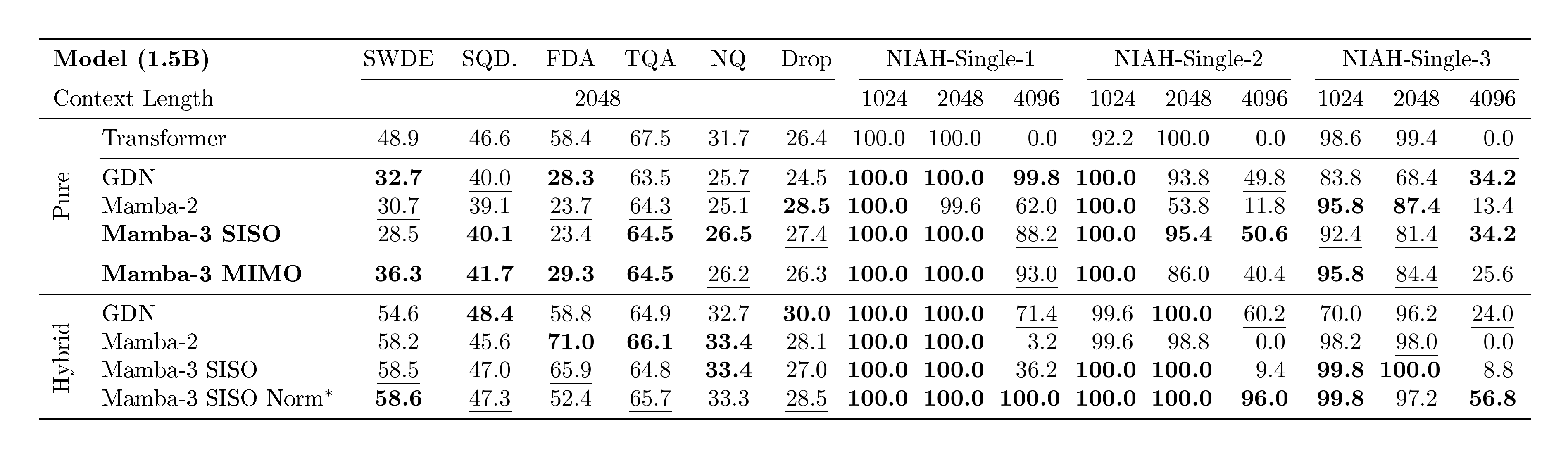
Beyond standard language modeling, an important measure for linear models is their retrieval ability—how well they can recall information from earlier in the sequence([35, 36]). Unlike attention models, which can freely revisit past context with the growing KV cache, linear models must compress context into a fixed-size state. This trade-off is reflected in the Transformer baseline's substantially stronger retrieval scores. To evaluate Mamba-3 under this lens, Table 4 compares it against baselines on both real-world and synthetic needle-in-a-haystack (NIAH) tasks([37]), using our pretrained 1.5B models from Section 4.1. We restrict the task sequence length to 2K tokens to match the training setup and adopt the cloze-style format for our real-world tasks to mirror the next-token-prediction objective, following [36, 38].

Mamba-3 is competitive on real-world associative recall and question-answering (TQA, SQuAD) but struggles when extracting information from semi-structured or unstructured data (SWDE, FDA). On synthetic NIAH tasks, however, Mamba-3 surpasses or matches baselines on most cases and notably demonstrates markedly better out-of-distribution retrieval abilities than its Mamba-2 predecessor.

Improving Retrieval with Hybrid Models.

Because of the natural retrieval-based weaknesses of fixed state-size, we predict that linear layers will be predominantly used in hybrid architectures that mitigate this downside with quadratic self-attention layers. To evaluate how Mamba-3 performs within this architectural paradigm, we train our hybrid models at the same scale in an interleaving fashion with a 5:1 ratio of linear layer to NoPE self-attention([39]). As seen in prior work([40]), hybrid models outperform the Transformer baseline. We find that the reintroduction of the pre-output projection RMSNorm (pre-gate, grouped RMSNorm in Table 4) to the Mamba-3 layer improves the length generalization retrieval abilities at the slight cost of in-context, real-world retrieval tasks and is highly competitive as a linear sequence mixing backbone when mixed with self-attention. However, the ideal norm type (grouped vs default) and its placement (pre- vs post-gate) is still unclear due to competing tradeoffs (Appendix E, Table 9), as we find that hybrid models and their exact characteristics and dynamics are complex and oftentimes unintuitive, a point echoed in recent works such as [41].

4.2 SSM Methodology Ablations

Table 5 ablates the changes that Mamba-3 introduces to core SSM components, mainly the introduction of BC bias and exponential-trapezoidal discretization. We report the pretraining test perplexity on models at the 440M scale, trained for Chinchilla optimal tokens. We find that the bias and exponential-trapezoidal SSM synergize well and make the short convolution utilized by many current linear models redundant.

We empirically demonstrate that data-dependent RoPE in Mamba-3 enables state tracking. Following [16], we evaluate on tasks from the Chomsky hierarchy—Parity, Modular Arithmetic (without brackets), and Modular Arithmetic (with brackets)—and report scaled accuracies in Table 5. Mamba-3 solves Parity and Modular Arithmetic (without brackets), and nearly closes the accuracy gap on Modular Arithmetic (with brackets). In contrast, Mamba-3 without RoPE, Mamba-3 with standard RoPE~([18]), and Mamba-2 fail to learn these tasks. We use the state-tracking-enabled variant of GDN and observe that Mamba-3 is competitive—matching parity and approaching its performance on both modular-arithmetic tasks. Experimental settings are covered in Appendix D.

4.3 Inference Efficiency to Performance Tradeoff

\begin{tabular}{l*{2}{S[table-format=1.3]}*{2}{S[table-format=1.3]}}
          \toprule
          \multirow{2}{*}{\textbf{Model}}
          & \multicolumn{2}{c}{\textbf{FP32}}
          & \multicolumn{2}{c}{\textbf{BF16}} \\
          \cmidrule(lr){2-3} \cmidrule(lr){4-5}
          & {$d_{\text{state}}=64$} & {$d_{\text{state}}=128$}
          & {$d_{\text{state}}=64$} & {$d_{\text{state}}=128$} \\
          \midrule
          Mamba-2        & 0.295 & 0.409 & 0.127 & 0.203 \\
          GDN & 0.344 & 0.423 & 0.176 & 0.257 \\
          Mamba-3 (SISO) & 0.310 & 0.399 & 0.110 & 0.156 \\
          Mamba-3 (MIMO) & 0.333 & 0.431 & 0.137 & 0.179 \\
          \bottomrule
        \end{tabular}

As $d_\text{state}$ governs the decode runtime for the sub-quadratic models considered in this paper (Section 3.3), we use it as a proxy for inference speed. By plotting the validation perplexity (a proxy for model performance) as a function of $d_\text{state}$, we aim to formulate a holistic picture about how sub-quadratic models can trade off performance with inference speed.

Figure 3 shows such a Pareto frontier for the Mamba models considered in this paper. For each data point, we train a 440M parameter model to $2\times$ Chinchilla optimal tokens on the Fineweb-Edu dataset, where the model is configured with a $d_\text{state}$ of ${16, 32, 64, 128}$. As expected, we observe an inverse correlation between validation loss and $d_\text{state}$. Moreover, there is a general downward shift on the Pareto frontier moving from Mamba-2 to Mamba-3, indicating a stronger model: in this setting, Mamba-3 with $2\times$ smaller state size achieves better pretraining perplexity than its Mamba-2 counterpart, resulting in a faster model with the same quality or a better model for the same speed.

A further downward shift is observed when moving from the SISO variant of Mamba-3 to the MIMO variant of Mamba-3 (where we set the MIMO rank $R = 4$ and decrease the MLP inner dimension to parameter match the SISO variants).

We expand the comparison to include the GDN baseline in Appendix E, Figure 7, which also shows Mamba-3 comparing favorably to GDN.

4.4 Fast Mamba-3 Kernels

We complement Mamba-3's methodological advances with optimized kernels that deliver fast inference in practical settings. We implement a new series of inference kernels for Mamba-3—using Triton for the forward (prefill) path and CuTe DSL for decode—and compare their per-token decode latency against the released Triton kernels for Mamba-2 and GDN in Table 6.[^4] The evaluation measures a single decode step at batch size 128 on a single H100 for both FP32 and BF16 datatypes; models are 1.5B parameters with model dimension $2048$ and state dimension $\in {64, 128}$. Across all configurations, SISO achieves the lowest latency amongst baselines. MIMO, with its higher arithmetic intensity, increases the decoding FLOPs without significantly increasing decode runtime. Our benchmarks indicate that our CuTe DSL decode implementation is competitive and that the additional components of Mamba-3 (exponential-trapezoidal update, complex-valued state, and MIMO projections) are lightweight. This supports our overall inference-first perspective: Mamba-3 admits a simple, low-latency implementation while providing strong empirical performance.

[^4]: Details on each kernel DSL and the exact kernel fusion structure is provided in Appendix G.

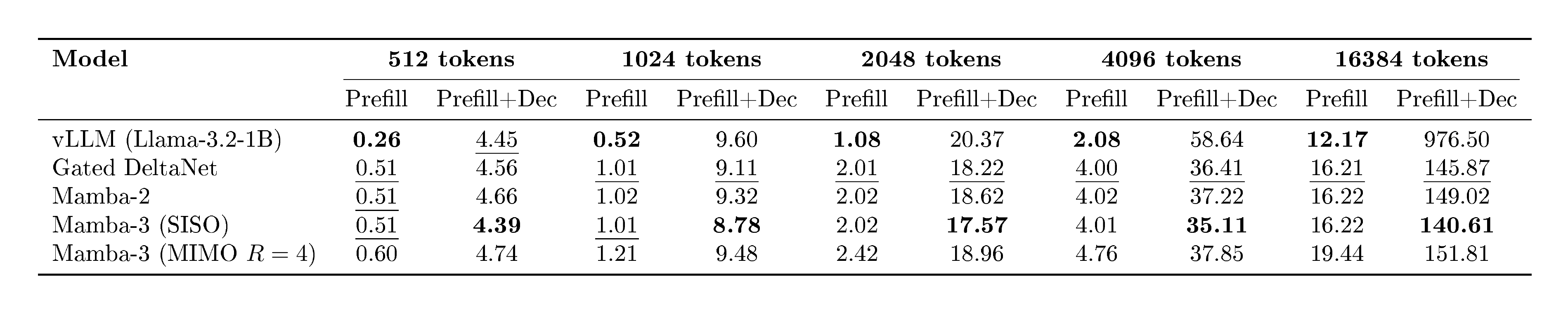
Table 7 benchmarks both end-to-end latency across different decoding sequence length and prefill time for the same sequence length. The decode time is consistent with Table 6, where Mamba-3 (SISO) is fastest; Mamba-3 (MIMO) is on par with Mamba-2; and all linear methods are faster than optimized attention as sequence length grows. We also see that MIMO incurs a moderate overhead for prefill, as discussed in Section 3.3. Details of the benchmark are in Appendix G.

5. Related Work

Section Summary: Researchers are developing faster ways to process sequences of data, like text, by replacing the slow attention mechanism in AI models with linear-time alternatives, including linear attention approximations, test-time training that updates models on the fly, and state space models inspired by signal processing, with recent advances like Mamba-2 linking them closely to attention. Studies highlight limitations in how these models track and represent complex information, leading to enhancements such as complex-valued parameters for better expressivity, especially in Mamba-3, which uses rotational embeddings to handle language tasks more effectively. Efforts have also shifted between single-input single-output designs, which offer larger memory but are computationally heavy, and multi-input multi-output versions that simplify processing while balancing capacity and speed.

5.1 Linear-Time Sequence Mixers

A growing body of work seeks to replace the quadratic softmax-based attention mechanism~([7, 42]) with linear runtime alternatives. Prominent approaches can be categorized under three broad frameworks: linear attention, test-time training, and state space models.

Many nascent linear attention (LA) models aimed to approximate softmax attention through kernel feature maps([19, 43]), while recent models have discarded the feature maps for raw dot-products between queries and keys, modulated by decays or masks([44, 45]). More recently, fast-weight programmers [9] that modulate the state memory with key-value pairs have also fallen under the umbrella term "linear attention." [30, 10] originated from this line of work and enhanced traditional linear attention by replacing the additive memory update with a delta-rule recurrence. This has further spurred on a host of work improving the efficiency and capabilities of linear models built on the delta rule~([13, 31]).

A parallel line of test-time training (TTT) or test-time regression (TTR) work views sequence modeling as an online learning task during inference. Here, the recurrent state represents a compressed summary of past inputs, and recurrent steps update the state to memorize new information([46, 47, 48]). Equivalently, these methods can be viewed as optimization of a global regression objective, and recurrent state updates represent iterative optimization procedures such as variants of gradient descent([49]).

Structured state space models (SSMs) are another view of modern recurrent models inspired by classical signal processing and dynamical systems. Early versions of SSMs such as S4([20, 22, 50]) used linear time invariant (LTI) layers with structured state transition matrices, for example diagonal or low-rank plus diagonal, to facilitate efficient computation and stable learning of long-context tasks([20, 22, 50]). The introduction of time-varying, input-dependent selectivity to SSMs in Mamba-1 ([15]) reduced the disparity between self-attention and linear models on information-dense modalities, notably language modeling. Subsequently, Mamba-2 ([8]) formalized the connection between SSMs and (linear) attention through the structured state space duality (SSD) that we build on in this work.

5.2 State Tracking and Complex State Space Models

Expressivity and State Tracking.

Recent work characterizes the types of state that recurrent, constant-memory mixers can maintain, revealing algorithmic deficiencies in previous SSM-based models. [24] show that under finite precision, practical SSMs collapse to $\mathrm{TC}^0$, leading to failures on tasks like permutation composition over $S_5$ unless the primitive is extended. Similarly, [32] prove that a single-layer Mamba is not a universal approximator. Several modifications have been proposed to improve expressivity. For instance, the same work shows that a block-biased variant regains the universal approximation property with only minor changes, either through block decomposition or a channel-specific bias. Allowing negative eigenvalues or non-triangular transitions enables linear RNNs—including diagonal and Householder/DeltaNet forms—to capture parity and, under mild assumptions, regular languages ([16]). Complex-valued parameterizations provide another avenue for enhanced expressivity.

Complex State Space Models.

Structured SSMs prior to Mamba were frequently complex-valued, rooted in traditional SSM theory. They also generally excelled in domains such as vision and audio, which have explicit frequency-based information content, rather than language. While some models such as H3([51]), RetNet([44]), and Megalodon~([52]) kept complex-valued SSMs while targeting language modeling, they still noticeably underperformed Transformers.

Additionally, because these models were LTI and were computed using very different algorithms (in particular, convolutions or explicit recurrence) than modern selective SSMs such as Mamba, they generally did not use the RoPE trick to handle the complex part. An exception is RetNet, which introduced a model in between linear attention and Mamba-2 that used constant scalar decays (as opposed to no decay in LA and data-dependent decay in Mamba-2) with an additional constant complex phase that was implemented through RoPE.

In general, complex numbers have been empirically found to be unhelpful for language modeling, and hence were phased out in Mamba-1 and successors, including parallel lines of work on linear attention and test-time training. Mamba-3 represents the first modern recurrent model with complex-valued state transitions, which were introduced for specific purposes of increasing expressivity and state-tracking ability. By incorporating the RoPE trick, this represents, to the best of our knowledge, the first usage of data-dependent RoPE grounded in theoretical motivations.

5.3 Multi-Input, Multi-Output

S4([20]) is a single-input, single-output LTI system where each dimension of the input was assigned its own independent SSM. Such SISO models have a significantly larger recurrent state than classical RNNs, and necessitated more complicated mathematical machinery to compute them efficiently. Aiming to simplify the model, S5([22]) and LRU([53]) replaced the set of SISO SSMs with a multi-input, multi-output SSM applied directly on the entire vectorized input. This change reduced the effective state capacity but enabled an alternate computation path by directly computing the recurrence with a parallel scan. While this trade-off between state capacity and modeling performance was less pronounced in LTI models, Mamba-1 (S6)([15]) and Mamba-2~([8]) returned to the SISO system due to the importance of a large state size in the time-varying setting. The computational bottleneck associated with the increased state size was addressed with a hardware-aware parallel scan algorithm for Mamba-1 and a matrix multiplication-based algorithm for Mamba-2.

The introduction of MIMO to Mamba-3 significantly diverges from prior work. Unlike previous MIMO models, which aimed to simplify training algorithms at the cost of slightly reduced expressivity, Mamba-3's MIMO structure is motivated to increase modeling power while preserving inference efficiency. Accordingly, its state expansion is kept at Mamba-1/-2 levels to maintain modeling capabilities while trading off additional training compute.

5.4 The State Space Model Viewpoint

Although modern recurrent models have several different viewpoints that largely converge (Section 5.1), each framework has slightly different interpretations and motivations that can lead to different design spaces and extensions. In particular, linear attention and test-time training are more closely related and can perhaps be lumped together under a framework of associative memory that explicitly aims to memorize input data through "key-value" stores; either through approximations to the canonical KV method (i.e., quadratic attention) in LA, or by minimizing soft optimization objectives in TTT. On the other hand, state space models have a different lineage, as reflected both in terminology (e.g., $A, B, C, X$ instead of $Q, K, V$) and in their natural extensions. Notably, the methodological improvements in Mamba-3 are all associated with the SSM viewpoint specifically and are less motivated from associative memory frameworks.

1. Exponential-Trapezoidal Discretization. The SSM viewpoint entails the discretization of a continuous ODE governing the system; our exponential-trapezoidal discretization falls out of an improved discretization method. As associative memory methods do not use discretization, it is not obvious how to interpret a 3-term recurrence such as exponential-trapezoidal under alternate viewpoints.
2. Complex-Valued State Transitions. Complex SSMs have long been a staple of dynamical systems, and it is natural to consider complex values as an extension of selective SSMs. On the other hand, the associative memory framework interprets the $A$ state transition as a coefficient of an objective function, for example corresponding to the weight of an L2 regularization (or weight-decay) term in the optimization objective ([49]). However, complex values are meaningless as the coefficient of a regression objective; hence, Mamba-3 is not obviously interpretable within these frameworks.
3. Multi-Input, Multi-Output. MIMO is a classical concept from the state space model literature and does not naturally appear in associative memory (linear attention or test-time training) frameworks. However, we do note that the MIMO formulation introduced in this paper is not directly tied to SSM theory—and instead is motivated from a computational perspective—and our techniques can be adapted to other modern recurrent models as well.

There continues to be vigorous progress in the development of linear-time sequence models, and the discussion here only captures a portion of them. We anticipate a growing space of unified frameworks, improved understanding, and new generalizations as the development of these models continually evolves.

6. Conclusion And Future Work

Section Summary: Mamba-3 is a new AI model designed for processing sequences like text, featuring upgrades that make it more effective and efficient than earlier versions, such as better ways to handle patterns and a setup that boosts its ability to model complex data. Its simpler form performs strongly in language tasks on its own or combined with other models, pushing the balance between speed and accuracy further ahead. An advanced version trades longer training time for even greater power while keeping quick performance during use, overall offering straightforward improvements and fresh ideas for building efficient sequence-handling AI.

We introduce Mamba-3, a state space model with several methodological improvements over prior SSMs: a more powerful recurrence via exponential-trapezoidal discretization; improved expressivity through complex-valued state transitions; and higher inference efficiency and modeling abilities with a MIMO formulation. The base SISO version of Mamba-3 delivers strong language modeling results, both standalone and in interleaved hybrid architectures, and advances the Pareto frontier on the performance-efficiency tradeoff over prior linear sequence models. The MIMO version trades off slower training for even stronger modeling power, while maintaining competitive inference efficiency compared to Mamba-2. Put together, the techniques in Mamba-3 show simple and theoretically motivated improvements from the state space model viewpoint, and open up new directions and design principles for efficient sequence models.

Acknowledgments.

We gratefully acknowledge the support of the Schmidt Sciences AI2050 fellowship, the Google ML and Systems Junior Faculty Awards, the Google Research Scholar program, Princeton Language and Intelligence (PLI), Together AI, and Cartesia AI. KL is supported by the NSF GRFP under Grant DGE2140739. We also thank Sukjun Hwang and Gaurav Ghosal for helpful feedback and discussions.

Appendix

Section Summary: The appendix describes a method for approximating how a linear state-space model evolves over continuous time by breaking it into discrete time steps, using exponential functions to handle decay and trapezoidal rules to integrate inputs, which keeps errors small—on the order of the square or cube of the time step size. It includes a proof showing how this works by applying an integrating factor to simplify the math and rearrange the equations. Further sections detail how this approximation fits into computational structures like mask matrices in models such as Mamba-2 and analyze the precise error rates under standard smoothness assumptions.

A. Exponential-Trapezoidal Discretization

Proposition 5: Variation of Constants~([54])

Consider the linear SSM

$ \dot{{\bm{h}}}(t) = A(t), {\bm{h}}(t) + {\bm{B}}(t), x(t), $

where ${\bm{h}}(t)\in\mathbb{R}^N$, $A(t)\in\mathbb{R}$ is a scalar decay, and ${\bm{B}}(t)x(t)\in\mathbb{R}^N$.

For $\Delta_t$ discretized time grid $\tau_t = \tau_{t-1} + \Delta_t$, the hidden state satisfies equation (10aa), which can then be approximated to equation (10ab) with $O(\Delta_t^2)$ error.

The approximation of the remaining integral on the state-input can have varying error bounds depending on the method used: an example can be found in Appendix A.2.

$ \begin{align} \tag{a} {\bm{h}}(\tau_t) &= \exp!\left(\int_{\tau_{t-1}}^{\tau_t} A(s), ds\right){\bm{h}}(\tau_{t-1})

• \int_{\tau_{t-1}}^{\tau_t} \exp!\left(\int_{\tau}^{\tau_t} A(s), ds\right){\bm{B}}(\tau)x(\tau), d\tau, \ \tag{b} {\bm{h}}t &\approx e^{\Delta_t A_t}, {\bm{h}}{t-1}
• \int_{\tau_{t-1}}^{\tau_t} e^{(\tau_t-\tau)A_t}, {\bm{B}}(\tau)x(\tau), d\tau . \end{align}\tag{10} $

Proof.: Starting from the initial linear SSM, an integrating factor $z(t) \coloneqq e^{\int^t_0 -A(s)ds}$ is applied to facilitate integration.

$ z(t) \dot{{\bm{h}}}(t) = z(t)A(t){\bm{h}}(t) +z(t){\bm{B}}(t)x(t) $

Considering $z'(t) = -A(t)z(t)$; through rearranging the terms and integrating between the time grid $[\tau_{t-1}, \tau_t]$

$ \int_{\tau_{t-1}}^{\tau_t} \frac{d}{d\tau}\left(z(\tau) {\bm{h}}(\tau) \right) d\tau = \int_{\tau_{t-1}}^{\tau_t} z(\tau) {\bm{B}}(\tau)x(\tau) d\tau $

results in

$ z(\tau_t){\bm{h}}(\tau_t) - z(\tau_{t-1}){\bm{h}}(\tau_{t-1}) = \int_{\tau_{t-1}}^{\tau_t} z(\tau){\bm{B}}(\tau)x(\tau) d\tau, $

which can be arranged in a more familiar form

$ {\bm{h}}(\tau_t) = z(\tau_t)^{-1}z(\tau_{t-1}){\bm{h}}(\tau_{t-1}) + \int_{\tau_{t-1}}^{\tau_t} z(\tau_t)^{-1}z(\tau){\bm{B}}(\tau)x(\tau) d\tau. $

Substituting the integrating factor $z(\tau)$ corresponds to

$ {\bm{h}}(\tau_t) = \exp\left(\int_{\tau_{t-1}}^{\tau_t}A(s)ds\right){\bm{h}}(\tau_{t-1}) + \int_{\tau_{t-1}}^{\tau_t} \exp\left(\int_{\tau}^{\tau_t}A(s)ds\right){\bm{B}}(\tau)x(\tau) d\tau. $

We approximate the state-transition integral with a right-hand assumption where $\forall s \in [\tau_{t-1}, \tau_t], A(s) \coloneqq A(\tau_t)$ which we refer to as $A_t$,

$ {\bm{h}}t \approx \underbrace{\exp\left(\Delta_t A_t\right){\bm{h}}{t-1}}\text{right-hand approximation} + \underbrace{\int{\tau_{t-1}}^{\tau_t} \exp\left((\tau_t -\tau)A_t\right){\bm{B}}(\tau)x(\tau) d\tau}_\text{to be approximated}. $

incurring a local truncation error of order $O(\Delta_t^2)$. Thus, we have approximated the exponential dynamics of the adjusted underlying ODE and leave the state-input integral to be approximated with any host of methods.

A.1 Exponential-Trapezoidal Discretization's Mask Matrix

Proof: When viewing the tensor contraction form, let us call $C = (T, N), B=(S, N), L=(T, S), X=(S, P)$ based on the Mamba-2 paper. With this decomposition of our mask, we can view $L = \text{contract}(TZ, ZS\rightarrow TS)(L_1, L_2)$.

The original contraction can be seen as

$ \text{contract}(TN, SN, TS, SP\rightarrow TP)(C, B, L, X) $

We can now view it as

$ \text{contract}(TN, SN, TJ, JS, SP\rightarrow TP)(C, B, L_1, L_2, X) $

This can be broken into the following:

$ \begin{align*} Z &= \text{contract}(SN, SP\rightarrow SNP)(B, X)\ Z' &= \text{contract}(JS, SNP\rightarrow JNP)(L_2, Z)\ H &= \text{contract}(TJ, JNP\rightarrow TNP)(L_1, Z') \ Y &= \text{contract}(TN, TNP\rightarrow TP)(C, H) \end{align*} $

We can view this step: $\text{contract}(ZS, SNP\rightarrow ZNP)(L_2, Z)$ as a convolution of size two applied on the state-input ($B, X$ outer product) prior to the decay with the traditional SSD $L=L_1$ matrix.

A.2 Exponential-Trapezoidal Discretization Error Rate

Standard assumptions.

We assume that: $A(t), {\bm{B}}(t), x(t)$ are bounded and $C^3$ on each timestep, so that $g(\tau)$ has three bounded derivatives; the map ${\bm{h}} \mapsto A(t){\bm{h}} + {\bm{B}}(t)x(t)$ is Lipschitz in ${\bm{h}}$ which is true for linear systems; $\lambda_t$ lies in a bounded interval so that the update is zero-stable.

Proof: Let ${\bm{g}}(\tau) \coloneqq e^{(t_k-\tau) A_k}, {\bm{B}}(\tau)x(\tau)$ denote the integrand in the second term of Proposition 5. Since $A(t), {\bm{B}}(t), x(t)$ are $C^3$ on $[t_{k-1}, t_k]$, the function $g$ has three bounded derivatives. A second-order Taylor expansion of $g$ around $t_{k-1}$ gives us,

$ \begin{align*} \int_{t_{k-1}}^{t_k} g(\tau), d\tau

\Delta_t, g(t_{k-1})

• \frac{\Delta_t^2}{2}, g'(t_{k-1})
• \frac{\Delta_t^3}{6}, g''(t_{k-1})
• O(\Delta_t^4). \end{align*} $

Recall that the trapezoidal approximation to this integral is given by,

$ \begin{align*} Q_\lambda

\Delta_t \Big[(1-\lambda_t), g(t_{k-1})

• \lambda_t, g(t_k)\Big]. \end{align*} $

Expanding $g(t_k)$ using Taylor expansion: $g(t_k) = g(t_{k-1}) + \Delta_t g'(t_{k-1}) + \frac{\Delta_t^2}{2} g''(t_{k-1}) + O(\Delta_t^3)$. Substituting this into $Q_\lambda$,

$ \begin{align*} Q_\lambda &= \Delta_t\Big[(1-\lambda_t) g(t_{k-1})

• \lambda_t g(t_k)\Big] \ &= \Delta_t g(t_{k-1})
• \lambda_t \Delta_t^2 g'(t_{k-1})
• \lambda_t \frac{\Delta_t^3}{2} g''(t_{k-1})
• O(\Delta_t^4). \end{align*} $

Hence, the error is given by:

$ \begin{align*} \int_{t_{k-1}}^{t_k} g(\tau), d\tau - Q_\lambda &= \Big(\tfrac{1}{2} - \lambda_t\Big)\Delta_t^2 g'(t_{k-1})

• \Big(\tfrac{1}{6} - \tfrac{\lambda_t}{2}\Big)\Delta_t^3 g''(t_{k-1})
• O(\Delta_t^4). \end{align*} $

Under the assumption that $\lambda_t = \tfrac{1}{2} + c_t \Delta_t$, where $c_t = O(1)$, then $\tfrac{1}{2} - \lambda_t = -c_t \Delta_t = O(\Delta_t)$ and thus the $\Delta_t^2$ term is $O(\Delta_t^3)$. Therefore,

$ \begin{align*} \int_{t_{k-1}}^{t_k} g(\tau), d\tau - Q_\lambda = O(\Delta_t^3), \end{align*} $

which yields an $O(\Delta_t^3)$ local truncation error.

A.3 Exponential-Trapezoidal Parameterization

::: {caption="Table 8: Ablations on $\lambda_t$ parameterization in the exponential-trapezoidal update."}

:::

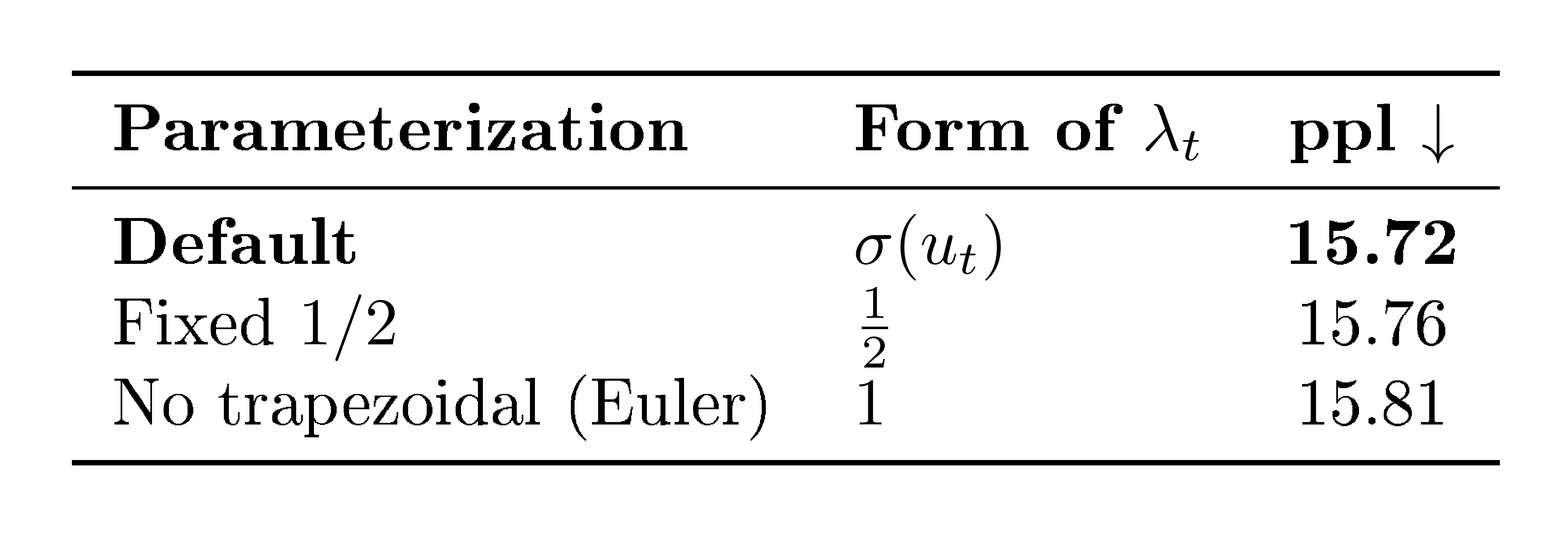
Setting: All runs use the Mamba-3 (SISO) 440M model trained at Chinchilla scale, with the other architectural and optimization hyperparameters being the same as in Table 3.

The default model uses a data-dependent gate $\lambda_t = \sigma(u_t)$, where $u_t$ is a learned projection of the current input token. In Table 8, we try different parameterizations for $\lambda_t$ and find that the default parameterization empirically performs the best. Hence, we choose the simpler default parameterization that does not enforce $\lambda_t = \tfrac{1}{2}+ O(\Delta_t)$ .

B. Complex SSM Proofs

B.1 Proof of Proposition 2

Proof.: We first present the derivation for $N=2$; the block-diagonal structure for general even $N$ follows by grouping pairs of coordinates.

Let $h_t + i\hat{h}t$ denote the complexified hidden state, with parameters $A(t)+i\theta(t)$ and $B(t)+i\hat{B}(t)$ for the transition and input, respectively. By the variation of constants formula (Proposition 5), applying zero-order hold and Euler's rule over a step $[t{k-1}, t_k]$ gives

$ h_k + i\hat{h}k = e^{\Delta_t (A_t + i\theta_t)}(h{k-1}+ i\hat{h}_{k-1})

• \Delta_t (B_t + i\hat{B}_t)x_t. $

Expanding the exponential,

$ e^{\Delta_t(A_t+i\theta_t)} = e^{\Delta_t A_t}\Big(\cos(\Delta_t\theta_t)+i\sin(\Delta_t\theta_t)\Big), $

so in real coordinates ${\bm{h}}_t=\begin{bmatrix}h_t \ \hat{h}_t\end{bmatrix}\in\mathbb{R}^2$ the recurrence becomes

$ {\bm{h}}t = e^{\Delta_t A_t} \underbrace{\begin{bmatrix} \cos(\Delta_t\theta_t) & -\sin(\Delta_t\theta_t) \ \sin(\Delta_t\theta_t) & \cos(\Delta_t\theta_t) \end{bmatrix}}{R(\Delta_t\theta_t)} {\bm{h}}_{t-1}

• \Delta_t \begin{bmatrix} B_t \ \hat{B}_t \end{bmatrix}x_t. $

Stacking across $N/2$ such pairs yields the block-diagonal transition

$ {\bm{h}}t = e^{\Delta_t A_t}, \mathrm{Block}\big({R(\Delta_t\theta_t[i])}{i=1}^{N/2}\big){\bm{h}}_{t-1}

• \Delta_t\begin{bmatrix}{\bm{B}}_t \ \hat{{\bm{B}}}_t\end{bmatrix}x_t. $

For the output,

$ y_t = \mathrm{Re}\Big(({\bm{C}}_t+i\hat{{\bm{C}}}_t)^\top(h_t+i\hat{h}_t)\Big) = \begin{bmatrix}{\bm{C}}_t \ -\hat{{\bm{C}}}_t\end{bmatrix}^\top {\bm{h}}_t, $

which defines the real projection ${\bm{C}}_t\in\mathbb{R}^N$ in the proposition. This proves the equivalence between complex SSM and the real block-diagonal system with rotations.

B.2 Proof of Proposition 3

Proof.: Consider the SSM

$ {\bm{h}}_t ;=; e^{\Delta_t A_t}, {\bm{R}}t, {\bm{h}}{t-1} ;+; \Delta_t {\bm{B}}_t x_t, \qquad y_t ;=; {\bm{C}}_t^\top {\bm{h}}_t, $

where (as in Proposition 3) $A_t\in\mathbb{R}$ is a scalar (so that $e^{\Delta_t A_t}$ is a scalar and commutes with rotations), and ${\bm{R}}_t$ is block-diagonal orthogonal/unitary, hence ${\bm{R}}_t^{-1}= {\bm{R}}_t^\top$ and the matrices ${\bm{R}}_i, {\bm{R}}_j$ commute, i.e. ${\bm{R}}_i {\bm{R}}_j= {\bm{R}}_j {\bm{R}}_i$.

Unrolling the recurrence with the convention that an empty product is the identity,

$ {\bm{h}}t ;=; \sum{i=0}^{t} \bigg(\prod_{s=i+1}^{t} e^{\Delta_s A_s}{\bm{R}}_s\bigg), \Delta_i {\bm{B}}_i x_i. $

Thus

$ \begin{align} y_t ;=; {\bm{C}}_t^\top {\bm{h}}t ;=; \sum{i=0}^{t} {\bm{C}}t^\top \bigg(\prod{s=i+1}^{t} e^{\Delta_s A_s}{\bm{R}}_s\bigg)\Delta_i {\bm{B}}_i x_i. \end{align} $

Using its unitary property,

$ \begin{align*} \prod_{s=i+1}^{t}{\bm{R}}s = \left(\prod{s=0}^{t}{\bm{R}}s\right)\left(\prod{s=0}^{i}{\bm{R}}s\right)^{-1} = \left(\prod{s=0}^{t}{\bm{R}}s\right)\left(\prod{s=0}^{i}{\bm{R}}_s^\top\right). \end{align*} $

Since $e^{\Delta_s A_s}$ are scalars, they commute with rotations; hence

$ \begin{align} y_t &= \sum_{i=0}^{t} {\bm{C}}t^\top \left(\prod{s=0}^{t}{\bm{R}}s\right) \left(\prod{s=i+1}^{t} e^{\Delta_s A_s}\right) \left(\prod_{s=0}^{i}{\bm{R}}s^\top\right) \Delta_i {\bm{B}}i x_i \ &= \left[\left(\prod{s=0}^{t}{\bm{R}}s^\top\right){\bm{C}}t\right]^\top \sum{i=0}^{t} \left(\prod{s=i+1}^{t} e^{\Delta_s A_s}\right) \left(\prod{s=0}^{i}{\bm{R}}_s^\top\right)\Delta_i {\bm{B}}_i x_i. \end{align} $

Define the rotated parameters $\overline{{\bm{C}}}t := \left(\prod{s=0}^{t}{\bm{R}}_s^\top\right){\bm{C}}_t$ and $\overline{{\bm{B}}}i := \left(\prod{s=0}^{i}{\bm{R}}_s^\top\right){\bm{B}}_i.$ Then,

$ y_t ;=; \overline{{\bm{C}}}t^\top \sum{i=0}^{t} \left(\prod_{s=i+1}^{t} e^{\Delta_s A_s}\right)\Delta_i \overline{{\bm{B}}}_i x_i. $

Equivalently, introducing the rotated state $\tilde{{\bm{h}}}t := \left(\prod{s=0}^{t}{\bm{R}}_s^\top\right){\bm{h}}_t$,

$ \tilde{{\bm{h}}}t ;=; e^{\Delta_t A_t}, \tilde{{\bm{h}}}{t-1} ;+; \Delta_t \overline{{\bm{B}}}_t x_t, \qquad y_t ;=; \overline{{\bm{C}}}_t^\top \tilde{{\bm{h}}}_t, $

B.3 Proof of Proposition 4

Proof.: We begin from the complex SSM (as in Prop. Proposition 2)

$ \begin{align*} \dot{{\bm{h}}}(t) &= \mathrm{Diag}, \left(A(t)+i\boldsymbol{\theta}(t)\right), {\bm{h}}(t) ;+;\left({\bm{B}}(t)+i\hat{{\bm{B}}}(t)\right), x(t), \ y(t) &= \mathrm{Re}, \left(({\bm{C}}(t)+i\hat{{\bm{C}}}(t))^\top {\bm{h}}(t)\right), \end{align*} $

where $A(t)\in\mathbb{R}$ is a scalar and $\boldsymbol{\theta}(t), {\bm{B}}(t), \hat{{\bm{B}}}(t), {\bm{C}}(t), \hat{{\bm{C}}}(t)\in\mathbb{R}^{N/2}$.

Recall from Prop. Proposition 5,

$ \begin{align*} {\bm{h}}t &\approx e^{\Delta_t(A_t+i\boldsymbol{\theta}t)}, {\bm{h}}{t-1} ;+; \int{\tau_{t-1}}^{\tau_t} e^{(\tau_t-\tau)(A_t+i\boldsymbol{\theta}_t)} \left({\bm{B}}(\tau)+i\hat{{\bm{B}}}(\tau)\right), x(\tau), d\tau. \end{align*} $

Applying Prop. Proposition 1 to the above integral, we get

$ \begin{align} {\bm{h}}t &= e^{\Delta_t(A_t+i\boldsymbol{\theta}t)}, {\bm{h}}{t-1} ;+; \beta_t, e^{i\Delta_t\boldsymbol{\theta}t}\left({\bm{B}}{t-1}+i\hat{{\bm{B}}}{t-1}\right)x_{t-1} ;+; \gamma_t\left({\bm{B}}_t+i\hat{{\bm{B}}}_t\right)x_t, \end{align}\tag{11} $

where

$ \alpha_t:=e^{\Delta_t A_t}, \qquad \beta_t:=(1-\lambda_t)\Delta_t e^{\Delta_t A_t}, \qquad \gamma_t:=\lambda_t\Delta_t, $

Since $e^{\Delta_t(A_t+i\boldsymbol{\theta}_t)}=\alpha_t, e^{i\Delta_t\boldsymbol{\theta}_t}$ and as shown in Prop. Proposition 2, multiplication by $e^{i\Delta_t\boldsymbol{\theta}_t}$ is a block-diagonal rotation in real coordinates, we get the real $N$-dimensional recurrence

$ \begin{align} {\bm{h}}t &= \alpha_t, {\bm{R}}t, {\bm{h}}{t-1} ;+; \beta_t, {\bm{R}}t, {\bm{B}}{t-1}, x{t-1} ;+; \gamma_t, {\bm{B}}_t, x_t, \ y_t &= {\bm{C}}_t^\top {\bm{h}}_t, \nonumber \end{align}\tag{12} $

where ${\bm{R}}_t\coloneqq\mathrm{Block}\left({R(\Delta_t\boldsymbol{\theta}t[i])}{i=1}^{N/2}\right)$ where $R(\theta)\coloneqq\begin{bmatrix}\cos\theta&-\sin\theta\ \sin\theta&\cos\theta\end{bmatrix}, $ and projections

$ {\bm{B}}_t\coloneqq\begin{bmatrix}{\bm{B}}_t\ \hat{{\bm{B}}}_t\end{bmatrix}, ; {\bm{C}}_t\coloneqq\begin{bmatrix}{\bm{C}}_t\ -\hat{{\bm{C}}}_t\end{bmatrix}. $ Note that $ {\bm{R}}_t $ is orthogonal, so $ {\bm{R}}_t^{-1}= {\bm{R}}_t^\top $, and that $ {\bm{R}}_i, {\bm{R}}_j $ commute, i.e., $ {\bm{R}}_i {\bm{R}}_j= {\bm{R}}_j {\bm{R}}_i$.

We define the following.

$ \begin{align*} \tilde{{\bm{h}}}t &:= \left(\prod{s=0}^{t}{\bm{R}}s^\top\right){\bm{h}}t, \qquad \overline{{\bm{B}}}{t} := \left(\prod{s=0}^{t}{\bm{R}}s^\top\right){\bm{B}}{t}, \qquad \overline{{\bm{C}}}{t} := \left(\prod{s=0}^{t}{\bm{R}}s^\top\right){\bm{C}}{t}. \end{align*} $

Left-multiplying equation (12) by $\prod_{s=0}^{t}{\bm{R}}_s^\top$ and using ${\bm{R}}_t^\top {\bm{R}}_t=I$,

$ \begin{align*} \tilde{{\bm{h}}}t &= \alpha_t, \tilde{{\bm{h}}}{t-1} ;+; \beta_t, \overline{{\bm{B}}}{t-1}, x{t-1} ;+; \gamma_t, \overline{{\bm{B}}}_{t}, x_t, \ y_t &= \overline{{\bm{C}}}_t^\top, \tilde{{\bm{h}}}_t. \end{align*} $

This is a vanilla scalar-transition SSM with data-dependent rotary embeddings absorbed into ${\bm{B}}, {\bm{C}}$ via cumulative products of ${\bm{R}}_s^\top$.

C. MIMO for Mamba-3

Mamba with MIMO.

With a given batch, head, and sequence position $t$, consider the input ${\bm{U}}_t \in \mathbb{R}^{D}$. Also denote $P, R\in\mathbb{N}$ as the head dimension and MIMO rank, respectively. We first obtain SSM parameters via a set of projections defined in terms of tensor contraction notation as follows:

$ \begin{align*} {\bm{B}}_t &= \text{contract}(DNR, D\rightarrow NR)({\bm{W}}_B, {\bm{U}}_t) && {\bm{C}}_t = \text{contract}(DNR, D\rightarrow NR)({\bm{W}}_C, {\bm{U}}_t), \ {\bm{X}}'t &= \text{contract}(PD, D\rightarrow P)({\bm{W}}{X'}, {\bm{U}}_t) && {\bm{X}}_t = \text{contract}(PR, P\rightarrow PR)({\bm{W}}_X, {\bm{X}}'_t), \ \end{align*} $

where ${\bm{W}}_B, {\bm{W}}C, {\bm{W}}{X'}, {\bm{W}}_X$ are model parameters. Additionally, we obtain the residual gate term ${\bm{Z}}_t$ in the same manner as ${\bm{X}}t$ with weights ${\bm{W}}{Z'}$ and ${\bm{W}}_Z$. This parameterization is used to prevent the parameter count from increasing by a factor of $R$.

The state update and the SSM output are then computed via the following MIMO SSM:

$ {\bm{H}}t ;=; a_t, {\bm{H}}{t-1} ;+; {\bm{B}}_t {\bm{X}}_t^\top \in \mathbb{R}^{N\times P}, \qquad {\bm{Y}}_t ;=; {\bm{H}}t ^\top {\bm{C}}{t} \in \mathbb{R}^{P\times R} . $

Intermediate output ${\bm{Y}}'_t$ is obtained by the residual function $\phi$, ${\bm{Y}}'_t \gets \phi({\bm{Y}}_t, {\bm{Z}}_t)$, where $\phi({\bm{Y}}_t, {\bm{Z}}_t):= {\bm{Y}}_t \odot \text{SiLU}({\bm{Z}}_t)$ in our case. Finally, the layer output ${\bm{O}}_t \in \mathbb{R}^D$ is computed via the following down projections:

$ \begin{align*} {\bm{O}}'t &= \text{contract}(PR, PR\rightarrow P)({\bm{W}}{O'}, {\bm{Y}}'_t) && {\bm{O}}t = \text{contract}(PD, P\rightarrow D)({\bm{W}}{O}, {\bm{O}}'_t). \end{align*} $

This formulation enhances the existing Mamba-3 architecture by providing a lightweight parameterization that transforms the set of independent SISO SSMs within each head into a set of MIMO SSMs.

MIMO Parameter Matching.

The MIMO variant of Mamba-3 incurs additional parameters compared to its SISO counterpart. We therefore reduce the hidden dimension of the MLP layers to parameter match the SISO variants as follows:

:::

:::

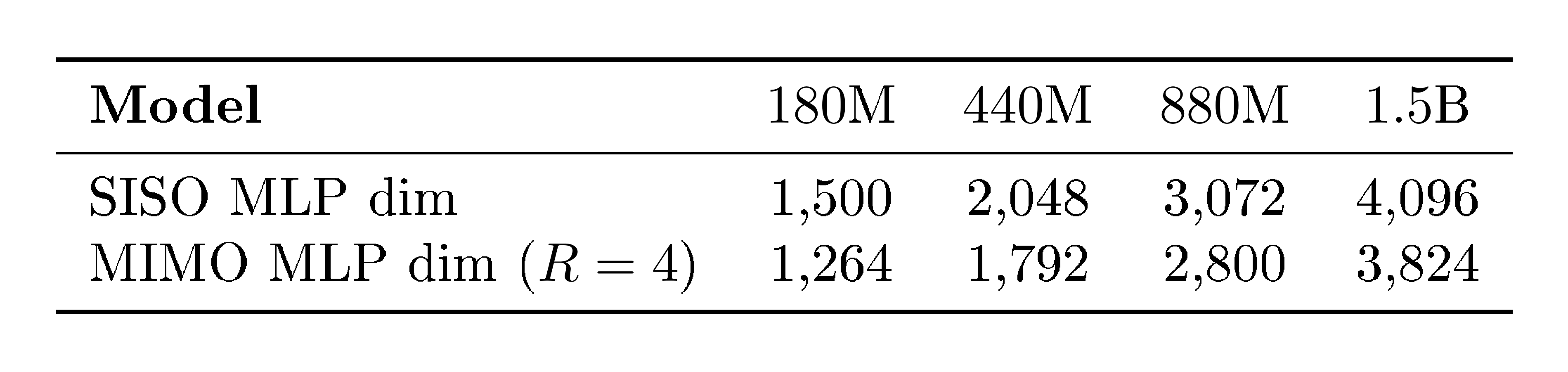
D. Experimental Details

Language Modeling. Our pretraining procedures follow those of [8]'s section D.2. All models at each scale follow the same procedure and were trained with bfloat16. The Mamba family of models were trained using the standard expand factor of $2$ and a $d_\text{state}$ of 128 and head dimension of 64. The Transformer baselines follow [8], and the GDN baselines follow ([30]) where $q, k_\text{dim}=128, v_\text{dim}=256$. We utilize the Llama-3.1 tokenizer ([27]) for all models.

We utilize LM Evaluation Harness ([55]) to test the zero-shot language modeling capabilities of our pretrained model on LAMBADA (OpenAI version) ([56]), HellaSwag ([57]), PIQA ([58]), Arc-Easy/Arc-Challenge ([59]), WinoGrande ([60]), and OpenBookQA ([61]).

Real-World and Synthetic Retrieval. For our real-world retrieval tasks, we evaluate on the common suite consisting of SWDE ([36]), SQuAD ([62]), FDA ([36]), TriviaQA ([63]), NQ ([64]), and DROP ([65]). We utilize the cloze-formatted version of the aforementioned tasks provided by [36, 38], as the original datasets are in a question-answering format, making it challenging for solely pretrained models. All tasks were truncated to match the training context length. The synthetic NIAH tasks ([37]) were also run with LM Evaluation Harness.

State-Tracking Synthetics. Training follows a sequence length curriculum that sets the minimum length to $3$ and progresses the maximum length from $40$ to $160$. Final models are evaluated at $256$ length. Each curriculum runs for $10^{4}$ steps with batch size $256$. We use one-layer models for Parity and three-layer models for Modular-arithmetic tasks. The state size is chosen to be $64$, and we sweep $d_{\text{model}}\in{32, 64}$ and $8$ learning rates logarithmically spaced between $10^{-4}$ and $10^{-2}$, reporting the best validation accuracy.

E. Additional Experimental Results

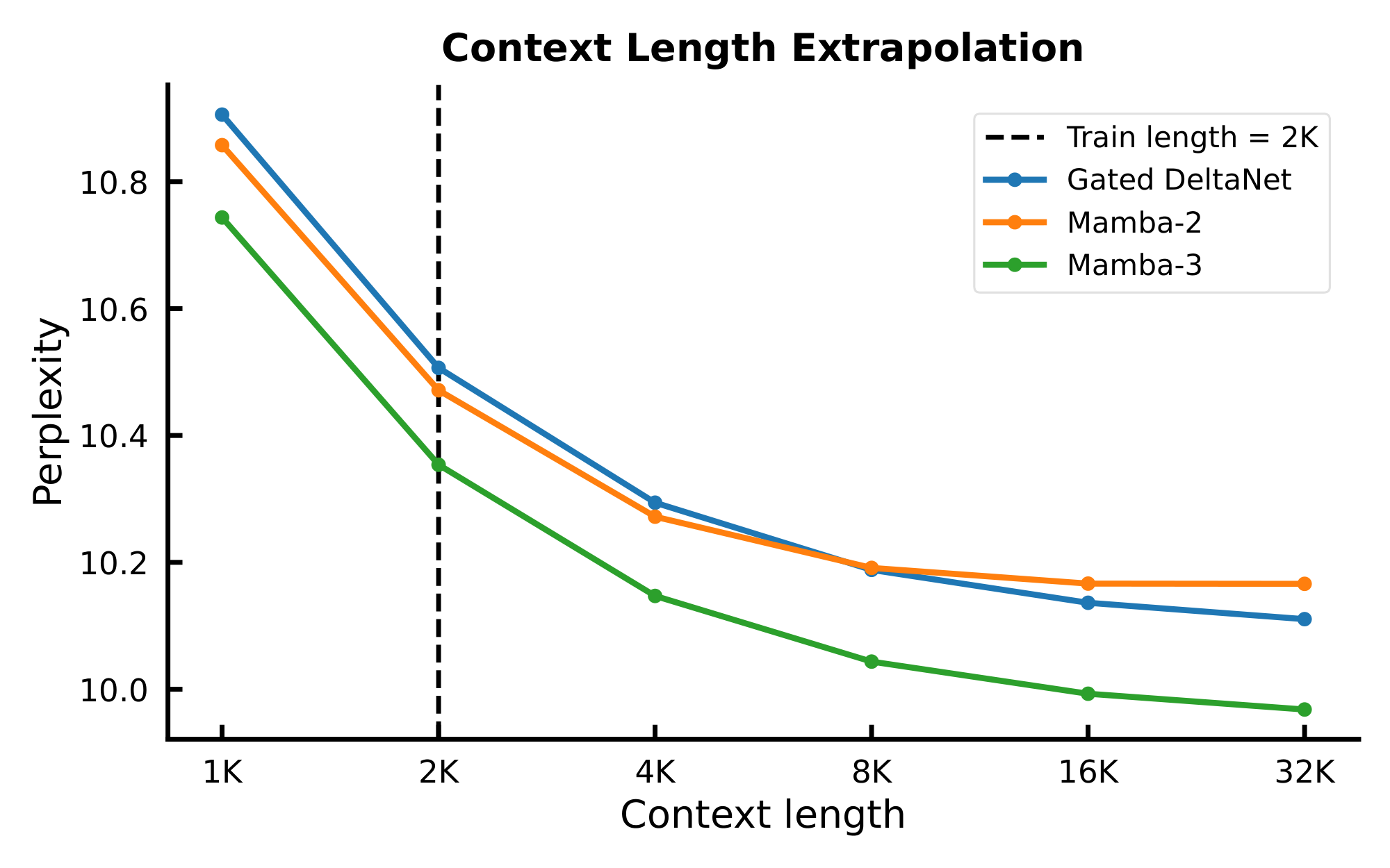
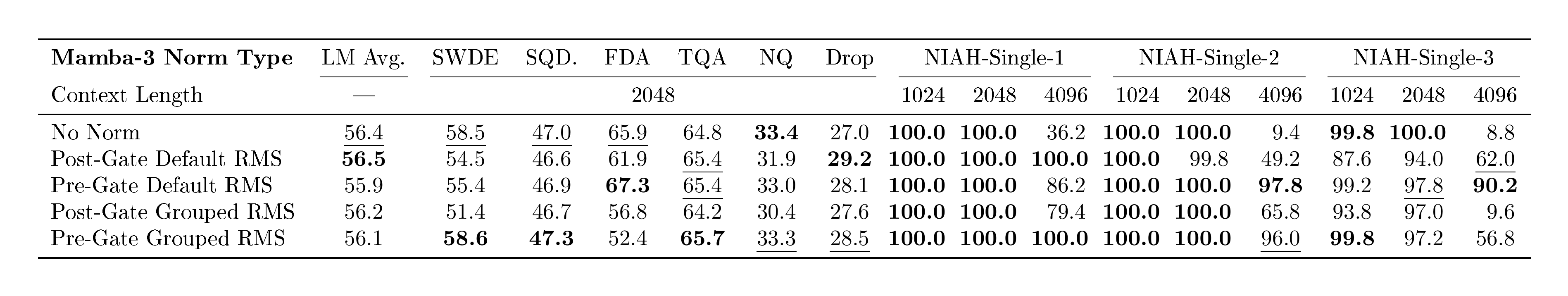
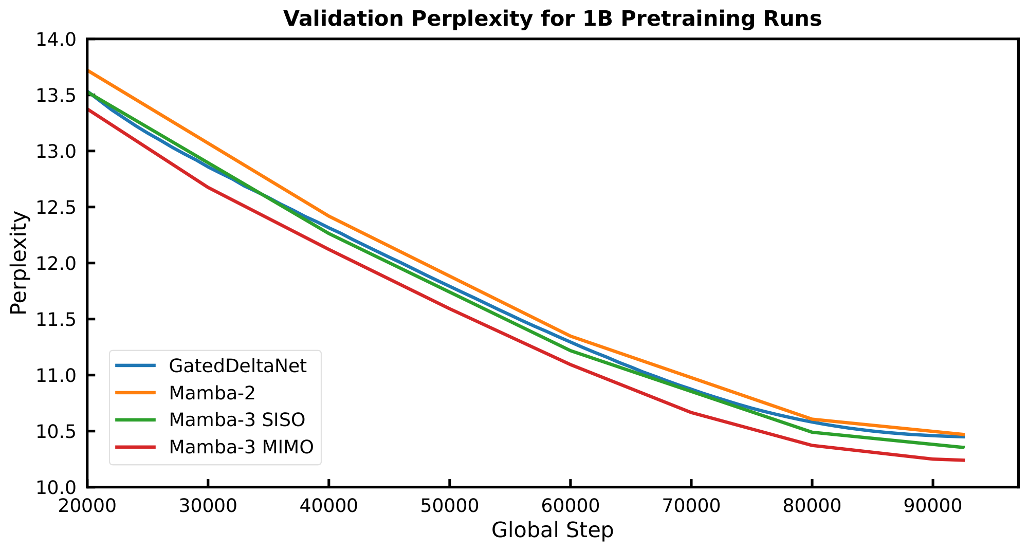
We also compare the effectiveness of state size usage of Mamba variants to a Gated DeltaNet baseline in Figure 7. We highlight the difficulty of directly comparing GDN versus Mamba-style models due to the differing head structure (multi-head for GDN compared to multi-value for Mamba). Our experiments hold GDN's $v_{expand}$ to 2 and decrease the head dimension accordingly to vary the relative total state size. Similar to Figure 3, we train 440M models to $2\times$ Chinchilla tokens ($40\times$ token-to-parameter ratio) and sweep across $d_\text{state}={32, 64, 128}$ for the Mamba models and $d_\text{head dim}={32, 64, 128}$ for GDN. We parameter match all models.

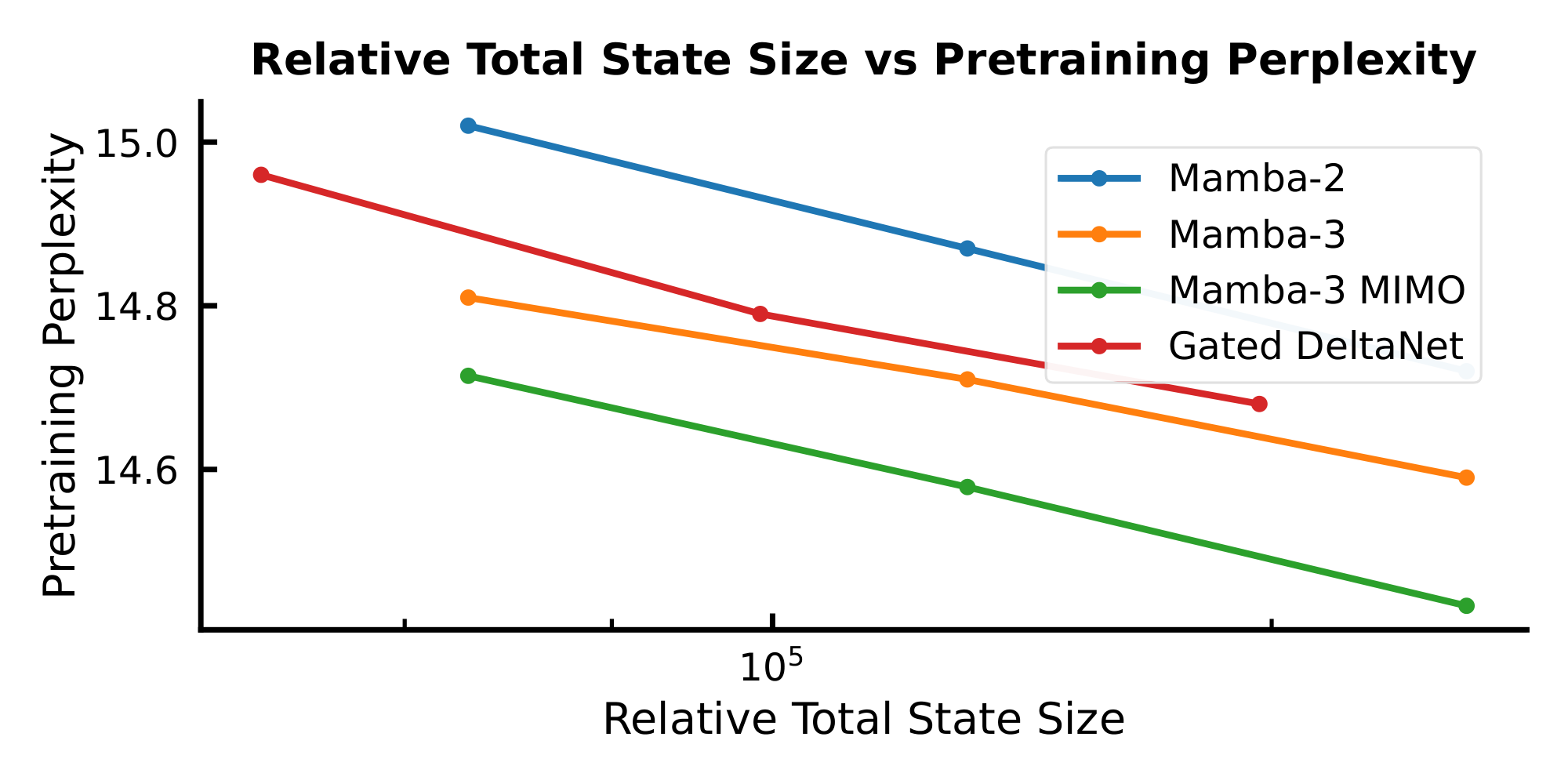
F. Architecture Ablations

We explore our model architecture ablations in this section. All models are trained at the 440M scale to Chinchilla optimal number of tokens ($20\times$ tokens to parameters) with the same experimental procedures as our pretrained models as covered in Appendix D unless otherwise stated.

${\bm{B}}, {\bm{C}}$ Bias Parameterization.

The Mamba-3 model's separate $B$ and $C$ biases are head-specific and channel-wise and added to both ${\bm{B}}$ and ${\bm{C}}$ after the QK-Norm. While the biases in the final Mamba-3 model are trainable, data-independent parameters and initialized to all ones, we explore various bias parameterizations in Table 10. We find our models are not very sensitive to the initialization of the biases as long as they are positive. We choose the all-ones initialization due to its simplicity.

We also explore the impact of removing the $B$ or $C$ bias on performance in Table 10 (bias is initialized with our default parameterization when utilized). Unlike in [32], which finds that $B$ bias by itself is able to improve performance on Mamba-1, our experiments find that only having $B$ bias hurts performance slightly and that $B$ and $C$ biases have synergistic properties.

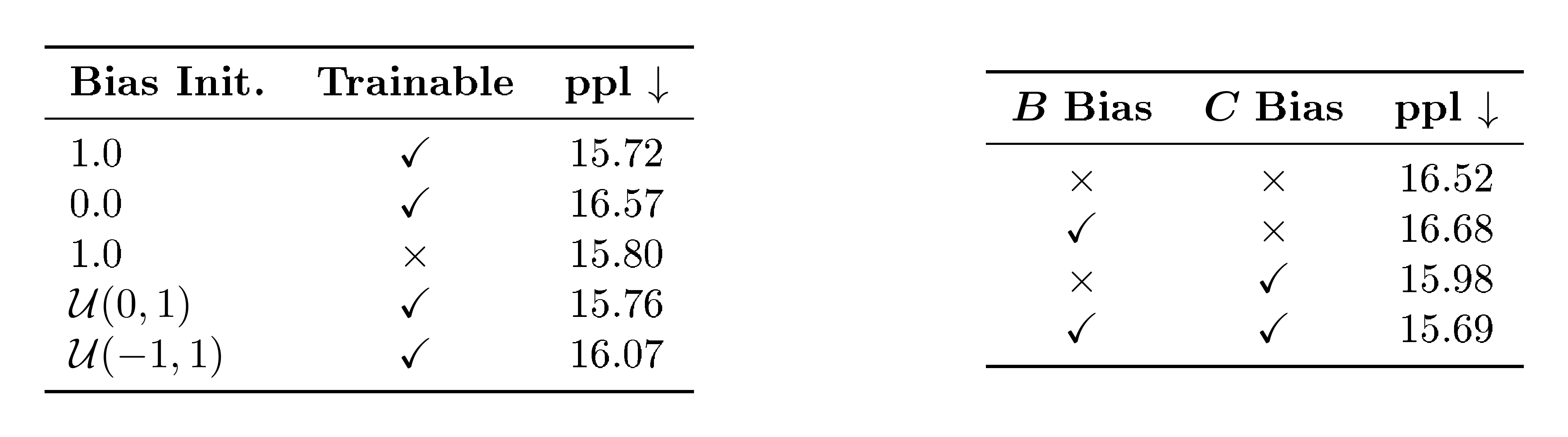
G. Inference Kernel Latency Analysis

G.1 Kernel Implementations and Fusion Structure

In Table 6, we detail the DSL (Triton, TileLang, CuTe, PyTorch) and the fusion level of the kernels used in our latency analysis. For Mamba-2 and Gated DeltaNet (GDN), we directly use the publicly released Triton kernels from the respective authors. For Mamba-3, we implement new inference kernels with a comparable fusion structure: the forward SISO uses a Triton kernel fused with rotary position embeddings and the forward MIMO uses a TileLang kernel with the same fusion level while the decode path uses a CuTe kernel fused with gating and MIMO projection.

In Table 11 and Table 12, we abbreviate IP = input projection, Conv = 1D convolution, Gate = gating, OP = output projection. Colors indicate implementation backend (Torch, Triton, TileLang, CuTe).

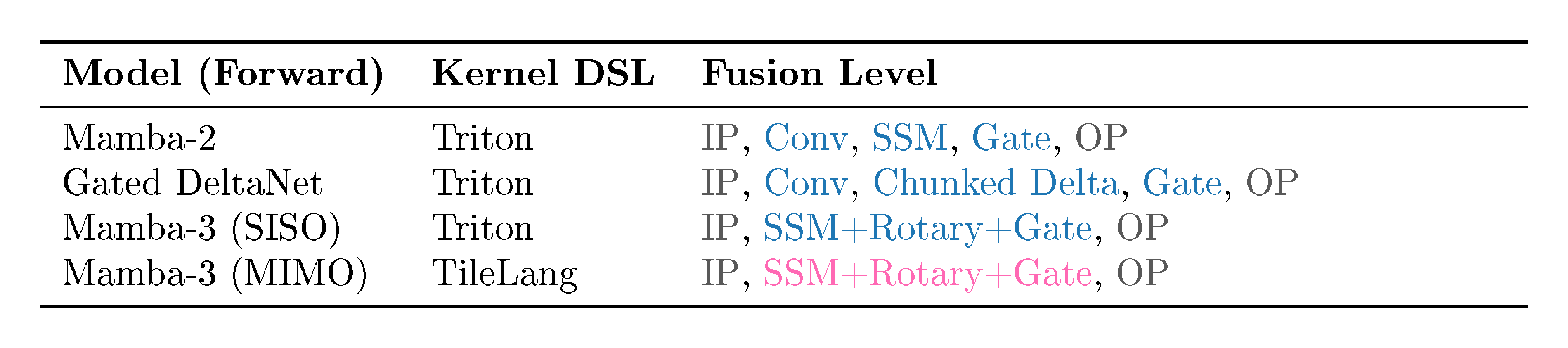
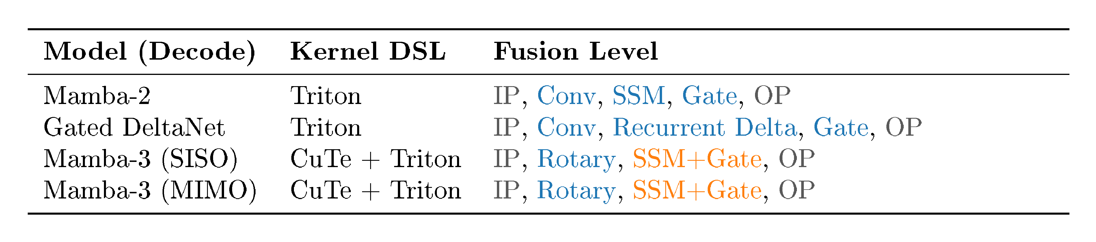
G.2 Extended Prefill and Prefill+Decode Latency Measurements

Models.

We benchmark Mamba-3 1.5B (SISO), Mamba-2 1.5B, Gated DeltaNet 1.5B, and a strong Transformer baseline implemented via the vLLM engine (v0.11.0) with Llama-3.2 1B.^5 All recurrent models are trained at the 1.5B scale with $d_{\text{model}} = 2048$ and $24$ layers. For Mamba variants we set state size as $128$ and head dimension $64$; for GDN we use QK head dimension as $128$.

Setting.

Sequence lengths were swept over $L \in {512, 1024, 2048, 4096, 16384}$ for prefill, with an equal number of tokens decoded. For all sequence lengths, we use a batch size of 128. To report vLLM numbers at sequence length $16384$, we measure performance at the same sequence length with batch size 16. We then scale the result by a factor of 8 to approximate performance at batch size 128 since direct measurement at this setting exceeds GPU memory. This provides a reasonable estimate because each batch is processed independently by each SM on the GPU, so we expect performance of Transformer models to scale linearly with batch size. For recurrent models, when the size of input and output tensors exceeds GPU memory at sequence length $16384$, we utilize a state passing approach that processes the sequence in two halves while propagating the hidden state between segments to avoid materializing the entire sequence at once. We use a single H100-SXM 80GB GPU and report wall-clock times (in seconds) over three repetitions.

We observe that (i) Mamba-3 adds minimal forward-pass cost, showing that the exponential-trapezoidal update, complex state tracking, and MIMO parameterization remain lightweight; (ii) decode latency is competitive across recurrent models; and (iii) recurrent mixers scale more gently with context length than vLLM Llama-3.2-1B, which grows much faster with $L$ due to KV-cache overhead.

References

[1] Yangzhen Wu et al. (2025). Inference Scaling Laws: An Empirical Analysis of Compute-Optimal Inference for Problem-Solving with Language Models. https://arxiv.org/abs/2408.00724.

[2] Charlie Snell et al. (2024). Scaling LLM Test-Time Compute Optimally can be More Effective than Scaling Model Parameters. https://arxiv.org/abs/2408.03314.

[3] OpenAI (2026). Introducing GPT-5.3-Codex. https://openai.com/index/introducing-gpt-5-3-codex/.

[4] Anthropic (2026). Introducing Claude Opus 4.6. https://www.anthropic.com/news/claude-opus-4-6.

[5] Woosuk Kwon et al. (2023). Efficient Memory Management for Large Language Model Serving with PagedAttention. https://arxiv.org/abs/2309.06180.

[6] Baolin Li et al. (2024). LLM Inference Serving: Survey of Recent Advances and Opportunities. https://arxiv.org/abs/2407.12391.

[7] Vaswani et al. (2017). Attention is all you need. In Advances in neural information processing systems. pp. 5998–6008. http://arxiv.org/abs/1706.03762.

[8] Tri Dao and Albert Gu (2024). Transformers are SSMs: Generalized Models and Efficient Algorithms Through Structured State Space Duality. https://arxiv.org/abs/2405.21060.

[9] Imanol Schlag et al. (2021). Linear Transformers Are Secretly Fast Weight Programmers. https://arxiv.org/abs/2102.11174.

[10] Songlin Yang et al. (2025). Parallelizing Linear Transformers with the Delta Rule over Sequence Length. https://arxiv.org/abs/2406.06484.

[11] NVIDIA et al. (2025). Nemotron-H: A Family of Accurate and Efficient Hybrid Mamba-Transformer Models. https://arxiv.org/abs/2504.03624.

[12] An Yang et al. (2025). Qwen3 Technical Report. https://arxiv.org/abs/2505.09388.

[13] Kimi Team et al. (2025). Kimi Linear: An Expressive, Efficient Attention Architecture. https://arxiv.org/abs/2510.26692.

[14] Tencent Hunyuan Team et al. (2025). Hunyuan-TurboS: Advancing Large Language Models through Mamba-Transformer Synergy and Adaptive Chain-of-Thought. https://arxiv.org/abs/2505.15431.

[15] Albert Gu and Tri Dao (2024). Mamba: Linear-Time Sequence Modeling with Selective State Spaces. https://arxiv.org/abs/2312.00752.

[16] Riccardo Grazzi et al. (2025). Unlocking State-Tracking in Linear RNNs Through Negative Eigenvalues. https://arxiv.org/abs/2411.12537.

[17] Yash Sarrof et al. (2024). The Expressive Capacity of State Space Models: A Formal Language Perspective. https://arxiv.org/abs/2405.17394.

[18] Jianlin Su et al. (2023). RoFormer: Enhanced Transformer with Rotary Position Embedding. https://arxiv.org/abs/2104.09864.

[19] Angelos Katharopoulos et al. (2020). Transformers are RNNs: Fast Autoregressive Transformers with Linear Attention. https://arxiv.org/abs/2006.16236.

[20] Albert Gu et al. (2022). Efficiently Modeling Long Sequences with Structured State Spaces. https://arxiv.org/abs/2111.00396.

[21] Gu et al. (2022). On the Parameterization and Initialization of Diagonal State Space Models. arXiv preprint arXiv:2206.11893. https://arxiv.org/abs/2206.11893.

[22] Jimmy T. H. Smith et al. (2023). Simplified State Space Layers for Sequence Modeling. https://arxiv.org/abs/2208.04933.

[23] Süli, Endre and Mayers, David F. (2003). An Introduction to Numerical Analysis. Cambridge University Press.

[24] William Merrill et al. (2025). The Illusion of State in State-Space Models. https://arxiv.org/abs/2404.08819.

[25] Riccardo Grazzi et al. (2024). Is Mamba Capable of In-Context Learning?. https://arxiv.org/abs/2402.03170.

[26] NVIDIA (2022). NVIDIA H100 Tensor Core GPU White Paper. https://resources.nvidia.com/en-us-hopper-architecture/nvidia-h100-tensor-c.

[27] Aaron Grattafiori et al. (2024). The Llama 3 Herd of Models. https://arxiv.org/abs/2407.21783.

[28] Alex Henry et al. (2020). Query-Key Normalization for Transformers. https://arxiv.org/abs/2010.04245.

[29] Mitchell Wortsman et al. (2023). Small-scale proxies for large-scale Transformer training instabilities. https://arxiv.org/abs/2309.14322.

[30] Songlin Yang et al. (2025). Gated Delta Networks: Improving Mamba2 with Delta Rule. https://arxiv.org/abs/2412.06464.

[31] Jiaxi Hu et al. (2025). Comba: Improving Bilinear RNNs with Closed-loop Control. https://arxiv.org/abs/2506.02475.

[32] Annan Yu and N. Benjamin Erichson (2025). Block-Biased Mamba for Long-Range Sequence Processing. https://arxiv.org/abs/2505.09022.

[33] Guilherme Penedo et al. (2024). The FineWeb Datasets: Decanting the Web for the Finest Text Data at Scale. https://arxiv.org/abs/2406.17557.

[34] Allen-Zhu, Zeyuan (2025). Physics of Language Models: Part 4.1, Architecture Design and the Magic of Canon Layers. SSRN Electronic Journal.

[35] Aryaman Arora et al. (2025). Mechanistic evaluation of Transformers and state space models. https://arxiv.org/abs/2505.15105.

[36] Simran Arora et al. (2025). Simple linear attention language models balance the recall-throughput tradeoff. https://arxiv.org/abs/2402.18668.

[37] Cheng-Ping Hsieh et al. (2024). RULER: What's the Real Context Size of Your Long-Context Language Models?. https://arxiv.org/abs/2404.06654.

[38] Simran Arora et al. (2024). Just read twice: closing the recall gap for recurrent language models. https://arxiv.org/abs/2407.05483.

[39] Bowen Yang et al. (2025). Rope to Nope and Back Again: A New Hybrid Attention Strategy. https://arxiv.org/abs/2501.18795.

[40] Roger Waleffe et al. (2024). An Empirical Study of Mamba-based Language Models. https://arxiv.org/abs/2406.07887.

[41] Loïc Cabannes et al. (2025). Short window attention enables long-term memorization. https://arxiv.org/abs/2509.24552.

[42] Dzmitry Bahdanau et al. (2014). Neural Machine Translation by Jointly Learning to Align and Translate. https://arxiv.org/abs/1409.0473.

[43] Krzysztof Choromanski et al. (2022). Rethinking Attention with Performers. https://arxiv.org/abs/2009.14794.

[44] Yutao Sun et al. (2023). Retentive Network: A Successor to Transformer for Large Language Models. https://arxiv.org/abs/2307.08621.

[45] Songlin Yang et al. (2024). Gated Linear Attention Transformers with Hardware-Efficient Training. https://arxiv.org/abs/2312.06635.

[46] Yu Sun et al. (2025). Learning to (Learn at Test Time): RNNs with Expressive Hidden States. https://arxiv.org/abs/2407.04620.

[47] Tianyuan Zhang et al. (2025). Test-Time Training Done Right. https://arxiv.org/abs/2505.23884.

[48] Arnuv Tandon et al. (2025). End-to-End Test-Time Training for Long Context. https://arxiv.org/abs/2512.23675.

[49] Ke Alexander Wang et al. (2025). Test-time regression: a unifying framework for designing sequence models with associative memory. https://arxiv.org/abs/2501.12352.

[50] Ankit Gupta et al. (2022). Diagonal State Spaces are as Effective as Structured State Spaces. https://arxiv.org/abs/2203.14343.

[51] Daniel Y. Fu et al. (2023). Hungry Hungry Hippos: Towards Language Modeling with State Space Models. https://arxiv.org/abs/2212.14052.

[52] Xuezhe Ma et al. (2024). Megalodon: Efficient LLM Pretraining and Inference with Unlimited Context Length. https://arxiv.org/abs/2404.08801.

[53] Antonio Orvieto et al. (2023). Resurrecting Recurrent Neural Networks for Long Sequences. https://arxiv.org/abs/2303.06349.

[54] Tenenbaum, M. and Pollard, H. (1985). Ordinary Differential Equations: An Elementary Textbook for Students of Mathematics, Engineering, and the Sciences. Dover Publications. https://books.google.com/books?id=iU4zDAAAQBAJ.

[55] Gao et al. (2024). The Language Model Evaluation Harness. doi:10.5281/zenodo.12608602. https://zenodo.org/records/12608602.

[56] Denis Paperno et al. (2016). The LAMBADA dataset: Word prediction requiring a broad discourse context. https://arxiv.org/abs/1606.06031.

[57] Rowan Zellers et al. (2019). HellaSwag: Can a Machine Really Finish Your Sentence?. https://arxiv.org/abs/1905.07830.

[58] Yonatan Bisk et al. (2019). PIQA: Reasoning about Physical Commonsense in Natural Language. https://arxiv.org/abs/1911.11641.

[59] Peter Clark et al. (2018). Think you have Solved Question Answering? Try ARC, the AI2 Reasoning Challenge. https://arxiv.org/abs/1803.05457.

[60] Keisuke Sakaguchi et al. (2019). WinoGrande: An Adversarial Winograd Schema Challenge at Scale. https://arxiv.org/abs/1907.10641.

[61] Todor Mihaylov et al. (2018). Can a Suit of Armor Conduct Electricity? A New Dataset for Open Book Question Answering. https://arxiv.org/abs/1809.02789.

[62] Pranav Rajpurkar et al. (2018). Know What You Don't Know: Unanswerable Questions for SQuAD. In ACL 2018.

[63] Mandar Joshi et al. (2017). TriviaQA: A Large Scale Distantly Supervised Challenge Dataset for Reading Comprehension. https://arxiv.org/abs/1705.03551.

[64] Kwiatkowski et al. (2019). Natural Questions: A Benchmark for Question Answering Research. Transactions of the Association for Computational Linguistics. 7. pp. 452–466. doi:10.1162/tacl_a_00276. https://aclanthology.org/Q19-1026/.

[65] Dheeru Dua et al. (2019). DROP: A Reading Comprehension Benchmark Requiring Discrete Reasoning Over Paragraphs. https://arxiv.org/abs/1903.00161.