Reasoning with Sampling: Your Base Model is Smarter Than You Think

Aayush Karan$^1$, Yilun Du$^1$

$^1$Harvard University

🌐 Website GitHub Code

Abstract

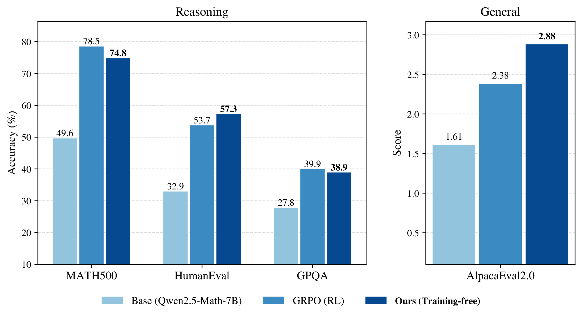
Frontier reasoning models have exhibited incredible capabilities across a wide array of disciplines, driven by posttraining large language models (LLMs) with reinforcement learning (RL). However, despite the widespread success of this paradigm, much of the literature has been devoted to disentangling truly novel behaviors that emerge during RL but are not present in the base models. In our work, we approach this question from a different angle, instead asking whether comparable reasoning capabilites can be elicited from base models at inference time by pure sampling, without any additional training. Inspired by Markov chain Monte Carlo (MCMC) techniques for sampling from sharpened distributions, we propose a simple iterative sampling algorithm leveraging the base models' own likelihoods. Over different base models, we show that our algorithm offers substantial boosts in reasoning that nearly match and even outperform those from RL on a wide variety of single-shot tasks, including MATH500, HumanEval, and GPQA. Moreover, our sampler avoids the collapse in diversity over multiple samples that is characteristic of RL-posttraining. Crucially, our method does not require training, curated datasets, or a verifier, suggesting broad applicability beyond easily verifiable domains.

Executive Summary: Large language models (LLMs) have transformed fields like mathematics, coding, and science by generating reasoned responses, often enhanced through reinforcement learning (RL), a training process that refines models using rewards. However, RL requires vast computational resources, curated datasets, and reliable verifiers, raising questions about whether it truly unlocks new abilities or merely sharpens what base models—pre-trained LLMs without this extra step—already possess. This matters now as organizations seek cost-effective ways to deploy capable AI, especially amid rising energy and data demands, without the risks of RL, such as reduced output variety.

This document sets out to test whether base LLMs can produce single-response reasoning on par with RL-enhanced versions using only inference-time adjustments—no training involved. It proposes and evaluates a simple sampling technique to draw higher-quality outputs from base models.

The authors developed a sampling algorithm inspired by statistical methods for exploring probability distributions. They applied it to three base LLMs (Qwen2.5-Math-7B for math, Qwen2.5-7B for general tasks, and Phi-3.5-mini-instruct for coding) across four benchmarks spanning 2023–2024 datasets: MATH500 (500 math problems), HumanEval (164 coding tasks), GPQA (198 science questions), and AlpacaEval 2.0 (805 general queries). The method iteratively refines generated text by resampling segments based on the base model's own probability estimates, using a "power distribution" concept to favor high-likelihood paths. Experiments compared this to RL baselines (like Group Relative Policy Optimization) over thousands of trials, assuming the base model's probabilities reliably signal good reasoning without external rewards.

Key findings show the sampling method dramatically improves base model performance. First, it boosts single-response accuracy by 25–52 percentage points across tasks—for instance, raising MATH500 solve rates from 20–30% to 45–55%, nearly matching RL gains. Second, it outperforms RL on unfamiliar tasks, such as improving HumanEval coding success by up to 60% more than RL versions, and yielding 10–15% higher win rates on general queries in AlpacaEval. Third, unlike RL, which narrows output variety (hurting multi-sample performance beyond the first try), this approach sustains diversity, achieving 20–40% better success rates when generating 2–64 samples per query. Fourth, it naturally produces longer, more detailed responses (about 10–15% longer) without explicit instructions. Finally, the compute cost equates to roughly one RL training cycle per task, using 8–9 times more tokens than standard generation but far less than full RL.

These results imply that base LLMs harbor untapped reasoning potential, often masked by basic sampling; RL may just redistribute existing strengths rather than invent new ones. This shifts impacts toward lower costs (no dataset curation or retraining), better reliability (preserved variety reduces risks in applications like code debugging or scientific analysis), and wider access (works without verifiers for non-testable domains). Contrary to prior views that RL introduces novel behaviors, these findings suggest sharpening base distributions via sampling can rival or exceed RL, especially outside trained areas, potentially accelerating AI deployment timelines by months.

Leaders should integrate this sampling into inference pipelines for reasoning-heavy uses, starting with math and coding tools to gain RL-like boosts without retraining. For broader adoption, test it on proprietary models and tasks, weighing trade-offs like 8–10x inference slowdown against performance gains. If scaling to larger LLMs, invest in hardware for the extra compute. Further steps include piloting on real workflows (e.g., enterprise coding) and analyzing more diverse benchmarks to confirm generalizability; additional tuning of parameters like resampling steps could optimize for speed.

While robust on the tested 7-billion-parameter models and verifiable tasks, limitations include reliance on strong base LLMs (weaker ones may see smaller gains) and higher compute for long outputs, plus untested edge cases like multilingual or creative reasoning. Confidence is high for math, coding, and science domains based on consistent benchmarks, but readers should validate cautiously in unexamined areas before full rollout.

1. Introduction

Section Summary: Reinforcement learning has become a key method for improving the reasoning skills of large language models, but experts question whether it creates truly new abilities or simply sharpens the model's existing tendencies toward more confident outputs. This paper shows that a clever sampling technique applied directly to untrained base models can match or even surpass the single-shot reasoning performance of RL-trained models on familiar tasks and outperform them on unfamiliar ones, all while maintaining the model's output diversity. The approach requires no extra training, datasets, or verification tools, and it demonstrates that base models are already capable of strong reasoning when sampled effectively.

Reinforcement learning (RL) has become the dominant paradigm for enhancing the reasoning capabilities of large language models (LLMs) ([1, 2]). Equipped with a reward signal that is typically automatically verifiable, popular RL techniques have been successfully applied to posttrain frontier models, leading to sizeable performance gains in domains like math, coding, and science ([3, 4, 5]).

Despite the widespread empirical success of RL for LLMs, a large body of literature has centered around the following question: are the capabilities that emerge during RL-posttraining fundamentally novel behaviors that are not present in the base models? This is the question of distribution sharpening ([6, 7, 8]): that is, whether the posttrained distribution is simply a "sharper" version of the base model distribution, instead of placing mass on reasoning traces the base model is unlikely to generate.

Several works point towards the difficulty in learning new capabilities with RL-posttraining. [6, 9] compare the pass@ $k$ (multi-shot) scores of base models with posttrained models, finding that for large $k$, base models actually outperform while the latter suffer from degraded generation diversity. In such cases, RL appears to redistribute pass@ $k$ performance to single-shot performance at the expense of multi-shot reasoning. [8] also notes that the reasoning traces post-RL are tightly concentrated at high likelihoods/confidences under the base model, seemingly drawing from existing high-likelihood capabilities. We illustrate this point in our own experiments in Figure 4. Regardless, the advantage of RL-posttraining for single-shot reasoning has remained, as of yet, undeniable.

In this paper, we present a surprising result: sampling directly from the base model can achieve single-shot reasoning capabilites on par with those from RL.

We propose a sampling algorithm for base models that leverages additional compute at inference time, achieving single-shot performance that nearly matches RL-posttraining on in-domain reasoning tasks and can even outperform on out-of-domain reasoning tasks. Furthermore, we observe that generation diversity does not degrade with our sampler; in fact, our pass@ $k$ (multi-shot) performance strongly outperforms RL. We benchmark specifically against Group Relative Policy Optimization (GRPO), which is the standard RL algorithm for enhancing LLM reasoning ([10]).

Crucially, our algorithm is training-free, dataset-free, and verifier-free, avoiding some of the inherent weaknesses of RL methods including extensive hyperparameter sweeps to avoid training instabilities, the need to curate a diverse and expansive posttraining dataset, and the lack of guaranteed access to a ground truth verifier/reward signal ([11]).

Our contributions can be summarized as follows:

• i) We introduce the power distribution as a useful sampling target for reasoning tasks. Since it can be explicitly specified with a base LLM, no additional training is required.
• ii) We further introduce an approximate sampling algorithm for the power distribution using a Markov chain Monte Carlo (MCMC) algorithm that iteratively resamples token subsequences according to their base model likelihoods.
• iii) We empirically demonstrate the effectiveness of our algorithm over a range of models (Qwen2.5-Math-7B, Qwen2.5-7B, Phi-3.5-mini-instruct) and reasoning tasks (MATH500, HumanEval, GPQA, AlpacaEval 2.0). Our results show that sampling directly from the base model can achieve results on par with GRPO. In fact, for some out-of-domain tasks, our algorithm consistently outperforms the RL baseline. Moreover, over multiple samples, we avoid the collapse in diversity afflicting RL-posttraining, achieving the best of both worlds in terms of single-to-few-shot reasoning capabilities as well as sample diversity.

Our results collectively illustrate that existing base models are much more capable at single-shot reasoning than current sampling methods reveal.

2. Related Works

Section Summary: Researchers have used reinforcement learning techniques, such as RLHF and the newer RLVR, to fine-tune large language models after initial training, helping them align better with human preferences and excel at challenging tasks like math and coding, often without needing extra training in some innovative approaches. Related studies have adapted classic sampling methods like MCMC for language models to generate text that targets specific reward-based distributions, similar to techniques in sequential Monte Carlo or Metropolis-Hastings algorithms, though the current work avoids external rewards entirely. In the field of diffusion models, annealed or tempered sampling draws from statistical physics to prevent issues like mode collapse, enabling more accurate sampling from complex distributions and improving outputs in areas like protein design.

Reinforcement learning for LLMs.

RL has been instrumental in posttraining LLMs. Early on, RL with human feedback (RLHF) ([12]) was developed as a technique to align LLMs with human preferences using a trained reward model. Recently, RL with verifiable rewards (RLVR) has emerged as a powerful new posttraining technique, where many works ([1, 13, 2, 14]) discovered that a simple, end-of-generation reward given by an automated verifier could substantially enhance performance on difficult reasoning tasks in mathematics and coding. The Group Relative Policy Optimization (GRPO) algorithm was at the center of these advances ([10]). Building off of this success, many subsequent works have examined using reward signals derived from internal signals such as self-entropy ([15]), confidence ([11]), and even random rewards ([7]). Similar to these works, our paper examines base model likelihoods as a mechanism for improving reasoning performance, but crucially, our technique is training-free.

Autoregressive MCMC sampling with LLMs.

Prior works have explored integrating classic MCMC techniques with autoregressive sampling. Many settings including red-teaming, prompt-engineering, and personalized generation can be framed as targeting sampling from the base LLM distribution but tilted towards an external reward function. [16] proposes learning intermediate value functions that are used in a Sequential Monte Carlo (SMC) framework ([17]), where multiple candidate sequences are maintained and updated according to their expected future reward. Similarly, [18] proposes a Metropolis-Hastings (MH) algorithm, which instead of maintaining multiple candidates performs iterative resampling, again updating according to expected reward. Methodologically, our sampling algorithm is most similar to this latter work, but the crucial difference is that our target sampling distribution is completely specified by the base LLM, avoiding the need for an external reward.

Annealed sampling for diffusion.

In the statistical physics and Monte Carlo literature, sampling from $p^{\alpha}$ is known as sampling from an annealed, or tempered, distribution ([19]) and has inspired a new wave of interest within the diffusion community. Indeed, in traditional MCMC sampling, annealing is used as a way to avoid mode-collapse during sampling and more accurately sample from complex multimodal distributions ([20]). This has re-emerged as inference-time sampling methods for diffusion that aim to steer a pretrained model towards "tilted distributions" ([21, 22, 23, 24, 25, 26]). Where traditional RL techniques exhibit mode collapse, applications in the physical sciences ([27]) require multimodal sampling. To this end, works such as [21, 24, 22] construct sequences of annealed distributions to ease the transition from base diffusion distribution to tilted distribution. Other works ([28, 29]) intentionally target sampling from $p^{\alpha}$ for $\alpha > 1$ as a means of generating higher quality samples from the base diffusion model, which is particularly popular for generating more designable proteins ([30]).

3. Preliminaries

Section Summary: This section introduces the basic setup for language models, starting with a fixed set of tokens like words or word parts that make up text. It explains how a large language model generates sequences of these tokens by predicting each new one based only on the previous ones, which combines to form the full probability of the entire sequence. To create new text, the model samples tokens one by one using these predictions, ensuring the result follows the model's learned distribution.

Let $\mathcal{X}$ be a finite vocabulary of tokens, and let $\mathcal{X}^T$ denote the set of finite sequences of tokens $x_{0:T} = (x_0, x_1, \dots, x_T)$, where $x_i \in \mathcal{X}$ for all $i$ and $T \in \mathbb{Z}{\geq 0}$ is some nonnegative integer. For convenience, for a given $t$, let $x{<t} = (x_0, \dots, x_{t-1})$ and $x_{>t} = (x_{t+1}, \dots, x_{T})$, with similar definitions for $x_{\leq t}$ and $x_{\geq t}$. In general, $\mathbf{x}$ refers to a token sequence $x_{0:T}$, where $T$ is implicitly given.

Then an LLM defines a distribution $p$ over token sequences $\mathcal{X}^T$ by autoregressively learning the conditional token distributions $p(x_t | x_{<t})$ for all $t$, giving the joint distribution via the identity

$ p(x_{0:T}) = \prod_{t=0}^T p(x_t | x_{<t}).\tag{1} $

To sample a sequence from $p$, we simply sample from the LLM token by token using the conditional distributions, which by Equation (1) directly samples from the joint distribution.

4. MCMC Sampling for Power Distributions

Section Summary: This section describes a sampling method for language models that sharpens probability distributions to favor high-likelihood outcomes, mimicking the improvements seen in models trained with reinforcement learning. It focuses on power distributions, where raising the original probabilities to a power greater than one boosts the weight of promising sequences while downplaying unlikely ones, which helps generate more reasoned responses. Unlike common low-temperature sampling, which averages future possibilities before sharpening, power distributions sharpen each potential future path individually, leading to preferences for tokens with a few strong continuations over many weaker ones, as shown in a simple example.

In this section, we introduce our sampling algorithm for base models. Our core intuition is derived from the notion of distribution sharpening posed in Section 1. Sharpening a reference distribution refers to reweighting the distribution so that high likelihood regions are further upweighted while low likelihood regions are downweighted, biasing samples heavily towards higher likelihoods under the reference. Then if RL posttrained models really are just sharpened versions of the base model, we should be able to explicitly specify a target sampling distribution that achieves the same effect.

We organize this section as follows. Section 4.1 presents this target sharpened distribution and provides some mathematical motivation for why its samples are amenable for reasoning tasks. Section 4.2 introduces a general class of Markov chain Monte Carlo (MCMC) algorithms aimed at actually sampling from this target distribution, and finally, Section 4.3 details our specific implementation for LLMs.

4.1 Reasoning with Power Distributions

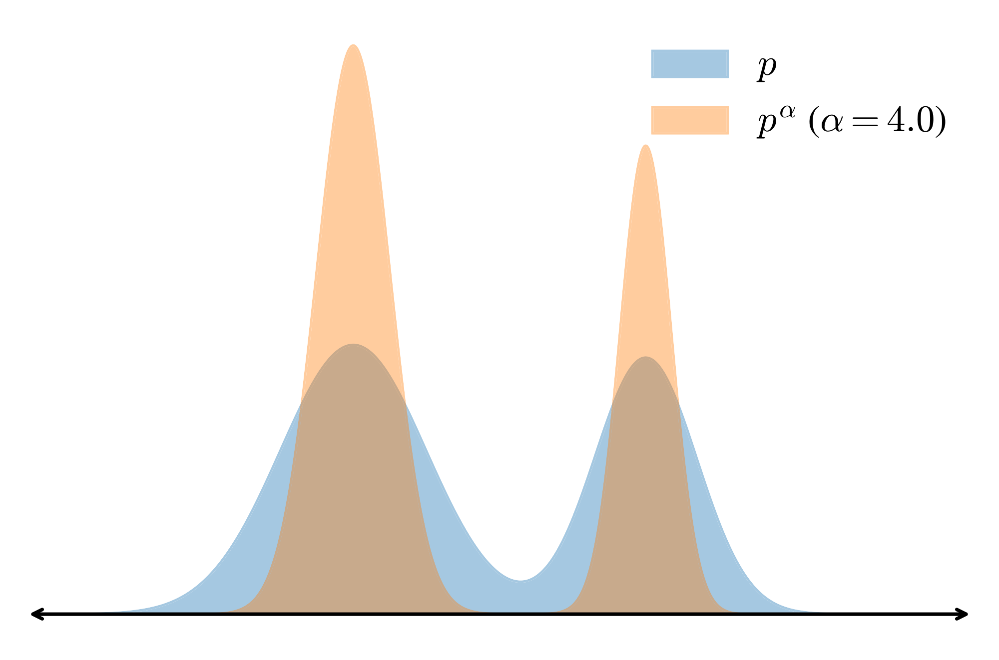
One natural way to sharpen a distribution $p$ is to sample from the power distribution $p^{\alpha}$. Since

$ p(\mathbf{x}) > p(\mathbf{x'}) \implies \frac{p(\mathbf{x})^{\alpha}}{p(\mathbf{x'})^{\alpha}} > \frac{p(\mathbf{x})}{p(\mathbf{x'})} \qquad (\alpha \in [1, \infty]), $

it follows that exponentiating $p$ increases the relative weight on higher likelihood sequences ($\mathbf{x}$) while decreasing the relative weight on lower likelihood ones ($\mathbf{x'}$) (see Figure 2 for a visualization).

A related but well-known sharpening strategy is low-temperature sampling ([31]), which exponentiates the conditional next-token distributions at each step:

$ p_{\text{temp}}(x_t | x_0 \dots x_{t-1}) = \frac{p(x_t | x_{t-1}\dots x_0)^{\alpha}}{\sum_{x_t' \in \mathcal{X}} p(x_t' | x_{t-1}\dots x_0)^{\alpha}},\tag{2} $

where the temperature is $\tau = 1/\alpha$. A common misconception is that sampling with Equation (2) over $T$ tokens is equivalent to sampling from $p^{\alpha}$; however, this is false in a subtle yet crucial way, as we illuminate in the following.

Proposition

Low-temperature sampling does not sample from the power distribution $p^{\alpha}$.

Proof: We show that the associated conditional next-token distributions are distinct at each timestep $t$. The conditional distribution on $x_t$ for $p^{\alpha}$ is given by

$ p_{\text{pow}}(x_t | x_0 \dots x_{t-1}) = \frac{\sum_{x_{>t}} p(x_0, \dots, x_t, \dots, x_T)^{\alpha}}{\sum_{x_{\geq t}} p(x_0, \dots, x_t, \dots, x_T)^{\alpha}}. $

Using Bayes rule

$ p(x_t | x_{t-1} \dots x_0) = \frac{p(x_0, \dots, x_{t})}{p(x_0, \dots, x_{t-1})} = \frac{\sum_{x_{>t}} p(x_0, \dots, x_t, \dots, x_T)}{\sum_{x_{\geq t}} p(x_0, \dots, x_t, \dots, x_T)}, $

we can rewrite the low-temperature marginal Equation (2) as

$ p_{\text{temp}}(x_t | x_0 \dots x_{t-1}) = \frac{\left(\sum_{x_{>t}} p(x_0, \dots, x_t, \dots, x_T)\right)^{\alpha}}{\sum_{x_t'}\left(\sum_{x_{>t}} p(x_0, \dots, x_t, \dots, x_T)\right)^{\alpha}}. $

Ignoring normalizations for clarity, the relative weight on token $x_t$ for sampling from $p^{\alpha}$ is given by a sum of exponents

$ p_{\text{pow}}(x_t | x_{<t}) \propto \sum_{x_{>t}} p(x_0, \dots, x_t, \dots, x_T)^{\alpha}.\tag{3} $

Meanwhile, the relative weight for low-temperature sampling is given by an exponent of sums

$ p_{\text{temp}}(x_t | x_{<t}) \propto \left(\sum_{x_{>t}} p(x_0, \dots, x_t, \dots, x_T)\right)^{\alpha}.\tag{4} $

Since the relative weights of next-token prediction are distinct for each sampling strategy, it follows that the joint distribution over seqeunces must also be distinct for each sampler. Hence, the distribution on sequences given by low-temperature sampling is not the same as the one given by $p^{\alpha}$.

One intuitive way to understand this difference is that low-temperature sampling does not account for how exponentiation sharpens the likelihoods of "future paths" at time step $t$, instead "greedily" averaging all these future likelihoods (exponent of sums Equation (4)). On the other hand, sampling from $p^{\alpha}$ inherently accounts for future completions as it exponentiates all future paths (sum of exponents Equation (3)) before computing the weights for next-token prediction. This has the following consequence:

Observation

The power distribution upweights tokens with few but high likelihood future paths, while low-temperature sampling upweights tokens with several but low likelihood completions.

Example

We can observe this phenomenon with a simple example. Let us consider the token vocabulary $\mathcal{X} = {a, b}$ and restrict our attention to two-token sequences $(x_0, x_1)$: $aa, ab, ba, bb$. Let

$ p(aa) = 0.00, \qquad p(ab) = 0.40, \qquad p(ba) = 0.25, \qquad p(bb) = 0.25, $

so that

$ p(x_0 = a) = 0.40, \qquad p(x_0 = b) = 0.50. \qquad $

Let $\alpha = 2.0$. Under $p^{\alpha}$, we have

$ p_{\text{pow}}(x_0 = a) \propto 0.00^2 + 0.40^2 = 0.160, \qquad p_{\text{pow}}(x_0 = b) \propto 0.25^2 + 0.25^2 = 0.125, $

so $p^{\alpha}$ prefers sampling $a$ over $b$. Under low-temperature sampling,

$ p_{\text{temp}}(x_0 = a) \propto (0.00 + 0.40)^2 = 0.160, \qquad p_{\text{temp}}(x_0 = b) \propto (0.25 + 0.25)^2 = 0.250, $

preferring sampling $b$ over $a$. If $p^{\alpha}$ samples $x_0=a$, there is only one future path with likelihood $0.40$. If $p_{\text{temp}}$ samples $x_0=b$, there are two future paths $ba, bb$, but either choice has likelihood $0.25$.

In other words, even though $a$ has lower conditional likelihood under both $p$ and $p_{\text{temp}}$, $p^{\alpha}$ upweights $a$ and samples the highest likelihood two-token sequence. $b$ has many future paths contributing to a higher likelihood under $p$ and $p_{\text{temp}}$, but leads to low likelihood sequences. We provide a stronger formalization of this phenomenon in Appendix A.1.

Thus, sampling from $p^{\alpha}$ encourages sampling tokens which have fewer but higher likelihood "future paths", as opposed to tokens with several lower likelihood completions. This type of behavior is immensely valuable for reasoning tasks. For example, choosing "wrong" tokens that have high average likelihoods but trap outputs in low likelihood individual futures are examples of critical windows or pivotal tokens ([32, 33]), a phenomenon where a few tokens are highly influential in the correctness of language model outputs. In fact, sharp critical windows have been shown to correlate strongly with reasoning failures ([32]). Instead, embedded in sampling from the power distribution is an implicit bias towards planning for future high likelihood tokens.

4.2 The Metropolis-Hastings

Algorithm

Now that we have seen how sampling from $p^{\alpha}$ can in theory assist the underlying LLM's ability to reason, our aim now turns towards proposing an algorithm to accurately sample from it. Given an LLM $p$, we have access to the values $p^{\alpha}$ over any sequence length; however, these values are unnormalized. Direct sampling from the true probabilities requires normalizing over all sequences $(x_0, \dots, x_T) \in \mathcal{X}^T$, which is computationally intractable.

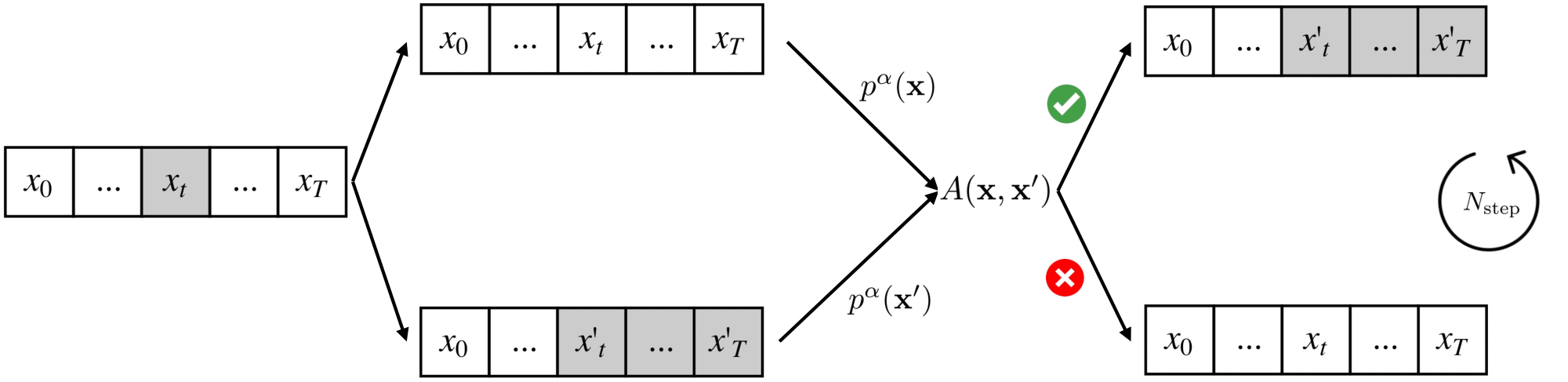
To get around this, we invoke a Markov Chain Monte Carlo (MCMC) algorithm known as Metropolis-Hastings (MH) ([34]), which targets exactly what we want: approximate sampling from an unnormalized probability distribution. The MH algorithm constructs a Markov chain of sample sequences $(\mathbf{x}^0, \mathbf{x}^1, \dots, \mathbf{x}^n)$ using an arbitrary proposal distribution $q(\mathbf{x}|\mathbf{x}^i)$ to select the next candidate $\mathbf{x}^{i+1}$. With probability

$ A(\mathbf{x}, \mathbf{x}^i) = \text{min} \left\lbrace 1, \frac{p^{\alpha}(\mathbf{x}) \cdot q(\mathbf{x}^i | \mathbf{x})}{p^{\alpha}(\mathbf{x}^i) \cdot q(\mathbf{x}|\mathbf{x}^i)}\right\rbrace,\tag{5} $

candidate $\mathbf{x}$ is accepted as $\mathbf{x}^{i+1}$; otherwise, MH sets $\mathbf{x}^{i+1} = \mathbf{x}^{i}$. This algorithm is especially convenient as it only requires the relative weights given by $p^{\alpha}$ (as the normalization weights in $A$ cancel) and works with any generic but tractable sampler $q$ with minimal restrictions. Remarkably, for large enough $n$, this process converges to sampling from the target distribution $p^{\alpha}$ under the following (quite minimal) conditions on the proposal distribution ([35]):

########## caption="\rm The proposal distribution $q$ is irreducible if for any set $X$ with nonzero mass under the target distribution $p^{\alpha}$, $q$ has nonzero probability of eventually sampling from $X$. The proposal is aperiodic if the induced chain of samples does not return to the same sample after a fixed interval number of steps." type="Definition"

Thus, we must simply ensure that our proposal distribution satisfies irreducibility and aperiodicity, and Metropolis-Hastings takes care of the rest. On a practical level, we would also like both $q(\mathbf{x} | \mathbf{x}^i)$ and its reverse $q(\mathbf{x}^i | \mathbf{x})$ to be easily computable.

Consider the following family of random resampling proposal distributions (see Figure 3). Let $p_{\text{prop}}$ be a proposal LLM. With uniform probability $\frac{1}{T}$, select a random $t \in [1, T]$ and resample the sequence starting at index $t$ using $p_{\text{prop}}$. Then the transition likelihood $q(\mathbf{x} | \mathbf{x}^i)$ is simply the likelihood of the resampling. Note that at each candidate selection step, we have a nonzero probability of transitioning between any two sequences $\mathbf{x}, \mathbf{x'} \in \mathcal{X}$, since with some probability we can always resample as early as the beginning of $\mathbf{x}$. This ensures our proposal distribution is both irreducible and aperiodic. Moreover, $q(\mathbf{x}^i | \mathbf{x})$ is easy to calculate by symmetry, since we can treat $\mathbf{x}^i$ as a resampled version of $\mathbf{x}$.

With the flexibility endowed by Metropolis-Hastings, we can choose the proposal LLM $p_{\text{prop}}$ to be any LLM with any sampling strategy (e.g., low-temperature sampling).

4.3 Power Sampling with Autoregressive MCMC

A direct implementation of Metropolis-Hastings for LLMs would involve initializing with a sampled token sequence of length $T$, subsequently generating new candidates of length $T$ with Equation (5) over many, many iterations. This process is computationally expensive, however, due to the repeated, full sequence inference calls to the LLM.

In fact, the main downside to MCMC algorithms in practice is the potential for an exponential mixing time ([36]), where a poor choice of initialization or proposal distribution can result in an exponentially large number of samples required before convergence to the target distribution. This problem is exacerbated if the sample space has high dimensionality ([37, 38]), which is precisely exhibited by the sequence space of tokens $\mathcal{X}^T$, especially for long sequences/large values of $T$.

To remedy this, we propose an algorithm that leverages the sequential structure of autoregressive sampling. We define a series of intermediate distributions which we progressively sample from, until converging to the target distribution $p^{\alpha}$. In particular, samples from one intermediate distribution initiate a Metropolis-Hastings process for the next, helping avoid pathological initializations.

Fix block size $B$ and proposal LLM $p_{\text{prop}}$, and consider the sequence of (unnormalized) distributions

$ \emptyset \longrightarrow p(x_0, \dots, x_B)^{\alpha} \longrightarrow p(x_0, \dots, x_{2B})^{\alpha} \longrightarrow \dots \longrightarrow p(x_0, \dots, x_T)^{\alpha}, $

where $p(x_0, \dots, x_{kB})$ denotes the joint distribution over token sequences of length $kB$, for any $k$. For convenience, let $\pi_k$ denote the distribution given by

$ \pi_k(x_{0:kB}) \propto p(x_{0:kB})^{\alpha}. $

Suppose we have a sample from $\pi_k$. To obtain a sample from $\pi_{k+1}$, we initialize a Metropolis-Hastings process by sampling the next $B$ tokens $x_{kB+1:(k+1)B}$ with $p_{\text{prop}}$. We subsequently run the MCMC sampling procedure for $N_{\text{MCMC}}$ steps, using the random resampling proposal distribution $q$ from the previous section. The full details are presented in Algorithm 1.

**Input:** base $p$; proposal $p_{\mathrm{prop}}$; power $\alpha$; length $T$
**Hyperparams:** block size $B$; MCMC steps $N_{\mathrm{MCMC}}$
**Output:** $(x_0,\dots,x_T) \sim p^\alpha$
**Notation:** Define the unnormalized intermediate target
$
{\pi}_k(x_{0:kB}) \propto p(x_{0:kB})^{\alpha}.
$
**for** $k \gets 0$ to $\lceil \frac{T}B\rceil-1$:
    Given prefix $x_{0:kB}$, we wish to sample from $\pi_{k+1}$. Construct initialization ${\mathbf{x}}^{0}$ by extending autoregressively with $p_{\text{prop}}$:
$
  x^{(0)}_t \sim p_{\text{prop}}\big(x_t \mid x_{<t}\big),
      \qquad\text{for  } kB+1 \leq t \leq (k+1)B.
$
    Set the current state $\mathbf{x} \gets \mathbf{x}^{0}$.
  **for** $n \gets 1$ to $N_{\mathrm{MCMC}}$:
        Sample an index $m \in \{1,\dots, (k+1)B\}$  uniformly.
        Construct proposal sequence $\mathbf{x}'$ with prefix $x_{0:m-1}$ and resampled completion:
$
    x'_t \sim p_{\text{prop}}\big(x_t \mid x_{<t}\big),
        \qquad\text{for } m \leq t \leq (k+1)B.
$
        Compute acceptance ratio (\ref{eq:accept})
$
    A(\mathbf{x'}, \mathbf{x}) \gets \min\Bigg\{1,\
          \frac{{\pi}_k(\mathbf{x'})}{{\pi}_k(\mathbf{x})}
          \cdot
          \frac{p_{\text{prop}}(\mathbf{x}\mid \mathbf{x'})}{p_{\text{prop}}(\mathbf{x'}\mid \mathbf{x})}
          \Bigg\}.
$
        Draw $u \sim \mathrm{Uniform}(0,1)$;
        **if** $u \le A(\mathbf{x'}, \mathbf{x})$: **accept** and set $\mathbf{x} \gets \mathbf{x'}$
    Set $x_{0:(k+1)B} \gets \mathbf{x}$ to fix the new prefix sequence for the next stage.
**return** $x_{0:T}$

Note that Algorithm 1 is single-shot: even though multiple inference calls are made, the decision to accept vs. reject new tokens is made purely by base model likelihoods to simulate sampling a single sequence from $p^{\alpha}$. We can interpret this as a new axis for inference-time scaling, as we expend additional compute during sampling to obtain a higher quality/likelihood sample.

To quantify the scaling, we can estimate the average number of tokens generated by Algorithm 1. Note that each candidate generation step when sampling from $\pi_k(x_{0:kB}$ resamples an average of $\frac{kB}{2}$ tokens, $N_{\text{MCMC}}$ times. Summing over all $k$, the expected number of tokens generated is

$ \mathbb{E}{\text{tokens}} = N{\text{MCMC}}\sum_{k=1}^{\lceil T/B \rceil} \frac{kB}{2} \approx \frac{N_{\text{MCMC}}T^2}{4B}.\tag{6} $

The key tradeoff here is between the block size $B$ and number of MCMC steps $N_{\text{MCMC}}$. A larger $B$ requires larger "jumps" between intermediate distributions, requiring a larger $N_{\text{MCMC}}$ to adequately transition. In Section 5, we empirically find a value for $B$ that makes Algorithm 1 performant for relatively small values of $N_{\text{MCMC}}$.

5. Experiments

Section Summary: The experiments tested a new sampling method called power sampling on language models like Qwen2.5 and Phi-3.5, comparing it to trained baselines on benchmarks for math problems, coding tasks, science questions, and general helpfulness. The results showed that power sampling dramatically boosted performance—up to 52% on coding and 25% on math—often matching or surpassing the baselines on both familiar and unfamiliar topics without any additional training. Analysis revealed that this method works by favoring the models' most confident and likely responses, unlocking hidden reasoning abilities similar to those gained through training.

5.1 Experimental Setup

Evaluation.

We use a standard suite of reasoning benchmarks ranging across mathematics, coding, and STEM (MATH500, HumanEval, GPQA), along with a non-verifiable benchmark (AlpacaEval 2.0) evaluating general helpfulness. We evaluate all of our methods and baselines single-shot; i.e., on one final response string.

• MATH500: The MATH dataset ([39]) consists of competition math problems spanning seven categories including geometry, number theory, and precalculus. There are 12500 problems total, with 7500 training problems and 5000 test problems. MATH500 is a specific randomly chosen subset of the test set standardized by OpenAI.
• HumanEval: HumanEval is a set of 164 handwritten programming problems covering algorihtms, reasoning, mathematics, and language comprehension ([40]). Each problem has an average of 7.7 associated unit tests, where solving the problem corresponds to passing all unit tests.
• GPQA: GPQA ([5]) is a dataset of multiple-choice science questions (physics, chemistry, and biology) which require advanced reasoning skills to solve. We use subset GPQA Diamond for evaluation, which consists of 198 questions which represent the highest quality subset of the GPQA dataset.
• AlpacaEval 2.0: The AlpacaEval dataset is a collection of 805 prompts ([41]) that gauge general helpfulness with questions asking e.g., for movie reviews, recommendations, and reading emails. The model responses are graded by an automated LLM judge (GPT-4-turbo), which determines a preference for the model responses over those from a baseline (also GPT-4-turbo). The resulting score is a win rate of model responses normalized for the length of the model response.

Models.

To demonstrate the efficacy of our sampling algorithm, we use the base models Qwen2.5-Math-7B, Qwen2.5-7B, and Phi-3.5-mini-instruct. For our RL baselines, we use the implementation of GRPO in [7], which posttrains these models on the MATH training split. For both the Qwen2.5 models, we use the default hyperparameters used to benchmark their performance in [7]. For the Phi-3.5 model, we use a set of hyperparameters selected from [33] that avoids training instabilities and converges to improvement over the base model over a large number of epochs.

Sampling Algorithm.

For our implementation of power sampling (Algorithm 1), we set the maximum $T$ to be $T_{\text{max}} = 3072$ (termination can happen earlier with an EOS token) and block size $B = 3072/16 = 192$. Empirically, we find $\alpha = 4.0$ coupled with a proposal LLM $p_{\text{prop}}$ chosen as the base model with sampling temperature $1/\alpha$ to be most performant for reasoning tasks. For AlpacaEval 2.0, we find that having a proposal distribution of higher temperature ($\tau = 0.5$) improves performance.

5.2 Results

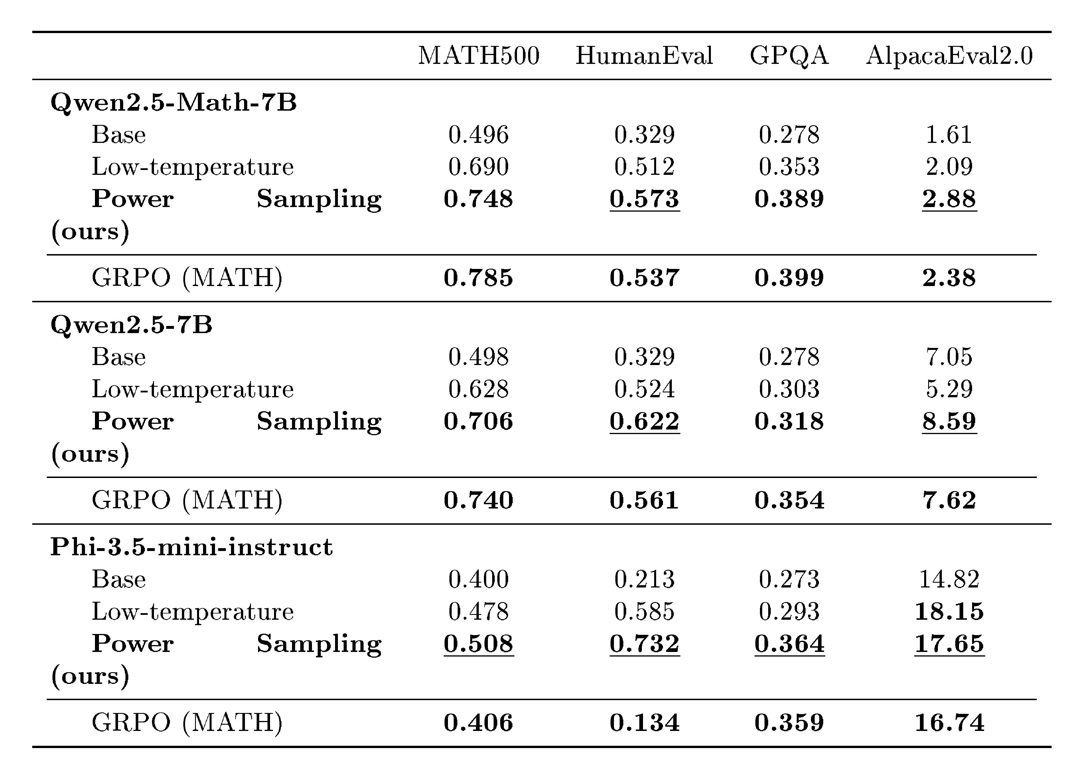
::: {caption="Table 1: Power sampling (ours) matches and even outperforms GRPO across model families and tasks. We benchmark the performance of our sampling algorithm on MATH500, HumanEval, GPQA, and AlpacaEval 2.0. We bold the scores of both our method and GRPO, and underline whenever our method outperforms GRPO. Across models, we see that power sampling is comparable to GRPO on in-domain reasoning (MATH500), and can outperform GRPO on out-of-domain tasks."}

:::

Main results.

We display our main results in Table 1. Across base models of different families, our sampling algorithm achieves massive, near-universal boosts in single-shot accuracies and scores over different reasoning and evaluation tasks that reach, e.g., up to +51.9% on HumanEval with Phi-3.5-mini and +25.2% on MATH500 with Qwen2.5-Math. In particular, on MATH500, which is in-domain for RL-posttraining, power sampling achieves accuracies that are on par with those obtained by GRPO. Furthermore, on out-of-domain reasoning, our algorithm again matches GRPO on GPQA and actually outperforms on HumanEval by up to +59.8%. Similarly, power sampling consistently outperforms on the non-verifiable AlpacaEval 2.0, suggesting a generalizability of our boosts to domains beyond verifiability.

The surprising success of this fundamentally simple yet training-free sampling algorithm underscores the latent reasoning capabilities of existing base models.

5.3 Analysis

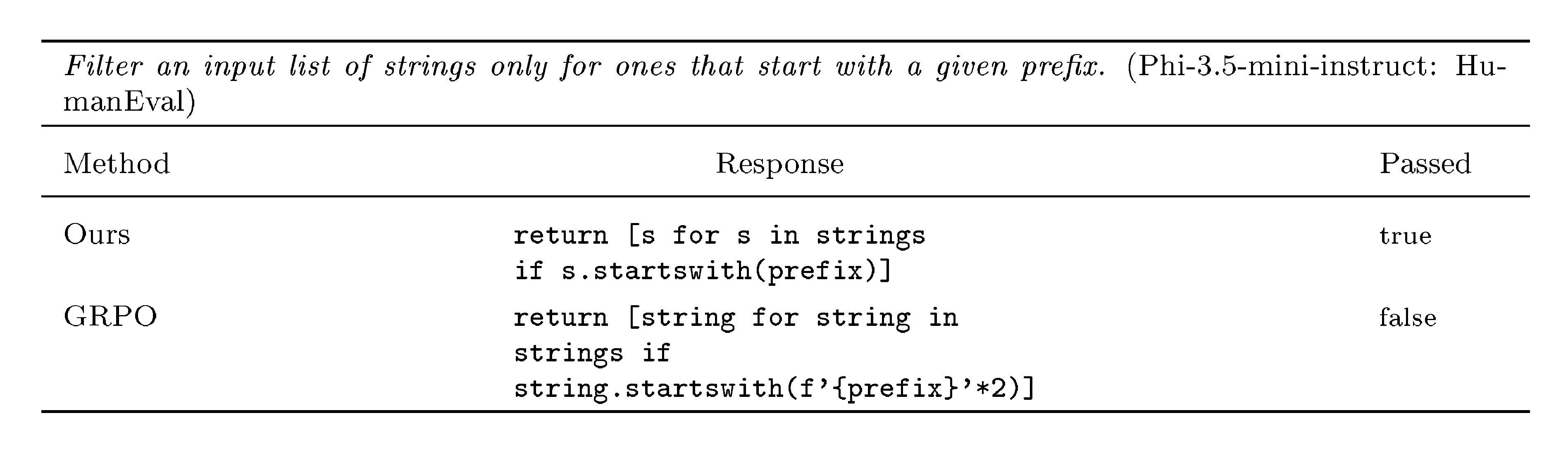
We analyze how the reasoning characteristics of power sampling relate to those of GRPO. We present an example in Table 2, with further examples in Appendix A.3.

Reasoning trace likelihoods and confidences.

By design, power sampling targets sampling higher likelihood sequences from the base model. In Figure 4, the left graph plots a histogram of the output sequence log-likelihoods (averaged by length) of the base model, power sampling, and GRPO responses on MATH500, where likelihoods are taken relative to the Qwen2.5-Math-7B base model. Our method samples from higher likelihood regions of the base model, as intended, but still maintains noticeable spread. Meanwhile, GRPO samples are heavily concentrated at the highest likelihood peak.

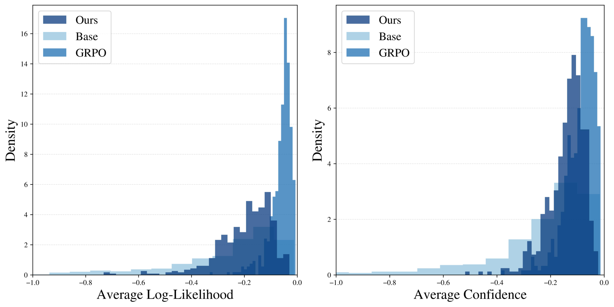
We also plot the base model confidence of MATH500 responses, defined to be the average negative entropy (uncertainty) of the next-token distributions ([11]):

$ \text{Conf}(x_{0:T}) = \frac{1}{T+1}\sum_{t=0}^T\sum_{x \in \mathcal{X}}p(x | x_{<t}) \log{p(x | x_{<t}}). $

The right plot of Figure 4 demonstrates that our method's and GRPO responses sample from similarly high confidence regions from the base model, which again correspond to regions of higher likelihood and correct reasoning.

Reasoning trace lengths.

Another defining characteristic of RL-posttraining is long-form reasoning ([1]), where samples tend to exhibit longer responses. On MATH500, Qwen2.5-Math-7B averages a response length of 600 tokens, while GRPO averages 671 tokens. Surprisingly, power sampling achieves a similar average length of 679 tokens, without explicitly being encouraged to favor longer generations. This emerges naturally from the sampling procedure.

Diversity and pass@ $k$ performance.

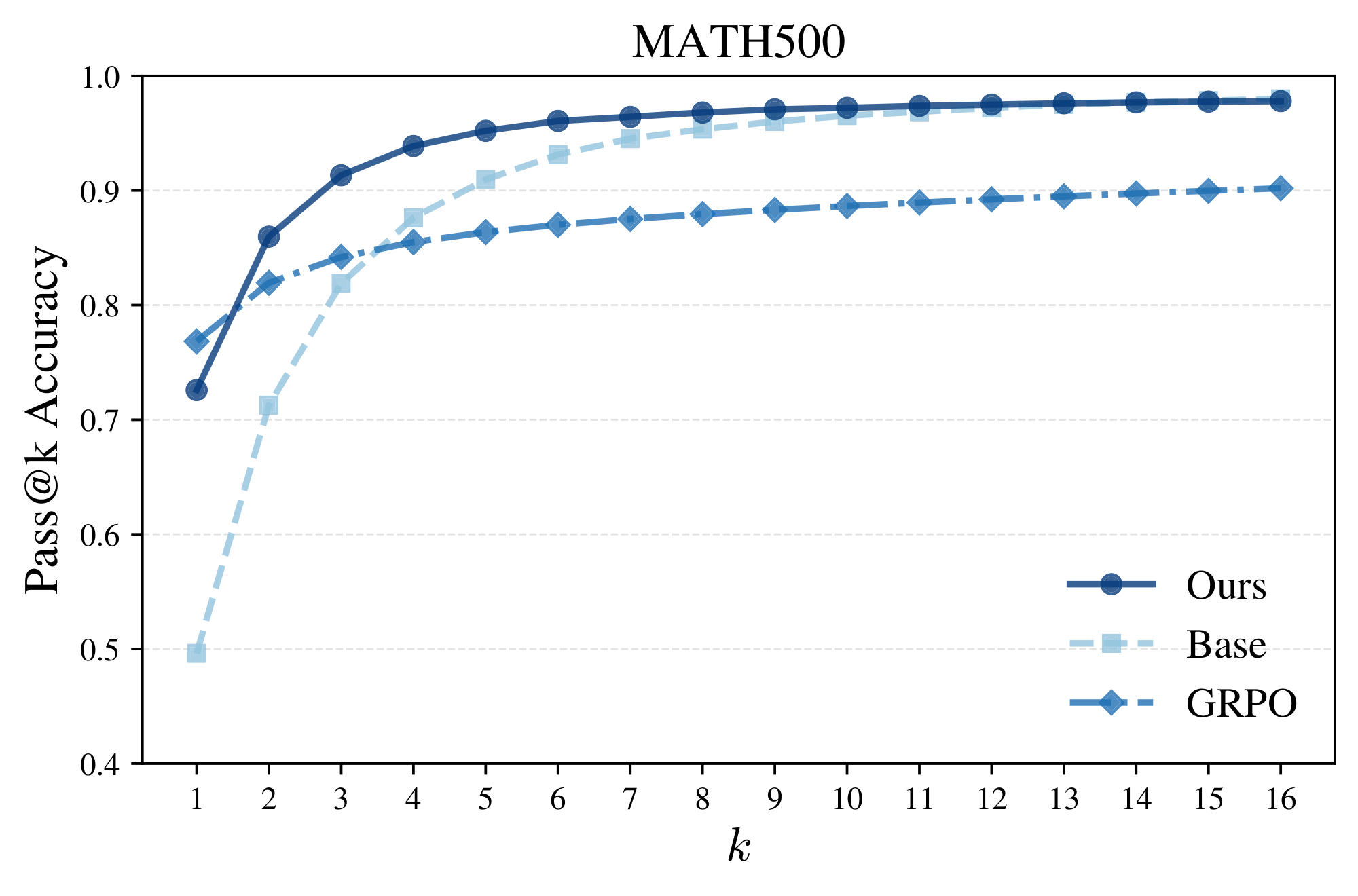
Again, notice the peaked and highly concentrated likelihoods/confidences of GRPO relative to the distributional spread of power sampling in Figure 4. This suggests GRPO exhibits a collapse in diversity while our sampler does not, aligning with the observation that RL-posttraining strongly sharpens the base model distribution at the expense of diversity ([9]). To quantify the comparative diversity of power sampling relative to GRPO, we can plot the pass@ $k$ accuracy rate, where a question is solved if at least one of $k$ samples is accurate. Figure 5 shows exactly this: unlike GRPO, whose pass@ $k$ performance tapers off for large $k$, power sampling strongly outperforms for $k > 1$. Moreover, our performance curve supersedes that of the base model until finally converging in performance. In particular, we are able to achieve GRPO-level single-shot performance without compromising multi-shot performance (see Appendix A.2 for other domains), addressing a long-standing downside to RL-posttraining.

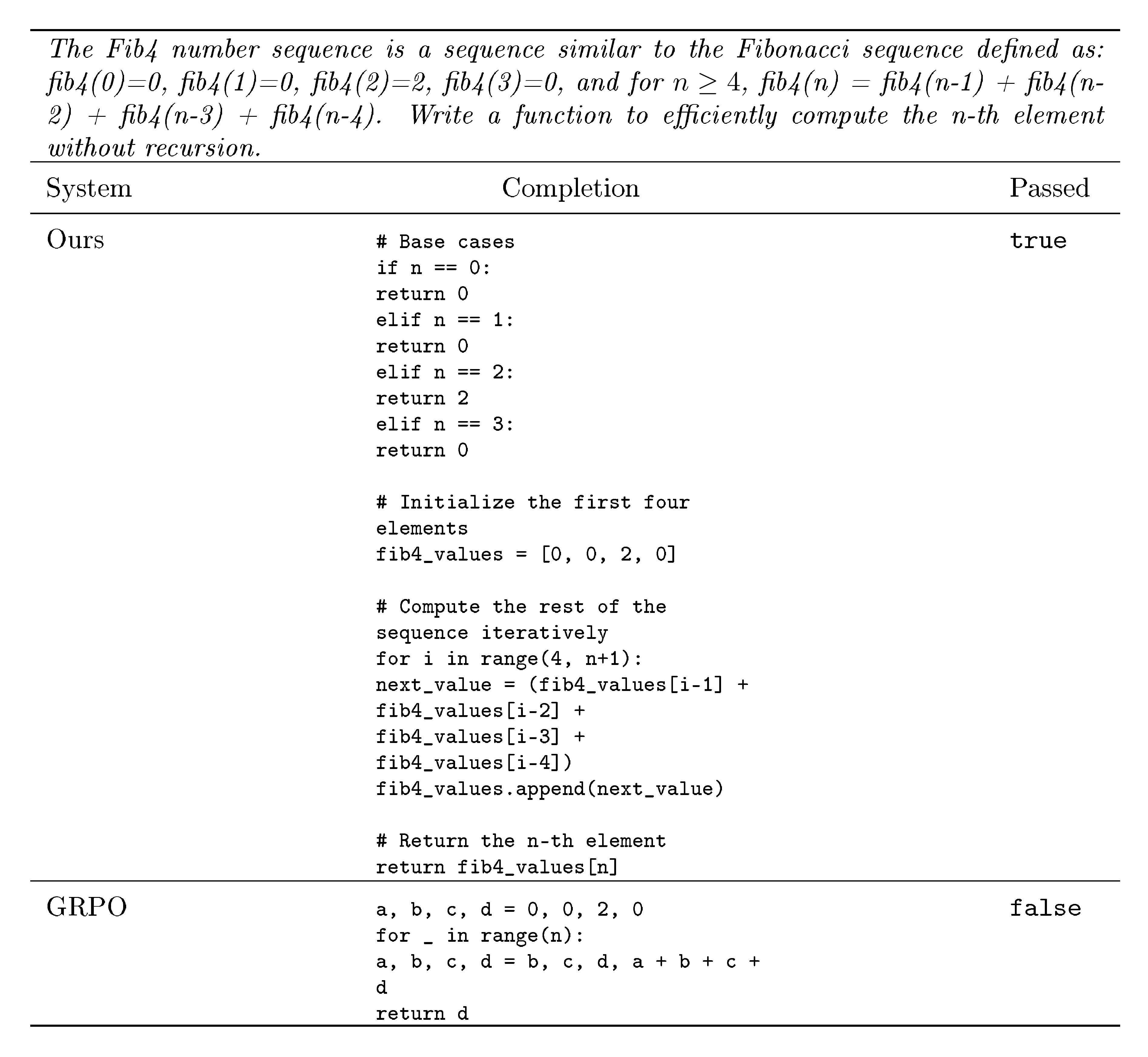
::: {caption="Table 2: Sample responses on HumanEval: Phi-3.5-mini-instruct. We present an example where our method solves a simple coding question, but GRPO does not."}

:::

The effect of power distributions.

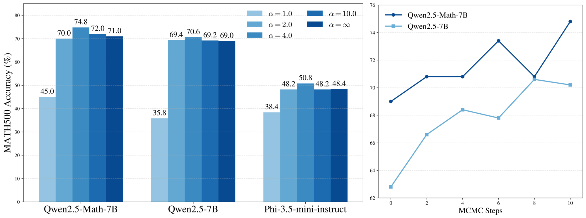
The two most important hyperparameters for power sampling are the choice of $\alpha$ and the number of MCMC (resampling) steps during sequence generation $N_{\text{MCMC}}$. At the extremes, choosing $\alpha = 1.0$ samples from the base model directly, while taking $\alpha \to \infty$ has the effect of deterministically accepting any resampled sequence that strictly increases the likelihood. Of course, even though higher base model likelihoods correlate with better reasoning (Figure 4), directly optimizing for likelihood is not necessarily optimal for reasoning, suggesting an ideal intermediate value of $\alpha$.

In Figure 6, we display MATH500 accuracies across various values of $\alpha$ and find that an intermediate $\alpha = 4.0$ outperforms other values, as expected. Noticeably, the accuracies of power sampling remain relatively stable beyond $\alpha \geq 2.0$, suggesting that power sampling in practice is relatively robust to the choice of $\alpha$.

Test-time scaling with MCMC steps.

On the other hand, $N_{\text{MCMC}}$ toggles the inference-time compute expended by our algorithm, providing a natural axis for test-time scaling. In Section 4.3 we raised the notion of a mixing time, or the number of MCMC steps required before adequately sampling from the target distribution. In our case, we expect that the fewer MCMC steps we take, the further our algorithm samples from the target $p^{\alpha}$.

We plot performance dependence on $N_{\text{MCMC}}$ in Figure 6 and notice a steady increase in accuracy until $N_{\text{MCMC}} = 10$, beyond which accuracy remains roughly stable (not plotted). The accuracy difference from using fewer MCMC steps is noticeable but no more than $3$- $4%$ between $N_{\text{MCMC}} = 2$ and $N_{\text{MCMC}} = 10$. However, the jump in accuracy by using at least two steps as opposed to none is substantial ($3$- $4$ %).

We can even compute the total amount of tokens generated by our method relative to running GRPO. From Equation (6), our sampler generates $\frac{1}{4B} \cdot {N_{\text{MCMC}}T}$ times as many tokens as standard inference to generate a sequence of length $T$. Plugging in our experimental parameters $N_{\text{MCMC}} = 10$, $T = 679$ (our average output length for MATH500) and $B = 192$, running inference with power sampling incurs a multiplier of $\textbf{8.84} \times$ the number of tokens as running standard inference. Since GRPO generates multiple rollouts per example during training, our method incurs roughly the same inference cost as one epoch of GRPO training, assuming 8 rollouts per sample with identical dataset sizes. Typically though, one GRPO epoch is still more expensive as it uses 16 rollouts and a training set that is larger than MATH500.

6. Conclusion

Section Summary: This research introduces an algorithm that draws samples straight from a basic AI model without needing extra training or outside help, delivering reasoning results in one go that match or surpass advanced techniques involving reinforcement learning. Drawing inspiration from how these methods refine probability distributions, the team targets a special "power distribution" for better reasoning, using proven sampling tricks adapted to the model's step-by-step output process, which proves effective in tests. The findings highlight that basic models have untapped potential during sampling, linking high-probability outputs to solid reasoning, and suggest that smarter use of computing power at this stage could push AI reasoning further, even into uncheckable areas.

In this work, we present an algorithm that samples directly from a base model without any additional training or access to an external signal, achieving a single-shot reasoning performance that is on par with, and sometimes even better than, that of a state-of-the-art RL-posttraining algorithm. We use the discussion of RL distribution sharpening to motivate defining the power distribution as a valuable target distribution for reasoning. Although exact power distribution sampling is intractable, we employ classic MCMC techniques alongside the sequential structure of autoregressive generation to define our power sampling algorithm, which demonstrates strong empirical performance.

Our results suggest that base model capabilities are underutilized at sampling time and point towards a close relationship between high likelihood regions of the base model and strong reasoning capabilities. Employing additional compute at sampling-time with a stronger understanding of base model capabilites offers a promising direction for expanding the scope of reasoning beyond verifiability.

7. Acknowledgments

A.K. would like to thank the Paul and Daisy Soros Foundation, NDSEG Fellowship, and Kempner Institute for their support.

Appendix

Section Summary: The appendix begins with a theoretical explanation of how power sampling favors tokens that lead to high-quality, focused future outputs, unlike low-temperature sampling, which can prioritize broader but less promising options; this is illustrated through definitions of "positive" and "negative" pivotal tokens and a mathematical proposition showing power sampling's advantages in specific scenarios. It then presents performance data across benchmarks like MATH500, GPQA, and HumanEval, where power sampling outperforms both a baseline model and another method called GRPO in generating correct answers at various sample sizes, while preserving response variety. Finally, it includes additional qualitative examples in tables comparing outputs from different approaches.

A.1 Additional Theoretical Discussion

In this section, we provide a stronger formalization of the phenomenon that power sampling downweights tokens that trap outputs in low-likelihood futures while low-temperature sampling does not.

Proposition: Informal

Power sampling upweights tokens with small support but high likelihood completions, while low-temperature sampling upweights tokens with large support but low likelihood completions.

Definition

For the rest of this section, fix a prefix $x_{0:t-1}$. We say that $x_t$ has marginal weight $\varepsilon$ under the conditional next-token distribution if $\sum_{x>t}p(x_0, \dots, x_t, \dots x_T) = \varepsilon$.

We consider a simplified model of the "critical window" or "pivotal token" phenomenon ([32, 33]), which refers to intermediate tokens that strongly influence the quality of the final generation. We differentiate between pivotal tokens that lead to high-likelihood futures vs. low-likelihood ones.

Definition

At one extreme, a pivotal token maximally induces a high-likelihood completion if it places its entire marginal weight $\varepsilon$ on one future (singular support); i.e., for only one choice of $x>t$ is $p(x_0, \dots, x_t, \dots, x_T)$ nonzero. We call such a token a

positive pivotal token.

Definition

At the other extreme, a pivotal token minimizes the likelihood of any future if its entire marginal weight $\varepsilon$ is uniformly distributed across $N$ future completions. In other words, there exist $N$ completions $x>t$ such that $p(x_0, \dots, x_t, \dots, x_T)$ are all nonzero with likelihood $\frac{\varepsilon}{N}$. We call such a token a

negative pivotal token.

Our simplified model of high and low-likelihood futures examines when positive pivotal tokens are favored over negative pivotal tokens under a given sampling distribution. In particular, we show that power sampling can upweight a positive pivotal token over a negative one even if the latter has a higher marginal weight, whereas low-temperature sampling always upweights the negative pivotal token in such a scenario.

Of course, whenever a positive pivotal token has higher marginal weight, both power sampling and low-temperature sampling will upweight it.

Proposition

Let $x_t$ be a positive pivotal token with marginal weight $\varepsilon$, and let $x_t'$ be a negative pivotal token with marginal weight $\varepsilon'$ and support $N$. Then if

$ \frac{\varepsilon'}{N^{1 - 1/\alpha}} < \varepsilon < \varepsilon', $

the future likelihood of $x_t$ is higher than any future likelihood of $x_t'$. Moreover, power sampling upweights $x_t$ over $x_t'$ while low-temperature sampling upweights $x_t'$ over $x_t$.

Proof: Since $\alpha \geq 1$, it follows that

$ \frac{\varepsilon'}{N^{1 - 1/\alpha}} > \frac{\varepsilon'}{N} $

and thus $\varepsilon > \frac{\varepsilon'}{N}$, establishing that the future completion likelihood of $x_t$ is greater than that of $x_t'$ (i.e. the assignment of positive and negative pivotal tokens is consistent).

Now, if $\varepsilon < \varepsilon'$, then under the low-temperature distribution, the relative marginal weights on $x_t$ and $x_t'$ are $\varepsilon^{\alpha}$ and $\varepsilon'^{\alpha}$, so the probability of choosing $x_t$ is downweighted relative to $x_t'$. However, for the power distribution, the relative marginal weights are $p_{\text{pow}}(x_t | x_{<t}) = \varepsilon^{\alpha}$ and $p_{\text{pow}}(x_t' | x_{<t}) = \frac{\varepsilon'^{\alpha}}{N^{\alpha - 1}}$. Then, as long as $\varepsilon^{\alpha} > \frac{\varepsilon'^{\alpha}}{N^{\alpha - 1}} \iff \varepsilon > \frac{\varepsilon'}{N^{1 - 1/{\alpha}}}$, token $x_t$ will be upweighted relative to token $x_t'$.

In other words, the marginal weight on $x_t$ can be less than the mass on $x_t'$ under $p$, but if the completion for $x_t$ has higher likelihood than any individual completion for $x_t'$, power sampling favors $x_t$ over $x_t'$.

A.2 Pass@k Accuracies over Multiple Domains

In this section, we plot the pass@ $k$ performance of power sampling, GRPO, and the base model (Qwen2.5-Math-7B) over MATH500, GPQA, and HumanEval to demonstrate that our sampling algorithm is highly performant at both single-shot and multi-shot reasoning while maintaining response diversity. Power sampling is plotted with $\alpha = 4.0$ for MATH500 and GPQA and $\alpha = 1.67$ for HumanEval (this temperature exhibits slightly better results at earlier $k$). In all cases, both in-domain and out-of-domain for GRPO, power sampling has near universally better performance than both GRPO and the base model in pass@ $k$ for $k > 1$ and matches, if not exceeds, the base model upper bound at large $k$.

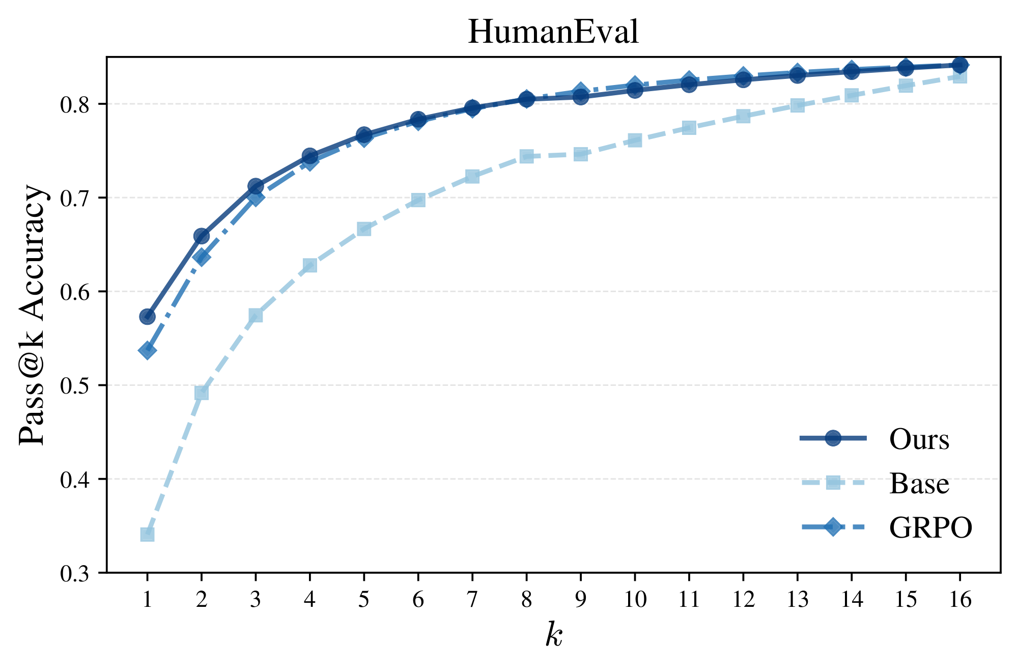
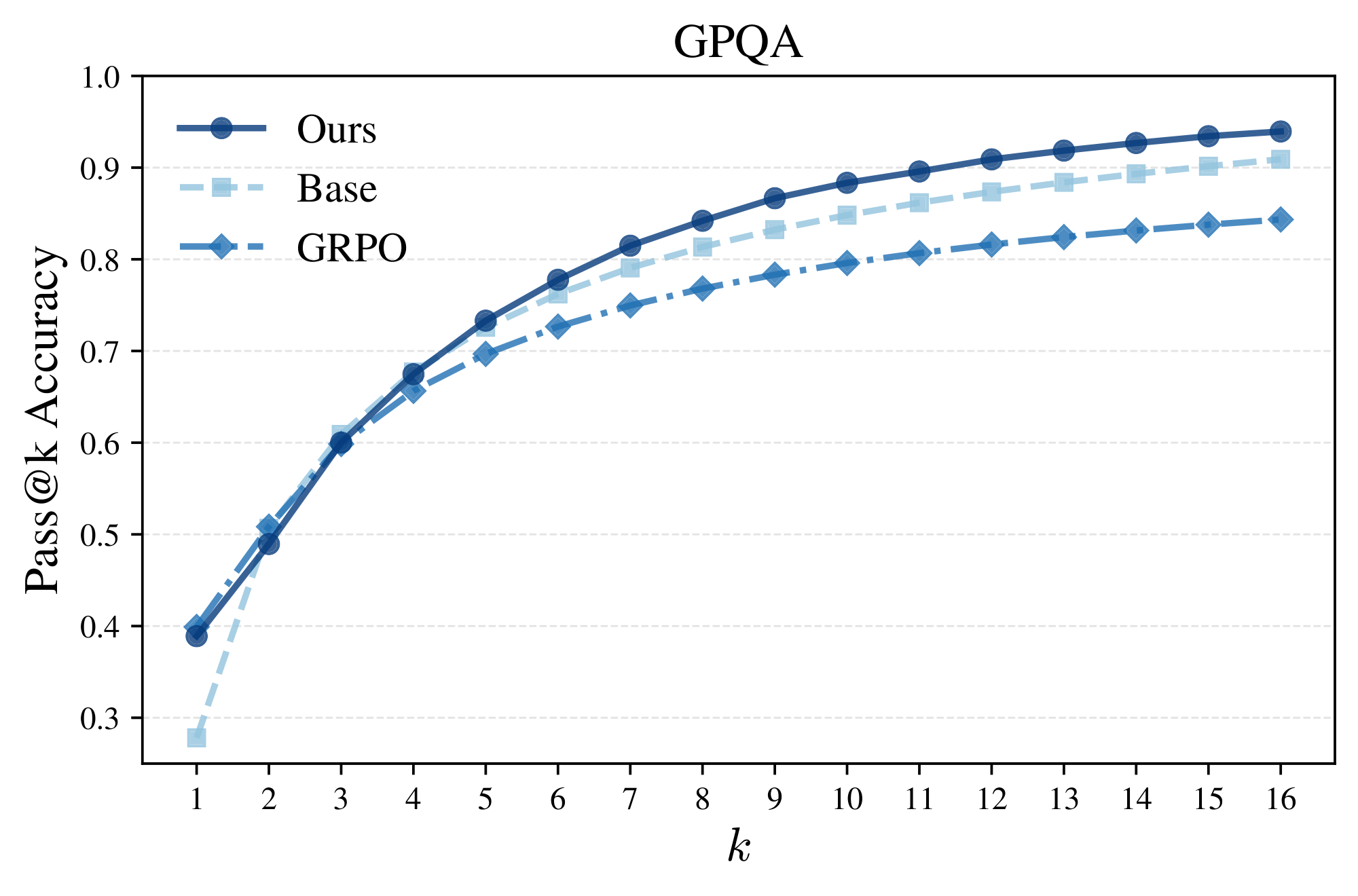
One thing to note about these plots is that the loss in diversity varies noticeably from benchmark to benchmark. MATH500 and GPQA clearly show that GRPO has a significantly lower pass@ $k$ performance and diversity even for smaller $k$, while on HumanEval GRPO exhibits better pass@ $k$ than the base model until $k = 16$. We speculate this might be due to the fact that while MATH500 and GPQA are graded on a "singular" answer, HumanEval is based on completing code where multiple solutions might be accepted, indicating a reduction in diversity may emerge but at much higher $k$.

A.3 More Qualitative Examples

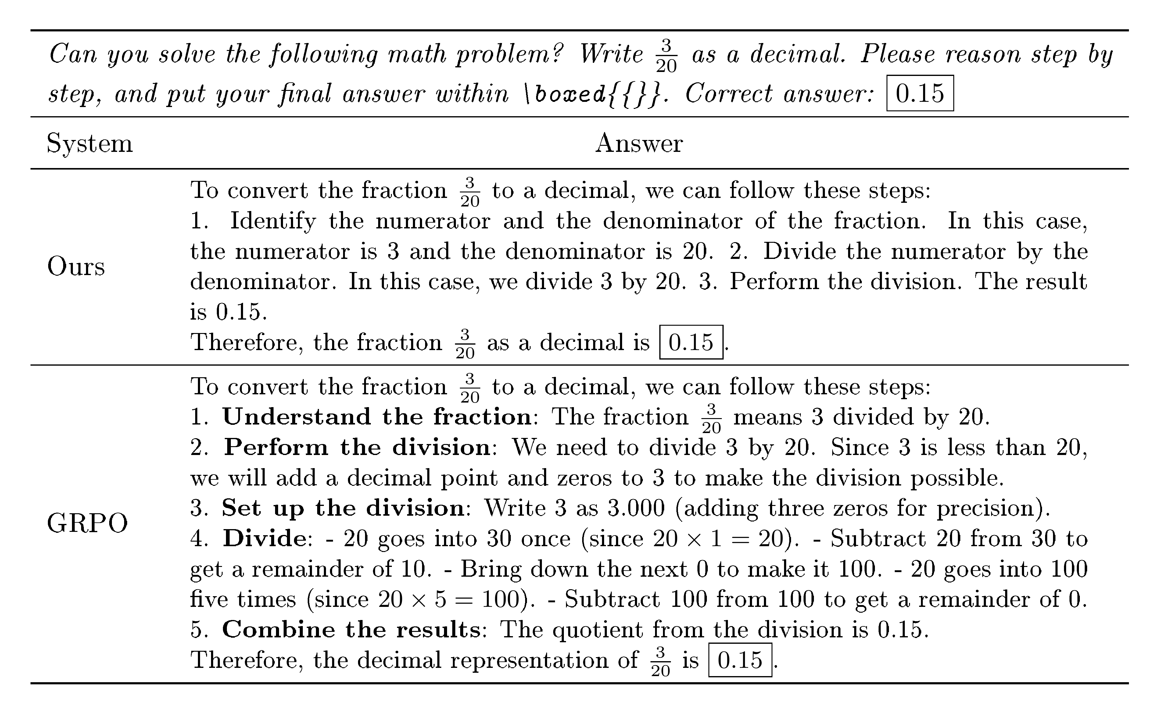
::: {caption="Table 3: Comparison on MATH500: Qwen2.5-Math-7B. We present an example where our method and GRPO are correct."}

:::

::: {caption="Table 4: HumanEval comparison on Phi-3.5-mini-instruct."}

:::

::: {caption="Table 5: MATH500 comparison between our sampling algorithm and GRPO for Qwen2.5-Math-7B. Here is an example where GRPO gets an incorrect answer, while our sampling algorithm succeeds. Our sample answer uses a distinct method altogether."}

:::

References

[1] Daya Guo, Dejian Yang, Haowei Zhang, Junxiao Song, Ruoyu Zhang, Runxin Xu, Qihao Zhu, Shirong Ma, Peiyi Wang, Xiao Bi, et al. Deepseek-r1: Incentivizing reasoning capability in LLMs via reinforcement learning. arXiv preprint arXiv:2501.12948, 2025.

[2] Jingcheng Hu, Yinmin Zhang, Qi Han, Daxin Jiang, Xiangyu Zhang, and Heung-Yeung Shum. Open-reasoner-zero: An open source approach to scaling up reinforcement learning on the base model. arXiv preprint arXiv:2503.24290, 2025.

[3] Dan Hendrycks, Collin Burns, Saurav Kadavath, Akul Arora, Steven Basart, Eric Tang, Dawn Song, and Jacob Steinhardt. Measuring mathematical problem solving with the MATH dataset. arXiv preprint arXiv:2103.03874, 2021.

[4] Yujia Li, David Choi, Junyoung Chung, Nate Kushman, Julian Schrittwieser, Rémi Leblond, Tom Eccles, James Keeling, Felix Gimeno, Agustin Dal Lago, Thomas Hubert, Peter Choy, Cyprien de Masson d'Autume, Igor Babuschkin, Xinyun Chen, Po-Sen Huang, Johannes Welbl, Sven Gowal, Alexey Cherepanov, James Molloy, Daniel Mankowitz, Esme Sutherland Robson, Pushmeet Kohli, Nando de Freitas, Koray Kavukcuoglu, and Oriol Vinyals. Competition-level code generation with AlphaCode. arXiv preprint arXiv:2203.07814, 2022.

[5] David Rein, Betty Li Hou, Asa Cooper Stickland, Jackson Petty, Richard Yuanzhe Pang, Julien Dirani, Julian Michael, and Samuel R Bowman. GPQA: A graduate-level google-proof q&a benchmark. In First Conference on Language Modeling, 2024.

[6] Andre He, Daniel Fried, and Sean Welleck. Rewarding the unlikely: Lifting GRPO beyond distribution sharpening. arXiv preprint arXiv:2506.02355, 2025.

[7] Rulin Shao, Shuyue Stella Li, Rui Xin, Scott Geng, Yiping Wang, Sewoong Oh, Simon Shaolei Du, Nathan Lambert, Sewon Min, Ranjay Krishna, Yulia Tsvetkov, Hannaneh Hajishirzi, Pang Wei Koh, and Luke Zettlemoyer. Spurious rewards: Rethinking training signals in RLVR. arXiv preprint arXiv:2506.10947, 2025.

[8] Yang Yue, Zhiqi Chen, Rui Lu, Andrew Zhao, Zhaokai Wang, Shiji Song, and Gao Huang. Does reinforcement learning really incentivize reasoning capacity in llms beyond the base model? arXiv preprint arXiv:2504.13837, 2025. URL https://arxiv.org/abs/2504.13837.

[9] Yuda Song, Julia Kempe, and Rémi Munos. Outcome-based exploration for LLM reasoning. arXiv preprint arXiv:2509.06941, 2025. URL https://arxiv.org/abs/2509.06941.

[10] Zhihong Shao, Peiyi Wang, Qihao Zhu, Runxin Xu, Junxiao Song, Xiao Bi, Haowei Zhang, Mingchuan Zhang, Y. K. Li, Y. Wu, and Daya Guo. Deepseek-math: Advancing mathematical reasoning through step-by-step exploration. arXiv preprint arXiv:2404.01140, 2024.

[11] Mihir Prabhudesai, Lili Chen, Alex Ippoliti, Katerina Fragkiadaki, Hao Liu, and Deepak Pathak. Maximizing confidence alone improves reasoning. arXiv preprint arXiv:2505.22660, 2025. URL https://arxiv.org/abs/2505.22660.

[12] Long Ouyang, Jeffrey Wu, Xu Jiang, Diogo Almeida, Carroll L. Wainwright, Pamela Mishkin, Chong Zhang, Sandhini Agarwal, Katarina Slama, Alex Ray, et al. Training language models to follow instructions with human feedback. In NeurIPS, volume 35, pages 27730–27744, 2022.

[13] Nathan Lambert, Jacob Morrison, Valentina Pyatkin, Shengyi Huang, Hamish Ivison, Faeze Brahman, Lester James V Miranda, Alisa Liu, Nouha Dziri, Shane Lyu, et al. Tülu 3: Pushing frontiers in open language model post-training. arXiv preprint arXiv:2411.15124, 2024.

[14] Weihao Zeng, Yuzhen Huang, Qian Liu, Wei Liu, Keqing He, Zejun Ma, and Junxian He. Simplerlzoo: Investigating and taming zero reinforcement learning for open base models in the wild. arXiv preprint arXiv:2503.18892, 2025. URL https://arxiv.org/abs/2503.18892.

[15] Xuandong Zhao, Zhewei Kang, Aosong Feng, Sergey Levine, and Dawn Song. Learning to reason without external rewards. arXiv preprint arXiv:2505.19590, 2025. URL https://arxiv.org/abs/2505.19590.

[16] Stephen Zhao, Rob Brekelmans, Alireza Makhzani, and Roger Grosse. Probabilistic inference in language models via twisted sequential monte carlo. arXiv preprint arXiv:2404.17546, 2024. URL https://arxiv.org/abs/2404.17546.

[17] Nicolas Chopin. Central limit theorem for sequential monte carlo methods and its application to bayesian inference. The Annals of Statistics, 32(6):2385–2411, 2004. doi:10.1214/009053604000000615. URL https://projecteuclid.org/journals/annals-of-statistics/volume-32/issue-6/Central-limit-theorem-for-sequential-Monte-Carlo-methods-and-its/10.1214/009053604000000698.full.

[18] Gonçalo R. A. Faria, Sweta Agrawal, António Farinhas, Ricardo Rei, José G. C. de Souza, and André F. T. Martins. Quest: Quality-aware metropolis-hastings sampling for machine translation. In NeurIPS, 2024. URL https://proceedings.neurips.cc/paper_files/paper/2024/file/a221d22ff6a33599142c8299c7ed06bb-Paper-Conference.pdf.

[19] Radford M. Neal. Annealed importance sampling. arXiv preprint physics/9803008, 1998. URL https://arxiv.org/abs/physics/9803008.

[20] Krzysztof Łatuszyński, Matthew T. Moores, and Timothée Stumpf-Fétizon. Mcmc for multi-modal distributions. arXiv preprint arXiv:2501.05908, 2025. URL https://arxiv.org/abs/2501.05908v1.

[21] Yilun Du, Conor Durkan, Robin Strudel, Joshua B Tenenbaum, Sander Dieleman, Rob Fergus, Jascha Sohl-Dickstein, Arnaud Doucet, and Will Sussman Grathwohl. Reduce, reuse, recycle: Compositional generation with energy-based diffusion models and mcmc. In International conference on machine learning, pages 8489–8510. PMLR, 2023.

[22] Sunwoo Kim, Minkyu Kim, and Dongmin Park. Test-time alignment of diffusion models without reward over-optimization. arXiv preprint arXiv:2501.05803, 2025. URL https://arxiv.org/abs/2501.05803.

[23] Aayush Karan, Kulin Shah, and Sitan Chen. Reguidance: A simple diffusion wrapper for boosting sample quality on hard inverse problems. arXiv preprint arXiv:2506.10955, 2025. URL https://arxiv.org/abs/2506.10955.

[24] Yanwei Wang, Lirui Wang, Yilun Du, Balakumar Sundaralingam, Xuning Yang, Yu-Wei Chao, Claudia Pérez-D’Arpino, Dieter Fox, and Julie Shah. Inference-time policy steering through human interactions. In 2025 IEEE International Conference on Robotics and Automation (ICRA), pages 15626–15633. IEEE, 2025.

[25] Lingkai Kong, Yuanqi Du, Wenhao Mu, Kirill Neklyudov, Valentin De Bortoli, Dongxia Wu, Haorui Wang, Aaron M. Ferber, Yian Ma, Carla P. Gomes, and Chao Zhang. Diffusion models as constrained samplers for optimization with unknown constraints. In Yingzhen Li, Stephan Mandt, Shipra Agrawal, and Emtiyaz Khan, editors, Proceedings of The 28th International Conference on Artificial Intelligence and Statistics, volume 258 of Proceedings of Machine Learning Research, pages 4582–4590. PMLR, 2025. URL https://proceedings.mlr.press/v258/kong25b.html.

[26] Xiangcheng Zhang, Haowei Lin, Haotian Ye, James Zou, Jianzhu Ma, Yitao Liang, and Yilun Du. Inference-time scaling of diffusion models through classical search. arXiv preprint arXiv:2505.23614, 2025.

[27] Malcolm Sambridge. A parallel tempering algorithm for probabilistic sampling and optimization. Geophysical Journal International, 196(1):357–374, 2014. doi:10.1093/gji/ggt374. URL https://academic.oup.com/gji/article/196/1/357/585739.

[28] Marta Skreta, Tara Akhound-Sadegh, Viktor Ohanesian, Roberto Bondesan, Alán Aspuru-Guzik, Arnaud Doucet, Rob Brekelmans, Alexander Tong, and Kirill Neklyudov. Feynman-kac correctors in diffusion: Annealing, guidance, and product of experts. arXiv preprint arXiv:2503.02819, 2025. URL https://arxiv.org/abs/2503.02819.

[29] Yanbo Xu, Yu Wu, Sungjae Park, Zhizhuo Zhou, and Shubham Tulsiani. Temporal score rescaling for temperature sampling in diffusion and flow models. arXiv preprint arXiv:2510.01184, 2025. URL https://arxiv.org/abs/2510.01184.

[30] Tomas Geffner, Kieran Didi, Zuobai Zhang, Danny Reidenbach, Zhonglin Cao, Jason Yim, Mario Geiger, Christian Dallago, Emine Kucukbenli, and Arash Vahdat. Proteina: Scaling flow-based protein structure generative models. arXiv preprint arXiv:2503.00710, 2025. URL https://arxiv.org/abs/2503.00710.

[31] Pei-Hsin Wang, Sheng-Iou Hsieh, Shih-Chieh Chang, Yu-Ting Chen, Jia-Yu Pan, Wei Wei, and Da-Chang Juan. Contextual temperature for language modeling. arXiv preprint arXiv:2012.13575, 2020. URL https://arxiv.org/abs/2012.13575.

[32] Marvin Li, Aayush Karan, and Sitan Chen. Blink of an eye: A simple theory for feature localization in generative models. arXiv preprint arXiv:2502.00921, 2025. URL https://arxiv.org/abs/2502.00921.

[33] Marah Abdin, Jyoti Aneja, Harkirat Behl, Sébastien Bubeck, Ronen Eldan, Suriya Gunasekar, Michael Harrison, Russell J. Hewett, Mojan Javaheripi, Piero Kauffmann, James R. Lee, Yin Tat Lee, Yuanzhi Li, Weishung Liu, Caio C. T. Mendes, Anh Nguyen, Eric Price, Gustavo de Rosa, Olli Saarikivi, Adil Salim, Shital Shah, Xin Wang, Rachel Ward, Yue Wu, Dingli Yu, Cyril Zhang, and Yi Zhang. Phi-4 technical report. arXiv preprint arXiv:2412.08905, 2024. URL https://arxiv.org/abs/2412.08905.

[34] Nicholas Metropolis, Arianna W. Rosenbluth, Marshall N. Rosenbluth, Augusta H. Teller, and Edward Teller. Equation of state calculations by fast computing machines. Journal of Chemical Physics, 21(6):1087–1092, 1953. doi:10.1063/1.1699114.

[35] Radford M Neal. Probabilistic inference using markov chain monte carlo methods. Department of Computer Science, University of Toronto (review paper / technical report), 1993.

[36] Reza Gheissari, Eyal Lubetzky, and Yuval Peres. Exponentially slow mixing in the mean-field swendsen–wang dynamics. arXiv preprint arXiv:1702.05797, 2017.

[37] Afonso S. Bandeira, Antoine Maillard, Richard Nickl, and Sven Wang. On free energy barriers in gaussian priors and failure of cold start mcmc for high-dimensional unimodal distributions. arXiv preprint arXiv:2209.02001, 2022. URL https://arxiv.org/abs/2209.02001.

[38] Scott C. Schmidler and Dawn B. Woodard. Lower bounds on the convergence rates of adaptive mcmc methods. Technical report, Duke University / Cornell University, 2013. URL https://www2.stat.duke.edu/~scs/Papers/AdaptiveLowerBounds_AS.pdf.

[39] Hunter Lightman, Vineet Kosaraju, Yura Burda, Harri Edwards, Bowen Baker, Teddy Lee, Jan Leike, John Schulman, Ilya Sutskever, and Karl Cobbe. Let's verify step by step. In The Twelfth International Conference on Learning Representations, 2024. URL https://openreview.net/forum?id=v8L0pN6EOi.

[40] M. Chen, J. Tworek, H. Jun, Q. Yuan, H. P. de Oliveira Pinto, J. Kaplan, H. Edwards, Y. Burda, N. Joseph, G. Brockman, A. Ray, R. Puri, G. Krueger, M. Petrov, H. Khlaaf, G. Sastry, P. Mishkin, B. Chan, S. Gray, N. Ryder, M. Pavlov, A. Power, L. Kaiser, M. Bavarian, C. Winter, P. Tillet, F. P. Such, D. Cummings, M. Plappert, F. Chantzis, E. Barnes, A. Herbert-Voss, W. H. Guss, A. Nichol, A. Paino, N. Tezak, J. Tang, I. Babuschkin, S. Balaji, S. Jain, W. Saunders, C. Hesse, A. N. Carr, J. Leike, J. Achiam, V. Misra, E. Morikawa, A. Radford, M. Knight, M. Brundage, M. Murati, K. Mayer, P. Welinder, B. McGrew, D. Amodei, S. McCandlish, I. Sutskever, and W. Zaremba. Evaluating large language models trained on code. CoRR, abs/2107.03374, 2021. URL https://arxiv.org/abs/2107.03374.

[41] Yann Dubois, Balázs Galambosi, Percy Liang, and Tatsunori B. Hashimoto. Length-controlled alpacaeval: A simple way to debias automatic evaluators. arXiv preprint arXiv:2404.04475, 2024. URL https://arxiv.org/abs/2404.04475.