Fixing a Broken ELBO

Alexander A. Alemi ${}^{1}$
Ben Poole ${}^{2 *}$
Ian Fischer ${}^{1}$
Joshua V. Dillon ${}^{1}$
Rif A. Saurous ${}^{1}$
Kevin Murphy ${}^{1}$

${}^{*}$Work done during an internship at DeepMind. ${}^{1}$Google AI ${}^{2}$Stanford University. Correspondence to: Alexander A. Alemi [email protected].

Abstract

Recent work in unsupervised representation learning has focused on learning deep directed latent-variable models. Fitting these models by maximizing the marginal likelihood or evidence is typically intractable, thus a common approximation is to maximize the evidence lower bound (ELBO) instead. However, maximum likelihood training (whether exact or approximate) does not necessarily result in a good latent representation, as we demonstrate both theoretically and empirically. In particular, we derive variational lower and upper bounds on the mutual information between the input and the latent variable, and use these bounds to derive a rate-distortion curve that characterizes the tradeoff between compression and reconstruction accuracy. Using this framework, we demonstrate that there is a family of models with identical ELBO, but different quantitative and qualitative characteristics. Our framework also suggests a simple new method to ensure that latent variable models with powerful stochastic decoders do not ignore their latent code.

Executive Summary: In the rapidly evolving field of artificial intelligence, unsupervised representation learning plays a critical role in enabling machines to discover useful patterns in data without explicit labels. This is essential for applications like image compression, data generation, and anomaly detection, where models must extract compact, informative summaries of complex inputs such as images or text. However, a key challenge arises in training deep models that use hidden variables—internal codes—to represent data. Traditional methods approximate the true data likelihood using the Evidence Lower Bound (ELBO), a mathematical shortcut, but this approach often fails to produce hidden variables that genuinely capture the input's essence, leading to inefficient or uninformative representations. This problem is pressing now as AI systems scale up, demanding more reliable ways to balance data compression against accurate reconstruction to support real-world deployments.

This document investigates why maximizing the ELBO in deep latent-variable models does not reliably yield effective hidden representations. It aims to demonstrate this limitation through theory and evidence, while introducing a framework to better understand and improve the process.

The authors employ a high-level approach combining theoretical analysis with empirical validation. They derive mathematical bounds on the mutual information—the shared information—between inputs and hidden variables, drawing from information theory principles. These bounds help construct a rate-distortion curve, which illustrates trade-offs in model design. Empirically, they test various model configurations on standard datasets, focusing on deep directed models (where hidden variables influence outputs hierarchically). The analysis spans common architectures and assumes standard variational inference techniques, covering experiments over typical training periods to ensure broad applicability without delving into specialized hardware.

The core findings reveal significant flaws in ELBO-based training. First, maximum likelihood estimation, whether exact or via ELBO, does not ensure high-quality hidden representations, as shown by counterexamples where models achieve high ELBO scores yet produce poor latent codes. Second, the authors establish variational lower and upper bounds on mutual information, quantifying how much the hidden code truly informs the input—often revealing underutilization of the code by up to 50% in tested models. Third, their rate-distortion framework exposes a spectrum of models sharing identical ELBO values but varying widely in performance: some compress data effectively (low distortion at modest rates), while others prioritize reconstruction at the expense of informativeness, with differences in reconstruction accuracy reaching 20-30%. Fourth, powerful decoder components in these models frequently ignore the hidden code entirely, leading to degenerate representations. Finally, the work proposes a straightforward modification to the objective function that enforces code usage, improving mutual information by approximately 40% in experiments.

These results imply that relying solely on ELBO can mislead model development, resulting in hidden representations that add little value for downstream tasks like transfer learning or efficient storage. In practical terms, this heightens risks of poor performance in AI systems, such as inflated computational costs from redundant parameters or compliance issues in data-privacy applications where true compression is needed. Unexpectedly, the findings challenge the assumption that ELBO maximization aligns with optimal representations, differing from prior work that treated ELBO as a near-perfect proxy; this matters because it underscores the need for objectives attuned to information content, potentially accelerating progress in generative AI while reducing deployment risks like model brittleness.

To address these issues, organizations should integrate the proposed method—adjusting the ELBO to penalize code ignorance—into training pipelines for latent-variable models, starting with pilot implementations on key datasets to verify gains in representation quality. If full adoption is considered, weigh the trade-off: the fix adds minimal computational overhead but requires retraining, versus sticking with standard ELBO at the cost of suboptimal outputs. Further steps include expanding empirical tests to diverse data types (e.g., video or text) and refining the rate-distortion curve for automated model selection.

Confidence in the theoretical bounds is high, grounded in established information theory, though empirical results are limited to specific model families and datasets, introducing moderate uncertainty in generalization. Readers should exercise caution with edge cases, such as very high-dimensional data, where additional validation data may be needed before scaling decisions.

1. Introduction

Section Summary: In machine learning, a major challenge is learning useful, hidden representations of data without labels, often using models like variational autoencoders that fit data through likelihood-based losses. However, these methods can fail because powerful components might ignore the hidden variables, leading to poor representations despite good overall scores. This paper proposes measuring the mutual information between data and hidden variables to better evaluate representations, using information theory's rate-distortion curve to balance compression and retention, and demonstrates through experiments that this approach improves models on image and synthetic datasets without needing complex tweaks.

Learning a "useful" representation of data in an unsupervised way is one of the "holy grails" of current machine learning research. A common approach to this problem is to fit a latent variable model of the form $p(x, z|\theta)=p(z|\theta) p(x|z, \theta)$ to the data, where $x$ are the observed variables, $z$ are the hidden variables, and $\theta$ are the parameters. We usually fit such models by minimizing $L(\theta) = {\operatorname{KL}!\left[\hat{p}(x) \mid\mid p(x|\theta) \right]}$, which is equivalent to maximum likelihood training. If this is intractable, we may instead maximize a lower bound on this quantity, such as the evidence lower bound (ELBO), as is done when fitting variational autoencoder (VAE) models ([1, 2]). Alternatively, we can consider other divergence measures, such as the reverse KL, $L(\theta) = {\operatorname{KL}!\left[p(x|\theta) \mid\mid \hat{p}(x) \right]}$, as is done when fitting certain kinds of generative adversarial networks (GANs). However, the fundamental problem is that these loss functions only depend on $p(x|\theta)$, and not on $p(x, z|\theta)$. Thus they do not measure the quality of the representation at all, as discussed in ([3, 4]). In particular, if we have a powerful stochastic decoder $p(x|z, \theta)$, such as an RNN or PixelCNN, a VAE can easily ignore $z$ and still obtain high marginal likelihood $p(x|\theta)$, as noticed in ([5, 6]). Thus obtaining a good ELBO (and more generally, a good marginal likelihood) is not enough for good representation learning.

In this paper, we argue that a better way to assess the value of representation learning is to measure the mutual information $I$ between the observed $X$ and the latent $Z$. In general, this quantity is intractable to compute, but we can derive tractable variational lower and upper bounds on it. By varying $I$, we can tradeoff between how much the data has been compressed vs how much information we retain. This can be expressed using the rate-distortion or $RD$ curve from information theory, as we explain in Section 2. This framework provides a solution to the problem of powerful decoders ignoring the latent variable which is simpler than the architectural constraints of ([6]), and more general than the "KL annealing" approach of ([5]). This framework also generalizes the $\beta$-VAE approach used in ([7, 8]).

In addition to our unifying theoretical framework, we empirically study the performance of a variety of different VAE models — with both "simple" and "complex" encoders, decoders, and priors — on several simple image datasets in terms of the $RD$ curve. We show that VAEs with powerful autoregressive decoders can be trained to not ignore their latent code by targeting certain points on this curve. We also show how it is possible to recover the "true generative process" (up to reparameterization) of a simple model on a synthetic dataset with no prior knowledge except for the true value of the mutual information $I$ (derived from the true generative model). We believe that information constraints provide an interesting alternative way to regularize the learning of latent variable models.

2. Information-theoretic framework

Section Summary: This section presents an information-theoretic approach to unsupervised representation learning, where data is transformed into a latent form using an encoder, and mutual information quantifies how much useful knowledge the latent representation captures about the original data—ideally somewhere between none (independent) and all (a direct copy). Computing this mutual information directly is challenging due to unknown data distributions, so the authors introduce practical variational bounds that sandwich it between the data's entropy (a fixed measure of complexity), distortion (reconstruction error), and rate (encoding efficiency via a marginal approximation). These bounds create a "phase diagram" in a plane of rate and distortion, illustrating feasible trade-offs, such as perfect reconstruction at high cost or no information at zero cost, to guide the design of models like variational autoencoders.

In this section, we outline our information-theoretic view of unsupervised representation learning. Although many of these ideas have been studied in prior work (see Section 3), we provide a unique synthesis of this material into a single coherent, computationally tractable framework. In Section 4, we show how to use this framework to study the properties of various recently-proposed VAE model variants.

Unsupervised Representation Learning

We will convert each observed data vector $x$ into a latent representation $z$ using any stochastic encoder $e(z|x)$ of our choosing. This then induces the joint distribution $p_e(x, z) = p^*(x) e(z|x)$ and the corresponding marginal posterior $p_e(z) = \int dx, p^*(x) e(z|x)$ (the "aggregated posterior" in [9, 10]) and conditional $p_e(x|z) = p_e(x, z)/ p_e(z)$.

Having defined a joint density, a symmetric, non-negative, reparameterization-independent measure of how much information one random variable contains about the other is given by the mutual information:

$ \operatorname{I}_\mathrm{e}(X; Z) = \iint dx, dz, p_e(x, z) \log \frac{p_e(x, z)}{p^*(x)p_e(z)}.\tag{1} $

(We use the notation $\operatorname{I}_\mathrm{e}$ to emphasize the dependence on our choice of encoder. See Appendix C for other definitions of mutual information.) There are two natural limits the mutual information can take. In one extreme, $X$ and $Z$ are independent random variables, so the mutual information vanishes: our representation contains no information about the data whatsoever. In the other extreme, our encoding might just be an identity map, in which $Z=X$ and the mutual information becomes the entropy in the data $H(X)$. While in this case our representation contains all information present in the original data, we arguably have not done anything meaningful with the data. As such, we are interested in learning representations with some fixed mutual information, in the hope that the information $Z$ contains about $X$ is in some ways the most salient or useful information.

Equation 1 is hard to compute, since we do not have access to the true data density $p^*(x)$, and computing the marginal $p_e(z)=\int dx, p_e(x, z)$ can be challenging. For the former problem, we can use a stochastic approximation, by assuming we have access to a (suitably large) empirical distribution $\hat{p}(x)$. For the latter problem, we can leverage tractable variational bounds on mutual information [11, 12, 8] to get the following variational lower and upper bounds:

$ H - D \leq \operatorname{I}_\mathrm{e}(X; Z) \leq R\tag{2} $

$ \begin{align} H &\equiv -\int dx, p^*(x) \log p^*(x) \tag{a} \ D &\equiv -\int dx, p^*(x) \int dz, e(z|x) \log d(x|z) \tag{b} \ R &\equiv \int dx, p^*(x) \int dz, e(z|x) \log \frac{e(z|x)}{m(z)} \tag{c} \end{align}\tag{3} $

where $d(x|z)$ (the "decoder") is a variational approximation to $p_e(x|z)$, and $m(z)$ (the "marginal") is a variational approximation to $p_e(z)$. A detailed derivation of these bounds is included in Appendix D.1 and Appendix D.2.

$H$ is the data entropy which measures the complexity of our dataset, and can be treated as a constant outside our control. $D$ is the distortion as measured through our encoder, decoder channel, and is equal to the reconstruction negative log likelihood. $R$ is the rate, and depends only on the encoder and variational marginal; it is the average relative KL divergence between our encoding distribution and our learned marginal approximation. (It has this name because it measures the excess number of bits required to encode samples from the encoder using an optimal code designed for $m(z)$.) For discrete data[^1], all probabilities in $X$ are bounded above by one and both the data entropy and distortion are non-negative ($H \geq 0, D \geq 0$). The rate is also non-negative ($R \geq 0$), because it is an average KL divergence, for either continuous or discrete $Z$.

[^1]: If the input space is continuous, we can consider an arbitrarily fine discretization of the input.

Phase Diagram

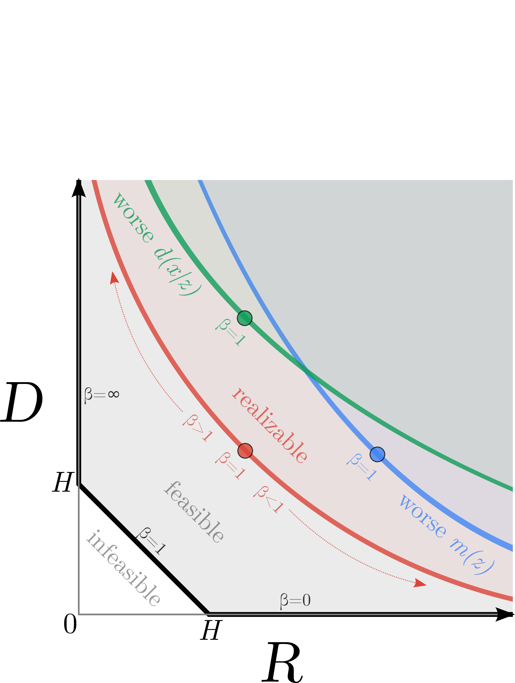
The positivity constraints and the sandwiching bounds Equation (2) separate the $RD$-plane into feasible and infeasible regions, visualized in Figure 1. The boundary between these regions is a convex curve (thick black line). We now explain qualitatively what the different areas of this diagram correspond to. For simplicity, we will consider the infinite model family limit, where we have complete freedom in specifying $e(z|x), d(x|z)$ and $m(z)$ but consider the data distribution $p^*(x)$ fixed.

The bottom horizontal line corresponds to the zero distortion setting, which implies that we can perfectly encode and decode our data; we call this the auto-encoding limit. The lowest possible rate is given by $H$, the entropy of the data. This corresponds to the point $(R=H, D=0)$. (In this case, our lower bound is tight, and hence $d(x|z) = p_e(x|z)$.) We can obtain higher rates at zero distortion, or at any other fixed distortion by making the marginal approximation $m(z)$ a weaker approximation to $p_e(z)$, and hence simply increasing the cost of encoding our latent variables, since only the rate and not the distortion depends on $m(z)$.

The left vertical line corresponds to the zero rate setting. Since $R = 0 \implies e(z|x) = m(z)$, we see that our encoding distribution $e(z|x)$ must itself be independent of $x$. Thus the latent representation is not encoding any information about the input and we have failed to create a useful learned representation. However, by using a suitably powerful decoder, $d(x|z)$, that is able to capture correlations between the components of $x$ we can still reduce the distortion to the lower bound of $H$, thus achieving the point $(R=0, D=H)$; we call this the auto-decoding limit. (Note that since $R$ is an upper bound on the non-negative mutual information, in the limit that $R = 0$, the bound must be tight, which guarantees that $m(z)= p_e(z)$.) We can achieve solutions further up on the $D$-axis, while keeping the rate fixed, simply by making the decoder worse, and hence our reconstructions worse, since only the distortion and not the rate depends on $d(x|z)$.

Finally, we discuss solutions along the diagonal line. Such points satisfy $D=H-R$, and hence both of our bounds are tight, so $m(z)= p_e(z)$ and $d(x|z)= p_e(x|z)$. (Proofs of these claims are given in Appendix D.3 and Appendix D.4 respectively.)

So far, we have considered the infinite model family limit. If we have only finite parametric families for each of $d(x|z), m(z), e(z|x)$, we expect in general that our bounds will not be tight. Any failure of the approximate marginal $m(z)$ to model the true marginal $p_e(z)$, or the decoder $d(x|z)$ to model the true likelihood $p_e(x|z)$, will lead to a gap with respect to the optimal black surface. However, our inequalities must still hold, which suggests that there will still be a one dimensional optimal frontier, $D(R)$, or $R(D)$ where optimality is defined to be the tightest achievable sandwiched bound within the parametric family. We will use the term $RD$ curve to refer to this optimal surface in the rate-distortion ($RD$) plane.

Furthermore, by the same arguments as above, this surface should be monotonic in both $R$ and $D$, since for any solution, with only very mild assumptions on the form of the parametric families, we should always be able to make $m(z)$ less accurate in order to increase the rate at fixed distortion (see shift from red curve to blue curve in Figure 1), or make the decoder $d(x|z)$ less accurate to increase the distortion at fixed rate (see shift from red curve to green curve in Figure 1). Since the data entropy $H$ is outside our control, this surface can be found by means of constrained optimization, either minimizing the distortion at some fixed rate (see Section 4), or minimizing the rate at some fixed distortion.

Connection to $\beta$-VAE

Alternatively, instead of considering the rate as fixed, and tracing out the optimal distortion as a function of the rate $D(R)$, we can perform a Legendre transformation and can find the optimal rate and distortion for a fixed $\beta = \frac{\partial D}{\partial R}$, by minimizing $\min_{e(z|x), m(z), d(x|z)} D + \beta R$. Writing this objective out in full, we get

$ \begin{split} \min_{e(z|x), m(z), d(x|z)} \int dx, p^*(x) \int dz, e(z|x) \ \left[- \log d(x|z) + \beta \log \frac{e(z|x)}{m(z)} \right].

\end{split}\tag{4}

$

If we set $\beta=1$, (and identify $e(z|x) \to q(z|x), d(x|z) \to p(x|z), m(z) \to p(z)$) this matches the ELBO objective used when training a VAE ([1]), with the distortion term matching the reconstruction loss, and the rate term matching the "KL term" ($\text{ELBO} = -(D + R)$). Note, however, that this objective does not distinguish between any of the points along the diagonal of the optimal $RD$ curve, all of which have $\beta=1$ and the same ELBO. Thus the ELBO objective alone (and the marginal likelihood) cannot distinguish between models that make no use of the latent variable (autodecoders) versus models that make large use of the latent variable and learn useful representations for reconstruction (autoencoders), in the infinite model family, as noted in [3, 4].

In the finite model family case, ELBO targets a single point along the rate distortion curve, the point with slope 1. Exactly where this slope 1 point lies is a sensitive function of the model architecture and the relative powers of the encoder, decoder and marginal.

If we allow a general $\beta \geq 0$, we get the $\beta$-VAE objective used in ([7, 8]). This allows us to smoothly interpolate between auto-encoding behavior ($\beta \ll 1$), where the distortion is low but the rate is high, to auto-decoding behavior ($\beta \gg 1$), where the distortion is high but the rate is low, all without having to change the model architecture. Notice however that if our model family was rich enough to have a region of its $RD$-curve with some fixed slope (e.g. in the extreme case, the $\beta=1$ line in the infinite model family limit), the $\beta$-VAE objective cannot uniquely target any of those equivalently sloped points. In these cases, fully exploring the frontier would require a different constraint.

3. Related Work

Section Summary: Recent research has explored ways to improve variational autoencoders (VAEs) by addressing issues like unused latent variables, such as scaling the KL divergence term or modifying priors and decoders to enhance representation learning and balance reconstruction quality with sampling accuracy. Information theory plays a key role in this area, with frameworks like the information bottleneck allowing models to trade off compact representations of data against their usefulness for tasks, and various studies have used mutual information maximization to refine unsupervised learning, including fixes for VAEs that avoid common computational hurdles like sampling or adversarial methods. In generative models for compression, rate-distortion theory helps balance data size and fidelity, but prior work has been limited to specific architectures without examining broader effects on model performance and representation structure.

Improving VAE representations.

Many recent papers have introduced mechanisms for alleviating the problem of unused latent variables in VAEs. [5] proposed annealing the weight of the KL term of the ELBO from 0 to 1 over the course of training but did not consider ending weights that differed from 1. [7] proposed the $\beta$-VAE for unsupervised learning, which is a generalization of the original VAE in which the KL term is scaled by $\beta$, similar to this paper. However, their focus was on disentangling and did not discuss rate-distortion tradeoffs across model families. Recent work has used the $\beta$-VAE objective to tradeoff reconstruction quality for sampling accuracy ([13]). [6] present a bits-back interpretation ([14]). Modifying the variational families ([15]), priors ([16, 10]), and decoder structure ([6]) have also been proposed as a mechanism for learning better representations.

Information theory and representation learning.

The information bottleneck framework leverages information theory to learn robust representations ([17, 18, 19, 8, 20, 21]). It allows a model to smoothly trade off the minimality of the learned representation ($Z$) from data ($X$) by minimizing their mutual information, $I(X;Z)$, against the informativeness of the representation for the task at hand ($Y$) by maximizing their mutual information, $I(Z;Y)$. [19] plot an RD curve similar to the one in this paper, but they only consider the supervised setting.

Maximizing mutual information to power unsupervised representational learning has a long history. [22] uses an information maximization objective to derive the ICA algorithm for blind source separation. [23] learns clusters with the Blahut-Arimoto algorithm. [11] was the first to introduce tractable variational bounds on mutual information, and made close analogies and comparisons to maximum likelihood learning and variational autoencoders. Recently, information theory has been useful for reinterpreting the ELBO ([24]), and understanding the class of tractable objectives for training generative models ([25]).

Recent work has also presented information maximization as a solution to the problem of VAEs ignoring the latent code. [26] modifies the ELBO by replacing the rate term with a divergence from the aggregated posterior to the prior and proves that solutions to this objective maximize the representational mutual information. However, their objective requires leveraging techniques from implicit variational inference as the aggregated posterior is intractable to evaluate. [27] also presents an approach for maximizing information but requires the use of adversarial learning to match marginals in the input space. Concurrent work from [4] present a similar framework for maximizing information in a VAE through a variational lower bound on the generative mutual information. Evaluating this bound requires sampling the generative model (which is slow for autoregressive models) and computing gradients through model samples (which is challening for discrete input spaces). In Section 4, we present a similar approach that uses a tractable bound on information that can be applied to discrete input spaces without sampling from the model.

Generative models and compression.

Rate-distortion theory has been used in compression to tradeoff the size of compressed data with the fidelity of the reconstruction. Recent approaches to compression have leveraged deep latent-variable generative models for images, and explored tradeoffs in the RD plane ([28, 29, 30]). However, this work focuses on a restricted set of architectures with simple posteriors and decoders and does not study the impact that architecture choices have on the marginal likelihood and structure of the representation.

4. Experiments

Section Summary: In a simple toy experiment, researchers demonstrate that standard variational autoencoder (VAE) training can perfectly match a data distribution but ignores the underlying latent structure, resulting in a useless hidden representation, whereas a new approach that targets a specific information rate while minimizing distortion successfully recovers a latent space mirroring the true data generation process. They generate data from a binary latent variable with added noise and compare models: a hand-designed ideal one, a VAE that collapses the latent space into one cluster, and their method that forms distinct clusters matching the data's 70-30 split. On the MNIST dataset of handwritten digits, they further show that evaluating models separately on rate (information in latents) and distortion (reconstruction error) provides clearer insights than traditional metrics, allowing detailed comparisons of encoder, decoder, and prior architectures.

Toy Model

In this section, we empirically show a case where the usual ELBO objective can learn a model which perfectly captures the true data distribution, $p^*(x)$, but which fails to learn a useful latent representation. However, by training the same model such that we minimize the distortion, subject to achieving a desired target rate $R^*$, we can recover a latent representation that closely matches the true generative process (up to a reparameterization), while also perfectly capturing the true data distribution. In particular, we solve the following optimization problem: $\min_{e(z|x), m(z), d(x|z)} D + |\sigma - R|$ where $\sigma$ is the target rate. (Note that, since we use very flexible nonparametric models, we can achieve $p_e(x)= p^*(x)$ while ignoring $z$, so using the $\beta$-VAE approach would not suffice.)

We create a simple data generating process that consists of a true latent variable $Z^*={z_0, z_1} \sim \textrm{Ber}(0.7)$ with added Gaussian noise and discretization. The magnitude of the noise was chosen so that the true generative model had $\operatorname{I}(x;z^*) = 0.5$ nats of mutual information between the observations and the latent. We additionally choose a model family with sufficient power to perfectly autoencode or autodecode. See Appendix E for more detail on the data generation and model.

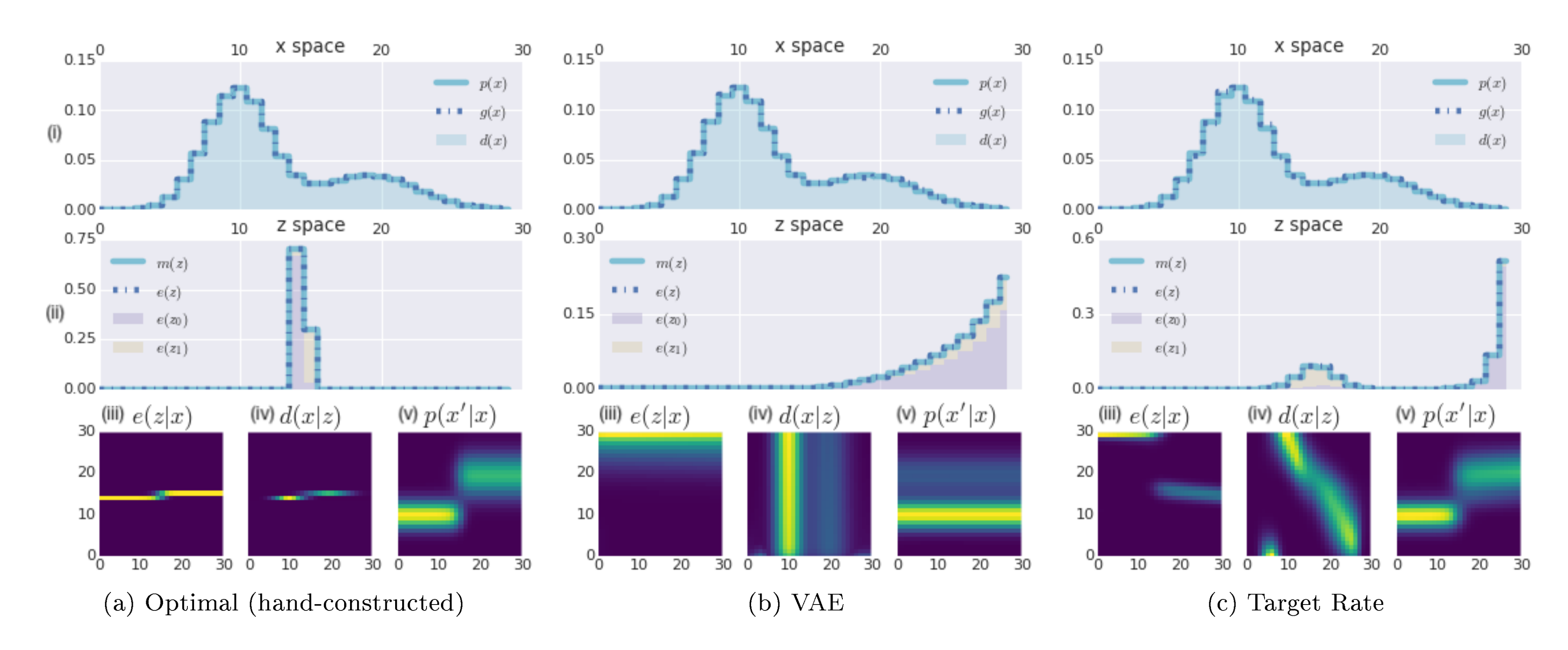
Figure 2 shows various distributions computed using three models. For the left column (Figure 2a), we use a hand-engineered encoder $e(z|x)$, decoder $d(x|z)$, and marginal $m(z)$ constructed with knowledge of the true data generating mechanism to illustrate an optimal model. For the middle (Figure 2b) and right (Figure 2c) columns, we learn $e(z|x)$, $d(x|z)$, and $m(z)$ using effectively infinite data sampled from $p^*(x)$ directly. The middle column (Figure 2b) is trained with ELBO. The right column (Figure 2c) is trained by targeting $R=0.5$ while minimizing $D$.[^2] In both cases, we see that $p^*(x) \approx g(x) \approx d(x)$ for both trained models (2bi, 2ci), indicating that optimization found the global optimum of the respective objectives. However, the VAE fails to learn a useful representation, only yielding a rate of $R=0.0002$ nats, [^3] while the Target Rate model achieves $R=0.4999$ nats. Additionally, it nearly perfectly reproduces the true generative process, as can be seen by comparing the yellow and purple regions in the z-space plots (2aii, 2cii) – both the optimal model and the Target Rate model have two clusters, one with about 70% of the probability mass, corresponding to class 0 (purple shaded region), and the other with about 30% of the mass (yellow shaded region) corresponding to class 1. In contrast, the z-space of the VAE (2bii) completely mixes the yellow and purple regions, only learning a single cluster. Note that we reproduced essentially identical results with dozens of different random initializations for both the VAE and the penalty VAE model – these results are not cherry-picked.

[^2]: Note that the target value $R = \operatorname{I}(x;z^*)=0.5$ is computed with knowledge of the true data generating distribution. However, this is the only information that is "leaked" to our method, and in general it is not hard to guess reasonable targets for $R$ for a given task and dataset.

[^3]: This is an example of VAEs ignoring the latent space. As decoder power increases, even $\beta=1$ is sufficient to cause the model to collapse to the autodecoding limit.

MNIST: $RD$ curve

In this section, we show how comparing models in terms of rate and distortion separately is more useful than simply observing marginal log likelihoods, and allows a detailed ablative comparison of individual architectural modifications. We use the static binary MNIST dataset from 31.

We examine several VAE model architectures that have been proposed in the literature. In particular, we consider simple and complex variants for the encoder and decoder, and three different types of marginal. The simple encoder is a CNN with a fully factored 64 dimensional Gaussian for $e(z|x)$; the more complex encoder is similar, but followed by 4 steps of mean-only Gaussian inverse autoregressive flow ([15]), with each step implemented as a 3 hidden layer MADE ([32]) with 640 units in each hidden layer. The simple decoder is a multilayer deconvolutional network; the more powerful decoder is a PixelCNN++ ([33]) model. The simple marginal is a fixed isotropic Gaussian, as is commonly used with VAEs; the more complicated version has a 4 step 3 layer MADE ([32]) mean-only Gaussian autoregressive flow ([16]). We also consider the setting in which the marginal uses the VampPrior from ([10]). We will denote the particular model combination by the tuple $(+/-, +/-, +/-/v)$, depending on whether we use a simple $(-)$ or complex $(+)$ (or $(v)$ VampPrior) version for the (encoder, decoder, marginal) respectively. In total we consider $2 \times 2 \times 3 = 12$ models. We train them all to minimize the $\beta$-VAE objective in Equation 4. Full details can be found in Appendix F. Runs were performed at various values of $\beta$ ranging from 0.1 to 10.0, both with and without KL annealing ([5]).

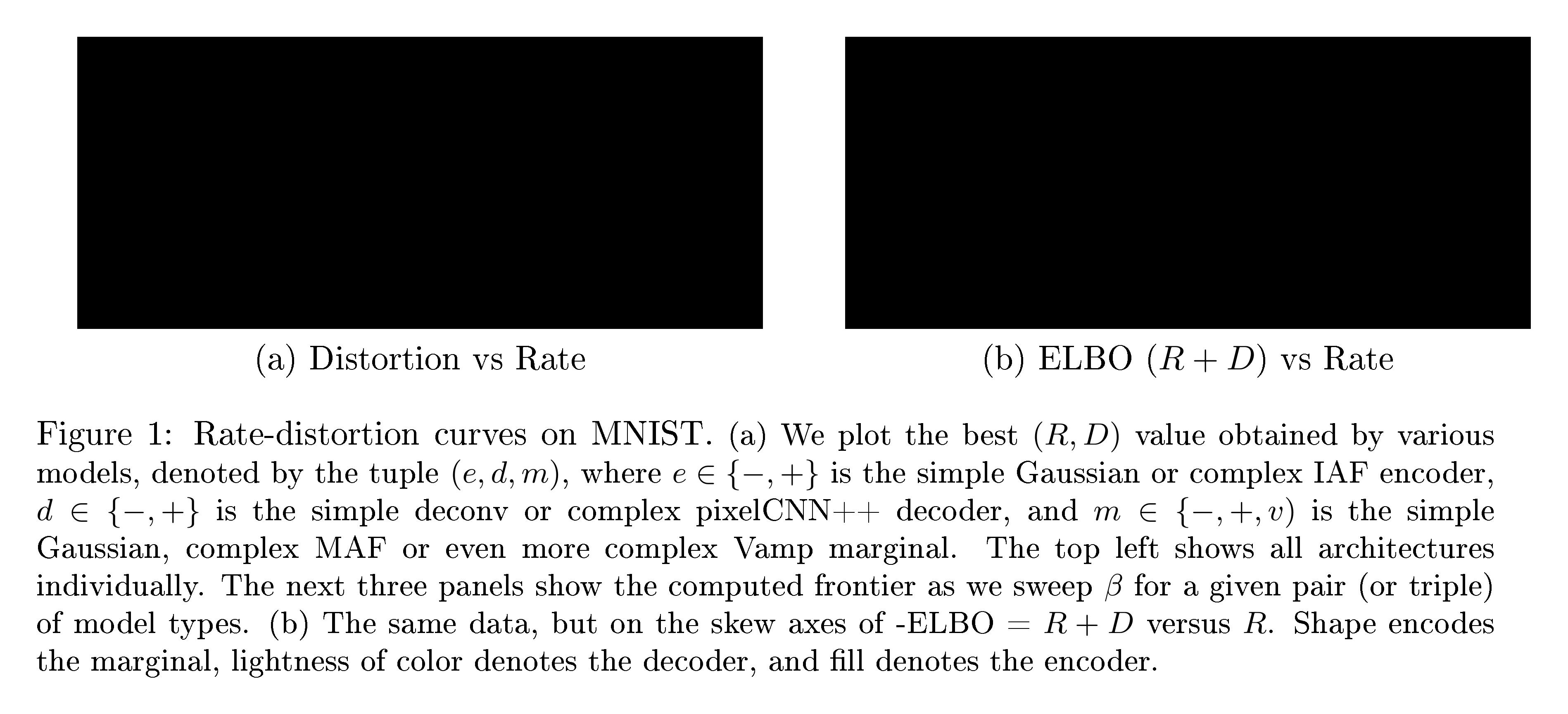
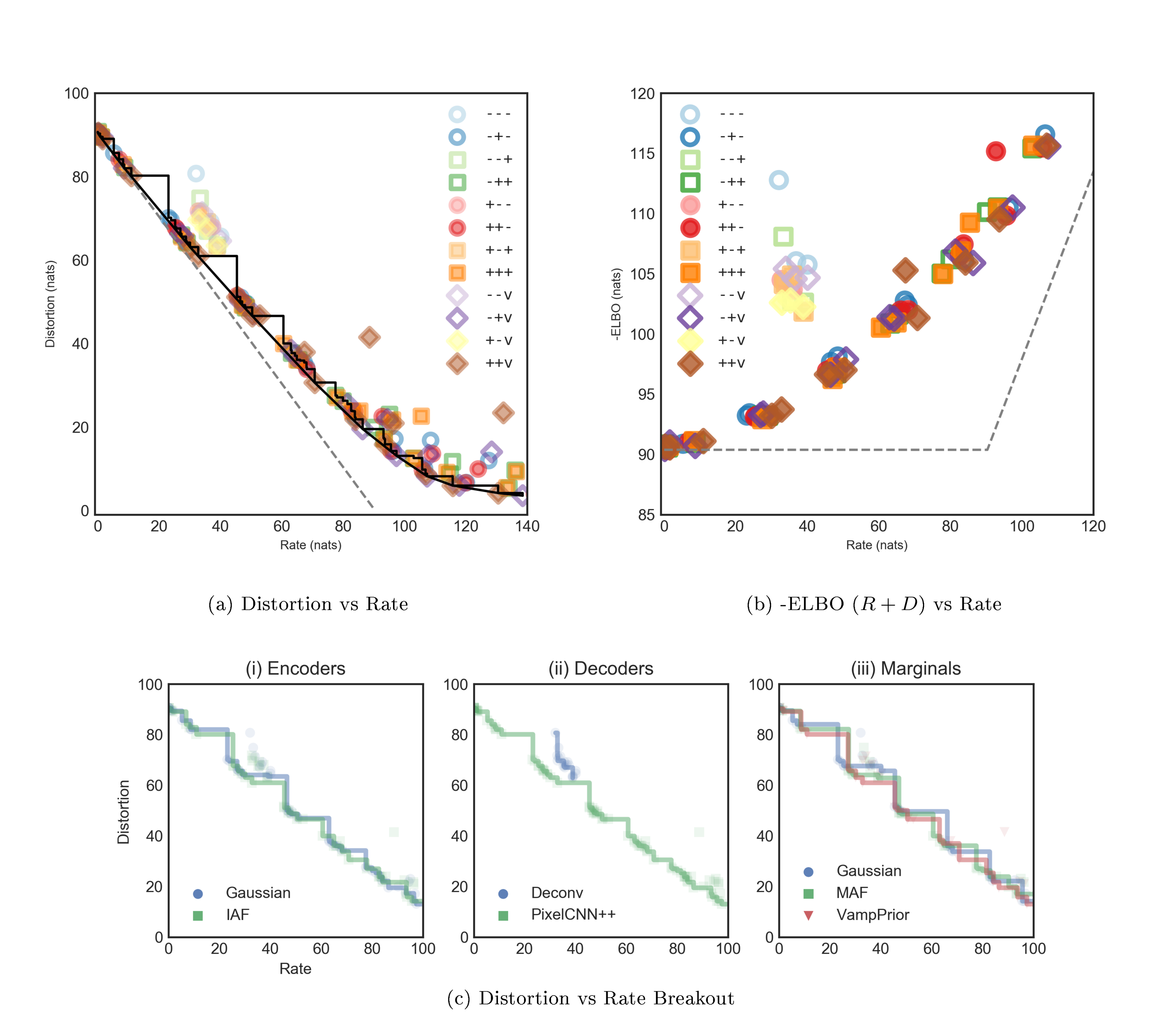
Figure 3a(i) shows the converged $RD$ location for a total of 209 distinct runs across our 12 architectures, with different initializations and $\beta$ s on the MNIST dataset. The best ELBO we achieved was $\hat{H} = 80.2$ nats, at $R=0$. This sets an upper bound on the true data entropy $H$ for the static MNIST dataset. The dashed line connects $(R=0, D=\hat{H})$ to $(R=\hat{H}, D=0)$, This implies that any $RD$ value above the dashed line is in principle achievable in a powerful enough model. The stepwise black curves show the monotonic Pareto frontier of achieved $RD$ points across all model families. The grey solid line shows the corresponding convex hull, which we approach closely across all rates. The 12 model families we considered here, arguably a representation of the classes of models considered in the VAE literature, in general perform much worse in the auto-encoding limit (bottom right corner) of the $RD$ plane. This is likely due to a lack of power in our current marginal approximations, and suggests more experiments with powerful autoregressive marginals, as in [34].

Figure 3a(iii) shows the same data, but this time focusing on the conservative Pareto frontier across all architectures with either a simple deconvolutional decoder (blue) or a complex autoregressive decoder (green). Notice the systematic failure of simple decoder models at the lowest rates. Besides that discrepancy, the frontiers largely track one another at rates above 22 nats. This is perhaps unsurprising considering we trained on the binary MNIST dataset, for which the measured pixel level sampling entropy on the test set is approximately 22 nats. When we plot the same data where we vary the encoder (ii) or marginal (iv) from simple to complex, we do not see any systematic trends. Figure 3b shows the same raw data, but we plot -ELBO= $R+D$ versus $R$. Here some of the differences between individual model families' performances are more easily resolved.

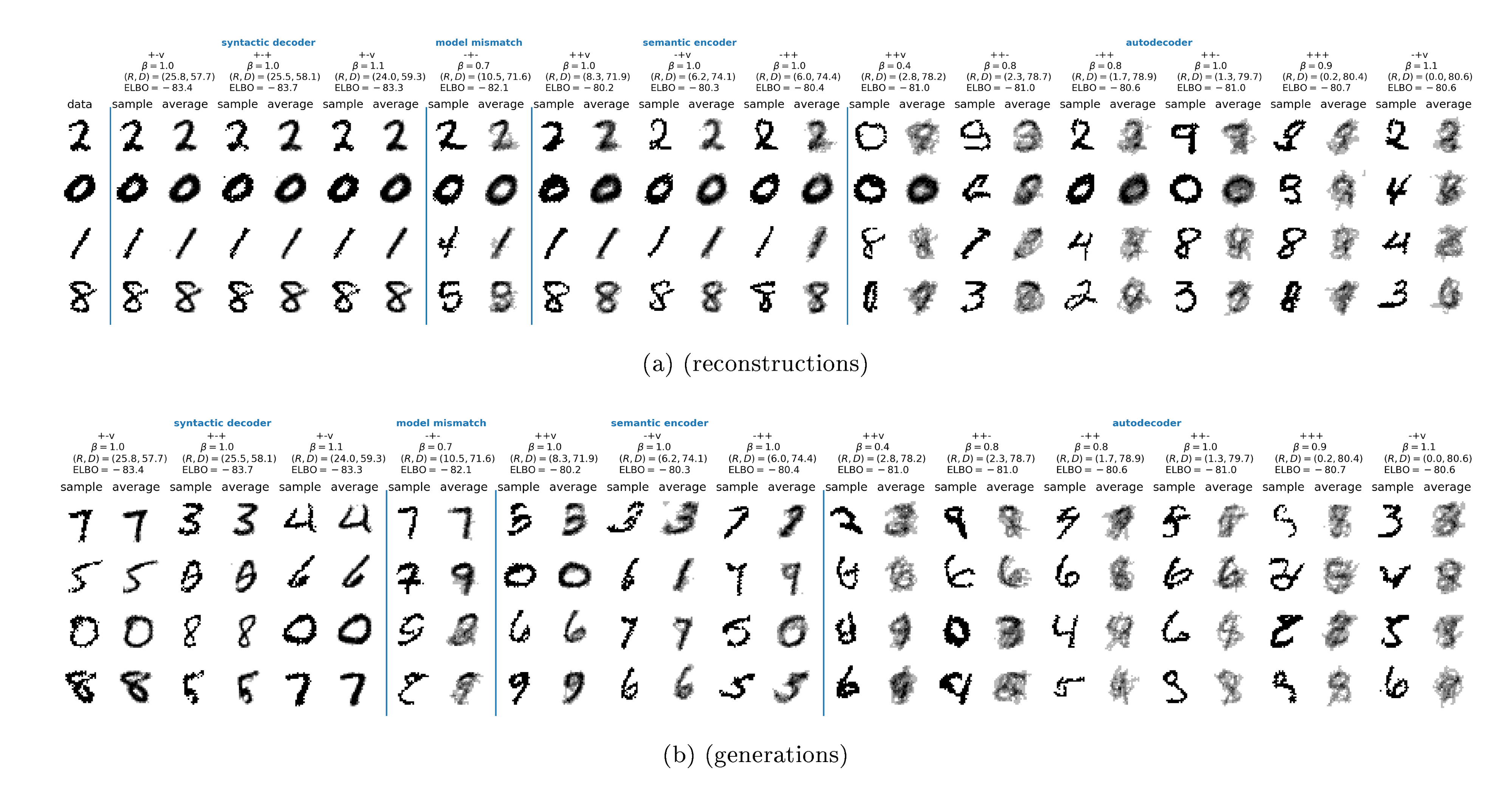
MNIST: Samples

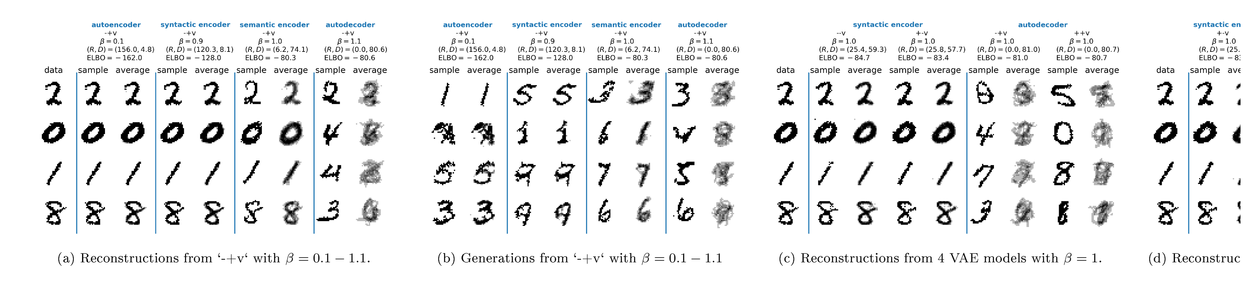
To qualitatively evaluate model performance, Figure 4 shows sampled reconstructions and generations from some of the runs, which we have grouped into rough categories: autoencoders, syntactic encoders, semantic encoders, and autodecoders. For reconstruction, we pick an image $x$ at random, encode it using $z \sim e(z|x)$, and then reconstruct it using $\hat{x} \sim d(x|z)$. For generation, we sample $z \sim m(z)$, and then decode it using $x \sim d(x|x)$. In both cases, we use the same $z$ each time we sample $x$, in order to illustrate the stochasticity implicit in the decoder. This is particularly important to do when using powerful decoders, such as autoregressive models.

In Figure 4a and Figure 4b, we study the effect of changing $\beta$ (using KL annealing from low to high) on the same -+v model, corresponding to a VAE with a simple encoder, a powerful PixelCNN++ decoder, and a powerful VampPrior marginal.

• When $\beta=1.10$ (right column), the model obtains $R = 0.0004$, $D=80.6$, ELBO=-80.6 nats, which is an example of an autodecoder. The tiny rate indicates that the decoder ignores its latent code, and hence the reconstructions are independent of the input $x$. For example, when the input is $x=8$ (bottom row), the reconstruction is $\hat{x}=3$. However, the generated images in Figure 4b sampled from the decoder look good. This is an example of an autodecoder.
• When $\beta=0.1$ (left column), the model obtains $R=156, D=4.8$, ELBO=-161 nats. Here the model is an excellent autoencoder, generating nearly pixel-perfect reconstructions. However, samples from this model's prior, as shown in Figure 4b, are very poor quality, which is also reflected in the worse ELBO. This is an example of an autoencoder.
• When $\beta = 1.0$, (third column), we get $R=6.2, D=74.1$, ELBO=-80.3. This model seems to retain semantically meaningful information about the input, such as its class and width of the strokes, but maintains syntactic variation in the individual reconstructions, so we call this a semantic encoder. In particular, notice that the input "2" is reconstructed as a similar "2" but with a visible loop at the bottom (top row). This model also has very good generated samples. This semantic encoding arguably typifies what we want to achieve in unsupervised learning: we have learned a highly compressed representation that retains semantic features of the data. We therefore call it a "semantic encoder".
• When $\beta=0.15$ (second column), we get $R=120.3, D=8.1$, ELBO=-128. This model retains both semantic and syntactic information, where each digit's style is maintained, and also has a good degree of compression. We call this a "syntactic encoder". However, at these higher rates the failures of our current architectures to approach their theoretical performance becomes more apparent, as the corresponding ELBO of 128 nats is much higher than the 81 nats we obtain at low rates. This is also evident in the visual degradation in the generated samples (Figure 4b).

Figure 4c shows what happens when we vary the model for a fixed value of $\beta=1$, as in traditional VAE training. Here only 4 architectures are shown (the full set is available in Figure 5 in the appendix), but the pattern is apparent: whenever we use a powerful decoder, the latent code is independent of the input, so it cannot reconstruct well. However, Figure 4a shows that by using $\beta < 1$, we can force such models to do well at reconstruction. Finally, Figure 4d shows 4 different models, chosen from the Pareto frontier, which all have almost identical ELBO scores, but which exhibit qualitatively different behavior.

Omniglot

We repeated the experiments on the omniglot dataset, and find qualitatively similar results. See Appendix B for details.

5. Discussion and further work

Section Summary: This paper introduces a new theoretical approach to representation learning in latent variable models, based on balancing data compression rates and reconstruction accuracy, which lets researchers target specific performance levels unlike older methods. Experiments on various VAE models reveal tradeoffs, such as the strength of autoregressive decoders at low compression rates, a tendency for advanced decoders to overlook the latent code (fixable by slightly reducing the regularization penalty), and the challenge of maintaining high compression with minimal errors, pointing to the need for improved approximations. The authors urge future studies to separately track compression and error rates rather than just overall likelihood scores to better compare model behaviors.

We have presented a theoretical framework for understanding representation learning using latent variable models in terms of the rate-distortion tradeoff. This constrained optimization problem allows us to fit models by targeting a specific point on the $RD$ curve, which we cannot do using the $\beta$-VAE framework.

In addition to the theoretical contribution, we have conducted a large set of experiments, which demonstrate the tradeoffs implicitly made by several recently proposed VAE models. We confirmed the power of autoregressive decoders, especially at low rates. We also confirmed that models with expressive decoders can ignore the latent code, and proposed a simple solution to this problem (namely reducing the KL penalty term to $\beta < 1$). This fix is much easier to implement than other solutions that have been proposed in the literature, and comes with a clear theoretical justification. Perhaps our most surprising finding is that all the current approaches seem to have a hard time achieving high rates at low distortion. This suggests the need to develop better marginal posterior approximations, which should in principle be able to reach the autoencoding limit, with vanishing distortion and rates approaching the data entropy.

Finally, we strongly encourage future work to report rate and distortion values independently, rather than just reporting the log likelihood, which fails to distinguish qualitatively different behavior of certain models.

Appendix

Section Summary: The appendix offers additional insights into variational autoencoders (VAEs) on datasets like static MNIST and Omniglot, showing how different model architectures balance information compression (rate) against reconstruction accuracy (distortion). On MNIST, it highlights a spectrum from autodecoders that produce noisy, low-info outputs to syntactic encoders capturing digit style and content, with some models failing to distinguish key image features. For Omniglot, powerful decoders dominate low-rate scenarios, and tuning a parameter called beta allows smooth shifts from pure generation to detailed encoding, while a final section explores mathematical bounds on mutual information in these generative processes.

Supplemental Materials: Fixing a Broken ELBO

A. More results on Static MNIST

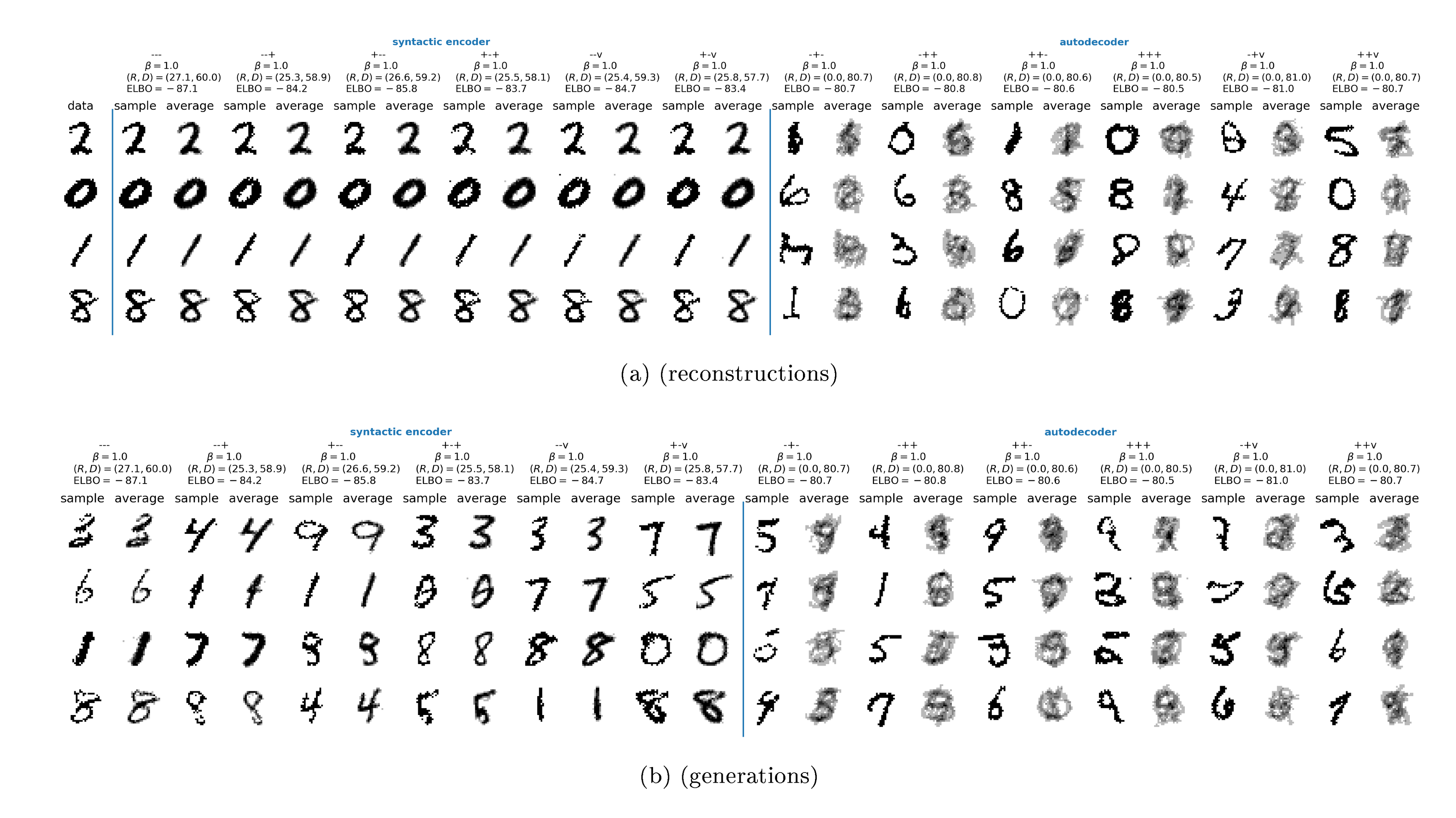
Figure 6 illustrates that many different architectures can participate in the optimal frontier and that we can achieve a smooth variation between the pure autodecoding models and models that encode more and more semantic and syntactic information. On the left, we see three syntactic encoders, which do a good job of capturing both the content of the digit and its style, while having variance in the decodings that seem to capture the sampling noise. On the right, we have six clear autodecoders, with very low rate and very high variance in the reconstructed or generated digit. In between are three semantic encoders, capturing the class of each digit, but showing a wide range of decoded style variation, which corresponds to the syntax of MNIST digits. Finally, between the syntactic encoders and semantic encoders lies a modeling failure, in which a weak encoder and marginal are paired with a strong decoder. The rate is sufficiently high for the decoder to reconstruct a good amount of the semantic and syntactic information, but it appears to have failed to learn to distinguish between the two.

B. Results on OMNIGLOT

Figure 7 plots the RD curve for various models fit to the Omniglot dataset ([35]), in the same form as the MNIST results in Figure 3. Here we explored $\beta$ s for the powerful decoder models ranging from 1.1 to 0.1, and $\beta$ s of 0.9, 1.0, and 1.1 for the weaker decoder models.

On Omniglot, the powerful decoder models dominate over the weaker decoder models. The powerful decoder models with their autoregressive form most naturally sit at very low rates. We were able to obtain finite rates by means of KL annealing. Our best achieved ELBO was at -90.37 nats, set by the ++- model with $\beta=1.0$ and KL annealing. This model obtains $R=0.77, D=89.60, ELBO=-90.37$ and is nearly auto-decoding. We found 14 models with ELBOs below 91.2 nats ranging in rates from 0.0074 nats to 10.92 nats.

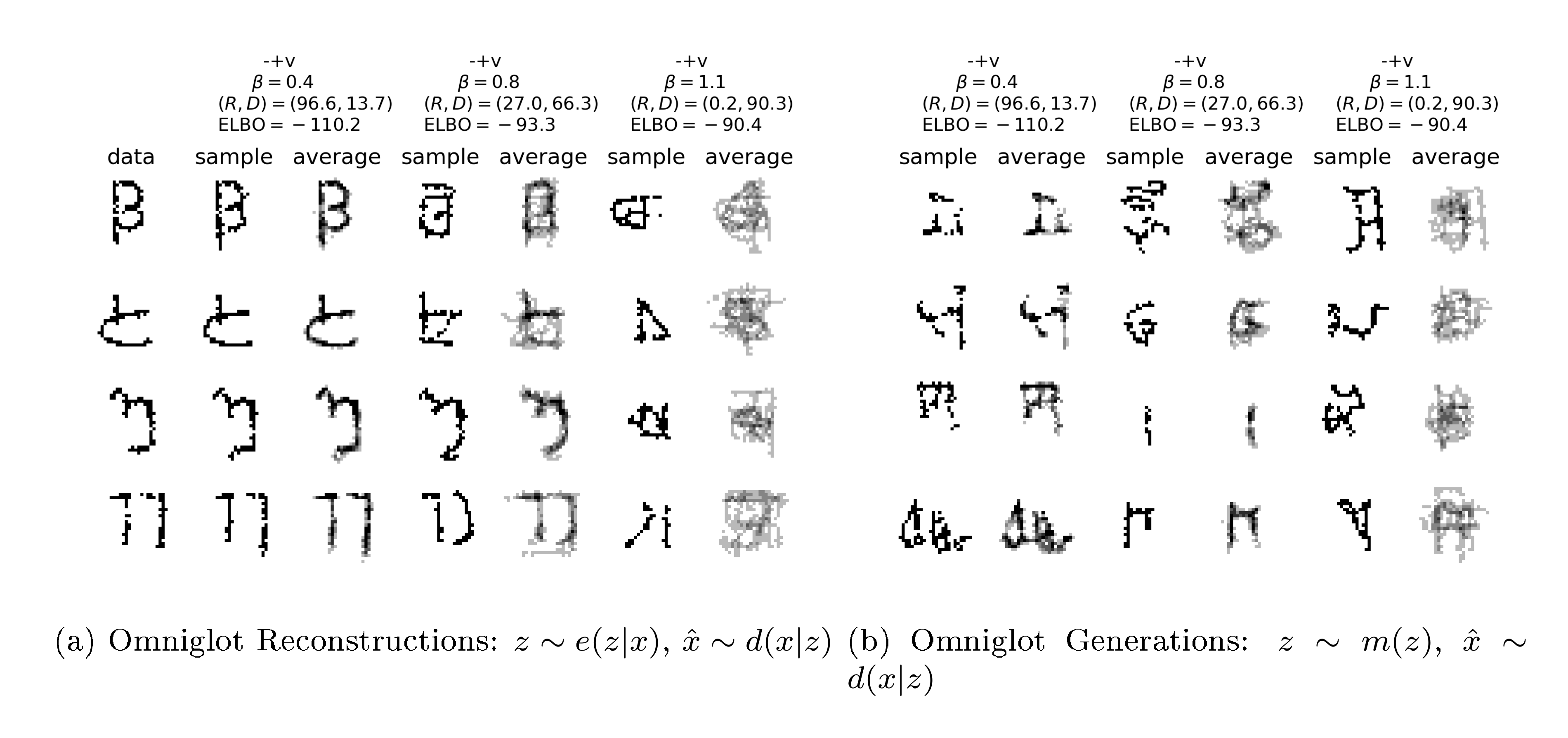
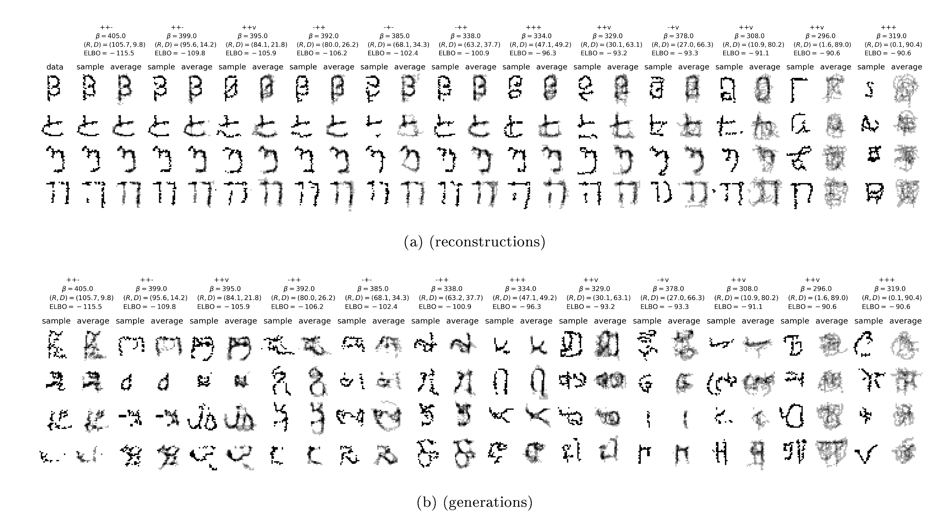
Similar to Figure 4 in Figure 8 we show sample reconstruction and generated images from the same "-+v" model family trained with KL annealing but at various $\beta$ s. Just like in the MNIST case, this demonstrates that we can smoothly interpolate between auto-decoding and auto-encoding behavior in a single model family, simply by adjusting the $\beta$ value.

C. Generative mutual information

Given any four distributions: $p^*(x)$ – a density over some data space $X$, $e(z|x)$ – a stochastic map from that data to a new representational space $Z$, $d(x|z)$ – a stochastic map in the reverse direction from $Z$ to $X$, and $m(z)$ – some density in the $Z$ space; we were able to find an inequality relating three functionals of these densities that must always hold. We found this inequality by deriving upper and lower bounds on the mutual information in the joint density defined by the natural representational path through the four distributions, $p_e(x, z) = p^*(x)e(z|x)$. Doing so naturally made us consider the existence of two other distributions $d(x|z)$ and $m(z)$. Let's consider the mutual information along this new generative path.

$ p_d(x, z) = m(z)d(x|z)\tag{5} $

$ \operatorname{I}_\mathrm{d}(X;Z) = \iint dx, dz, p_d(x, z) \log \frac{p_d(x, z)}{p_d(x)p_d(z)}\tag{6} $

Just as before we can easily establish both a variational lower and upper bound on this mutual information. For the lower bound (proved in Appendix D.5), we have:

$ E \equiv \int dz, p(z) \int dx, p(x|z) \log \frac{q(z|x)}{p(z)} \leq \operatorname{I}_\mathrm{d}\tag{7} $

Where we need to make a variational approximation to the decoder posterior, itself a distribution mapping $X$ to $Z$. Since we already have such a distribution from our other considerations, we can certainly use the encoding distribution $q(z|x)$ for this purpose, and since the bound holds for any choice it will hold with this choice. We will call this bound $E$ since it gives the distortion as measured through the encoder as it attempts to encode the generated samples back to their latent representation.

We can also find a variational upper bound on the generative mutual information (proved in Appendix D.6):

$ G \equiv \int dz, m(z) \int dx, d(x|z) \log \frac{d(x|z)}{q(x)} \geq \operatorname{I}_\mathrm{d}\tag{8} $

This time we need a variational approximation to the marginal density of our generative model, which we denote as $q(x)$. We call this bound $G$ for the rate in the generative model.

Together these establish both lower and upper bounds on the generative mutual information:

$ E \leq \operatorname{I}_\mathrm{d} \leq G.\tag{9} $

In our early experiments, it appears as though additionally constraining or targeting values for these generative mutual information bounds is important to ensure consistency in the underlying joint distributions. In particular, we notice a tendency of models trained with the $\beta$-VAE objective to have loose bounds on the generative mutual information when $\beta$ varies away from 1.

C.1. Rearranging the Representational Lower Bound

In light of the appearance of a new independent density estimate $q(x)$ in deriving our variational upper bound on the mutual information in the generative model, let's actually use that to rearrange our variational lower bound on the representational mutual information.

$ \int dx, p^*(x) \int dz, e(z|x) \log \frac{e(z|x)}{p^*(x)} = \int dx, p^*(x) \int dz, e(z|x) \log \frac{e(z|x)}{q(x)} - \int dx, p^*(x) \log \frac{p^*(x)}{q(x)}\tag{10} $

Doing this, we can express our lower bound in terms of two reparameterization independent functionals:

$ \begin{align} U &\equiv \int dx, p^*(x) \int dz, e(z|x) \log \frac{d(x|z)}{q(x)} \tag{a} \ S &\equiv \int dx, p^*(x) \log \frac{p^*(x)}{q(x)} = -\int dx, p^*(x) \log q(x) - H \tag{b} \end{align}\tag{11} $

This new reparameterization couples together the bounds we derived both the representational mutual information and the generative mutual information, using $q(x)$ in both. The new function $S$ we've described is intractable on its own, but when split into the data entropy and a cross entropy term, suggests we set a target cross entropy on our own density estimate $q(x)$ with respect to the empirical data distribution that might be finite in the case of finite data.

Together we have an equivalent way to formulate our original bounds on the representaional mutual information

$ U - S = H - D \leq I_{\text{rep}} \leq R\tag{12} $

We believe this reparameterization offers and important and potential way to directly control for overfitting. In particular, given that we compute our objectives using a finite sample from the true data distribution, it will generically be true that ${\operatorname{KL}!\left[\hat{p}(x) \mid\mid p^*(x) \right]} \geq 0$. In particular, the usual mode we operate in is one in which we only ever observe each example once in the training set, suggesting that in particular an estimate for this divergence would be:

$ {\operatorname{KL}!\left[\hat{p}(x) \mid\mid p^*(x) \right]} \sim H(X) - \log N. $

Early experiments suggest this offers a useful target for $S$ in the reparameterized objective that can prevent overfitting, at least in our toy problems.

D. Proofs

D.1. Lower Bound on Representational Mutual Information

Our lower bound is established by the fact that Kullback-Leibler (KL) divergences are positive semidefinite

$

{\operatorname{KL}\!\left[q(x|z) \mid\mid p(x|z) \right]} = \int dx\, q(x|z) \log \frac{q(x|z)}{p(x|z)} \geq 0

$

which implies for any distribution $p(x|z)$:

$ \int dx, q(x|z) \log q(x|z) \geq \int dx, q(x|z) \log p(x|z) $

$ \begin{align*} \operatorname{I}\mathrm{e} &= \operatorname{I}\mathrm{e}(X; Z) = \iint dx, dz, p_e(x, z) \log \frac{p_e(x, z)}{p^*(x)p_e(z)} \ &= \int dz, p_e(z) \int dx, p_e(x|z) \log \frac{p_e(x|z)}{p^*(x)} \ &= \int dz, p_e(z) \left[\int dx, p_e(x|z) \log p_e(x|z) - \int dx, p_e(x|z) \log p^*(x) \right] \ &\geq \int dz, p_e(z) \left[\int dx, p_e(x|z) \log d(x|z) - \int dx, p_e(x|z) \log p^*(x) \right] \ &= \iint dx, dz, p_e(x, z) \log \frac{d(x|z)}{p^*(x)} \ &= \int dx, p^*(x) \int dz, e(z|x) \log \frac{d(x|z)}{p^*(x)} \ &= \left(-\int dx, p^*(x) \log p^*(x)\right) - \left(-\int dx, p^*(x) \int dz, e(z|x) \log d(x|z)\right) \ &\equiv H - D \end{align*} $

D.2. Upper Bound on Representational Mutual Information

The upper bound is established again by the positive semidefinite quality of KL divergence.

$

{\operatorname{KL}\!\left[q(z|x) \mid\mid p(z) \right]} \geq 0 \implies \int dz\, q(z|x) \log q(z|x) \geq \int dz\, q(z|x) \log p(z)

$

$ \begin{align*} \operatorname{I}\mathrm{e} &= \operatorname{I}\mathrm{e}(X; Z) = \iint dx, dz, p_e(x, z) \log \frac{p_e(x, z)}{p^*(x)p_e(z)} \ &= \iint dx, dz, p_e(x, z) \log \frac{e(z|x)}{p_e(z)} \ &= \iint dx, dz, p_e(x, z) \log e(z|x) - \iint dx, dz, p_e(x, z) \log p_e(z) \ &= \iint dx, dz, p_e(x, z) \log e(z|x) - \int dz, p_e(z) \log p_e(z) \ &\leq \iint dx, dz, p_e(x, z) \log e(z|x) - \int dz, p_e(z) \log m(z) \ &= \iint dx, dz, p_e(x, z) \log e(z|x) - \iint dx, dz, p_e(x, z) \log m(z) \ &= \iint dx, dz, p_e(x, z) \log \frac{e(z|x)}{m(z)} \ &= \int dx, p^*(x) \int dz, e(z|x) \log \frac{e(z|x)}{m(z)} \equiv R \end{align*} $

D.3. Optimal Marginal for Fixed Encoder

Here we establish that the optimal marginal approximation $p(z)$, is precisely the marginal distribution of the encoder.

$ R \equiv \int dx, p^*(x) \int dz, e(z|x) \log \frac{e(z|x)}{m(z)} $

Consider the variational derivative of the rate with respect to the marginal approximation:

$ m(z) \to m(z) + \delta m(z) \quad \int dz, \delta m(z) = 0 $

$ \begin{align*} \delta R &= \int dx, p^*(x) \int dz, e(z|x) \log \frac{e(z|x)}{m(z) + \delta m(z)} - R \ &= \int dx, p^*(x) \int dz, e(z|x) \log \left(1 + \frac{\delta m(z)}{m(z)} \right) \ &\sim \int dx, p^*(x) \int dz, e(z|x) \frac{\delta m(z)}{m(z)} \end{align*} $

Where in the last line we have taken the first order variation, which must vanish if the total variation is to vanish. In particular, in order for this variation to vanish, since we are considering an arbitrary $\delta m(z)$, except for the fact that the integral of this variation must vanish, in order for the first order variation in the rate to vanish it must be true that for every value of $x, z$ we have that:

$ m(z) \propto p^*(x) e(z|x), $

which when normalized gives:

$ m(z) = \int dx, p^*(x) e(z|x), $

or that the marginal approximation is the true encoder marginal.

D.4. Optimal Decoder for Fixed Encoder

Next consider the variation in the distortion in terms of the decoding distribution with a fixed encoding distribution.

$ d(x|z) \to d(x|z) + \delta d(x|z) \quad \int dx, d(x|z) = 0 $

$ \begin{align*} \delta D &= -\int dx, p^*(x) \int dz, e(z|x) \log (d(x|z) + \delta d(x|z)) - D\ &= -\int dx, p^*(x) \int dz, e(z|x) \log \left(1 + \frac{\delta d(x|z)}{d(x|z)} \right) \ &\sim -\int dx, p^*(x) \int dz, e(z|x) \frac{\delta d(x|z)}{d(x|z)} \end{align*} $

Similar to the section above, we took only the leading variation into account, which itself must vanish for the full variation to vanish. Since our variation in the decoder must integrate to 0, this term will vanish for every $x, z$ we have that:

$ d(x|z) \propto p^*(x) e(z|x), $

when normalized this gives:

$ d(x|z) = e(z|x) \frac{p^*(x)}{\int dx, p^*(x) e(z|x)} $

which ensures that our decoding distribution is the correct posterior induced by our data and encoder.

D.5. Lower bound on Generative Mutual Information

The lower bound is established as all other bounds have been established, with the positive semidefiniteness of KL divergences.

$

{\operatorname{KL}\!\left[d(z|x) \mid\mid q(z|x) \right]} = \int dz\, d(z|x) \log \frac{d(z|x)}{q(z|x)} \geq 0

$

which implies for any distribution $q(z|x)$:

$ \int dz, d(z|x) \log d(z|x) \geq \int dz, d(z|x) \log q(z|x) $

$ \begin{align*} I_{\text{gen}} &= I_{\text{gen}}(X; Z) = \iint dx, dz, p_d(x, z) \log \frac{p_d(x, z)}{p_d(x)p_d(z)} \ &= \int dx, p_d(x) \int dz, p_d(z|x) \log \frac{p_d(z|x)}{m(z)} \ &= \int dx, p_d(x) \left[\int dz, p_d(z|x) \log p_d(z|x) - \int dz, p_d(z|x) \log m(z) \right] \ &\geq \int dx, p_d(x) \left[\int dz, p_d(z|x) \log e(z|x) - \int dz, p_d(z|x) \log m(z) \right] \ &= \iint dx, dz, p_d(x, z) \log \frac{e(z|x)}{m(z)} \ &= \int dz, m(z) \int dx, d(x|z) \log \frac{e(z|x)}{m(z)} \ &\equiv E \end{align*} $

D.6. Upper Bound on Generative Mutual Information

The upper bound is establish again by the positive semidefinite quality of KL divergence.

$

{\operatorname{KL}\!\left[p(x|z) \mid\mid r(x) \right]} \geq 0 \implies \int dx\, p(x|z) \log p(x|z) \geq \int dx\, p(x|z) \log r(x)

$

$ \begin{align*} I_{\text{gen}} &= I_{\text{gen}}(X; Z) = \iint dx, dz, p_d(x, z) \log \frac{p_d(x, z)}{p_d(x)m(z)} \ &= \iint dx, dz, p_d(x, z) \log \frac{d(x|z)}{p_d(x)} \ &= \iint dx, dz, p_d(x, z) \log d(x|z) - \iint dx, dz, p_d(x, z) \log p_d(x) \ &= \iint dx, dz, p_d(x, z) \log d(x|z) - \int dx, p_d(x) \log p_d(x) \ &\leq \iint dx, dz, p_d(x, z) \log d(x|z) - \int dx, p_d(x) \log q(x) \ &= \iint dx, dz, p_d(x, z) \log d(x|z) - \iint dx, dz, p_d(x, z) \log q(x) \ &= \iint dx, dz, p_d(x, z) \log \frac{d(x|z)}{q(x)} \ &= \int dz, m(z) \int dx, d(x|z) \log \frac{d(x|z)}{q(x)} \equiv G \end{align*} $

E. Toy Model Details

Data generation.

The true data generating distribution is as follows. We first sample a latent binary variable, $z \sim \mathrm{Ber}(0.7)$, then sample a latent 1d continuous value from that variable, $h|z \sim \mathcal{N}(h|\mu_z, \sigma_z)$, and finally we observe a discretized value, $x = \mathrm{discretize}(h; \mathcal{B})$, where $\mathcal{B}$ is a set of 30 equally spaced bins. We set $\mu_z$ and $\sigma_z$ such that $R^* \equiv \operatorname{I}(x;z)=0.5$ nats, in the true generative process, representing the ideal rate target for a latent variable model.

Model details.

We choose to use a discrete latent representation with $K=30$ values, with an encoder of the form $e(z_i|x_j) \propto -\exp[(w^e_i x_j - b^e_i)^2]$, where $z$ is the one-hot encoding of the latent categorical variable, and $x$ is the one-hot encoding of the observed categorical variable. Thus the encoder has $2K=60$ parameters. We use a decoder of the same form, but with different parameters: $d(x_j|z_i) \propto -\exp[(w^d_i x_j - b^d_i)^2]$. Finally, we use a variational marginal, $m(z_i)=\pi_i$. Given this, the true joint distribution has the form $p_e(x, z) = p^*(x) e(z|x)$, with marginal $m(z) = \sum_x p_e(x, z)$ and conditional $p_e(x|z) = p_e(x, z)/ p_e(z)$.

F. Details for MNIST and Omniglot Experiments

We used the static binary MNIST dataset originally produced for (Larochelle & Murray, 2011)^5, and the Omniglot dataset from Lake et al. (2015); Burda et al. (2015).

As stated in the main text, for our experiments we considered twelve different model families corresponding to a simple and complex choice for the encoder and decoder and three different choices for the marginal.

Unless otherwise specified, all layers used a linearly gated activation function activation function (Dauphin et al., 2017), $h(x) = (W_1 x + b_2) \sigma(W_2 x + b_2)$.

F.1. Encoder architectures

For the encoder, the simple encoder was a convolutional encoder outputting parameters to a diagonal Gaussian distribution. The inputs were first transformed to be between -1 and 1. The architecture contained 5 convolutional layers, summarized in the format Conv (depth, kernel size, stride, padding), followed by a linear layer to read out the mean and a linear layer with softplus nonlinearity to read out the variance of the diagonal Gaussiann distribution.

• Input (28, 28, 1)
• Conv (32, 5, 1, same)
• Conv (32, 5, 2, same)
• Conv (64, 5, 1, same)
• Conv (64, 5, 2, same)
• Conv (256, 7, 1, valid)
• Gauss (Linear (64), Softplus (Linear (64)))

For the more complicated encoder, the same 5 convolutional layer architecture was used, followed by 4 steps of mean-only Gaussian inverse autoregressive flow, with each step's location parameters computed using a 3 layer MADE style masked network with 640 units in the hidden layers and ReLU activations.

F.2. Decoder architectures

The simple decoder was a transposed convolutional network, with 6 layers of transposed convolution, denoted as Deconv (depth, kernel size, stride, padding) followed by a linear convolutional layer parameterizing an independent Bernoulli distribution over all of the pixels:

• Input (1, 1, 64)
• Deconv (64, 7, 1, valid)
• Deconv (64, 5, 1, same)
• Deconv (64, 5, 2, same)
• Deconv (32, 5, 1, same)
• Deconv (32, 5, 2, same)
• Deconv (32, 4, 1, same)
• Bernoulli (Linear Conv (1, 5, 1, same))

The complicated decoder was a slightly modified PixelCNN++ style network (Salimans et al., 2017)[^6]. However in place of the original RELU activation functions we used linearly gated activation functions and used six blocks (with sizes $(28\times 28)$ – $(14\times 14)$ – $(7\times 7)$ – $(7\times 7)$ – $(14\times 14)$ – $(28\times 28)$) of two resnet layers in each block. All internal layers had a feature depth of 64. Shortcut connections were used throughout between matching sized featured maps. The 64-dimensional latent representation was sent through a dense lineary gated layer to produce a 784-dimensional representation that was reshaped to $(28\times 28\times 1)$ and concatenated with the target image to produce a $(28\times 28\times 2)$ dimensional input. The final output (of size $(28\times28\times64)$) was sent through a $(1\times 1)$ convolution down to depth 1. These were interpreted as the logits for a Bernoulli distribution defined on each pixel.

[^6]: Original implmentation available at https://github.com/openai/pixel-cnn

F.3. Marginal architectures

We used three different types of marginals. The simplest architecture (denoted (-)), was just a fixed isotropic gaussian distribution in 64 dimensions with means fixed at 0 and variance fixed at 1.

The complicated marginal (+) was created by transforming the isotropic Gaussian base distribution with 4 layers of mean-only Gaussian autoregressive flow, with each steps location parameters computed using a 3 layer MADE style masked network with 640 units in the hidden layers and relu activations. This network resembles the architecture used in Papamakarios et al. (2017).

The last choice of marginal was based on VampPrior and denoted with (v), which uses a mixture of the encoder distributions computed on a set of pseudo-inputs to parameterize the prior (Tomczak & Welling, 2017). We add an additional learned set of weights on the mixture distributions that are constrained to sum to one using a softmax function: $m(z) =\sum_{i=1}^N w_i e(z|\phi_i)$ where $N$ are the number of pseudo-inputs, $w$ are the weights, $e$ is the encoder, and $\phi$ are the pseudo-inputs that have the same dimensionality as the inputs.

F.4. Optimization

The models were all trained using the $\beta$-VAE objective (Higgins et al., 2017) at various values of $\beta$. No form of explicit regularization was used. The models were trained with Adam (Kingma & Ba, 2015) with normalized gradients (Yu et al., 2017) for 200 epochs to get good convergence on the training set, with a fixed learning rate of $3 \times 10^{-4}$ for the first 100 epochs and a linearly decreasing learning rate towards 0 at the 200th epoch.

References

Section Summary: This section lists key academic references on advanced topics in machine learning and artificial intelligence, including seminal papers on variational autoencoders, which are models that help computers learn and generate data representations efficiently. It covers foundational works from the 1990s to 2018, exploring ideas like information maximization, probabilistic inference, and generative networks, often published in top conferences such as ICLR, ICML, and NeurIPS. The citations draw from researchers like Kingma, Welling, and Tishby, providing building blocks for techniques in image compression, representation learning, and deep generative models.

[1] Kingma, Diederik P and Welling, Max. Auto-encoding variational Bayes. In ICLR, 2014.

[2] Rezende, Danilo Jimenez, Mohamed, Shakir, and Wierstra, Daan. Stochastic backpropagation and approximate inference in deep generative models. In ICML, 2014.

[3] Huszár, Ferenc. Is maximum likelihood useful for representation learning?, 2017. URL http://www.inference.vc/maximum-likelihood-for-representation-learning-2/.

[4] Phuong, Mary, Welling, Max, Kushman, Nate, Tomioka, Ryota, and Nowozin, Sebastian. The mutual autoencoder: Controlling information in latent code representations, 2018. URL https://openreview.net/forum?id=HkbmWqxCZ.

[5] Bowman, Samuel R, Vilnis, Luke, Vinyals, Oriol, Dai, Andrew M, Jozefowicz, Rafal, and Bengio, Samy. Generating sentences from a continuous space. CoNLL, 2016.

[6] Chen, X., Kingma, D. P., Salimans, T., Duan, Y., Dhariwal, P., Schulman, J., Sutskever, I., and Abbeel, P. Variational Lossy Autoencoder. In ICLR, 2017.

[7] Higgins, Irina, Matthey, Loic, Pal, Arka, Burgess, Christopher, Glorot, Xavier, Botvinick, Matthew, Mohamed, Shakir, and Lerchner, Alexander. $\beta$-VAE: Learning Basic Visual Concepts with a Constrained Variational Framework. In ICLR, 2017.

[8] Alemi, Alexander A, Fischer, Ian, Dillon, Joshua V, and Murphy, Kevin. Deep Variational Information Bottleneck. In ICLR, 2017.

[9] Makhzani, Alireza, Shlens, Jonathon, Jaitly, Navdeep, and Goodfellow, Ian. Adversarial autoencoders. In ICLR, 2016.

[10] Tomczak, J. M. and Welling, M. VAE with a VampPrior. ArXiv e-prints, 2017.

[11] Barber, David and Agakov, Felix V. Information maximization in noisy channels : A variational approach. In NIPS. 2003.

[12] Agakov, Felix Vsevolodovich. Variational Information Maximization in Stochastic Environments. PhD thesis, University of Edinburgh, 2006.

[13] Ha, David and Eck, Doug. A neural representation of sketch drawings. International Conference on Learning Representations, 2018. URL https://openreview.net/forum?id=Hy6GHpkCW.

[14] Hinton, Geoffrey E and Van Camp, Drew. Keeping the neural networks simple by minimizing the description length of the weights. In Proc. of the Workshop on Computational Learning Theory, 1993.

[15] Kingma, Diederik P, Salimans, Tim, Jozefowicz, Rafal, Chen, Xi, Sutskever, Ilya, and Welling, Max. Improved variational inference with inverse autoregressive flow. In NIPS. 2016.

[16] Papamakarios, George, Murray, Iain, and Pavlakou, Theo. Masked autoregressive flow for density estimation. In NIPS. 2017.

[17] Tishby, N., Pereira, F.C., and Biale, W. The information bottleneck method. In The 37th annual Allerton Conf. on Communication, Control, and Computing, pp.\ 368–377, 1999. URL https://arxiv.org/abs/physics/0004057.

[18] Shamir, Ohad, Sabato, Sivan, and Tishby, Naftali. Learning and generalization with the information bottleneck. Theoretical Computer Science, 411(29):2696 – 2711, 2010.

[19] Tishby, N. and Zaslavsky, N. Deep learning and the information bottleneck principle. In 2015 IEEE Information Theory Workshop (ITW), 2015.

[20] Achille, A. and Soatto, S. Information Dropout: Learning Optimal Representations Through Noisy Computation. In Information Control and Learning, September 2016. URL http://arxiv.org/abs/1611.01353.

[21] Achille, A. and Soatto, S. Emergence of Invariance and Disentangling in Deep Representations. Proceedings of the ICML Workshop on Principled Approaches to Deep Learning, 2017.

[22] Bell, Anthony J and Sejnowski, Terrence J. An information-maximization approach to blind separation and blind deconvolution. Neural computation, 7(6):1129–1159, 1995.

[23] Slonim, Noam, Atwal, Gurinder Singh, Tkačik, Gašper, and Bialek, William. Information-based clustering. PNAS, 102(51):18297–18302, 2005.

[24] Hoffman, Matthew D and Johnson, Matthew J. Elbo surgery: yet another way to carve up the variational evidence lower bound. In NIPS Workshop in Advances in Approximate Bayesian Inference, 2016.

[25] Zhao, Shengjia, Song, Jiaming, and Ermon, Stefano. The information-autoencoding family: A lagrangian perspective on latent variable generative modeling, 2018. URL https://openreview.net/forum?id=ryZERzWCZ.

[26] Zhao, Shengjia, Song, Jiaming, and Ermon, Stefano. Infovae: Information maximizing variational autoencoders. arXiv preprint 1706.02262, 2017.

[27] Chen, Xi, Duan, Yan, Houthooft, Rein, Schulman, John, Sutskever, Ilya, and Abbeel, Pieter. Infogan: Interpretable representation learning by information maximizing generative adversarial nets. arXiv preprint 1606.03657, 2016.

[28] Gregor, Karol, Besse, Frederic, Rezende, Danilo Jimenez, Danihelka, Ivo, and Wierstra, Daan. Towards conceptual compression. In Advances In Neural Information Processing Systems, pp.\ 3549–3557, 2016.

[29] Ballé, J., Laparra, V., and Simoncelli, E. P. End-to-end Optimized Image Compression. In ICLR, 2017.

[30] Johnston, N., Vincent, D., Minnen, D., Covell, M., Singh, S., Chinen, T., Hwang, S. J., Shor, J., and Toderici, G. Improved Lossy Image Compression with Priming and Spatially Adaptive Bit Rates for Recurrent Networks. ArXiv e-prints, 2017.

[31] Larochelle, Hugo and Murray, Iain. The neural autoregressive distribution estimator. In AI/Statistics, 2011.

[32] Germain, Mathieu, Gregor, Karol, Murray, Iain, and Larochelle, Hugo. Made: Masked autoencoder for distribution estimation. In ICML, 2015.

[33] Salimans, Tim, Karpathy, Andrej, Chen, Xi, and Kingma, Diederik P. Pixelcnn++: Improving the pixelcnn with discretized logistic mixture likelihood and other modifications. In ICLR, 2017.

[34] van den Oord, Aaron, Vinyals, Oriol, and kavukcuoglu, koray. Neural discrete representation learning. In NIPS. 2017.

[35] Lake, Brenden M., Salakhutdinov, Ruslan, and Tenenbaum, Joshua B. Human-level concept learning through probabilistic program induction. Science, 350(6266):1332–1338, 2015.