Deep Neural Networks for YouTube Recommendations

Paul Covington, Jay Adams, Emre Sargin
Google
Mountain View, CA
{pcovington, jka, msargin}@google.com

Abstract

YouTube represents one of the largest scale and most sophisticated industrial recommendation systems in existence. In this paper, we describe the system at a high level and focus on the dramatic performance improvements brought by deep learning. The paper is split according to the classic two-stage information retrieval dichotomy: first, we detail a deep candidate generation model and then describe a separate deep ranking model. We also provide practical lessons and insights derived from designing, iterating and maintaining a massive recommendation system with enormous user-facing impact.

Executive Summary: YouTube faces a massive recommendation challenge: serving personalized videos to over a billion users from a corpus that grows by many hours of new content every second. The prior matrix-factorization system could not keep pace with scale, rapidly changing popularity, and noisy implicit feedback such as watches rather than explicit ratings.

This paper therefore set out to replace that system with deep neural networks that perform the two classic stages of retrieval—candidate generation and ranking—while directly optimizing live user-engagement metrics.

The authors trained two separate feed-forward networks on hundreds of billions of examples. The first network embeds a user’s recent watches and searches, adds demographic and freshness signals, and learns to classify the next video the user will watch. The second network scores a few hundred candidates with hundreds of additional features and is trained to predict expected watch time rather than simple click probability. Both models were evaluated on hold-out data and, crucially, through live A/B experiments that measured watch time and other engagement signals.

The deepest networks (three hidden layers of 1 024, 512, and 256 rectified units) reduced weighted pairwise ranking loss by roughly 17 % relative to a linear baseline and produced the best accuracy within serving-cost limits. Adding an “example-age” feature removed the model’s bias toward older videos and increased watch time on recently uploaded content in live tests. Predicting the user’s next watch, rather than a random past watch, better captured asymmetric consumption patterns and lifted live metrics. Ranking by predicted watch time, instead of click-through rate, sharply reduced exposure of click-bait videos.

These gains matter because recommendations drive the majority of YouTube watch time. Even modest lifts in precision and freshness translate into billions of additional hours viewed and materially affect both user satisfaction and revenue.

The work demonstrates that deep networks, properly supplied with temporal and behavioral features, now outperform the previous generation of linear and tree-based methods at industrial scale. Teams maintaining similar systems should therefore migrate candidate generation and ranking to deep architectures, adopt watch-time-weighted objectives, and treat example age as a first-class input. Further gains are likely from richer sequence modeling and continued live experimentation.

The main limitations are that final claims rest on A/B tests whose results can shift with product changes, and that the reported improvements are tied to YouTube’s particular data distribution and serving constraints. Within those bounds the evidence is strong and directly actionable.

Keywords

recommender system; deep learning; scalability

1. INTRODUCTION

Section Summary: YouTube relies on deep learning to power its massive video recommendation system, which helps a billion users discover personalized content from an enormous and rapidly growing collection of videos. The approach tackles key difficulties such as operating at enormous scale, quickly adapting to new uploads and user actions, and handling unpredictable or messy user behavior data, all enabled by flexible tools like TensorFlow for training billion-parameter models. The paper outlines how these neural networks improve both the selection of candidate videos and the ranking of results by predicted watch time, contrasting with older matrix factorization techniques.

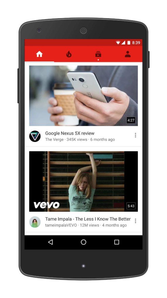
YouTube is the world’s largest platform for creating, sharing and discovering video content. YouTube recommendations are responsible for helping more than a billion users discover personalized content from an ever-growing corpus of videos. In this paper we will focus on the immense impact deep learning has recently had on the YouTube video recommendations system. Figure 1 illustrates the recommendations on the YouTube mobile app home.

Recommending YouTube videos is extremely challenging from three major perspectives:

• Scale: Many existing recommendation algorithms proven to work well on small problems fail to operate on our scale. Highly specialized distributed learning algorithms and efficient serving systems are essential for handling YouTube’s massive user base and corpus.
• Freshness: YouTube has a very dynamic corpus with many hours of video are uploaded per second. The recommendation system should be responsive enough to model newly uploaded content as well as the latest actions taken by the user. Balancing new content with well-established videos can be understood from an exploration/exploitation perspective.
• Noise: Historical user behavior on YouTube is inherently difficult to predict due to sparsity and a variety of unobservable external factors. We rarely obtain the ground truth of user satisfaction and instead model noisy implicit feedback signals. Furthermore, metadata associated with content is poorly structured without a well defined ontology. Our algorithms need to be robust to these particular characteristics of our training data.

In conjugation with other product areas across Google, YouTube has undergone a fundamental paradigm shift towards using deep learning as a general-purpose solution for nearly all learning problems. Our system is built on Google Brain [4] which was recently open sourced as TensorFlow [1]. TensorFlow provides a flexible framework for experimenting with various deep neural network architectures using large-scale distributed training. Our models learn approximately one billion parameters and are trained on hundreds of billions of examples.

In contrast to vast amount of research in matrix factorization methods [19], there is relatively little work using deep neural networks for recommendation systems. Neural networks are used for recommending news in [17], citations in [8] and review ratings in [20]. Collaborative filtering is formulated as a deep neural network in [22] and autoencoders in [18]. Elkahky et al. used deep learning for cross domain user modeling [5]. In a content-based setting, Burges et al. used deep neural networks for music recommendation [21].

The paper is organized as follows: A brief system overview is presented in Section 2. Section 3 describes the candidate generation model in more detail, including how it is trained and used to serve recommendations. Experimental results will show how the model benefits from deep layers of hidden units and additional heterogeneous signals. Section 4 details the ranking model, including how classic logistic regression is modified to train a model predicting expected watch time (rather than click probability). Experimental results will show that hidden layer depth is helpful as well in this situation. Finally, Section 5 presents our conclusions and lessons learned.

2. SYSTEM OVERVIEW

Section Summary: The recommendation system uses two neural networks working in sequence to suggest YouTube videos. The first network scans a user's watch history and other basic signals to quickly select a few hundred potentially relevant videos from millions of possibilities, while the second network applies more detailed information about both the videos and the user to score and rank those candidates. This two-step design makes it practical to deliver personalized results at scale, with final performance judged through live user tests rather than offline measurements alone.

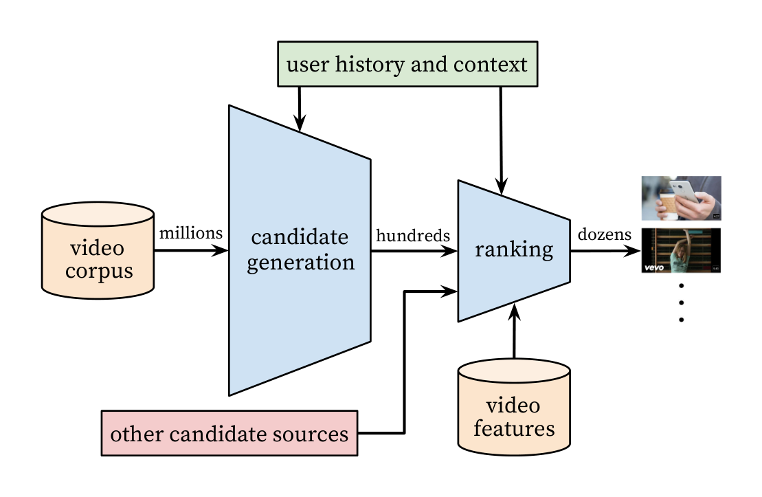
The overall structure of our recommendation system is illustrated in Figure 2. The system is comprised of two neural networks: one for candidate generation and one for ranking.

The candidate generation network takes events from the user’s YouTube activity history as input and retrieves a small subset (hundreds) of videos from a large corpus. These candidates are intended to be generally relevant to the user with high precision. The candidate generation network only provides broad personalization via collaborative filtering. The similarity between users is expressed in terms of coarse features such as IDs of video watches, search query tokens and demographics.

Presenting a few “best” recommendations in a list requires a fine-level representation to distinguish relative importance among candidates with high recall. The ranking network accomplishes this task by assigning a score to each video according to a desired objective function using a rich set of features describing the video and user. The highest scoring videos are presented to the user, ranked by their score.

The two-stage approach to recommendation allows us to make recommendations from a very large corpus (millions) of videos while still being certain that the small number of videos appearing on the device are personalized and engaging for the user. Furthermore, this design enables blending candidates generated by other sources, such as those described in an earlier work [3].

During development, we make extensive use of offline metrics (precision, recall, ranking loss, etc.) to guide iterative improvements to our system. However for the final determination of the effectiveness of an algorithm or model, we rely on A/B testing via live experiments. In a live experiment, we can measure subtle changes in click-through rate, watch time, and many other metrics that measure user engagement. This is important because live A/B results are not always correlated with offline experiments.

3. CANDIDATE GENERATION

Section Summary: The candidate generation stage reduces YouTube’s vast video library to a few hundred potentially relevant items for each user by framing recommendation as a massive classification task. A neural network learns dense embeddings of users and videos from their past watches, search queries, demographics, and other signals, then identifies the most likely next video through efficient sampling during training and fast nearest-neighbor lookup at serving time. This learned approach also incorporates a feature that favors recently uploaded content so the system can surface fresh and emerging videos.

During candidate generation, the enormous YouTube corpus is winnowed down to hundreds of videos that may be relevant to the user. The predecessor to the recommender described here was a matrix factorization approach trained under rank loss [23]. Early iterations of our neural network model mimicked this factorization behavior with shallow networks that only embedded the user’s previous watches. From this perspective, our approach can be viewed as a non-linear generalization of factorization techniques.

3.1 Recommendation as Classification

We pose recommendation as extreme multiclass classification where the prediction problem becomes accurately classifying a specific video watch $w_t$ at time $t$ among millions of videos $i$ (classes) from a corpus $V$ based on a user $U$ and context $C$,

$ P(w_t = i|U, C) = \frac{e^{v_i u}}{\sum_{j \in V} e^{v_j u}} $

where $u \in \mathbb{R}^N$ represents a high-dimensional “embedding” of the user, context pair and the $v_j \in \mathbb{R}^N$ represent embeddings of each candidate video. In this setting, an embedding is simply a mapping of sparse entities (individual videos, users etc.) into a dense vector in $\mathbb{R}^N$. The task of the deep neural network is to learn user embeddings $u$ as a function of the user’s history and context that are useful for discriminating among videos with a softmax classifier.

Although explicit feedback mechanisms exist on YouTube (thumbs up/down, in-product surveys, etc.) we use the implicit feedback [16] of watches to train the model, where a user completing a video is a positive example. This choice is based on the orders of magnitude more implicit user history available, allowing us to produce recommendations deep in the tail where explicit feedback is extremely sparse.

Efficient Extreme Multiclass

To efficiently train such a model with millions of classes, we rely on a technique to sample negative classes from the background distribution (“candidate sampling”) and then correct for this sampling via importance weighting [10]. For each example the cross-entropy loss is minimized for the true label and the sampled negative classes. In practice several thousand negatives are sampled, corresponding to more than 100 times speedup over traditional softmax. A popular alternative approach is hierarchical softmax [15], but we weren’t able to achieve comparable accuracy. In hierarchical softmax, traversing each node in the tree involves discriminating between sets of classes that are often unrelated, making the classification problem much more difficult and degrading performance.

At serving time we need to compute the most likely $N$ classes (videos) in order to choose the top $N$ to present to the user. Scoring millions of items under a strict serving latency of tens of milliseconds requires an approximate scoring scheme sublinear in the number of classes. Previous systems at YouTube relied on hashing [24] and the classifier described here uses a similar approach. Since calibrated likelihoods from the softmax output layer are not needed at serving time, the scoring problem reduces to a nearest neighbor search in the dot product space for which general purpose libraries can be used [12]. We found that A/B results were not particularly sensitive to the choice of nearest neighbor search algorithm.

3.2 Model Architecture

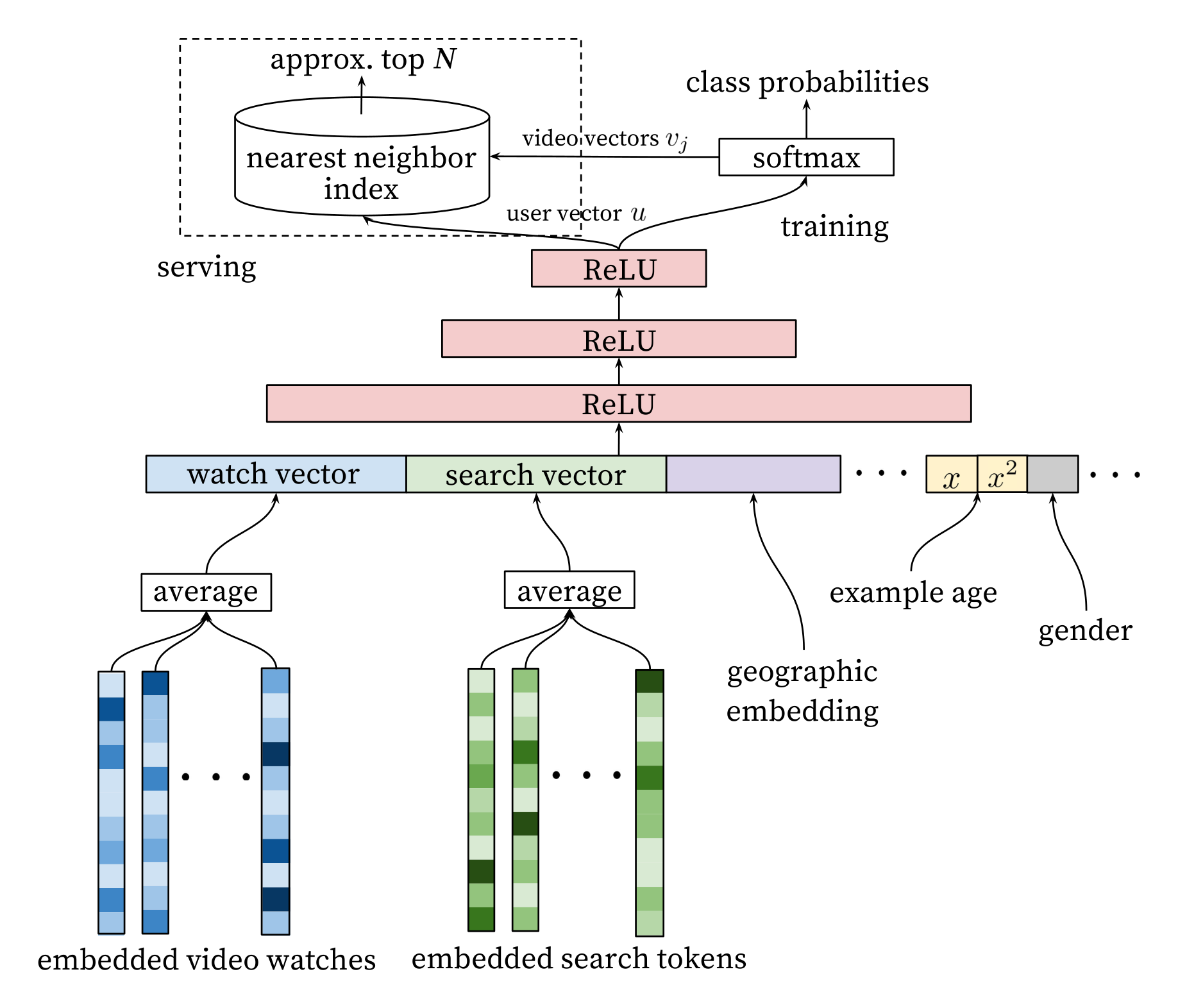
Inspired by continuous bag of words language models [14], we learn high dimensional embeddings for each video in a fixed vocabulary and feed these embeddings into a feedforward neural network. A user’s watch history is represented by a variable-length sequence of sparse video IDs which is mapped to a dense vector representation via the embeddings. The network requires fixed-sized dense inputs and simply averaging the embeddings performed best among several strategies (sum, component-wise max, etc.). Importantly, the embeddings are learned jointly with all other model parameters through normal gradient descent backpropagation updates. Features are concatenated into a wide first layer, followed by several layers of fully connected Rectified Linear Units (ReLU) [6]. Figure 3 shows the general network architecture with additional non-video watch features described below.

3.3 Heterogeneous Signals

A key advantage of using deep neural networks as a generalization of matrix factorization is that arbitrary continuous and categorical features can be easily added to the model. Search history is treated similarly to watch history - each query is tokenized into unigrams and bigrams and each token is embedded. Once averaged, the user’s tokenized, embedded queries represent a summarized dense search history. Demographic features are important for providing priors so that the recommendations behave reasonably for new users. The user’s geographic region and device are embedded and concatenated. Simple binary and continuous features such as the user’s gender, logged-in state and age are input directly into the network as real values normalized to $[0, 1]$.

“Example Age” Feature

Many hours worth of videos are uploaded each second to YouTube. Recommending this recently uploaded (“fresh”) content is extremely important for YouTube as a product. We consistently observe that users prefer fresh content, though not at the expense of relevance. In addition to the first-order effect of simply recommending new videos that users want to watch, there is a critical secondary phenomenon of bootstrapping and propagating viral content [11].

Machine learning systems often exhibit an implicit bias towards the past because they are trained to predict future behavior from historical examples. The distribution of video popularity is highly non-stationary but the multinomial distribution over the corpus produced by our recommender will reflect the average watch likelihood in the training window of several weeks. To correct for this, we feed the age of the training example as a feature during training. At serving time, this feature is set to zero (or slightly negative) to reflect that the model is making predictions at the very end of the training window.

Figure 4 demonstrates the efficacy of this approach on an arbitrarily chosen video [26].

3.4 Label and Context Selection

It is important to emphasize that recommendation often involves solving a surrogate problem and transferring the result to a particular context. A classic example is the assumption that accurately predicting ratings leads to effective movie recommendations [2]. we have found that the choice of this surrogate learning problem has an outsized importance on performance in A/B testing but is very difficult to measure with offline experiments.

Training examples are generated from all YouTube watches (even those embedded on other sites) rather than just watches on the recommendations we produce. Otherwise, it would be very difficult for new content to surface and the recommender would be overly biased towards exploitation. If users are discovering videos through means other than our recommendations, we want to be able to quickly propagate this discovery to others via collaborative filtering. Another key insight that improved live metrics was to generate a fixed number of training examples per user, effectively weighting our users equally in the loss function. This prevented a small cohort of highly active users from dominating the loss.

Somewhat counter-intuitively, great care must be taken to withhold information from the classifier in order to prevent the model from exploiting the structure of the site and overfitting the surrogate problem. Consider as an example a case in which the user has just issued a search query for “taylor swift”. Since our problem is posed as predicting the next watched video, a classifier given this information will predict that the most likely videos to be watched are those which appear on the corresponding search results page for “taylor swift”. Unsurpisingly, reproducing the user’s last search page as homepage recommendations performs very poorly. By discarding sequence information and representing search queries with an unordered bag of tokens, the classifier is no longer directly aware of the origin of the label.

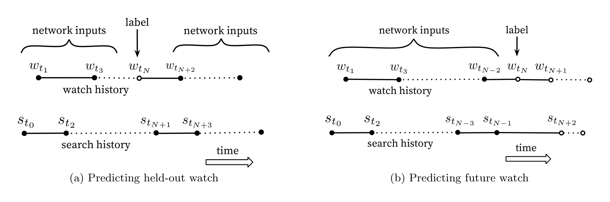
Natural consumption patterns of videos typically lead to very asymmetric co-watch probabilities. Episodic series are usually watched sequentially and users often discover artists in a genre beginning with the most broadly popular before focusing on smaller niches. We therefore found much better performance predicting the user’s next watch, rather than predicting a randomly held-out watch (Figure 5). Many collaborative filtering systems implicitly choose the labels and context by holding out a random item and predicting it from other items in the user’s history (5a). This leaks future information and ignores any asymmetric consumption patterns. In contrast, we “rollback” a user’s history by choosing a random watch and only input actions the user took before the held-out label watch (5b).

3.5 Experiments with Features and Depth

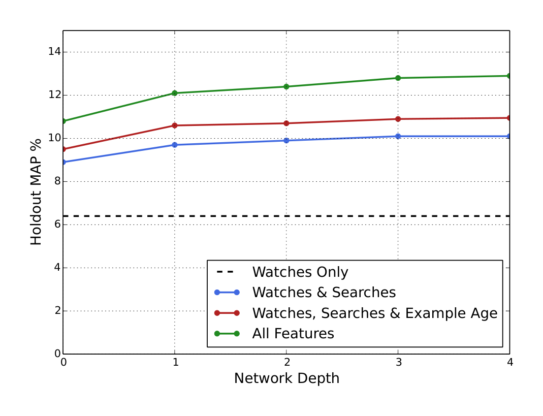
Adding features and depth significantly improves precision on holdout data as shown in Figure 6. In these experiments, a vocabulary of 1M videos and 1M search tokens were embedded with 256 floats each in a maximum bag size of 50 recent watches and 50 recent searches. The softmax layer outputs a multinomial distribution over the same 1M video classes with a dimension of 256 (which can be thought of as a separate output video embedding). These models were trained until convergence over all YouTube users, corresponding to several epochs over the data. Network structure followed a common “tower” pattern in which the bottom of the network is widest and each successive hidden layer halves the number of units (similar to Figure 3). The depth zero network is effectively a linear factorization scheme which performed very similarly to the predecessor system. Width and depth were added until the incremental benefit diminished and convergence became difficult:

• Depth 0: A linear layer simply transforms the concatenation layer to match the softmax dimension of 256
• Depth 1: 256 ReLU
• Depth 2: 512 ReLU $\rightarrow$ 256 ReLU
• Depth 3: 1024 ReLU $\rightarrow$ 512 ReLU $\rightarrow$ 256 ReLU
• Depth 4: 2048 ReLU $\rightarrow$ 1024 ReLU $\rightarrow$ 512 ReLU $\rightarrow$ 256 ReLU

4. RANKING

Section Summary: Ranking uses a deep neural network to assign scores to a few hundred video candidates, sorting them by expected watch time per impression so that the final list shown to the user better matches the specific interface and avoids clickbait. The model draws on hundreds of detailed features that capture both the video itself and the user's past interactions with similar items, allowing it to blend results from multiple candidate sources whose raw scores cannot be compared directly. Categorical features are mapped to dense embeddings that are shared across related signals, while continuous features describe frequencies and recency, all engineered to reflect temporal user behavior.

The primary role of ranking is to use impression data to specialize and calibrate candidate predictions for the particular user interface. For example, a user may watch a given video with high probability generally but is unlikely to click on the specific homepage impression due to the choice of thumbnail image. During ranking, we have access to many more features describing the video and the user’s relationship to the video because only a few hundred videos are being scored rather than the millions scored in candidate generation. Ranking is also crucial for ensembling different candidate sources whose scores are not directly comparable.

We use a deep neural network with similar architecture as candidate generation to assign an independent score to each video impression using logistic regression (Figure 7). The list of videos is then sorted by this score and returned to the user. Our final ranking objective is constantly being tuned based on live A/B testing results but is generally a simple function of expected watch time per impression. Ranking by click-through rate often promotes deceptive videos that the user does not complete (“clickbait”) whereas watch time better captures engagement [13, 25].

4.1 Feature Representation

Our features are segregated with the traditional taxonomy of categorical and continuous/ordinal features. The categorical features we use vary widely in their cardinality - some are binary (e.g. whether the user is logged-in) while others have millions of possible values (e.g. the user’s last search query). Features are further split according to whether they contribute only a single value (“univalent”) or a set of values (“multivalent”). An example of a univalent categorical feature is the video ID of the impression being scored, while a corresponding multivalent feature might be a bag of the last $N$ video IDs the user has watched. We also classify features according to whether they describe properties of the item (“impression”) or properties of the user/context (“query”). Query features are computed once per request while impression features are computed for each item scored.

Feature Engineering

We typically use hundreds of features in our ranking models, roughly split evenly between categorical and continuous. Despite the promise of deep learning to alleviate the burden of engineering features by hand, the nature of our raw data does not easily lend itself to be input directly into feedforward neural networks. We still expend considerable engineering resources transforming user and video data into useful features. The main challenge is in representing a temporal sequence of user actions and how these actions relate to the video impression being scored.

We observe that the most important signals are those that describe a user’s previous interaction with the item itself and other similar items, matching others’ experience in ranking ads [7]. As an example, consider the user’s past history with the channel that uploaded the video being scored - how many videos has the user watched from this channel? When was the last time the user watched a video on this topic? These continuous features describing past user actions on related items are particularly powerful because they generalize well across disparate items. We have also found it crucial to propagate information from candidate generation into ranking in the form of features, e.g. which sources nominated this video candidate? What scores did they assign?

Features describing the frequency of past video impressions are also critical for introducing “churn” in recommendations (successive requests do not return identical lists). If a user was recently recommended a video but did not watch it then the model will naturally demote this impression on the next page load. Serving up-to-the-second impression and watch history is an engineering feat onto itself outside the scope of this paper, but is vital for producing responsive recommendations.

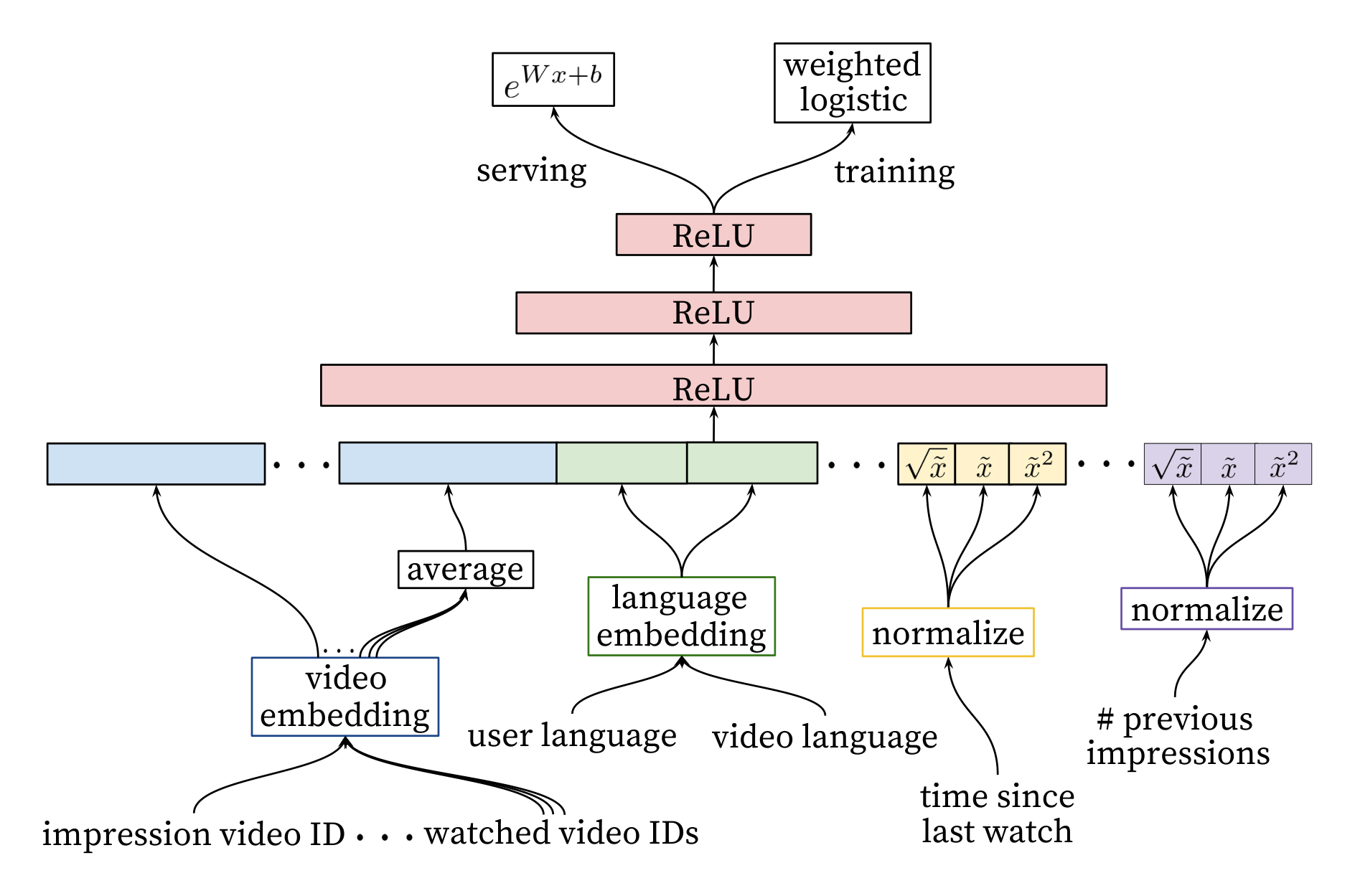
Embedding Categorical Features

Similar to candidate generation, we use embeddings to map sparse categorical features to dense representations suitable for neural networks. Each unique ID space (“vocabulary”) has a separate learned embedding with dimension that increases approximately proportional to the logarithm of the number of unique values. These vocabularies are simple look-up tables built by passing over the data once before training. Very large cardinality ID spaces (e.g. video IDs or search query terms) are truncated by including only the top $N$ after sorting based on their frequency in clicked impressions. Out-of-vocabulary values are simply mapped to the zero embedding. As in candidate generation, multivalent categorical feature embeddings are averaged before being fed in to the network.

Importantly, categorical features in the same ID space also share underlying embeddings. For example, there exists a single global embedding of video IDs that many distinct features use (video ID of the impression, last video ID watched by the user, video ID that “seeded” the recommendation, etc.). Despite the shared embedding, each feature is fed separately into the network so that the layers above can learn specialized representations per feature. Sharing embeddings is important for improving generalization, speeding up training and reducing memory requirements. The overwhelming majority of model parameters are in these high-cardinality embedding spaces - for example, one million IDs embedded in a 32 dimensional space have 7 times more parameters than fully connected layers 2048 units wide.

Normalizing Continuous Features

Neural networks are notoriously sensitive to the scaling and distribution of their inputs [9] whereas alternative approaches such as ensembles of decision trees are invariant to scaling of individual features. We found that proper normalization of continuous features was critical for convergence. A continuous feature $x$ with distribution $f$ is transformed to $\tilde{x}$ by scaling the values such that the feature is equally distributed in $[0, 1)$ using the cumulative distribution, $\tilde{x} = \int_{-\infty}^{x} df$. This integral is approximated with linear interpolation on the quantiles of the feature values computed in a single pass over the data before training begins.

In addition to the raw normalized feature $\tilde{x}$, we also input powers $\tilde{x}^2$ and $\sqrt{\tilde{x}}$, giving the network more expressive power by allowing it to easily form super- and sub-linear functions of the feature. Feeding powers of continuous features was found to improve offline accuracy.

4.2 Modeling Expected Watch Time

Our goal is to predict expected watch time given training examples that are either positive (the video impression was clicked) or negative (the impression was not clicked). Positive examples are annotated with the amount of time the user spent watching the video. To predict expected watch time we use the technique of weighted logistic regression, which was developed for this purpose.

The model is trained with logistic regression under cross-entropy loss (Figure 7). However, the positive (clicked) impressions are weighted by the observed watch time on the video. Negative (unclicked) impressions all receive unit weight. In this way, the odds learned by the logistic regression are $\frac{\sum T_i}{N-k}$ where $N$ is the number of training examples, $k$ is the number of positive impressions, and $T_i$ is the watch time of the $i$th impression. Assuming the fraction of positive impressions is small (which is true in our case), the learned odds are approximately $E[T](1 + P)$, where $P$ is the click probability and $E[T]$ is the expected watch time of the impression. Since $P$ is small, this product is close to $E[T]$. For inference we use the exponential function $e^x$ as the final activation function to produce these odds that closely estimate expected watch time.

4.3 Experiments with Hidden Layers

Table 1 shows the results we obtained on next-day holdout data with different hidden layer configurations. The value shown for each configuration (“weighted, per-user loss”) was obtained by considering both positive (clicked) and negative (unclicked) impressions shown to a user on a single page. We first score these two impressions with our model. If the negative impression receives a higher score than the positive impression, then we consider the positive impression’s watch time to be mispredicted watch time. Weighted, per-user loss is then the total amount mispredicted watch time as a fraction of total watch time over heldout impression pairs.

These results show that increasing the width of hidden layers improves results, as does increasing their depth. The trade-off, however, is server CPU time needed for inference. The configuration of a 1024-wide ReLU followed by a 512-wide ReLU followed by a 256-wide ReLU gave us the best results while enabling us to stay within our serving CPU budget.

For the $1024 \rightarrow 512 \rightarrow 256$ model we tried only feeding the normalized continuous features without their powers, which increased loss by 0.2%. With the same hidden layer configuration, we also trained a model where positive and negative examples are weighted equally. Unsurprisingly, this increased the watch time-weighted loss by a dramatic 4.1%.

: Table 1: Effects of wider and deeper hidden ReLU layers on watch time-weighted pairwise loss computed on next-day holdout data.

\begin{tabular}{|l|c|}
\hline
Hidden layers & weighted, per-user loss \\
\hline
None & 41.6\% \\
256 ReLU & 36.9\% \\
512 ReLU & 36.7\% \\
1024 ReLU & 35.8\% \\
512 ReLU $\rightarrow$ 256 ReLU & 35.2\% \\
1024 ReLU $\rightarrow$ 512 ReLU & 34.7\% \\
1024 ReLU $\rightarrow$ 512 ReLU $\rightarrow$ 256 ReLU & 34.6\% \\
\hline
\end{tabular}

5. CONCLUSIONS

Section Summary: The authors present a deep neural network system for recommending YouTube videos that splits the task into two stages: generating a shortlist of candidates and then ranking them. Their collaborative filtering model captures complex interactions among many signals to outperform earlier matrix factorization methods, aided by careful choices such as predicting a user’s future watch and hiding certain signals so the model generalizes to the live site. For ranking they replace older linear or tree-based techniques with a deep network that incorporates time-aware features and a modified loss function weighting examples by actual watch time, yielding higher accuracy on both offline measures and real-world watch-time metrics.

We have described our deep neural network architecture for recommending YouTube videos, split into two distinct problems: candidate generation and ranking.

Our deep collaborative filtering model is able to effectively assimilate many signals and model their interaction with layers of depth, outperforming previous matrix factorization approaches used at YouTube [23]. There is more art than science in selecting the surrogate problem for recommendations and we found classifying a future watch to perform well on live metrics by capturing asymmetric co-watch behavior and preventing leakage of future information. Withholding disciminative signals from the classifier was also essential to achieving good results - otherwise the model would overfit the surrogate problem and not transfer well to the home page.

We demonstrated that using the age of the training example as an input feature removes an inherent bias towards the past and allows the model to represent the time-dependent behavior of popular videos. This improved offline holdout precision results and increased the watch time dramatically on recently uploaded videos in A/B testing.

Ranking is a more classical machine learning problem yet our deep learning approach outperformed previous linear and tree-based methods for watch time prediction. Recommendation systems in particular benefit from specialized features describing past user behavior with items. Deep neural networks require special representations of categorical and continuous features which we transform with embeddings and quantile normalization, respectively. Layers of depth were shown to effectively model non-linear interactions between hundreds of features.

Logistic regression was modified by weighting training examples with watch time for positive examples and unity for negative examples, allowing us to learn odds that closely model expected watch time. This approach performed much better on watch-time weighted ranking evaluation metrics compared to predicting click-through rate directly.

6. ACKNOWLEDGMENTS

Section Summary: The authors thank Jim McFadden and Pranav Khaitan for their guidance and support on the project. Sujeet Bansal, Shripad Thite, and Radek Vingralek built important parts of the training and serving systems. Chris Berg and Trevor Walker also provided useful discussions and detailed feedback.

The authors would like to thank Jim McFadden and Pranav Khaitan for valuable guidance and support. Sujeet Bansal, Shripad Thite and Radek Vingralek implemented key components of the training and serving infrastructure. Chris Berg and Trevor Walker contributed thoughtful discussion and detailed feedback.

7. REFERENCES

Section Summary: The references section compiles 26 citations drawn mainly from academic papers, conference proceedings, and technical reports. These sources focus on tools and methods for large-scale machine learning, such as the TensorFlow framework, along with research into recommender systems, neural networks, and collaborative filtering. Many entries also describe practical work at companies like YouTube and Facebook on tasks such as video suggestions, click prediction, and measuring user engagement.

[1] M. Abadi, A. Agarwal, P. Barham, E. Brevdo, Z. Chen, C. Citro, G. S. Corrado, A. Davis, J. Dean, M. Devin, S. Ghemawat, I. Goodfellow, A. Harp, G. Irving, M. Isard, Y. Jia, R. Jozefowicz, L. Kaiser, M. Kudlur, J. Levenberg, D. Mané, R. Monga, S. Moore, D. Murray, C. Olah, M. Schuster, J. Shlens, B. Steiner, I. Sutskever, K. Talwar, P. Tucker, V. Vanhoucke, V. Vasudevan, F. Viégas, O. Vinyals, P. Warden, M. Wattenberg, M. Wicke, Y. Yu, and X. Zheng. TensorFlow: Large-scale machine learning on heterogeneous systems, 2015. Software available from tensorflow.org.

[2] X. Amatriain. Building industrial-scale real-world recommender systems. In Proceedings of the Sixth ACM Conference on Recommender Systems, RecSys ’12, pages 7–8, New York, NY, USA, 2012. ACM.

[3] J. Davidson, B. Liebald, J. Liu, P. Nandy, T. Van Vleet, U. Gargi, S. Gupta, Y. He, M. Lambert, B. Livingston, and D. Sampath. The youtube video recommendation system. In Proceedings of the Fourth ACM Conference on Recommender Systems, RecSys ’10, pages 293–296, New York, NY, USA, 2010. ACM.

[4] J. Dean, G. S. Corrado, R. Monga, K. Chen, M. Devin, Q. V. Le, M. Z. Mao, M. Ranzato, A. Senior, P. Tucker, K. Yang, and A. Y. Ng. Large scale distributed deep networks. In NIPS, 2012.

[5] A. M. Elkahky, Y. Song, and X. He. A multi-view deep learning approach for cross domain user modeling in recommendation systems. In Proceedings of the 24th International Conference on World Wide Web, WWW ’15, pages 278–288, New York, NY, USA, 2015. ACM.

[6] X. Glorot, A. Bordes, and Y. Bengio. Deep sparse rectifier neural networks. In G. J. Gordon and D. B. Dunson, editors, Proceedings of the Fourteenth International Conference on Artificial Intelligence and Statistics (AISTATS-11), volume 15, pages 315–323. Journal of Machine Learning Research - Workshop and Conference Proceedings, 2011.

[7] X. He, J. Pan, O. Jin, T. Xu, B. Liu, T. Xu, Y. Shi, A. Atallah, R. Herbrich, S. Bowers, and J. Q. n. Candela. Practical lessons from predicting clicks on ads at facebook. In Proceedings of the Eighth International Workshop on Data Mining for Online Advertising, ADKDD’14, pages 5:1–5:9, New York, NY, USA, 2014. ACM.

[8] W. Huang, Z. Wu, L. Chen, P. Mitra, and C. L. Giles. A neural probabilistic model for context based citation recommendation. In AAAI, pages 2404–2410, 2015.

[9] S. Ioffe and C. Szegedy. Batch normalization: Accelerating deep network training by reducing internal covariate shift. CoRR, abs/1502.03167, 2015.

[10] S. Jean, K. Cho, R. Memisevic, and Y. Bengio. On using very large target vocabulary for neural machine translation. CoRR, abs/1412.2007, 2014.

[11] L. Jiang, Y. Miao, Y. Yang, Z. Lan, and A. G. Hauptmann. Viral video style: A closer look at viral videos on youtube. In Proceedings of International Conference on Multimedia Retrieval, ICMR ’14, pages 193:193–193:200, New York, NY, USA, 2014. ACM.

[12] T. Liu, A. W. Moore, A. Gray, and K. Yang. An investigation of practical approximate nearest neighbor algorithms. pages 825–832. MIT Press, 2004.

[13] E. Meyerson. Youtube now: Why we focus on watch time. http://youtubecreator.blogspot.com/2012/08/youtube-now-why-we-focus-on-watch-time.html. Accessed: 2016-04-20.

[14] T. Mikolov, I. Sutskever, K. Chen, G. Corrado, and J. Dean. Distributed representations of words and phrases and their compositionality. CoRR, abs/1310.4546, 2013.

[15] F. Morin and Y. Bengio. Hierarchical probabilistic neural network language model. In AISTATS, pages 246–252, 2005.

[16] D. Oard and J. Kim. Implicit feedback for recommender systems. In Proceedings of the AAAI Workshop on Recommender Systems, pages 81–83, 1998.

[17] K. J. Oh, W. J. Lee, C. G. Lim, and H. J. Choi. Personalized news recommendation using classified keywords to capture user preference. In 16th International Conference on Advanced Communication Technology, pages 1283–1287, Feb 2014.

[18] S. Sedhain, A. K. Menon, S. Sanner, and L. Xie. Autorec: Autoencoders meet collaborative filtering. In Proceedings of the 24th International Conference on World Wide Web, WWW ’15 Companion, pages 111–112, New York, NY, USA, 2015. ACM.

[19] X. Su and T. M. Khoshgoftaar. A survey of collaborative filtering techniques. Advances in artificial intelligence, 2009:4, 2009.

[20] D. Tang, B. Qin, T. Liu, and Y. Yang. User modeling with neural network for review rating prediction. In Proc. IJCAI, pages 1340–1346, 2015.

[21] A. van den Oord, S. Dieleman, and B. Schrauwen. Deep content-based music recommendation. In C. J. C. Burges, L. Bottou, M. Welling, Z. Ghahramani, and K. Q. Weinberger, editors, Advances in Neural Information Processing Systems 26, pages 2643–2651. Curran Associates, Inc., 2013.

[22] H. Wang, N. Wang, and D.-Y. Yeung. Collaborative deep learning for recommender systems. In Proceedings of the 21th ACM SIGKDD International Conference on Knowledge Discovery and Data Mining, KDD ’15, pages 1235–1244, New York, NY, USA, 2015. ACM.

[23] J. Weston, S. Bengio, and N. Usunier. Wsabie: Scaling up to large vocabulary image annotation. In Proceedings of the International Joint Conference on Artificial Intelligence, IJCAI, 2011.

[24] J. Weston, A. Makadia, and H. Yee. Label partitioning for sublinear ranking. In S. Dasgupta and D. Mcallester, editors, Proceedings of the 30th International Conference on Machine Learning (ICML-13), volume 28, pages 181–189. JMLR Workshop and Conference Proceedings, May 2013.

[25] X. Yi, L. Hong, E. Zhong, N. N. Liu, and S. Rajan. Beyond clicks: Dwell time for personalization. In Proceedings of the 8th ACM Conference on Recommender Systems, RecSys ’14, pages 113–120, New York, NY, USA, 2014. ACM.

[26] Zayn. Pillowtalk. https://www.youtube.com/watch?v=C3d6GntKbk.