A Simple Unified Framework for Detecting Out-of-Distribution Samples and Adversarial Attacks

Kimin Lee$^{1}$, Kibok Lee$^{2}$, Honglak Lee$^{3,2}$, Jinwoo Shin$^{1,4}$

$^{1}$ Korea Advanced Institute of Science and Technology (KAIST)
$^{2}$ University of Michigan
$^{3}$ Google Brain
$^{4}$ AItrics

32nd Conference on Neural Information Processing Systems (NIPS 2018), Montréal, Canada.

Abstract

Detecting test samples drawn sufficiently far away from the training distribution statistically or adversarially is a fundamental requirement for deploying a good classifier in many real-world machine learning applications. However, deep neural networks with the softmax classifier are known to produce highly overconfident posterior distributions even for such abnormal samples. In this paper, we propose a simple yet effective method for detecting any abnormal samples, which is applicable to any pre-trained softmax neural classifier. We obtain the class conditional Gaussian distributions with respect to (low- and upper-level) features of the deep models under Gaussian discriminant analysis, which result in a confidence score based on the Mahalanobis distance. While most prior methods have been evaluated for detecting either out-of-distribution or adversarial samples, but not both, the proposed method achieves the state-of-the-art performances for both cases in our experiments. Moreover, we found that our proposed method is more robust in harsh cases, e.g., when the training dataset has noisy labels or small number of samples. Finally, we show that the proposed method enjoys broader usage by applying it to class-incremental learning: whenever out-of-distribution samples are detected, our classification rule can incorporate new classes well without further training deep models.

Executive Summary: Deep neural networks have transformed applications like image recognition and autonomous vehicles, but they often fail to detect abnormal inputs—such as images from unrelated datasets (out-of-distribution samples) or subtly altered ones designed to fool the system (adversarial attacks). These failures pose serious risks in safety-critical systems, where overconfident predictions on unfamiliar data could lead to errors in self-driving cars or secure authentication. With growing deployment of these networks, reliable detection of such anomalies is urgent to ensure trustworthiness and prevent real-world harm.

This paper proposes and evaluates a straightforward method to detect both out-of-distribution and adversarial samples using any pre-trained neural network classifier, without requiring retraining or access to abnormal data during setup. The goal is to provide a unified, robust confidence score that flags unreliable inputs while preserving the network's original accuracy.

The authors analyzed features from pre-trained convolutional networks like ResNet and DenseNet, trained on common image datasets such as CIFAR-10 (50,000 training images across 10 classes) and SVHN (73,000 digit images). They fitted simple Gaussian distributions to these features per class, using empirical means and a shared covariance from training data. A confidence score was then computed via the Mahalanobis distance—the distance of a test sample to the nearest class distribution—enhanced by minor input perturbations and combining scores from multiple network layers. Experiments covered thousands of test samples over several months of model training, with comparisons to leading methods like ODIN for out-of-distribution detection and LID for adversarial attacks.

Key results show the method's strong performance. First, it detects out-of-distribution samples far better than the top prior approach (ODIN), raising the fraction of correctly flagged abnormal images from 46% to 91% when correctly identifying 95% of normal ones, across datasets like CIFAR-100 versus LSUN scenes. Second, for adversarial attacks (using techniques like fast gradient sign method or Carlini-Wagner), it boosts detection accuracy to 96% area under the curve, compared to 82% for the leading LID method on CIFAR-10. Third, the approach proves more robust: it maintains high performance (over 80% detection) even with noisy training labels (up to 40% random errors) or small datasets (as few as 5,000 samples), and hyperparameters can be tuned solely on normal data plus simple attacks. Fourth, in class-incremental learning—adding new categories over time without full retraining—it achieves 40% higher accuracy than baselines like softmax updates or Euclidean distance classifiers when incorporating 50 new ImageNet classes after CIFAR-100 training.

These findings mean neural networks can now better quantify uncertainty, reducing risks in deployment by alerting users to potential failures rather than proceeding with false confidence. Unlike prior methods that falter on either out-of-distribution or adversarial cases, this unified approach handles both, and its generative modeling unexpectedly matches discriminative classifiers' accuracy without added complexity. This could lower costs for safety checks in production systems and improve compliance in regulated fields like healthcare or finance, where undetected anomalies might cause harm or legal issues.

Leaders should integrate this Mahalanobis-based detector into existing classifiers as a low-effort upgrade, starting with image-based applications. For broader use, pilot tests on domain-specific data (e.g., medical scans) are recommended, weighing the trade-off of minor compute overhead against enhanced reliability. Further work could validate it on non-image tasks or combine it with hybrid inference for even better calibration.

While effective on standard image benchmarks, the method assumes features follow Gaussian patterns, which may limit it in highly diverse or non-vision domains; experiments also relied on specific networks and attacks. Confidence in the results is high for image classification, given consistent outperformance across multiple setups, but users should verify with their own validation data before full reliance.

1. Introduction

Section Summary: Deep neural networks excel at tasks like image classification and speech recognition, but they struggle to reliably measure the uncertainty in their predictions, which is crucial for real-world uses such as self-driving cars and detecting unusual or malicious inputs. This paper introduces a straightforward method that works with any pre-trained neural network to spot out-of-distribution or adversarial samples by calculating distances in the network's feature space, assuming features follow simple Gaussian patterns, without needing to retrain the model. Experiments show this approach outperforms existing techniques in detection accuracy, robustness to noisy data, and even extends to scenarios like adding new classes over time.

Deep neural networks (DNNs) have achieved high accuracy on many classification tasks, e.g., speech recognition ([1]), object detection ([2]) and image classification ([3]). However, measuring the predictive uncertainty still remains a challenging problem ([4, 5]). Obtaining well-calibrated predictive uncertainty is indispensable since it could be useful in many machine learning applications (e.g., active learning ([6]) and novelty detection ([7])) as well as when deploying DNNs in real-world systems ([8]), e.g., self-driving cars and secure authentication system ([9, 10]).

The predictive uncertainty of DNNs is closely related to the problem of detecting abnormal samples that are drawn far away from in-distribution (i.e., distribution of training samples) statistically or adversarially. For detecting out-of-distribution (OOD) samples, recent works have utilized the confidence from the posterior distribution ([11, 5]). For example, [11] proposed the maximum value of posterior distribution from the classifier as a baseline method, and it is improved by processing the input and output of DNNs ([5]). For detecting adversarial samples, confidence scores were proposed based on density estimators to characterize them in feature spaces of DNNs ([12]). More recently, [13] proposed the local intrinsic dimensionality (LID) and empirically showed that the characteristics of test samples can be estimated effectively using the LID. However, most prior works on this line typically do not evaluate both OOD and adversarial samples. To best of our knowledge, no universal detector is known to work well on both tasks.

Contribution. In this paper, we propose a simple yet effective method, which is applicable to any pre-trained softmax neural classifier (without re-training) for detecting abnormal test samples including OOD and adversarial ones. Our high-level idea is to measure the probability density of test sample on feature spaces of DNNs utilizing the concept of a "generative" (distance-based) classifier. Specifically, we assume that pre-trained features can be fitted well by a class-conditional Gaussian distribution since its posterior distribution can be shown to be equivalent to the softmax classifier under Gaussian discriminant analysis (see Section 2.1 for our justification). Under this assumption, we define the confidence score using the Mahalanobis distance with respect to the closest class-conditional distribution, where its parameters are chosen as empirical class means and tied empirical covariance of training samples. To the contrary of conventional beliefs, we found that using the corresponding generative classifier does not sacrifice the softmax classification accuracy. Perhaps surprisingly, its confidence score outperforms softmax-based ones very strongly across multiple other tasks: detecting OOD samples, detecting adversarial samples and class-incremental learning.

We demonstrate the effectiveness of the proposed method using deep convolutional neural networks, such as DenseNet ([14]) and ResNet ([3]) trained for image classification tasks on various datasets including CIFAR ([15]), SVHN ([16]), ImageNet ([17]) and LSUN ([18]). First, for the problem of detecting OOD samples, the proposed method outperforms the current state-of-the-art method, ODIN ([5]), in all tested cases. In particular, compared to ODIN, our method improves the true negative rate (TNR), i.e., the fraction of detected OOD (e.g., LSUN) samples, from $45.6%$ to $90.9%$ on ResNet when 95% of in-distribution (e.g., CIFAR-100) samples are correctly detected. Next, for the problem of detecting adversarial samples, e.g., generated by four attack methods such as FGSM ([19]), BIM ([20]), DeepFool ([21]) and CW ([22]), our method outperforms the state-of-the-art detection measure, LID ([13]). In particular, compared to LID, ours improves the TNR of CW from $82.9%$ to $95.8%$ on ResNet when 95% of normal CIFAR-10 samples are correctly detected.

We also found that our proposed method is more robust in the choice of its hyperparameters as well as against extreme scenarios, e.g., when the training dataset has some noisy, random labels or a small number of data samples. In particular, [5] tune the hyperparameters of ODIN using validation sets of OOD samples, which is often impossible since the knowledge about OOD samples is not accessible a priori. We show that hyperparameters of the proposed method can be tuned only using in-distribution (training) samples, while maintaining its performance. We further show that the proposed method tuned on a simple attack, i.e., FGSM, can be used to detect other more complex attacks such as BIM, DeepFool and CW.

Finally, we apply our method to class-incremental learning ([23]): new classes are added progressively to a pre-trained classifier. Since the new class samples are drawn from an out-of-training distribution, it is natural to expect that one can classify them using our proposed metric without re-training the deep models. Motivated by this, we present a simple method which accommodates a new class at any time by simply computing the class mean of the new class and updating the tied covariance of all classes. We show that the proposed method outperforms other baseline methods, such as Euclidean distance-based classifier and re-trained softmax classifier. This evidences that our approach have a potential to apply to many other related machine learning tasks, such as active learning ([6]), ensemble learning ([24]) and few-shot learning ([25]).

2. Mahalanobis distance-based score from generative classifier

Section Summary: Researchers have developed a straightforward way to spot unusual images, like those from outside the training data or tampered by adversaries, using deep neural networks originally trained with a standard softmax classifier. They treat the network's internal feature representations as coming from separate Gaussian distributions for each class, calculating class averages and a shared spread from training examples to fit these distributions without retraining the network. A confidence score is then computed as the negative Mahalanobis distance—essentially how far an input's features are from the nearest class distribution, accounting for spread—which proves more reliable than simpler measures and matches the network's accuracy on normal data while highlighting abnormalities.

Given deep neural networks (DNNs) with the softmax classifier, we propose a simple yet effective method for detecting abnormal samples such as out-of-distribution (OOD) and adversarial ones. We first present the proposed confidence score based on an induced generative classifier under Gaussian discriminant analysis (GDA), and then introduce additional techniques to improve its performance. We also discuss how the confidence score is applicable to incremental learning.

2.1 Why Mahalanobis distance-based score?

Derivation of generative classifiers from softmax ones. Let $\mathbf{x}\in \mathcal{X}$ be an input and $y \in \mathcal{Y} = {1, \cdots, C}$ be its label. Suppose that a pre-trained softmax neural classifier is given: $P\left(y=c|\mathbf{x}\right) = \frac{ \exp \left(\mathbf{w}c^\top f \left(\mathbf{x} \right) + b_c \right) }{\sum{c^\prime} \exp \left(\mathbf{w}{c^\prime}^\top f \left(\mathbf{x} \right) + b{c^\prime}\right) }, $ where $\mathbf{w}_c$ and $b_c$ are the weight and the bias of the softmax classifier for class $c$, and $f(\cdot)$ denotes the output of the penultimate layer of DNNs. Then, without any modification on the pre-trained softmax neural classifier, we obtain a generative classifier assuming that a class-conditional distribution follows the multivariate Gaussian distribution. Specifically, we define $C$ class-conditional Gaussian distributions with a tied covariance $\mathbf{\Sigma}$: $P\left(f(\mathbf{x})|y=c\right) = \mathcal{N} \left(f(\mathbf{x})| \mathbf{\mu}_c, \mathbf{\Sigma} \right), $ where $\mathbf{\mu}_c$ is the mean of multivariate Gaussian distribution of class $c \in {1, ..., C}$. Here, our approach is based on a simple theoretical connection between GDA and the softmax classifier: the posterior distribution defined by the generative classifier under GDA with tied covariance assumption is equivalent to the softmax classifier (see the supplementary material for more details). Therefore, the pre-trained features of the softmax neural classifier $f(\mathbf{x})$ might also follow the class-conditional Gaussian distribution.

To estimate the parameters of the generative classifier from the pre-trained softmax neural classifier, we compute the empirical class mean and covariance of training samples ${(\mathbf{x}_1, y_1), \ldots, (\mathbf{x}_N, y_N)}$:

$ \begin{align} {\widehat{\mu}}c = \frac{1}{N_c} \sum{i:y_i=c} f(\mathbf{x}i), ; \mathbf{\widehat{\Sigma}} = \frac{1}{N} \sum_c \sum{i:y_i=c} \left(f(\mathbf{x}_i) - \widehat{\mu}_c\right) \left(f(\mathbf{x}_i) - \widehat{\mu}_c\right)^\top, \end{align}\tag{1} $

where $N_c$ is the number of training samples with label $c$. This is equivalent to fitting the class-conditional Gaussian distributions with a tied covariance to training samples under the maximum likelihood estimator.

Mahalanobis distance-based confidence score. Using the above induced class-conditional Gaussian distributions, we define the confidence score $M(\mathbf{x})$ using the Mahalanobis distance between test sample $\mathbf{x}$ and the closest class-conditional Gaussian distribution, i.e.,

$ \begin{align} M(\mathbf{x}) = \max_c ~ - \left(f(\mathbf{x}) - {\widehat{\mu}}{c} \right)^\top \mathbf{\widehat{\Sigma}}^{-1} \left(f(\mathbf{x}) - {\widehat{\mu}}{c}\right). \end{align}\tag{2} $

Note that this metric corresponds to measuring the log of the probability densities of the test sample. Here, we remark that abnormal samples can be characterized better in the representation space of DNNs, rather than the "label-overfitted" output space of softmax-based posterior distribution used in the prior works [11, 5] for detecting them. It is because a confidence measure obtained from the posterior distribution can show high confidence even for abnormal samples that lie far away from the softmax decision boundary. [12] and [13] process the DNN features for detecting adversarial samples in a sense, but do not utilize the Mahalanobis distance-based metric, i.e., they only utilize the Euclidean distance in their scores. In this paper, we show that Mahalanobis distance is significantly more effective than the Euclidean distance in various tasks.

Experimental supports for generative classifiers. To evaluate our hypothesis that trained features of DNNs support the assumption of GDA, we measure the classification accuracy as follows:

$ \begin{align} \widehat{y} (\mathbf{x}) = \arg \min_c \left(f(\mathbf{x}) - {\widehat{\mu}}{c} \right)^\top \mathbf{\widehat{\Sigma}}^{-1} \left(f(\mathbf{x}) - {\widehat{\mu}}{c}\right). \end{align}\tag{3} $

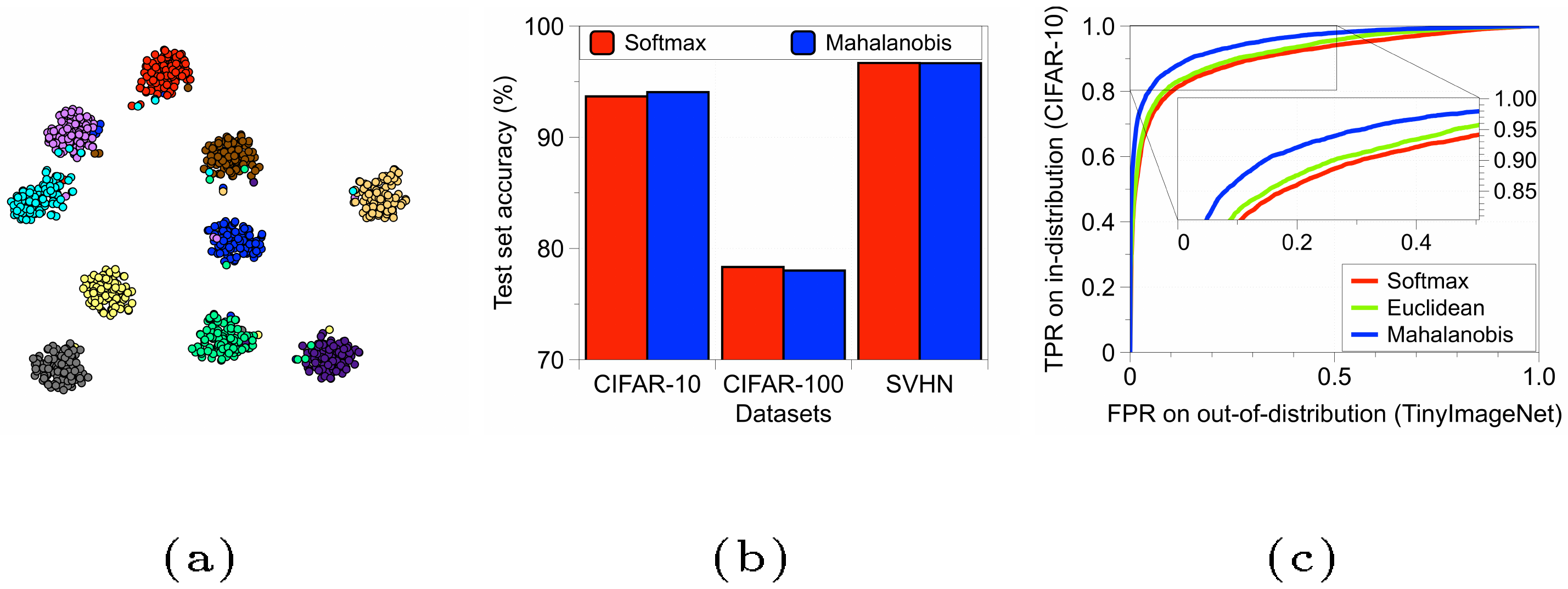
We remark that this corresponds to predicting a class label using the posterior distribution from generative classifier with the uniform class prior. Interestingly, we found that the softmax accuracy (red bar) is also achieved by the Mahalanobis distance-based classifier (blue bar), while conventional knowledge is that a generative classifier trained from scratch typically performs much worse than a discriminative classifier such as softmax. For visual interpretation, Figure 1a presents embeddings of final features from CIFAR-10 test samples constructed by t-SNE ([26]), where the colors of points indicate the classes of the corresponding objects. One can observe that all ten classes are clearly separated in the embedding space, which supports our intuition. In addition, we also show that Mahalanobis distance-based metric can be very useful in detecting out-of-distribution samples. For evaluation, we obtain the receiver operating characteristic (ROC) curve using a simple threshold-based detector by computing the confidence score $M(\mathbf{x})$ on a test sample $\mathbf{x}$ and decide it as positive (i.e., in-distribution) if $M(\mathbf{x})$ is above some threshold. The Euclidean distance, which only utilizes the empirical class means, is considered for comparison. We train ResNet on CIFAR-10, and TinyImageNet dataset ([17]) is used for an out-of-distribution. As shown in Figure 1c, the Mahalanobis distance-based metric (blue bar) performs better than Euclidean one (green bar) and the maximum value of the softmax distribution (red bar).

Input: Test sample $\mathbf{x}$, weights of logistic regression detector $\alpha_\ell$, noise $\varepsilon$ and parameters of Gaussian distributions $\{ {\widehat{\mu}}_{\ell,c}, \mathbf{\widehat{\Sigma}}_\ell: \forall \ell,c \}$
---
Initialize score vectors: $\mathbf{M}(\mathbf{x}) = [M_\ell:\forall \ell]$
**for** each layer $\ell \in 1,\ldots,L$ **do**
  Find the closest class: $\widehat{c} = \arg \min_c ~(f_\ell(\mathbf{x}) - \mathbf{\widehat{\mu}}_{\ell,c})^\top \mathbf{\widehat{\Sigma}_\ell}^{-1} (f_\ell(\mathbf{x}) - \mathbf{\widehat{\mu}}_{\ell,c})$
  Add small noise to test sample: $\mathbf{\widehat{x}} = \mathbf{x} - \varepsilon sign \left( \bigtriangledown_{\mathbf{x}} \left( f_\ell(\mathbf{x}) - {\widehat{\mu}}_{\ell, \widehat{c}}\right)^\top \mathbf{\widehat{\Sigma}_\ell}^{-1} \left( f_\ell(\mathbf{x}) - {\widehat{\mu}}_{\ell,\widehat{c}}\right) \right)$
  Computing confidence score: $M_\ell = \max \limits_c  - \left(f_\ell(\mathbf{\widehat{x}}) - \mathbf{\widehat{\mu}}_{\ell,c}\right)^\top \mathbf{\widehat{\Sigma}_\ell}^{-1} \left(f_\ell(\mathbf{\widehat{x}}) - \mathbf{\widehat{\mu}}_{\ell, c}\right)$
**end for**
**return** Confidence score for test sample {$\sum_{\ell} \alpha_\ell M_\ell$}

2.2 Calibration techniques

Input pre-processing. To make in- and out-of-distribution samples more separable, we consider adding a small controlled noise to a test sample. Specifically, for each test sample $\mathbf{x}$, we calculate the pre-processed sample $\mathbf{\widehat{x}}$ by adding the small perturbations as follows:

$ \begin{align} \mathbf{\widehat{x}} = \mathbf{x} + \varepsilon \text{sign} \left(\bigtriangledown_{\mathbf{x}} M(\mathrm{x}) \right) = \mathbf{x} - \varepsilon \text{sign} \left(\bigtriangledown_{\mathbf{x}} \left(f(\mathbf{x}) - {\widehat{\mu}}{\widehat{c}}\right)^\top \mathbf{\widehat{\Sigma}}^{-1} \left(f(\mathbf{x}) - {\widehat{\mu}}{\widehat{c}}\right) \right), \end{align}\tag{4} $

where $\varepsilon$ is a magnitude of noise and $\widehat{c}$ is the index of the closest class. Next, we measure the confidence score using the pre-processed sample. We remark that the noise is generated to increase the proposed confidence score Equation 2 unlike adversarial attacks ([19]). In our experiments, such perturbation can have stronger effect on separating the in- and out-of-distribution samples. We remark that similar input pre-processing was studied in ([5]), where the perturbations are added to increase the softmax score of the predicted label. However, our method is different in that the noise is generated to increase the proposed metric.

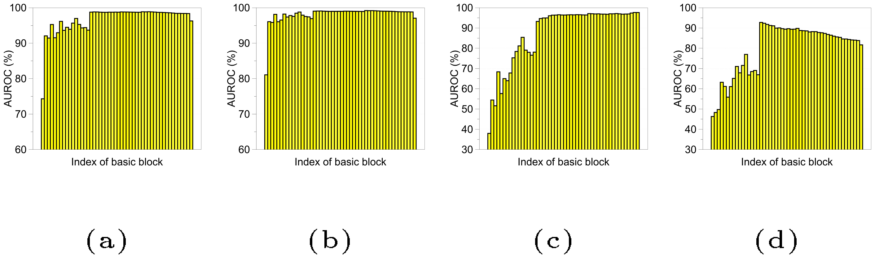
Feature ensemble. To further improve the performance, we consider measuring and combining the confidence scores from not only the final features but also the other low-level features in DNNs. Formally, given training data, we extract the $\ell$-th hidden features of DNNs, denoted by $f_{\ell}(\mathbf{x})$, and compute their empirical class means and tied covariances, i.e., ${\widehat{\mu}}{\ell, c}$ and $\mathbf{\widehat{\Sigma}}\ell$. Then, for each test sample $\mathbf{x}$, we measure the confidence score from the $\ell$-th layer using the formula in Equation 2. One can expect that this simple but natural scheme can bring an extra gain in obtaining a better calibrated score by extracting more input-specific information from the low-level features. We measure the area under ROC (AUROC) curves of the threshold-based detector using the confidence score in Equation 2 computed at different basic blocks of DenseNet ([14]) trained on CIFAR-10 dataset, where the overall trends on ResNet are similar. Figure 2 shows the performance on various OOD samples such as SVHN ([16]), LSUN ([18]), TinyImageNet and adversarial samples generated by DeepFool ([21]), where the dimensions of the intermediate features are reduced using average pooling (see Section 3 for more details). As shown in Figure 2, the confidence scores computed at low-level features often provide better calibrated ones compared to final features (e.g., LSUN, TinyImageNet and DeepFool). To further improve the performance, we design a feature ensemble method as described in Algorithm 1. We first extract the confidence scores from all layers, and then integrate them by weighted averaging: $\sum_{\ell} \alpha_\ell M_\ell(\mathbf{x})$, where $M_\ell(\cdot)$ and $\alpha_\ell$ is the confidence score at the $\ell$-th layer and its weight, respectively. In our experiments, following similar strategies in ([13]), we choose the weight of each layer $\alpha_\ell$ by training a logistic regression detector using validation samples. We remark that such weighted averaging of confidence scores can prevent the degradation on the overall performance even in the case when the confidence scores from some layers are not effective: the trained weights (using validation) would be nearly zero for those ineffective layers.

Input: set of samples from a new class $\{ \mathbf{x}_i : \forall i = 1 \dots N_{C+1} \}$, mean and covariance of observed classes $\{  \widehat{\mathbf{\mu}}_c: \forall c = 1 \dots C \},  \widehat{\mathbf{\Sigma}}$
---
Compute the new class mean: $ \widehat{\mathbf{\mu}}_{C+1} \leftarrow \frac{1}{N_{C+1}} \sum_i f(\mathbf{x}_i)$
Compute the covariance of the new class: $ \widehat{\mathbf{\Sigma}}_{C+1} \leftarrow \frac{1}{N_{C+1}} \sum_i (f(\mathbf{x}_i) -  \widehat{\mathbf{\mu}}_{C+1}) (f(\mathbf{x}_i) -  \widehat{\mathbf{\mu}}_{C+1})^\top$
Update the shared covariance: $ \widehat{\mathbf{\Sigma}} \leftarrow \frac{C}{C+1} \widehat{\mathbf{\Sigma}} + \frac{1}{C+1} \widehat{\mathbf{\Sigma}}_{C+1}$
**return** Mean and covariance of all classes $\{  \widehat{\mathbf{\mu}}_c: \forall c = 1 \dots C+1 \},  \widehat{\mathbf{\Sigma}}$

2.3 Class-incremental learning using Mahalanobis distance-based score

As a natural extension, we also show that the Mahalanobis distance-based confidence score can be utilized in class-incremental learning tasks ([23]): a classifier pre-trained on base classes is progressively updated whenever a new class with corresponding samples occurs. This task is known to be challenging since one has to deal with catastrophic forgetting ([27]) with a limited memory. To this end, recent works have been toward developing new training methods which involve a generative model or data sampling, but adopting such training methods might incur expensive back-and-forth costs. Based on the proposed confidence score, we develop a simple classification method without the usage of complicated training methods. To do this, we first assume that the classifier is well pre-trained with a certain amount of base classes, where the assumption is quite reasonable in many practical scenarios.[^1] In this case, one can expect that not only the classifier can detect OOD samples well, but also might be good for discriminating new classes, as the representation learned with the base classes can characterize new ones. Motivated by this, we present a Mahalanobis distance-based classifier based on Equation 3, which tries to accommodate a new class by simply computing and updating the class mean and covariance, as described in Algorithm 2. The class-incremental adaptation of our confidence score shows its potential to be applied to a wide range of new applications in the future.

[^1]: For example, state-of-the-art CNNs trained on large-scale image dataset are off-the-shelf ([3, 14]), so they are a starting point in many computer vision tasks ([2, 7, 28]).

3. Experimental results

Section Summary: The experimental results section shows how a new method for detecting out-of-distribution images—those that don't match the training data—works well using advanced neural networks like DenseNet and ResNet on common image datasets such as CIFAR, SVHN, and others. By combining features from different parts of the network and preprocessing inputs, the approach outperforms simpler baselines and a leading technique called ODIN, particularly in accurately spotting unusual images while correctly identifying most normal ones, with improvements like raising detection rates from 41% to 91% in some cases. The method also proves robust in tough scenarios, such as when tuning it with fake adversarial examples instead of real outliers or under limited or noisy training data.

In this section, we demonstrate the effectiveness of the proposed method using deep convolutional neural networks such as DenseNet ([14]) and ResNet ([3]) on various vision datasets: CIFAR ([15]), SVHN ([16]), ImageNet ([17]) and LSUN ([18]). Due to the space limitation, we provide the more detailed experimental setups and results in the supplementary material. Our code is available at https://github.com/pokaxpoka/deep_Mahalanobis_detector.

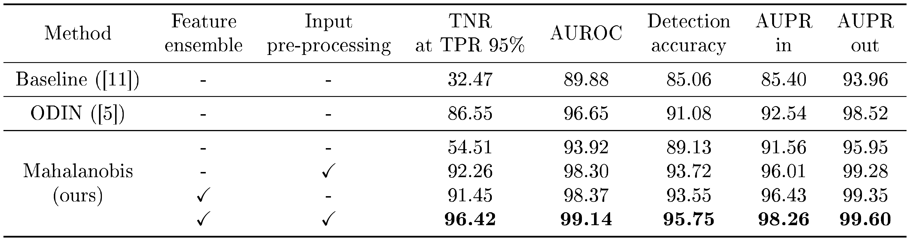
::: {caption="Table 1: Contribution of each proposed method on distinguishing in- and out-of-distribution test set data. We measure the detection performance using ResNet trained on CIFAR-10, when SVHN dataset is used as OOD. All values are percentages and the best results are indicated in bold."}

:::

3.1 Detecting out-of-distribution samples

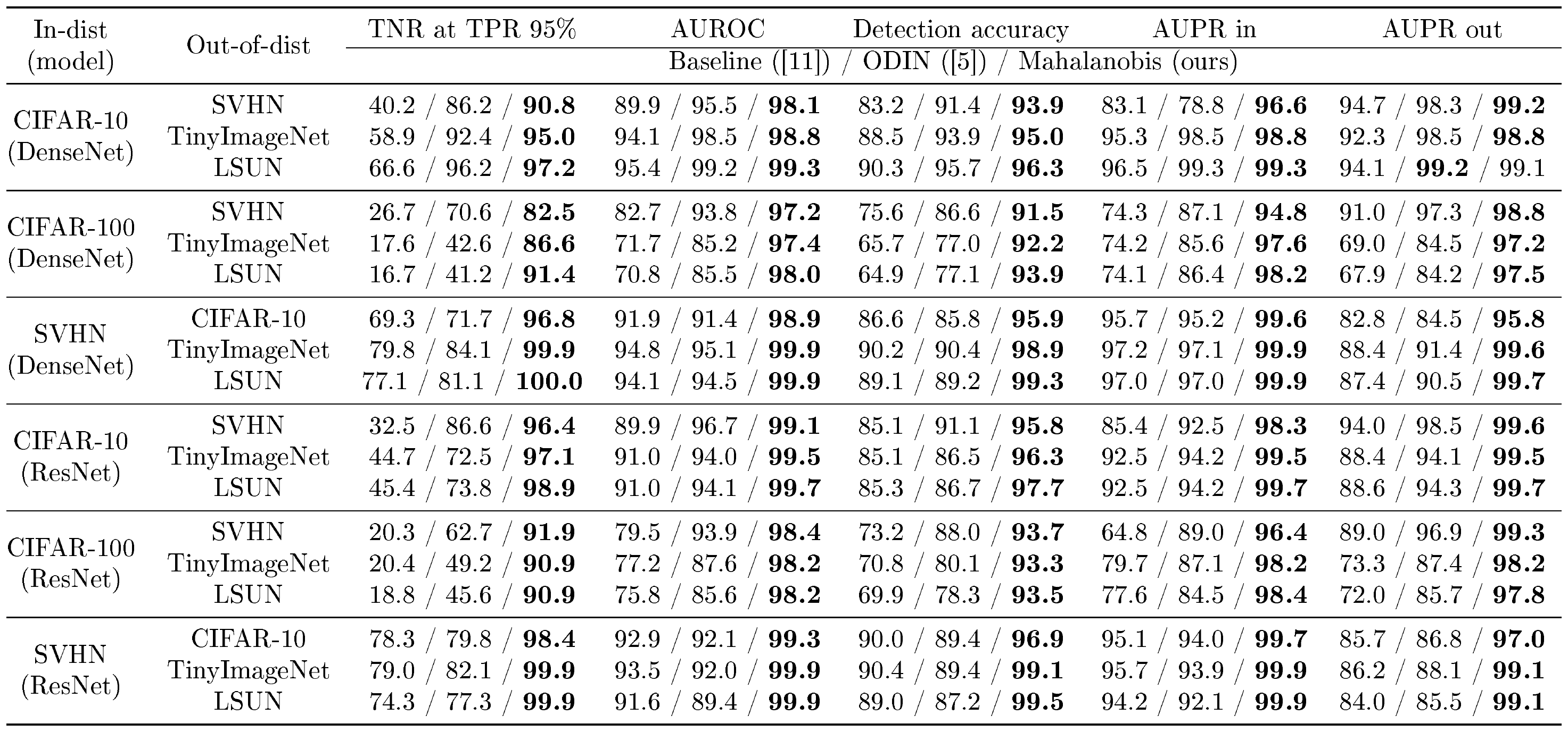
Setup. For the problem of detecting out-of-distribution (OOD) samples, we train DenseNet with 100 layers and ResNet with 34 layers for classifying CIFAR-10, CIFAR-100 and SVHN datasets. The dataset used in training is the in-distribution (positive) dataset and the others are considered as OOD (negative). We only use test datasets for evaluation. In addition, the TinyImageNet (i.e., subset of ImageNet dataset) and LSUN datasets are also tested as OOD. For evaluation, we use a threshold-based detector which measures some confidence score of the test sample, and then classifies the test sample as in-distribution if the confidence score is above some threshold. We measure the following metrics: the true negative rate (TNR) at 95% true positive rate (TPR), the area under the receiver operating characteristic curve (AUROC), the area under the precision-recall curve (AUPR), and the detection accuracy. For comparison, we consider the baseline method ([11]), which defines a confidence score as a maximum value of the posterior distribution, and the state-of-the-art ODIN ([5]), which defines the confidence score as a maximum value of the processed posterior distribution.

For our method, we extract the confidence scores from every end of dense (or residual) block of DenseNet (or ResNet). The size of feature maps on each convolutional layers is reduced by average pooling for computational efficiency: $\mathcal{F} \times \mathcal{H} \times \mathcal{W} \rightarrow \mathcal{F} \times 1$, where $\mathcal{F}$ is the number of channels and $\mathcal{H} \times \mathcal{W}$ is the spatial dimension. As shown in Algorithm 1, the output of the logistic regression detector is used as the final confidence score in our case. All hyperparameters are tuned on a separate validation set, which consists of 1, 000 images from each in- and out-of-distribution pair. Similar to [13], the weights of logistic regression detector are trained using nested cross validation within the validation set, where the class label is assigned positive for in-distribution samples and assigned negative for OOD samples. Since one might not have OOD validation datasets in practice, we also consider tuning the hyperparameters using in-distribution (positive) samples and corresponding adversarial (negative) samples generated by FGSM ([19]).

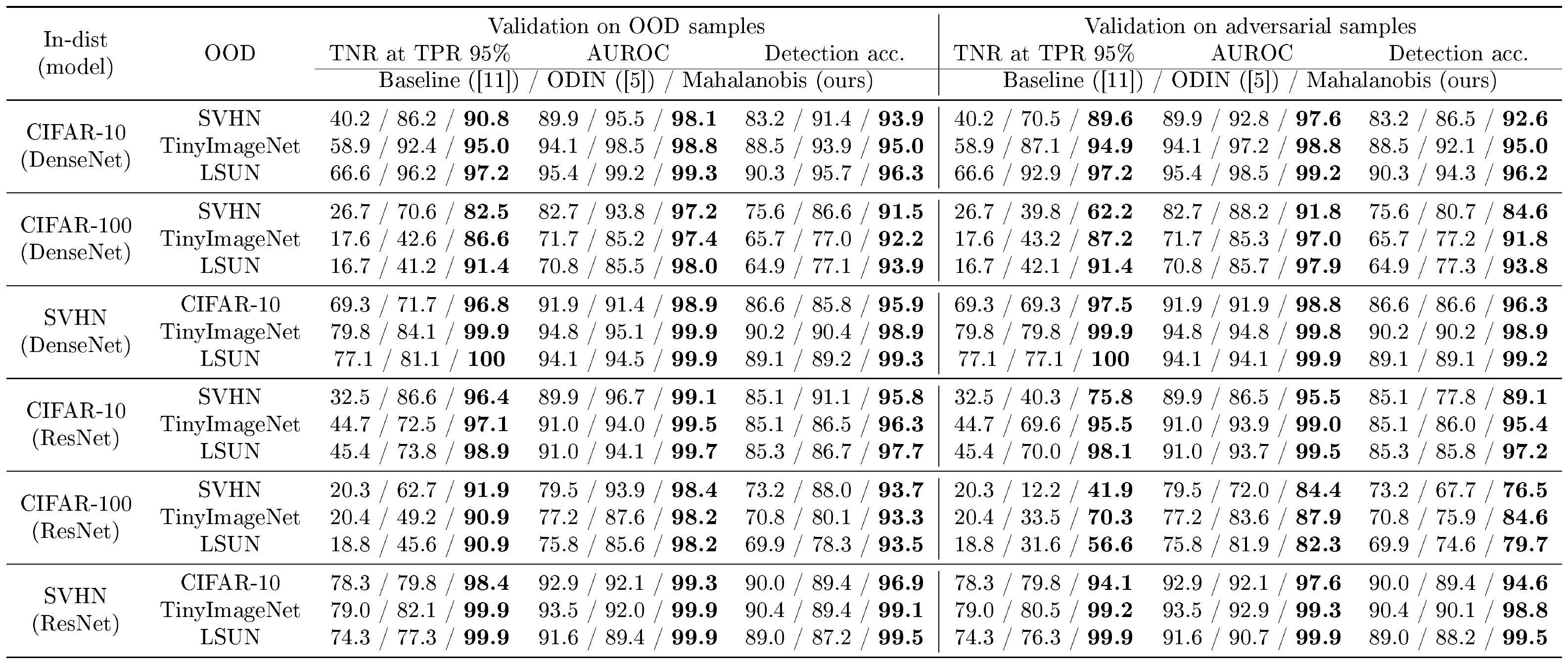
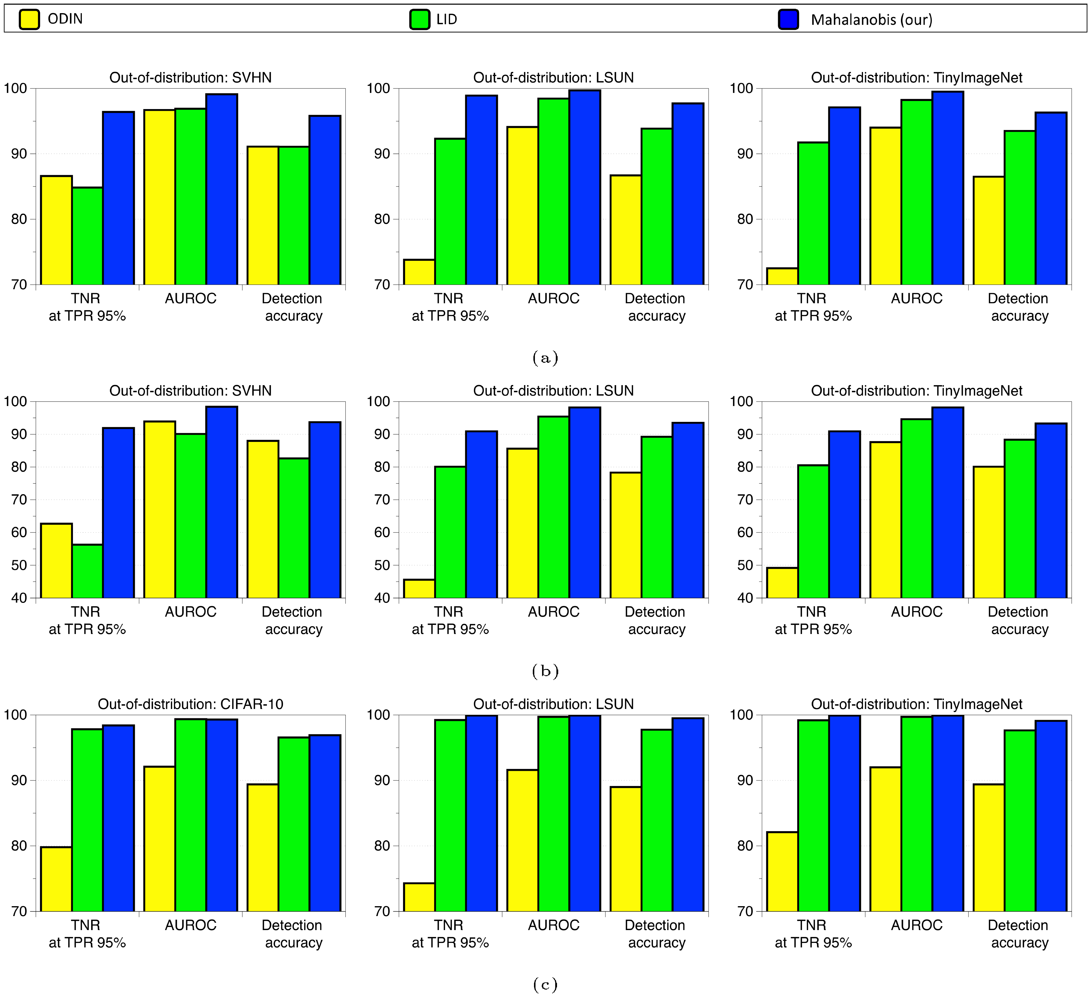
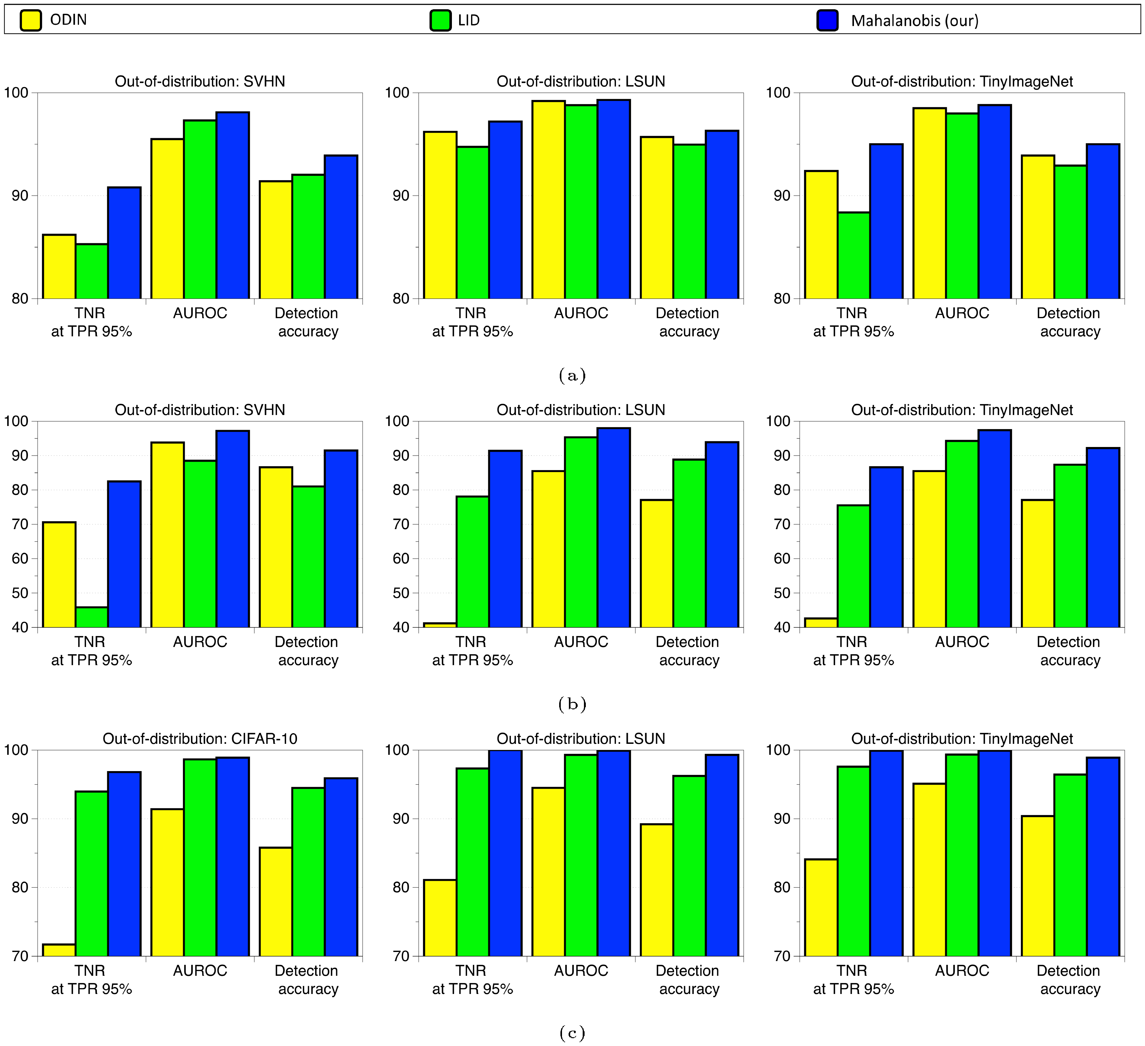
Contribution by each technique and comparison with ODIN. Table 1 validates the contributions of our suggested techniques under the comparison with the baseline method and ODIN. We measure the detection performance using ResNet trained on CIFAR-10, when SVHN dataset is used as OOD. We incrementally apply our techniques to see the stepwise improvement by each component. One can note that our method significantly outperforms the baseline method without feature ensembles and input pre-processing. This implies that our method can characterize the OOD samples very effectively compared to the posterior distribution. By utilizing the feature ensemble and input pre-processing, the detection performance are further improved compared to that of ODIN. The left-hand column of Table 2 reports the detection performance with ODIN for all in- and out-of-distribution dataset pairs. Our method outperforms the baseline and ODIN for all tested cases. In particular, our method improves the TNR, i.e., the fraction of detected LSUN samples, compared to ODIN: $41.2%\rightarrow 91.4%$ using DenseNet, when 95% of CIFAR-100 samples are correctly detected.

::: {caption="Table 2: Distinguishing in- and out-of-distribution test set data for image classification under various validation setups. All values are percentages and the best results are indicated in bold."}

:::

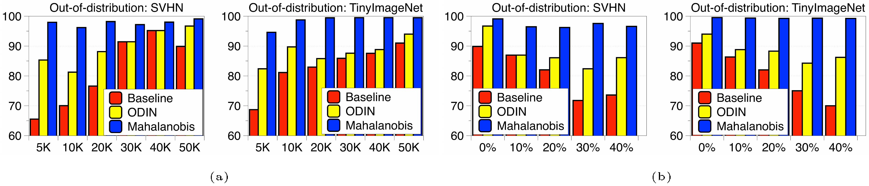
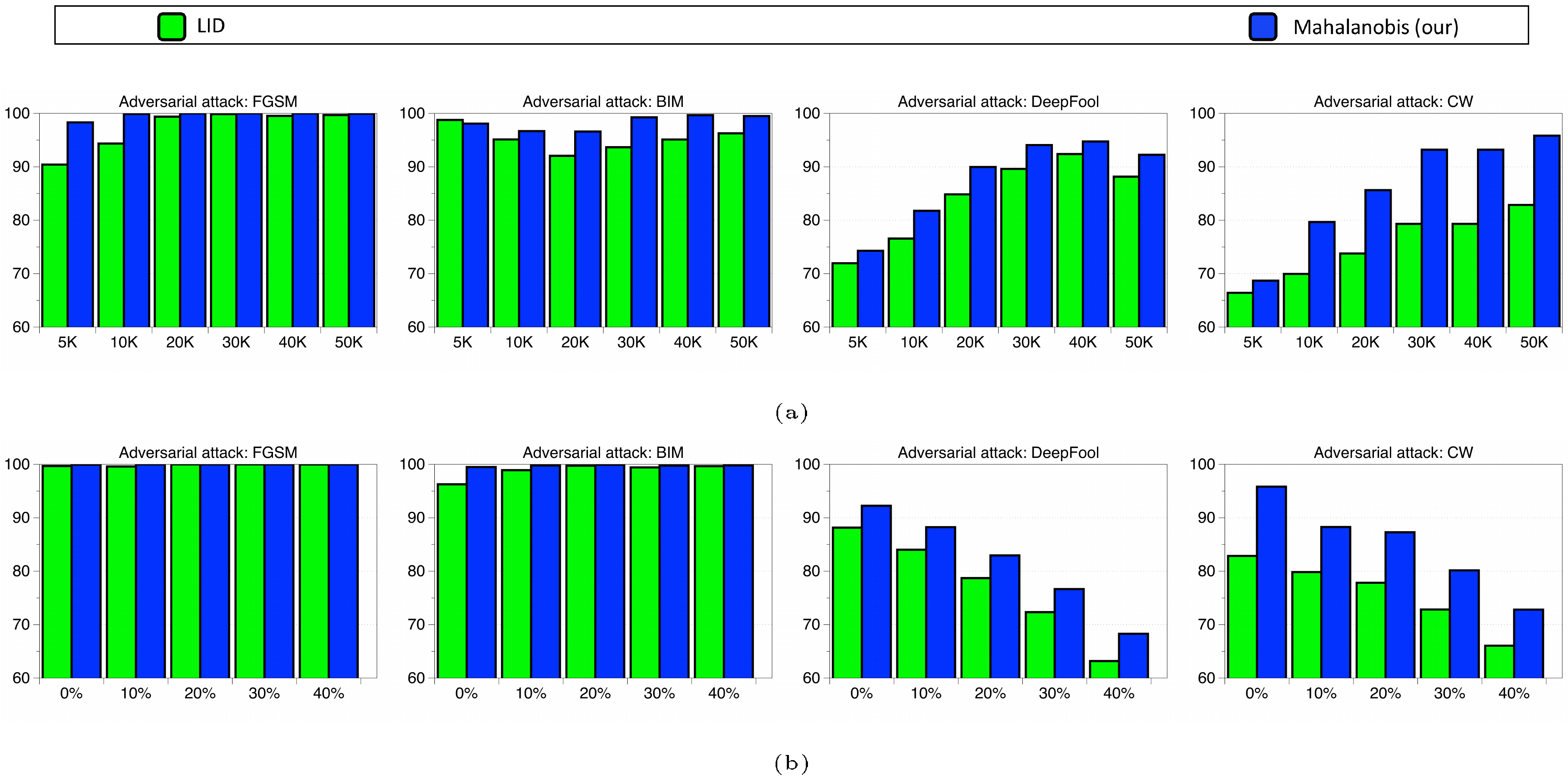
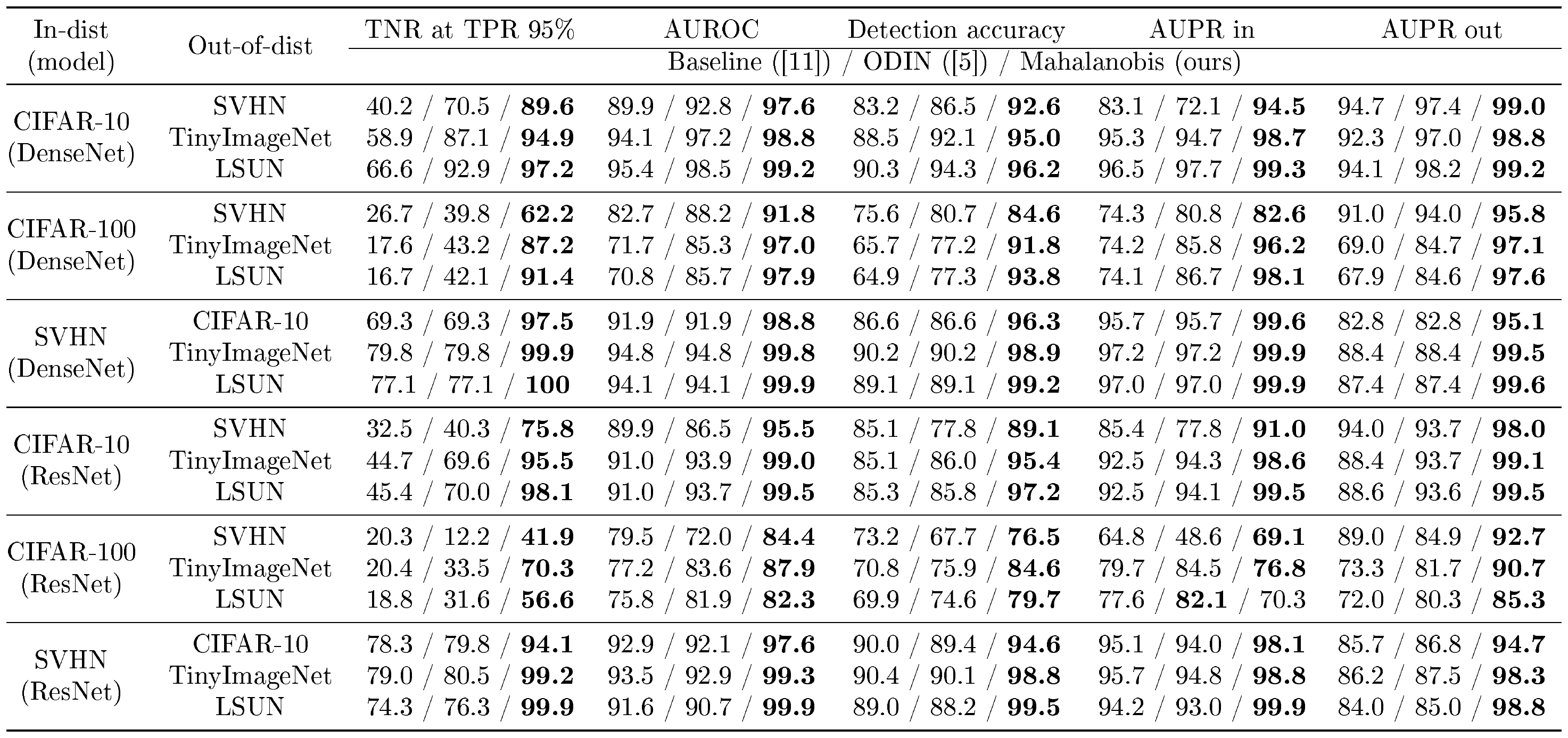
Comparison of robustness. In order to evaluate the robustness of our method, we measure the detection performance when all hyperparameters are tuned only using in-distribution and adversarial samples generated by FGSM ([19]). As shown in the right-hand column of Table 2, ODIN is working poorly compared to the baseline method in some cases (e.g., DenseNet trained on SVHN), while our method still outperforms the baseline and ODIN consistently. We remark that our method validated without OOD but adversarial samples even outperforms ODIN validated with OOD. We also verify the robustness of our method under various training setups. Since our method utilizes empirical class mean and covariance of training samples, there is a caveat such that it can be affected by the properties of training data. In order to verify the robustness, we measure the detection performance when we train ResNet by varying the number of training data and assigning random label to training data on CIFAR-10 dataset. As shown in Figure 3, our method (blue bar) maintains high detection performances even for small number of training data or noisy one, while baseline (red bar) and ODIN (yellow bar) do not. Finally, we remark that our method using softmax neural classifier trained by standard cross entropy loss typically outperforms the ODIN using softmax neural classifier trained by confidence loss ([4]) which involves jointly training a generator and a classifier to calibrate the posterior distribution even though training such model is computationally more expensive (see the supplementary material for more details).

3.2 Detecting adversarial samples

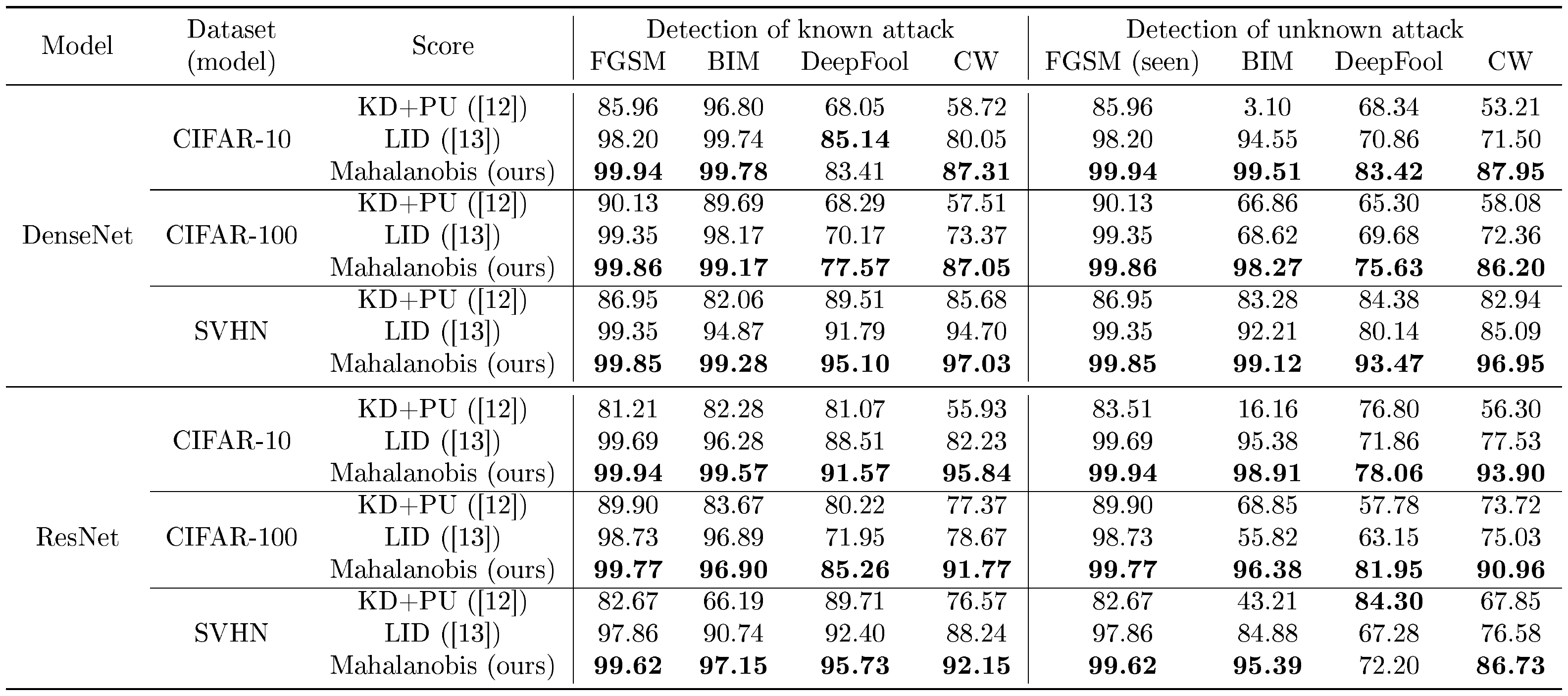
Setup. For the problem of detecting adversarial samples, we train DenseNet and ResNet for classifying CIFAR-10, CIFAR-100 and SVHN datasets, and the corresponding test dataset is used as the positive samples to measure the performance. We use adversarial images as the negative samples generated by the following attack methods: FGSM ([19]), BIM ([20]), DeepFool ([21]) and CW ([22]), where the detailed explanations can be found in the supplementary material. For comparison, we use a logistic regression detector based on combinations of kernel density (KD) ([12]) and predictive uncertainty (PU), i.e., maximum value of posterior distribution. We also compare the state-of-the-art local intrinsic dimensionality (LID) scores ([13]). Following the similar strategies in ([12, 13]), we randomly choose 10% of original test samples for training the logistic regression detectors and the remaining test samples are used for evaluation. Using nested cross-validation within the training set, all hyper-parameters are tuned.

::: {caption="Table 3: Comparison of AUROC (%) under various validation setups. For evaluation on unknown attack, FGSM samples denoted by "seen" are used for validation. For our method, we use both feature ensemble and input pre-processing. The best results are indicated in bold."}

:::

Comparison with LID and generalization analysis. The left-hand column of Table 3 reports the AUROC score of a logistic regression detectors for all normal and adversarial pairs. One can note that the proposed method outperforms all tested methods in most cases. In particular, ours improves the AUROC of LID from $82.2%$ to $95.8%$ when we detect CW samples using ResNet trained on the CIFAR-10 dataset. Similar to ([13]), we also evaluate whether the proposed method is tuned on a simple attack can be generalized to detect other more complex attacks. To this end, we measure the detection performance when we train the logistic regression detector using samples generated by FGSM. As shown in the right-hand column of Table 3, our method trained on FGSM can accurately detect much more complex attacks such as BIM, DeepFool and CW. Even though LID can also generalize well, our method still outperforms it in most cases. A natural question that arises is whether the LID can be useful in detecting OOD samples. We indeed compare the performance of our method with that of LID in the supplementary material, where our method still outperforms LID in all tested case.

3.3 Class-incremental learning

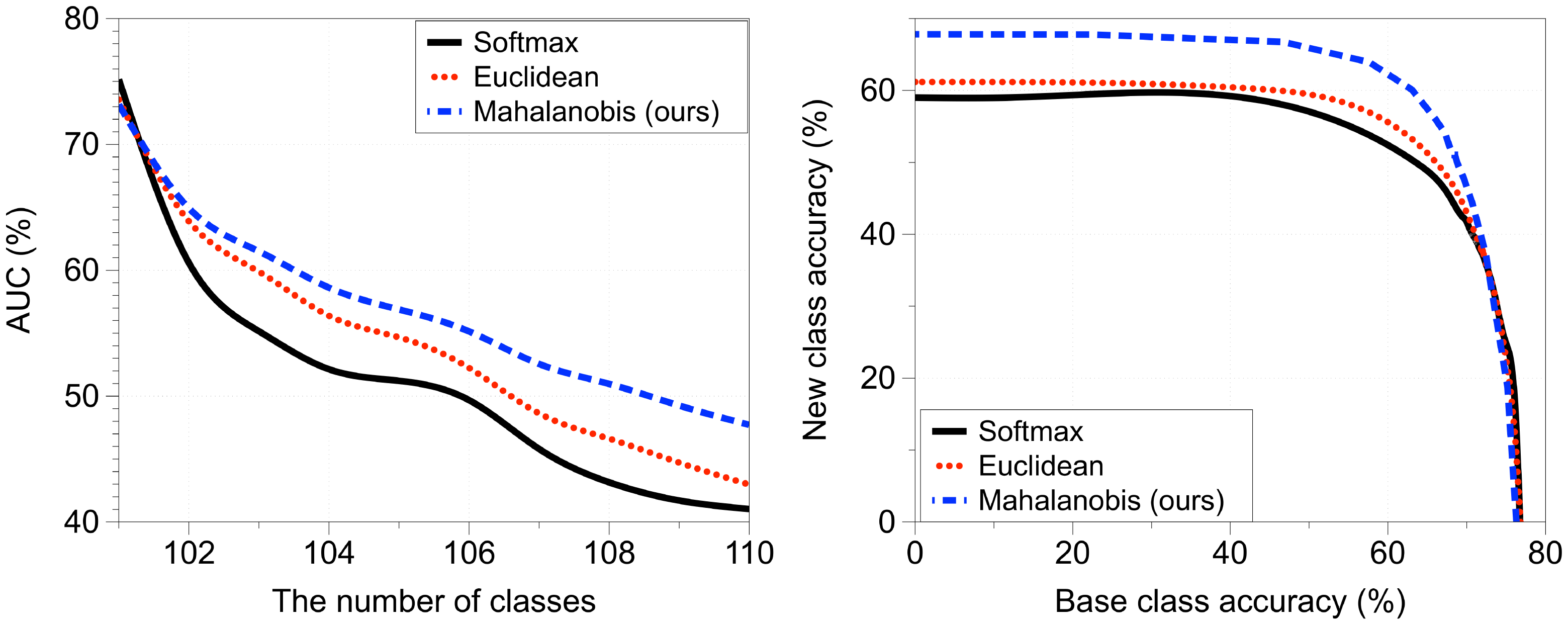
Setup. For the task of class-incremental learning, we train ResNet with 34 layers for classifying CIFAR-100 and downsampled ImageNet ([29]). As described in Section 2.3, we assume that a classifier is pre-trained on a certain amount of base classes and new classes with corresponding datasets are incrementally provided one by one. Specifically, we test two different scenarios: in the first scenario, half of CIFAR-100 classes are bases classes and the rest are new classes. In the second scenario, all classes in CIFAR-100 are considered to be base classes and 100 of ImageNet classes are new classes. All scenarios are tested five times and then averaged. Class splits are randomly generated for each trial. For comparison, we consider a softmax classifier, which is fine-tuned whenever new class data come in, and a Euclidean classifier ([28]), which tries to accommodate a new class by only computing the class mean. For the softmax classifier, we only update the softmax layer to achieve near-zero cost training ([28]), and follow the memory management in [23]: a small number of samples from old classes are kept in the limited memory, where the size of the memory is matched with that for keeping the parameters for Mahalanobis distance-based classifier. Namely, the number of old exemplars kept for training the softmax classifier is chosen as the sum of the number of learned classes and the dimension ($512$ in our experiments) of the hidden features. For evaluation, similar to ([7]), we first draw base-new class accuracy curve by adjusting an additional bias to the new class scores, and measure the area under curve (AUC) since averaging base and new class accuracy may cause an imbalanced measure of the performance between base and new classes.

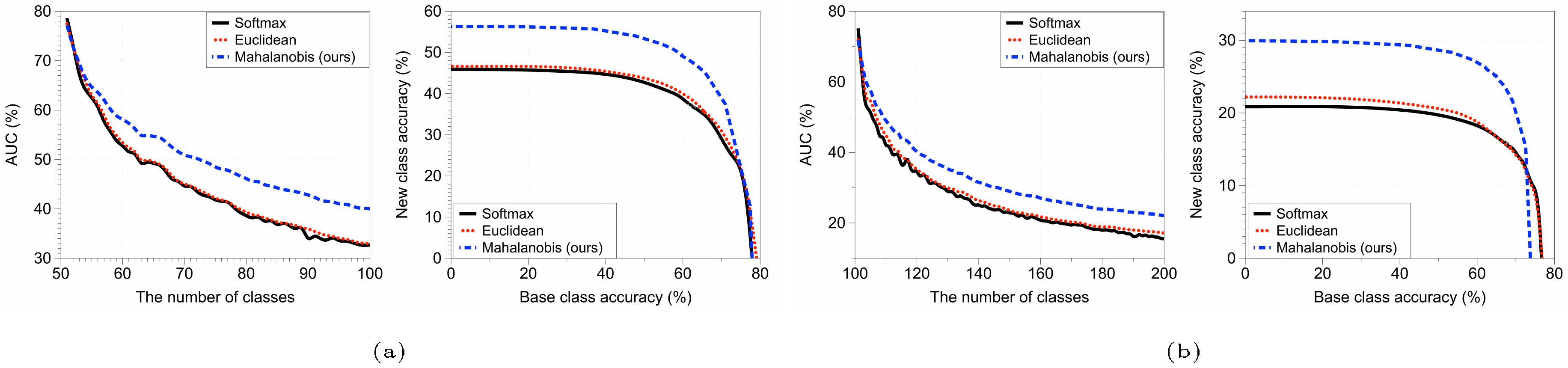
Comparison with other classifiers. Figure 4 compares the incremental learning performance of methods in terms of AUC in the two scenarios mentioned above. In each sub-figure, AUC with respect to the number of learned classes (left) and the base-new class accuracy curve after the last new classes is added (right) are drawn. Our proposed Mahalanobis distance-based classifier outperforms the other methods by a significant margin, as the number of new classes increases, although there is a crossing in the right figure of Figure 4b in small regimes (due to the catastrophic forgetting issue). In particular, the AUC of our proposed method is 40.0% (22.1%), which is better than 32.7% (15.6%) of the softmax classifier and 32.9% (17.1%) of the Euclidean distance classifier after all new classes are added in the first (second) experiment. We also report the experimental results in the supplementary material for the case when classes of CIFAR-100 are base classes and those of CIFAR-10 are new classes, where the overall trend is similar. The experimental results additionally demonstrate the superiority of our confidence score, compared to other plausible ones.

4. Conclusion

Section Summary: This paper introduces a straightforward and powerful technique to spot unusual test samples in machine learning, such as those from unfamiliar data distributions or tampered inputs designed to fool models. The approach involves creating a basic predictive model based on a common statistical assumption and developing a new way to measure confidence in predictions, which, when refined with simple adjustments like data preprocessing and combining features, excels at tasks like identifying out-of-distribution data, countering attacks, and adapting to new classes over time. The method proves reliable even with tricky hyperparameters, imperfect training data, or limited samples, and it holds promise for broader applications in areas like selective data labeling, group model building, and learning from very few examples.

In this paper, we propose a simple yet effective method for detecting abnormal test samples including both out-of-distribution and adversarial ones. In essence, our main idea is inducing a generative classifier under LDA assumption, and defining new confidence score based on it. With calibration techniques such as input pre-processing and feature ensemble, our method performs very strongly across multiple tasks: detecting out-of-distribution samples, detecting adversarial attacks and class-incremental learning. We also found that our proposed method is more robust in the choice of its hyperparameters as well as against extreme scenarios, e.g., when the training dataset has some noisy, random labels or a small number of data samples. We believe that our approach have a potential to apply to many other related machine learning tasks, e.g., active learning ([6]), ensemble learning ([24]) and few-shot learning ([25]).

Acknowledgements

This work was supported in part by Institute for Information & communications Technology Promotion (IITP) grant funded by the Korea government (MSIT) (No.R0132-15-1005, Content visual browsing technology in the online and offline environments), National Research Council of Science & Technology (NST) grant by the Korea government (MSIP) (No. CRC-15-05-ETRI), DARPA Explainable AI (XAI) program #313498, Sloan Research Fellowship, and Kwanjeong Educational Foundation Scholarship.

Appendix

Section Summary: This appendix provides background on classifiers in machine learning, distinguishing between discriminative types that directly map inputs to labels, like softmax models, and generative ones that model data distributions, particularly using Gaussian assumptions in methods like Gaussian Discriminant Analysis and its simplified version, Linear Discriminant Analysis, which can mimic softmax behavior. It then details the experiments for detecting unusual or adversarial inputs, covering the use of advanced neural networks such as DenseNet and ResNet trained on datasets like CIFAR-10 and SVHN, with out-of-distribution tests on images from TinyImageNet and LSUN. The setup also compares baseline confidence scores with techniques like ODIN, which adjusts model outputs via temperature scaling to better identify anomalies.

**Supplementary Material:** **A Simple Unified Framework for Detecting Out-of-Distribution Samples and Adversarial Attacks**

A. Preliminaries for Gaussian discriminant analysis

In this section, we describe the basic concept of the discriminative and generative classifier ([30]). Formally, denote the random variable of the input and label as $\mathbf{x}\in \mathcal{X}$ and $y \in \mathcal{Y} = {1, \cdots, C}$, respectively. For the classification task, the discriminative classifier directly defines a posterior distribution $P(y|\mathbf{x})$, i.e., learning a direct mapping between input $\mathbf{x}$ and label $y$. A popular model for discriminative classifier is softmax classifier which defines the posterior distribution as follows: $P\left(y=c|\mathbf{x}\right) = \frac{ \exp \left(\mathbf{w}c^\top \mathbf{x} + b_c \right) }{\sum{c^\prime} \exp \left(\mathbf{w}{c^\prime}^\top \mathbf{x} + b{c^\prime}\right) }, $ where $\mathbf{w}_c$ and $b_c$ are weights and bias for a class $c$, respectively. In contrast to the discriminative classifier, the generative classifier defines the class conditional distribution $P\left(\mathbf{x}|y\right)$ and class prior $P\left(y \right)$ in order to indirectly define the posterior distribution by specifying the joint distribution $P\left(\mathbf{x}, y\right) = P\left(y \right) P \left(\mathbf{x}| y \right)$. Gaussian discriminant analysis (GDA) is a popular method to define the generative classifier by assuming that the class conditional distribution follows the multivariate Gaussian distribution and the class prior follows Bernoulli distribution: $P\left(\mathbf{x}|y=c\right) = \mathcal{N} \left(\mathbf{x}| \mathbf{\mu}c, \mathbf{\Sigma}c \right), P\left(y=c\right) = \frac{\beta_c}{\sum{c^\prime} \beta{c^\prime}}, $ where $\mathbf{\mu}_c$ and $\mathbf{\Sigma}_c$ are the mean and covariance of multivariate Gaussian distribution, and $\beta_c$ is the unnormalized prior for class $c$. This classifier has been studied in various machine learning areas (e.g., semi-supervised learning ([31]) and incremental learning ([23])).

In this paper, we focus on the special case of GDA, also known as the linear discriminant analysis (LDA). In addition to Gaussian assumption, LDA further assumes that all classes share the same covariance matrix, i.e., $\mathbf{\Sigma}_c = \mathbf{\Sigma}$. Since the quadratic term is canceled out with this assumption, the posterior distribution of generative classifier can be represented as follows:

$ \begin{align*} & P\left(y=c|\mathbf{x}\right) = \frac{P\left(y = c \right) P\left(\mathbf{x}| y =c \right) }{\sum_{c^\prime}P\left(y= c^\prime \right) P\left(\mathbf{x}| y= c^\prime \right)} \notag = \frac{ \exp \left(\mathbf{\mu}c^\top \mathbf{\Sigma}^{-1} \mathbf{x} -\frac{1}{2} \mathbf{\mu}c^\top \mathbf{\Sigma}^{-1} \mathbf{\mu}c +\log \beta_c \right) }{\sum{c^\prime} \exp \left(\mathbf{\mu}{c^\prime}^\top \mathbf{\Sigma}^{-1} \mathbf{x} -\frac{1}{2} \mathbf{\mu}{c^\prime}^\top \mathbf{\Sigma}^{-1} \mathbf{\mu}{c^\prime} +\log \beta{c^\prime} \right)}. \end{align*} $

One can note that the above form of posterior distribution is equivalent to the softmax classifier by considering $\mathbf{\mu}_{c}^\top \mathbf{\Sigma}^{-1}$ and $ -\frac{1}{2} \mathbf{\mu}_c^\top \mathbf{\Sigma}^{-1} \mathbf{\mu}_c +\log \beta_c$ as weight and bias of it, respectively. This implies that $\mathbf{x}$ might be fitted in Gaussian distribution during training a softmax classifier.

B. Experimental setup

In this section, we describe detailed explanation about all the experiments described in Section 3.

B.1 Experimental setups in detecting out-of-distribution

Detailed model architecture and training. We consider two state-of-the-art neural network architectures: DenseNet ([14]) and ResNet ([3]). For DenseNet, our model follows the same setup as in [14]: 100 layers, growth rate $k=12$ and dropout rate 0. Also, we use ResNet with 34 layers and dropout rate 0.[^2] The softmax classifier is used, and each model is trained by minimizing the cross-entropy loss using SGD with Nesterov momentum. Specifically, we train DenseNet for 300 epochs with batch size 64 and momentum 0.9. For ResNet, we train it for 200 epochs with batch size 128 and momentum 0.9. The learning rate starts at 0.1 and is dropped by a factor of 10 at 50% and 75% of the training progress, respectively. The test set errors of DenseNet and ResNet on CIFAR-10, CIFAR-100 and SVHN are reported in Table 4.

[^2]: ResNet architecture is available at https://github.com/kuangliu/pytorch-cifar.

Datasets. We train DenseNet and ResNet for classifying CIFAR-10 (or 100) and SVHN datasets: the former consists of 50, 000 training and 10, 000 test images with 10 (or 100) image classes, and the latter consists of 73, 257 training and 26, 032 test images with 10 digits.[^3] The corresponding test dataset is used as the in-distribution (positive) samples to measure the performance. We use realistic images as the out-of-distribution (negative) samples: the TinyImageNet consists of 10, 000 test images with 200 image classes from a subset of ImageNet images. The LSUN consists of 10, 000 test images of 10 different scenes. We downsample each image of TinyImageNet and LSUN to size $32\times32$.[^4]

[^3]: We do not use the extra SVHN dataset for training.

[^4]: LSUN and TinyImageNet datasets are available at https://github.com/ShiyuLiang/odin-pytorch.

Tested methods. In this paper, we consider the baseline method ([11]) and ODIN ([5]) for comparison. The confidence score in [11] is a maximum value of softmax posterior distribution, i.e., $\max_y P(y|\mathbf{x})$. The key idea of ODIN is the temperature scaling which is defined as follows:

$ \begin{align*} P (y={\widehat{y}}|\mathbf{x};T) = \frac{\exp \left(f_{{\widehat{y}}} (\mathbf{x}) / T \right)}{\sum_{y} \exp \left(f_{ y} (\mathbf{x}) / T \right)}, \end{align*} $

where $T>0$ is the temperature scaling parameter and $\mathbf{f} = (f_1, \ldots, f_K)$ is final feature vector of deep neural networks. For each data $\mathbf{x}$, ODIN first calculates the pre-processed image $\mathbf{\widehat{x}}$ by adding the small perturbations as follows:

$ \begin{align*} \mathbf{x}^\prime = \mathbf{x} - \varepsilon_{odin} \text{sign} \left(-\bigtriangledown_{\mathbf{x}} \log P_{\theta} (y={\widehat{y}}|\mathbf{x};T) \right), \end{align*} $

where $\varepsilon_{odin}$ is a magnitude of noise and $\widehat{y}$ is the predicted label. Next, ODIN feeds the pre-processed data into the classifier, computes the maximum value of scaled predictive distribution, i.e., $\max_y P_{\theta} (y|\mathbf{x}^\prime; T)$, and classifies it as positive (i.e., in-distribution) if the confidence score is above some threshold $\delta$. For ODIN, the perturbation noise $\varepsilon_{odin}$ is chosen from ${0, 0.0005, 0.001, 0.0014, 0.002, 0.0024, 0.005, 0.01, 0.05, 0.1, 0.2 }$, and the temperature $T$ is chosen from ${1, 10, 100, 1000}$.

Hyper parameters for our method. There are two hyper parameters in our method: the magnitude of noise in Equation 4 and layer indexes for feature ensemble. For all experiments, we extract the confidence scores from every end of dense (or residual) block of DenseNet (or ResNet). The size of feature maps on each convolutional layers is reduced by average pooling for computational efficiency: $\mathcal{F} \times \mathcal{H} \times \mathcal{W} \rightarrow \mathcal{F} \times 1$, where $\mathcal{F}$ is the number of channels and $\mathcal{H} \times \mathcal{W}$ is the spatial dimension. The magnitude of noise in Equation 4 is chosen from ${0, 0.0005, 0.001, 0.0014, 0.002, 0.0024, 0.005, 0.01, 0.05, 0.1, 0.2 }$.

Performance metrics. For evaluation, we measure the following metrics to measure the effectiveness of the confidence scores in distinguishing in- and out-of-distribution images.

• True negative rate (TNR) at 95% true positive rate (TPR). Let TP, TN, FP, and FN denote true positive, true negative, false positive and false negative, respectively. We measure TNR = TN / (FP+TN), when TPR = TP / (TP+FN) is 95%.
• Area under the receiver operating characteristic curve (AUROC). The ROC curve is a graph plotting TPR against the false positive rate = FP / (FP+TN) by varying a threshold.
• Area under the precision-recall curve (AUPR). The PR curve is a graph plotting the precision = TP / (TP+FP) against recall = TP / (TP+FN) by varying a threshold. AUPR-IN (or -OUT) is AUPR where in- (or out-of-) distribution samples are specified as positive.
• Detection accuracy. This metric corresponds to the maximum classification probability over all possible thresholds $\delta$:

$ \begin{align*} 1- \min_{\delta} \big{ P_{\texttt{in}} \left(q \left(\mathbf{x} \right) \leq \delta \right) P \left(\mathbf{x}\text{ is from }P_{\texttt{in}}\right)+ P_{\texttt{out}} \left(q \left(\mathbf{x} \right) >\delta \right) P \left(\mathbf{x}\text{ is from }P_{\texttt{out}}\right)\big}, \end{align*} $

where $q(\mathbf{x})$ is a confident score.

We assume that both positive and negative examples have equal probability of appearing in the test set, i.e., $P \left(\mathbf{x}\text{ is from }P_{\texttt{in}}\right) = P \left(\mathbf{x}\text{ is from }P_{\texttt{out}}\right)$.

Note that AUROC, AUPR and detection accuracy are threshold-independent evaluation metrics.

B.2 Experimental setups in detecting adversarial samples

Adversarial attacks. For the problem of detecting adversarial samples, we consider the following attack methods: fast gradient sign method (FGSM) ([19]), basic iterative method (BIM) ([20]), DeepFool ([21]) and Carlini-Wagner (CW) ([22]). The FGSM directly perturbs normal input in the direction of the loss gradient. Formally, non-targeted adversarial examples are constructed as

$ \begin{align*} \mathbf{x}{adv} = \mathbf{x} + \varepsilon{FGSM} \text{sign} \left(\bigtriangledown_{\mathbf{x}} \ell (y^*, P(y|\mathbf{x})) \right), \end{align*} $

where $\varepsilon_{FGSM}$ is a magnitude of noise, $y^*$ is the ground truth label and $\ell$ is a loss function to measure the distance between the prediction and the ground truth. The BIM is an iterative version of FGSM, which applies FGSM multiple times with a smaller step size. Formally, non-targeted adversarial examples are constructed as

$ \begin{align*} \mathbf{x}{adv}^0 = \mathbf{x}, ~ \mathbf{x}{adv}^{n+1} = \text{Clip}^{\varepsilon_{BIM}}{\mathbf{x}} { \mathbf{x}{adv}^{n} + \alpha_{BIM} \text{sign} \left(\bigtriangledown_{\mathbf{x}{adv}^{n}} \ell (y^*, P(y|{\mathbf{x}{adv}^{n}})) \right)}, \end{align*} $

where $\text{Clip}{\mathbf{x}}^{\varepsilon{BIM}}$ means we clip the resulting image to be within the $\varepsilon_{BIM}$-ball of $\mathbf{x}$. DeepFool works by finding the closest adversarial examples with geometric formulas. CW is an optimization-based method which arguably the most effective method. Formally, non-targeted adversarial examples are constructed as

$ \begin{align*} \arg \min_{\mathbf{x}{adv}} ; \lambda d(\mathbf{x}, \mathbf{x}{adv}) - \ell(y^*, P(y|\mathbf{x}_{adv})), \end{align*} $

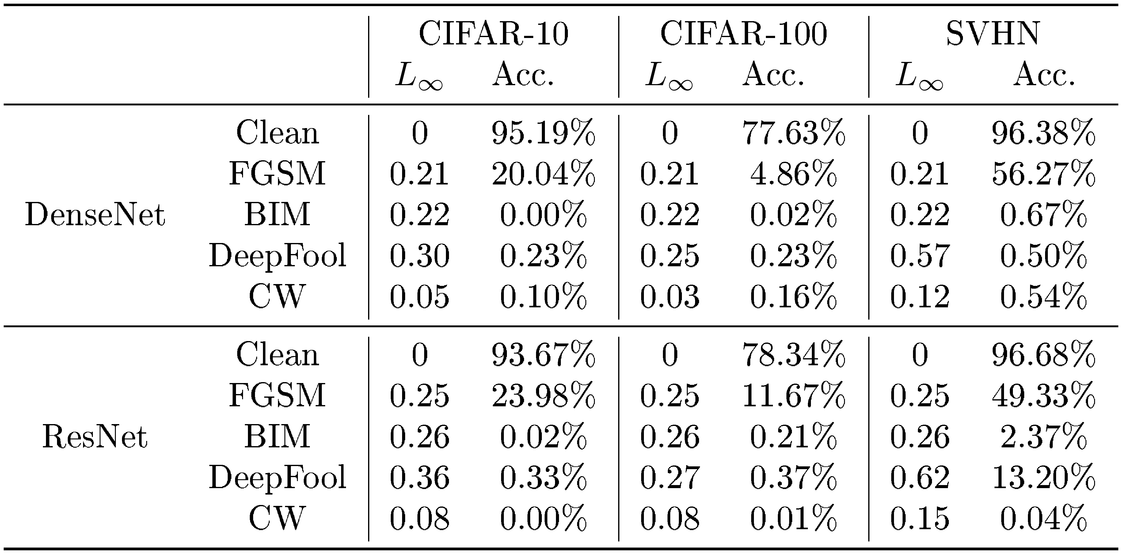
where $\lambda$ is penalty parameter and $d(\cdot, \cdot)$ is a metric to quantify the distance between an original image and its adversarial counterpart. However, compared to FGSM and BIM, this method is much slower in practice. For all experiments, $L_2$ distance is used as a constraint. We used the library from FaceBook ([32]) for generating adversarial samples.[^5] Table 4 tatistics of adversarial attacks including the $L_{\infty}$ mean perturbation and classification accuracy on adversarial attacks.

[^5]: The code is available at https://github.com/facebookresearch/adversarial_image_defenses.

::: {caption="Table 4: The $L_{\infty}$ mean perturbation and classification accuracy on clean and adversarial samples."}

:::

Tested methods. [13] proposed to characterize adversarial subspaces by using local intrinsic dimensionality (LID). Given a test sample $\mathbf{x}$, LID is defined as follows:

$ \begin{align*} {\widehat{L}ID} = - \left(\frac{1}{k} \sum_i \log \frac{r_i(\mathbf{x})}{r_k(\mathbf{x})} \right), \end{align*} $

where $r_i(\mathbf{x})$ denotes the distance between $\mathbf{x}$ and its $i$-th nearest neighbor within a sample of points drawn from in-distribution, and $r_k(\mathbf{x})$ denotes the maximum distance among $k$ nearest neighbors. We commonly extract the LID scores from every end of dense (or residual) block of DenseNet (or ResNet) similar to ours. Given test sample $\mathbf{x}$ and the set $\mathbf{X}_c$ of training samples with label $c$, the Gaussian kernel density with bandwidth $\sigma$ is defined as follows:

$ \begin{align*} KD(\mathbf{x}) = \frac{1}{|\mathbf{X}c|} \sum{\mathbf{x}_i \in \mathbf{X}c} k{\sigma}(\mathbf{x}_i, \mathbf{x}), \end{align*} $

where $k_{\sigma}(x, y) \propto \exp(-||x-y||^2/\sigma^2)$. For LID and KD, we used the library from [13].

Hyper-parameters and training. Following the similar strategies in ([12, 13]), we randomly choose 10% of original test samples for training the logistic regression detectors and the remaining test samples are used for evaluation. The training sets consists of three types of examples: adversarial, normal and noisy. Here, noisy examples are generated by adding random noise to normal examples. Using nested cross validation within the training set, all hyper-parameters including the bandwidth parameter for KD, the number of nearest neighbors for LID, and input noise for our method are tuned. Specifically, the value of $k$ is chosen from ${10, 20, 30, 40, 50, 60, 70, 80, 90}$ with respect to a minibatch of size 100, and the bandwidth was chosen from ${0.1, 0.25, 0.5, 0.75, 1}$. The magnitude of noise in Equation 4 is chosen from ${0, 0.0005, 0.001, 0.0014, 0.002, 0.0024, 0.005, 0.01, 0.05, 0.1, 0.2 }$.

C. More experimental results

In this section, we provide more experimental results.

C.1 Robustness of our method in detecting adversarial samples

In order to verify the robustness, we measure the detection performance when we train ResNet by varying the number of training data and assigning random label to training data on CIFAR-10 dataset. As shown in Figure 5, our method (blue bar) outperforms LID (green bar) for all experiments.

C.2 Class-incremental learning

Figure 6 compares the AUCs of tested methods when CIFAR-100 is pre-trained and CIFAR-10 is used as new classes. Our proposed Mahalanobis distance-based classifier outperforms the other methods by a significant margin, as the number of new classes increases. The AUC of our proposed method is 47.7%, which is better than 41.0% of the softmax classifier and 43.0% of the Euclidean distance classifier after all new classes are added.

C.3 Experimental results on joint confidence loss

In addition, we remark that the proposed detector using softmax neural classifier trained by standard cross entropy loss typically outperforms the ODIN detector using softmax neural classifier trained by confidence loss ([24]) which involves jointly training a generator and a classifier to calibrate the posterior distribution. Also, our detector provides further improvement if one use it with model trained by confidence loss. In other words, our proposed method can improve any pre-trained softmax neural classifier.

::: {caption="Table 5: Distinguishing in- and out-of-distribution test set data for image classification. We tune the hyper-parameters using validation set of in- and out-of-distributions. All values are percentages and the best results are indicated in bold."}

:::

::: {caption="Table 6: Distinguishing in- and out-of-distribution test set data for image classification when we tune the hyper-parameters of ODIN and our method only using in-distribution and adversarial (FGSM) samples. All values are percentages and boldface values indicate relative the better results."}

:::

C.4 LID for detecting out-of-distribution samples

Figure 8 and Figure 9 shows the performance of the ODIN ([5]), LID ([13]) and Mahalanobis detector for each in- and out-of-distribution pair. We remark that the proposed method outperforms all tested methods.

D. Evaluation on ImageNet dataset

In this section, we verify the performance of the proposed method using the ImageNet 2012 classification dataset ([17]) that consists of 1000 classes. The models are trained on the 1.28 million training images, and evaluated on the 50k validation images. For all experiments, we use the pre-trained ResNet ([3]) which is available at https://github.com/pytorch/vision/blob/master/torchvision/models/resnet.py. First, we measure the classification accuracy of generative classifier from the pre-trained model as follows:

$ \begin{align*} \widehat{y} (\mathbf{x}) = \arg \min_c \left(f(\mathbf{x}) - {\widehat{\mu}}{c} \right)^\top \mathbf{\widehat{\Sigma}}^{-1} \left(f(\mathbf{x}) - {\widehat{\mu}}{c}\right) + \log {\widehat{\beta}}_c, \end{align*} $

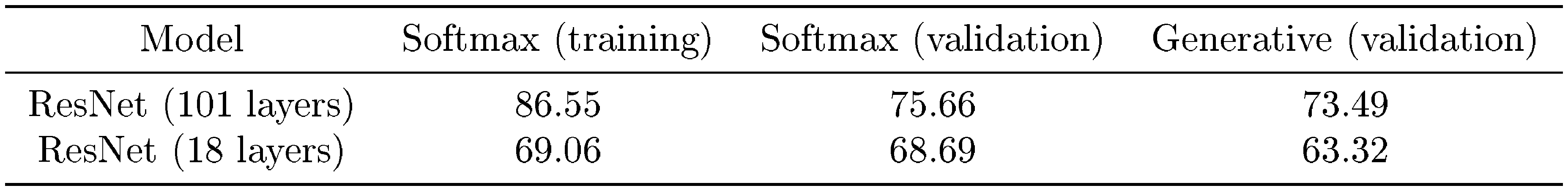
where ${\widehat{\beta}}_c = \frac{N_c}{N}$ is an empirical class prior. We remark that this corresponds to predicting a class label using the posterior distribution from generative with LDA assumption. Table 7 shows the top-1 classification accuracy on ImageNet 2012 dataset. One can note that the proposed generative classifier can perform reasonably well even though the softmax classifier outperforms it in all cases. However, we remark that the gap between them is decreasing as the training accuracy increases, i.e., the pre-trained model learned more strong representations.

::: {caption="Table 7: Top-1 accuracy (%) of ResNets on ImageNet 2012 dataset."}

:::

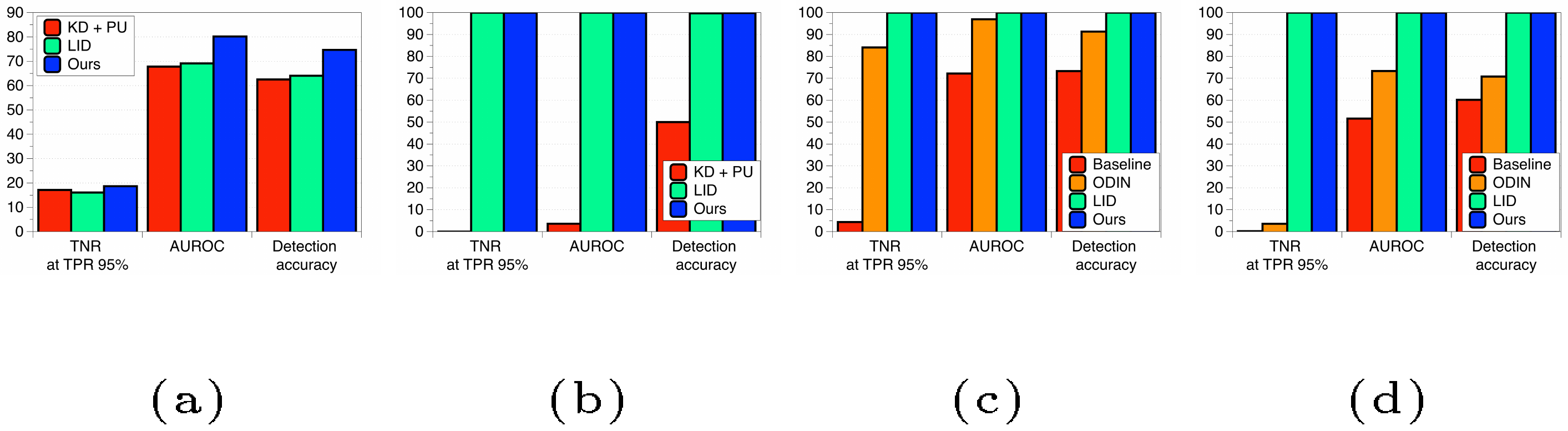
Next, we also evaluate the detection performance of the Mahalanobis distance-based detector on ImageNet 2012 dataset using ResNets with 18 layers. For evaluation, we consider the problem of detecting adversarial samples generated by FGSM ([19]) and BIM ([20]). Similar to Section 3.2, we extract the confidence scores from every end of residual block of ResNet. Figure 10a and Figure 10b show the performance of various detectors. One can note that the proposed Mahalanobis distance-based detector outperforms all tested methods including LID. These results imply that our method can be working well for the large-scale datasets.

E. Adaptive attacks against Mahalanobis distance-based detector

In this section, we evaluate the robustness of our method by generating the garbage images which may fool the Mahalanobis distance-based detector in a white-box setting, i.e., one can access to the parameters of the classifier and that of the Mahalanobis distance-based detector. Here, we remark that accessing the parameters of the Mahalanobis distance-based detector, i.e., sample means and covariance, is not mild assumption since the information about training data is required to compute them. To attack our method, we generate a garbage images $\mathbf{x}_{g}$ by minimizing the Mahalanobis distance as follows:

$ \begin{align*} \arg \min_{\mathbf{x}{g}} \left(f(\mathbf{x}{g}) - {\widehat{\mu}}{c}\right)^\top \mathbf{\widehat{\Sigma}}^{-1} \left(f(\mathbf{x}{g}) - {\widehat{\mu}}_{c}\right), \end{align*} $

where $c$ is a target class. We test two different scenarios using ResNet with 34 layers trained on CIFAR-10 dataset. In the first scenario, we generate the garbage images only using a penultimate layer of DNNs. In the second scenario, we attack every end of residual block of ResNet. Figure 11 shows the generated samples by minimizing the Mahalanobis distance. Even though the generated sample looks like the random noise, it successfully fools the pre-trained classifier, i.e., it is classified as the target class. We measure the detection performance of the baseline ([11]), ODIN ([5]), LID ([13]) and the proposed Mahalanobis distance-based detector. As shown in Figure 10c and Figure 10d, our method can distinguish CIFAR-10 test and garbage images for both scenarios better than the tested methods. In particular, we remark that the input pre-processing is very useful in detecting such garbage samples. These results imply that our proposed method is robust to the attacks.

F. Hybrid inference of generative and discriminative classifiers

In this paper, we show that the generative classifier can be very useful in characterizing the abnormal samples such as OOD and adversarial samples. Here, a caveat is that the generative classifier might degrade the classification performance. In order to handle this issue, we introduce a hybrid inference of generative and discriminative classifiers. Given a generative classifier with GDA assumptions, the posterior distribution of generative classifier via Bayes rule is given as:

$ \begin{align*} & P\left(y=c|\mathbf{x}\right) = \frac{P\left(y = c \right) P\left(\mathbf{x}| y =c \right) }{\sum_{c^\prime}P\left(y= c^\prime \right) P\left(\mathbf{x}| y= c^\prime \right)} \notag = \frac{ \exp \left(\mathbf{\mu}c^\top \mathbf{\Sigma}^{-1} \mathbf{x} -\frac{1}{2} \mathbf{\mu}c^\top \mathbf{\Sigma}^{-1} \mathbf{\mu}c +\log \beta_c \right) }{\sum{c^\prime} \exp \left(\mathbf{\mu}{c^\prime}^\top \mathbf{\Sigma}^{-1} \mathbf{x} -\frac{1}{2} \mathbf{\mu}{c^\prime}^\top \mathbf{\Sigma}^{-1} \mathbf{\mu}{c^\prime} +\log \beta{c^\prime} \right)}. \end{align*} $

To match this with a standard softmax classifier's weights, the parameters of the generative classifier have to satisfy the following conditions:

$ \begin{align*} \mu_c = \Sigma \mathbf{w}_c, ~\log \beta_c - 0.5 \mu_c^\top \Sigma^{-1}\mu_c = b_c, \end{align*} $

where $\mathbf{w}_c$ and $b_c$ are weights and bias for a class $c$, respectively. Using the empirical covariance ${\widehat{\Sigma}}$ as shown in Equation 1, one can induce the parameters of another generative classifier which has same decision boundary with the softmax classifier as follows:

$ \begin{align*} {\tilde{\mu}}_c = {\widehat{\Sigma}} \mathbf{w}c, {\tilde{\beta}}c = \frac{\exp(0.5 {\tilde{\mu}}c^\top {\widehat{\Sigma}}^{-1}{\tilde{\mu}}c - b_c)}{\sum{c^\prime}\exp(0.5 {\tilde{\mu}}{c^\prime}^\top {\widehat{\Sigma}}^{-1}{\tilde{\mu}}{c^\prime} - b{c^\prime})}. \end{align*} $

Here, we normalize the ${\tilde{\beta}}_c$ to satisfy $\sum_c {\tilde{\beta}}_c = 1$. Then, using this generative classifier, we define new hybrid posterior distribution which combines the softmax- and sample-based generative classifiers:

$ \begin{align*} & P_{h}(y|\mathbf{x}) \ & = \frac{\exp \left(\lambda \left(\mathbf{\widehat{\mu}}_c^\top \mathbf{ \widehat{\Sigma}}^{-1} \mathbf{x} -0.5 \mathbf{\widehat{\mu}}_c^\top \mathbf{\widehat{\Sigma}}^{-1} \mathbf{\widehat{\mu}}_c +\log {\widehat{\beta}}_c \right)

• (1-\lambda) \left(\mathbf{\tilde{\mu}}c^\top \mathbf{ \widehat{\Sigma}}^{-1} \mathbf{x} -0.5 \mathbf{\tilde{\mu}}c^\top \mathbf{\widehat{\Sigma}}^{-1} \mathbf{\tilde{\mu}}c +\log {\tilde{\beta}}c \right)\right)}{\sum{c^\prime} \exp \left(\lambda \left(\mathbf{\widehat{\mu}}{c^\prime}^\top \mathbf{ \widehat{\Sigma}}^{-1} \mathbf{x} -0.5 \mathbf{\widehat{\mu}}{c^\prime}^\top \mathbf{\widehat{\Sigma}}^{-1} \mathbf{\widehat{\mu}}{c^\prime} +\log {\widehat{\beta}}_{c^\prime} \right)
• (1-\lambda) \left(\mathbf{\tilde{\mu}}{c^\prime}^\top \mathbf{ \widehat{\Sigma}}^{-1} \mathbf{x} -0.5 \mathbf{\tilde{\mu}}{c^\prime}^\top \mathbf{\widehat{\Sigma}}^{-1} \mathbf{\tilde{\mu}}{c^\prime} +\log {\tilde{\beta}}{c^\prime} \right)\right)}, \end{align*} $

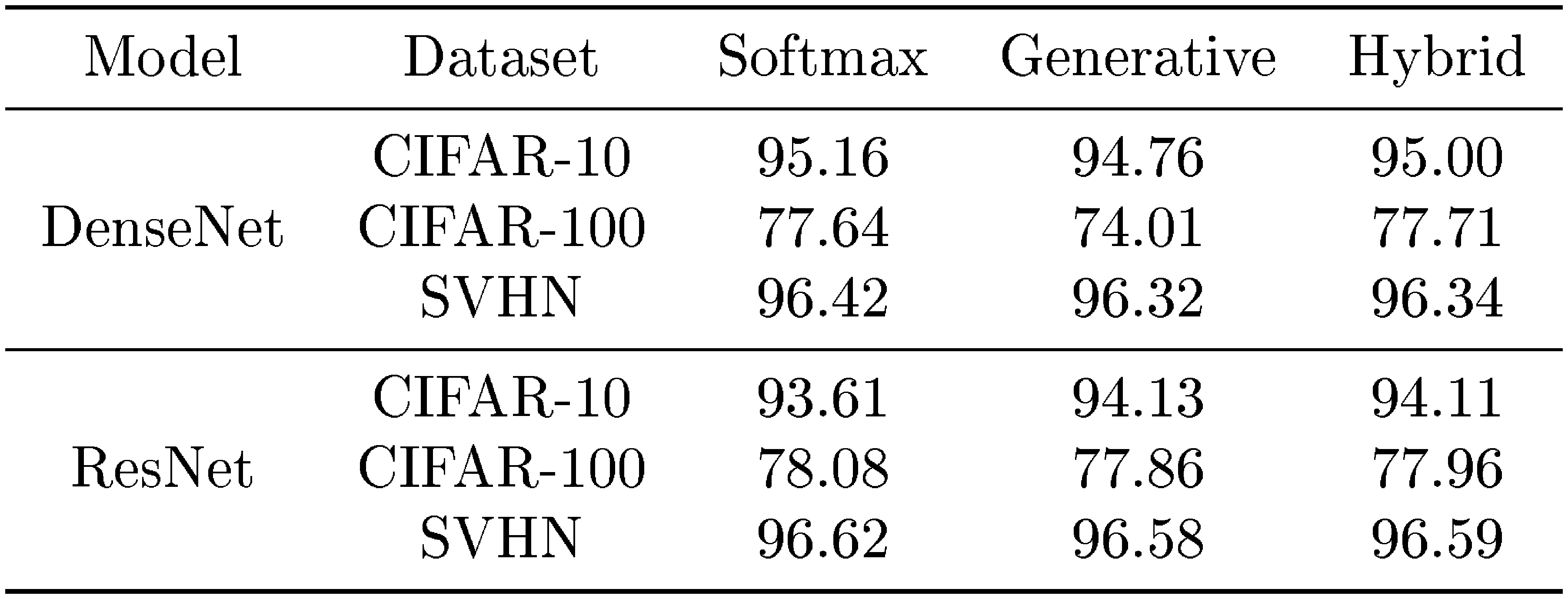
where $\lambda \in [0, 1]$ is a hyper-parameter. This hybrid model can be interpreted as ensemble of softmax and generative classifiers, and one can expect that it can improve the classification performance. Table 8 compares the classification accuracy of softmax, generative and hybrid classifiers. One can note that the hybrid model improves the classification accuracy, where we determine the optimal tuning parameter between the two objectives using the validation set. We also remark that such hybrid model can be useful in detecting the abnormal samples, where we pursue these tasks in the future.

::: {caption="Table 8: Classification test set accuracy (%) of DenseNet and ResNet on CIFAR-10, CIFAR-100 and SVHN datasets."}

:::

References

[1] Amodei, Dario, Ananthanarayanan, Sundaram, Anubhai, Rishita, Bai, Jingliang, Battenberg, Eric, Case, Carl, Casper, Jared, Catanzaro, Bryan, Cheng, Qiang, Chen, Guoliang, et al. Deep speech 2: End-to-end speech recognition in english and mandarin. In ICML, 2016a.

[2] Girshick, Ross. Fast r-cnn. In ICCV, 2015.

[3] He, Kaiming, Zhang, Xiangyu, Ren, Shaoqing, and Sun, Jian. Deep residual learning for image recognition. In CVPR, 2016.

[4] Lee, Kimin, Lee, Honglak, Lee, Kibok, and Shin, Jinwoo. Training confidence-calibrated classifiers for detecting out-of-distribution samples. In ICLR, 2018b.

[5] Liang, Shiyu, Li, Yixuan, and Srikant, R. Principled detection of out-of-distribution examples in neural networks. In ICLR, 2018.

[6] Gal, Yarin, Islam, Riashat, and Ghahramani, Zoubin. Deep bayesian active learning with image data. In ICML, 2017.

[7] Lee, Kibok, Lee, Kimin, Min, Kyle, Zhang, Yuting, Shin, Jinwoo, and Lee, Honglak. Hierarchical novelty detection for visual object recognition. In CVPR, 2018a.

[8] Amodei, Dario, Olah, Chris, Steinhardt, Jacob, Christiano, Paul, Schulman, John, and Mané, Dan. Concrete problems in ai safety. arXiv preprint arXiv:1606.06565, 2016b.

[9] Evtimov, Ivan, Eykholt, Kevin, Fernandes, Earlence, Kohno, Tadayoshi, Li, Bo, Prakash, Atul, Rahmati, Amir, and Song, Dawn. Robust physical-world attacks on machine learning models. In CVPR, 2018.

[10] Sharif, Mahmood, Bhagavatula, Sruti, Bauer, Lujo, and Reiter, Michael K. Accessorize to a crime: Real and stealthy attacks on state-of-the-art face recognition. In ACM SIGSAC, 2016.

[11] Hendrycks, Dan and Gimpel, Kevin. A baseline for detecting misclassified and out-of-distribution examples in neural networks. In ICLR, 2017.

[12] Feinman, Reuben, Curtin, Ryan R, Shintre, Saurabh, and Gardner, Andrew B. Detecting adversarial samples from artifacts. arXiv preprint arXiv:1703.00410, 2017.

[13] Ma, Xingjun, Li, Bo, Wang, Yisen, Erfani, Sarah M, Wijewickrema, Sudanthi, Houle, Michael E, Schoenebeck, Grant, Song, Dawn, and Bailey, James. Characterizing adversarial subspaces using local intrinsic dimensionality. In ICLR, 2018.

[14] Huang, Gao and Liu, Zhuang. Densely connected convolutional networks. In CVPR, 2017.

[15] Krizhevsky, Alex and Hinton, Geoffrey. Learning multiple layers of features from tiny images. 2009.

[16] Netzer, Yuval, Wang, Tao, Coates, Adam, Bissacco, Alessandro, Wu, Bo, and Ng, Andrew Y. Reading digits in natural images with unsupervised feature learning. In NIPS workshop, 2011.

[17] Deng, Jia, Dong, Wei, Socher, Richard, Li, Li-Jia, Li, Kai, and Fei-Fei, Li. Imagenet: A large-scale hierarchical image database. In CVPR, 2009.

[18] Yu, Fisher, Seff, Ari, Zhang, Yinda, Song, Shuran, Funkhouser, Thomas, and Xiao, Jianxiong. Lsun: Construction of a large-scale image dataset using deep learning with humans in the loop. arXiv preprint arXiv:1506.03365, 2015.

[19] Goodfellow, Ian J, Shlens, Jonathon, and Szegedy, Christian. Explaining and harnessing adversarial examples. In ICLR, 2015.

[20] Kurakin, Alexey, Goodfellow, Ian, and Bengio, Samy. Adversarial examples in the physical world. arXiv preprint arXiv:1607.02533, 2016.

[21] Moosavi Dezfooli, Seyed Mohsen, Fawzi, Alhussein, and Frossard, Pascal. Deepfool: a simple and accurate method to fool deep neural networks. In CVPR, 2016.

[22] Carlini, Nicholas and Wagner, David. Adversarial examples are not easily detected: Bypassing ten detection methods. In ACM workshop on AISec, 2017.

[23] Rebuffi, Sylvestre-Alvise and Kolesnikov, Alexander. icarl: Incremental classifier and representation learning. In CVPR, 2017.

[24] Lee, Kimin, Hwang, Changho, Park, KyoungSoo, and Shin, Jinwoo. Confident multiple choice learning. In ICML, 2017.

[25] Vinyals, Oriol, Blundell, Charles, Lillicrap, Tim, Wierstra, Daan, et al. Matching networks for one shot learning. In NIPS, 2016.

[26] Maaten, Laurens van der and Hinton, Geoffrey. Visualizing data using t-sne. Journal of machine learning research, 2008.

[27] McCloskey, Michael and Cohen, Neal J. Catastrophic interference in connectionist networks: The sequential learning problem. In Psychology of learning and motivation. Elsevier, 1989.

[28] Mensink, Thomas, Verbeek, Jakob, Perronnin, Florent, and Csurka, Gabriela. Distance-based image classification: Generalizing to new classes at near-zero cost. IEEE transactions on pattern analysis and machine intelligence, 2013.

[29] Chrabaszcz, Patryk, Loshchilov, Ilya, and Hutter, Frank. A downsampled variant of imagenet as an alternative to the cifar datasets. arXiv preprint arXiv:1707.08819, 2017.

[30] Murphy, Kevin P. Machine learning: a probabilistic perspective. 2012.

[31] Lasserre, Julia A, Bishop, Christopher M, and Minka, Thomas P. Principled hybrids of generative and discriminative models. In CVPR, 2006.

[32] Guo, Chuan, Rana, Mayank, Cissé, Moustapha, and van der Maaten, Laurens. Countering adversarial images using input transformations. arXiv preprint arXiv:1711.00117, 2017.