1) Purpose
Diffusion models create high-quality images, audio, and video but require many steps, making generation slow. This work develops consistency models to enable fast one-step generation while keeping high quality and editing abilities.
2) Approach
Researchers built models that map noisy data at any time step directly to clean data along a diffusion trajectory. They enforce outputs to match for points on the same path. Training uses two ways: distilling from existing diffusion models (consistency distillation) or training alone (consistency training). Sampling starts from noise and runs one or more model steps.
3) Key methods
- Consistency distillation: Pairs nearby trajectory points using a diffusion model's solver; trains by matching model predictions on pairs.
- Consistency training: Samples noise directly; matches predictions without a diffusion model.
Both use image similarity metrics like LPIPS and support multi-step refinement or editing like inpainting.
4) Main findings
Consistency distillation set records: 3.55 FID (image quality score, lower better) on CIFAR-10 and 6.20 on ImageNet 64x64 for one step, beating prior distillation methods. Standalone training beat non-adversarial one-step generators on CIFAR-10 (8.70 FID). Models support editing tasks like colorization and super-resolution without task-specific training. Multi-step sampling traded steps for better quality.
5) Implications
One-step generation cuts compute 10-2000 times versus diffusion models, enabling real-time use and reducing costs. Editing boosts applications in design and medicine without retraining. Standalone training removes reliance on diffusion models, speeding development. Outperforms some GANs without adversarial training risks like instability.
6) Recommendations and next steps
Adopt consistency distillation for fastest high-quality generation from existing diffusion models. Use standalone training for new setups without diffusion dependencies. Test multi-step sampling (2-4 steps) for production quality gains. Explore audio/video; run pilots on custom data. Trade-off: distillation needs pre-trained models but trains faster.
7) Limitations and confidence
Tested only on images up to 256x256; audio/video unproven. Relies on diffusion setups like VP-SDE. Continuous-time training variants need better frameworks. High confidence in image results (multiple datasets, baselines beaten); caution on scaling to video or unseen domains needs more data.
Yang Song 1{}^{1}1
Prafulla Dhariwal 1{}^{1}1
Mark Chen 1{}^{1}1
Ilya Sutskever 1{}^{1}1
1{}^{1}1 OpenAI, San Francisco, CA 94110, USA. Correspondence to: Yang Song [email protected].
Proceedings of the 40th40^{th}40th International Conference on Machine Learning, Honolulu, Hawaii, USA. PMLR 202, 2023. Copyright 2023 by the author(s).
1{}^{1}1 OpenAI, San Francisco, CA 94110, USA. Correspondence to: Yang Song [email protected].
Proceedings of the 40th40^{th}40th International Conference on Machine Learning, Honolulu, Hawaii, USA. PMLR 202, 2023. Copyright 2023 by the author(s).
Abstract
Diffusion models have significantly advanced the fields of image, audio, and video generation, but they depend on an iterative sampling process that causes slow generation. To overcome this limitation, we propose consistency models, a new family of models that generate high quality samples by directly mapping noise to data. They support fast one-step generation by design, while still allowing multistep sampling to trade compute for sample quality. They also support zero-shot data editing, such as image inpainting, colorization, and super-resolution, without requiring explicit training on these tasks. Consistency models can be trained either by distilling pre-trained diffusion models, or as standalone generative models altogether. Through extensive experiments, we demonstrate that they outperform existing distillation techniques for diffusion models in one- and few-step sampling, achieving the new state-of-the-art FID of 3.55 on CIFAR-10 and 6.20 on ImageNet 64×6464\times 6464×64 for one-step generation. When trained in isolation, consistency models become a new family of generative models that can outperform existing one-step, non-adversarial generative models on standard benchmarks such as CIFAR-10, ImageNet 64×6464\times 6464×64 and LSUN 256×256256\times 256256×256.
1. Introduction
Show me a brief summary.
In this section, diffusion models excel in generating images, audio, and video but suffer from slow iterative sampling requiring excessive compute. Consistency models address this by learning to map any noisy point along a probability flow ODE trajectory directly to clean data origins, enforcing self-consistency where trajectory points yield identical outputs. This enables one-step generation from noise while supporting multistep sampling for quality gains and zero-shot editing like inpainting or super-resolution, trained via distillation from diffusion models or standalone without adversarial objectives. They achieve state-of-the-art FID scores of 3.55 (one-step) and 2.93 (two-step) on CIFAR-10, 6.20 and 4.70 on ImageNet 64×64, outperforming distillation methods, GANs, and non-adversarial one-step generators across benchmarks.
Failed to load: **Figure 1:** Given a Probability Flow (PF) ODE that smoothly converts data to noise, we learn to map any point (*e.g*, ${\mathbf{x}}_t$, ${\mathbf{x}}_{t'}$, and ${\mathbf{x}}_T$) on the ODE trajectory to its origin (*e.g*, ${\mathbf{x}}_0$) for generative modeling. Models of these mappings are called consistency models, as their outputs are trained to be consistent for points on the same trajectory.
Figure 1: Given a Probability Flow (PF) ODE that smoothly converts data to noise, we learn to map any point (e.g, xt, xt′, and xT) on the ODE trajectory to its origin (e.g, x0) for generative modeling. Models of these mappings are called consistency models, as their outputs are trained to be consistent for points on the same trajectory.
💭 Click to ask about this figure
Diffusion models [1, 2, 3, 4, 5], also known as score-based generative models, have achieved unprecedented success across multiple fields, including image generation [6, 7, 8, 9, 10], audio synthesis [11, 12, 13], and video generation [14, 15]. A key feature of diffusion models is the iterative sampling process which progressively removes noise from random initial vectors. This iterative process provides a flexible trade-off of compute and sample quality, as using extra compute for more iterations usually yields samples of better quality. It is also the crux of many zero-shot data editing capabilities of diffusion models, enabling them to solve challenging inverse problems ranging from image inpainting, colorization, stroke-guided image editing, to Computed Tomography and Magnetic Resonance Imaging [2, 5, 16, 17, 18, 19, 20, 21]. However, compared to single-step generative models like GANs [22], VAEs [23, 24], or normalizing flows [25, 26, 27], the iterative generation procedure of diffusion models typically requires 10–2000 times more compute for sample generation [3, 4, 5, 28, 29], causing slow inference and limited real-time applications.
Our objective is to create generative models that facilitate efficient, single-step generation without sacrificing important advantages of iterative sampling, such as trading compute for sample quality when necessary, as well as performing zero-shot data editing tasks. As illustrated in Figure 1, we build on top of the probability flow (PF) ordinary differential equation (ODE) in continuous-time diffusion models [5], whose trajectories smoothly transition the data distribution into a tractable noise distribution. We propose to learn a model that maps any point at any time step to the trajectory's starting point. A notable property of our model is self-consistency: points on the same trajectory map to the same initial point. We therefore refer to such models as consistency models. Consistency models allow us to generate data samples (initial points of ODE trajectories, e.g, x0{\mathbf{x}}_0x0 in Figure 1) by converting random noise vectors (endpoints of ODE trajectories, e.g, xT{\mathbf{x}}_TxT in Figure 1) with only one network evaluation. Importantly, by chaining the outputs of consistency models at multiple time steps, we can improve sample quality and perform zero-shot data editing at the cost of more compute, similar to what iterative sampling enables for diffusion models.
To train a consistency model, we offer two methods based on enforcing the self-consistency property. The first method relies on using numerical ODE solvers and a pre-trained diffusion model to generate pairs of adjacent points on a PF ODE trajectory. By minimizing the difference between model outputs for these pairs, we can effectively distill a diffusion model into a consistency model, which allows generating high-quality samples with one network evaluation. By contrast, our second method eliminates the need for a pre-trained diffusion model altogether, allowing us to train a consistency model in isolation. This approach situates consistency models as an independent family of generative models. Importantly, neither approach necessitates adversarial training, and they both place minor constraints on the architecture, allowing the use of flexible neural networks for parameterizing consistency models.
We demonstrate the efficacy of consistency models on several image datasets, including CIFAR-10 [30], ImageNet 64×6464\times 6464×64 [31], and LSUN 256×256256\times 256256×256 [32]. Empirically, we observe that as a distillation approach, consistency models outperform existing diffusion distillation methods like progressive distillation [33] across a variety of datasets in few-step generation: On CIFAR-10, consistency models reach new state-of-the-art FIDs of 3.55 and 2.93 for one-step and two-step generation; on ImageNet 64×6464\times 6464×64, it achieves record-breaking FIDs of 6.20 and 4.70 with one and two network evaluations respectively. When trained as standalone generative models, consistency models can match or surpass the quality of one-step samples from progressive distillation, despite having no access to pre-trained diffusion models. They are also able to outperform many GANs, and existing non-adversarial, single-step generative models across multiple datasets. Furthermore, we show that consistency models can be used to perform a wide range of zero-shot data editing tasks, including image denoising, interpolation, inpainting, colorization, super-resolution, and stroke-guided image editing (SDEdit, [21]).
2. Diffusion Models
Show me a brief summary.
Consistency models are heavily inspired by the theory of continuous-time diffusion models ([5, 34]). Diffusion models generate data by progressively perturbing data to noise via Gaussian perturbations, then creating samples from noise via sequential denoising steps. Let pdata(x)p_\text{data}({\mathbf{x}})pdata(x) denote the data distribution. Diffusion models start by diffusing pdata(x)p_\text{data}({\mathbf{x}})pdata(x) with a stochastic differential equation (SDE) ([5])
dxt=μ(xt,t)dt+σ(t)dwt,
💭 Click to ask about this equation
(1)
where t∈[0,T]t\in[0, T]t∈[0,T], T>0T>0T>0 is a fixed constant, μ(⋅,⋅)\bm{\mu}(\cdot, \cdot)μ(⋅,⋅) and σ(⋅)\sigma(\cdot)σ(⋅) are the drift and diffusion coefficients respectively, and {wt}t∈[0,T]\{{\mathbf{w}}_t\}_{t\in[0, T]}{wt}t∈[0,T] denotes the standard Brownian motion. We denote the distribution of xt{\mathbf{x}}_txt as pt(x)p_t({\mathbf{x}})pt(x) and as a result p0(x)≡pdata(x)p_0({\mathbf{x}}) \equiv p_\text{data}({\mathbf{x}})p0(x)≡pdata(x). A remarkable property of this SDE is the existence of an ordinary differential equation (ODE), dubbed the Probability Flow (PF) ODE by [5], whose solution trajectories sampled at ttt are distributed according to pt(x)p_t({\mathbf{x}})pt(x):
dxt=[μ(xt,t)−21σ(t)2∇logpt(xt)]dt.
💭 Click to ask about this equation
(2)
Here ∇logpt(x)\nabla \log p_t({\mathbf{x}})∇logpt(x) is the score function of pt(x)p_t({\mathbf{x}})pt(x); hence diffusion models are also known as score-based generative models ([2, 3, 5]).
Typically, the SDE in Equation 1 is designed such that pT(x)p_T({\mathbf{x}})pT(x) is close to a tractable Gaussian distribution π(x)\pi({\mathbf{x}})π(x). We hereafter adopt the settings in [34], where μ(x,t)=0\bm{\mu}({\mathbf{x}}, t) = \bm{0}μ(x,t)=0 and σ(t)=2t\sigma(t) = \sqrt{2t}σ(t)=2t. In this case, we have pt(x)=pdata(x)⊗N(0,t2I)p_t({\mathbf{x}}) = p_\text{data}({\mathbf{x}}) \otimes \mathcal{N}(\bm{0}, t^2 {\bm{I}})pt(x)=pdata(x)⊗N(0,t2I), where ⊗\otimes⊗ denotes the convolution operation, and π(x)=N(0,T2I)\pi({\mathbf{x}}) = \mathcal{N}(\bm{0}, T^2 {\bm{I}})π(x)=N(0,T2I). For sampling, we first train a score modelvs.ϕ(x,t)≈∇logpt(x)\emph{vs}._{\bm{\phi}}({\mathbf{x}}, t) \approx \nabla \log p_t({\mathbf{x}})vs.ϕ(x,t)≈∇logpt(x) via score matching ([35, 36, 37, 2, 4]), then plug it into Equation 2 to obtain an empirical estimate of the PF ODE, which takes the form of
dtdxt=−tvs.ϕ(xt,t).
💭 Click to ask about this equation
(3)
We call Equation 3 the empirical PF ODE. Next, we sample x^T∼π=N(0,T2I)\hat{{\mathbf{x}}}_T \sim \pi = \mathcal{N}(\bm{0}, T^2 {\bm{I}})x^T∼π=N(0,T2I) to initialize the empirical PF ODE and solve it backwards in time with any numerical ODE solver, such as Euler ([38, 5]) and Heun solvers ([34]), to obtain the solution trajectory {x^t}t∈[0,T]\{\hat{{\mathbf{x}}}_t\}_{t\in[0, T]}{x^t}t∈[0,T]. The resulting x^0\hat{{\mathbf{x}}}_0x^0 can then be viewed as an approximate sample from the data distribution pdata(x)p_\text{data}({\mathbf{x}})pdata(x). To avoid numerical instability, one typically stops the solver at t=ϵt=\epsilont=ϵ, where ϵ\epsilonϵ is a fixed small positive number, and accepts x^ϵ\hat{{\mathbf{x}}}_{\epsilon}x^ϵ as the approximate sample. Following [34], we rescale image pixel values to [−1,1][-1, 1][−1,1], and set T=80,ϵ=0.002T=80, \epsilon=0.002T=80,ϵ=0.002.
Diffusion models are bottlenecked by their slow sampling speed. Clearly, using ODE solvers for sampling requires iterative evaluations of the score model vs.ϕ(x,t)\emph{vs}._{\bm{\phi}}({\mathbf{x}}, t)vs.ϕ(x,t), which is computationally costly. Existing methods for fast sampling include faster numerical ODE solvers [38, 28, 29, 39], and distillation techniques [40, 33, 41, 42]. However, ODE solvers still need more than 10 evaluation steps to generate competitive samples. Most distillation methods like [40] and [42] rely on collecting a large dataset of samples from the diffusion model prior to distillation, which itself is computationally expensive. To our best knowledge, the only distillation approach that does not suffer from this drawback is progressive distillation (PD, [33]), with which we compare consistency models extensively in our experiments.
3. Consistency Models
Show me a brief summary.
In this section, diffusion models' slow iterative sampling limits real-time generation despite their strengths in quality trade-offs and zero-shot editing, so consistency models address this by directly mapping any noisy point on a probability flow ODE trajectory to its clean origin, enforcing self-consistency where outputs match across the same path. Parameterized with neural networks satisfying a boundary condition—identity at minimal noise via skip connections—they enable one-step sampling from pure noise or multistep refinement through iterative denoising with targeted noise injection as in Algorithm 1. This delivers efficient high-quality samples rivaling diffusion paths while powering zero-shot tasks like interpolation, denoising, inpainting, colorization, super-resolution, and stroke-guided editing.
Failed to load: **Figure 2:** Consistency models are trained to map points on any trajectory of the PF ODE to the trajectory's origin.
Figure 2: Consistency models are trained to map points on any trajectory of the PF ODE to the trajectory's origin.
💭 Click to ask about this figure
We propose consistency models, a new type of models that support single-step generation at the core of its design, while still allowing iterative generation for trade-offs between sample quality and compute, and zero-shot data editing. Consistency models can be trained in either the distillation mode or the isolation mode. In the former case, consistency models distill the knowledge of pre-trained diffusion models into a single-step sampler, significantly improving other distillation approaches in sample quality, while allowing zero-shot image editing applications. In the latter case, consistency models are trained in isolation, with no dependence on pre-trained diffusion models. This makes them an independent new class of generative models.
Below we introduce the definition, parameterization, and sampling of consistency models, plus a brief discussion on their applications to zero-shot data editing.
Definition Given a solution trajectory {xt}t∈[ϵ,T]\{ {\mathbf{x}}_t \}_{t\in[\epsilon, T]}{xt}t∈[ϵ,T] of the PF ODE in Equation 2, we define the consistency function as f:(xt,t)↦xϵ{\bm{f}}: ({\mathbf{x}}_t, t) \mapsto {\mathbf{x}}_{\epsilon}f:(xt,t)↦xϵ. A consistency function has the property of self-consistency: its outputs are consistent for arbitrary pairs of (xt,t)({\mathbf{x}}_t, t)(xt,t) that belong to the same PF ODE trajectory, i.e, f(xt,t)=f(xt′,t′){\bm{f}}({\mathbf{x}}_t, t) = {\bm{f}}({\mathbf{x}}_{t'}, t')f(xt,t)=f(xt′,t′) for all t,t′∈[ϵ,T]t, t' \in [\epsilon, T]t,t′∈[ϵ,T]. As illustrated in Figure 2, the goal of a consistency model, symbolized as fθ{\bm{f}}_{\bm{\theta}}fθ, is to estimate this consistency function f{\bm{f}}f from data by learning to enforce the self-consistency property (details in Section 4 and Section 5). Note that a similar definition is used for neural flows [43] in the context of neural ODEs [44]. Compared to neural flows, however, we do not enforce consistency models to be invertible.
Parameterization For any consistency function f(⋅,⋅){\bm{f}}(\cdot, \cdot)f(⋅,⋅), we have f(xϵ,ϵ)=xϵ{\bm{f}}({\mathbf{x}}_\epsilon, \epsilon) = {\mathbf{x}}_\epsilonf(xϵ,ϵ)=xϵ, i.e, f(⋅,ϵ){\bm{f}}(\cdot, \epsilon)f(⋅,ϵ) is an identity function. We call this constraint the boundary condition. All consistency models have to meet this boundary condition, as it plays a crucial role in the successful training of consistency models. This boundary condition is also the most confining architectural constraint on consistency models. For consistency models based on deep neural networks, we discuss two ways to implement this boundary condition almost for free. Suppose we have a free-form deep neural network Fθ(x,t)F_{\bm{\theta}}({\mathbf{x}}, t)Fθ(x,t) whose output has the same dimensionality as x{\mathbf{x}}x. The first way is to simply parameterize the consistency model as
fθ(x,t)={xFθ(x,t)t=ϵt∈(ϵ,T].
💭 Click to ask about this equation
(4)
The second method is to parameterize the consistency model using skip connections, that is,
fθ(x,t)=cskip(t)x+cout(t)Fθ(x,t),
💭 Click to ask about this equation
(5)
where cskip(t)c_\text{skip}(t)cskip(t) and cout(t)c_\text{out}(t)cout(t) are differentiable functions such that cskip(ϵ)=1c_\text{skip}(\epsilon) = 1cskip(ϵ)=1, and cout(ϵ)=0c_\text{out}(\epsilon) = 0cout(ϵ)=0. This way, the consistency model is differentiable at t=ϵt = \epsilont=ϵ if Fθ(x,t),cskip(t),cout(t)F_{\bm{\theta}}({\mathbf{x}}, t), c_\text{skip}(t), c_\text{out}(t)Fθ(x,t),cskip(t),cout(t) are all differentiable, which is critical for training continuous-time consistency models (Appendix B.1 and Appendix B.2). The parameterization in Equation 5 bears strong resemblance to many successful diffusion models [34, 45], making it easier to borrow powerful diffusion model architectures for constructing consistency models. We therefore follow the second parameterization in all experiments.
Sampling With a well-trained consistency model fθ(⋅,⋅){\bm{f}}_{\bm{\theta}}(\cdot, \cdot)fθ(⋅,⋅), we can generate samples by sampling from the initial distribution x^T∼N(0,T2I)\hat{{\mathbf{x}}}_T \sim \mathcal{N}(\bm{0}, T^2 {\bm{I}})x^T∼N(0,T2I) and then evaluating the consistency model for x^ϵ=fθ(x^T,T)\hat{{\mathbf{x}}}_\epsilon = {\bm{f}}_{\bm{\theta}}(\hat{{\mathbf{x}}}_T, T)x^ϵ=fθ(x^T,T). This involves only one forward pass through the consistency model and therefore generates samples in a single step. Importantly, one can also evaluate the consistency model multiple times by alternating denoising and noise injection steps for improved sample quality. Summarized in Algorithm 1, this multistep sampling procedure provides the flexibility to trade compute for sample quality. It also has important applications in zero-shot data editing. In practice, we find time points {τ1,τ2,⋯ ,τN−1}\{\tau_1, \tau_2, \cdots, \tau_{N-1}\}{τ1,τ2,⋯,τN−1} in Algorithm 1 with a greedy algorithm, where the time points are pinpointed one at a time using ternary search to optimize the FID of samples obtained from Algorithm 1. This assumes that given prior time points, the FID is a unimodal function of the next time point. We find this assumption to hold empirically in our experiments, and leave the exploration of better strategies as future work.
Algorithm 1: Multistep Consistency Sampling
Input: Consistency model fθ(⋅,⋅), sequence of time points τ1>τ2>⋯>τN−1, initial noise x^T
x←fθ(x^T,T)
forn=1toN−1do
Sample z∼N(0,I)
x^τn←x+τn2−ϵ2z
x←fθ(x^τn,τn)
end for
Output:x
Zero-Shot Data Editing Similar to diffusion models, consistency models enable various data editing and manipulation applications in zero shot; they do not require explicit training to perform these tasks. For example, consistency models define a one-to-one mapping from a Gaussian noise vector to a data sample. Similar to latent variable models like GANs, VAEs, and normalizing flows, consistency models can easily interpolate between samples by traversing the latent space (Figure 11). As consistency models are trained to recover xϵ{\mathbf{x}}_\epsilonxϵ from any noisy input xt{\mathbf{x}}_txt where t∈[ϵ,T]t \in [\epsilon, T]t∈[ϵ,T], they can perform denoising for various noise levels (Figure 12). Moreover, the multistep generation procedure in Algorithm 1 is useful for solving certain inverse problems in zero shot by using an iterative replacement procedure similar to that of diffusion models [2, 5, 14]. This enables many applications in the context of image editing, including inpainting (Figure 10), colorization (Figure 8), super-resolution (Figure 6b) and stroke-guided image editing (Figure 13) as in SDEdit [21]. In Section 6.3, we empirically demonstrate the power of consistency models on many zero-shot image editing tasks.
4. Training Consistency Models via Distillation
Show me a brief summary.
In this section, consistency models are trained by distilling pre-trained score models along probability flow ODE trajectories to enable single-step generation. Time is discretized into fine steps, generating adjacent trajectory points from data by adding Gaussian noise to reach a noisier state and applying a one-step numerical ODE solver for the prior state estimate. The consistency distillation loss minimizes differences in model predictions—online network at the noisier input versus target network (EMA-updated for stability) at the denoised one—enforcing self-consistency across points. A theorem guarantees that zero loss approximates the true consistency function with error vanishing as time steps shrink, precluded from trivial solutions by the identity boundary condition at minimal noise, with continuous-time variants detailed in appendices.
Show me a brief summary.
In this section, the appendix rigorously proves theoretical foundations for consistency distillation (CD) and training (CT) in consistency models. It establishes notations for consistency functions tied to probability flow ODEs, then demonstrates via induction that zero CD loss yields a model approximating the true ODE consistency function with error vanishing as $O((\Delta t)^p)$, where $\Delta t$ is the maximum time step and $p \geq 1$ reflects solver order. An unbiased score estimator lemma bridges to showing CD loss asymptotically equals CT loss plus negligible terms under smoothness and perfect score matching, with CT loss bounded below by $O(\Delta t)$ if CD deviates. These guarantees validate CD's convergence to optimal one-step generators and CT's viability as a distillation-free alternative.
We present our first method for training consistency models based on distilling a pre-trained score model vs.ϕ(x,t)\emph{vs}._{\bm{\phi}}({\mathbf{x}}, t)vs.ϕ(x,t). Our discussion revolves around the empirical PF ODE in Equation 3, obtained by plugging the score model vs.ϕ(x,t)\emph{vs}._{\bm{\phi}}({\mathbf{x}}, t)vs.ϕ(x,t) into the PF ODE. Consider discretizing the time horizon [ϵ,T][\epsilon, T][ϵ,T] into N−1N-1N−1 sub-intervals, with boundaries t1=ϵ<t2<⋯<tN=Tt_1=\epsilon < t_2 < \cdots < t_{N}=Tt1=ϵ<t2<⋯<tN=T. In practice, we follow [34] to determine the boundaries with the formula ti=(ϵ1/ρ+i−1N−1(T1/ρ−ϵ1/ρ))ρt_i = (\epsilon^{1/\rho} + \frac{i-1}{N-1} (T^{1/\rho} - \epsilon^{1/\rho}))^\rhoti=(ϵ1/ρ+N−1i−1(T1/ρ−ϵ1/ρ))ρ, where ρ=7\rho=7ρ=7. When NNN is sufficiently large, we can obtain an accurate estimate of xtn{\mathbf{x}}_{t_n}xtn from xtn+1{\mathbf{x}}_{t_{n+1}}xtn+1 by running one discretization step of a numerical ODE solver. This estimate, which we denote as x^tnϕ\hat{{\mathbf{x}}}_{t_n}^{\bm{\phi}}x^tnϕ, is defined by
x^tnϕ:=xtn+1+(tn−tn+1)Φ(xtn+1,tn+1;ϕ),
💭 Click to ask about this equation
(6)
where Φ(⋯ ;ϕ)\Phi(\cdots; {\bm{\phi}})Φ(⋯;ϕ) represents the update function of a one-step ODE solver applied to the empirical PF ODE. For example, when using the Euler solver, we have Φ(x,t;ϕ)=−tvs.ϕ(x,t)\Phi({\mathbf{x}}, t; {\bm{\phi}}) = -t \emph{vs}._{\bm{\phi}}({\mathbf{x}}, t)Φ(x,t;ϕ)=−tvs.ϕ(x,t) which corresponds to the following update rule
For simplicity, we only consider one-step ODE solvers in this work. It is straightforward to generalize our framework to multistep ODE solvers and we leave it as future work.
Due to the connection between the PF ODE in Equation 2 and the SDE in Equation 1 (see Section 2), one can sample along the distribution of ODE trajectories by first sampling x∼pdata{\mathbf{x}} \sim p_\text{data}x∼pdata, then adding Gaussian noise to x{\mathbf{x}}x. Specifically, given a data point x{\mathbf{x}}x, we can generate a pair of adjacent data points (x^tnϕ,xtn+1)(\hat{{\mathbf{x}}}_{t_n}^{\bm{\phi}}, {\mathbf{x}}_{t_{n+1}})(x^tnϕ,xtn+1) on the PF ODE trajectory efficiently by sampling x{\mathbf{x}}x from the dataset, followed by sampling xtn+1{\mathbf{x}}_{t_{n+1}}xtn+1 from the transition density of the SDE N(x,tn+12I)\mathcal{N}({\mathbf{x}}, t_{n+1}^2 {\bm{I}})N(x,tn+12I), and then computing x^tnϕ\hat{{\mathbf{x}}}_{t_n}^{\bm{\phi}}x^tnϕ using one discretization step of the numerical ODE solver according to 6. Afterwards, we train the consistency model by minimizing its output differences on the pair (x^tnϕ,xtn+1)(\hat{{\mathbf{x}}}_{t_n}^{\bm{\phi}}, {\mathbf{x}}_{t_{n+1}})(x^tnϕ,xtn+1). This motivates our following consistency distillation loss for training consistency models.
where the expectation is taken with respect to x∼pdata{\mathbf{x}} \sim p_\text{data}x∼pdata, n∼U⟦1,N−1⟧n \sim \mathcal{U}\llbracket 1, N-1 \rrbracketn∼U[[1,N−1]], and xtn+1∼N(x;tn+12I){\mathbf{x}}_{t_{n+1}} \sim \mathcal{N}({\mathbf{x}}; t_{n+1}^2 {\bm{I}})xtn+1∼N(x;tn+12I). Here U⟦1,N−1⟧\mathcal{U}\llbracket 1, N-1 \rrbracketU[[1,N−1]] denotes the uniform distribution over {1,2,⋯ ,N−1}\{1, 2, \cdots, N-1\}{1,2,⋯,N−1}, λ(⋅)∈R+\lambda(\cdot) \in \mathbb{R}^+λ(⋅)∈R+ is a positive weighting function, x^tnϕ\hat{{\mathbf{x}}}_{t_n}^{\bm{\phi}}x^tnϕ is given by Equation 6, θ−{\bm{\theta}}^-θ− denotes a running average of the past values of θ{\bm{\theta}}θ during the course of optimization, and d(⋅,⋅)d(\cdot, \cdot)d(⋅,⋅) is a metric function that satisfies ∀x,y:d(x,y)≥0\forall {\mathbf{x}}, {\mathbf{y}}: d({\mathbf{x}}, {\mathbf{y}}) \geq 0∀x,y:d(x,y)≥0 and d(x,y)=0d({\mathbf{x}}, {\mathbf{y}}) = 0d(x,y)=0 if and only if x=y{\mathbf{x}} = {\mathbf{y}}x=y.
Unless otherwise stated, we adopt the notations in Definition 1 throughout this paper, and use E[⋅]\mathbb{E}[\cdot]E[⋅] to denote the expectation over all random variables. In our experiments, we consider the squared ℓ2\ell_2ℓ2 distance d(x,y)=∥x−y∥22d({\mathbf{x}}, {\mathbf{y}}) = \| {\mathbf{x}} - {\mathbf{y}}\|^2_2d(x,y)=∥x−y∥22, ℓ1\ell_1ℓ1 distance d(x,y)=∥x−y∥1d({\mathbf{x}}, {\mathbf{y}}) = \| {\mathbf{x}}- {\mathbf{y}}\|_1d(x,y)=∥x−y∥1, and the Learned Perceptual Image Patch Similarity (LPIPS, [46]). We find λ(tn)≡1\lambda(t_n) \equiv 1λ(tn)≡1 performs well across all tasks and datasets. In practice, we minimize the objective by stochastic gradient descent on the model parameters θ{\bm{\theta}}θ, while updating θ−{\bm{\theta}}^-θ− with exponential moving average (EMA). That is, given a decay rate 0≤μ<10 \leq \mu < 10≤μ<1, we perform the following update after each optimization step:
θ−←stopgrad(μθ−+(1−μ)θ).
💭 Click to ask about this equation
(8)
The overall training procedure is summarized in Algorithm 2. In alignment with the convention in deep reinforcement learning [47, 48, 49] and momentum based contrastive learning [50, 51], we refer to fθ−{\bm{f}}_{{\bm{\theta}}^-}fθ− as the "target network", and fθ{\bm{f}}_{\bm{\theta}}fθ as the "online network". We find that compared to simply setting θ−=θ{\bm{\theta}}^- = {\bm{\theta}}θ−=θ, the EMA update and "stopgrad" operator in Equation 8 can greatly stabilize the training process and improve the final performance of the consistency model.
Algorithm 2: Consistency Distillation (CD)
Input: dataset D, initial model parameter θ, learning rate η, ODE solver Φ(⋅,⋅;ϕ), d(⋅,⋅), λ(⋅), and μ
Below we provide a theoretical justification for consistency distillation based on asymptotic analysis.
Theorem 2
Let Δt≔maxn∈⟦1,N−1⟧{∣tn+1−tn∣}\Delta t \coloneqq \max_{n \in \llbracket 1, N-1\rrbracket}\{|t_{n+1} - t_{n}|\}Δt:=maxn∈[[1,N−1]]{∣tn+1−tn∣}, and f(⋅,⋅;ϕ){\bm{f}}(\cdot, \cdot; {\bm{\phi}})f(⋅,⋅;ϕ) be the consistency function of the empirical PF ODE in Equation 3. Assume fθ{\bm{f}}_{\bm{\theta}}fθ satisfies the Lipschitz condition: there exists L>0L > 0L>0 such that for all t∈[ϵ,T]t \in [\epsilon, T]t∈[ϵ,T], x{\mathbf{x}}x, and y{\mathbf{y}}y, we have ∥fθ(x,t)−fθ(y,t)∥2≤L∥x−y∥2\left\lVert {\bm{f}}_{\bm{\theta}}({\mathbf{x}}, t) - {\bm{f}}_{\bm{\theta}}({\mathbf{y}}, t)\right\rVert_2 \leq L \left\lVert {\mathbf{x}} - {\mathbf{y}}\right\rVert_2∥fθ(x,t)−fθ(y,t)∥2≤L∥x−y∥2. Assume further that for all n∈⟦1,N−1⟧n \in \llbracket 1, N-1 \rrbracketn∈[[1,N−1]], the ODE solver called at tn+1t_{n+1}tn+1 has local error uniformly bounded by O((tn+1−tn)p+1)O((t_{n+1} - t_n)^{p+1})O((tn+1−tn)p+1) with p≥1p\geq 1p≥1. Then, if LCDN(θ,θ;ϕ)=0\mathcal{L}_\text{CD}^N({\bm{\theta}}, {\bm{\theta}}; {\bm{\phi}}) = 0LCDN(θ,θ;ϕ)=0, we have
n,xsup∥fθ(x,tn)−f(x,tn;ϕ)∥2=O((Δt)p).
💭 Click to ask about this equation
Proof: The proof is based on induction and parallels the classic proof of global error bounds for numerical ODE solvers [52]. We provide the full proof in Appendix A.2.
Since θ−{\bm{\theta}}^{-}θ− is a running average of the history of θ{\bm{\theta}}θ, we have θ−=θ{\bm{\theta}}^{-} = {\bm{\theta}}θ−=θ when the optimization of Algorithm 2 converges. That is, the target and online consistency models will eventually match each other. If the consistency model additionally achieves zero consistency distillation loss, then Theorem 2 implies that, under some regularity conditions, the estimated consistency model can become arbitrarily accurate, as long as the step size of the ODE solver is sufficiently small. Importantly, our boundary condition fθ(x,ϵ)≡x{\bm{f}}_{\bm{\theta}}({\mathbf{x}}, \epsilon) \equiv {\mathbf{x}}fθ(x,ϵ)≡x precludes the trivial solution fθ(x,t)≡0{\bm{f}}_{\bm{\theta}}({\mathbf{x}}, t) \equiv \bm{0}fθ(x,t)≡0 from arising in consistency model training.
The consistency distillation loss LCDN(θ,θ−;ϕ)\mathcal{L}_\text{CD}^N({\bm{\theta}}, {\bm{\theta}}^{-}; {\bm{\phi}})LCDN(θ,θ−;ϕ) can be extended to hold for infinitely many time steps (N→∞N \to \inftyN→∞) if θ−=θ{\bm{\theta}}^{-} = {\bm{\theta}}θ−=θ or θ−=stopgrad(θ){\bm{\theta}}^{-} = \operatorname{stopgrad}({\bm{\theta}})θ−=stopgrad(θ). The resulting continuous-time loss functions do not require specifying NNN nor the time steps {t1,t2,⋯ ,tN}\{t_1, t_2, \cdots, t_N\}{t1,t2,⋯,tN}. Nonetheless, they involve Jacobian-vector products and require forward-mode automatic differentiation for efficient implementation, which may not be well-supported in some deep learning frameworks. We provide these continuous-time distillation loss functions in Theorem 5, Theorem 7, and Theorem 8, and relegate details to Appendix B.1.
5. Training Consistency Models in Isolation
Show me a brief summary.
In this section, consistency models are trained independently without pre-trained diffusion models, creating a novel generative family distinct from distillation techniques. The method leverages an unbiased score estimator from noised data to define a consistency training loss that approximates distillation losses up to negligible error for small time steps and Euler integration, minimizing discrepancies between online and target network predictions on paired noisy samples at adjacent times. Training uses stochastic gradients with exponential moving average updates for stability, plus adaptive schedules ramping up discretization steps and decay rates to balance bias-variance for faster convergence and superior samples. This enables robust one-step generation rivaling distilled models, with a bias-free continuous-time extension via forward-mode differentiation.
Consistency models can be trained without relying on any pre-trained diffusion models. This differs from existing diffusion distillation techniques, making consistency models a new independent family of generative models.
Algorithm 3: Consistency Training (CT)
Input: dataset D, initial model parameter θ, learning rate η, step schedule N(⋅), EMA decay rate schedule μ(⋅), d(⋅,⋅), and λ(⋅)
Recall that in consistency distillation, we rely on a pre-trained score model vs.ϕ(x,t)\emph{vs}._{\bm{\phi}}({\mathbf{x}}, t)vs.ϕ(x,t) to approximate the ground truth score function ∇logpt(x)\nabla \log p_t({\mathbf{x}})∇logpt(x). It turns out that we can avoid this pre-trained score model altogether by leveraging the following unbiased estimator (Lemma 4 in Appendix A):
∇logpt(xt)=−E[t2xt−xxt],
💭 Click to ask about this equation
where x∼pdata{\mathbf{x}}\sim p_\text{data}x∼pdata and xt∼N(x;t2I){\mathbf{x}}_t \sim \mathcal{N}({\mathbf{x}}; t^2 {\bm{I}})xt∼N(x;t2I). That is, given x{\mathbf{x}}x and xt{\mathbf{x}}_txt, we can estimate ∇logpt(xt)\nabla \log p_t({\mathbf{x}}_t)∇logpt(xt) with −(xt−x)/t2-({\mathbf{x}}_t- {\mathbf{x}})/t^2−(xt−x)/t2.
This unbiased estimate suffices to replace the pre-trained diffusion model in consistency distillation when using the Euler method as the ODE solver in the limit of N→∞N\to\inftyN→∞, as justified by the following result.
Theorem 3
Let Δt≔maxn∈⟦1,N−1⟧{∣tn+1−tn∣}\Delta t \coloneqq \max_{n \in \llbracket 1, N-1\rrbracket}\{|t_{n+1} - t_{n}|\}Δt:=maxn∈[[1,N−1]]{∣tn+1−tn∣}. Assume ddd and fθ−{\bm{f}}_{{\bm{\theta}}^{-}}fθ− are both twice continuously differentiable with bounded second derivatives, the weighting function λ(⋅)\lambda(\cdot)λ(⋅) is bounded, and E[∥∇logptn(xtn)∥22]<∞\mathbb{E}[\left\lVert\nabla \log p_{t_n}({\mathbf{x}}_{t_{n}})\right\rVert_2^2] < \inftyE[∥∇logptn(xtn)∥22]<∞. Assume further that we use the Euler ODE solver, and the pre-trained score model matches the ground truth, i.e, ∀t∈[ϵ,T]:vs.ϕ(x,t)≡∇logpt(x)\forall t\in[\epsilon, T]: \emph{vs}._{{\bm{\phi}}}({\mathbf{x}}, t) \equiv \nabla \log p_t({\mathbf{x}})∀t∈[ϵ,T]:vs.ϕ(x,t)≡∇logpt(x). Then,
LCDN(θ,θ−;ϕ)=LCTN(θ,θ−)+o(Δt),
💭 Click to ask about this equation
(9)
where the expectation is taken with respect to x∼pdata{\mathbf{x}} \sim p_\text{data}x∼pdata, n∼U⟦1,N−1⟧n \sim \mathcal{U}\llbracket 1, N-1 \rrbracketn∼U[[1,N−1]], and xtn+1∼N(x;tn+12I){\mathbf{x}}_{t_{n+1}} \sim \mathcal{N}({\mathbf{x}}; t_{n+1}^2 {\bm{I}})xtn+1∼N(x;tn+12I). The consistency training objective, denoted by LCTN(θ,θ−)\mathcal{L}_\text{CT}^N({\bm{\theta}}, {\bm{\theta}}^{-})LCTN(θ,θ−), is defined as
where z∼N(0,I){\mathbf{z}} \sim \mathcal{N}(\bf{0}, {\bm{I}})z∼N(0,I). Moreover, LCTN(θ,θ−)≥O(Δt)\mathcal{L}_\text{CT}^N({\bm{\theta}}, {\bm{\theta}}^{-}) \geq O(\Delta t)LCTN(θ,θ−)≥O(Δt) if infNLCDN(θ,θ−;ϕ)>0\inf_N \mathcal{L}_\text{CD}^N({\bm{\theta}}, {\bm{\theta}}^{-}; {\bm{\phi}}) > 0infNLCDN(θ,θ−;ϕ)>0.
Proof: The proof is based on Taylor series expansion and properties of score functions (Lemma 4). A complete proof is provided in Appendix A.3.
We refer to 10 as the consistency training (CT) loss. Crucially, L(θ,θ−)\mathcal{L}({\bm{\theta}}, {\bm{\theta}}^{-})L(θ,θ−) only depends on the online network fθ{\bm{f}}_{\bm{\theta}}fθ, and the target network fθ−{\bm{f}}_{{\bm{\theta}}^{-}}fθ−, while being completely agnostic to diffusion model parameters ϕ{\bm{\phi}}ϕ. The loss function L(θ,θ−)≥O(Δt)\mathcal{L}({\bm{\theta}}, {\bm{\theta}}^{-}) \geq O(\Delta t)L(θ,θ−)≥O(Δt) decreases at a slower rate than the remainder o(Δt)o(\Delta t)o(Δt) and thus will dominate the loss in Equation 9 as N→∞N\to\inftyN→∞ and Δt→0\Delta t \to 0Δt→0.
For improved practical performance, we propose to progressively increase NNN during training according to a schedule function N(⋅)N(\cdot)N(⋅). The intuition (cf, Figure 3d) is that the consistency training loss has less "variance" but more "bias" with respect to the underlying consistency distillation loss (i.e, the left-hand side of Equation 9) when NNN is small (i.e, Δt\Delta tΔt is large), which facilitates faster convergence at the beginning of training. On the contrary, it has more "variance" but less "bias" when NNN is large (i.e, Δt\Delta tΔt is small), which is desirable when closer to the end of training. For best performance, we also find that μ\muμ should change along with NNN, according to a schedule function μ(⋅)\mu(\cdot)μ(⋅). The full algorithm of consistency training is provided in Algorithm 3, and the schedule functions used in our experiments are given in Appendix C.
Similar to consistency distillation, the consistency training loss LCTN(θ,θ−)\mathcal{L}_\text{CT}^N ({\bm{\theta}}, {\bm{\theta}}^{-})LCTN(θ,θ−) can be extended to hold in continuous time (i.e, N→∞N \to \inftyN→∞) if θ−=stopgrad(θ){\bm{\theta}}^{-} = \operatorname{stopgrad}({\bm{\theta}})θ−=stopgrad(θ), as shown in Theorem 10. This continuous-time loss function does not require schedule functions for NNN or μ\muμ, but requires forward-mode automatic differentiation for efficient implementation. Unlike the discrete-time CT loss, there is no undesirable "bias" associated with the continuous-time objective, as we effectively take Δt→0\Delta t \to 0Δt→0 in Theorem 3. We relegate more details to Appendix B.2.
6. Experiments
Show me a brief summary.
In this section, experiments evaluate consistency distillation (CD) and consistency training (CT) for one/few-step image generation on CIFAR-10, ImageNet 64×64, and LSUN 256×256 datasets via FID, IS, precision, and recall. Ablations reveal LPIPS metric, Heun solver, and N=18 as optimal for CD, with adaptive N/EMA schedules accelerating CT convergence. CD outperforms progressive distillation across steps/datasets, even topping synthetic-data methods, while CT beats non-adversarial flows/VAEs and rivals distilled baselines without teacher models. Models enable zero-shot editing like colorization, super-resolution, inpainting, and stroke guidance, matching diffusion capabilities.
We employ consistency distillation and consistency training to learn consistency models on real image datasets, including CIFAR-10 [30], ImageNet 64×6464\times 6464×64 [31], LSUN Bedroom 256×256256\times 256256×256, and LSUN Cat 256×256256\times 256256×256 [32]. Results are compared according to Fréchet Inception Distance (FID, [53], lower is better), Inception Score (IS, [54], higher is better), Precision (Prec., [55], higher is better), and Recall (Rec., [55], higher is better). Additional experimental details are provided in Appendix C.
Failed to load: **Figure 3:** Various factors that affect consistency distillation (CD) and consistency training (CT) on CIFAR-10. The best configuration for CD is LPIPS, Heun ODE solver, and $N=18$. Our adaptive schedule functions for $N$ and $\mu$ make CT converge significantly faster than fixing them to be constants during the course of optimization.
Figure 3: Various factors that affect consistency distillation (CD) and consistency training (CT) on CIFAR-10. The best configuration for CD is LPIPS, Heun ODE solver, and N=18. Our adaptive schedule functions for N and μ make CT converge significantly faster than fixing them to be constants during the course of optimization.
💭 Click to ask about this figure
Failed to load: **Figure 4:** Multistep image generation with consistency distillation (CD). CD outperforms progressive distillation (PD) across all datasets and sampling steps. The only exception is single-step generation on Bedroom $256\times 256$.
Figure 4: Multistep image generation with consistency distillation (CD). CD outperforms progressive distillation (PD) across all datasets and sampling steps. The only exception is single-step generation on Bedroom 256×256.
💭 Click to ask about this figure
6.1 Training Consistency Models
We perform a series of experiments on CIFAR-10 to understand the effect of various hyperparameters on the performance of consistency models trained by consistency distillation (CD) and consistency training (CT). We first focus on the effect of the metric function d(⋅,⋅)d(\cdot, \cdot)d(⋅,⋅), the ODE solver, and the number of discretization steps NNN in CD, then investigate the effect of the schedule functions N(⋅)N(\cdot)N(⋅) and μ(⋅)\mu(\cdot)μ(⋅) in CT.
To set up our experiments for CD, we consider the squared ℓ2\ell_2ℓ2 distance d(x,y)=∥x−y∥22d({\mathbf{x}}, {\mathbf{y}}) = \| {\mathbf{x}} - {\mathbf{y}}\|^2_2d(x,y)=∥x−y∥22, ℓ1\ell_1ℓ1 distance d(x,y)=∥x−y∥1d({\mathbf{x}}, {\mathbf{y}}) = \| {\mathbf{x}}- {\mathbf{y}}\|_1d(x,y)=∥x−y∥1, and the Learned Perceptual Image Patch Similarity (LPIPS, [46]) as the metric function. For the ODE solver, we compare Euler's forward method and Heun's second order method as detailed in [34]. For the number of discretization steps NNN, we compare N∈{9,12,18,36,50,60,80,120}N \in \{9, 12, 18, 36, 50, 60, 80, 120\}N∈{9,12,18,36,50,60,80,120}. All consistency models trained by CD in our experiments are initialized with the corresponding pre-trained diffusion models, whereas models trained by CT are randomly initialized.
As visualized in Figure 3a, the optimal metric for CD is LPIPS, which outperforms both ℓ1\ell_1ℓ1 and ℓ2\ell_2ℓ2 by a large margin over all training iterations. This is expected as the outputs of consistency models are images on CIFAR-10, and LPIPS is specifically designed for measuring the similarity between natural images. Next, we investigate which ODE solver and which discretization step NNN work the best for CD. As shown in Figure 3b and Figure 3c, Heun ODE solver and N=18N=18N=18 are the best choices. Both are in line with the recommendation of [34] despite the fact that we are training consistency models, not diffusion models. Moreover, Figure 3b shows that with the same NNN, Heun's second order solver uniformly outperforms Euler's first order solver. This corroborates with Theorem 2, which states that the optimal consistency models trained by higher order ODE solvers have smaller estimation errors with the same NNN. The results of Figure 3c also indicate that once NNN is sufficiently large, the performance of CD becomes insensitive to NNN. Given these insights, we hereafter use LPIPS and Heun ODE solver for CD unless otherwise stated. For NNN in CD, we follow the suggestions in [34] on CIFAR-10 and ImageNet 64×6464\times 6464×64. We tune NNN separately on other datasets (details in Appendix C).
Due to the strong connection between CD and CT, we adopt LPIPS for our CT experiments throughout this paper. Unlike CD, there is no need for using Heun's second order solver in CT as the loss function does not rely on any particular numerical ODE solver. As demonstrated in Figure 3d, the convergence of CT is highly sensitive to NNN —smaller NNN leads to faster convergence but worse samples, whereas larger NNN leads to slower convergence but better samples upon convergence. This matches our analysis in Section 5, and motivates our practical choice of progressively growing NNN and μ\muμ for CT to balance the trade-off between convergence speed and sample quality. As shown in Figure 3d, adaptive schedules of NNN and μ\muμ significantly improve the convergence speed and sample quality of CT. In our experiments, we tune the schedules N(⋅)N(\cdot)N(⋅) and μ(⋅)\mu(\cdot)μ(⋅) separately for images of different resolutions, with more details in Appendix C.
Table 1: Sample quality on CIFAR-10. ∗Methods that require synthetic data construction for distillation.
METHOD
NFE (↓)
FID (↓)
IS (↑)
Diffusion + Samplers
DDIM [38]
50
4.67
DDIM [38]
20
6.84
DDIM [38]
10
8.23
Table 2: Sample quality on ImageNet 64×64, and LSUN Bedroom & Cat 256×256. †Distillation techniques.
METHOD
NFE (↓)
FID (↓)
Prec. (↑)
Rec. (↑)
ImageNet 64×64
PD† [33]
1
15.39
0.59
0.62
DFNO† [42]
1
8.35
CD†
1
6.20
0.68
0.63
6.2 Few-Step Image Generation
Distillation In current literature, the most directly comparable approach to our consistency distillation (CD) is progressive distillation (PD, [33]); both are thus far the only distillation approaches that do not construct synthetic data before distillation. In stark contrast, other distillation techniques, such as knowledge distillation [40] and DFNO [42], have to prepare a large synthetic dataset by generating numerous samples from the diffusion model with expensive numerical ODE/SDE solvers. We perform comprehensive comparison for PD and CD on CIFAR-10, ImageNet 64×6464\times 6464×64, and LSUN 256×256256\times 256256×256, with all results reported in Figure 4. All methods distill from an EDM [34] model that we pre-trained in-house. We note that across all sampling iterations, using the LPIPS metric uniformly improves PD compared to the squared ℓ2\ell_2ℓ2 distance in the original paper of [33]. Both PD and CD improve as we take more sampling steps. We find that CD uniformly outperforms PD across all datasets, sampling steps, and metric functions considered, except for single-step generation on Bedroom 256×256256\times 256256×256, where CD with ℓ2\ell_2ℓ2 slightly underperforms PD with ℓ2\ell_2ℓ2. As shown in Table 1, CD even outperforms distillation approaches that require synthetic dataset construction, such as Knowledge Distillation [40] and DFNO [42].
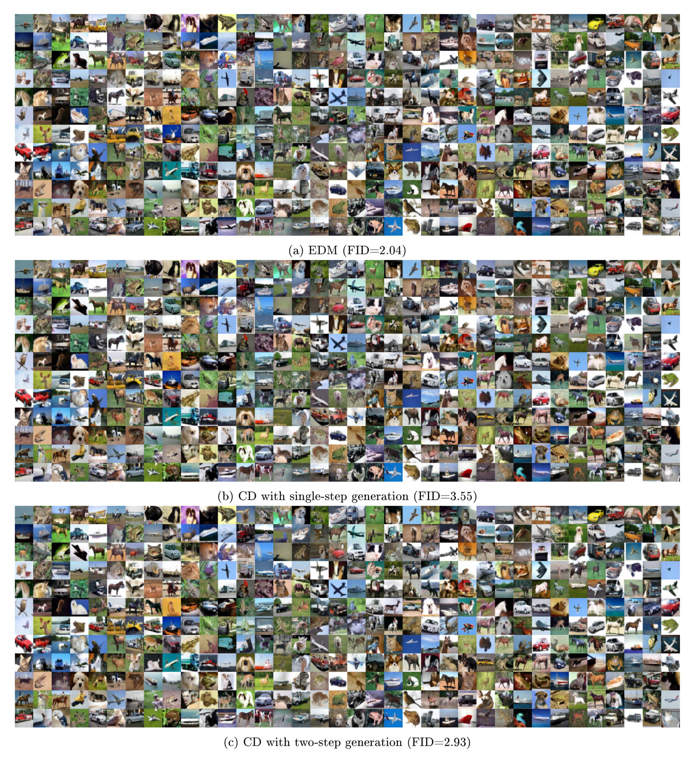
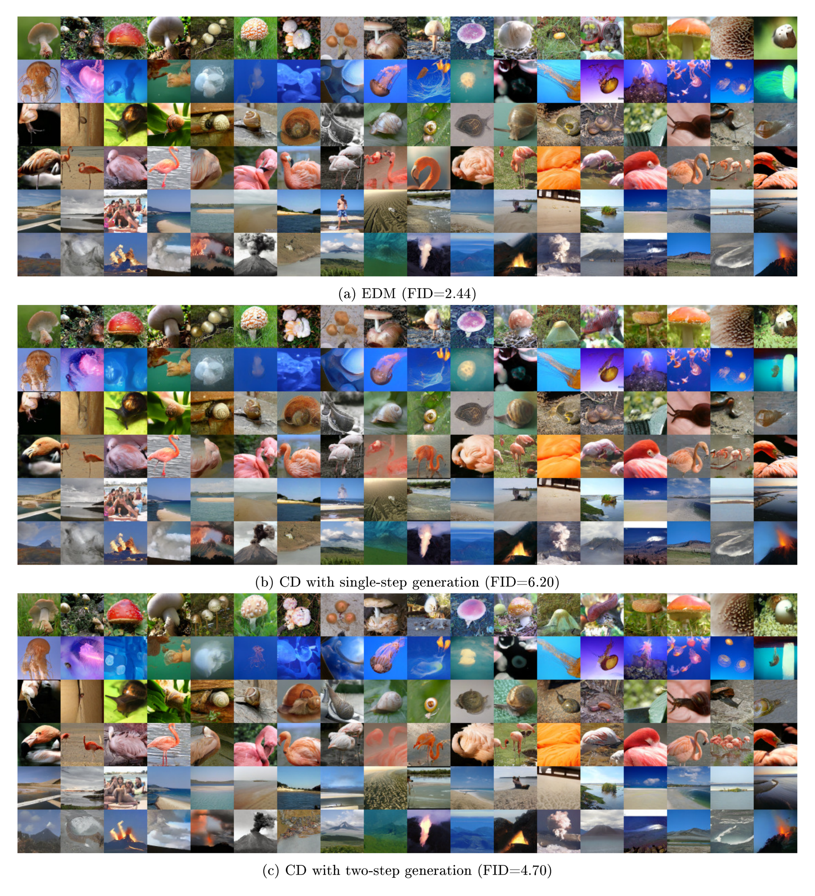
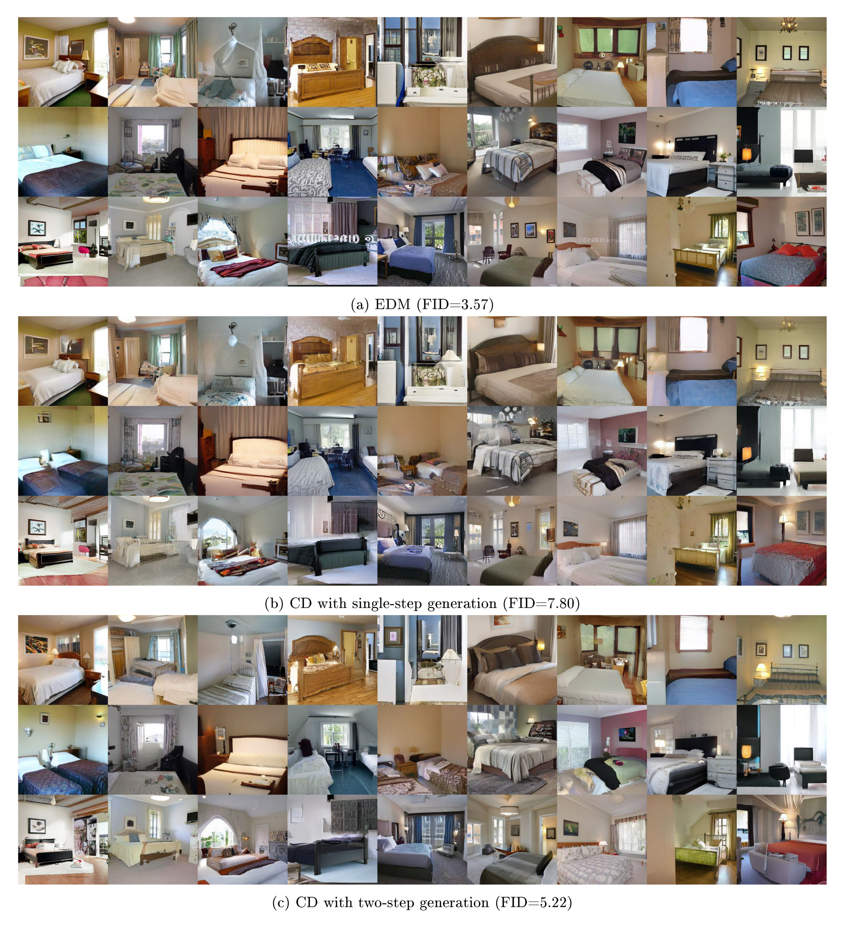
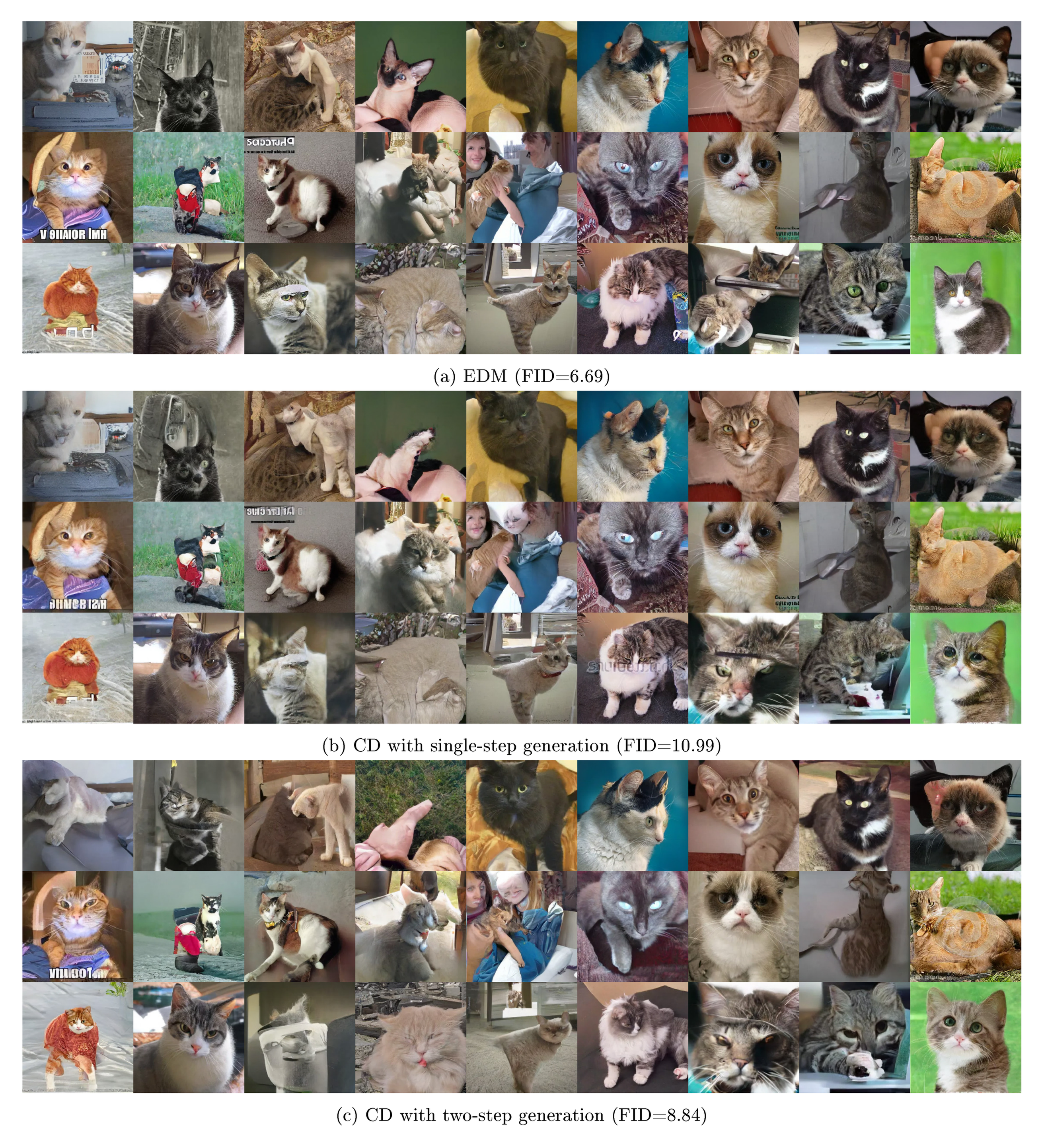
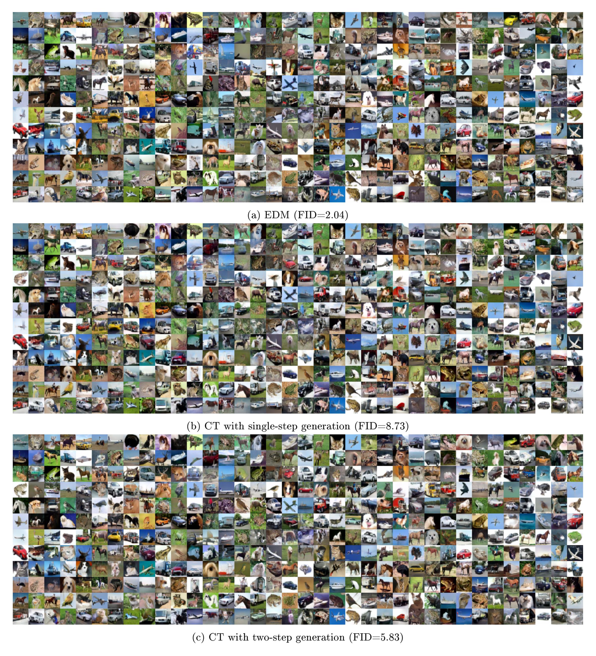
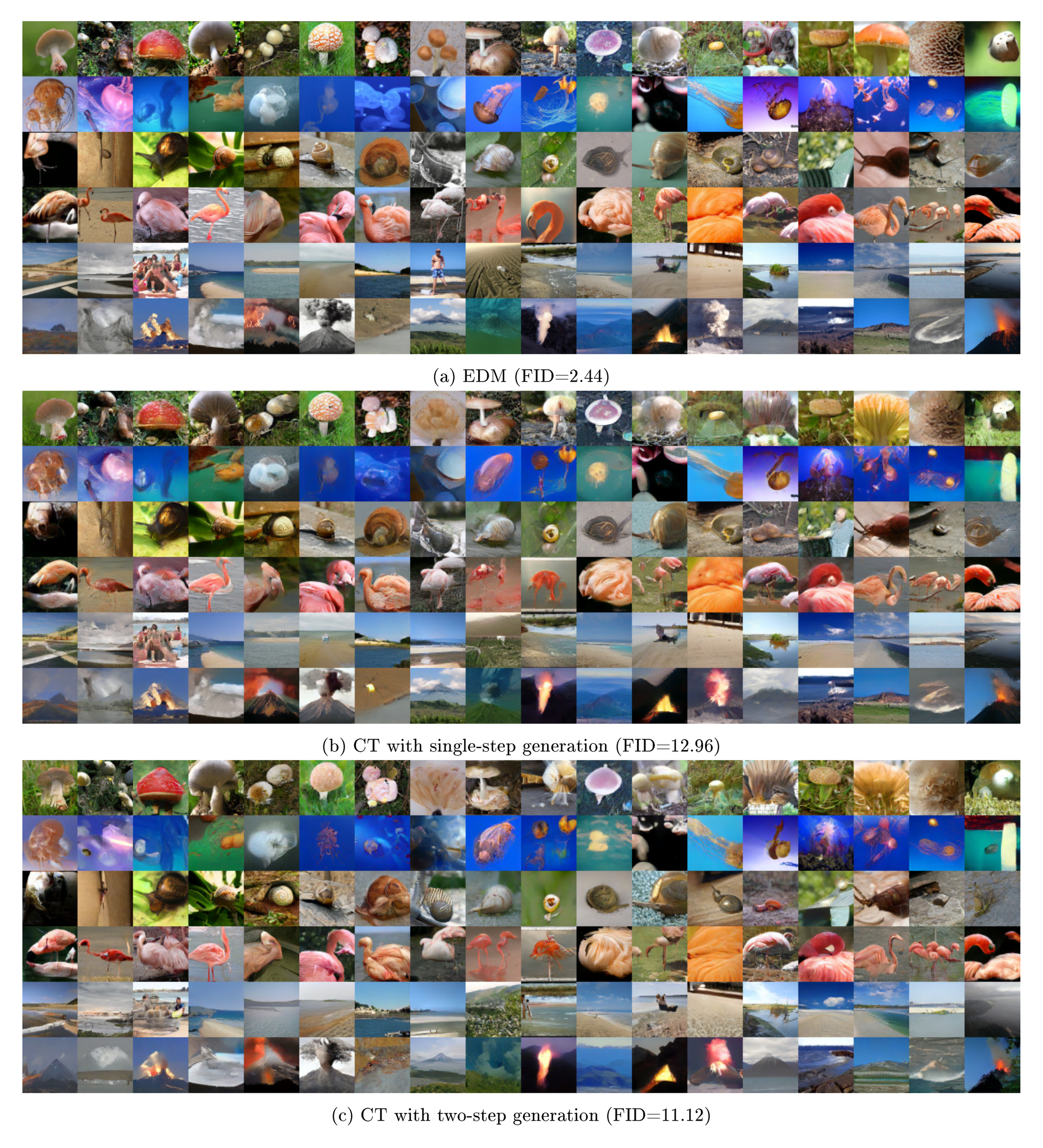
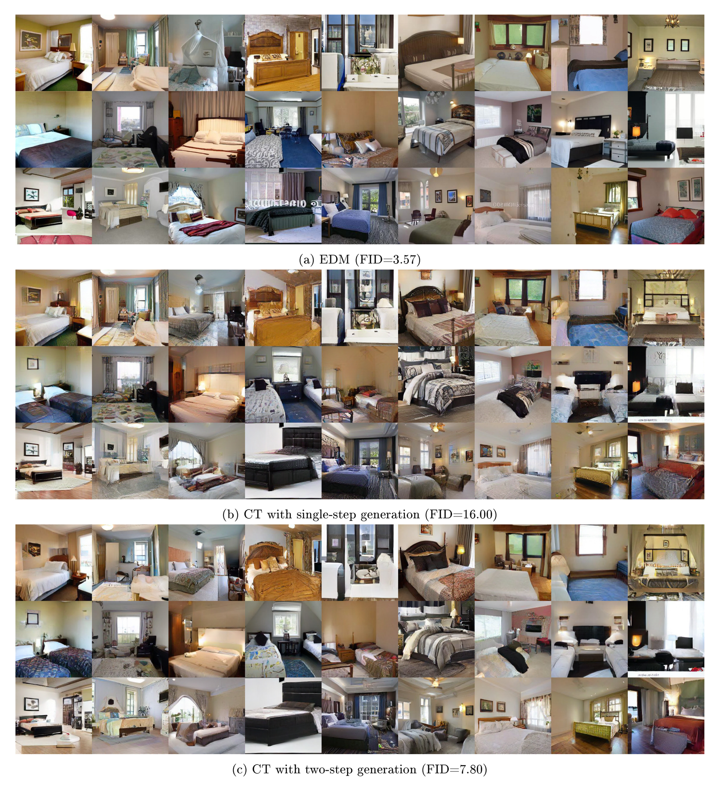
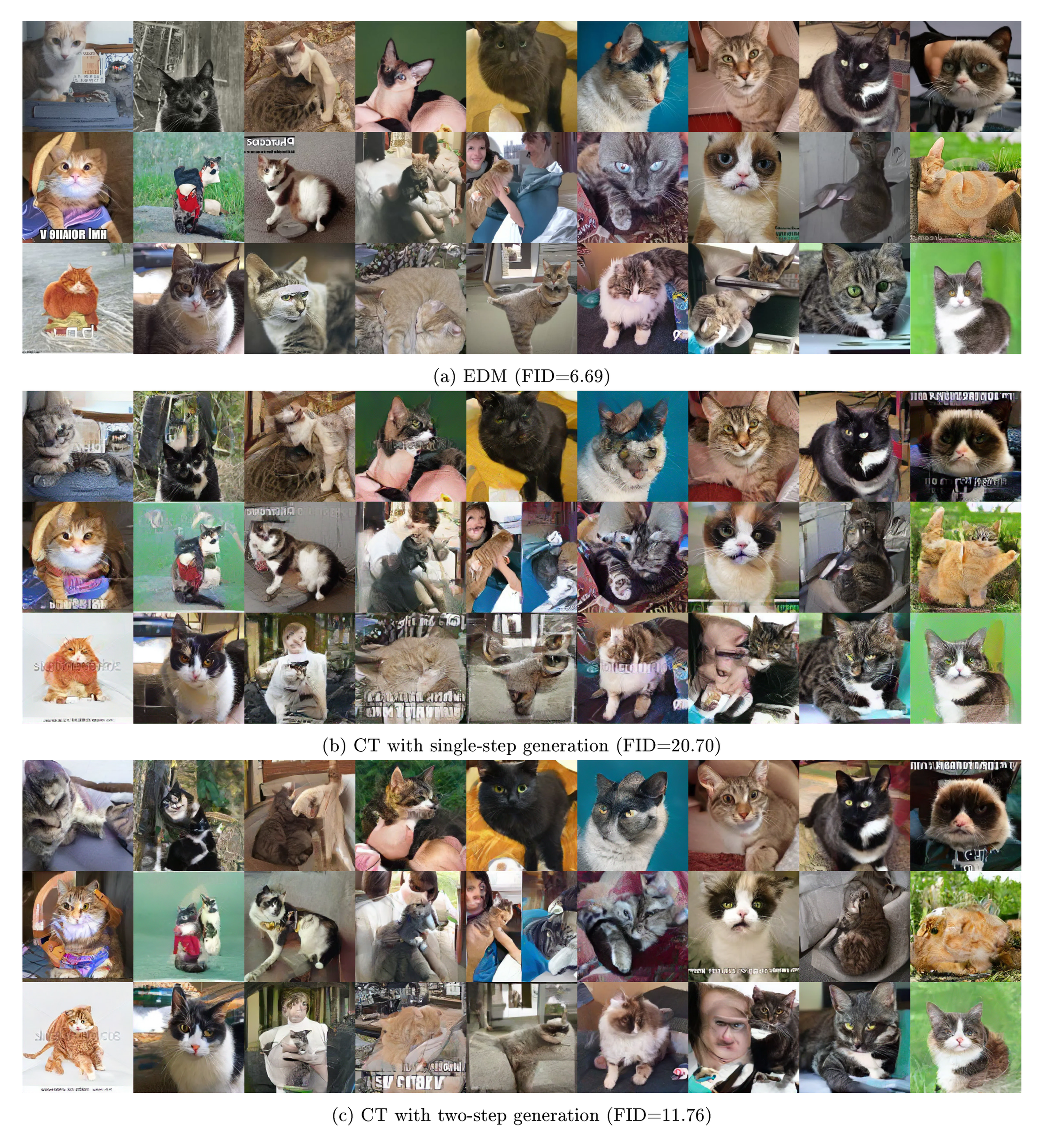
Failed to load: **Figure 5:** Samples generated by EDM (*top*), CT + single-step generation (*middle*), and CT + 2-step generation (*Bottom*). All corresponding images are generated from the same initial noise.
Figure 5: Samples generated by EDM (top), CT + single-step generation (middle), and CT + 2-step generation (Bottom). All corresponding images are generated from the same initial noise.
💭 Click to ask about this figure
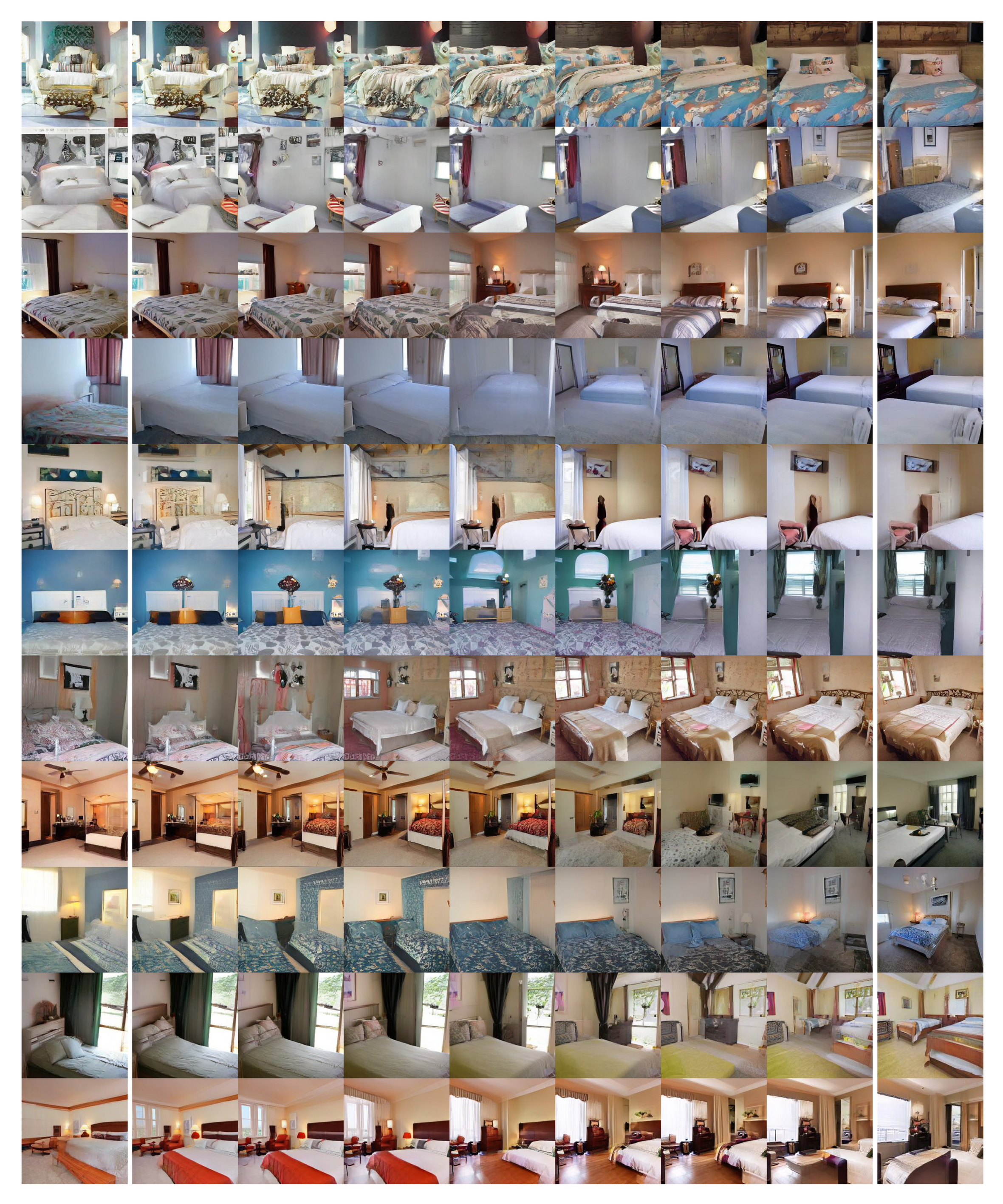
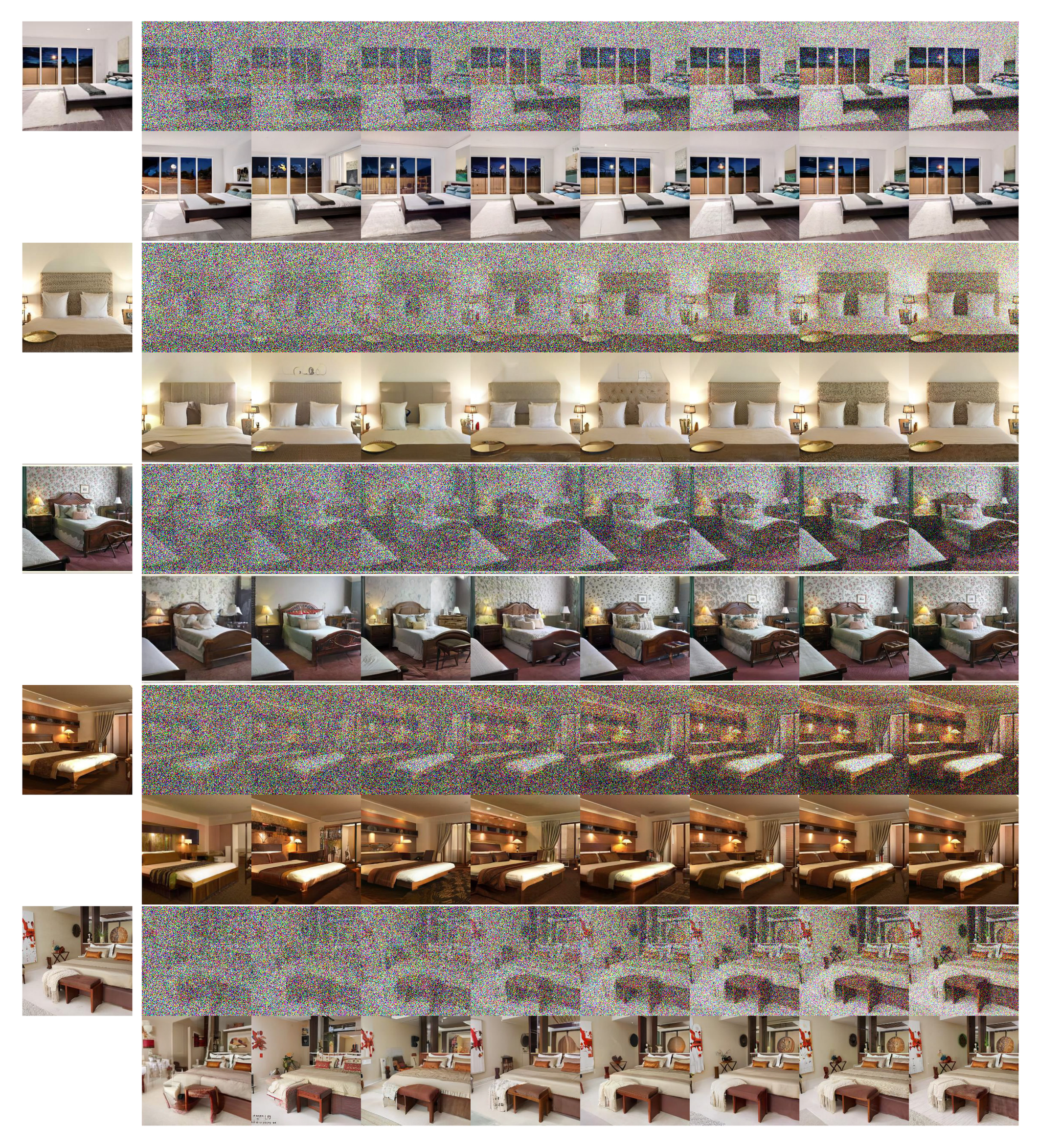
Failed to load: **Figure 6:** Zero-shot image editing with a consistency model trained by consistency distillation on LSUN Bedroom $256\times 256$.
Figure 6: Zero-shot image editing with a consistency model trained by consistency distillation on LSUN Bedroom 256×256.
💭 Click to ask about this figure
Direct Generation In Table 1 and Table 2, we compare the sample quality of consistency training (CT) with other generative models using one-step and two-step generation. We also include PD and CD results for reference. Both tables report PD results obtained from the ℓ2\ell_2ℓ2 metric function, as this is the default setting used in the original paper of [33]. For fair comparison, we ensure PD and CD distill the same EDM models. In Table 1 and Table 2, we observe that CT outperforms existing single-step, non-adversarial generative models, i.e, VAEs and normalizing flows, by a significant margin on CIFAR-10. Moreover, CT achieves comparable quality to one-step samples from PD without relying on distillation. In Figure 5, we provide EDM samples (top), single-step CT samples (middle), and two-step CT samples (bottom). In Appendix E, we show additional samples for both CD and CT in Figure 14, Figure 15, Figure 16, Figure 17, Figure 18, Figure 19, Figure 20, and Figure 21. Importantly, all samples obtained from the same initial noise vector share significant structural similarity, even though CT and EDM models are trained independently from one another. This indicates that CT is less likely to suffer from mode collapse, as EDMs do not.
6.3 Zero-Shot Image Editing
Similar to diffusion models, consistency models allow zero-shot image editing by modifying the multistep sampling process in Algorithm 1. We demonstrate this capability with a consistency model trained on the LSUN bedroom dataset using consistency distillation. In Figure 6a, we show such a consistency model can colorize gray-scale bedroom images at test time, even though it has never been trained on colorization tasks. In Figure 6b, we show the same consistency model can generate high-resolution images from low-resolution inputs. In Figure 6c, we additionally demonstrate that it can generate images based on stroke inputs created by humans, as in SDEdit for diffusion models [21]. Again, this editing capability is zero-shot, as the model has not been trained on stroke inputs. In Appendix D, we additionally demonstrate the zero-shot capability of consistency models on inpainting (Figure 10), interpolation (Figure 11) and denoising (Figure 12), with more examples on colorization (Figure 8), super-resolution (Figure 9) and stroke-guided image generation (Figure 13).
7. Conclusion
Show me a brief summary.
In this section, consistency models emerge as generative models engineered for one-step and few-step image synthesis, tackling slow diffusion-based sampling. Consistency distillation excels over prior techniques on diverse benchmarks with minimal iterations, while these models, trained standalone, yield superior single-step samples versus non-GAN rivals and enable zero-shot editing like inpainting, colorization, super-resolution, denoising, interpolation, and stroke guidance—mirroring diffusion capabilities. Their affinities with deep Q-learning and momentum contrastive learning herald cross-disciplinary innovations.
We have introduced consistency models, a type of generative models that are specifically designed to support one-step and few-step generation. We have empirically demonstrated that our consistency distillation method outshines the existing distillation techniques for diffusion models on multiple image benchmarks and small sampling iterations. Furthermore, as a standalone generative model, consistency models generate better samples than existing single-step generation models except for GANs. Similar to diffusion models, they also allow zero-shot image editing applications such as inpainting, colorization, super-resolution, denoising, interpolation, and stroke-guided image generation.
In addition, consistency models share striking similarities with techniques employed in other fields, including deep Q-learning [48] and momentum-based contrastive learning [50, 51]. This offers exciting prospects for cross-pollination of ideas and methods among these diverse fields.
Acknowledgements
Show me a brief summary.
In this section, recognizing essential collaborators behind the consistency models research stands as a core gesture of academic gratitude. It credits Alex Nichol for rigorous manuscript review and feedback, Chenlin Meng for crucial stroke inputs enabling stroke-guided image generation experiments, and the OpenAI Algorithms team for broader support. This underscores how targeted contributions from individuals and teams propel breakthroughs in one-step generative modeling to superior sample quality and zero-shot editing capabilities.
We thank Alex Nichol for reviewing the manuscript and providing valuable feedback, Chenlin Meng for providing stroke inputs needed in our stroke-guided image generation experiments, and the OpenAI Algorithms team.
Appendix
A. Proofs
A.1 Notations
We use fθ(x,t){\bm{f}}_{{\bm{\theta}}}({\mathbf{x}}, t)fθ(x,t) to denote a consistency model parameterized by θ{\bm{\theta}}θ, and f(x,t;ϕ){\bm{f}}({\mathbf{x}}, t; {\bm{\phi}})f(x,t;ϕ) the consistency function of the empirical PF ODE in Equation 3. Here ϕ{\bm{\phi}}ϕ symbolizes its dependency on the pre-trained score model vs.ϕ(x,t)\emph{vs}._{\bm{\phi}}({\mathbf{x}}, t)vs.ϕ(x,t). For the consistency function of the PF ODE in Equation 2, we denote it as f(x,t){\bm{f}}({\mathbf{x}}, t)f(x,t). Given a multi-variate function h(x,y){\bm{h}}({\mathbf{x}}, {\mathbf{y}})h(x,y), we let ∂1h(x,y)\partial_1 {\bm{h}}({\mathbf{x}}, {\mathbf{y}})∂1h(x,y) denote the Jacobian of h{\bm{h}}h over x{\mathbf{x}}x, and analogously ∂2h(x,y)\partial_2 {\bm{h}}({\mathbf{x}}, {\mathbf{y}})∂2h(x,y) denote the Jacobian of h{\bm{h}}h over y{\mathbf{y}}y. Unless otherwise stated, x{\mathbf{x}}x is supposed to be a random variable sampled from the data distribution pdata(x)p_\text{data}({\mathbf{x}})pdata(x), nnn is sampled uniformly at random from ⟦1,N−1⟧\llbracket 1, N-1 \rrbracket[[1,N−1]], and xtn{\mathbf{x}}_{t_{n}}xtn is sampled from N(x;tn2I)\mathcal{N}({\mathbf{x}}; t_n^2 {\bm{I}})N(x;tn2I). Here ⟦1,N−1⟧\llbracket 1, N-1 \rrbracket[[1,N−1]] represents the set of integers {1,2,⋯ ,N−1}\{1, 2, \cdots, N-1\}{1,2,⋯,N−1}. Furthermore, recall that we define
x^tnϕ:=xtn+1+(tn−tn+1)Φ(xtn+1,tn+1;ϕ),
💭 Click to ask about this equation
where Φ(⋯ ;ϕ)\Phi(\cdots; {\bm{\phi}})Φ(⋯;ϕ) denotes the update function of a one-step ODE solver for the empirical PF ODE defined by the score model vs.ϕ(x,t)\emph{vs}._{\bm{\phi}}({\mathbf{x}}, t)vs.ϕ(x,t). By default, E[⋅]\mathbb{E}[\cdot]E[⋅] denotes the expectation over all relevant random variables in the expression.
A.2 Consistency Distillation
Theorem 2
Let Δt≔maxn∈⟦1,N−1⟧{∣tn+1−tn∣}\Delta t \coloneqq \max_{n \in \llbracket 1, N-1\rrbracket}\{|t_{n+1} - t_{n}|\}Δt:=maxn∈[[1,N−1]]{∣tn+1−tn∣}, and f(⋅,⋅;ϕ){\bm{f}}(\cdot, \cdot; {\bm{\phi}})f(⋅,⋅;ϕ) be the consistency function of the empirical PF ODE in Equation 3. Assume fθ{\bm{f}}_{\bm{\theta}}fθ satisfies the Lipschitz condition: there exists L>0L > 0L>0 such that for all t∈[ϵ,T]t \in [\epsilon, T]t∈[ϵ,T], x{\mathbf{x}}x, and y{\mathbf{y}}y, we have ∥fθ(x,t)−fθ(y,t)∥2≤L∥x−y∥2\left\lVert {\bm{f}}_{\bm{\theta}}({\mathbf{x}}, t) - {\bm{f}}_{\bm{\theta}}({\mathbf{y}}, t)\right\rVert_2 \leq L \left\lVert {\mathbf{x}} - {\mathbf{y}}\right\rVert_2∥fθ(x,t)−fθ(y,t)∥2≤L∥x−y∥2. Assume further that for all n∈⟦1,N−1⟧n \in \llbracket 1, N-1 \rrbracketn∈[[1,N−1]], the ODE solver called at tn+1t_{n+1}tn+1 has local error uniformly bounded by O((tn+1−tn)p+1)O((t_{n+1} - t_n)^{p+1})O((tn+1−tn)p+1) with p≥1p\geq 1p≥1. Then, if LCDN(θ,θ;ϕ)=0\mathcal{L}_\text{CD}^N({\bm{\theta}}, {\bm{\theta}}; {\bm{\phi}}) = 0LCDN(θ,θ;ϕ)=0, we have
n,xsup∥fθ(x,tn)−f(x,tn;ϕ)∥2=O((Δt)p).
💭 Click to ask about this equation
Proof: From LCDN(θ,θ;ϕ)=0\mathcal{L}_\text{CD}^N({\bm{\theta}}, {\bm{\theta}}; {\bm{\phi}}) = 0LCDN(θ,θ;ϕ)=0, we have
According to the definition, we have ptn(xtn)=pdata(x)⊗N(0,tn2I)p_{t_n}({\mathbf{x}}_{t_n}) = p_\text{data}({\mathbf{x}}) \otimes \mathcal{N}(\bm{0}, t_n^2 {\bm{I}})ptn(xtn)=pdata(x)⊗N(0,tn2I) where tn≥ϵ>0t_n \geq \epsilon > 0tn≥ϵ>0. It follows that ptn(xtn)>0p_{t_n}({\mathbf{x}}_{t_n}) > 0ptn(xtn)>0 for every xtn{\mathbf{x}}_{t_n}xtn and 1≤n≤N1 \leq n \leq N1≤n≤N. Therefore, Equation 11 entails
λ(tn)d(fθ(xtn+1,tn+1),fθ(x^tnϕ,tn))≡0.
💭 Click to ask about this equation
Because λ(⋅)>0\lambda(\cdot) > 0λ(⋅)>0 and d(x,y)=0⇔x=yd({\mathbf{x}}, {\mathbf{y}}) = 0 \Leftrightarrow {\mathbf{x}} = {\mathbf{y}}d(x,y)=0⇔x=y, this further implies that
fθ(xtn+1,tn+1)≡fθ(x^tnϕ,tn).
💭 Click to ask about this equation
(12)
Now let en{\bm{e}}_{n}en represent the error vector at tnt_ntn, which is defined as
en:=fθ(xtn,tn)−f(xtn,tn;ϕ).
💭 Click to ask about this equation
We can easily derive the following recursion relation
where (i) is due to 12 and f(xtn+1,tn+1;ϕ)=f(xtn,tn;ϕ){\bm{f}}({\mathbf{x}}_{t_{n+1}}, t_{n+1}; {\bm{\phi}}) = {\bm{f}}({\mathbf{x}}_{t_{n}}, t_{n}; {\bm{\phi}})f(xtn+1,tn+1;ϕ)=f(xtn,tn;ϕ). Because fθ(⋅,tn){\bm{f}}_{\bm{\theta}}(\cdot, t_n)fθ(⋅,tn) has Lipschitz constant LLL, we have
where (i) holds because the ODE solver has local error bounded by O((tn+1−tn)p+1)O((t_{n+1}-t_n)^{p+1})O((tn+1−tn)p+1). In addition, we observe that e1=0{\bm{e}}_1 = \bm{0}e1=0, because
Here (i) is true because the consistency model is parameterized such that f(xt1,t1;ϕ)=xt1{\bm{f}}({\mathbf{x}}_{t_1}, t_1; {\bm{\phi}}) = {\mathbf{x}}_{t_1}f(xt1,t1;ϕ)=xt1 and (ii) is entailed by the definition of f(⋅,⋅;ϕ){\bm{f}}(\cdot, \cdot; {\bm{\phi}})f(⋅,⋅;ϕ). This allows us to perform induction on the recursion formula Equation 13 to obtain
The following lemma provides an unbiased estimator for the score function, which is crucial to our proof for Theorem 3.
Lemma 4
Let x∼pdata(x){\mathbf{x}} \sim p_\text{data}({\mathbf{x}})x∼pdata(x), xt∼N(x;t2I){\mathbf{x}}_t \sim \mathcal{N}({\mathbf{x}}; t^2 {\bm{I}})xt∼N(x;t2I), and pt(xt)=pdata(x)⊗N(0,t2I)p_t({\mathbf{x}}_t) = p_\text{data}({\mathbf{x}}) \otimes \mathcal{N}(\bm{0}, t^2 {\bm{I}})pt(xt)=pdata(x)⊗N(0,t2I). We have ∇logpt(x)=−E[xt−xt2∣xt]\nabla \log p_t({\mathbf{x}}) = -\mathbb{E}[\frac{{\mathbf{x}}_t - {\mathbf{x}}}{t^2} \mid {\mathbf{x}}_t]∇logpt(x)=−E[t2xt−x∣xt].
Proof: According to the definition of pt(xt)p_t({\mathbf{x}}_t)pt(xt), we have ∇logpt(xt)=∇xtlog∫pdata(x)p(xt∣x) dx\nabla \log p_t({\mathbf{x}}_t) = \nabla_{{\mathbf{x}}_t} \log \int p_\text{data}({\mathbf{x}}) p({\mathbf{x}}_t \mid {\mathbf{x}}) \mathop{}\!\mathrm{d} {\mathbf{x}}∇logpt(xt)=∇xtlog∫pdata(x)p(xt∣x)dx, where p(xt∣x)=N(xt;x,t2I)p({\mathbf{x}}_t \mid {\mathbf{x}}) = \mathcal{N}({\mathbf{x}}_t; {\mathbf{x}}, t^2 {\bm{I}})p(xt∣x)=N(xt;x,t2I). This expression can be further simplified to yield
Theorem 3
Let Δt≔maxn∈⟦1,N−1⟧{∣tn+1−tn∣}\Delta t \coloneqq \max_{n \in \llbracket 1, N-1\rrbracket}\{|t_{n+1} - t_{n}|\}Δt:=maxn∈[[1,N−1]]{∣tn+1−tn∣}. Assume ddd and fθ−{\bm{f}}_{{\bm{\theta}}^{-}}fθ− are both twice continuously differentiable with bounded second derivatives, the weighting function λ(⋅)\lambda(\cdot)λ(⋅) is bounded, and E[∥∇logptn(xtn)∥22]<∞\mathbb{E}[\left\lVert\nabla \log p_{t_n}({\mathbf{x}}_{t_{n}})\right\rVert_2^2] < \inftyE[∥∇logptn(xtn)∥22]<∞. Assume further that we use the Euler ODE solver, and the pre-trained score model matches the ground truth, i.e, ∀t∈[ϵ,T]:vs.ϕ(x,t)≡∇logpt(x)\forall t\in[\epsilon, T]: \emph{vs}._{{\bm{\phi}}}({\mathbf{x}}, t) \equiv \nabla \log p_t({\mathbf{x}})∀t∈[ϵ,T]:vs.ϕ(x,t)≡∇logpt(x). Then,
LCDN(θ,θ−;ϕ)=LCTN(θ,θ−)+o(Δt),
💭 Click to ask about this equation
where the expectation is taken with respect to x∼pdata{\mathbf{x}} \sim p_\text{data}x∼pdata, n∼U⟦1,N−1⟧n \sim \mathcal{U}\llbracket 1, N-1 \rrbracketn∼U[[1,N−1]], and xtn+1∼N(x;tn+12I){\mathbf{x}}_{t_{n+1}} \sim \mathcal{N}({\mathbf{x}}; t_{n+1}^2 {\bm{I}})xtn+1∼N(x;tn+12I). The consistency training objective, denoted by LCTN(θ,θ−)\mathcal{L}_\text{CT}^N({\bm{\theta}}, {\bm{\theta}}^{-})LCTN(θ,θ−), is defined as
where (i) is due to the law of total expectation, and z≔xtn+1−xtn+1∼N(0,I){\mathbf{z}} \coloneqq \frac{{\mathbf{x}}_{t_{n+1}} - {\mathbf{x}}}{t_{n+1}} \sim \mathcal{N}(\bm{0}, {\bm{I}})z:=tn+1xtn+1−x∼N(0,I). This implies LCDN(θ,θ−;ϕ)=LCTN(θ,θ−)+o(Δt)\mathcal{L}_\text{CD}^N({\bm{\theta}}, {\bm{\theta}}^{-}; {\bm{\phi}}) = \mathcal{L}_\text{CT}^N({\bm{\theta}}, {\bm{\theta}}^{-}) + o(\Delta t)LCDN(θ,θ−;ϕ)=LCTN(θ,θ−)+o(Δt) and thus completes the proof for Equation 9. Moreover, we have LCTN(θ,θ−)≥O(Δt)\mathcal{L}_\text{CT}^N({\bm{\theta}}, {\bm{\theta}}^{-}) \geq O(\Delta t)LCTN(θ,θ−)≥O(Δt) whenever infNLCDN(θ,θ−;ϕ)>0\inf_N \mathcal{L}_\text{CD}^N({\bm{\theta}}, {\bm{\theta}}^{-}; {\bm{\phi}}) > 0infNLCDN(θ,θ−;ϕ)>0. Otherwise, LCTN(θ,θ−)<O(Δt)\mathcal{L}_\text{CT}^N({\bm{\theta}}, {\bm{\theta}}^{-}) < O(\Delta t)LCTN(θ,θ−)<O(Δt) and thus limΔt→0LCDN(θ,θ−;ϕ)=0\lim_{\Delta t \to 0} \mathcal{L}_\text{CD}^N({\bm{\theta}}, {\bm{\theta}}^{-}; {\bm{\phi}}) = 0limΔt→0LCDN(θ,θ−;ϕ)=0, which is a clear contradiction to infNLCDN(θ,θ−;ϕ)>0\inf_N \mathcal{L}_\text{CD}^N({\bm{\theta}}, {\bm{\theta}}^{-}; {\bm{\phi}}) > 0infNLCDN(θ,θ−;ϕ)>0.
Remark.
When the condition LCTN(θ,θ−)≥O(Δt)\mathcal{L}_\text{CT}^N({\bm{\theta}}, {\bm{\theta}}^{-}) \geq O(\Delta t)LCTN(θ,θ−)≥O(Δt) is not satisfied, such as in the case where θ−=stopgrad(θ){\bm{\theta}}^{-} = \operatorname{stopgrad}({\bm{\theta}})θ−=stopgrad(θ), the validity of LCTN(θ,θ−)\mathcal{L}_\text{CT}^N({\bm{\theta}}, {\bm{\theta}}^{-})LCTN(θ,θ−) as a training objective for consistency models can still be justified by referencing the result provided in Theorem 10.
B. Continuous-Time Extensions
The consistency distillation and consistency training objectives can be generalized to hold for infinite time steps (N→∞N\to\inftyN→∞) under suitable conditions.
B.1 Consistency Distillation in Continuous Time
Depending on whether θ−=θ{\bm{\theta}}^- = {\bm{\theta}}θ−=θ or θ−=stopgrad(θ){\bm{\theta}}^- = \operatorname{stopgrad}({\bm{\theta}})θ−=stopgrad(θ) (same as setting μ=0\mu=0μ=0), there are two possible continuous-time extensions for the consistency distillation objective LCDN(θ,θ−;ϕ)\mathcal{L}_\text{CD}^N({\bm{\theta}}, {\bm{\theta}}^{-}; {\bm{\phi}})LCDN(θ,θ−;ϕ). Given a twice continuously differentiable metric function d(x,y)d({\mathbf{x}}, {\mathbf{y}})d(x,y), we define G(x){\bm{G}}({\mathbf{x}})G(x) as a matrix, whose (i,j)(i, j)(i,j)-th entry is given by
[G(x)]ij:=∂yi∂yj∂2d(x,y)y=x.
💭 Click to ask about this equation
Similarly, we define H(x){\bm{H}}({\mathbf{x}})H(x) as
[H(x)]ij:=∂yi∂yj∂2d(y,x)y=x.
💭 Click to ask about this equation
The matrices G{\bm{G}}G and H{\bm{H}}H play a crucial role in forming continuous-time objectives for consistency distillation. Additionally, we denote the Jacobian of fθ(x,t){\bm{f}}_{\bm{\theta}}({\mathbf{x}}, t)fθ(x,t) with respect to x{\mathbf{x}}x as ∂fθ(x,t)∂x\frac{\partial {\bm{f}}_{\bm{\theta}}({\mathbf{x}}, t)}{\partial {\mathbf{x}}}∂x∂fθ(x,t).
When θ−=θ{\bm{\theta}}^{-}= {\bm{\theta}}θ−=θ (with no stopgrad operator), we have the following theoretical result.
Theorem 5
Let tn=τ(n−1N−1)t_n = \tau(\frac{n-1}{N-1})tn=τ(N−1n−1), where n∈⟦1,N⟧n \in \llbracket 1, N \rrbracketn∈[[1,N]], and τ(⋅)\tau(\cdot)τ(⋅) is a strictly monotonic function with τ(0)=ϵ\tau(0) = \epsilonτ(0)=ϵ and τ(1)=T\tau(1) = Tτ(1)=T. Assume τ\tauτ is continuously differentiable in [0,1][0, 1][0,1], ddd is three times continuously differentiable with bounded third derivatives, and fθ{\bm{f}}_{{\bm{\theta}}}fθ is twice continuously differentiable with bounded first and second derivatives. Assume further that the weighting function λ(⋅)\lambda(\cdot)λ(⋅) is bounded, and supx,t∈[ϵ,T]∥vs.ϕ(x,t)∥2<∞\sup_{{\mathbf{x}}, t\in[\epsilon, T]}\left\lVert \emph{vs}._{\bm{\phi}}({\mathbf{x}}, t)\right\rVert_2 < \inftysupx,t∈[ϵ,T]∥vs.ϕ(x,t)∥2<∞. Then with the Euler solver in consistency distillation, we have
N→∞lim(N−1)2LCDN(θ,θ;ϕ)=LCD∞(θ,θ;ϕ),
💭 Click to ask about this equation
(15)
where LCD∞(θ,θ;ϕ)\mathcal{L}_\text{CD}^{\infty} ({\bm{\theta}}, {\bm{\theta}}; {\bm{\phi}})LCD∞(θ,θ;ϕ) is defined as
Here the expectation above is taken over x∼pdata{\mathbf{x}} \sim p_\text{data}x∼pdata, u∼U[0,1]u \sim \mathcal{U}[0, 1]u∼U[0,1], t=τ(u)t = \tau(u)t=τ(u), and xt∼N(x,t2I){\mathbf{x}}_t \sim \mathcal{N}({\mathbf{x}}, t^2 {\bm{I}})xt∼N(x,t2I).
Proof: Let Δu=1N−1\Delta u = \frac{1}{N-1}Δu=N−11 and un=n−1N−1u_n = \frac{n-1}{N-1}un=N−1n−1. First, we can derive the following equation with Taylor expansion:
Note that τ′(un)=1τ−1(tn+1)\tau'(u_{n}) = \frac{1}{\tau^{-1}(t_{n+1})}τ′(un)=τ−1(tn+1)1. Then, we apply Taylor expansion to the consistency distillation loss, which gives
where we obtain (i) by expanding d(fθ(xtn+1,tn+1),⋅)d({\bm{f}}_{\bm{\theta}}({\mathbf{x}}_{t_{n+1}}, t_{n+1}), \cdot)d(fθ(xtn+1,tn+1),⋅) to second order and observing d(x,x)≡0d({\mathbf{x}}, {\mathbf{x}}) \equiv 0d(x,x)≡0 and ∇yd(x,y)∣y=x≡0\nabla_{\mathbf{y}} d({\mathbf{x}}, {\mathbf{y}})|_{{\mathbf{y}}= {\mathbf{x}}} \equiv \bm{0}∇yd(x,y)∣y=x≡0. We obtain (ii) using Equation 16. By taking the limit for both sides of Equation 17 as Δu→0\Delta u \to 0Δu→0 or equivalently N→∞N \to \inftyN→∞, we arrive at Equation 15, which completes the proof.
Remark.
Although Theorem 5 assumes the Euler ODE solver for technical simplicity, we believe an analogous result can be derived for more general solvers, since all ODE solvers should perform similarly as N→∞N \to \inftyN→∞. We leave a more general version of Theorem 5 as future work.
Remark.
Theorem 5 implies that consistency models can be trained by minimizing LCD∞(θ,θ;ϕ)\mathcal{L}_\text{CD}^\infty ({\bm{\theta}}, {\bm{\theta}}; {\bm{\phi}})LCD∞(θ,θ;ϕ). In particular, when d(x,y)=∥x−y∥22d({\mathbf{x}}, {\mathbf{y}}) = \left\lVert {\mathbf{x}} - {\mathbf{y}}\right\rVert_2^2d(x,y)=∥x−y∥22, we have
However, this continuous-time objective requires computing Jacobian-vector products as a subroutine to evaluate the loss function, which can be slow and laborious to implement in deep learning frameworks that do not support forward-mode automatic differentiation.
Remark 6
If fθ(x,t){\bm{f}}_{\bm{\theta}}({\mathbf{x}}, t)fθ(x,t) matches the ground truth consistency function for the empirical PF ODE of vs.ϕ(x,t)\emph{vs}._{\bm{\phi}}({\mathbf{x}}, t)vs.ϕ(x,t), then
∂t∂fθ(x,t)−t∂x∂fθ(x,t)vs.ϕ(x,t)≡0
💭 Click to ask about this equation
and therefore LCD∞(θ,θ;ϕ)=0\mathcal{L}_\text{CD}^\infty({\bm{\theta}}, {\bm{\theta}}; {\bm{\phi}}) = 0LCD∞(θ,θ;ϕ)=0. This can be proved by noting that fθ(xt,t)≡xϵ{\bm{f}}_{\bm{\theta}}({\mathbf{x}}_t, t) \equiv {\mathbf{x}}_\epsilonfθ(xt,t)≡xϵ for all t∈[ϵ,T]t \in [\epsilon, T]t∈[ϵ,T], and then taking the time-derivative of this identity:
The above observation provides another motivation for LCD∞(θ,θ;ϕ)\mathcal{L}_\text{CD}^\infty({\bm{\theta}}, {\bm{\theta}}; {\bm{\phi}})LCD∞(θ,θ;ϕ), as it is minimized if and only if the consistency model matches the ground truth consistency function.
For some metric functions, such as the ℓ1\ell_1ℓ1 norm, the Hessian G(x){\bm{G}}({\mathbf{x}})G(x) is zero so Theorem 5 is vacuous. Below we show that a non-vacuous statement holds for the ℓ1\ell_1ℓ1 norm with just a small modification of the proof for Theorem 5.
Theorem 7
Let tn=τ(n−1N−1)t_n = \tau(\frac{n-1}{N-1})tn=τ(N−1n−1), where n∈⟦1,N⟧n \in \llbracket 1, N \rrbracketn∈[[1,N]], and τ(⋅)\tau(\cdot)τ(⋅) is a strictly monotonic function with τ(0)=ϵ\tau(0) = \epsilonτ(0)=ϵ and τ(1)=T\tau(1) = Tτ(1)=T. Assume τ\tauτ is continuously differentiable in [0,1][0, 1][0,1], and fθ{\bm{f}}_{{\bm{\theta}}}fθ is twice continuously differentiable with bounded first and second derivatives. Assume further that the weighting function λ(⋅)\lambda(\cdot)λ(⋅) is bounded, and supx,t∈[ϵ,T]∥vs.ϕ(x,t)∥2<∞\sup_{{\mathbf{x}}, t\in[\epsilon, T]}\left\lVert \emph{vs}._{\bm{\phi}}({\mathbf{x}}, t)\right\rVert_2 < \inftysupx,t∈[ϵ,T]∥vs.ϕ(x,t)∥2<∞. Suppose we use the Euler ODE solver, and set d(x,y)=∥x−y∥1d({\mathbf{x}}, {\mathbf{y}}) = \left\lVert {\mathbf{x}} - {\mathbf{y}}\right\rVert_1d(x,y)=∥x−y∥1 in consistency distillation. Then we have
where the expectation above is taken over x∼pdata{\mathbf{x}} \sim p_\text{data}x∼pdata, u∼U[0,1]u \sim \mathcal{U}[0, 1]u∼U[0,1], t=τ(u)t = \tau(u)t=τ(u), and xt∼N(x,t2I){\mathbf{x}}_t \sim \mathcal{N}({\mathbf{x}}, t^2 {\bm{I}})xt∼N(x,t2I).
Proof: Let Δu=1N−1\Delta u = \frac{1}{N-1}Δu=N−11 and un=n−1N−1u_n = \frac{n-1}{N-1}un=N−1n−1. We have
where (i) is obtained by plugging Equation 16 into the previous equation. Taking the limit for both sides of Equation 19 as Δu→0\Delta u \to 0Δu→0 or equivalently N→∞N\to \inftyN→∞ leads to 18, which completes the proof.
Remark.
According to Theorem 7, consistency models can be trained by minimizing LCD, ℓ1∞(θ,θ;ϕ)\mathcal{L}_\text{CD, $ \ell_1 $}^\infty({\bm{\theta}}, {\bm{\theta}}; {\bm{\phi}})LCD, ℓ1∞(θ,θ;ϕ). Moreover, the same reasoning in Remark 6 can be applied to show that LCD, ℓ1∞(θ,θ;ϕ)=0\mathcal{L}_\text{CD, $ \ell_1 $}^\infty({\bm{\theta}}, {\bm{\theta}}; {\bm{\phi}}) = 0LCD, ℓ1∞(θ,θ;ϕ)=0 if and only if fθ(xt,t)=xϵ{\bm{f}}_{\bm{\theta}}({\mathbf{x}}_t, t) = {\mathbf{x}}_\epsilonfθ(xt,t)=xϵ for all xt∈Rd{\mathbf{x}}_t \in \mathbb{R}^dxt∈Rd and t∈[ϵ,T]t \in [\epsilon, T]t∈[ϵ,T].
In the second case where θ−=stopgrad(θ){\bm{\theta}}^- = \operatorname{stopgrad}({\bm{\theta}})θ−=stopgrad(θ), we can derive a so-called "pseudo-objective" whose gradient matches the gradient of LCDN(θ,θ−;ϕ)\mathcal{L}_\text{CD}^N({\bm{\theta}}, {\bm{\theta}}^{-}; {\bm{\phi}})LCDN(θ,θ−;ϕ) in the limit of N→∞N\to\inftyN→∞. Minimizing this pseudo-objective with gradient descent gives another way to train consistency models via distillation. This pseudo-objective is provided by the theorem below.
Theorem 8
Let tn=τ(n−1N−1)t_n = \tau(\frac{n-1}{N-1})tn=τ(N−1n−1), where n∈⟦1,N⟧n \in \llbracket 1, N \rrbracketn∈[[1,N]], and τ(⋅)\tau(\cdot)τ(⋅) is a strictly monotonic function with τ(0)=ϵ\tau(0) = \epsilonτ(0)=ϵ and τ(1)=T\tau(1) = Tτ(1)=T. Assume τ\tauτ is continuously differentiable in [0,1][0, 1][0,1], ddd is three times continuously differentiable with bounded third derivatives, and fθ{\bm{f}}_{{\bm{\theta}}}fθ is twice continuously differentiable with bounded first and second derivatives. Assume further that the weighting function λ(⋅)\lambda(\cdot)λ(⋅) is bounded, supx,t∈[ϵ,T]∥vs.ϕ(x,t)∥2<∞\sup_{{\mathbf{x}}, t\in[\epsilon, T]}\left\lVert \emph{vs}._{\bm{\phi}}({\mathbf{x}}, t)\right\rVert_2 < \inftysupx,t∈[ϵ,T]∥vs.ϕ(x,t)∥2<∞, and supx,t∈[ϵ,T]∥∇θfθ(x,t)∥2<∞\sup_{{\mathbf{x}}, t\in[\epsilon, T]}\left\lVert\nabla_{\bm{\theta}} {\bm{f}}_{\bm{\theta}}({\mathbf{x}}, t)\right\rVert_2 < \inftysupx,t∈[ϵ,T]∥∇θfθ(x,t)∥2<∞. Suppose we use the Euler ODE solver, and θ−=stopgrad(θ){\bm{\theta}}^{-} = \operatorname{stopgrad}({\bm{\theta}})θ−=stopgrad(θ) in consistency distillation. Then,
Here the expectation above is taken over x∼pdata{\mathbf{x}} \sim p_\text{data}x∼pdata, u∼U[0,1]u \sim \mathcal{U}[0, 1]u∼U[0,1], t=τ(u)t = \tau(u)t=τ(u), and xt∼N(x,t2I){\mathbf{x}}_t \sim \mathcal{N}({\mathbf{x}}, t^2 {\bm{I}})xt∼N(x,t2I).
Proof: We denote Δu=1N−1\Delta u = \frac{1}{N-1}Δu=N−11 and un=n−1N−1u_n = \frac{n-1}{N-1}un=N−1n−1. First, we leverage Taylor series expansion to obtain
where (i) is derived by expanding d(⋅,fθ−(x^tnϕ,tn))d(\cdot, {\bm{f}}_{{\bm{\theta}}^{-}}(\hat{{\mathbf{x}}}_{t_n}^{\bm{\phi}}, t_n))d(⋅,fθ−(x^tnϕ,tn)) to second order and leveraging d(x,x)≡0d({\mathbf{x}}, {\mathbf{x}}) \equiv 0d(x,x)≡0 and ∇yd(y,x)∣y=x≡0\nabla_{\mathbf{y}} d({\mathbf{y}}, {\mathbf{x}})|_{{\mathbf{y}}= {\mathbf{x}}} \equiv \bm{0}∇yd(y,x)∣y=x≡0. Next, we compute the gradient of Equation 21 with respect to θ{\bm{\theta}}θ and simplify the result to obtain
Here (i) results from the chain rule, and (ii) follows from Equation 16 and fθ(x,t)≡fθ−(x,t){\bm{f}}_{\bm{\theta}}({\mathbf{x}}, t) \equiv {\bm{f}}_{{\bm{\theta}}^{-}}({\mathbf{x}}, t)fθ(x,t)≡fθ−(x,t), since θ−=stopgrad(θ){\bm{\theta}}^{-} = \operatorname{stopgrad}({\bm{\theta}})θ−=stopgrad(θ). Taking the limit for both sides of Equation 22 as Δu→0\Delta u \to 0Δu→0 (or N→∞N\to\inftyN→∞) yields Equation 20, which completes the proof.
Remark.
When d(x,y)=∥x−y∥22d({\mathbf{x}}, {\mathbf{y}}) = \left\lVert {\mathbf{x}} - {\mathbf{y}}\right\rVert_2^2d(x,y)=∥x−y∥22, the pseudo-objective LCD∞(θ,θ−;ϕ)\mathcal{L}_\text{CD}^\infty ({\bm{\theta}}, {\bm{\theta}}^{-}; {\bm{\phi}})LCD∞(θ,θ−;ϕ) can be simplified to
The objective LCD∞(θ,θ−;ϕ)\mathcal{L}_\text{CD}^\infty({\bm{\theta}}, {\bm{\theta}}^{-}; {\bm{\phi}})LCD∞(θ,θ−;ϕ) defined in Theorem 8 is only meaningful in terms of its gradient—one cannot measure the progress of training by tracking the value of LCD∞(θ,θ−;ϕ)\mathcal{L}_\text{CD}^\infty({\bm{\theta}}, {\bm{\theta}}^{-}; {\bm{\phi}})LCD∞(θ,θ−;ϕ), but can still apply gradient descent to this objective to distill consistency models from pre-trained diffusion models. Because this objective is not a typical loss function, we refer to it as the "pseudo-objective" for consistency distillation.
Remark 9
Following the same reasoning in Remark 6, we can easily derive that LCD∞(θ,θ−;ϕ)=0\mathcal{L}_\text{CD}^\infty({\bm{\theta}}, {\bm{\theta}}^{-}; {\bm{\phi}}) = 0LCD∞(θ,θ−;ϕ)=0 and ∇θLCD∞(θ,θ−;ϕ)=0\nabla_{\bm{\theta}} \mathcal{L}_\text{CD}^\infty({\bm{\theta}}, {\bm{\theta}}^{-}; {\bm{\phi}}) = \bm{0}∇θLCD∞(θ,θ−;ϕ)=0 if fθ(x,t){\bm{f}}_{\bm{\theta}}({\mathbf{x}}, t)fθ(x,t) matches the ground truth consistency function for the empirical PF ODE that involves vs.ϕ(x,t)\emph{vs}._{\bm{\phi}}({\mathbf{x}}, t)vs.ϕ(x,t). However, the converse does not hold true in general. This distinguishes LCD∞(θ,θ−;ϕ)\mathcal{L}_\text{CD}^\infty({\bm{\theta}}, {\bm{\theta}}^{-}; {\bm{\phi}})LCD∞(θ,θ−;ϕ) from LCD∞(θ,θ;ϕ)\mathcal{L}_\text{CD}^\infty({\bm{\theta}}, {\bm{\theta}}; {\bm{\phi}})LCD∞(θ,θ;ϕ), the latter of which is a true loss function.
B.2 Consistency Training in Continuous Time
A remarkable observation is that the pseudo-objective in Theorem 8 can be estimated without any pre-trained diffusion models, which enables direct consistency training of consistency models. More precisely, we have the following result.
Theorem 10
Let tn=τ(n−1N−1)t_n = \tau(\frac{n-1}{N-1})tn=τ(N−1n−1), where n∈⟦1,N⟧n \in \llbracket 1, N \rrbracketn∈[[1,N]], and τ(⋅)\tau(\cdot)τ(⋅) is a strictly monotonic function with τ(0)=ϵ\tau(0) = \epsilonτ(0)=ϵ and τ(1)=T\tau(1) = Tτ(1)=T. Assume τ\tauτ is continuously differentiable in [0,1][0, 1][0,1], ddd is three times continuously differentiable with bounded third derivatives, and fθ{\bm{f}}_{{\bm{\theta}}}fθ is twice continuously differentiable with bounded first and second derivatives. Assume further that the weighting function λ(⋅)\lambda(\cdot)λ(⋅) is bounded, E[∥∇logptn(xtn)∥22]<∞\mathbb{E}[\left\lVert\nabla \log p_{t_n}({\mathbf{x}}_{t_{n}})\right\rVert_2^2] < \inftyE[∥∇logptn(xtn)∥22]<∞, supx,t∈[ϵ,T]∥∇θfθ(x,t)∥2<∞\sup_{{\mathbf{x}}, t\in[\epsilon, T]}\left\lVert\nabla_{\bm{\theta}} {\bm{f}}_{\bm{\theta}}({\mathbf{x}}, t)\right\rVert_2 < \inftysupx,t∈[ϵ,T]∥∇θfθ(x,t)∥2<∞, and ϕ{\bm{\phi}}ϕ represents diffusion model parameters that satisfy vs.ϕ(x,t)≡∇logpt(x)\emph{vs}._{\bm{\phi}}({\mathbf{x}}, t) \equiv \nabla \log p_t({\mathbf{x}})vs.ϕ(x,t)≡∇logpt(x). Then if θ−=stopgrad(θ){\bm{\theta}}^{-} = \operatorname{stopgrad}({\bm{\theta}})θ−=stopgrad(θ), we have
Here the expectation above is taken over x∼pdata{\mathbf{x}} \sim p_\text{data}x∼pdata, u∼U[0,1]u\sim\mathcal{U}[0, 1]u∼U[0,1], t=τ(u)t=\tau(u)t=τ(u), and xt∼N(x,t2I){\mathbf{x}}_t \sim \mathcal{N}({\mathbf{x}}, t^2 {\bm{I}})xt∼N(x,t2I).
Proof: The proof mostly follows that of Theorem 8. First, we leverage Taylor series expansion to obtain
where z∼N(0,I){\mathbf{z}} \sim \mathcal{N}(\bm{0}, {\bm{I}})z∼N(0,I), (i) is derived by first expanding d(⋅,fθ−(x+tnz,tn))d(\cdot, {\bm{f}}_{{\bm{\theta}}^{-}}({\mathbf{x}} + t_n {\mathbf{z}}, t_n))d(⋅,fθ−(x+tnz,tn)) to second order, and then noting that d(x,x)≡0d({\mathbf{x}}, {\mathbf{x}}) \equiv 0d(x,x)≡0 and ∇yd(y,x)∣y=x≡0\nabla_{\mathbf{y}} d({\mathbf{y}}, {\mathbf{x}})|_{{\mathbf{y}}= {\mathbf{x}}} \equiv \bm{0}∇yd(y,x)∣y=x≡0. Next, we compute the gradient of Equation 24 with respect to θ{\bm{\theta}}θ and simplify the result to obtain
Here (i) results from the chain rule, and (ii) follows from Taylor expansion. Taking the limit for both sides of Equation 25ab as Δu→0\Delta u \to 0Δu→0 or N→∞N\to\inftyN→∞ yields the second equality in Equation 23.
Now we prove the first equality. Applying Taylor expansion again, we obtain
where (i) holds because xtn+1=x+tn+1z{\mathbf{x}}_{t_{n+1}} = {\mathbf{x}} + t_{n+1} {\mathbf{z}}xtn+1=x+tn+1z and x^tnϕ=xtn+1−(tn−tn+1)tn+1−(xtn+1−x)tn+12=xtn+1+(tn−tn+1)z=x+tnz\hat{{\mathbf{x}}}_{t_n}^{\bm{\phi}} = {\mathbf{x}}_{t_{n+1}} -(t_n - t_{n+1}) t_{n+1} \frac{-({\mathbf{x}}_{t_{n+1}} - {\mathbf{x}})}{t_{n+1}^2} = {\mathbf{x}}_{t_{n+1}} + (t_n - t_{n+1}) {\mathbf{z}} = {\mathbf{x}} + t_n {\mathbf{z}}x^tnϕ=xtn+1−(tn−tn+1)tn+1tn+12−(xtn+1−x)=xtn+1+(tn−tn+1)z=x+tnz. Because (i) matches Equation 25aa, we can use the same reasoning procedure from Equation 25aa to 25ab to conclude limN→∞(N−1)∇θLCDN(θ,θ−;ϕ)=limN→∞(N−1)∇θLCTN(θ,θ−)\lim_{N \to \infty} (N-1)\nabla_{\bm{\theta}} \mathcal{L}_\text{CD}^N({\bm{\theta}}, {\bm{\theta}}^{-}; {\bm{\phi}}) = \lim_{N \to \infty} (N-1)\nabla_{\bm{\theta}} \mathcal{L}_\text{CT}^N({\bm{\theta}}, {\bm{\theta}}^{-})limN→∞(N−1)∇θLCDN(θ,θ−;ϕ)=limN→∞(N−1)∇θLCTN(θ,θ−), completing the proof.
Remark.
Note that LCT∞(θ,θ−)\mathcal{L}_\text{CT}^\infty({\bm{\theta}}, {\bm{\theta}}^{-})LCT∞(θ,θ−) does not depend on the diffusion model parameter ϕ{\bm{\phi}}ϕ and hence can be optimized without any pre-trained diffusion models.
Remark.
When d(x,y)=∥x−y∥22d({\mathbf{x}}, {\mathbf{y}}) = \left\lVert {\mathbf{x}} - {\mathbf{y}}\right\rVert_2^2d(x,y)=∥x−y∥22, the continuous-time consistency training objective becomes
Similar to LCD∞(θ,θ−;ϕ)\mathcal{L}_\text{CD}^\infty ({\bm{\theta}}, {\bm{\theta}}^{-}; {\bm{\phi}})LCD∞(θ,θ−;ϕ) in Theorem 8, LCT∞(θ,θ−)\mathcal{L}_\text{CT}^\infty({\bm{\theta}}, {\bm{\theta}}^{-})LCT∞(θ,θ−) is a pseudo-objective; one cannot track training by monitoring the value of LCT∞(θ,θ−)\mathcal{L}_\text{CT}^\infty({\bm{\theta}}, {\bm{\theta}}^{-})LCT∞(θ,θ−), but can still apply gradient descent on this loss function to train a consistency model fθ(x,t){\bm{f}}_{\bm{\theta}}({\mathbf{x}}, t)fθ(x,t) directly from data. Moreover, the same observation in Remark 9 holds true: LCT∞(θ,θ−)=0\mathcal{L}_\text{CT}^\infty({\bm{\theta}}, {\bm{\theta}}^{-}) = 0LCT∞(θ,θ−)=0 and ∇θLCT∞(θ,θ−)=0\nabla_{\bm{\theta}} \mathcal{L}_\text{CT}^\infty({\bm{\theta}}, {\bm{\theta}}^{-}) = \bm{0}∇θLCT∞(θ,θ−)=0 if fθ(x,t){\bm{f}}_{\bm{\theta}}({\mathbf{x}}, t)fθ(x,t) matches the ground truth consistency function for the PF ODE.
B.3 Experimental Verifications
Failed to load: **Figure 7:** Comparing discrete consistency distillation/training algorithms with continuous counterparts.
Figure 7: Comparing discrete consistency distillation/training algorithms with continuous counterparts.
💭 Click to ask about this figure
To experimentally verify the efficacy of our continuous-time CD and CT objectives, we train consistency models with a variety of loss functions on CIFAR-10. All results are provided in Figure 7. We set λ(t)=(τ−1)′(t)\lambda(t) = (\tau^{-1})'(t)λ(t)=(τ−1)′(t) for all continuous-time experiments. Other hyperparameters are the same as in Table 3. We occasionally modify some hyperparameters for improved performance. For distillation, we compare the following objectives:
CD (ℓ2)(\ell_2)(ℓ2): Consistency distillation LCDN\mathcal{L}^{N}_\text{CD}LCDN with N=18N=18N=18 and the ℓ2\ell_2ℓ2 metric.
CD (ℓ1)(\ell_1)(ℓ1): Consistency distillation LCDN\mathcal{L}^{N}_\text{CD}LCDN with N=18N=18N=18 and the ℓ1\ell_1ℓ1 metric. We set the learning rate to 2e-4.
CD (LPIPS): Consistency distillation LCDN\mathcal{L}^{N}_\text{CD}LCDN with N=18N=18N=18 and the LPIPS metric.
CD∞^\infty∞(ℓ2)(\ell_2)(ℓ2): Consistency distillation LCD∞\mathcal{L}^\infty_\text{CD}LCD∞ in Theorem 5 with the ℓ2\ell_2ℓ2 metric. We set the learning rate to 1e-3 and dropout to 0.13.
CD∞^\infty∞(ℓ1)(\ell_1)(ℓ1): Consistency distillation LCD∞\mathcal{L}^\infty_\text{CD}LCD∞ in Theorem 7 with the ℓ1\ell_1ℓ1 metric. We set the learning rate to 1e-3 and dropout to 0.3.
CD∞^\infty∞ (stopgrad, ℓ2\ell_2ℓ2): Consistency distillation LCD∞\mathcal{L}^\infty_\text{CD}LCD∞ in Theorem 8 with the ℓ2\ell_2ℓ2 metric. We set the learning rate to 5e-6.
CD∞^\infty∞ (stopgrad, LPIPS): Consistency distillation LCD∞\mathcal{L}^\infty_\text{CD}LCD∞ in Theorem 8 with the LPIPS metric. We set the learning rate to 5e-6.
We did not investigate using the LPIPS metric in Theorem 5 because minimizing the resulting objective would require back-propagating through second order derivatives of the VGG network used in LPIPS, which is computationally expensive and prone to numerical instability. As revealed by Figure 7a, the stopgrad version of continuous-time distillation (Theorem 8) works better than the non-stopgrad version (Theorem 5) for both the LPIPS and ℓ2\ell_2ℓ2 metrics, and the LPIPS metric works the best for all distillation approaches. Additionally, discrete-time consistency distillation outperforms continuous-time consistency distillation, possibly due to the larger variance in continuous-time objectives, and the fact that one can use effective higher-order ODE solvers in discrete-time objectives.
For consistency training (CT), we find it important to initialize consistency models from a pre-trained EDM model in order to stabilize training when using continuous-time objectives. We hypothesize that this is caused by the large variance in our continuous-time loss functions. For fair comparison, we thus initialize all consistency models from the same pre-trained EDM model on CIFAR-10 for both discrete-time and continuous-time CT, even though the former works well with random initialization. We leave variance reduction techniques for continuous-time CT to future research.
We empirically compare the following objectives:
CT (LPIPS): Consistency training LCTN\mathcal{L}_\text{CT}^NLCTN with N=120N=120N=120 and the LPIPS metric. We set the learning rate to 4e-4, and the EMA decay rate for the target network to 0.99. We do not use the schedule functions for NNN and μ\muμ here because they cause slower learning when the consistency model is initialized from a pre-trained EDM model.
CT∞^\infty∞(ℓ2)(\ell_2)(ℓ2): Consistency training LCT∞\mathcal{L}^{\infty}_\text{CT}LCT∞ with the ℓ2\ell_2ℓ2 metric. We set the learning rate to 5e-6.
CT∞^\infty∞ (LPIPS): Consistency training LCT∞\mathcal{L}^\infty_\text{CT}LCT∞ with the LPIPS metric. We set the learning rate to 5e-6.
As shown in Figure 7b, the LPIPS metric leads to improved performance for continuous-time CT. We also find that continuous-time CT outperforms discrete-time CT with the same LPIPS metric. This is likely due to the bias in discrete-time CT, as Δt>0\Delta t > 0Δt>0 in Theorem 3 for discrete-time objectives, whereas continuous-time CT has no bias since it implicitly drives Δt\Delta tΔt to 000.
C. Additional Experimental Details
Table 3: Hyperparameters used for training CD and CT models
Hyperparameter
CIFAR-10
ImageNet 64×64
LSUN 256×256
CD
CT
CD
CT
CD
CT
Learning rate
4e-4
4e-4
8e-6
8e-6
1e-5
1e-5
Batch size
512
512
2048
2048
2048
2048
μ
0
0.95
0.95
Model Architectures
We follow [5, 6] for model architectures. Specifically, we use the NCSN++ architecture in [5] for all CIFAR-10 experiments, and take the corresponding network architectures from [6] when performing experiments on ImageNet 64×6464\times 6464×64, LSUN Bedroom 256×256256\times 256256×256 and LSUN Cat 256×256256\times 256256×256.
Parameterization for Consistency Models
We use the same architectures for consistency models as those used for EDMs. The only difference is we slightly modify the skip connections in EDM to ensure the boundary condition holds for consistency models. Recall that in Section 3 we propose to parameterize a consistency model in the following form:
where σdata=0.5\sigma_\text{data} = 0.5σdata=0.5. However, this choice of cskipc_\text{skip}cskip and coutc_\text{out}cout does not satisfy the boundary condition when the smallest time instant ϵ≠0\epsilon \neq 0ϵ=0. To remedy this issue, we modify them to
which clearly satisfies cskip(ϵ)=1c_\text{skip}(\epsilon) = 1cskip(ϵ)=1 and cout(ϵ)=0c_\text{out}(\epsilon) = 0cout(ϵ)=0.
Schedule Functions for Consistency Training
As discussed in Section 5, consistency generation requires specifying schedule functions N(⋅)N(\cdot)N(⋅) and μ(⋅)\mu(\cdot)μ(⋅) for best performance. Throughout our experiments, we use schedule functions that take the form below:
where KKK denotes the total number of training iterations, s0s_0s0 denotes the initial discretization steps, s1>s0s_1 > s_0s1>s0 denotes the target discretization steps at the end of training, and μ0>0\mu_0 > 0μ0>0 denotes the EMA decay rate at the beginning of model training.
Training Details
In both consistency distillation and progressive distillation, we distill EDMs [34]. We trained these EDMs ourselves according to the specifications given in [34]. The original EDM paper did not provide hyperparameters for the LSUN Bedroom 256×256256\times 256256×256 and Cat 256×256256\times 256256×256 datasets, so we mostly used the same hyperparameters as those for the ImageNet 64×6464\times 6464×64 dataset. The difference is that we trained for 600k and 300k iterations for the LSUN Bedroom and Cat datasets respectively, and reduced the batch size from 4096 to 2048.
We used the same EMA decay rate for LSUN 256×256256\times 256256×256 datasets as for the ImageNet 64×6464\times 6464×64 dataset. For progressive distillation, we used the same training settings as those described in [33] for CIFAR-10 and ImageNet 64×6464\times 6464×64. Although the original paper did not test on LSUN 256×256256\times 256256×256 datasets, we used the same settings for ImageNet 64×6464\times 6464×64 and found them to work well.
In all distillation experiments, we initialized the consistency model with pre-trained EDM weights. For consistency training, we initialized the model randomly, just as we did for training the EDMs. We trained all consistency models with the Rectified Adam optimizer [74], with no learning rate decay or warm-up, and no weight decay. We also applied EMA to the weights of the online consistency models in both consistency distillation and consistency training, as well as to the weights of the training online consistency models according to [34]. For LSUN 256×256256\times 256256×256 datasets, we chose the EMA decay rate to be the same as that for ImageNet 64×6464\times 6464×64, except for consistency distillation on LSUN Bedroom 256×256256\times 256256×256, where we found that using zero EMA worked better.
When using the LPIPS metric on CIFAR-10 and ImageNet 64×6464\times 6464×64, we rescale images to resolution 224×224224\times 224224×224 with bilinear upsampling before feeding them to the LPIPS network. For LSUN 256×256256\times 256256×256, we evaluated LPIPS without rescaling inputs. In addition, we performed horizontal flips for data augmentation for all models and on all datasets. We trained all models on a cluster of Nvidia A100 GPUs. Additional hyperparameters for consistency training and distillation are listed in Table 3.
D. Additional Results on Zero-Shot Image Editing
Algorithm 4
1Input: Consistency model fθ(⋅,⋅), sequence of time points t1>t2>⋯>tN, reference image y, invertible linear transformation A, and binary image mask Ω
2y←A−1[(Ay)⊙(1−Ω)+0⊙Ω]
3Sample x∼N(y,t12I)
4x←fθ(x,t1)
5x←A−1[(Ay)⊙(1−Ω)+(Ax)⊙Ω]
6forn=2toNdo
7Sample x∼N(x,(tn2−ϵ2)I)
8x←fθ(x,tn)
9x←A−1[(Ay)⊙(1−Ω)+(Ax)⊙Ω]
10end for
11Output:x
With consistency models, we can perform a variety of zero-shot image editing tasks. As an example, we present additional results on colorization (Figure 8), super-resolution (Figure 9), inpainting (Figure 10), interpolation (Figure 11), denoising (Figure 12), and stroke-guided image generation (SDEdit, [21], Figure 13). The consistency model used here is trained via consistency distillation on the LSUN Bedroom 256×256256\times 256256×256.
All these image editing tasks, except for image interpolation and denoising, can be performed via a small modification to the multistep sampling algorithm in Algorithm 1. The resulting pseudocode is provided in Algorithm 4. Here y{\mathbf{y}}y is a reference image that guides sample generation, Ω\bm{\Omega}Ω is a binary mask, ⊙\odot⊙ computes element-wise products, and A{\bm{A}}A is an invertible linear transformation that maps images into a latent space where the conditional information in y{\mathbf{y}}y is infused into the iterative generation procedure by masking with Ω\bm{\Omega}Ω. Unless otherwise stated, we choose
ti=(T1/ρ+N−1i−1(ϵ1/ρ−T1/ρ))ρ
💭 Click to ask about this equation
in our experiments, where N=40N=40N=40 for LSUN Bedroom 256×256256\times 256256×256.
Below we describe how to perform each task using Algorithm 4. Inpainting
When using Algorithm 4 for inpainting, we let y{\mathbf{y}}y be an image where missing pixels are masked out, Ω\bm{\Omega}Ω be a binary mask where 1 indicates the missing pixels, and A{\bm{A}}A be the identity transformation.
Colorization
The algorithm for image colorization is similar, as colorization becomes a special case of inpainting once we transform data into a decoupled space. Specifically, let y∈Rh×w×3{\mathbf{y}} \in \mathbb{R}^{h\times w\times 3}y∈Rh×w×3 be a gray-scale image that we aim to colorize, where all channels of y{\mathbf{y}}y are assumed to be the same, i.e, y[:,:,0]=y[:,:,1]=y[:,:,2]{\mathbf{y}}[:, :, 0] = {\mathbf{y}}[:, :, 1] = {\mathbf{y}}[:, :, 2]y[:,:,0]=y[:,:,1]=y[:,:,2] in NumPy notation. In our experiments, each channel of this gray scale image is obtained from a colorful image by averaging the RGB channels with
0.2989R+0.5870G+0.1140B.
💭 Click to ask about this equation
We define Ω∈{0,1}h×w×3\bm{\Omega} \in \{0, 1\}^{h\times w\times 3}Ω∈{0,1}h×w×3 to be a binary mask such that
Ω[i,j,k]={1,0,k=1 or 2k=0.
💭 Click to ask about this equation
Let Q∈R3×3{\bm{Q}} \in \mathbb{R}^{3\times 3}Q∈R3×3 be an orthogonal matrix whose first column is proportional to the vector (0.2989,0.5870,0.1140)(0.2989, 0.5870, 0.1140)(0.2989,0.5870,0.1140). This orthogonal matrix can be obtained easily via QR decomposition, and we use the following in our experiments
We then define the linear transformation A:x∈Rh×w×3↦y∈Rh×w×3{\bm{A}}: {\mathbf{x}} \in \mathbb{R}^{h\times w \times 3} \mapsto {\mathbf{y}} \in \mathbb{R}^{h\times w \times 3}A:x∈Rh×w×3↦y∈Rh×w×3, where
y[i,j,k]=l=0∑2x[i,j,l]Q[l,k].
💭 Click to ask about this equation
Because Q{\bm{Q}}Q is orthogonal, the inversion A−1:y∈Rh×w×3↦x∈Rh×w×3{\bm{A}}^{-1} : {\mathbf{y}} \in \mathbb{R}^{h \times w \times 3} \mapsto {\mathbf{x}} \in \mathbb{R}^{h \times w \times 3}A−1:y∈Rh×w×3↦x∈Rh×w×3 is easy to compute, where
x[i,j,k]=l=0∑2y[i,j,l]Q[k,l].
💭 Click to ask about this equation
With A{\bm{A}}A and Ω\bm{\Omega}Ω defined as above, we can now use Algorithm 4 for image colorization.
Super-resolution
With a similar strategy, we employ Algorithm 4 for image super-resolution. For simplicity, we assume that the down-sampled image is obtained by averaging non-overlapping patches of size p×pp\times pp×p. Suppose the shape of full resolution images is h×w×3h \times w \times 3h×w×3. Let y∈Rh×w×3{\mathbf{y}} \in \mathbb{R}^{h\times w\times 3}y∈Rh×w×3 denote a low-resolution image naively up-sampled to full resolution, where pixels in each non-overlapping patch share the same value. Additionally, let Ω∈{0,1}h/p×w/p×p2×3\bm{\Omega} \in \{0, 1\}^{h/p\times w/p \times p^2 \times 3}Ω∈{0,1}h/p×w/p×p2×3 be a binary mask such that
Ω[i,j,k,l]={1,0,k≥1k=0.
💭 Click to ask about this equation
Similar to image colorization, super-resolution requires an orthogonal matrix Q∈Rp2×p2{\bm{Q}} \in \mathbb{R}^{p^2 \times p^2}Q∈Rp2×p2 whose first column is (1p,1p,⋯ ,1p)(\frac{1}{p}, \frac{1}{p}, \cdots, \frac{1}{p})(p1,p1,⋯,p1). This orthogonal matrix can be obtained with QR decomposition. To perform super-resolution, we define the linear transformation A:x∈Rh×w×3↦y∈Rh/p×w/p×p2×3{\bm{A}}: {\mathbf{x}} \in \mathbb{R}^{h \times w\times 3} \mapsto {\mathbf{y}} \in \mathbb{R}^{h/p\times w/p \times p^2 \times 3}A:x∈Rh×w×3↦y∈Rh/p×w/p×p2×3, where
Above definitions of A{\bm{A}}A and Ω\bm{\Omega}Ω allow us to use Algorithm 4 for image super-resolution.
Stroke-guided image generation
We can also use Algorithm 4 for stroke-guided image generation as introduced in SDEdit [21]. Specifically, we let y∈Rh×w×3{\mathbf{y}} \in \mathbb{R}^{h\times w \times 3}y∈Rh×w×3 be a stroke painting. We set A=I{\bm{A}} = {\bm{I}}A=I, and define Ω∈Rh×w×3\bm{\Omega}\in \mathbb{R}^{h\times w \times 3}Ω∈Rh×w×3 as a matrix of ones. In our experiments, we set t1=5.38t_1 = 5.38t1=5.38 and t2=2.24t_2 = 2.24t2=2.24, with N=2N=2N=2.
Denoising
It is possible to denoise images perturbed with various scales of Gaussian noise using a single consistency model. Suppose the input image x{\mathbf{x}}x is perturbed with N(0;σ2I)\mathcal{N}(\bm{0}; \sigma^2 {\bm{I}})N(0;σ2I). As long as σ∈[ϵ,T]\sigma \in [\epsilon, T]σ∈[ϵ,T], we can evaluate fθ(x,σ){\bm{f}}_{\bm{\theta}}({\mathbf{x}}, \sigma)fθ(x,σ) to produce the denoised image.
Interpolation
We can interpolate between two images generated by consistency models. Suppose the first sample x1{\mathbf{x}}_1x1 is produced by noise vector z1{\mathbf{z}}_1z1, and the second sample x2{\mathbf{x}}_2x2 is produced by noise vector z2{\mathbf{z}}_2z2. In other words, x1=fθ(z1,T){\mathbf{x}}_1 = {\bm{f}}_{\bm{\theta}}({\mathbf{z}}_1, T)x1=fθ(z1,T) and x2=fθ(z2,T){\mathbf{x}}_2 = {\bm{f}}_{\bm{\theta}}({\mathbf{z}}_2, T)x2=fθ(z2,T). To interpolate between x1{\mathbf{x}}_1x1 and x2{\mathbf{x}}_2x2, we first use spherical linear interpolation to get
z=sin(ψ)sin[(1−α)ψ]z1+sin(ψ)sin(αψ)z2,
💭 Click to ask about this equation
where α∈[0,1]\alpha \in [0, 1]α∈[0,1] and ψ=arccos(z1Tz2∥z1∥2∥z2∥2)\psi = \arccos(\frac{{\mathbf{z}}_1 ^{\mkern-1.5mu\mathsf{T}} {\mathbf{z}}_2}{\left\lVert {\mathbf{z}}_1\right\rVert_2 \left\lVert {\mathbf{z}}_2\right\rVert_2})ψ=arccos(∥z1∥2∥z2∥2z1Tz2), then evaluate fθ(z,T){\bm{f}}_{\bm{\theta}}({\mathbf{z}}, T)fθ(z,T) to produce the interpolated image.
Failed to load: **Figure 8:** Gray-scale images (left), colorized images by a consistency model (middle), and ground truth (right).
Figure 8: Gray-scale images (left), colorized images by a consistency model (middle), and ground truth (right).
💭 Click to ask about this figure
Failed to load: **Figure 9:** Downsampled images of resolution $32\times 32$ (left), full resolution ($256\times 256$) images generated by a consistency model (middle), and ground truth images of resolution $256\times 256$ (right).
Figure 9: Downsampled images of resolution 32×32 (left), full resolution (256×256) images generated by a consistency model (middle), and ground truth images of resolution 256×256 (right).
💭 Click to ask about this figure
Failed to load: **Figure 10:** Masked images (left), imputed images by a consistency model (middle), and ground truth (right).
Figure 10: Masked images (left), imputed images by a consistency model (middle), and ground truth (right).
💭 Click to ask about this figure
Figure 11: Interpolating between leftmost and rightmost images with spherical linear interpolation. All samples are generated by a consistency model trained on LSUN Bedroom 256×256.
💭 Click to ask about this figure
Figure 12: Single-step denoising with a consistency model. The leftmost images are ground truth. For every two rows, the top row shows noisy images with different noise levels, while the bottom row gives denoised images.
💭 Click to ask about this figure
Failed to load: **Figure 13:** SDEdit with a consistency model. The leftmost images are stroke painting inputs. Images on the right side are the results of stroke-guided image generation (SDEdit).
Figure 13: SDEdit with a consistency model. The leftmost images are stroke painting inputs. Images on the right side are the results of stroke-guided image generation (SDEdit).
💭 Click to ask about this figure
E. Additional Samples from Consistency Models
We provide additional samples from consistency distillation (CD) and consistency training (CT) on CIFAR-10 (Figure 14 and Figure 18), ImageNet 64×6464\times 6464×64 (Figure 15 and Figure 19), LSUN Bedroom 256×256256\times 256256×256 (Figure 16 and Figure 20) and LSUN Cat 256×256256\times 256256×256 (Figure 17 and Figure 21).
Figure 14: Uncurated samples from CIFAR-10 32×32. All corresponding samples use the same initial noise.
💭 Click to ask about this figure
Figure 15: Uncurated samples from ImageNet 64×64. All corresponding samples use the same initial noise.
💭 Click to ask about this figure
Figure 16: Uncurated samples from LSUN Bedroom 256×256. All corresponding samples use the same initial noise.
💭 Click to ask about this figure
Figure 17: Uncurated samples from LSUN Cat 256×256. All corresponding samples use the same initial noise.
💭 Click to ask about this figure
Figure 18: Uncurated samples from CIFAR-10 32×32. All corresponding samples use the same initial noise.
💭 Click to ask about this figure
Figure 19: Uncurated samples from ImageNet 64×64. All corresponding samples use the same initial noise.
💭 Click to ask about this figure
Figure 20: Uncurated samples from LSUN Bedroom 256×256. All corresponding samples use the same initial noise.
💭 Click to ask about this figure
Figure 21: Uncurated samples from LSUN Cat 256×256. All corresponding samples use the same initial noise.
💭 Click to ask about this figure
References
[1] Sohl-Dickstein, J., Weiss, E., Maheswaranathan, N., and Ganguli, S. Deep Unsupervised Learning Using Nonequilibrium Thermodynamics. In International Conference on Machine Learning, pp.\ 2256–2265, 2015.
[2] Song, Y. and Ermon, S. Generative Modeling by Estimating Gradients of the Data Distribution. In Advances in Neural Information Processing Systems, pp.\ 11918–11930, 2019.
[3] Song, Y. and Ermon, S. Improved Techniques for Training Score-Based Generative Models. Advances in Neural Information Processing Systems, 33, 2020.
[4] Ho, J., Jain, A., and Abbeel, P. Denoising Diffusion Probabilistic Models. Advances in Neural Information Processing Systems, 33, 2020.
[5] Song, Y., Sohl-Dickstein, J., Kingma, D. P., Kumar, A., Ermon, S., and Poole, B. Score-based generative modeling through stochastic differential equations. In International Conference on Learning Representations, 2021. URL https://openreview.net/forum?id=PxTIG12RRHS.
[6] Dhariwal, P. and Nichol, A. Diffusion models beat gans on image synthesis. Advances in Neural Information Processing Systems (NeurIPS), 2021.
[7] Nichol, A., Dhariwal, P., Ramesh, A., Shyam, P., Mishkin, P., McGrew, B., Sutskever, I., and Chen, M. Glide: Towards photorealistic image generation and editing with text-guided diffusion models. arXiv preprint arXiv:2112.10741, 2021.
[8] Ramesh, A., Dhariwal, P., Nichol, A., Chu, C., and Chen, M. Hierarchical text-conditional image generation with clip latents. arXiv preprint arXiv:2204.06125, 2022.
[9] Saharia, C., Chan, W., Saxena, S., Li, L., Whang, J., Denton, E., Ghasemipour, S. K. S., Ayan, B. K., Mahdavi, S. S., Lopes, R. G., et al. Photorealistic text-to-image diffusion models with deep language understanding. arXiv preprint arXiv:2205.11487, 2022.
[10] Rombach, R., Blattmann, A., Lorenz, D., Esser, P., and Ommer, B. High-resolution image synthesis with latent diffusion models. In Proceedings of the IEEE/CVF Conference on Computer Vision and Pattern Recognition, pp.\ 10684–10695, 2022.
[11] Kong, Z., Ping, W., Huang, J., Zhao, K., and Catanzaro, B. DiffWave: A Versatile Diffusion Model for Audio Synthesis. arXiv preprint arXiv:2009.09761, 2020.
[12] Chen, N., Zhang, Y., Zen, H., Weiss, R. J., Norouzi, M., and Chan, W. Wavegrad: Estimating gradients for waveform generation. In International Conference on Learning Representations (ICLR), 2021.
[13] Popov, V., Vovk, I., Gogoryan, V., Sadekova, T., and Kudinov, M. Grad-TTS: A diffusion probabilistic model for text-to-speech. arXiv preprint arXiv:2105.06337, 2021.
[14] Ho, J., Salimans, T., Gritsenko, A. A., Chan, W., Norouzi, M., and Fleet, D. J. Video diffusion models. In ICLR Workshop on Deep Generative Models for Highly Structured Data, 2022b. URL https://openreview.net/forum?id=BBelR2NdDZ5.
[15] Ho, J., Chan, W., Saharia, C., Whang, J., Gao, R., Gritsenko, A., Kingma, D. P., Poole, B., Norouzi, M., Fleet, D. J., et al. Imagen video: High definition video generation with diffusion models. arXiv preprint arXiv:2210.02303, 2022a.
[16] Song, Y., Shen, L., Xing, L., and Ermon, S. Solving inverse problems in medical imaging with score-based generative models. In International Conference on Learning Representations, 2022. URL https://openreview.net/forum?id=vaRCHVj0uGI.
[17] Song, J., Vahdat, A., Mardani, M., and Kautz, J. Pseudoinverse-guided diffusion models for inverse problems. In International Conference on Learning Representations, 2023. URL https://openreview.net/forum?id=9_gsMA8MRKQ.
[18] Kawar, B., Vaksman, G., and Elad, M. Snips: Solving noisy inverse problems stochastically. arXiv preprint arXiv:2105.14951, 2021.
[19] Kawar, B., Elad, M., Ermon, S., and Song, J. Denoising diffusion restoration models. In Advances in Neural Information Processing Systems, 2022.
[20] Chung, H., Kim, J., Mccann, M. T., Klasky, M. L., and Ye, J. C. Diffusion posterior sampling for general noisy inverse problems. In International Conference on Learning Representations, 2023. URL https://openreview.net/forum?id=OnD9zGAGT0k.
[21] Meng, C., Song, Y., Song, J., Wu, J., Zhu, J.-Y., and Ermon, S. Sdedit: Image synthesis and editing with stochastic differential equations. arXiv preprint arXiv:2108.01073, 2021.
[22] Goodfellow, I., Pouget-Abadie, J., Mirza, M., Xu, B., Warde-Farley, D., Ozair, S., Courville, A., and Bengio, Y. Generative adversarial nets. In Advances in neural information processing systems, pp.\ 2672–2680, 2014.
[23] Kingma, D. P. and Welling, M. Auto-encoding variational bayes. In International Conference on Learning Representations, 2014.
[24] Rezende, D. J., Mohamed, S., and Wierstra, D. Stochastic backpropagation and approximate inference in deep generative models. In Proceedings of the 31st International Conference on Machine Learning, pp.\ 1278–1286, 2014.
[25] Dinh, L., Krueger, D., and Bengio, Y. NICE: Non-linear independent components estimation. International Conference in Learning Representations Workshop Track, 2015.
[26] Dinh, L., Sohl-Dickstein, J., and Bengio, S. Density estimation using real NVP. In 5th International Conference on Learning Representations, ICLR 2017, Toulon, France, April 24-26, 2017, Conference Track Proceedings. OpenReview.net, 2017. URL https://openreview.net/forum?id=HkpbnH9lx.
[27] Kingma, D. P. and Dhariwal, P. Glow: Generative flow with invertible 1x1 convolutions. In Bengio, S., Wallach, H., Larochelle, H., Grauman, K., Cesa-Bianchi, N., and Garnett, R. (eds.), Advances in Neural Information Processing Systems 31, pp.\ 10215–10224. 2018.
[28] Zhang, Q. and Chen, Y. Fast sampling of diffusion models with exponential integrator. arXiv preprint arXiv:2204.13902, 2022.
[29] Lu, C., Zhou, Y., Bao, F., Chen, J., Li, C., and Zhu, J. Dpm-solver: A fast ode solver for diffusion probabilistic model sampling in around 10 steps. arXiv preprint arXiv:2206.00927, 2022.
[30] Krizhevsky, A., Hinton, G., et al. Learning multiple layers of features from tiny images. 2009.
[31] Deng, J., Dong, W., Socher, R., Li, L.-J., Li, K., and Fei-Fei, L. Imagenet: A large-scale hierarchical image database. In 2009 IEEE conference on computer vision and pattern recognition, pp.\ 248–255. Ieee, 2009.
[32] Yu, F., Seff, A., Zhang, Y., Song, S., Funkhouser, T., and Xiao, J. Lsun: Construction of a large-scale image dataset using deep learning with humans in the loop. arXiv preprint arXiv:1506.03365, 2015.
[33] Salimans, T. and Ho, J. Progressive distillation for fast sampling of diffusion models. In International Conference on Learning Representations, 2022. URL https://openreview.net/forum?id=TIdIXIpzhoI.
[34] Karras, T., Aittala, M., Aila, T., and Laine, S. Elucidating the design space of diffusion-based generative models. In Proc. NeurIPS, 2022.
[35] Hyvärinen, A. and Dayan, P. Estimation of non-normalized statistical models by score matching. Journal of Machine Learning Research (JMLR), 6(4), 2005.
[36] Vincent, P. A Connection Between Score Matching and Denoising Autoencoders. Neural Computation, 23(7):1661–1674, 2011.
[37] Song, Y., Garg, S., Shi, J., and Ermon, S. Sliced score matching: A scalable approach to density and score estimation. In Proceedings of the Thirty-Fifth Conference on Uncertainty in Artificial Intelligence, UAI 2019, Tel Aviv, Israel, July 22-25, 2019, pp.\ 204, 2019.
[38] Song, J., Meng, C., and Ermon, S. Denoising diffusion implicit models. arXiv preprint arXiv:2010.02502, 2020.
[39] Dockhorn, T., Vahdat, A., and Kreis, K. Genie: Higher-order denoising diffusion solvers. arXiv preprint arXiv:2210.05475, 2022.
[40] Luhman, E. and Luhman, T. Knowledge distillation in iterative generative models for improved sampling speed. arXiv preprint arXiv:2101.02388, 2021.
[41] Meng, C., Gao, R., Kingma, D. P., Ermon, S., Ho, J., and Salimans, T. On distillation of guided diffusion models. arXiv preprint arXiv:2210.03142, 2022.
[42] Zheng, H., Nie, W., Vahdat, A., Azizzadenesheli, K., and Anandkumar, A. Fast sampling of diffusion models via operator learning. arXiv preprint arXiv:2211.13449, 2022.
[43] Biloš, M., Sommer, J., Rangapuram, S. S., Januschowski, T., and Günnemann, S. Neural flows: Efficient alternative to neural odes. Advances in Neural Information Processing Systems, 34:21325–21337, 2021.
[44] Chen, R. T., Rubanova, Y., Bettencourt, J., and Duvenaud, D. K. Neural Ordinary Differential Equations. In Advances in neural information processing systems, pp.\ 6571–6583, 2018.
[45] Balaji, Y., Nah, S., Huang, X., Vahdat, A., Song, J., Kreis, K., Aittala, M., Aila, T., Laine, S., Catanzaro, B., Karras, T., and Liu, M.-Y. ediff-i: Text-to-image diffusion models with ensemble of expert denoisers. arXiv preprint arXiv:2211.01324, 2022.
[46] Zhang, R., Isola, P., Efros, A. A., Shechtman, E., and Wang, O. The unreasonable effectiveness of deep features as a perceptual metric. In CVPR, 2018.
[47] Mnih, V., Kavukcuoglu, K., Silver, D., Graves, A., Antonoglou, I., Wierstra, D., and Riedmiller, M. Playing atari with deep reinforcement learning. arXiv preprint arXiv:1312.5602, 2013.
[48] Mnih, V., Kavukcuoglu, K., Silver, D., Rusu, A. A., Veness, J., Bellemare, M. G., Graves, A., Riedmiller, M., Fidjeland, A. K., Ostrovski, G., et al. Human-level control through deep reinforcement learning. nature, 518(7540):529–533, 2015.
[49] Lillicrap, T. P., Hunt, J. J., Pritzel, A., Heess, N., Erez, T., Tassa, Y., Silver, D., and Wierstra, D. Continuous control with deep reinforcement learning. arXiv preprint arXiv:1509.02971, 2015.
[50] Grill, J.-B., Strub, F., Altché, F., Tallec, C., Richemond, P., Buchatskaya, E., Doersch, C., Avila Pires, B., Guo, Z., Gheshlaghi Azar, M., et al. Bootstrap your own latent-a new approach to self-supervised learning. Advances in neural information processing systems, 33:21271–21284, 2020.
[51] He, K., Fan, H., Wu, Y., Xie, S., and Girshick, R. Momentum contrast for unsupervised visual representation learning. In Proceedings of the IEEE/CVF conference on computer vision and pattern recognition, pp.\ 9729–9738, 2020.
[52] Süli, E. and Mayers, D. F. An introduction to numerical analysis. Cambridge university press, 2003.
[53] Heusel, M., Ramsauer, H., Unterthiner, T., Nessler, B., and Hochreiter, S. GANs trained by a two time-scale update rule converge to a local Nash equilibrium. In Advances in Neural Information Processing Systems, pp.\ 6626–6637, 2017.
[54] Salimans, T., Goodfellow, I., Zaremba, W., Cheung, V., Radford, A., and Chen, X. Improved techniques for training gans. In Advances in neural information processing systems, pp.\ 2234–2242, 2016.
[55] Kynkäänniemi, T., Karras, T., Laine, S., Lehtinen, J., and Aila, T. Improved precision and recall metric for assessing generative models. Advances in Neural Information Processing Systems, 32, 2019.
[56] Liu, X., Gong, C., and Liu, Q. Flow straight and fast: Learning to generate and transfer data with rectified flow. arXiv preprint arXiv:2209.03003, 2022.
[57] Brock, A., Donahue, J., and Simonyan, K. Large scale GAN training for high fidelity natural image synthesis. In International Conference on Learning Representations, 2019. URL https://openreview.net/forum?id=B1xsqj09Fm.
[58] Xiao, Z., Kreis, K., and Vahdat, A. Tackling the generative learning trilemma with denoising diffusion GANs. In International Conference on Learning Representations, 2022. URL https://openreview.net/forum?id=JprM0p-q0Co.
[59] Gong, X., Chang, S., Jiang, Y., and Wang, Z. Autogan: Neural architecture search for generative adversarial networks. In Proceedings of the IEEE/CVF International Conference on Computer Vision, pp.\ 3224–3234, 2019.
[60] Tian, Y., Wang, Q., Huang, Z., Li, W., Dai, D., Yang, M., Wang, J., and Fink, O. Off-policy reinforcement learning for efficient and effective gan architecture search. In Computer Vision–ECCV 2020: 16th European Conference, Glasgow, UK, August 23–28, 2020, Proceedings, Part VII 16, pp.\ 175–192. Springer, 2020.
[61] Lee, K., Chang, H., Jiang, L., Zhang, H., Tu, Z., and Liu, C. Vitgan: Training gans with vision transformers. arXiv preprint arXiv:2107.04589, 2021.
[62] Jiang, Y., Chang, S., and Wang, Z. Transgan: Two pure transformers can make one strong gan, and that can scale up. Advances in Neural Information Processing Systems, 34:14745–14758, 2021.
[63] Karras, T., Laine, S., Aittala, M., Hellsten, J., Lehtinen, J., and Aila, T. Analyzing and improving the image quality of stylegan. 2020.
[64] Sauer, A., Schwarz, K., and Geiger, A. Stylegan-xl: Scaling stylegan to large diverse datasets. In ACM SIGGRAPH 2022 conference proceedings, pp.\ 1–10, 2022.
[65] Vahdat, A., Kreis, K., and Kautz, J. Score-based generative modeling in latent space. Advances in Neural Information Processing Systems, 34:11287–11302, 2021.
[66] Xu, Y., Liu, Z., Tegmark, M., and Jaakkola, T. S. Poisson flow generative models. In Oh, A. H., Agarwal, A., Belgrave, D., and Cho, K. (eds.), Advances in Neural Information Processing Systems, 2022. URL https://openreview.net/forum?id=voV_TRqcWh.
[67] Chen, R. T., Behrmann, J., Duvenaud, D. K., and Jacobsen, J.-H. Residual flows for invertible generative modeling. In Advances in Neural Information Processing Systems, pp.\ 9916–9926, 2019.
[68] Xiao, Z., Yan, Q., and Amit, Y. Generative latent flow. arXiv preprint arXiv:1905.10485, 2019.
[69] Grcić, M., Grubišić, I., and Šegvić, S. Densely connected normalizing flows. Advances in Neural Information Processing Systems, 34:23968–23982, 2021.
[70] Parmar, G., Li, D., Lee, K., and Tu, Z. Dual contradistinctive generative autoencoder. In Proceedings of the IEEE/CVF Conference on Computer Vision and Pattern Recognition, pp.\ 823–832, 2021.
[71] Karras, T., Aila, T., Laine, S., and Lehtinen, J. Progressive growing of GANs for improved quality, stability, and variation. In International Conference on Learning Representations, 2018. URL https://openreview.net/forum?id=Hk99zCeAb.
[72] Wu, J., Huang, Z., Acharya, D., Li, W., Thoma, J., Paudel, D. P., and Gool, L. V. Sliced wasserstein generative models. In Proceedings of the IEEE/CVF Conference on Computer Vision and Pattern Recognition, pp.\ 3713–3722, 2019.
[73] Zheng, H., He, P., Chen, W., and Zhou, M. Truncated diffusion probabilistic models and diffusion-based adversarial auto-encoders. In The Eleventh International Conference on Learning Representations, 2023. URL https://openreview.net/forum?id=HDxgaKk956l.
[74] Liu, L., Jiang, H., He, P., Chen, W., Liu, X., Gao, J., and Han, J. On the variance of the adaptive learning rate and beyond. arXiv preprint arXiv:1908.03265, 2019.