Trajectory-Refined Distillation

Li Jiang$^{1,2,}$, Haoran Xu$^{3,}$, Yichuan Ding$^{1}$, Amy Zhang$^{3}$
$^{1}$McGill University, $^{2}$Mila Quebec AI Institute, $^{3}$UT Austin

$^{*}$Equal contribution. Correspondence to [email protected]

Abstract

On-policy distillation (OPD) has become a central post-training tool for large language models (LLMs), providing dense per-token teacher supervision along the student’s own rollouts. In this work, we identify a common structural cause underlying OPD, which we call prefix failure. Under prefix failure, dense per-token supervision induces a bimodal teacher mixture and fragmented gradients that token-level loss truncation or reweighting fail to address. This observation motivates us to move beyond token-level loss interventions toward trajectory-level output corrections. We thus propose Trajectory-Refined Distillation (TRD), a trajectory-level correction method that revises the student’s rollout under the teacher guidance while within on-policy support. By correcting problematic prefixes before distillation, TRD mitigates prefix failure at its source. Moreover, TRD improves the exploration by exposing the student to alternative valid derivations under teacher guidance, even when the original rolls are already correct. TRD can also be applied to on-policy self-distillation (OPSD), a parameter-sharing variant that uses the student model conditioned on privileged informations as the teacher. Across a wide range of benchmarks and base models at multiple scales, TRD consistently outperforms prior baselines, improving single-attempt accuracy and broadening reasoning coverage. Code is available at https://github.com/louieworth/trd.

Executive Summary: On-policy distillation (OPD) and its parameter-sharing variant (OPSD) have become standard tools in LLM post-training, providing dense per-token teacher signals along the student’s own rollouts. However, they frequently underperform because of “prefix failure”: when a sampled trajectory takes an incorrect reasoning path, the teacher distribution splits into a noisy bimodal mixture (continuing the error versus correcting it), and per-token supervision cannot recover the proper multi-step correction. Token-level loss adjustments such as clipping or reweighting leave the failed prefix intact and therefore fail to resolve the problem.

The work sets out to diagnose this structural limitation and to develop a trajectory-level remedy that stays within the on-policy support required for efficient distillation. The authors first formalize prefix failure, show that even an ideal teacher produces fragmented gradients along frozen incorrect prefixes, and validate the mechanism with three training-time diagnostics. They then introduce Trajectory-Refined Distillation (TRD): for each problem the student first samples a raw rollout; a teacher (or the same model conditioned on a reference solution in OPSD) rewrites the rollout into a corrected trajectory that preserves on-policy character while removing prefix errors and surfacing alternative valid derivations. Standard forward-KL distillation is subsequently performed on the refined trajectory.

Across Qwen3 models (1.7B–8B) and eight math and code benchmarks, TRD is the strongest or tied-strongest method on the large majority of settings. Gains are largest on the hardest benchmarks: on AMOBench it delivers roughly 50 % relative Pass@16 improvement for the 8 B OPSD student and solves 9 of 23 questions unreachable by the base model at 16 samples. Refined trajectories are 8–9× shorter than raw rollouts on average, raise verifier pass rates by 9–16 points, and expand the set of correct solution paths even when the original rollout is already correct. Both OPD (separate teacher) and OPSD (privileged self-distillation) benefit, with OPSD showing modestly stronger coverage gains.

These results indicate that trajectory-level correction is a more direct and effective intervention than loss-level heuristics for on-policy distillation. The method improves both average sample quality and reasoning diversity at modest extra inference cost that is largely offset by faster training on shorter sequences. For production post-training pipelines that already include an OPD or OPSD stage, TRD can be substituted with little architectural change and measurable accuracy and coverage gains.

The principal limitations are the added sampling step (partially mitigated by shorter trajectories) and dependence on the teacher’s ability to produce useful refinements. Further validation on larger models, additional domains, and stronger external teachers would strengthen confidence before broad deployment. Overall, the evidence supports immediate adoption of TRD where distillation is already in use, together with targeted follow-up experiments on refinement quality and cost scaling.

1. Introduction

Section Summary: Recent methods for training large language models, such as on-policy distillation and its self-distillation variant, generate training signals from the model's own outputs but often produce noisy or unhelpful supervision when those outputs start down an incorrect reasoning path. Standard fixes that adjust losses at the level of individual tokens leave these flawed starting sequences intact and therefore fail to recover useful guidance. The paper introduces Trajectory-Refined Distillation, a simple approach that first rewrites the full sampled sequence using a teacher model and reference answers, then distills from the corrected trajectory, yielding consistent gains on math and code benchmarks.

On-policy distillation (OPD), which computes per-token teacher supervision along the student's own rollouts, has quickly secured a place in modern large language model (LLM) post-training ([1, 2, 3]). Recent industry releases including Qwen3 ([4]), DeepSeek-v4 ([5]), MiMo-v2 ([6]), and GLM-5 ([7]) all incorporate an OPD stage alongside supervised fine-tuning (SFT) and reinforcement learning with verifiable rewards (RLVR). While OPD typically relies on a distinct teacher model to supervise training, On-policy self-distillation (OPSD) offers a lightweight alternative: it acts as the parameter-sharing variant of OPD in which the teacher and student are the same model under different contexts. The student is conditioned only on the problem statement, while the teacher is additionally conditioned on privileged information, such as the ground-truth answer ([8, 9, 10]).

Despite these successes, recent studies show that vanilla OPD/OPSD recipes often fall short of their promise, exhibiting failure modes that turn the supervision signal noisy or totally uninformative ([11, 12]). Existing remedies address these issues at the token-loss level, reweighting or clipping per-token contributions while leaving the sampled trajectory itself unchanged. For example, [8] clip per-token losses above a fixed threshold to suppress destabilizing high-KL tokens. Unfortunately, by acting only at the per-token loss level, these interventions fail to mitigate prefix failure, an inherent limitation we formalize in this work. Prefix failure happens when the student's rollout takes a wrong reasoning path and almost no continuation of that prefix can reach the correct solution without backtracking or reflection. Under prefix failure, the per-token teacher distribution becomes a bimodal mixture between continuing the failed prefix and pivoting toward the correction (Section 4.1). Even with an ideal teacher, evaluating per-token KL along the student's frozen rollout fragments the gradient and yields supervision pairs that diverge from the correction path itself (Section 4.2). Recovery therefore requires a trajectory-level improvement; prior per-token approaches operate at the wrong scale, i.e., token-level, leaving the failed prefix structurally intact.

To mitigate the prefix failure, we propose Trajectory-Refined Distillation (TRD), a simple yet effective trajectory-level refinement strategy that retains on-policy support while incorporating the reference solution as a guidance. Concretely, for each problem-solution pair, we first sample a raw on-policy rollout and then prompt the teacher model to produce a refined version of that rollout guided by the reference solutions. The refined trajectory is then used as supervision for subsequent distillation (Section 5). TRD can be naturally extended to the self-distillation setting. We empirically validate TRD in both OPD and OPSD on five competition-math benchmarks (AIME24/25, HMMT25, BeyondAIME, AMOBench) using Qwen3 models at multiple scales; in the OPD setting, we additionally evaluate code generation on HumanEval+, MBPP+, and LiveCodeBench. Across these settings, TRD achieves the best average performance against baselines. The gains are most pronounced on AMOBench, the hardest competition-math benchmark in our suite: TRD delivers strong Pass@16 improvements over the corresponding base models, e.g., $\sim!50%$ relative improvement for Qwen3-8B under OPSD setup.

2. Related Work

Section Summary: Recent work on training large language models has explored on-policy distillation, where a student model learns token-by-token from a teacher’s outputs generated along the student’s own responses, rather than from fixed datasets or sparse final rewards. A related approach called on-policy self-distillation lets the same model serve as both teacher and student by giving the teacher extra context or hints unavailable during normal use, enabling self-improvement without an external supervisor. These methods often suffer from unstable or misleading training signals, and researchers have proposed fixes such as ignoring the most uncertain tokens or emphasizing the most informative ones to make learning more reliable.

On-Policy Distillation.

On-policy distillation (OPD) for post-training LLMs traces back to classical knowledge distillation ([13]) and replaces the fixed-corpus targets there with per-token teacher supervision computed along the student's own rollouts. OPD couples with the on-policy sampling property and dense token-level learning signal by token-level KL loss ([1, 2, 14, 4, 5, 6, 7]). By contrast, RLVR offers only a sparse trajectory-level reward that scales poorly when most rollouts fail the verifier, whereas SFT relies on off-policy reference data and forfeits the on-policy structure that drives compute-efficient learning ([3]).

On-policy Self-distillation.

On-policy self-distillation (OPSD) is a special case of OPD that instantiates teacher and student from the same model under different privileged contexts, thereby removing the need for a separate teacher and enabling self-improvement without external supervision ([8, 9, 10]). The privileged context typically can be involved in reference solutions, feedback, knowledge and experiences, or other auxiliary information that is unavailable to the student ([15, 16, 17, 18, 19]). Operating within the OPD paradigm, OPSD inherits most of the same failure modes, e.g., the privileged supervision can collapse into vacuous guidance as training progresses. A similar concern appears in [8], who clip unusually large per-token losses to suppress unreliable learning signals and stabilize training.

Common Failure Mode and Fix.

Recent studies report that those vanilla distillation methods often underperform in practice and exhibit a range of failure modes, including mode collapse, trajectory inflation, and supervision signals that vanish or even actively mislead the student and more ([11, 12, 20, 21, 22, 23, 24, 14]). Most of these failure modes are addressed through token-level dense-KL loss interventions. For example, [11] find that the teacher distribution under OPD can be dominated by a small number of high-loss tokens, and propose top- $K$ truncation to restrict supervision to high-confidence tokens. [12] upweights informative tokens, e.g., tokens with low student entropy but high teacher–student divergence, to achieve better results.

While the per-token interventions above may look contradictory, they share the goal of selecting informative learning signals while stabilize training, with the specific choice dictated by the divergence choice. These interventions are motivated by empirically observation, yet the empirical failures in OPD may partly be attributable to prefix failure (Section 4).

3. Preliminaries

Section Summary: On-policy distillation trains a student language model to match a separate teacher by generating its own output sequences and then aligning the student's token-by-token predictions with the teacher's on those same sequences, typically by minimizing reverse KL divergence. On-policy self-distillation removes the need for an external teacher by having the same model serve in both roles, supplying the teacher branch with extra context such as a reference answer while blocking gradients from that branch during updates. The method favors full-vocabulary distributions and reverse KL to keep training stable and discourage the student from placing mass on unlikely outputs.

On-policy Distillation.

Knowledge distillation trains a student model $\pi_S$ to match the output distribution of a teacher $\pi_T$, beyond the hard reference label ([13]). In on-policy distillation (OPD) of LLMs, supervision is computed on trajectories sampled from the current student rather than on fixed expert prefixes ([1, 2, 3]). Given a prompt $x\sim\mathcal{D}$ from the training dataset, the student samples an autoregressive rollout $y\sim \pi_\theta(\cdot\mid x)$. The teacher $\pi_T(\cdot\mid x, y_{<t})$ is then evaluated on the student-visited prefixes $y_{<t}$, producing a dense token-level learning signal. A representative OPD objective minimizes the per-token reverse KL divergence between student and teacher,

$ \mathcal{L}(\theta)

\mathbb{E}{x\sim\mathcal{D}, , y\sim \pi\theta(\cdot\mid x)} \left[\frac{1}{|y|}\sum_{t=1}^{|y|} D\big(\pi_\theta(\cdot\mid x, y_{<t}), \big|, \pi_T(\cdot\mid x, y_{<t})\big)\right].\tag{1} $

On-policy Self-Distillation.

On-policy self-distillation (OPSD) removes the need for a separate teacher by embodying teacher and student policies from the same model under different contexts ([8, 9, 10]). Given a problem-solution pair $(x, y^\star)\sim\mathcal{D}$, the teacher policy receives privileged information such as the reference answer or reasoning trace and is evaluated as $\pi_T=\pi_\theta(\cdot\mid x, y^\star, y_{<t})$, with teacher and student sharing the parameters $\theta$ of the same model. The standard OPSD loss is

$ \mathcal{L}(\theta)

\mathbb{E}{(x, y^\star)\sim \mathcal{D}, , y\sim \pi\theta(\cdot\mid x)} \left[\frac{1}{|y|}\sum_{t=1}^{|y|} D\big(\pi_\theta(\cdot\mid x, y_{<t}) , \big|, \mathrm{sg}!\left[\pi_\theta(\cdot\mid x, y^\star, y_{<t})\right] \big) \right],\tag{2} $

where $\mathrm{sg}[\cdot]$ denotes the stop-gradient operator applied to the teacher branch. The choice of divergence is itself a design. Reverse KL is mode-seeking and is generally preferred for generative language-model distillation since it discourages the student from assigning probability to low-probability regions of the teacher, whereas forward KL is mode-covering ([1, 3, 8, 25, 26]). In practice, the full vocabulary $\mathcal{V}$ is widely adopted to reduce variance and stabilize gradient estimates relative to single-sample Monte Carlo estimation ([8, 4]). Having full access to both distributions makes the KL direction independent of the sampling distribution; see [25] for detailed discussion.

4. Prefix Failure in Token-Level On-Policy Distillation

Section Summary: When a student model generates an erroneous reasoning prefix that cannot reach the correct answer, the teacher is forced into a conflicting mixture distribution—one mode continuing the flawed path for consistency and another attempting a late correction—turning per-token supervision into a noisy or vanishing signal. Forward KL then overemphasizes rare correction tokens while reverse KL largely ignores them, both of which destabilize training; common loss tweaks such as clipping or top-K truncation mitigate symptoms but leave the underlying bad prefixes untouched. Even under an idealized teacher, the per-token objective remains structurally limited because it evaluates the student’s flawed trajectory post hoc rather than optimizing a full sequence-level correction path.

4.1 Mixture of Distribution

Dense per-token KL relies on the teacher providing a reliable supervisory signal at every position along the student rollout. When the teacher faces a wrong reasoning path rolled out by the students, the supervision can become unrelaible. Let $\mathsf{F}(y_{o, <t})$ denote the prefix-failure event—the prefix $y_{o, <t}$ contains reasoning errors that contradict $y^\star$ and cannot be extended to $y^\star$ without retraction or contradiction. Whenever $\mathsf{F}(y_{o, <t})$ holds, the teacher becomes a mixture distribution with two modes: one that continues the failed prefix $y_{o, <t}$ for sequence consistency and another that pivots back toward $y^\star$. This mixture structure turns the supposedly dense supervision into a noisy or even adversarial signal. A complementary failure mode arises on degenerate prefixes (e.g., repetition loops), where the teacher instead remains locally aligned with the student and the guidance signal vanishes entirely ([11], Figure 3). Notably, prefix failure is unique to the on-policy dense signal training paradigm: SFT's fixed trajectories stay aligned with $y^\star$. RLVR updates the policy only toward answers labeled correct by the sparse end-of-trajectory reward, thereby pushing probability mass away from prefix-failure trajectories.

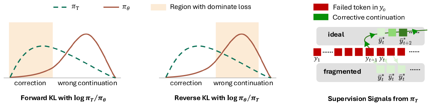
The choice of KL direction interacts with prefix failure asymmetrically. Recovering from $\mathsf{F}(y_{o, <t})$ requires a corrective continuation $\bar{y}^{\star}{\geq t} = (\bar{y}^{\star}t, \bar{y}^{\star}{t+1}, \ldots, \bar{y}^{\star}{t+k-1})$ [^1], generated autoregressively along the correction path, where $\bar{y}^\star_t$ is a correction-onset token ($\bar{y}^\star_t \in {\texttt{Wait}, \texttt{Actually}, \ldots}$) and $\bar{y}^\star_{t+1}, \ldots, \bar{y}^\star_{t+k-1}$ continue the recovery, with $k$ denoting the length of this continuation. Under $\mathsf{F}(y_{o, <t})$, the ideal teacher partially shifts mass from the natural continuation toward $\bar{y}^\star_t$, while the student with high probability remains anchored on the wrong continuation. Forward KL $D(\pi_T | \pi_\theta)$, weighted by $\pi_T$, is dominated by the correction-onset region; its mode-covering nature forces the student onto this out-of-distribution (OOD) mode. This can destabilize training and, in the worst case, lead to mode collapse ([8]). In contrast, reverse KL $D(\pi_\theta | \pi_T)$ is weighted by $\pi_\theta$, so its mode-seeking behavior makes the loss dominated by the wrong-continuation region where the student already places high mass. Since $\pi_\theta(\bar{y}^\star_t)$ is small, the correction signal has limited effect, so updates concentrate on the failing trajectory rather than the recovery tokens.

[^1]: $\bar{y}^{\star}{\geq t}$ is not the literal suffix of $y^\star$, but any correct continuation conditioned on $y{<t}$, i.e., $\operatorname{Verify}(y_{<t} \cdot \bar{y}^{\star}_{\geq t}, , y^\star) = 1$.

Prior work has identified several failure modes of dense token-level KL training and proposed loss-level remedies. These failures are consistent with the prefix-failure mechanism above, even when not explicitly framed this way. Under forward KL, teacher-weighted correction or OOD modes can already dominate the loss, so [8] clip per-token losses to cap unstable high-KL terms. Under reverse KL, the correction mode is instead underweighted by the student-weighted objective; accordingly, [11] use teacher top- $K$ truncation, and [12] reweight losses by entropy and student-teacher disagreement to recover informative teacher-preferred tokens. Thus, these remedies control token-level dominance in opposite directions: clipping suppresses overly dominant forward-KL terms, while truncation or reweighting amplifies underweighted reverse-KL teacher modes. However, all of them leave the failed prefix unchanged.

4.2 Can a Perfect Teacher Recover the Correction Path?

Even granting an ideal teacher, dense per-token KL is structurally limited because it is a post-hoc per-token objective evaluated along the student's rollout. To make this precise, we trace the per-token OPD loss back to its sequence-level origin, which makes the underlying mechanism more transparent. Define the per-token log-ratio $\delta_t !:=! \log \pi_\theta(y_t\mid x, y_{<t}) - \log \pi_T(y_t\mid x, y_{<t})$. Differentiating the sequence-level reverse KL of Equation 1 (full derivation in Appendix A) yields the policy-gradient form

$ \nabla_{\theta} \mathcal{J}(\theta) ;=; \mathbb{E}{\substack{x\sim\mathcal{D}\ y\sim \pi\theta(\cdot\mid x)}} !\left[\sum_{t=1}^{|y|} \bigg(\delta_t ;+; \sum_{t'=t+1}^{|y|} \delta_{t'} \bigg), \nabla_{\theta} \log \pi_\theta(y_t\mid x, y_{<t}) \right], $

where $-\delta_t$ acts as a token-level return. In practice, however, standard OPD implementations ([3, 4]) do not optimize the sequence-level KL in Equation 2; instead, they retain only the immediate log-ratio at each position, yielding the per-token surrogate

$ \nabla_{\theta} \mathcal{J}(\theta) ;=; \mathbb{E}{\substack{x\sim\mathcal{D}\ y\sim \pi\theta(\cdot\mid x)}} !\left[\sum_{t=1}^{|y|} \delta_t \nabla_{\theta} \log \pi_\theta(y_t\mid x, y_{<t}) \right].\tag{3} $

We contrast Equation 3 with the perfect teacher would induce by autoregressively unfolding $\bar{y}^\star_{\geq t}$ along the correction path, delivering the supervision pairs

$ \big{(y_{o, <t}, , \bar{y}^\star_t), ;; \big((y_{o, <t}, \bar{y}^\star_t), , \bar{y}^\star_{t+1}\big), ;; \ldots, ;; \big((y_{o, <t}, \bar{y}^\star_{t:t+k-1}), , \bar{y}^\star_{t+k-1}\big)\big}, $

in which the context grows along the correction path itself. The corresponding ideal gradient is

$ g_{\text{ideal}} ;=; -\sum_{i=1}^{k} \delta_i^{\text{ideal}} \cdot \nabla_\theta \log \pi_\theta!\big(\bar{y}^\star_{t+i-1} , \big|, x, ; y_{o, <t}, , \bar{y}^\star_{t:t+i-1}\big), $

where $\delta_i^{\text{ideal}} := \log \pi_\theta(\bar{y}^\star_{t+i-1} \mid x, y_{o, <t}, \bar{y}^\star_{t:t+i-1}) - \log \pi_T(\bar{y}^\star_{t+i-1} \mid x, y_{o, <t}, \bar{y}^\star_{t:t+i-1})$. Yet under dense KL the contexts are dictated by the frozen student trajectory, not by the unfolding correction. At position $t$, the teacher conveys $\bar{y}^\star_t$ given $y_{o, <t}$, and the student updates its parameters to favor $\bar{y}^\star_t$. At position $t+1$, however, the teacher's supervision is conditioned on $y_{o, <t+1} = (y_{o, <t}, y_{o, t})$ (the original failed trajectory's own continuation), not on the correction path $(y_{o, <t}, \bar{y}^\star_t)$. Because every subsequent prefix the teacher sees is still anchored in the original failure rather than the unfolding correction, the teacher is left repeatedly recommending the same correction-onset token. The supervision pairs delivered to the student therefore form the fragmented sequence

$ \big{(y_{o, <t}, , \bar{y}^\star_t), ;; (y_{o, <t+1}, , \bar{y}^\star_t), ;; \ldots, ;; (y_{o, <t+k-1}, , \bar{y}^\star_t)\big}, $

in which the context grows along the wrong continuation while the target remains stuck at $\bar{y}^\star_t$. The corresponding gradient

$ g_{\text{frag}} ;=; -\sum_{i=0}^{k-1} \delta_i^{\text{frag}} \cdot \nabla_\theta \log \pi_\theta!\big(\bar{y}^\star_t , \big|, x, ; y_{o, <t+i}\big), $

with $\delta_i^{\text{frag}} := \log \pi_\theta(\bar{y}^\star_t \mid x, y_{o, <t+i}) - \log \pi_T(\bar{y}^\star_t \mid x, y_{o, <t+i})$, evaluates the score function at a completely different set of (context, token) pairs than $g_{\text{ideal}}$. The two pair sets share only their first element $(y_{o, <t}, \bar{y}^\star_t)$; beyond it, $g_{\text{ideal}}$ propagates supervision along $(y_{o, <t}, \bar{y}^\star_t, \bar{y}^\star_{t+1}, \ldots)$ while $g_{\text{frag}}$ accumulates supervision along $(y_{o, <t}, y_{o, t}, y_{o, t+1}, \ldots)$. The two trajectories diverge after a single step and never re-intersect:

$ \underbrace{\big{((y_{o, <t}, \bar{y}^\star_{t:t+i-1}), , \bar{y}^\star_{t+i-1})\big}{i=1}^{k}}{\text{required by recovery}} ;;\cap;; \underbrace{\big{(y_{o, <t+i}, , \bar{y}^\star_t)\big}{i=0}^{k-1}}{\text{delivered}} ;=; \big{(y_{o, <t}, , \bar{y}^\star_t)\big}. $

The privileged information $y^\star$ thus stays trapped in per-position marginals. Dense KL keeps recommending $\bar{y}^\star_t$ on ever-deepening wrong-continuation contexts but cannot supervise the multi-step unfolding of $\bar{y}^\star_{\geq t}$, and loss-level interventions only reweight terms within the visited pair set ${(y_{o, <t+i}, \bar{y}^\star_t)}$ rather than move the gradient onto the correction-path pair set. The $g_{\text{frag}}$ signal is not useless, however; biasing the student toward $\bar{y}^\star_t$ can trigger self-correction, though unfolding the full $\bar{y}^\star_{\geq t}$ is bounded by the student's capacity. Our method TRD (Section 5) recovers $g_{\text{ideal}}$ by supervising the per-token KL along a refined trajectory generated by the teacher, so the supervision contexts grow along the correction path itself rather than the frozen failed prefix.

4.3 Experimental Validation of Prefix Failure

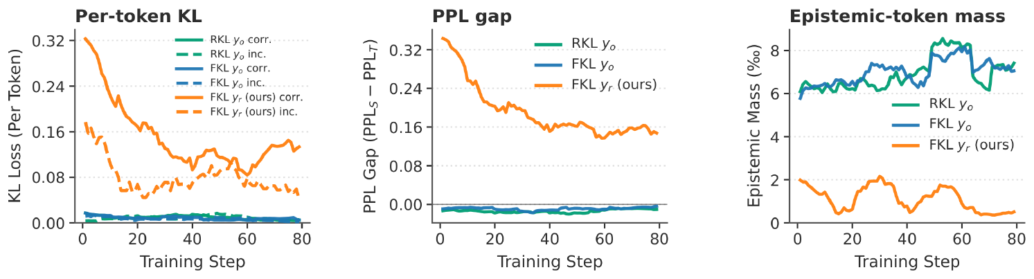
We empirically verify the prefix failure mechanism through three measurements over OPSD training on student rollouts $y_o$ under both forward and reverse KL (Figure 3). A third curve (ours) is included for reference, corresponding to the method introduced in Section 5.

Supervision Degradation (left).

We split the per-token KL between $\pi_T$ and $\pi_S$ by stage-1 verifier outcome (correct vs. incorrect) into token-weighted means $D^{\text{correct}}$ and $D^{\text{incorrect}}$. Both stay pinned near zero on $y_o$, so $\pi_T$ and $\pi_S$ remain aligned and dense KL delivers no signal once $\mathsf{F}(y_{o, <t})$ saturates. Notably, even $D^{\text{incorrect}}$ stays near zero, indicating that the teacher with high probability collapses onto the student's failure rather than diverging to correct it.

Perplexity Gap Shrinkage (middle).

We measure teacher and student perplexities token-wise on the same response mask under teacher-forced decoding, $\mathrm{PPL}S=\exp(-1/|y_o|\sum_t \log\pi_S(y{o, t}\mid y_{o, <t}))$ and $\mathrm{PPL}_T$ defined analogously with $\pi_T$. The gap $\mathrm{PPL}_S-\mathrm{PPL}_T$ stays near zero throughout training, so the privileged condition $y^\star$ delivers essentially vanishing incremental supervision over what the student already represents on its own rollouts.

Epistemic-token Mass Gain (right).

The teacher places $6$ – $8$ textperthousand{} of its per-position mass on $16$ epistemic onset tokens throughout training, matching the $\bar{y}^\star_t$-repeat signature of $g_{\text{frag}}$ predicted in Section 4.2. Strikingly, student and teacher top- $16$ tokens already absorb $97-99$ % of total probability mass ([27], Figure 18), so this allocation commands a disproportionatly dominant share of the remaining $1-3$ % residual budget. The same metric on $y_r$ (ours) collapses below $2$ textperthousand{}, confirming concentration is tied to failed-prefix conditioning rather than a universal teacher property.

5. Trajectory-Refined Distillation

Section Summary: The section introduces Trajectory-Refined Distillation (TRD) to fix a core weakness of standard on-policy distillation: noisy or failed prefixes in student-generated trajectories that ruin later supervision. The method first draws a raw student rollout, then asks the teacher to rewrite it into a refined version that stays anchored to reasoning patterns the student has already shown while correcting errors along the way. The resulting cleaner trajectories are used for the usual distillation loss, simultaneously reducing exposure to bad prefixes and giving the student useful alternative solution paths even when the original rollout was already correct.

The previous section identifies prefix failure as one of the central bottlenecks in OPD. With prefix failure, dense supervision becomes noisy and can even fail to guide the student. Most existing mitigations operate through loss design and leave the offending prefix unchanged. Directly optimizing prefix failure is intractable: whether a prefix has failed is only revealed after the full trajectory is verified, while locating the failure index would require searching $\mathcal{O}(|\mathcal{V}|^k)$ continuations of length $k$. We therefore relax the target to a trajectory-level surrogate that maximizes the expected verifier-pass rate over the dataset $\mathcal{D}$ under the support constraint of $\pi_\theta$:

$ \max q \mathbb{E}{\left(x, y^{\star}\right) \sim \mathcal{D}}\left[\operatorname{Pr}{y \sim q(\cdot \mid x, \cdot)}\left{\operatorname{Verify}\left(y, y^{\star}\right)=1\right}\right] \quad \text s.t.\quad \pi\theta(y \mid x)>0\tag{4} $

We note that this is a trajectory-level distribution support constraint and the optimization objective form mirrors a standard RLVR objective. We emphasize, however, that this objective is not optimized directly in the OPD update; rather, it defines an upstream trajectory-construction task before the standard OPD optimization over $\theta$, namely to construct trajectories that attain higher verifier-pass rates while remaining within the current student's support. These trajectories then serve as the supervision for the subsequent OPD update through the standard distribution-matching loss in Equation 1.

Two extreme choices of $q$ illustrate the tension between objective and constraint. $\textsc{(i)}$ Setting $q(\cdot \mid x, \cdot)=\pi_\theta(\cdot\mid x)$ fails back to standard OPD. The on-policy constraint is satisfied by construction, but this choice fails to mitigate prefix failure beyond current OPD algorithms, since the supervision trajectories are still drawn from $\pi_\theta$. Repeated sampling refines this choice by drawing rollouts and retaining only the verifier-passing ones ([28, 19]), straining inference budgets linearly and yielding nothing on questions the student cannot solve. $\textsc{(ii)}$ Setting $q(\cdot \mid x, \cdot)=\pi^\star$, i.e., the expert policy that produces $y^\star$, attains $\operatorname{Verify}=1$ exactly but generally violates the on-policy support constraint, so this choice falls outside the feasible set and breaks the on-policy character that OPD depends on.

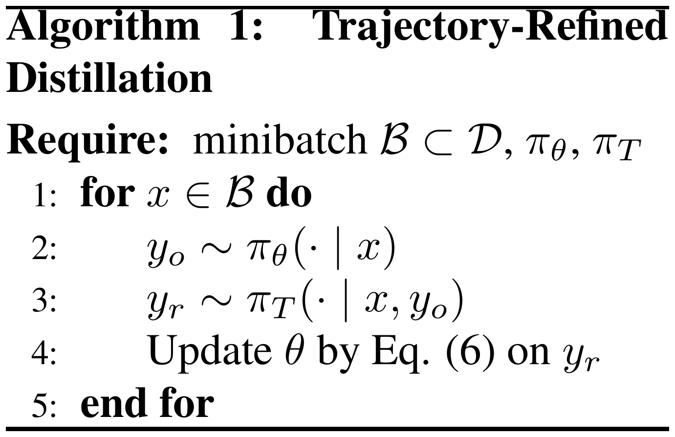
To move beyond the two extremes above, we propose Trajectory-Refined Distillation (TRD), which operates at the trajectory level to optimize Equation 4 by first drawing a raw on-policy rollout $y_o \sim \pi_\theta(\cdot\mid x)$, then asking the teacher to construct a refined trajectory $y_r$ via:

$ y_r \sim q(\cdot\mid x, \cdot);:=;\pi_T(\cdot\mid x, y_o).\tag{5} $

In OPSD, the same backbone implements this teacher query by additionally conditioning on the reference solution $y^*$: $y_r \sim q(\cdot\mid x, \cdot):=\mathrm{sg}[\pi_\theta(\cdot\mid x, y_o, y^*)]$. Crucially, conditioning on $y_o$ anchors $y_r$ to the reasoning patterns $\pi_\theta$ has already demonstrated, i.e., within the policy support, while $\pi_T$ rewrites the erroneous portions to directly mitigate prefix failure. To our knowledge, this is the first trajectory-level optimization design that explicitly targets Equation 4 while respecting the on-policy constraint without prohibitive additional compute overhead. A refined trajectory $y_r$ is then used as supervision for the subsequent OPD update. Per-token KL along $y_r$ reduces exposure to the bimodal teacher mixture (Section 4.1) and recovers the ideal gradient $g_{\text{ideal}}$ (Section 4.2), since supervision contexts grow along the refined trajectory rather than the raw rollout $y_o$ at higher risk of prefix failure.

TRD also boosts the student's exploration beyond standard OPD. On a correct $y_o$, standard OPD provides little new signal: it tends to merely reinforce the high-probability solution path the student already produces due to the fragmented gradient. In contrast, $y_r$ is drawn from $\pi_T(\cdot\mid x, y_o)$ and surfaces alternative valid derivations of the same answer, i.e., paths suggested by the teacher but rarely sampled from $\pi_\theta(\cdot \mid x)$ alone, thereby expanding the set of correct reasoning trajectories the student is supervised on. TRD therefore adds value in both regimes: mitigating failed prefixes when $y_o$ exhibits prefix failure, and broadening the supervision distribution when $y_o$ already succeeds. The training-data analysis in Section 6.5 confirms this (e.g., the correct subset of $y_r$ exhibits a low-length mode absent in $y_o$) and translates into Pass@ $k$ gains in Table 2 and Table 4.

Concretely, given $y_r$, we instantiate the distillation loss as the forward KL with full vocabulary matching over $\mathcal{V}$, which provides mode-covering supervision and stabilizes gradient estimates:

$ \begin{aligned} \mathcal{L}(\theta)

\mathbb{E}{\substack{ x\sim\mathcal{D}\ y_o\sim\pi\theta(\cdot\mid x)\ y_r\sim\pi_T(\cdot\mid x, y_o) }} \left[\frac{1}{|y_r|} \sum_{t=1}^{|y_r|} D\big(\mathrm{sg}!\left[\pi_T(\cdot\mid x, y_o, y_{r, <t}) \right] , \big|, \pi_\theta(\cdot\mid x, y_{r, <t}) \big) \right], \end{aligned}\tag{6} $

The exact prompt template is given in Appendix C.4; Figure 1 (right) and Figure 4 illustrate the full procedure. Figure 3 confirms that these design choices alleviate the issue observed on $y_o$. Beyond the per-token KL recovery on $y_r$ (Left, discussed above), the teacher-student perplexity gap opens on $y_r$ (Middle), restoring the incremental supervision, and the teacher's epistemic onset mass decreases $3$ x less than $y_o$. KL and the PPL gap both decrease steadily as epistemic onset concentration fades, indicating that the teacher signal is genuinely transmitted to the student throughout the training.

6. Experiments

Section Summary: In the experiments, TRD is tested against several standard training baselines on math and code tasks using Qwen3 language models of varying sizes, with evaluations on benchmarks such as AIME24, HMMT25, and LiveCodeBench that measure both average and best-of-16 success rates. Across the OPD and OPSD training regimes, TRD consistently matches or exceeds the base models and other methods by refining entire response trajectories rather than applying token-by-token corrections, leading to the largest gains on harder problems while avoiding capability drops seen in the baselines. The results also highlight that trajectory-level refinement better balances exploration and exploitation during training and produces more reliable outputs at test time.

We evaluate TRD against four dense-KL baselines in both OPD and OPSD settings across math and code benchmarks. We organize the evaluation around three questions. $\textsc{(i)}$ How does TRD perform under the OPD and OPSD settings, and what exploration–exploitation trade-offs emerge (Section 6.2 and Section 6.3)? $\textsc{(ii)}$ Which refinement signal is more effective for TRD under the same student scale (Section 6.4)? $\textsc{(iii)}$ How does refinement change the training trajectories and test-time rollout behavior (Section 6.5)? Full experimental details are given in Appendix C.

6.1 Experiments Setup and Baselines

Models.

We use the Qwen3 model family ([4]). In OPD, the teacher is a separate Qwen3-8B model, and the students are Qwen3-1.7B and Qwen3-4B-Instruct-2507. In OPSD, teacher and student share the same backbone, instantiated by Qwen3-4B-Instruct-2507 and Qwen3-8B, with the teacher distribution induced by privileged conditioning rather than a separate teacher network.

Training Datasets.

For math, we train on the DeepScaleR math corpus ([29]) of roughly 40 thousand problems with solutions; for code, we train on TACO ([30]), an algorithmic code-generation corpus with roughly 25 thousand training problems, with reference solutions and test cases. In OPSD, privileged conditioning uses the dataset reference solution $y^\star$.

Baselines.

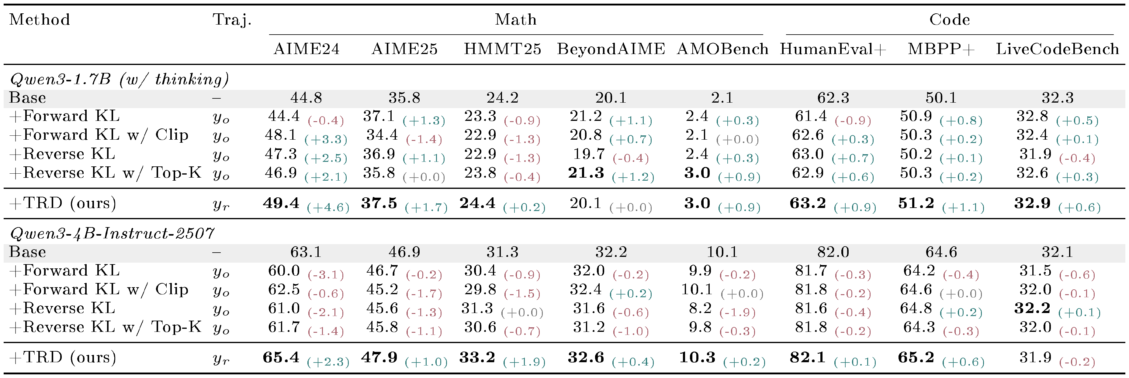
For both OPD and OPSD regimes, we compare against four baselines that train on the raw on-policy rollout $y_o \sim \pi_\theta(\cdot\mid x)$: Forward KL, Forward KL w/ Clip ([8]), Reverse KL, and Reverse KL w/ Top- $K$ ([11]). TRD instead trains on the refined trajectory $y_r$.

Evaluation.

We report Avg@16 and Pass@16 on five math benchmarks, AIME24 ([31]), AIME25 ([32]), HMMT25 ([33]), BeyondAIME ([34]), and AMOBench ([35]). For OPD, we also evaluate code generation on HumanEval+ and MBPP+ ([36]), and LiveCodeBench v6 ([37]). We set the response length $38, 912$ and $16, 384$ for math and code tasks, respectively. For each test question we draw $K{=}16$ completions and grade them with an external verifier; Avg@16 averages the $K$ binary outcomes per question, and Pass@16 is the per-question indicator that at least one of the $K$ samples is correct, both then averaged over the test set.

6.2 OPD Results

::: {caption="Table 1: OPD Avg@16 results (%) using Qwen3-8B as the teacher. Colored subscripts report absolute changes (in %) from the corresponding base model where available; bold marks block best."}

:::

::: {caption="Table 2: OPD Pass@16 results (%) using Qwen3-8B as the teacher. Colored subscripts report absolute changes (in %) from the corresponding base model where available; bold marks block best."}

:::

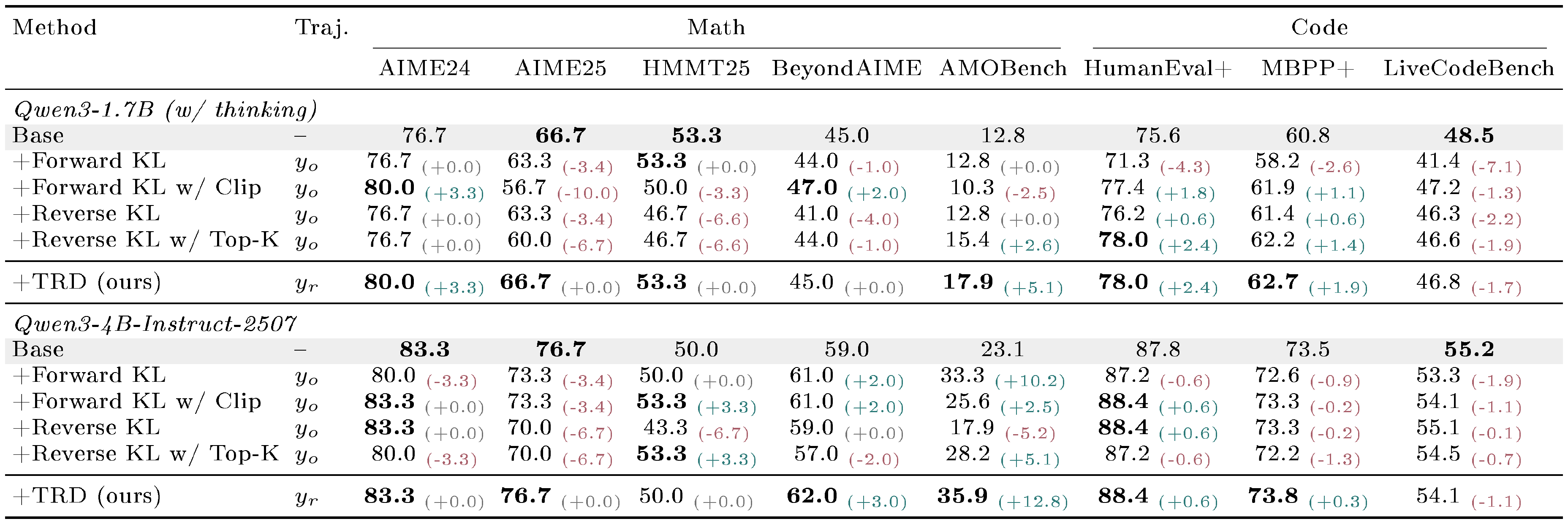
Table 1 reports Avg@16, where TRD improves exploitation over the base model at both student scales and is best or tied-best on seven of eight benchmarks in each block. The gains are largest for the smaller Qwen3-1.7B student, e.g., $+4.6%$ on AIME24. The Qwen3-4B-Instruct-2507 block is more diagnostic: almost all OPD variants trained on $y_o$ fail to match the base model. In contrast, training on $y_r$ preserves the stronger student's base capabilities and turns them into broad gains. This pattern is consistent with the prefix-failure asymmetry in Section 4: token-level pressure toward the teacher can damage the student's existing solution distribution, while trajectory-level refinement provides a safer supervision target.

Table 2 reports Pass@16, where the gains concentrate on harder math benchmarks. TRD gives the best AMOBench result at both scales, improving the base by $+5.1%$ for Qwen3-1.7B and $+12.8%$ for Qwen3-4B-Instruct-2507, while AIME24 and AIME25 are mostly saturated. On code, TRD matches the best HumanEval+ value and is best on MBPP+, but all methods fail to match the base model on LiveCodeBench. For TRD, this suggests that the current teacher may not provide effective refinements on these harder code tasks.

6.3 OPSD Results

::: {caption="Table 3: OPSD Avg@16 results (%). Shared backbone with a privileged teacher. Colored subscripts report absolute changes (in %) from the corresponding base model; bold marks block best."}

:::

::: {caption="Table 4: OPSD Pass@16 results (%). Shared backbone with a privileged teacher. Colored subscripts report absolute changes (in %) from the corresponding base model; bold marks block best."}

:::

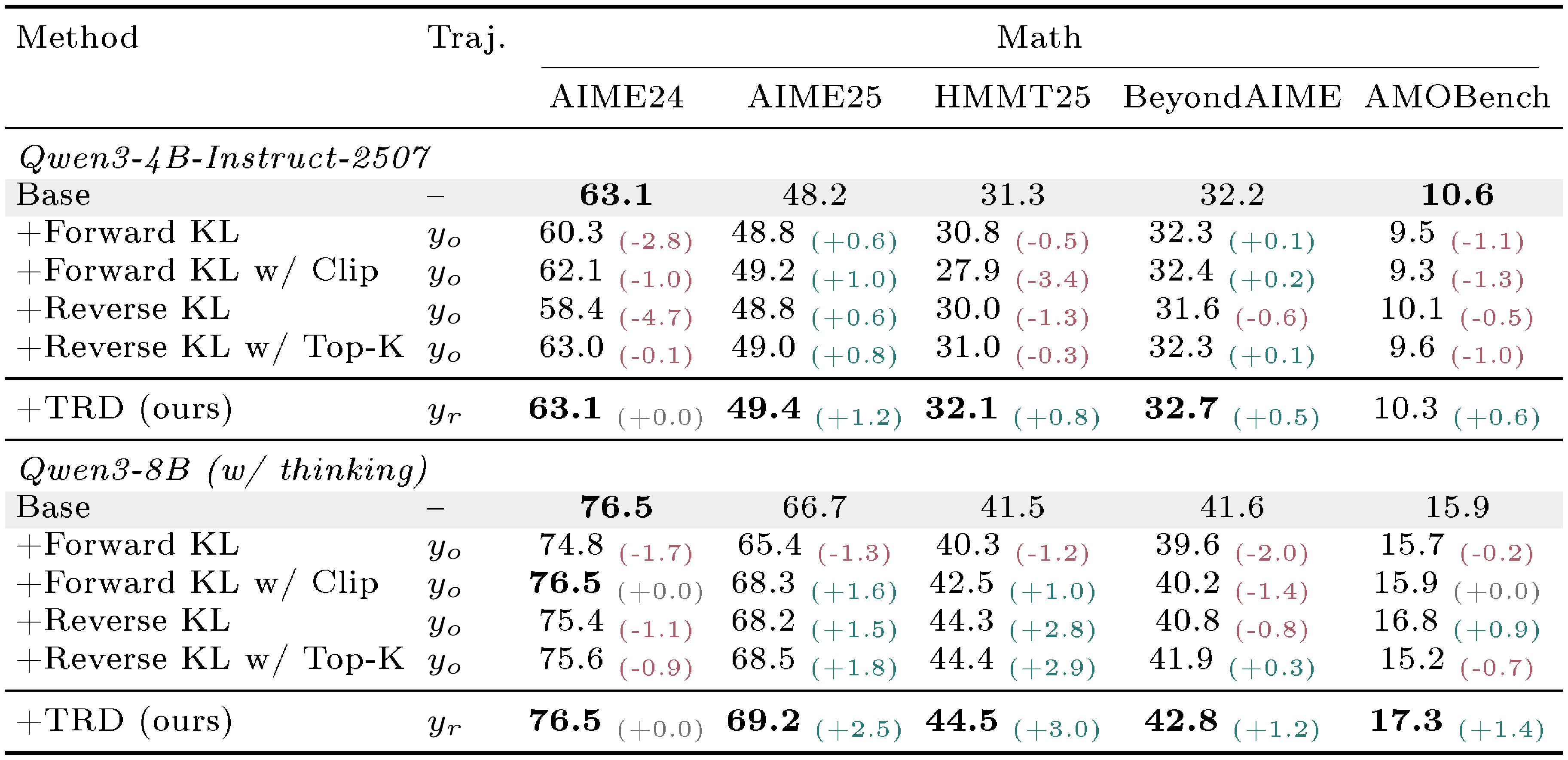
Table 3 reports Avg@16. TRD is best on every benchmark at both scales and never drops below base. AIME24 and AIME25 are largely saturated at this scale (TRD matches base on AIME24, all methods within $\sim!2%$ on AIME25), so the contrast with loss-design baselines is sharpest on the other three benchmarks. Three of four baselines regress on at least one benchmark (e.g., Reverse KL $-5.0%$ on AIME24-4B, Forward KL w/ Clip $-3.4%$ on HMMT25-4B, Forward KL $-2.0%$ on BeyondAIME-8B), reflecting the prefix-failure asymmetry of Section 4, while TRD delivers consistent gains against to other baselines.

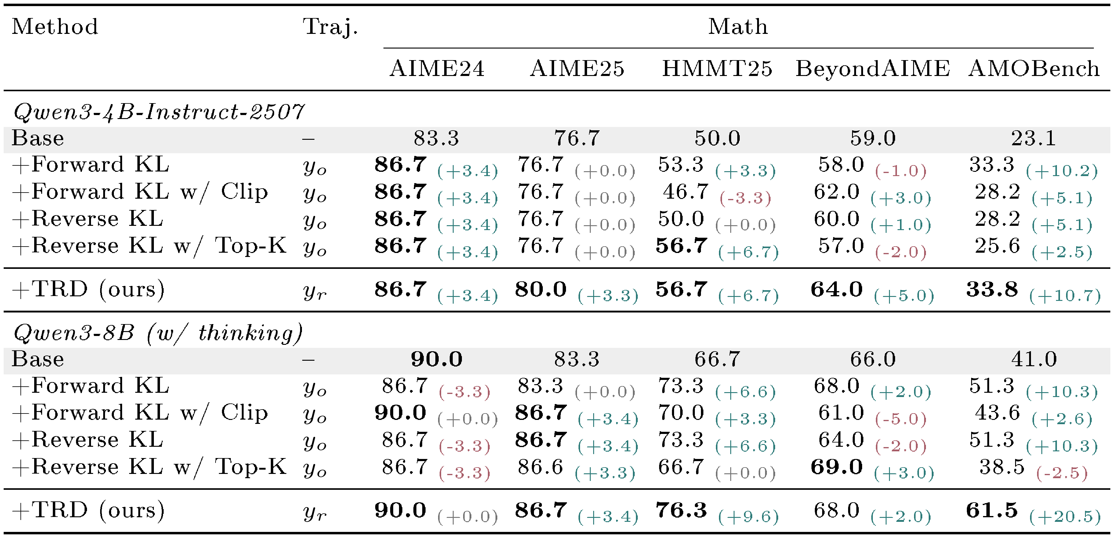
Table 4 reports Pass@16, where TRD's trajectory-level refinement separates most clearly from per-token interventions. The Forward-KL results also reveal a stability–performance trade-off: clipping can improve training stability, but it substantially lags behind the unclipped variant on AMOBench benchmark for both models. On Qwen3-8B, TRD lifts $50%$ relative gain and $15%$ on AMOBench and HMMT25, respectively. The strongest dense-KL baseline on AMOBench stops at $51.3%$ and three of four baselines drop on AIME24. On Qwen3-4B-Instruct-2507, TRD posts $+5.0%$ on BeyondAIME and $+10.7%$ on AMOBench, again top of all baselines.

6.4 Comparing Refinement Signals

::: {caption="Table 5: TRD comparison between OPD and OPSD on Qwen3-4B-Instruct-2507 math benchmarks. Teacher denotes the Qwen3-8B model used as the OPD reference; it is shown only as an upper reference, while bold marks the better value between OPD and OPSD."}

:::

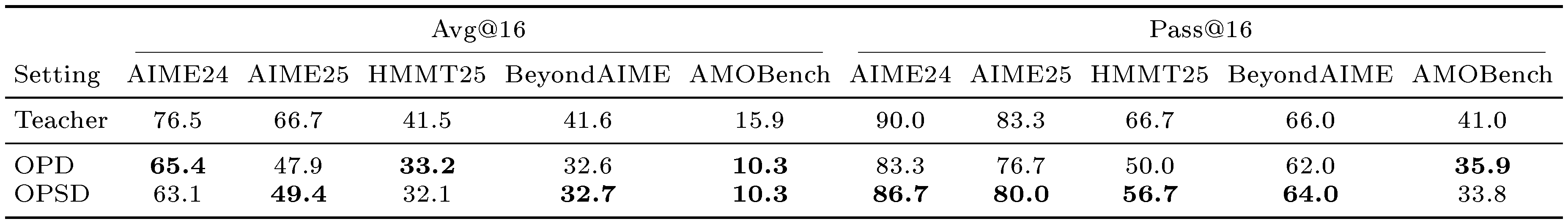
Table 5 collects the relevant results from Table 1, Table 2, Table 3, and Table 4 and compares OPD and OPSD for TRD at the same Qwen3-4B-Instruct scale. Avg@16 is mixed: OPD is stronger on AIME24 and HMMT25, OPSD is stronger on AIME25 and BeyondAIME, and the two tie on AMOBench. Pass@16 is generally stronger under OPSD, which wins on four of five competition-math benchmarks.

The gain suggests that, for optimizing Equation 4, OPSD's privileged information can be more effective than OPD's model scaling: some questions may remain beyond the teacher's ability to refine, while the reference directly supplies the correct solution structure. Using a stronger teacher may reduce such refinement failures, but increases the computational cost of the OPD pipeline. Besides, because OPSD refines with the student backbone conditioned on the reference, it potentially stays closer to the student's support and avoids mismatch between models ([11, 27]).

6.5 Trajectory Analysis

Training Trajectory Analysis ($y_o \text{vs.} y_r$).

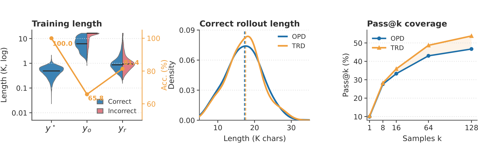
In the OPSD setting, the left panel of Figure 5 contrasts $y^\star$, the raw rollout $y_o$, and the refined trajectory $y_r$ on Qwen3-8B over the training corpus, optimizing Equation 4 indirectly within support. The verifier-pass rate improves from $65.8%$ on $y_o$ to $81.4%$ on $y_r$, and the length distribution compresses by roughly $9\times$ (median $7.7$ K $\to 0.88$ K) toward the reference scale ($y^\star$ median $\sim!0.49$ K). We highlight that the same $\sim!9\times$ compression also applies to the correct half of $y_o$, surfacing a low-length mode in $y_r$ that $y_o$ does not produce. This means even on questions the student already solves, TRD exposes it to alternative, shorter derivations under $y^\star$ guidance, an additional source of supervision diversity; see Appendix B.1 for the full analysis. The same compression also cuts training wall-clock by roughly $60%$ on Qwen3-8B, which offsets the extra $y_r$ sampling cost (Appendix C.3). By supervising on $y_r$ rather than the raw rollout $y_o$, TRD also softens the decaying supervision signals with length inflation ([20, 38, 39]). Appendix B.3 further reports Qwen3-8B corpus-filter ablations by initial-rollout correctness.

Rollout Trajectory Analysis.

We further analyze the AMOBench evaluation rollouts for Qwen3-4B-Instruct-2507 under the OPD regime, comparing vanilla OPD (Forward KL) trained on $y_o$ with TRD trained on $y_r$ under a $K{=}128$ sampling budget. The middle panel of Figure 5 shows the correct-rollout length distribution: the two methods produce highly similar successful-rollout length distributions, while TRD is slightly shorter on average ($18.9$ K $\to$ $18.5$ K characters) with a modest shift of density toward the $18$ – $20$ K range. The right panel shows the complementary coverage view: the gain is modest at $k{=}1$ but widens with the sampling budget, reaching $53.8%$ vs. $46.7%$ at $k{=}128$. Appendix B.2 provides the complementary rollout-trajectory analysis under the OPSD setup.

7. Conclusion

Section Summary: The paper identifies a core flaw in standard on-policy distillation methods called prefix failure, where evaluating the learning signal only along the student model's own outputs creates a mismatched and fragmented training gradient that simpler fixes cannot resolve. To overcome this, it introduces trajectory-level refined distillation (TRD), which generates improved full trajectories with help from privileged information and then applies the training signal along those paths while remaining consistent with the model's own distribution. Experiments show this yields consistent gains on math benchmarks and solves previously unreachable problems, though it adds modest sampling cost and depends on a strong teacher model.

We identify prefix failure as a structural limitation of on-policy (self)-distillation paradigms, where the per-token KL evaluated along the student's frozen rollout induces a bimodal teacher mixture and a fragmented gradient that loss-level fixes leave structurally intact. To address it, we propose TRD, a trajectory-level refinement that draws a refined trajectory $y_r$ under privileged context and supervises the per-token KL along $y_r$, recovering the ideal supervision-pair structure while remaining on-policy. Across five competition-math benchmarks for Qwen3-4B and Qwen3-8B, TRD attains the best Avg@16 on every benchmark and substantial Pass@16 gains, including solving $9/23$ of base-unreachable AMOBench questions and nearly doubling the strongest baseline.

Limitations. First, TRD requires one extra sampling budget to construct $y_r$. This overhead is partially offset by faster KL training on shorter refined trajectories; on Qwen3-8B, the total wall-clock nearly matches the dense-KL baselines (Appendix C.3). Second, TRD relies on the teacher's ability to guide refinement in a way that mitigates prefix failure while keeping the refined trajectories close to the student's on-policy distribution. This limitation is less severe with a stronger teacher that can in principle optimize Equation 4 with promise.

Appendix

Section Summary: The appendix derives the on-policy distillation policy gradient by beginning with a sequence-level reverse KL objective, applying the score-function trick and product rule, then using autoregressive factorization and causality to reduce it to a simple per-token surrogate that matches the standard KL loss. It further presents supporting experiments that analyze training trajectories by comparing raw and refined rollouts on DeepScaleR, break down test-time gains on AMOBench by difficulty, and ablate forward-KL, reverse-KL, and the proposed method under different data filters. All analyses use the on-policy setting with privileged context.

Trajectory-Refined Distillation

A. Derivation of the OPD Policy Gradient

We derive the policy-gradient form Equation 3 of the on-policy distillation gradient, expressing it in the dense form used in our analysis. The derivation parallels [40] and is reproduced here for completeness using the notation of Section 3. Throughout, $\pi_T$ denotes the teacher and $\delta_t !:=! \log \pi_\theta(y_t\mid x, y_{<t}) - \log \pi_T(y_t\mid x, y_{<t})$.

Step 1 (KL as a log-ratio expectation).

Starting from the sequence-level reverse KL $\mathcal{J}(\theta) = \mathbb{E}[D(\pi_\theta(y\mid x), |, \pi_T(y\mid x))]$, the objective expands to

$ \mathcal{J}(\theta) ;=; \mathbb{E}{x\sim\mathcal{D}, , y\sim \pi\theta(\cdot\mid x)} !\big[\log \pi_\theta(y\mid x) - \log \pi_T(y\mid x)\big], $

where the dependence on $\theta$ enters through both the sampling distribution and the integrand.

Step 2 (product rule and score-function trick).

Differentiating under the expectation gives

$ \begin{aligned}\nabla_{\theta}\mathcal{J}(\theta) ;=; \mathbb{E}{x}!\bigg[&\sum_y \big(\nabla{\theta} \pi_\theta(y\mid x)\big)\big(\log \pi_\theta(y\mid x) - \log \pi_T(y\mid x)\big)\&+; \sum_y \pi_\theta(y\mid x), \nabla_{\theta}\log \pi_\theta(y\mid x) \bigg].\end{aligned} $

The second sum vanishes because

$ \sum_y \pi_\theta(y\mid x), \nabla_{\theta}\log \pi_\theta(y\mid x) ;=; \sum_y \nabla_{\theta} \pi_\theta(y\mid x) ;=; \nabla_{\theta} 1 ;=; 0. $

Using $\nabla_{\theta} \pi_\theta = \pi_\theta, \nabla_{\theta}\log \pi_\theta$, the remaining term becomes

$ \nabla_{\theta}\mathcal{J}(\theta) ;=; \mathbb{E}{x\sim\mathcal{D}, , y\sim \pi\theta(\cdot\mid x)} !\big[\big(\log \pi_\theta(y\mid x) - \log \pi_T(y\mid x)\big) \nabla_{\theta}\log \pi_\theta(y\mid x) \big].\tag{7} $

Step 3 (autoregressive decomposition).

Factor $\log \pi_\theta(y\mid x)!=!\sum_{t} \log \pi_\theta(y_{t}\mid x, y_{<t})$ and similarly for $\pi_T$. Equation 7 expands to

$ \mathbb{E}{x, y}!\left[\sum{t=1}^{|y|}\sum_{t'=1}^{|y|} \underbrace{\big(\log \pi_\theta(y_{t'}\mid x, y_{<t'}) - \log \pi_T(y_{t'}\mid x, y_{<t'})\big)}{\delta{t'}}, \nabla_{\theta}\log \pi_\theta(y_t\mid x, y_{<t}) \right]. $

Step 4 (causality, future tokens do not contribute).

For any $t' < t$, $\delta_{t'}$ is measurable with respect to $(x, y_{<t})$, and conditioning on this prefix yields

$ \mathbb{E}{y_t\sim \pi\theta(\cdot\mid x, y_{<t})}!\big[\nabla_{\theta}\log \pi_\theta(y_t\mid x, y_{<t})\big] ;=; \sum_{y_t} \nabla_{\theta} \pi_\theta(y_t\mid x, y_{<t}) ;=; \nabla_{\theta} 1 ;=; 0, $

so all cross terms with $t' < t$ vanish in expectation.

Step 5 (final form).

Retaining only $t' \ge t$ recovers Equation 3,

$ \nabla_{\theta}\mathcal{J}(\theta) ;=; \mathbb{E}{x, y}!\left[\sum{t=1}^{|y|} \Bigg(\sum_{t'=t}^{|y|} \delta_{t'}\Bigg), \nabla_{\theta}\log \pi_\theta(y_t\mid x, y_{<t}) \right]. $

The bracketed quantity $-!\sum_{t' \ge t}!\delta_{t'}$ acts as a return-to-go for token $y_t$. Following common practice ([2, 3]), applying a discount factor of $0$ retains only the term at $t'=t$, which gives the per-token surrogate

$ \nabla_{\theta}\mathcal{J}(\theta) ;\approx; \mathbb{E}{x, y}!\left[\sum{t=1}^{|y|} \big(\log \pi_\theta(y_t\mid x, y_{<t}) - \log \pi_T(y_t\mid x, y_{<t})\big), \nabla_{\theta}\log \pi_\theta(y_t\mid x, y_{<t}) \right], $

which is the gradient of the per-token KL loss in Equation 1, and, with the privileged-context substitution $\pi_T(\cdot\mid x, y_{<t})!=!\pi_\theta(\cdot\mid x, y^\star, y_{<t})$, of the OPSD loss in Equation 2.

B. Additional Experiments

This section provides three complementary analyses beyond the dataset-averaged numbers in Table 1, Table 2, Table 3, and Table 4. Appendix B.1 characterizes the training corpus by comparing $y_o$ and $y_r$ along length, verifier accuracy, and joint outcome on DeepScaleR (Qwen3-4B and Qwen3-8B, with-CoT and without-CoT subsets). Appendix B.2 drills into AMOBench at test time, decomposing Avg@16 and Pass@16 by base-difficulty bucket to localize where TRD's gains arise. Appendix B.3 ablates Forward-KL, Reverse-KL, and TRD under fail, succ, and fail $\to$ succ corpus filters on Qwen3-8B. All ablation studies in this section are conducted under the OPSD setting.

B.1 Training-Trajectory Analysis: $y_o$ vs. $y_r$

Here we inspect the training data on which TRD itself is trained, i.e., the raw rollout $y_o!\sim!\pi_\theta(\cdot\mid x)$ and the refined trajectory $y_r!\sim!\pi_\theta(\cdot\mid x, y_o, y^\star)$ on DeepScaleR. The reference $y^\star$ supplied with each problem comes in two qualities: a small subset ($n{=}4{,}419$) carries a usable reference chain-of-thought, while the rest ($n{=}35{,}826$) carries only a short answer-style reference. We split the analysis along this axis to show that TRD's behavior is consistent across both regimes, reporting Qwen3-4B-Instruct-2507 in Figure 6 and Qwen3-8B in Figure 7, with the with-CoT subset on the top row of each figure and the without-CoT subset on the bottom row. We report numbers as 4B / 8B and as with-CoT / without-CoT when the two subsets diverge.

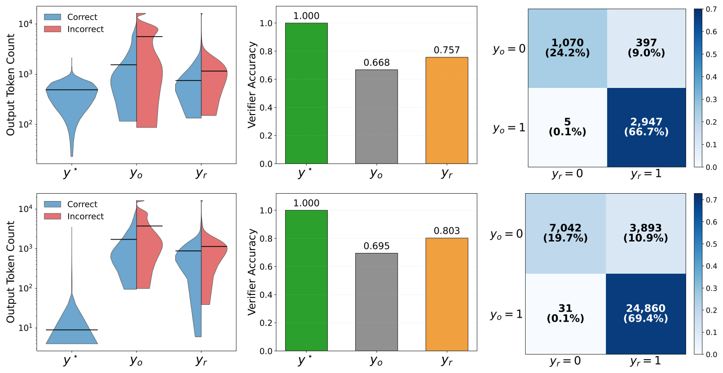
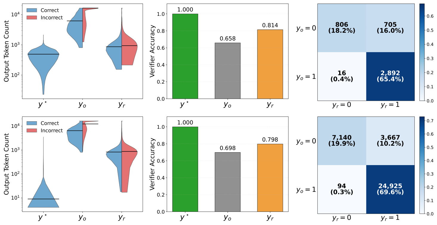
Refinement compresses the trajectory.

The left panels show that $y_r$ moves substantially below $y_o$ in both regimes. With CoT, $y^\star$ has median $\sim!0.49$ K tokens and $y_r$ collapses to $0.85$ K / $0.88$ K from $y_o$ 's $2.2$ K / $7.7$ K (4B / 8B); without CoT, $y^\star$ shrinks to $\sim 9$ tokens (answer-only) and $y_r$ lands at $0.93$ K / $0.83$ K from $y_o$ 's $2.1$ K / $7.5$ K. The compression factor on 8B is similar in both regimes ($\sim!9\times$), confirming that conditioning on $y^\star$ pulls the student toward more concise derivations even when the reference is just a short answer string.

Refinement raises verifier accuracy.

The middle panels report verifier accuracy. With CoT, $y_o$ passes on $66.8%$ / $65.8%$ while $y_r$ passes on $75.7%$ / $81.4%$ ($+8.9%$ / $+15.6%$). Without CoT, $y_o$ passes on $69.5%$ / $69.8%$ and $y_r$ on $80.3%$ / $79.8%$ ($+10.8%$ / $+10.0%$). TRD's training data therefore contains a substantially higher fraction of correct trajectories than what dense-KL baselines train on across both regimes.

Refinement is monotonically corrective.

The right panels decompose the accuracy gap by joint outcome. The fail $\to$ pass to pass $\to$ fail asymmetry is large in every cell ($\sim!80\times$ on 4B-with-CoT, $\sim!44\times$ on 8B-with-CoT, with comparable ratios on the without-CoT subset), consistent with the prefix-failure mechanism in Section 4, i.e., reference-guided refinement primarily corrects dead-end prefixes rather than disturbing already-correct ones. Refinement is not a panacea, around a quarter to a third of $y_o$ failures still survive after refinement and a sub- $1%$ pass $\to$ fail leakage remains in every setting, but the $8$ B runs consistently lift both the recovery rate and absolute accuracy, suggesting the residual fail $\to$ fail mass shrinks as the student grows more capable of producing $y_o$ and consuming $y^\star$.

B.2 Test Rollout Analysis

Setup.

We take the same Qwen3-8B checkpoints used for Table 3 and Table 4 and analyze their test-time rollouts on AMOBench ([35]), the most distillation-sensitive of our five benchmarks (largest absolute Pass@16 gain in Table 4). For each of the $39$ AMOBench questions we draw $K{=}16$ independent completions per method, with the same generation parameters as in Section 6.1 (temperature $0.6$, top- $p!=!0.95$, $38{,}912$-token response budget). Each completion is then $\textsc{(i)}$ tokenized with the Qwen3-8B tokenizer to obtain its output length, and $\textsc{(ii)}$ graded by the AMOBench rule-based verifier. Among the four dense-KL baselines we compare against +Forward KL (no clip), the strongest exploration-side baseline on AMOBench Pass@16 in Table 4.

Base-difficulty buckets.

To isolate where each method helps, we partition the $39$ AMOBench questions by the base model's per-question pass count $b_q := \sum_{i=1}^{16}\operatorname{Verify}(y_q^{(i, \text{base})}, y_q^\star)\in{0, \dots, 16}$ (the number of base-model rollouts that pass the verifier). This yields three difficulty buckets:

• B $0$ ($n=23$): questions on which the base model fails all $16$ attempts. By construction, these are unreachable for the base policy at $K{=}16$ sampling, so any positive Pass@16 in this bucket reflects support expansion rather than sharpening.
• B $1$ – $8$ ($n=12$): medium-difficulty questions the base model solves between $1$ and $8$ times out of $16$, where Avg@16 has the most headroom and sharpening is meaningful.
• B $9$ – $16$ ($n=4$): easy questions the base model already solves at least $9$ times out of $16$, near the saturation ceiling for both Avg@16 and Pass@16.

Bucket sizes are determined by the base model and held fixed when scoring +Forward KL and TRD, so the same question belongs to the same bucket across all three methods.

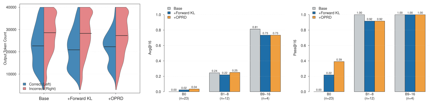
TRD finds shorter solution paths.

The left panel of Figure 8 shows that TRD's correct-rollout distribution is bimodal, with a pronounced low-length mode (around $10^4$ tokens) absent in both Base and +Forward KL, indicating that TRD finds noticeably shorter reasoning chains on the problems it can solve. Incorrect distributions are similar across methods (bunched against the generation cap), so the accuracy gains below come without longer reasoning, i.e., the (accuracy, compute) trade-off moves in the right direction.

Avg@16 by bucket: sharpening on medium difficulty.

The middle panel localizes the per-sample improvement. On B $1$ – $8$, TRD lifts Avg@16 to $0.25$, above both Base ($0.24$) and +Forward KL ($0.22$). The fact that +Forward KL regresses the base model on the same bucket indicates that this sharpening is TRD-specific rather than a generic property of dense-KL distillation. On B $0$, the absolute Avg@16 is small ($0.04$ for TRD vs $0.02$ for +Forward KL), but every positive sample on B $0$ is a trajectory the base policy never produces under $K{=}16$, so TRD's per-sample exploration rate on these questions is roughly twice that of +Forward KL.

Pass@16 by bucket: frontier expansion on hard questions.

The right panel makes the exploration story explicit. On B $0$, the $23$ AMOBench questions where the base model fails on all $16$ attempts, TRD achieves Pass@16 $=0.39$, nearly doubling the strongest baseline (+Forward KL at $0.22$). Because B $0$ questions are by construction unreachable for the base policy at $K{=}16$, any positive Pass@16 here is direct evidence that TRD expands the reachable support of the base policy rather than only sharpening the existing distribution. The mild regression on B $1$ – $8$ Pass@16 ($-1/12$ questions) is overwhelmed by the $+9/23$ gain on B $0$, leaving the dataset-level Pass@16 in Table 4 net positive.

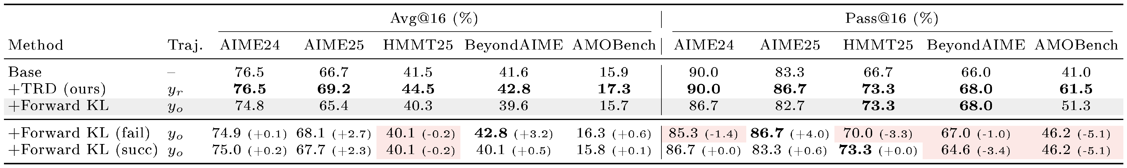
B.3 Ablation: Trajectory-Subset for OPSD on Qwen3-8B

Each table fixes one algorithm and varies the training corpus by filtering on the outcome of $y_o$ and $y_r$. The three subset filters partition $(x, y_o, y_r)$ tuples along the student's verifier outcome on $y_o$. fail keeps tuples where $y_o$ is incorrect ($n{=}12{,}318$), succ keeps those where $y_o$ is correct ($n{=}27{,}927$), and fail $\to$ succ keeps the intersection where $y_o$ is incorrect and $y_r$ is correct ($n{=}4{,}372$). The full corpus is the union $\textit{fail}\cup\textit{succ}$ over $n{=}40{,}245$ DeepScaleR problems and reproduces the no-subset main-table result for each algorithm. Subset rows below the rule report the change relative to the algorithm's no-subset row (e.g., Forward-KL subset rows compare against +Forward KL, not Base).

::: {caption="Table 6: Forward-KL ablation by training subset (Qwen3-8B). Red cells mark drops below that reference; bold marks the column maximum."}

:::

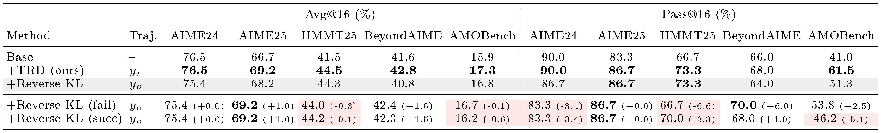
::: {caption="Table 7: Reverse-KL ablation by training subset (Qwen3-8B). Red cells mark drops below that reference; bold marks the column maximum."}

:::

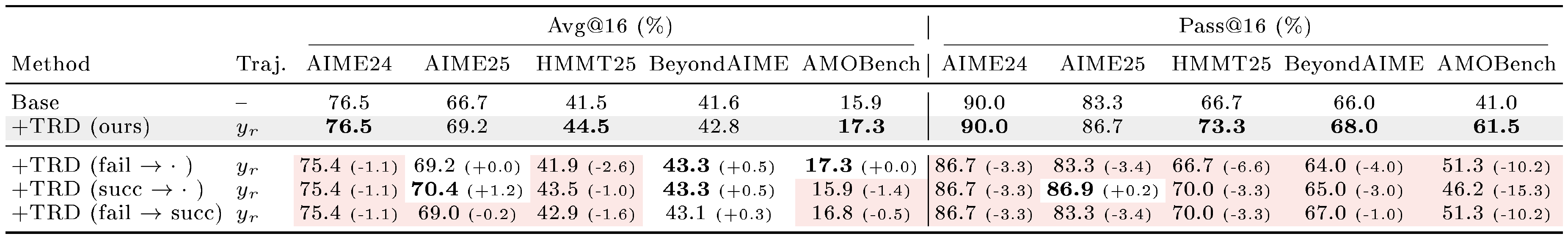
::: {caption="Table 8: TRD ablation by training subset (Qwen3-8B). Red cells mark drops below that reference; bold marks the column maximum."}

:::

Both fail and succ halves are necessary for coverage.

Across Table 6, Table 7, and Table 8, no subset filter is uniformly better than the no-subset corpus for any algorithm. Per-column wins under a filter (e.g., +Forward KL (fail) BeyondAIME Avg@16, +Reverse KL (fail) BeyondAIME Pass@16) are paid for by regressions elsewhere in the same row. Both halves contribute training coverage the per-token KL exploits, so the full corpus is the right default.

Filtering is not an optimization of Equation 6.

Subset filtering changes which trajectories enter $\mathcal{D}$ but not the loss itself, so neither succ-only nor fail-only is an optimization of Equation 6. Each filter also drops a complementary signal. succ-only loses the hard problems on which the student fails unaided, where the teacher provides extra signal that raises the probability of reaching previously unreachable solutions. fail-only loses the alternative-path signal on the easy half, where the teacher can offer stronger or shorter derivations than the student would produce on its own.

Forward KL is the most data-sensitive.

Vanilla +Forward KL regresses Base on four of five Avg@16 benchmarks (AIME24 $-1.7$, AIME25 $-1.3$, HMMT25 $-1.2$, BeyondAIME $-2.0$). Filtering recovers AIME25 (fail $+2.7$, succ $+2.3$) and BeyondAIME (fail $+3.2$), but AIME24 and HMMT25 remain below Base under any filter, and Pass@16 is mostly traded down (AMOBench $-5.1$ under both filters). This column-specific trade is consistent with the mass-spread character of the mode-covering forward KL, which cannot ignore points in the corpus and therefore inherits both the support coverage and the prefix-failure pressure of whichever subset it is fed.

Reverse KL is almost flat under filtering.

Both subset rows sit within $\pm 1.0$ of the no-filter Avg@16 and trade Pass mildly (BeyondAIME up, AMOBench down). The mode-seeking reverse KL already discounts low-probability regions, so removing the fail or succ half does not change the optimization much. This is a stability story, not a quality story, and the no-subset Reverse KL is therefore not noticeably improved by curation.

TRD is hurt by filtering, especially on Pass@16.

Every subset row drops Pass@16 on every benchmark, with double-digit losses on AMOBench ($-10$ to $-15$). Avg@16 deltas are small and mixed. The fail $\to$ succ row ($n{=}4{,}372$, the "ideal" subset where refinement fixed errors) does not outperform full corpus, exhibiting the same Pass losses and no Avg gains worth the data cut. TRD's gain comes from the breadth of the refined corpus rather than from any privileged subset, supporting the choice to train on $y_r$ over the unfiltered corpus by default.

C. Experiment Details

This appendix collects the OPD-first training data and trajectory construction for math and code (Appendix C.1), the math and code evaluation protocols (Appendix C.2), hardware and measured wall-clock budget (Appendix C.3), the shared initial-response prompts and four refinement prompt templates used for OPD/OPSD and math/code (Appendix C.4), the training-metric extraction used in Figure 3 (Appendix C.5), models and OPD/OPSD consistency checks (Appendix C.6), and method-specific and common optimization hyperparameters (Appendix C.7 and Appendix C.8) used throughout Section 6.

C.1 Training Data and Trajectory Construction

Training uses DeepScaleR for math ([29]) and TACO for code ([30]). OPD uses a separate Qwen3-8B teacher; OPSD uses the same backbone as teacher and student, with privileged access to the reference solution $y^\star$.

\begin{tabular}{>{\raggedright\arraybackslash}p{0.22\linewidth}>{\raggedright\arraybackslash}p{0.22\linewidth}>{\raggedright\arraybackslash}p{0.22\linewidth}>{\raggedright\arraybackslash}p{0.22\linewidth}}
\toprule
Setting & Stage 1: $y_o$ & OPD Stage 2: $y_r$ & OPSD Stage 2: $y_r$ \\
\midrule
Samples per problem & $1$ & $1$ & $1$ \\
Temperature & $0.6$ & $0.6$ & $0.6$ \\
Top- $p$ & $0.95$ & $0.95$ & $0.95$ \\
Top- $k$ & $20$ & $20$ & $20$ \\
Prompt budget & Math: $4{,}096$; code: $2{,}048$ tokens & $18{,}432$ tokens & $22{,}528$ tokens \\
Response budget & $16{,}384$ tokens & $16{,}384$ tokens & $16{,}384$ tokens \\
Maximum model length & Math: $20{,}480$; code: $18{,}432$ tokens & $34{,}816$ tokens & $38{,}912$ tokens \\
\bottomrule
\end{tabular}

C.2 Evaluation Protocol

Table 10 summarizes the evaluation configuration. We use $K{=}16$ completions per problem; temperature and response length follow the Qwen3 evaluation setup ([4]).

\begin{tabular}{>{\raggedright\arraybackslash}p{0.22\linewidth}>{\raggedright\arraybackslash}p{0.34\linewidth}>{\raggedright\arraybackslash}p{0.34\linewidth}}
\toprule
Setting & Math evaluation & Code evaluation \\
\midrule
Samples per problem & $K{=}16$ & $K{=}16$ \\
Temperature & $0.6$ & $0.6$ \\
Top- $p$ & $0.95$ & $0.95$ \\
Top- $k$ & $20$ & $20$ \\
Prompt budget & $4{,}096$ tokens & $2{,}048$ tokens \\
Response budget & $38{,}912$ tokens & $16{,}384$ tokens \\
Maximum model length & $43{,}008$ tokens & $18{,}432$ tokens \\
Verifier & rule-based boxed-answer verifier & benchmark unit-test executor \\
\bottomrule
\end{tabular}

Math completions are scored with answer extraction from the final boxed$\ldots$ block. HumanEval+ and MBPP+ are evaluated through EvalPlus; LiveCodeBench uses the lcb_runner code-generation scenario with release version $6$.

Metrics.

For each test question $x_q$ we draw $K{=}16$ independent completions $y_q^{(i)}\sim\pi_\theta(\cdot\mid x_q)$ and score them with a verifier $\operatorname{Verify}(\cdot, \cdot)$: the boxed-answer verifier for math and unit tests for code. Over $N$ test questions,

$ \operatorname{Avg}@K ;=; \frac{1}{N}\sum_{q=1}^{N}\frac{1}{K}\sum_{i=1}^{K}\operatorname{Verify}!\big(y_q^{(i)}, , y_q^\star\big), \quad \operatorname{Pass}@K ;=; \frac{1}{N}\sum_{q=1}^{N}\max_{1\le i\le K}\operatorname{Verify}!\big(y_q^{(i)}, , y_q^\star\big). $

Avg@16 tracks average sample quality; Pass@16 tracks whether at least one of the $16$ samples solves the problem.

Benchmarks.

The math suite contains AIME24/25 ([31, 32]), HMMT25 ([33]), BeyondAIME ([34]), and the $39$ parser-graded AMOBench problems ([35]). The code suite contains HumanEval+, MBPP+ ([36]), and LiveCodeBench v6 ([37]).

C.3 Hardware and Compute

All runs use a single node of $8\times$ H100 80GB GPUs with FSDP2 sharding via verl ([41]). Each row of Table 1, Table 2, Table 3, and Table 4 corresponds to one offline pipeline run, comprising Stage 1 generation, optional Stage 2 generation for $y_r$, one training epoch over the selected parquet, LoRA merge, and post-training evaluation when enabled.

Measured wall-clock.

Table 11 reports the training-pipeline wall-clock by model, setting, and method. The main trade-off is that TRD adds an extra sampling pass to construct $y_r$, but this overhead is partially offset by faster KL training because the refined trajectories are much shorter than $y_o$ (see Appendix B.1). This offset becomes more pronounced as the backbone grows: on Qwen3-8B, TRD and Vanilla OPSD have nearly matched total wall-clock ($9{:}20$ vs. $9{:}40$). Table 12 reports evaluation time separately by model.

\begin{tabular}{>{\raggedright\arraybackslash}p{0.25\linewidth}llcccc}
\toprule
Model & Setting & Method & $y_o$ rollout & $y_r$ rollout & Training & Total \\
\midrule
\multirow{2}{=}{Qwen3-1.7B}
  & \multirow{2}{*}{OPD} & Vanilla OPD & $3{:}30$ & -- & $1{:}10$ & $4{:}40$ \\
  & & TRD & $3{:}30$ & $4{:}00$ & $0{:}40$ & $8{:}10$ \\
\midrule
\multirow{4}{=}{Qwen3-4B-Instruct-2507}
  & \multirow{2}{*}{OPD} & Vanilla OPD & $4{:}00$ & -- & $1{:}20$ & $5{:}20$ \\
  & & TRD & $4{:}00$ & $4{:}00$ & $1{:}00$ & $9{:}00$ \\
\cmidrule(lr){2-7}
  & \multirow{2}{*}{OPSD} & Vanilla OPSD & $2{:}10$ & -- & $2{:}10$ & $4{:}20$ \\
  & & TRD & $2{:}10$ & $2{:}00$ & $1{:}20$ & $5{:}30$ \\
\midrule
\multirow{2}{=}{Qwen3-8B}
  & \multirow{2}{*}{OPSD} & Vanilla OPSD & $4{:}20$ & -- & $5{:}20$ & $9{:}40$ \\
  & & TRD & $4{:}20$ & $2{:}50$ & $2{:}10$ & $9{:}20$ \\
\bottomrule
\end{tabular}

\begin{tabular}{lcc}
\toprule
Model & Math suite & Code suite \\
\midrule
Qwen3-1.7B & $2{:}00$ & $6{:}30$ \\
Qwen3-4B-Instruct-2507 & $2{:}00$ & $3{:}00$ \\
Qwen3-8B & $4{:}00$ & -- \\
\bottomrule
\end{tabular}

C.4 Initial and Refinement Prompts

Stage-1 initial-response prompts are task-specific but shared by OPD and OPSD. They produce the raw rollout $y_o$ used by the dense-KL baselines and by the Stage-2 refinement prompts. The refinement prompt is also task-specific and differs between OPD and OPSD only in whether the reference solution $y^\star$ is shown. OPD refinement uses the separate teacher and hides $y^\star$; OPSD refinement uses the shared model under privileged conditioning and includes $y^\star$.

Math Initial Response.

Code Initial Response.

OPD Math Refinement.

OPSD Math Refinement.

OPD Code Refinement.

OPSD Code Refinement.

C.5 Training Metrics for Figure 3

The diagnostic curves in Figure 3 are collected in the OPSD setting, because that setting controls for teacher–student model mismatch. The same trainer can log these metrics for OPD, but the reported OPD direct-variant runs keep them off unless explicitly enabled. For the OPSD diagnostic runs, we log three quantities, all computed on student rollouts $y_o\sim\pi_\theta(\cdot\mid x)$ over response tokens (with mask $m_{i, t}\in{0, 1}$). All three are first accumulated as numerator/denominator within each step, then divided, so the reported value is a token-weighted mean.

Per-token KL by rollout outcome.

Each prompt $x_i$ carries a binary stage-1 outcome label $b_i$, set to $1$ (correct) if the base model's stage-1 rollout passes the verifier and to $0$ (incorrect) otherwise. The per-token KL between teacher and student is averaged separately within each bucket,

$ D^{\text{correct}} ;=; \frac{\sum_{i:, b_i=1}\sum_t D_{\mathrm{KL}, i, t}, m_{i, t}}{\sum_{i:, b_i=1}\sum_t m_{i, t}}, \qquad D^{\text{incorrect}} ;=; \frac{\sum_{i:, b_i=0}\sum_t D_{\mathrm{KL}, i, t}, m_{i, t}}{\sum_{i:, b_i=0}\sum_t m_{i, t}}, $

where $D_{\mathrm{KL}, i, t}$ is the per-token KL term in Equation 2. The values are directly comparable to the global $D$ since both use a token-weighted denominator.

Epistemic-token mass.

Let $\mathcal{E}\subset\mathcal{V}$ be the set of epistemic onset tokens. We construct $\mathcal{E}$ from $16$ phrases,

Wait, Actually, However, Alternatively, Oops, Wrong, Error, Incorrect, Correction, Sorry, Hmm, Oh, Hold, Pause, Uh, Um, by tokenising each phrase under the student tokenizer in two variants (bare string and leading-space) and collecting the first sub-word id, then deduplicating. At each response position $(i, t)$ we measure how much teacher mass falls on $\mathcal{E}$ before any KL temperature scaling,

$ \mathrm{mass}{i, t} ;=; \sum{v\in\mathcal{E}} \pi_T(v\mid x_i, y^\star_i, y_{<t}) ;=; \sum_{v\in\mathcal{E}} \mathrm{softmax}!\big(\boldsymbol{\ell}^{T}_{i, t}\big)_v, $

and report the token-weighted mean $\big(\sum_{i, t} \mathrm{mass}{i, t}, m{i, t}\big)\big/\big(\sum_{i, t} m_{i, t}\big)$. The metric is computed only on the full-vocabulary path (i.e., when teacher logits are materialised) and is independent of the KL-loss temperature.

Teacher-student perplexity gap.

Both perplexities are token-weighted under teacher-forced decoding on the same response mask,

$ \mathrm{PPL}S ;=; \exp!\Bigg(\frac{\sum{i, t} -\log \pi_S(y_{i, t}\mid y_{<t}), m_{i, t}}{\sum_{i, t} m_{i, t}}\Bigg), \qquad \mathrm{PPL}T ;=; \exp!\Bigg(\frac{\sum{i, t} -\log \pi_T(y_{i, t}\mid y_{<t}), m_{i, t}}{\sum_{i, t} m_{i, t}}\Bigg). $

Since both share the same mask and use $T{=}1$ log-probabilities, the gap $\mathrm{PPL}_S-\mathrm{PPL}_T$ is directly comparable across runs.

C.6 Models and Distillation Setup

OPD uses a frozen separate Qwen3-8B teacher and Qwen3-1.7B or Qwen3-4B-Instruct-2507 students ([4]). The teacher branch is never updated and its logits are detached before KL computation. OPSD uses Qwen3-4B-Instruct-2507 and Qwen3-8B as shared teacher/student backbones: the same base model produces privileged teacher logits under reference-solution conditioning, while LoRA adapters update only the student branch.

Across OPD and OPSD we keep the implementation matched wherever possible: both use the same math/code corpora, prompt adapters, Stage-1 rollout sampler, full-vocabulary KL implementation, optimizer, LoRA configuration, FSDP2 execution path, and evaluation sampling parameters. The intended differences are limited to (i) teacher identity, separate Qwen3-8B for OPD versus same-backbone privileged conditioning for OPSD; (ii) whether $y^\star$ is visible to the teacher/refinement prompt; (iii) the longer OPSD prompt budgets needed to include $y^\star$; and (iv) the clipping constant in the canonical clipped-forward recipes, where OPD direct wrappers named clip01 set $c{=}0.1$ while the OPSD canonical wrapper sets $c{=}0.06$. Code evaluation is reported for OPD direct variants; OPSD remains the math shared-backbone control unless a code row is explicitly added.

We apply LoRA of rank $r{=}64$, scaling $\alpha{=}128$, dropout $0.05$, on all attention and MLP linear layers (q_proj, k_proj, v_proj, o_proj, gate_proj, up_proj, down_proj). After training we merge the adapters into the base weights before evaluation.

C.7 Method-Specific Hyperparameters

Table 13 lists settings that distinguish the direct OPD/OPSD rows. All rows use full-vocabulary KL over the Qwen3 vocabulary ($|\mathcal{V}|!\approx!152$ K), temperature $T{=}1.0$, AdamW, bfloat16, gradient checkpointing, one trainer epoch per update, and LoRA rank $64$ / alpha $128$. On one $8$-GPU node the default per-GPU batch is $1$ and gradient accumulation is $16$, giving effective batch $128$ unless a launch script explicitly overrides it.

```latextable {caption="Table 13: Per-method direct-variant settings. OPD direct clipped-forward wrappers named clip01 use c=0.1; the canonical OPSD clipped-forward wrapper uses c=0.06. Max-length columns are training-time model lengths for teacher-forced KL."} \begin{tabular}{lcccccc} \toprule Method & Traj. & KL dir. & Clip $c$ & Top- $K$ & Teacher prompt & OPD / OPSD max len. \ \midrule Forward KL & $y_o$ & forward & $0$ & -- & vanilla & $18{,}432$ / $22{,}528$ \ Forward KL w/ Clip & $y_o$ & forward & $0.1$ OPD, $0.06$ OPSD & -- & vanilla & $18{,}432$ / $22{,}528$ \ Reverse KL & $y_o$ & reverse & $0$ & -- & vanilla & $18{,}432$ / $22{,}528$ \ Reverse KL w/ Top- $K$ & $y_o$ & reverse & $0$ & $32$ & vanilla & $18{,}432$ / $22{,}528$ \ TRD (ours) & $y_r$ & forward & $0$ & -- & refine & $34{,}816$ / $38{,}912$ \ \bottomrule \end{tabular}

#### C.8 Common Optimization Hyperparameters

Settings shared across the current direct-variant recipes are listed in Table 14.

```latextable {caption="Table 14: Common optimization and generation hyperparameters used by the direct OPD/OPSD recipes unless a launch script explicitly overrides them."}
\begin{tabular}{ll}
\toprule
Setting & Value \\
\midrule
Optimizer & AdamW ($\beta_1{=}0.9$, $\beta_2{=}0.999$, $\epsilon{=}10^{-8}$) \\
Peak learning rate & $5\!\times\!10^{-6}$ \\
Precision & bfloat16 \\
Gradient checkpointing & enabled \\
Per-GPU train batch & $1$ \\
Gradient accumulation & $16$ \\
Gradient clipping & $1.0$ \\
LR schedule & linear warmup, cosine decay to $0.1\!\times$ peak LR \\
Warmup ratio & $0.1$ \\
Weight decay & $0.005$ \\
Epochs per update & $1$ \\
Full-vocab KL chunk size & $512$ tokens \\
LoRA save/merge & save adapter checkpoints and merge before evaluation \\
Sequence packing & remove-padding via verl FSDP2 \\
Sequence parallel & ulysses, size $1$ \\
Rollout generation & temperature $0.6$, top- $p{=}0.95$, top- $k{=}-1$, max sequences $64$ \\
Code evaluation & temperature $0.6$, top- $p{=}0.95$, max sequences $128$ \\
\bottomrule
\end{tabular}

Loss formulation.

For each method, the per-token KL is computed in full vocabulary at temperature $T$ as

$ D^{(T)}\big(p, |, q\big) ;=; \sum_{v\in\mathcal{V}} p_T(v), \big(\log p_T(v) - \log q_T(v)\big), $

with $p_T(v) \propto \exp(\ell_v / T)$. The clipping baseline applies a per-token cap $\min(D_{\mathrm{KL}, t}, c)$ before averaging over the response mask; OPD direct clip01 rows use $c{=}0.1$ and OPSD canonical clipped-forward rows use $c{=}0.06$. Top- $K$ replaces $\mathcal{V}$ by the teacher's top- $32$ support $\mathcal{S}_t$ and renormalizes both $p_T$ and $q_T$ to sum to $1$ on $\mathcal{S}_t$ before evaluating $D$.

References

Section Summary: This section compiles a lengthy list of academic citations, primarily recent arXiv preprints and conference papers from 2024–2026 on knowledge distillation methods for large language models, with a strong emphasis on on-policy and self-distillation techniques. It also incorporates foundational works, technical reports on specific AI models, and resources such as math and coding benchmarks used to evaluate model performance. The entries reflect ongoing research trends in reinforcement learning and efficient model training.

[1] Gu et al. (2024). MiniLLM: Knowledge Distillation of Large Language Models. In The Twelfth International Conference on Learning Representations (ICLR). https://openreview.net/forum?id=5h0qf7IBZZ. arXiv:2306.08543.

[2] Agarwal et al. (2024). On-policy distillation of language models: Learning from self-generated mistakes. In The twelfth international conference on learning representations.

[3] Lu, Kevin and Thinking Machines Lab (2025). On-Policy Distillation. Thinking Machines Lab: Connectionism. https://thinkingmachines.ai/blog/on-policy-distillation. doi:10.64434/tml.20251026.

[4] Yang et al. (2025). Qwen3 technical report. arXiv preprint arXiv:2505.09388.

[5] DeepSeek-AI (2026). DeepSeek-V4: Towards Highly Efficient Million-Token Context Intelligence. https://huggingface.co/deepseek-ai/DeepSeek-V4-Pro.

[6] Xiao et al. (2026). Mimo-v2-flash technical report. arXiv preprint arXiv:2601.02780.

[7] Zeng et al. (2026). Glm-5: from vibe coding to agentic engineering. arXiv preprint arXiv:2602.15763.

[8] Zhao et al. (2026). Self-Distilled Reasoner: On-Policy Self-Distillation for Large Language Models. arXiv preprint arXiv:2601.18734. arXiv:2601.18734.

[9] Hübotter et al. (2026). Reinforcement Learning via Self-Distillation. arXiv preprint arXiv:2601.20802.

[10] Shenfeld et al. (2026). Self-Distillation Enables Continual Learning. arXiv preprint arXiv:2601.19897.

[11] Fu et al. (2026). Revisiting On-Policy Distillation: Empirical Failure Modes and Simple Fixes. arXiv preprint arXiv:2603.25562.

[12] Xu et al. (2026). TIP: Token Importance in On-Policy Distillation. arXiv preprint arXiv:2604.14084.

[13] Hinton et al. (2015). Distilling the knowledge in a neural network. arXiv preprint arXiv:1503.02531.

[14] Song, Mingyang and Zheng, Mao (2026). A Survey of On-Policy Distillation for Large Language Models. arXiv preprint arXiv:2604.00626.

[15] Shi et al. (2026). Experiential reinforcement learning. arXiv preprint arXiv:2602.13949.

[16] Ye et al. (2026). On-policy context distillation for language models. arXiv preprint arXiv:2602.12275.

[17] Penaloza et al. (2026). Privileged Information Distillation for Language Models. arXiv preprint arXiv:2602.04942.

[18] Wang et al. (2026). Skill-SD: Skill-Conditioned Self-Distillation for Multi-turn LLM Agents. arXiv preprint arXiv:2604.10674.

[19] Alex Stein et al. (2026). GATES: Self-Distillation under Privileged Context with Consensus Gating. https://arxiv.org/abs/2602.20574. arXiv:2602.20574.

[20] Feng Luo et al. (2026). Demystifying OPD: Length Inflation and Stabilization Strategies for Large Language Models. https://arxiv.org/abs/2604.08527. arXiv:2604.08527.

[21] Chenxu Yang et al. (2026). Self-Distilled RLVR. https://arxiv.org/abs/2604.03128. arXiv:2604.03128.

[22] Kim et al. (2026). Why Does Self-Distillation (Sometimes) Degrade the Reasoning Capability of LLMs?. arXiv preprint arXiv:2603.24472.

[23] Gengsheng Li et al. (2026). Unifying Group-Relative and Self-Distillation Policy Optimization via Sample Routing. https://arxiv.org/abs/2604.02288. arXiv:2604.02288.

[24] Yuanda Xu et al. (2026). PACED: Distillation and On-Policy Self-Distillation at the Frontier of Student Competence. https://arxiv.org/abs/2603.11178. arXiv:2603.11178.

[25] Jin et al. (2026). Entropy-Aware On-Policy Distillation of Language Models. arXiv preprint arXiv:2603.07079.

[26] Jang et al. (2026). Stable On-Policy Distillation through Adaptive Target Reformulation. arXiv preprint arXiv:2601.07155.

[27] Li et al. (2026). Rethinking On-Policy Distillation of Large Language Models: Phenomenology, Mechanism, and Recipe. arXiv preprint arXiv:2604.13016.

[28] Brown et al. (2024). Large language monkeys: Scaling inference compute with repeated sampling. arXiv preprint arXiv:2407.21787.

[29] Luo et al. (2025). Deepscaler: Surpassing o1-preview with a 1.5 b model by scaling rl. Notion Blog. 3(5).

[30] Li et al. (2023). TACO: Topics in Algorithmic COde Generation Dataset. arXiv preprint arXiv:2312.14852.

[31] AI-MO (2024). AIME 2024. https://huggingface.co/datasets/AI-MO/aimo-validation-aime.

[32] OpenCompass (2025). AIME 2025. https://huggingface.co/datasets/opencompass/AIME2025.

[33] HMMT (2025). Harvard-MIT Mathematics Tournament, February 2025. https://www.hmmt.org/www/archive/results.

[34] ByteDance Seed (2025). Seed1.5-Thinking: Advancing Superb Reasoning Models with Reinforcement Learning. https://huggingface.co/datasets/ByteDance-Seed/BeyondAIME.

[35] An et al. (2025). Amo-bench: Large language models still struggle in high school math competitions. arXiv preprint arXiv:2510.26768.

[36] Liu et al. (2023). Is Your Code Generated by ChatGPT Really Correct? Rigorous Evaluation of Large Language Models for Code Generation. In Thirty-seventh Conference on Neural Information Processing Systems. https://openreview.net/forum?id=1qvx610Cu7.

[37] Jain et al. (2024). LiveCodeBench: Holistic and Contamination Free Evaluation of Large Language Models for Code. arXiv preprint arXiv:2403.07974.

[38] Liu et al. (2026). Prefix Teach, Suffix Fade: Local Teachability Collapse in Strong-to-Weak On-Policy Distillation. arXiv preprint arXiv:2605.13643.

[39] Ziheng et al. (2026). Less is More: Early Stopping Rollout for On-Policy Distillation. arXiv preprint arXiv:2605.27028.

[40] Yang et al. (2026). Learning beyond Teacher: Generalized On-Policy Distillation with Reward Extrapolation. arXiv preprint arXiv:2602.12125.

[41] Sheng et al. (2024). HybridFlow: A Flexible and Efficient RLHF Framework. arXiv preprint arXiv:2409.19256.