Byte Latent Transformer: Patches Scale Better Than Tokens
Show me an executive summary.
Purpose and context
Large language models today rely on tokenization—a fixed preprocessing step that groups bytes into tokens from a static vocabulary. This approach creates problems: models struggle with noisy input, lack understanding of how words are spelled, perform poorly on low-resource languages, and cannot flexibly adjust how much computation they spend on different parts of text. Previous attempts to train models directly on bytes failed to match tokenized models at scale because processing every byte individually was prohibitively expensive.
This work introduces the Byte Latent Transformer (BLT), a new architecture that processes raw bytes without tokenization while matching or exceeding the performance of state-of-the-art tokenized models like Llama 3. The key innovation is dynamic patching: the model groups bytes into variable-length patches based on how difficult the next byte is to predict, allocating more computation where the text is complex and less where it is predictable.
Approach
BLT uses three components: a lightweight encoder that converts bytes to patch representations, a large transformer that processes patches, and a lightweight decoder that converts patches back to bytes. Unlike tokenization, which uses fixed groupings determined before training, BLT segments bytes dynamically using entropy—a measure of prediction difficulty—from a small auxiliary language model. High-entropy positions start new patches, meaning the model spends more computation on unpredictable content (like the first word of a sentence) and less on predictable content (like common word endings).
We trained BLT models ranging from 400 million to 8 billion parameters on up to 4 trillion bytes of text and code. We compared these against Llama 2 and Llama 3 models trained with identical computational budgets, measuring both training efficiency and downstream task performance on reasoning, coding, translation, and robustness benchmarks.
Main findings
BLT matches the training efficiency of Llama 3 at all scales tested, up to 8 billion parameters. This is the first demonstration that byte-level models can compete with tokenization at this scale. More importantly, BLT offers a new efficiency trade-off: by using larger average patch sizes (grouping more bytes per patch), the model can reduce inference computation by up to 50% with only minor performance loss. For example, a patch size of 6 bytes instead of 4.5 reduces inference cost substantially while maintaining competitive accuracy.
BLT also unlocks a new scaling dimension. In tokenized models, a fixed inference budget determines model size—you cannot grow the model without spending more at inference. BLT can simultaneously increase both model size and patch size while keeping inference cost constant, because larger patches mean fewer expensive transformer steps. Our experiments show this simultaneous scaling produces better performance trends than simply scaling tokenized models.
On robustness and character-level tasks, BLT significantly outperforms tokenized models. When we introduce character-level noise (random capitalization, dropped letters, repeated characters), BLT maintains accuracy 8 points higher on average than Llama 3 trained on the same data. On tasks requiring spelling manipulation or phonetic understanding, BLT achieves 25+ point improvements over Llama 3.1, despite being trained on 16 times less data. For low-resource language translation, BLT shows consistent improvements, particularly on languages with non-Latin scripts where tokenization performs poorly.
We also demonstrated that existing tokenized models can be converted to BLT by initializing the large transformer with pretrained Llama weights and training only the byte-level components. This "bytefying" approach produces models with improved robustness while reducing the training needed to reach strong performance.
What this means
These results show that tokenization is not necessary for state-of-the-art language model performance. BLT provides three concrete advantages: (1) reduced inference cost through larger patches without sacrificing training efficiency, (2) better scaling properties by growing model size within a fixed inference budget, and (3) substantially improved robustness to input variations and better handling of rare words, character-level reasoning, and multilingual content.
The inference cost reduction matters for deployment at scale. A 50% reduction in computation per response translates directly to lower server costs and faster response times. The robustness improvements address real operational concerns: models that break when users make typos or use unusual formatting are less reliable in production.
The ability to scale model size while holding inference cost constant changes the trade-off for model development. Organizations can invest more in training to get better models without increasing deployment costs, or they can maintain current performance levels while reducing inference expenses.
Recommendations and next steps
For teams building new language models: consider BLT architecture instead of tokenization, especially if inference cost or robustness to input variation are concerns. The code is publicly available for implementation.
For teams with existing tokenized models: explore the "bytefying" approach to improve robustness, particularly for applications involving noisy user input, multilingual content, or tasks requiring character-level understanding. This requires less training than building from scratch.
For further development: the current work uses scaling laws derived for tokenized models, which may not be optimal for BLT. Calculating BLT-specific scaling laws could reveal better parameter-to-data ratios. Additionally, learning the patching scheme end-to-end during training (rather than using a separate entropy model) may improve performance further.
Limitations and confidence
These experiments used training regimes optimized for tokenized models (Llama 3 scaling laws), which may not be optimal for BLT. Actual optimal training could produce even better results. The implementation is not yet as optimized as mature tokenization-based systems, so wall-clock training time may be slower despite theoretical computational equivalence. The bytefying experiments (converting Llama 3 to BLT) show promise but need more work to fully match the original model's performance across all tasks.
We have high confidence that BLT matches tokenized models on training efficiency and substantially improves robustness and character-level understanding. The inference cost reductions are well-established. The scaling trends showing advantages from simultaneous model and patch size growth are robust across two computational budgets and multiple model sizes, but have only been tested up to 8 billion parameters.
Artidoro Pagnoni, Ram Pasunuru‡^{\ddagger}‡, Pedro Rodriguez‡^{\ddagger}‡, John Nguyen‡^{\ddagger}‡, Benjamin Muller, Margaret Li1,⋄^{1,\diamond}1,⋄, Chunting Zhou⋄^{\diamond}⋄, Lili Yu, Jason Weston, Luke Zettlemoyer, Gargi Ghosh, Mike Lewis, Ari Holtzman†,2,⋄^{\dagger,2,\diamond}†,2,⋄, Srinivasan Iyer†^{\dagger}†
FAIR at Meta
1^{1}1 Paul G. Allen School of Computer Science & Engineering, University of Washington
2^{2}2 University of Chicago
‡^{\ddagger}‡ Joint second author
†^{\dagger}† Joint last author
⋄^{\diamond}⋄ Work done at Meta
Abstract
We introduce the Byte Latent Transformer (BLT\text{B{\scriptsize LT}}BLT), a new byte-level LLM architecture that, for the first time, matches tokenization-based LLM performance at scale with significant improvements in inference efficiency and robustness. BLT\text{B{\scriptsize LT}}BLT encodes bytes into dynamically sized patches, which serve as the primary units of computation. Patches are segmented based on the entropy of the next byte, allocating more compute and model capacity where increased data complexity demands it. We present the first fLOP\text{f{\scriptsize LOP}}fLOP controlled scaling study of byte-level models up to 8B parameters and 4T training bytes. Our results demonstrate the feasibility of scaling models trained on raw bytes without a fixed vocabulary. Both training and inference efficiency improve due to dynamically selecting long patches when data is predictable, along with qualitative improvements on reasoning and long tail generalization. Overall, for fixed inference costs, BLT\text{B{\scriptsize LT}}BLT shows significantly better scaling than tokenization-based models, by simultaneously growing both patch and model size.
1. Introduction
In this section, the authors introduce the Byte Latent Transformer (BLT), a new architecture that processes raw bytes without tokenization while matching the performance of traditional tokenization-based language models at scale. The central problem is that existing large language models rely on tokenization—a heuristic preprocessing step that introduces biases, domain sensitivity, noise vulnerability, and multilingual inequity—yet training directly on bytes has been prohibitively expensive due to long sequence lengths. BLT addresses this by dynamically grouping bytes into variable-length patches based on next-byte entropy, allocating more compute to complex, high-entropy predictions and less to predictable sequences. The architecture comprises a large global transformer operating on patches and two lightweight local models for encoding and decoding bytes. Through the first FLOP-controlled scaling study of byte-level models up to 8B parameters, BLT achieves training parity with Llama 3 while reducing inference costs by up to 50%, demonstrates superior robustness to input noise, and unlocks a new scaling dimension where model size can increase while maintaining fixed inference budgets.
We introduce the Byte Latent Transformer (BLT), a tokenizer-free architecture that learns from raw byte data and, for the first time, matches the performance of tokenization-based models at scale, with significant improvements in efficiency and robustness (§ 6). Existing large language models (lLM\text{l{\scriptsize LM}}lLM s) are trained almost entirely end-to-end, except for tokenization—a heuristic pre-processing step that groups bytes into a static set of tokens. Such tokens bias how a string is compressed, leading to shortcomings such as domain/modality sensitivity ([1]), sensitivity to input noise (§ 6), a lack of orthographic knowledge ([2]), and multilingual inequity ([3, 4, 5]).
Tokenization has previously been essential because directly training lLM\text{l{\scriptsize LM}}lLM s on bytes is prohibitively costly at scale due to long sequence lengths ([6]). Prior works mitigate this by employing more efficient self-attention ([7, 8]) or attention-free architectures ([9]) (§ 8). However, this primarily helps train small models. At scale, the computational cost of a Transformer is dominated by large feed-forward network layers that run on every byte, not the cost of the attention mechanism.
To efficiently allocate compute, we propose a dynamic, learnable method for grouping bytes into patches (§ 2) and a new model architecture that mixes byte and patch information. Unlike tokenization, BLT\text{B{\scriptsize LT}}BLT has no fixed vocabulary for patches. Arbitrary groups of bytes are mapped to latent patch representations via light-weight learned encoder and decoder modules. We show that this results in more efficient allocation of compute than tokenization-based models.
Tokenization-based lLM\text{l{\scriptsize LM}}lLM s allocate the same amount of compute to every token. This trades efficiency for performance, since tokens are induced with compression heuristics that are not always correlated with the complexity of predictions. Central to our architecture is the idea that models should dynamically allocate compute where it is needed. For example, a large transformer is not needed to predict the ending of most words, since these are comparably easy, low-entropy decisions compared to choosing the first word of a new sentence. This is reflected in BLT\text{B{\scriptsize LT}}BLT 's architecture (§ 3) where there are three transformer blocks: two small byte-level local models and a large global latent transformer (Figure 2). To determine how to group bytes into patches and therefore how to dynamically allocate compute, BLT\text{B{\scriptsize LT}}BLT segments data based on the entropy of the next-byte prediction creating contextualized groupings of bytes with relatively uniform information density.
We present the first fLOP\text{f{\scriptsize LOP}}fLOP-controlled scaling study of byte-level models up to 8B parameters and 4T training bytes, showing that we can train a model end-to-end at scale from bytes without fixed-vocabulary tokenization. Overall, BLT\text{B{\scriptsize LT}}BLT matches training fLOP\text{f{\scriptsize LOP}}fLOP-controlled performance of Llama 3 while using up to 50% fewer fLOP\text{f{\scriptsize LOP}}fLOP s at inference (§ 5). We also show that directly working with raw bytes provides significant improvements in modeling the long-tail of the data. BLT\text{B{\scriptsize LT}}BLT models are more robust than tokenizer-based models to noisy inputs and display enhanced character level understanding abilities demonstrated on orthographic knowledge, phonology, and low-resource machine translation tasks (§ 6). Finally, with BLT\text{B{\scriptsize LT}}BLT models, we can simultaneously increase model size and patch size while maintaining the same inference fLOP\text{f{\scriptsize LOP}}fLOP budget. Longer patch sizes, on average, save compute which can be reallocated to grow the size of the global latent transformer, because it is run less often. We conduct inference- fLOP\text{f{\scriptsize LOP}}fLOP controlled scaling experiments (Figure 1), and observe significantly better scaling trends than with tokenization-based architectures.
In summary, this paper makes the following contributions: 1) We introduce
BLT\text{B{\scriptsize LT}}BLT, a byte latent
lLM\text{l{\scriptsize LM}}lLM architecture that dynamically allocates compute to improve
fLOP\text{f{\scriptsize LOP}}fLOP efficiency, 2) We show that we achieve training
fLOP\text{f{\scriptsize LOP}}fLOP-controlled parity with Llama 3 up to 8B scale while having the option to trade minor losses in evaluation metrics for
fLOP\text{f{\scriptsize LOP}}fLOP efficiency gains of up to 50%, 3)
BLT\text{B{\scriptsize LT}}BLT models unlock a new dimension for scaling
lLM\text{l{\scriptsize LM}}lLM s, where model size can now be scaled while maintaining a fixed-inference budget, 4) We demonstrate the improved robustness of
BLT\text{B{\scriptsize LT}}BLT models to input noise and their awareness of sub-word aspects of input data that token-based
lLM\text{l{\scriptsize LM}}lLM s miss. We release the training and inference code for
BLT\text{B{\scriptsize LT}}BLT at
https://github.com/facebookresearch/blt.
2. Patching: From Individual Bytes to Groups of Bytes
In this section, the authors introduce patching as a method to group bytes into variable-length segments that serve as computational units in BLT, directly addressing the inefficiency of processing individual bytes. They present three patching approaches: strided patching groups bytes into fixed-size chunks but wastes compute on easy predictions and splits words inconsistently; space patching creates boundaries at whitespace, naturally aligning with linguistic units but lacking flexibility across languages and domains; and entropy patching, their proposed solution, uses predictions from a small byte-level language model to identify high-uncertainty byte positions as patch boundaries, either through a global entropy threshold or by detecting entropy increases that break monotonic decreases within patches. Unlike BPE tokenization, which uses a fixed vocabulary and cannot segment incrementally during generation, entropy patching dynamically allocates compute where complexity demands it while satisfying the incremental patching property—ensuring patch boundaries depend only on preceding bytes, not future context.
Segmenting bytes into patches allows BLT\text{B{\scriptsize LT}}BLT to dynamically allocate compute based on context. Figure 3 shows several different methods for segmenting bytes into patches. Formally, a patching function fpf_pfp segments a sequence of bytes x={xi,∣i=1,…n}\pmb{x}=\{x_i, |i=1, \ldots n\}x={xi,∣i=1,…n} of length nnn into a sequence of m<nm < nm<n patches p={pj∣j=1,…,m}\pmb{p}=\{p_j|j=1, \ldots, m\}p={pj∣j=1,…,m} by mapping each xix_ixi to the set 0, 1 where 1 indicates the start of a new patch. For both token-based and patch-based models, the computational cost of processing data is primarily determined by the number of steps executed by the main Transformer. In BLT\text{B{\scriptsize LT}}BLT, this is the number of patches needed to encode the data with a given patching function. Consequently, the average size of a patch, or simply patch size, is the main factor for determining the cost of processing data during both training and inference with a given patching function (§ 4.5). Next, we introduce three patching functions: patching with a fixed number of bytes per patch (§ 2.1), whitespace patching (§ 2.2), and dynamically patching with entropies from a small byte lM\text{l{\scriptsize M}}lM (§ 2.3). Finally, we discuss incremental patching and how tokenization is different from patching (§ 2.4).
2.1 Strided Patching Every K Bytes
Perhaps the most straightforward way to group bytes is into patches of fixed size kkk as done in MegaByte ([10]). The fixed stride is easy to implement for training and inference, provides a straightforward mechanism for changing the average patch size, and therefore makes it easy to control the fLOP\text{f{\scriptsize LOP}}fLOP cost. However, this patching function comes with significant downsides. First, compute is not dynamically allocated to where it is needed most: one could be either wasting a transformer step jjj if only predicting whitespace in code, or not allocating sufficient compute for bytes dense with information such as math. Second, this leads to inconsistent and non-contextual patching of similar byte sequences, such as the same word being split differently.
2.2 Space Patching
[12] proposes a simple yet effective improvement over strided patching that creates new patches after any space-like bytes which are natural boundaries for linguistic units in many languages. In Space patching, a latent transformer step (i.e., more fLOP\text{f{\scriptsize LOP}}fLOP s) is allocated to model every word. This ensures words are patched in the same way across sequences and that flops are allocated for hard predictions which often follow spaces. For example, predicting the first byte of the answer to the question "Who composed the Magic Flute? ‾\underline{ } " is much harder than predicting the remaining bytes after "M" since the first character significantly reduces the number of likely choices, making the completion "Mozart" comparatively easy to predict. However, space patching cannot gracefully handle all languages and domains, and most importantly cannot vary the patch size. Next, we introduce a new patching method that uses the insight that the first bytes in words are typically most difficult to predict, but that provides a natural mechanism for controlling patch size.
2.3 Entropy Patching: Using Next-Byte Entropies from a Small Byte LM
Rather than relying on a rule-based heuristic such as whitespace, we instead take a data-driven approach to identify high uncertainty next-byte predictions. We introduce entropy patching, which uses entropy estimates to derive patch boundaries.
We train a small byte-level auto-regressive language model on the training data for BLT\text{B{\scriptsize LT}}BLT and compute next byte entropies under the LM distribution pep_{e}pe over the byte vocabulary V\mathcal{V}V:
We experiment with two methods to identify patch boundaries given entropies H(xi)H(x_i)H(xi). The first, finds points above a global entropy threshold, as illustrated in Figure 4. The second, identifies points that are high relative to the previous entropy. The second approach can also be interpreted as identifying points that break approximate monotonically decreasing entropy withing the patch.
Patch boundaries are identified during a lightweight preprocessing step executed during dataloading. This is different from [13] where classifier is trained to predict entropy-based patch boundaries. In our experiments (§ 4), we compare these two methods for distinguishing between low and high entropy bytes.
2.4 The Byte-Pair Encoding (BPE) Tokenizer and Incremental Patching
Many modern lLM\text{l{\scriptsize LM}}lLM s, including our baseline Llama 3, use a subword tokenizer like bPE\text{b{\scriptsize PE}}bPE ([14, 15]). We use "tokens" to refer to byte-groups drawn from a finite vocabulary determined prior to training as opposed to "patches" which refer to dynamically grouped sequences without a fixed vocabulary. A critical difference between patches and tokens is that with tokens, the model has no direct access to the underlying byte features.
A crucial improvement of BLT\text{B{\scriptsize LT}}BLT over tokenization-based models is that redefines the trade off between the vocabulary size and compute. In standard lLM\text{l{\scriptsize LM}}lLM s, increasing the size of the vocabulary means larger tokens on average and therefore fewer steps for the model but also larger output dimension for the final projection layer of the model. This trade off effectively leaves little room for tokenization based approaches to achieve significant variations in token size and inference cost. For example, Llama 3 increases the average token size from 3.7 to 4.4 bytes at the cost of increasing the size of its embedding table 4x compared to Llama 2.
When generating, BLT\text{B{\scriptsize LT}}BLT needs to decide whether the current step in the byte sequence is at a patch boundary or not as this determines whether more compute is invoked via the Latent Transformer. This decision needs to occur independently of the rest of the sequence which has yet to be generated. Thus patching cannot assume access to future bytes in order to choose how to segment the byte sequence. Formally, a patching scheme fpf_pfp satisfies the property of incremental patching if it satisfies:
bPE\text{b{\scriptsize PE}}bPE is not an incremental patching scheme as the same prefix can be tokenized differently depending on the continuation sequence, and therefore does not satisfy the property above.
3. BLT\text{B{\scriptsize LT}}BLT Architecture
BLT\text{B{\scriptsize LT}}BLT is composed of a large global autoregressive language model that operates on patch representations, along with two smaller local models that encode sequences of bytes into patches and decode patch representations back into bytes (Figure 2).
3.1 Latent Global Transformer Model
The Latent Global Transformer is an autoregressive transformer model G\mathcal{G}G with lGl_{\mathcal{G}}lG layers, which maps a sequence of latent input patch representations, pjp_jpj into a sequence of output patch representations, ojo_joj. Throughout the paper, we use the subscript jjj to denote patches and iii to denote bytes. The global model uses a block-causal attention mask ([11]), which restricts attention to be up to and including the current patch within the current document. This model consumes the bulk of the fLOP\text{f{\scriptsize LOP}}fLOP s during pre-training as well as inference, and thus, choosing when to invoke it allows us to control and vary the amount of compute expended for different portions of the input and output as a function of input/output complexity.
3.2 Local Encoder
The Local Encoder Model, denoted by E\mathcal{E}E, is a lightweight transformer-based model with lE<<lGl_{\mathcal{E}} << l_{\mathcal{G}}lE<<lG layers, whose main role is to efficiently map a sequence of input bytes bib_ibi, into expressive patch representations, pjp_jpj. A primary departure from the transformer architecture is the addition of a cross-attention layer after each transformer layer, whose function is to pool byte representations into patch representations (Figure 5). First, the input sequence of bytes, bib_ibi, are embedded using a R256×hE\mathbb{R}^{256 \times h_{\mathcal{E}}}R256×hE matrix, denoted as xix_ixi. These embeddings are then optionally augmented with additional information in the form of hash-embeddings (§ 3.2.1). A series of alternating transformer and cross-attention layers (§ 3.2.2) then transform these representations into patch representations, pip_ipi that are processed by the global transformer, G\mathcal{G}G. The transformer layers use a local block causal attention mask; each byte attends to a fixed window of wEw_{\mathcal{E}}wE preceding bytes that in general can cross the dynamic patch boundaries but can not cross document boundaries. The following subsections describe details about the embeddings and the cross-attention block.
3.2.1 Encoder Hash n-gram Embeddings
A key component in creating robust, expressive representations at each step iii is to incorporate information about the preceding bytes. In BLT\text{B{\scriptsize LT}}BLT, we achieve this by modeling both the byte bib_ibi individually and as part of a byte n-gram. For each step iii, we first construct byte-grams
for each byte position iii and nnn from three to eight.
We then introduce hash nnn-gram embeddings, that map all byte nnn-grams via a hash function to an index in an embedding table EnhashE_{n}^{hash}Enhash with a fixed size, for each size n∈{3,4,5,6,7,8}n \in\{3, 4, 5, 6, 7, 8\}n∈{3,4,5,6,7,8} ([16]). The resulting embedding is then added to the embedding of the byte before being normalized and passed as input to the local encoder model. We calculate the augmented embedding
We normalize eie_iei by the number of nnn-grams sizes plus one and use RollPolyHash as defined in Appendix C. In Section 7, we ablate the effects of nnn-gram hash embeddings with different values for nnn and embedding table size on fLOP\text{f{\scriptsize LOP}}fLOP-controlled scaling law trends. In addition to hash nnn-gram embeddings, we also experimented with frequency based nnn-gram embeddings, and we provide details of this exploration in Appendix D.
3.2.2 Encoder Multi-Headed Cross-Attention
We closely follow the input cross-attention module of the Perceiver architecture ([17]), with the main difference being that latent representations correspond to variable patch representations as opposed to a fixed set of latent representations (Figure 5), and only attend to the bytes that make up the respective patch. The module comprises a query vector, corresponding to each patch pjp_jpj, which is initialized by pooling the byte representations corresponding to patch pjp_jpj, followed by a linear projection, EC∈RhE×(hE×UE)\mathcal{E}_{C} \in \mathbb{R}^{h_{\mathcal{E}} \times (h_{\mathcal{E}} \times U_{\mathcal{E}})}EC∈RhE×(hE×UE), where UEU_{\mathcal{E}}UE is the number of encoder cross-attention heads. Formally, if we let fbytes(pj)f_{\text{bytes}}(p_j)fbytes(pj) denote the sequence of bytes corresponding to patch, pjp_jpj, then we calculate
where P∈Rnp×hGP \in \mathbb{R}^{n_p \times h_{\mathcal{G}}}P∈Rnp×hG represents npn_pnp patch representations to be processed by the global model, which is initialized by pooling together the byte embeddings eie_iei corresponding to each patch pjp_jpj. WqW_qWq, WkW_kWk, WvW_vWv and WoW_oWo are the projections corresponding to the queries, keys, values, and output where the keys and values are projections of byte representations hih_ihi from the previous layer (eie_iei for the first layer). We use a masking strategy specific to patching where each query QjQ_jQj only attends to the keys and values that correspond to the bytes in patch jjj. Because we use multi-headed attention over Q,KQ, KQ,K and VVV and patch representations are typically of larger dimension (hGh_{\mathcal{G}}hG) than hEh_{\mathcal{E}}hE, we maintain PlP_lPl as multiple heads of dimension hEh_{\mathcal{E}}hE when doing cross-attention, and later, concat these representations into hGh_{\mathcal{G}}hG dimensions. Additionally, we use a pre-LayerNorm on the queries, keys and values and no positional embeddings are used in this cross-attention module. Finally, we use a residual connection around the cross-attention block.
3.3 Local Decoder
Similar to the local encoder, the local decoder D\mathcal{D}D is a lightweight transformer-based model with lD<<lGl_{\mathcal{D}} << l_{\mathcal{G}}lD<<lG layers, that decodes a sequence of global patch representations ojo_joj, into raw bytes, yiy_iyi. The local decoder predicts a sequence of raw bytes, as a function of previously decoded bytes, and thus, takes as input the hidden representations produced by the local encoder for the byte-sequence. It applies a series of lDl_{\mathcal{D}}lD alternating layers of cross attention and transformer layers. The cross-attention layer in the decoder is applied before the transformer layer to first create byte representations from the patch representations, and the local decoder transformer layer operates on the resulting byte sequence.
3.3.1 Decoder Multi-headed Cross-Attention
In the decoder cross-attention, the roles of the queries and key/values are interchanged i.e. the byte-representations are now the queries, and the patch representations are now the key/values. The initial byte-representations for the cross-attention are initialized as the byte embeddings from the last encoder layer i.e. hlEh_{l_{\mathcal{E}}}hlE. The subsequent byte-representations for layer lll, dl,id_{l, i}dl,i are computed as:
where once again, Wk,WvW_k, W_vWk,Wv are key/value projection matrices that operate on a linear transformation and split operation DC\mathcal{D}_CDC, applied to the final patch representations ojo_joj from the global model, WqW_qWq is a query projection matrices operating on byte representations dl−1d_{l-1}dl−1 from the previous decoder transformer layer (or hlEh_{l_{\mathcal{E}}}hlE for the first layer), and WoW_oWo is the output projection matrix, thus making B∈RhD×nbB \in \mathbb{R}^{h_{\mathcal{D}} \times n_b}B∈RhD×nb, where nbn_bnb is the number of output bytes. The next decoder representations DlD_lDl are computed using a decoder transformer layer on the output of the cross-attention block, BBB. As in the local encoder cross-attention, we use multiple heads in the attention, use pre LayerNorms, no positional embeddings, and a residual connection around the cross-attention module.
4. Experimental Setup
In this section, the authors establish a rigorous experimental framework to ensure fair comparison between BLT and tokenization-based models by controlling for context length and compute budgets. They train models on two datasets: the 2 trillion token Llama 2 dataset for scaling law experiments and a new 1 trillion token BLT-1T dataset for downstream evaluation. A key innovation is entropy-based patching, which uses a 100M parameter byte-level language model to identify high-uncertainty positions as patch boundaries, with thresholds calibrated to achieve target patch sizes while maintaining constant batch sizes in bytes rather than tokens. The setup equalizes context by reducing sequence length for larger patch sizes, ensuring all models process the same average number of bytes per batch. Training employs standard Llama 3 architectural choices including SwiGLU activations, RoPE embeddings, and AdamW optimization with a learning rate of 4e-4, chosen through hyperparameter search to be optimal for both BLT and token-based models across different scales.
In this section, the authors provide technical details and supplementary analyses for the BLT architecture. Model hyperparameters are specified across different scales from 400M to 8B parameters, showing the encoder uses just one layer while the global transformer and decoder scale differently. FLOP computation equations are formalized for both standard transformers and BLT models, accounting for attention, feed-forward operations, and cross-attention mechanisms unique to BLT. The rolling polynomial hash function is defined mathematically for n-gram embeddings. An ablation study compares frequency-based versus hash-based n-gram embeddings, finding that hash-based approaches perform better as they avoid vocabulary limitations of frequency tables. Finally, a visual example demonstrates how entropy-based patching operates on MMLU few-shot examples, revealing that repeated phrases get consolidated into larger patches during inference, thereby reducing computational load while potentially affecting reasoning performance, which motivates the use of entropy resets and monotonicity constraints.
We carefully design controlled experiments to compare BLT\text{B{\scriptsize LT}}BLT with tokenization based models with particular attention to not give BLT\text{B{\scriptsize LT}}BLT any advantages from possibly using longer sequence contexts.
4.1 Pre-training Datasets
All model scales that we experiment in this paper are pre-trained on two datasets: 1) The Llama 2 dataset ([18]), which comprises 2 trillion tokens collected from a variety of publicly available sources, which are subsequently cleaned and filtered to improve quality; and 2) BLT\text{B{\scriptsize LT}}BLT-1T: A new dataset with 1 trillion tokens gathered from various public sources, and also including a subset of the pre-training data released by Datacomp-LM ([19]). The former is used for scaling law experiments on optimal number of tokens as determined by [11] to determine the best architectural choices for BLT\text{B{\scriptsize LT}}BLT, while the latter is used for a complete pre-training run to compare with Llama 3 on downstream tasks. Neither of these datasets include any data gathered from Meta products or services. Furthermore, for baseline experiments for tokenizer-based models, we use the Llama 3 tokenizer with a vocabulary size of 128K tokens, which produced stronger baseline performance that the Llama 2 tokenizer in our experiments.
4.2 Entropy Model
The entropy model in our experiments is a byte level language model trained on the same training distribution as the full BLT\text{B{\scriptsize LT}}BLT model. Unless otherwise mentioned, we use a transformer with 100M parameters, 14 layers, and a hidden dimensionality of 512, and sliding window attention of 512 bytes. The remaining hyperparameters are the same as in our local and global transformers. We experimented with different model sizes, receptive fields, and architectures as discussed in Section 7. In particular, when the receptive field of the model is small enough, the trained entropy model can be encoded in an efficient lookup table.
4.3 Entropy Threshold and Equalizing Context Length
For models using entropy-based patching, we estimate a patching threshold that achieves a desired average patch size on the pretraining data mix. In BLT\text{B{\scriptsize LT}}BLT, unlike with tokenization, the patch size can be arbitrarily chosen having significant implications on the context size used by the model. To maintain the same average context length and avoid giving larger patch sizes unfair advantage, we ensure that the number of bytes in each batch remains constant in expectation. This means that we reduce the sequence length of models with larger patch sizes. On Llama 2 data, we use a 8k byte context while on the BLT\text{B{\scriptsize LT}}BLT-1T dataset we increase the context to 16k bytes on average while maintaining the same batch size of 16M bytes on average.
While the average batch size is constant, when loading batches of data, dynamic patching methods yield different ratios of bytes to patches. For efficiency reasons, our implementation of BLT\text{B{\scriptsize LT}}BLT training packs batches of patches to avoid padding steps in the more expensive latent transformer. This ensures that every batch has the same number of patches. During training we pad and possibly truncate byte sequences to 12k and 24k bytes respectively for Llama 2 and BLT\text{B{\scriptsize LT}}BLT-1T datasets, to avoid memory spikes from sequences with unusually large patches.
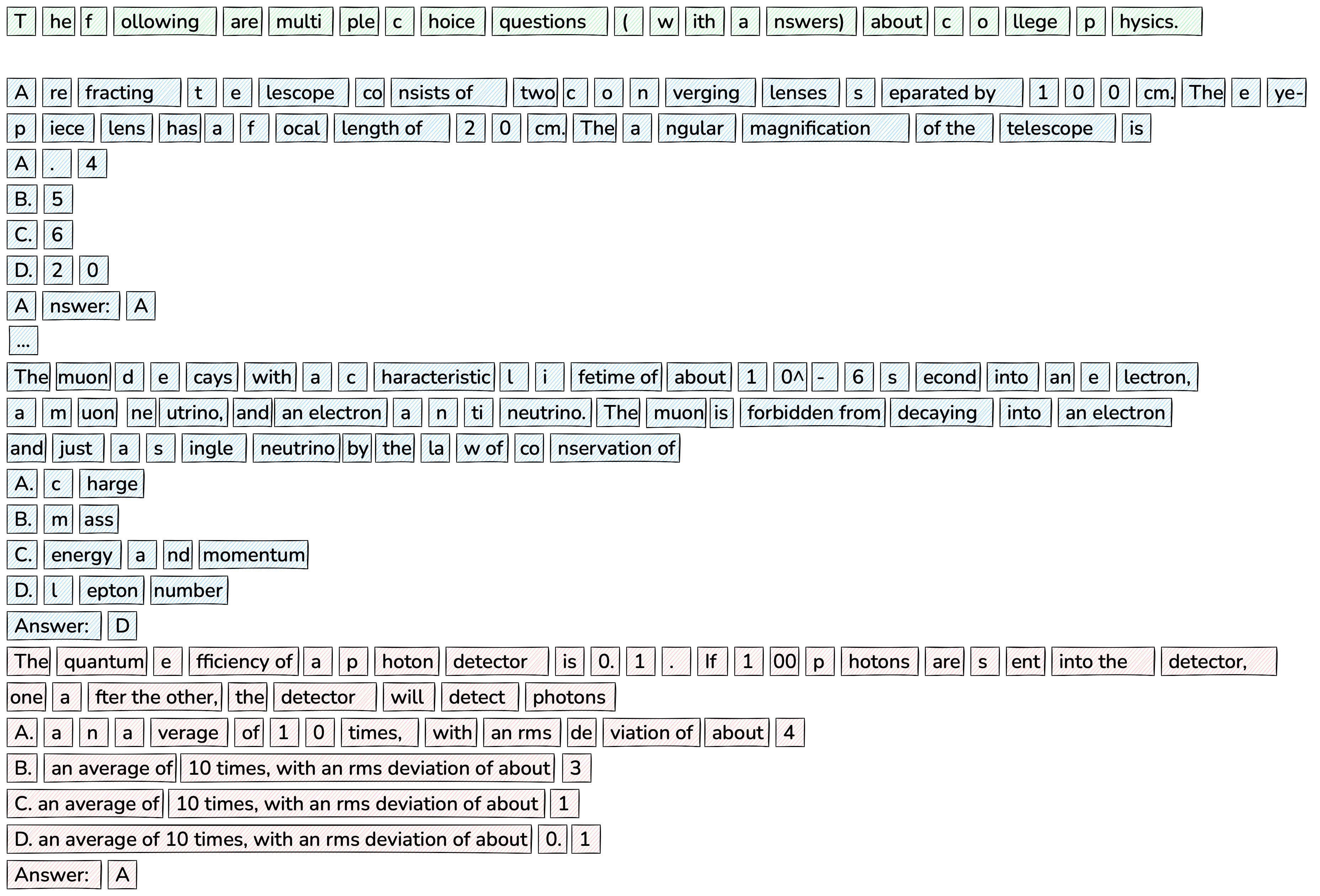
4.4 Entropy Model Context
Empirically, we find that using entropy patching yields progressively larger patches in structured content like multiple choice tasks (see patching on an MMLU example in Figure 9) which are often very repetitive. These variations are caused by lower entropy on the repeated content found in the entropy model context. So for the large scale run of BLT\text{B{\scriptsize LT}}BLT-Entropy with patch size 4.5, we reset the entropy context with new lines and use approximate monontonicity constraint as it suffers less from "entropy drift" from changes in context length. This change only affects how we compute entropies, but we still follow the same procedure to identify the value of the entropy threshold.
4.5 FLOPs Estimation
We largely follow the equations for computation of transformer fLOP\text{f{\scriptsize LOP}}fLOP s from Chinchilla ([20]) comprising fLOP\text{f{\scriptsize LOP}}fLOP s for the feed-forward layers, qKVO\text{q{\scriptsize KVO}}qKVO projections in the self-attention layer, and computation of attention and output projection. A notable difference is that we assume the input embedding layer is implemented as an efficient lookup instead of a dense matrix multiplication, therefore becoming a 0- fLOP\text{f{\scriptsize LOP}}fLOP operation. Following previous work, we estimate that the backwards pass has twice the number of fLOP\text{f{\scriptsize LOP}}fLOP s as the forward pass.
To compute fLOP\text{f{\scriptsize LOP}}fLOP s per byte for BLT\text{B{\scriptsize LT}}BLT models, we add up the fLOP\text{f{\scriptsize LOP}}fLOP s for the local encoder transformer, the global latent transformer, and the local decoder transformer, together with the cross attention blocks in the encoder and the decoder:
where nctxn_{ctx}nctx is the sequence length in bytes, npn_pnp is the patch size, rrr is the ratio of queries to key/values, kkk is the ratio of patch-dimension to byte-dimension i.e. the number of local model splits that concatenate to form a global model representation (k=2k=2k=2 in Figure 5). VVV corresponds to the vocabulary size for the output projection, which is only used in the local decoder. Depending on whether a module is applied on the byte or patch sequence, the attention uses a different context length, mmm. We modify the attention fLOP\text{f{\scriptsize LOP}}fLOP s accordingly for each component. The exact equations for fLOP\text{f{\scriptsize LOP}}fLOP s computation for Transformer-FLOPs and Cross-Attention FLOPs are provided in Appendix B.
4.6 Bits-Per-Byte Estimation
Perplexity only makes sense in the context of a fixed tokenizer as it is a measure of the uncertainty for each token. When comparing byte and token-level models, following previous work ([6, 10, 9]), we instead report Bits-Per-Byte (BPB), a tokenizer independent version of perplexity. Specifically:
where the uncertainty over the data x\pmb{x}x as measured by the sum of the cross-entropy loss is normalized by the total number of bytes in x\pmb{x}x and a constant.
4.7 Transformer Architecture Hyperparameters
For all the transformer blocks in BLT\text{B{\scriptsize LT}}BLT, i.e. both local and global models, we largely follow the architecture of Llama 3 ([11]); we use the SwiGLU activation function ([21]) in the feed-forward layers, rotary positional embeddings (RoPE) ([22]) with θ=500000\theta=500000θ=500000 ([23]) only in self-attention layers, and RMSNorm ([24]) for layer normalization. We use Flash attention ([25]) for all self-attention layers that use fixed-standard attention masks such as block causal or fixed-window block causal, and a window size of 512 for fixed-width attention masks. Since our cross-attention layers involve dynamic patch-dependent masks, we use Flex Attention to produce fused implementations and significantly speed up training.
4.8 BLT\text{B{\scriptsize LT}}BLT-Specific Hyperparameters
To study the effectiveness of BLT\text{B{\scriptsize LT}}BLT models, we conduct experiments along two directions, scaling trends, and downstream task evaluations, and we consider models at different scales: 400M, 1B, 2B, 4B and 8B for these experiments. The architecture hyperparameters for these models are presented in Appendix Table 10. We use max-pooling to initialize the queries for the first cross-attention layer in the local encoder. We use 500,000500, 000500,000 hashes with a single hash function, with n-gram sizes ranging from 3 to 8, for all BLT\text{B{\scriptsize LT}}BLT models. We use a learning rate of 4e−44e-44e−4 for all models. The choice of matching learning rate between token and BLT\text{B{\scriptsize LT}}BLT models follows a hyperparameter search between 1e−31e-31e−3 and 1e−41e-41e−4 at 400M and 1B model scales showing the same learning rate is optimal. For scaling trends on Llama-2 data, we use training batch-sizes as recommended by [11] or its equivalent in bytes. For optimization, we use the AdamW optimizer ([26]) with β1\beta_1β1 set to 0.9 and β2\beta_2β2 to 0.95, with an ϵ=10−8\epsilon=10^{-8}ϵ=10−8. We use a linear warm-up of 2000 steps with an cosine decay schedule of the learning rate to 0, we apply a weight decay of 0.1, and global gradient clipping at a threshold of 1.0.
5. Scaling Trends
In this section, the authors investigate whether byte-level models can match the scaling properties of token-based models across different training regimes. They train compute-optimal BLT models from 1B to 8B parameters on the Llama 2 dataset and demonstrate that BLT achieves parity with state-of-the-art BPE tokenizer models like Llama 3, marking the first byte-level transformer architecture to do so at compute-optimal scales. Architectural improvements including cross-attention modules and dynamic entropy-based patching prove essential for this performance. Beyond compute-optimal training, an 8B BLT model trained on the higher-quality BLT-1T dataset outperforms Llama 3 on most downstream tasks despite equivalent training budgets. A fixed-inference scaling study reveals that BLT models with larger patches consistently surpass BPE models after modest additional training beyond compute-optimal points, with this crossover occurring earlier at larger model scales. These trends indicate that simultaneously increasing patch size and model capacity enables better scaling efficiency than fixed-vocabulary tokenization.
We present a holistic picture of the scaling trends of byte-level models that can inform further scaling of BLT\text{B{\scriptsize LT}}BLT models. Our scaling study aims to address the limitations of previous research on byte-level models in the following ways: (a) We compare trends for the compute-optimal training regime, (b) We train matching 8B models on non-trivial amounts of training data (up to 1T tokens/4T bytes) and evaluate on downstream tasks, and (c) We measure scaling trends in inference-cost controlled settings. In a later section, we will investigate specific advantages from modeling byte-sequences.
5.1 Parameter Matched Compute Optimal Scaling Trends
Using the Llama 2 dataset, we train various compute-optimal bPE\text{b{\scriptsize PE}}bPE and BLT\text{B{\scriptsize LT}}BLT models across four different sizes, ranging from 1B to 8B parameters. We then plot the training fLOP\text{f{\scriptsize LOP}}fLOP s against language modeling performance on a representative subset of the training data mixture. The bPE\text{b{\scriptsize PE}}bPE models are trained using the optimal ratio of model parameters to training data, as determined by Llama 3 ([11]). This compute-optimal setup is theoretically designed to achieve the best performance on the training dataset within a given training budget ([20]), providing a robust baseline for our model. For each bPE\text{b{\scriptsize PE}}bPE model, we also train a corresponding BLT\text{B{\scriptsize LT}}BLT model on the same data, using a Latent Transformer that matches the size and architecture of the corresponding bPE\text{b{\scriptsize PE}}bPE Transformer.
As illustrated in Figure 6 (right), BLT\text{B{\scriptsize LT}}BLT models either match or outperform their bPE\text{b{\scriptsize PE}}bPE counterparts and this trend holds as we scale model size and fLOP\text{f{\scriptsize LOP}}fLOP s. To the best of our knowledge, BLT\text{B{\scriptsize LT}}BLT is the first byte-level Transformer architecture to achieve matching scaling trends with BPE-based models at compute optimal regimes. This therefore validates our assumption that the optimal ratio of parameters to training compute for bPE\text{b{\scriptsize PE}}bPE also applies to BLT\text{B{\scriptsize LT}}BLT, or at least it is not too far off.
Both architectural improvements and dynamic patching are crucial to match bPE\text{b{\scriptsize PE}}bPE scaling trends. In Figure 6 (left), we compare space-patching-based models against Llama 3. We approximate SpaceByte ([12]) using BLT\text{B{\scriptsize LT}}BLT space-patching without n-gram embeddings and cross-attention. Although SpaceByte improves over Megabyte, it remains far from Llama 3. In Figure 6 (right), we illustrate the improvements from both architectural changes and dynamic patching. BLT\text{B{\scriptsize LT}}BLT models perform on par with state-of-the-art tokenizer-based models such as Llama 3, at scale.
We also observe the effects of the choice of tokenizer on performance for tokenizer-based models, i.e., models trained with the Llama-3 tokenizer outperform those trained using the Llama-2 tokenizer on the same training data.
Finally, our BLT\text{B{\scriptsize LT}}BLT architecture trends between Llama 2 and 3 when using significantly larger patch sizes. The bPE\text{b{\scriptsize PE}}bPE tokenizers of Llama 2 and 3 have an average token size of 3.7 and 4.4 bytes. In contrast, BLT\text{B{\scriptsize LT}}BLT can achieve similar scaling trends with an average patch size of 6 and even 8 bytes. Inference fLOP\text{f{\scriptsize LOP}}fLOP are inversely proportional to the average patch size, so using a patch size of 8 bytes would lead to nearly 50% inference fLOP\text{f{\scriptsize LOP}}fLOP savings. Models with larger patch sizes also seem to perform better as we scale model and data size. BLT\text{B{\scriptsize LT}}BLT with patch size of 8 starts at a significantly worse point compared to bPE\text{b{\scriptsize PE}}bPE Llama 2 at 1B but ends up better than bPE\text{b{\scriptsize PE}}bPE at 7B scale. This suggests that such patch sizes might perform better at even larger scales and possibly that even larger ones could be feasible as model size and training compute grow.
5.2 Beyond Compute Optimal Task Evaluations
To assess scaling properties further, we train an 8B BLT\text{B{\scriptsize LT}}BLT model beyond the compute optimal ratio on the BLT\text{B{\scriptsize LT}}BLT-1T dataset, a larger higher-quality dataset, and measure performance on a suite of standard classification and generation benchmarks. For evaluation, we select the following common sense reasoning, world knowledge, and code generation tasks: Classification tasks
include ARC-Easy (0-shot) ([27]), Arc-Challenge (0-shot) ([27]), HellaSwag (0-shot) ([28]), PIQA (0-shot) ([29]), and MMLU (5-shot) ([30]). We employ a prompt-scoring method, calculating the likelihood over choice characters, and report the average accuracy. Coding related generation tasks:
We report pass@1 scores on MBPP (3-shot) ([31]) and HumanEval (0-shot) ([32]), to evaluate the ability of LLMs to generate Python code.
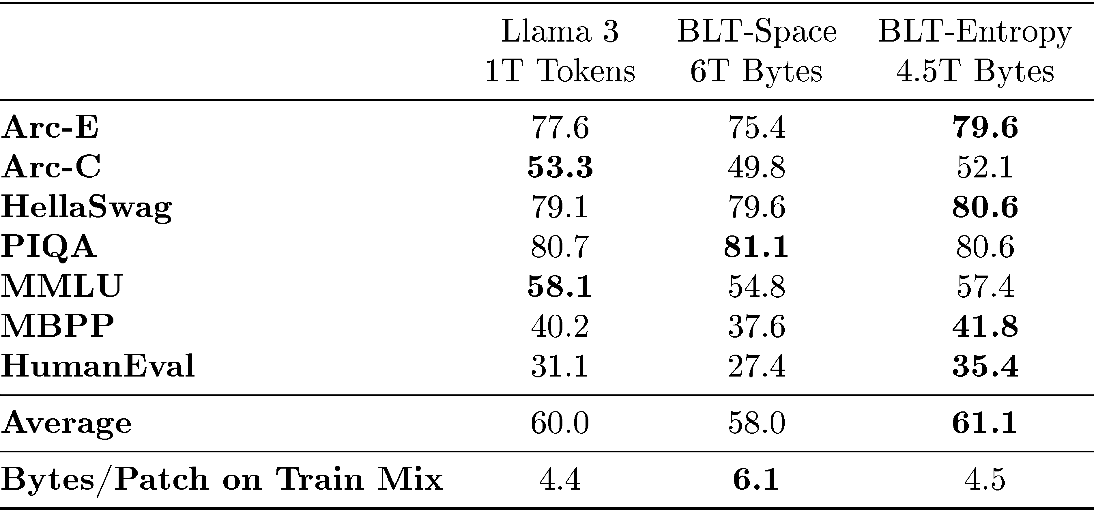
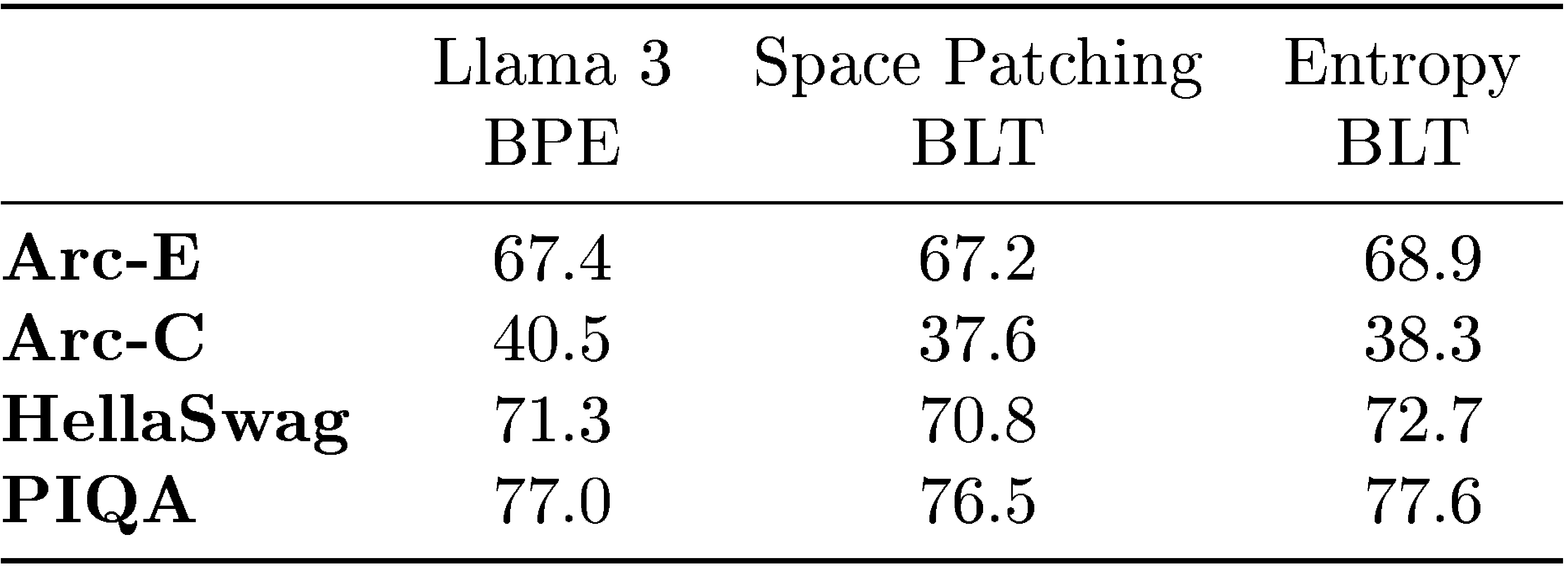
In Table 1, we compare three models trained on the BLT\text{B{\scriptsize LT}}BLT-1T dataset: a bPE\text{b{\scriptsize PE}}bPE Llama 3 tokenizer-based model, and two variants of the BLT\text{B{\scriptsize LT}}BLT model. One employing a space-patching scheme (BLT\text{B{\scriptsize LT}}BLT-Space) and another utilizing an entropy-based patching scheme (BLT\text{B{\scriptsize LT}}BLT-Entropy). with approx. monotonicity constraint and reset the context of the entropy model with new lines (as discussed in Section 4.4). All three models are trained with an equivalent fLOP\text{f{\scriptsize LOP}}fLOP budget. However, with BLT\text{B{\scriptsize LT}}BLT-Entropy we additionally make an inference time adjustment of the entropy threshold from 0.6 to 0.1 which we find to improve task performance at the cost of more inference steps.
The BLT\text{B{\scriptsize LT}}BLT-Entropy model outperforms the Llama 3 model on 4 out of 7 tasks while being trained on the same number of bytes. This improvement is like due to a combination of (1) a better use of training compute via dynamic patching, and (2) the direct modeling of byte-level information as opposed to tokens.
On the other hand, BLT\text{B{\scriptsize LT}}BLT-Space underperforms the Llama 3 tokenizer on all but one task, but it achieves a significant reduction in inference fLOP\text{f{\scriptsize LOP}}fLOP s with its larger average patch size of 6 bytes. In comparison, the bPE\text{b{\scriptsize PE}}bPE and entropy-patching based models have roughly equivalent average patch size of approximately 4.5 bytes on the training data mix. With the same training budget, the larger patch size model covers 30% more data than the other two models which might push BLT\text{B{\scriptsize LT}}BLT further away from the compute-optimal point.
:Table 2: Details of models used in the fixed-inference scaling study. We report non-embedding parameters for each model and their relative number compared to Llama 2. We pick model sizes with equal inference fLOP\text{f{\scriptsize LOP}}fLOP s per byte. We also indicate BPE's compute-optimal training data quantity and the crossover point where BLT\text{B{\scriptsize LT}}BLT surpasses BPE as seen in Figure 1 (both expressed in bytes of training data). This point is achieved at much smaller scales compared to many modern training budgets.
5.3 Patches Scale Better Than Tokens
With BLT\text{B{\scriptsize LT}}BLT models, we can simultaneously increase model size and patch size while maintaining the same training and inference fLOP\text{f{\scriptsize LOP}}fLOP budget and keeping the amount of training data constant. Arbitrarily increasing the patch size is a unique feature of patch-based models which break free of the efficiency tradeoffs of fixed-vocabulary token-based models, as discussed in Section 2.4. Longer patch sizes save compute, which can be reallocated to grow the size of the global latent transformer, because it is run less often.
We conduct a fixed inference scaling study to test the hypothesis that larger models taking fewer steps on larger patches might perform better than smaller models taking more steps. Starting from model sizes of 400m and 3.6B parameters with the Llama 2 tokenizer, we find fLOP\text{f{\scriptsize LOP}}fLOP equivalent models with the Llama 3 tokenizer and BLT\text{B{\scriptsize LT}}BLT-Entropy models with average patch sizes of 6 and 8 bytes on the training datamix (see Table 2 for model details). For patch size 8 models, we use 3 encoder layers instead of 1. We train each model for various training fLOP\text{f{\scriptsize LOP}}fLOP budgets.
Figure 1 shows that BLT\text{B{\scriptsize LT}}BLT models achieve better scaling trends than tokenization-based architectures for both inference fLOP\text{f{\scriptsize LOP}}fLOP classes. In both cases, BPE models perform better with small training budgets and are quickly surpassed by BLT\text{B{\scriptsize LT}}BLT, not far beyond the compute-optimal regime. In practice, it can be preferable to spend more during the one-time pretraining to achieve a better performing model with a fixed inference budget. A perfect example of this is the class of 8B models, like Llama 3.1, which has been trained on two orders of magnitude more data than what is compute-optimal for that model size.
The crossover point where BLT\text{B{\scriptsize LT}}BLT improves over token-based models has shifted slightly closer to the compute-optimal point when moving to the larger fLOP\text{f{\scriptsize LOP}}fLOP class models (from 3x down to 2.5x the compute optimal budget). Similarly, the larger patch size 8 model has steeper scaling trend in the larger fLOP\text{f{\scriptsize LOP}}fLOP class overtaking the other models sooner. As discussed in Section 5.1, larger patch sizes appear to perform closer to BPE models at larger model scales. We attribute this, in part, to the decreasing share of total fLOP\text{f{\scriptsize LOP}}fLOP s used by the byte-level Encoder and Decoder modules which seem to scale slower than the Latent Transformer. When growing total parameters 20x from 400M to 8B, we only roughly double BLT\text{B{\scriptsize LT}}BLT 's local model parameters. This is important as larger patch sizes only affect fLOP\text{f{\scriptsize LOP}}fLOP s from the patch Latent Transformer and not the byte-level modules. In fact, that is why the BLT\text{B{\scriptsize LT}}BLT-Entropy ps=8 went from 1.6x to 1.7x of the Llama 2 model size when moving to the larger model scale.
In summary, our patch-length scaling study demonstrates that the BLT\text{B{\scriptsize LT}}BLT patch-based architecture can achieve better scaling trends by simultaneously increasing both patch and model size. Such trends seem to persist and even improve at larger model scales.
6. Byte Modeling Improves Robustness
In this section, the authors demonstrate that BLT's byte-level modeling provides significant robustness advantages over tokenizer-based models across multiple dimensions. They evaluate BLT on character-level tasks including noisy text classification (where various character-level perturbations are applied), grapheme-to-phoneme conversion, character manipulation tasks from the CUTE benchmark, and low-resource machine translation. BLT consistently outperforms Llama 3 models trained on equivalent data, achieving an 8-point advantage on noised text, over 25 points higher on CUTE (reaching 99.9% on spelling tasks), and 2-point improvements on low-resource translation into English. These gains persist even when comparing against Llama 3.1 trained on 16x more data, suggesting that character-level awareness is difficult for BPE models to acquire through additional training alone. Additionally, the authors show that BLT can leverage existing pretrained tokenizer-based models by initializing BLT's global transformer from Llama 3.1 weights, effectively converting tokenizer-based models into tokenizer-free ones while maintaining strong performance with reduced training compute.
We also measure the robustness of BLT\text{B{\scriptsize LT}}BLT compared to token-based models that lack direct byte-level information, and present an approach to byte-ify pretrained token-based models.
6.1 Character-Level Tasks
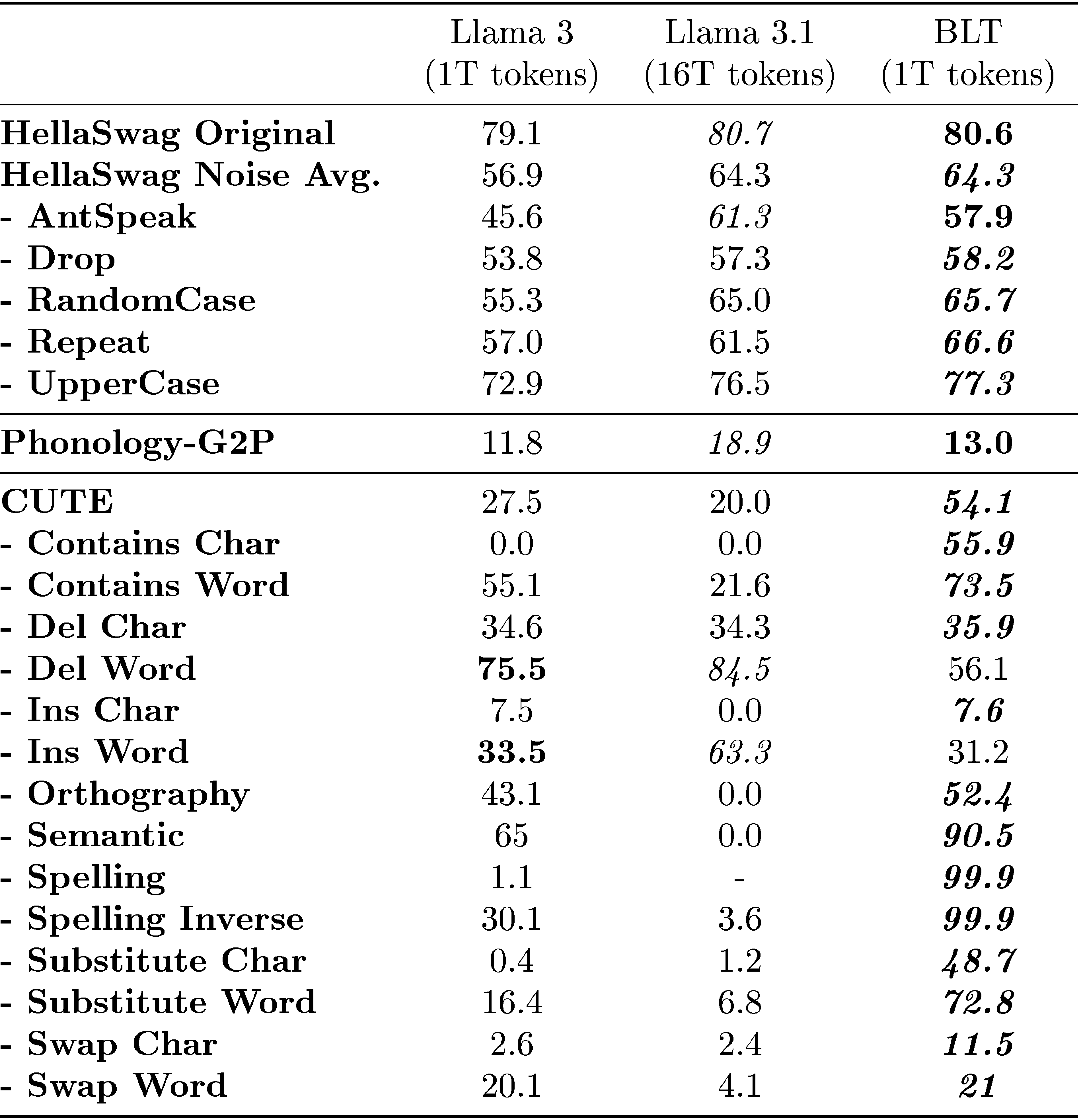
A very early motivation for training byte-level models was to take advantage of their robustness to byte level noise in the input, and also to exploit their awareness of the constituents of tokens, which current tokenizer-based models struggle with. To measure these phenomena, we perform additional evaluations on benchmarks that evaluate both robustness to input noise as well as awareness of characters, both English and multi-lingual, including digits and phonemes. We present these results in Table 3.
Noisy Data
We create noised versions of the benchmark classification tasks described in Section 5.2, to compare the robustness of tokenizer-based models with that of BLT\text{B{\scriptsize LT}}BLT. We employ five distinct character-level noising strategies to introduce variations in the text: (a) AntSpeak: This strategy converts the entire text into uppercase, space-separated characters. (b) Drop: Randomly removes 10% of the characters from the text. (c) RandomCase: Converts 50% of the characters to uppercase and 50% to lowercase randomly throughout the text. (d) Repeat: Repeats 20% of the characters up to a maximum of four times. (e) UpperCase: Transforms all characters in the text to uppercase. During evaluation, we apply each noising strategy to either the prompt, completion, or both as separate tasks and report the average scores. In Table 3 we report results on noised HellaSwag ([28]) and find that BLT\text{B{\scriptsize LT}}BLT indeed outperforms tokenizer-based models across the board in terms of robustness, with an average advantage of 8 points over the model trained on the same data, and even improves over the Llama 3.1 model trained on a much larger dataset.
Phonology - Grapheme-to-Phoneme (G2P)
We assess BLT\text{B{\scriptsize LT}}BLT 's capability to map a sequence of graphemes (characters representing a word) into a transcription of that word's pronunciation (phonemes). In Table 3, we present the results of the G2P task in a 5-shot setting using Phonology Bench ([34]) and find that BLT\text{B{\scriptsize LT}}BLT outperforms the baseline Llama 3 1T tokenizer-based model on this task.
CUTE
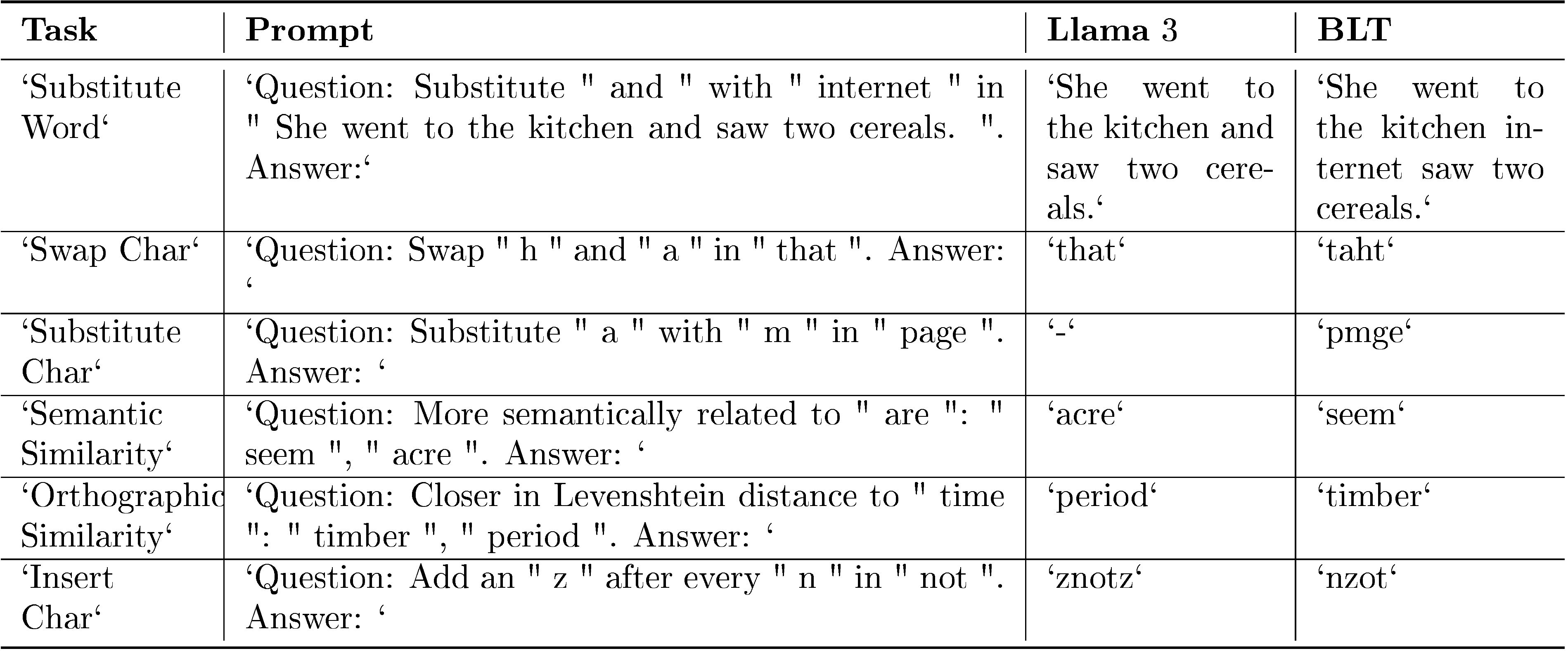
To assess character-level understanding, we evaluate BLT\text{B{\scriptsize LT}}BLT on the CUTE benchmark ([2]), which comprises several tasks that are broadly classified into three categories: understanding composition, understanding orthographic similarity, and ability to manipulate sequences. This benchmark poses a significant challenge for most tokenizer-based models, as they appear to possess knowledge of their tokens' spellings but struggle to effectively utilize this information to manipulate text. Table 3 shows that BLT\text{B{\scriptsize LT}}BLT-Entropy outperforms both BPE Llama 3 models by more than 25 points on this benchmark. In particular, our model demonstrates exceptional proficiency in character manipulation tasks achieving 99.9% on both spelling tasks. Such large improvements despite BLT\text{B{\scriptsize LT}}BLT having been trained on 16x less data than Llama 3.1 indicates that character level information is hard to learn for BPE models. Figure 7 illustrates a few such scenarios where Llama 3 tokenizer model struggles but our BLT\text{B{\scriptsize LT}}BLT model performs well. Word deletion and insertion are the only two tasks where BPE performs better. Such word manipulation might not be straightforward for a byte-level model but the gap is not too wide and building from characters to words could be easier than the other way around. We use the same evaluation setup in all tasks and the original prompts from Huggingface. BPE models might benefit from additional prompt engineering.
Low Resource Machine Translation
We evaluate BLT\text{B{\scriptsize LT}}BLT on translating into and out of six popular language families and twenty one lower resource languages with various scripts from the FLORES-101 benchmark ([33]) and report SentencePiece BLEU in Table 4. Our results demonstrate that BLT\text{B{\scriptsize LT}}BLT outperforms a model trained with the Llama 3 tokenizer, achieving a 2-point overall advantage in translating into English and a 0.5-point advantage in translating from English. In popular language pairs, BLT\text{B{\scriptsize LT}}BLT performs comparably to or slightly better than Llama 3. However, BLT\text{B{\scriptsize LT}}BLT outperforms Llama 3 on numerous language pairs within lower-resource language families, underscoring the effectiveness of byte modeling for generalizing to long-tail byte sequences.
6.2 Training BLT\text{B{\scriptsize LT}}BLT from Llama 3
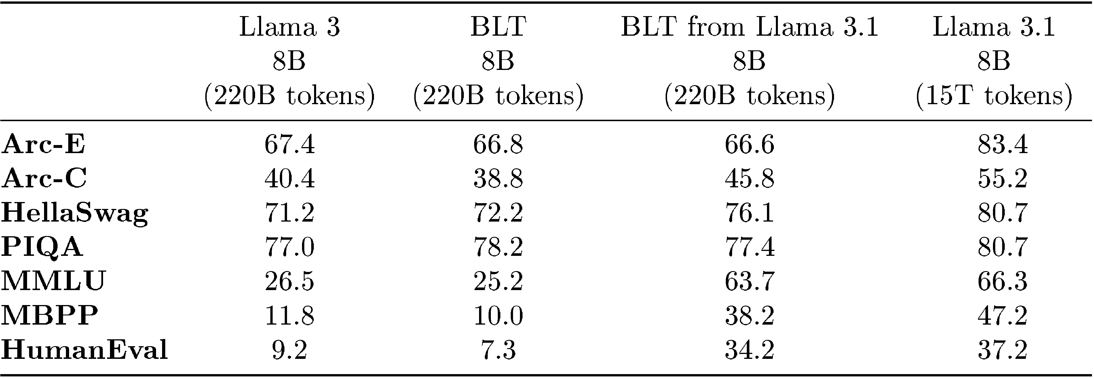
We explore a workflow where BLT\text{B{\scriptsize LT}}BLT models can leverage existing pre-trained tokenizer-based models for better and faster training convergence, acheived by initializing the global transformer parameters of BLT\text{B{\scriptsize LT}}BLT with those of a pre-trained Llama 3.1 model. Subsequently, we update the weights of the global transformer using one-tenth the learning rate employed for the local encoder and local decoder model, for Llama 3 optimal number of steps, and present a comparison with a baseline BLT\text{B{\scriptsize LT}}BLT in Table 5. It is evident that BLT\text{B{\scriptsize LT}}BLT from Llama 3.1 significantly outperforms both the Llama 3 and BLT\text{B{\scriptsize LT}}BLT baselines, which were trained with the same number of fLOP\text{f{\scriptsize LOP}}fLOP s. Moreover, when compared to our BLT\text{B{\scriptsize LT}}BLT-Entropy model (as presented in Table 1), which was trained on a significantly larger dataset (1T tokens), BLT\text{B{\scriptsize LT}}BLT from Llama 3.1 still achieves superior performance on MMLU task, suggesting that it can be an effective approach in significantly reducing the training fLOP\text{f{\scriptsize LOP}}fLOP s.
This setup can also be viewed as transforming tokenizer-based models into tokenizer-free ones, effectively converting a pre-trained LLaMA 3.1 model into a BLT\text{B{\scriptsize LT}}BLT model. To provide a comprehensive comparison, we include the original LLaMA 3.1 model trained on 15T tokens in Table 5 and evaluate it against the BLT\text{B{\scriptsize LT}}BLT derived from LLaMA 3. Our model experiences a slight performance decline on MMLU and HumanEval, but a more significant drop on other tasks. This suggests that further work is needed to fully leverage the pre-trained model and improve upon its performance, particularly in terms of optimizing data mixtures and other hyperparameters.
7. Ablations and Discussion
In this section, the authors justify architectural choices for BLT through systematic ablations on entropy model hyperparameters, patching schemes, and local model design. They find that entropy model performance improves with both larger model size and longer context windows, with diminishing returns beyond 50 million parameters and 512-byte contexts. Comparing patching approaches, dynamic entropy-based patching outperforms static methods and matches or exceeds BPE tokenization on downstream benchmarks, while space-based patching proves a competitive simpler alternative. Cross-attention in the decoder provides the most significant benefit, particularly for larger patches and Common Crawl data, with encoder cross-attention showing modest gains only when using pooled initialization. Hash n-gram embeddings dramatically improve performance across all domains, especially Wikipedia and Github, with gains plateauing around 300,000 vocabulary size and proving complementary to cross-attention benefits. Finally, when combined with hash embeddings, BLT requires only a single-layer lightweight encoder, allowing computational resources to be reallocated toward a heavier decoder for optimal performance.
In this section, we discuss ablations justifying architectural choices for BLT\text{B{\scriptsize LT}}BLT and the patching scheme and hyper-parameters for the BLT\text{B{\scriptsize LT}}BLT 8B parameter model trained on the BLT\text{B{\scriptsize LT}}BLT-1T dataset.
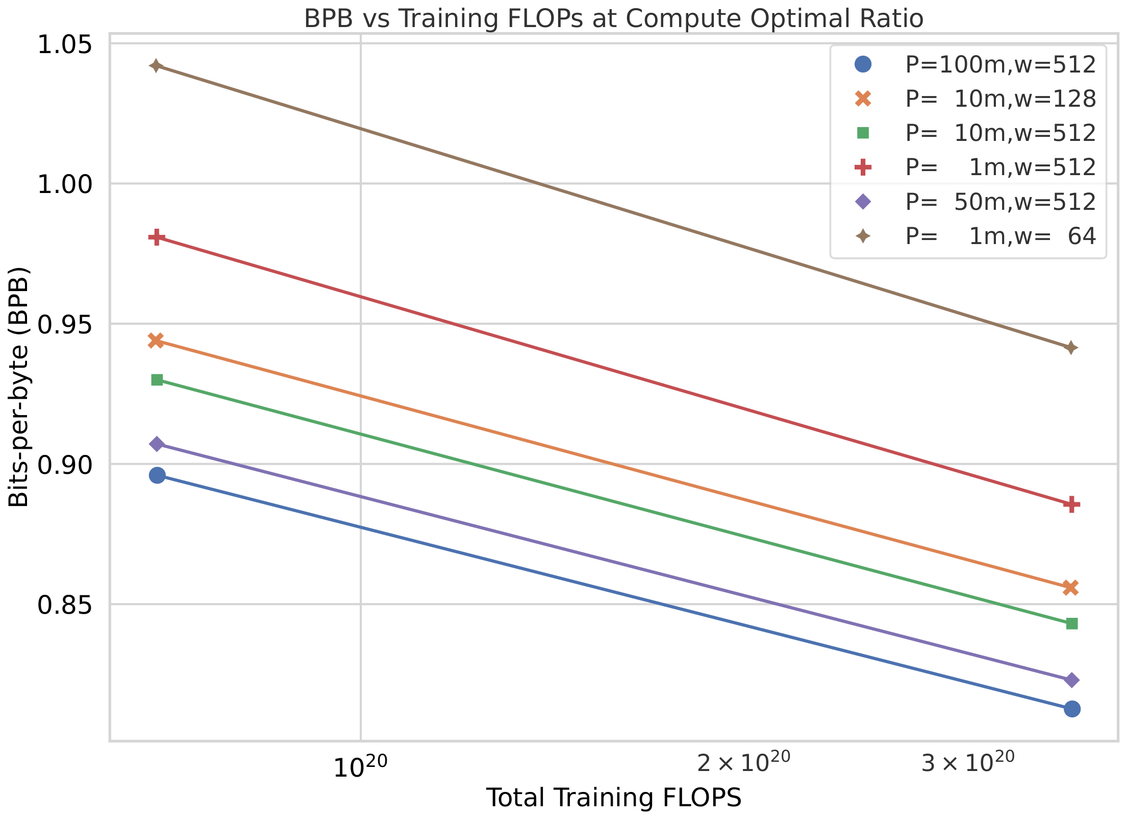
Entropy Model Hyper-parameters
To study the effect of varying entropy model size and context window length on scaling performance, we train byte-level entropy transformer models of different model sizes between 1m and 100m parameters, with varying context window lengths from 64 to 512. We plot bpb vs training fLOP\text{f{\scriptsize LOP}}fLOP scaling law curves, created using our 400m400m400m and 1b1b1b BLT\text{B{\scriptsize LT}}BLT models trained on the Llama-2 dataset and present them in Figure 8. We find that scaling performance is positively correlated with both these dimensions of the entropy model, with diminishing returns when we scale beyond 50m parameters.
Types of Patching
We ablate the four different patching schemes, introduced in Section 2 i.e. 1) Strided Patching with a stride of 4 and 6, 2) Patching on whitepsace, 3) BPE Tokenizer patching based on the Llama 3 tokenizer, and 4) Entropy based patching using a small byte lLM\text{l{\scriptsize LM}}lLM.
While dynamic patching reduces the effective length of sequences, we control for the sequence length to maintain a similar context length for all patching schemes. All the models see the same number of bytes in each sequence during training and inference in expectation to prevent any confounding factors from being able to model larger contexts. Figure 6 highlights the results of these ablations. All the remaining patching schemes outperform static patching, with space patching being a very close competitor to dynamic entropy based patching.
In Table 6, we present benchmark evaluations for BLT\text{B{\scriptsize LT}}BLT models comparing tokenizer-based models, space patching, and entropy-based patching, trained on the Llama 2 dataset for an optimal number of steps ([11]). Although space patching is a simpler strategy that does not involve running an entropy model on the fly during training, we find that the gains we observed using entropy-based patching on scaling trends (Section 5) do indeed carry forward even to downstream benchmark tasks.
Cross-Attention
In Table 7, we ablate including cross-attention at various points in the encoder and decoder of BLT\text{B{\scriptsize LT}}BLT. For the encoder cross-attention we test initializing the queries with 1) the same learned embedding for every global state, 2) a hash embedding of the bytes in the patch, and 3) pooling of the encoder hidden representation of the patch bytes at the given encoder layer.
We find that using cross-attention in the decoder is most effective. In the encoder, there is a slight improvement in using cross-attention but only with pooling initialization of queries. Additionally, we find that cross-attention helps particularly on Common-Crawl and especially with larger patch sizes.
n-gram Hash Embeddings
We ablate settings of 0, 100K, 200K and 400K n-gram hash embedding vocabularies and present results in Table 8. We find that hash embeddings help on all domains, but particularly on Wikipedia and Github (0.04 bpb difference compared to 0.01 bpb difference after 15k steps at 8B). At 8B scale going from 500K to 300K hashes changed performance by 0.001 bpb on 15k steps. This indicates that hashes are vital to bringing the performance of BLT\text{B{\scriptsize LT}}BLT to match those of tokenizer based models, however, after 300K hashes, there are diminishing returns. Additionally, it appears that the gains are largely complementary with cross-attention as they provide improvements on different datasets.
Local Model Hyperparamaters
In Table 9, we ablate various settings for the number of layers in the local encoder and decoder. When paired with hash n-gram embeddings, BLT\text{B{\scriptsize LT}}BLT works well with an encoder that is extremely light-weight i.e. just one layer, and with a heavier decoder.
8. Related Work
In this section, the evolution of character-level and byte-level language modeling is traced from early RNN-based approaches through modern transformer architectures, culminating in the development of BLT. Character-level RNNs demonstrated early promise in handling out-of-vocabulary words and morphologically rich languages but struggled to match word-level model performance. The introduction of transformers with subword tokenization improved results but imposed implicit inductive biases. While some byte-level transformers showed competitive performance, they required substantially more compute due to longer sequences. Patching-based approaches emerged to address this inefficiency, with methods like MegaByte using static patches and achieving parity with tokenizer-based models at 1B parameters on 400B bytes. However, static patching still lags behind state-of-the-art compute-optimal tokenizer models, motivating BLT's dynamic entropy-based patching strategy to bridge this performance gap while maintaining byte-level modeling benefits.
Character-Level RNNs: Character Language Modeling has been a popular task ever since the early days of neural models ([35, 36, 37]) owing to their flexibility of modeling out of vocabulary words organically without resorting to back-off methods. [38] also train a model that processes characters only on the input side using convolutional and highway networks that feed into LSTM-based RNNs and are able to match performance with the RNN based state-of-the-art language models of the time on English and outperform them on morphologically rich languages, another sought-after advantage of character-level LLMs. [39] do machine comprehension using byte-level LSTM models that outperformed word-level models again on morphologically-rich Turkish and Russian languages. Along similar lines, [40] used character-based convolutional models for classification tasks, which outperformed word-level models for certain tasks. [41] use hierarchical LSTM models using boundary-detectors at each level to discover the latent hierarchy in text, to further improve performance on character level language modeling. ByteNet by [42] uses CNN based layers on characters as opposed to attention for machine translation.
Character-Level Transformers: The development of transformer models using attention ([43]) together with subword tokenization ([15]), significantly improved the performance of neural models on language modeling and benchmark tasks. However, word and sub-word units implicitly define an inductive bias for the level of abstraction models should operate on. To combine the successes of transformer models with the initial promising results on character language modeling, [44] use very deep transformers, and with the help of auxiliary losses, train transformer-based models that outperformed previous LSTM based character lLM\text{l{\scriptsize LM}}lLM s. However, they still saw a significant gap from word level LLMs. GPT-2 ([45]) also observed that on large scale datasets like the 1 billion word benchmark, byte-level LMs were not competitive with word-level LMs.
While [46] demonstrated that byte-level lLM\text{l{\scriptsize LM}}lLM s based on transformers can outperform subword level LLMs with comparable parameters, the models take up much more compute and take much longer to train. Similarly, [7] train a BERT model (CharFormer) that builds word representations by applying convolutions on character embeddings, and demonstrate improvements on the medical domain, but they also expend much more compute in doing so. [8] develop CANINE, a 150M parameter encoder-only model that operates directly on character sequences. CANINE uses a deep transformer stack at its core similar in spirit to our global model, and a combination of a local transformer and strided convolutions to downsample the input characters, and outperforms the equivalent token-level encoder-only model (mBERT) on downstream multilingual tasks. ByT5 ([6]) explored approaches for byte-level encoder decoder models, that do not use any kind of patching operations. While their model exhibited improved robustness to noise, and was competitive with tokenizer-based models with 4x less data, the lack of patching meant that the models needed to compute expensive attention operations over every byte, which was extremely compute heavy. Directly modeling bytes instead of subword units increases the sequence length of the input making it challenging to efficiently scale byte level models. Recently, using the Mamba Architecture ([47]), which can maintain a fixed-size memory state over a very large context length, [9] train a byte-level Mamba architecture also without using patching, and are able to outperform byte-level transformer models in a fLOP\text{f{\scriptsize LOP}}fLOP controlled setting at the 350M parameter scale in terms of bits-per-byte on several datasets.
Patching-based approaches: The effective use of patching can bring down the otherwise inflated number of fLOP\text{f{\scriptsize LOP}}fLOP s expended by byte-level LLMs while potentially retaining performance, and many works demonstrated initial successes at a small scale of model size and number of training bytes. [48] experiment with static patching based downsampling and upsampling and develop the hourglass transformer which outperforms other byte-level baselines at the 150M scale. [13] further improve this with the help of dynamic patching schemes, including a boundary-predictor that is learned in an end-to-end fashion, a boundary-predictor supervised using certain tokenizers, as well as an entropy-based patching model similar to BLT\text{B{\scriptsize LT}}BLT, and show that this approach can outperform the vanilla transformers of the time on language modeling tasks at a 40M parameter scale on 400M tokens. [49] investigate training on sequences compressed using arithmetic coding to achieve compression rates beyond what BPE can achieve, and by using a equal-info windows technique, are able to outperform byte-level baselines on language modeling tasks, but underperform subword baselines.
Our work draws inspiration and is most closely related to MegaByte ([10]), which is a decoder only causal LLM that uses a fixed static patching and concatenation of representations to convert bytes to patches, and uses a local model on the decoder side to convert from patches back into bytes. They demonstrate that MegaByte can match tokenizer-based models at a 1B parameter scale on a dataset of 400B bytes. We ablate MegaByte in all our experiments and find that static patching lags behind the current state-of-the-art compute optimally trained tokenizer based models in a fLOP\text{f{\scriptsize LOP}}fLOP controlled setting and we demonstrate how BLT\text{B{\scriptsize LT}}BLT bridges this gap. [12] make the same observation about MegaByte and suggest extending the static patching method to patching on whitespaces and other space-like bytes, and also add a local encoder model. They find improvements over tokenized-based transformer models in a compute controlled setting on some domains such as Github and arXiv at the 1B parameter scale. We also report experiments with this model, and show that further architectural improvements are needed to scale up byte-level models even further and truly match current state-of-the-art token-based models such as Llama 3.
9. Limitations and Future Work
In this section, the authors identify three main areas where BLT requires further development and exploration. First, they acknowledge that their models were trained using scaling laws optimized for BPE-based transformers, which may not yield optimal parameter-to-data ratios for BLT, suggesting that calculating BLT-specific scaling laws could reveal even better performance trends. Second, while their experiments present theoretically FLOP-matched comparisons using efficient implementations like FlexAttention, the current BLT codebase has not achieved wall-clock parity with highly optimized tokenizer-based transformer libraries, indicating room for implementation improvements. Third, BLT currently relies on a separately trained entropy model for dynamic patching, and learning this patching mechanism end-to-end could enhance performance. Additionally, preliminary experiments suggest that "byte-ifying" pretrained models like Llama 3 by freezing their weights as the global transformer shows promise, potentially enabling models to surpass tokenizer-based performance without requiring full retraining from scratch.
In this work, for the purposes of architectural choices, we train models for the optimal number of steps as determined for Llama 3 ([11]). However, these scaling laws were calculated for BPE-level transformers and may lead to suboptimal (data, parameter sizes) ratios in the case of BLT\text{B{\scriptsize LT}}BLT. We leave for future work the calculation of scaling laws for BLT\text{B{\scriptsize LT}}BLT potentially leading to even more favorable scaling trends for our architecture. Additionally, many of these experiments were conducted at scales upto 1B parameters, and it is possible for the optimal architectural choices to change as we scale to 8B parameters and beyond, which may unlock improved performance for larger scales.
Existing transformer libraries and codebases are designed to be highly efficient for tokenizer-based transformer architectures. While we present theoretical fLOP\text{f{\scriptsize LOP}}fLOP matched experiments and also use certain efficient implementations (such as FlexAttention) to handle layers that deviate from the vanilla transformer architecture, our implementations may yet not be at parity with tokenizer-based models in terms of wall-clock time and may benefit from further optimizations.
While BLT\text{B{\scriptsize LT}}BLT uses a separately trained entropy model for patching, learning the patching model in an end-to-end fashion can be an interesting direction for future work. In Section 6.2, we present initial experiments showing indications of success for "byte-ifying" tokenizer-based models such as Llama 3 that are trained on more than 10T tokens, by initializing and freezing the global transformer with their weights. Further work in this direction may uncover methods that not only retain the benefits of bytefying, but also push performance beyond that of these tokenizer-based models without training them from scratch.
10. Conclusion
In this section, the authors establish that the Byte Latent Transformer (BLT) fundamentally reimagines language modeling by eliminating fixed-vocabulary tokenization in favor of dynamic, learnable byte grouping into patches. This architecture allocates computational resources adaptively based on data complexity, yielding substantial gains in efficiency and robustness. Extensive scaling experiments demonstrate that BLT matches tokenization-based models like Llama 3 at scales reaching 8B parameters and 4T bytes, while enabling up to 50% inference FLOP reductions with minimal performance trade-offs. Critically, BLT introduces a novel scaling dimension where model and patch sizes can grow simultaneously within fixed inference budgets, proving advantageous in practical compute regimes. By processing raw bytes directly, BLT exhibits superior robustness to noisy inputs and deeper sub-word understanding, positioning it as a compelling alternative to traditional tokenization approaches for building scalable, adaptable language models.
This paper presents the Byte Latent Transformer (BLT), a new architecture that redefines the conventional dependency on fixed-vocabulary tokenization in large language models. By introducing a dynamic, learnable method for grouping bytes into patches, BLT\text{B{\scriptsize LT}}BLT effectively allocates computational resources based on data complexity, leading to significant improvements in both efficiency and robustness. Our extensive scaling study demonstrates that BLT\text{B{\scriptsize LT}}BLT models can match the performance of tokenization-based models like Llama 3 at scales up to 8B and 4T bytes, and can trade minor losses in evaluation metrics for up to 50% reductions in inference fLOP\text{f{\scriptsize LOP}}fLOP s. Furthermore, BLT\text{B{\scriptsize LT}}BLT unlocks a new dimension for scaling, allowing simultaneous increases in model and patch size within a fixed inference budget. This new paradigm becomes advantageous for compute regimes commonly encountered in practical settings. While directly engaging with raw byte data, BLT\text{B{\scriptsize LT}}BLT also improves the model's ability to handle the long-tail of data, offering significant improvements in robustness to noisy inputs and a deeper understanding of sub-word structures. Overall, these results position BLT\text{B{\scriptsize LT}}BLT as a promising alternative to traditional tokenization-based approaches, providing a scalable and robust framework for more efficient and adaptable language models.
Acknowledgements
In this section, the authors acknowledge the extensive collaborative support that enabled the development and evaluation of BLT. Kalyan Saladi provided critical pre-training infrastructure assistance, while Gabriel Synnaeve, Ammar Rizvi, Jacob Kahn, and Michel Meyer helped organize computational resources necessary for scaling experiments. Badr Youbi Idirissi, Mathurin Videau, and Jade Copet contributed through technical discussions, provided access to the Lingua framework for open-sourcing BLT's code, and assisted in preparing the BLT-1T dataset that underpinned the research. Omer Levy's early-stage involvement shaped the project's direction through valuable feedback and ideas. Driss Guessous supported the implementation of FlexAttention, a key optimization technique. Finally, Sida Wang, Melanie Sclar, Amanda Bertsch, and Hunter Lang offered ongoing feedback and engaged in discussions that refined the work. These contributions collectively enabled the successful development, scaling, and evaluation of the Byte Latent Transformer architecture.
We would like to thank Kalyan Saladi for help with everything relating to pre-training infrastructure; Gabriel Synnaeve, Ammar Rizvi, Jacob Kahn, Michel Meyer for helping organize resources for scaling up BLT\text{B{\scriptsize LT}}BLT; Badr Youbi Idirissi, Mathurin Videau, and Jade Copet for invaluable discussions and feedback about BLT\text{B{\scriptsize LT}}BLT, for access to the Lingua framework for open-sourcing code for BLT\text{B{\scriptsize LT}}BLT, and for help preparing the BLT\text{B{\scriptsize LT}}BLT-1T dataset used in this paper; Omer Levy, who was actively involved in the early stages of the project and provided valuable feedback and ideas; Driss Guessous for help with FlexAttention; and Sida Wang, Melanie Sclar, Amanda Bertsch, and Hunter Lang for feedback and discussions.
11. Contributors
In this section, the contributors to the Byte Latent Transformer (BLT) research project are organized into three tiers based on their level of involvement. The core contributors who drove the primary research and development include Artidoro Pagnoni, Srinivasan Iyer, Ramakanth Pasunuru, Pedro Rodriguez, John Nguyen, and Gargi Ghosh, who served as the project lead. The core advising group, comprising Mike Lewis, Ari Holtzman, and Luke Zettlemoyer, provided strategic guidance and expertise throughout the project's development. Additional advisors and contributors, including Jason Weston, Benjamin Muller, Margaret Li, Chunting Zhou, and Lili Yu, offered specialized knowledge and support in various aspects of the research. This collaborative structure reflects a hierarchical approach to managing a complex machine learning research effort, ensuring clear delineation of responsibilities while leveraging diverse expertise across the team.
In this section, we list individual contributions.
Core Contributors:
Artidoro Pagnoni, Srinivasan Iyer, Ramakanth Pasunuru, Pedro Rodriguez, John Nguyen, Gargi Ghosh (Project Lead)
Core Advising Group:
Mike Lewis, Ari Holtzman, Luke Zettlemoyer
Advisors and Contributors:
Jason Weston, Benjamin Muller, Margaret Li, Chunting Zhou, Lili Yu
Appendix
A. Model Hyper Parameters
Table 10 shows different hyper parameter settings for BLT\text{B{\scriptsize LT}}BLT models.
B. FLOPs Equations
Here, we provide the equations used for fLOP\text{f{\scriptsize LOP}}fLOP computation for the forward-pass of transformer and BLT\text{B{\scriptsize LT}}BLT models based on [20, 50, 51]. We assume that the backward pass uses twice as much fLOP\text{f{\scriptsize LOP}}fLOP s as the forward pass.
:Table 11: fLOP\text{f{\scriptsize LOP}}fLOP s for operations used in transformer and BLT\text{B{\scriptsize LT}}BLT models. lll corresponds to layers, hhh is the hidden dimension (hkh_khk with nheadsn_{heads}nheads heads), mmm is the context length, dff=4d_{ff}=4dff=4 is the feed-forward dimension multiplier, ppp is the patch size, and rrr is the ratio of queries to keys.
For a transformer model with lll layers, hidden dimension hhh, context length mmm, nheadsn_{heads}nheads attention heads of dimension hkh_khk, and a feed-forward multipler of dffd_{ff}dff, we compute fLOP\text{f{\scriptsize LOP}}fLOP s as:
For BLT\text{B{\scriptsize LT}}BLT models, we use the above-mentioned primitives together with the fLOP\text{f{\scriptsize LOP}}fLOP s equation from Section 4.5 to compute total fLOP\text{f{\scriptsize LOP}}fLOP s.
C. Rolling Polynomial Hashing
Given a byte nnn-gram gi,n={bi−n+1,…,bi}g_{i, n}=\{b_{i-n + 1}, \ldots, b_i\}gi,n={bi−n+1,…,bi}, the rolling polynomial hash of gi,ng_{i, n}gi,n is defined as:
Where aaa is chosen to be a 10-digit prime number.
D. Frequency-based n-gram Embedddings
Prior to using hash n-gram embeddings in the final BLT\text{B{\scriptsize LT}}BLT architecture, we also experimented with frequency-based n-gram embeddings. For each n∈{1,2,3,4,5,6,7,8}n\in\{1, 2, 3, 4, 5, 6, 7, 8\}n∈{1,2,3,4,5,6,7,8} there is an embedding matrix EnngramE_{n}^{ngram}Enngram that contains the most frequent byte-grams for the given nnn. Since it is intractable to store embeddings as nnn grows, we only store embeddings for the most frequent 100,000100, 000100,000 byte-grams for each byte-gram. If a particular position iii includes an nnn-gram present in the corresponding the embedding matrix, then this embedding is passed to the next step, encoder multi-headed cross-attention. If a byte-gram is infrequent and therefore not in the matrix, then its embedding is obtained from encoder hash embeddings instead.
Since frequency-based nnn-grams are limited by the vocabulary of the n-gram tables with infrequent n-grams not being represented at all, we subsequently moved to hash-based nnn-gram embeddings. See Table 12 for a comparison of hash and frequency based n-gram embeddings.
E. Entropy Patching Example from MMLU
We illustrate how a few-shot example from a downstream task i.e. MMLU ([30]), is patched using an entropy-model trained for use with BLT\text{B{\scriptsize LT}}BLT models in Figure 9. Directly using the entropy model with the full-context window causes repetitive patterns to be heavily patched. For example, "10 times, with an rms deviation of about" in the MMLU query is patched frequently the first time it is encountered, but is part of very large patches the next three times, which, although inference efficient, maybe undesirable for reasoning. One method that we use to avoid such a "entropy" drift is by resetting the entropy context with new lines and using a approximate monotonicity constraint (see Section 4.4).
References
[1] Gautier Dagan, Gabriel Synnaeve, and Baptiste Roziere. Getting the most out of your tokenizer for pre-training and domain adaptation. In Forty-first International Conference on Machine Learning, 2024.
[2] Lukas Edman, Helmut Schmid, and Alexander Fraser. CUTE: Measuring llms' understanding of their tokens. arXiv, 2024.
[3] Davis Liang, Hila Gonen, Yuning Mao, Rui Hou, Naman Goyal, Marjan Ghazvininejad, Luke Zettlemoyer, and Madian Khabsa. Xlm-v: Overcoming the vocabulary bottleneck in multilingual masked language models. In Proceedings of Empirical Methods in Natural Language Processing, 2023.
[4] Aleksandar Petrov, Emanuele La Malfa, Philip Torr, and Adel Bibi. Language model tokenizers introduce unfairness between languages. Proceedings of Advances in Neural Information Processing Systems, 2024.
[5] Tomasz Limisiewicz, Terra Blevins, Hila Gonen, Orevaoghene Ahia, and Luke Zettlemoyer. Myte: Morphology-driven byte encoding for better and fairer multilingual language modeling. arXiv, 2024.
[6] Linting Xue, Aditya Barua, Noah Constant, Rami Al-Rfou, Sharan Narang, Mihir Kale, Adam Roberts, and Colin Raffel. Byt5: Towards a token-free future with pre-trained byte-to-byte models. Transactions of the Association for Computational Linguistics, 10:291–306, 2022.
[7] Hicham El Boukkouri, Olivier Ferret, Thomas Lavergne, Hiroshi Noji, Pierre Zweigenbaum, and Jun’ichi Tsujii. CharacterBERT: Reconciling elmo and bert for word-level open-vocabulary representations from characters. In Proceedings of International Conference on Computational Linguistics, 2020.
[8] Jonathan H Clark, Dan Garrette, Iulia Turc, and John Wieting. Canine: Pre-training an efficient tokenization-free encoder for language representation. Transactions of the Association for Computational Linguistics, 10:73–91, 2022.
[9] Junxiong Wang, Tushaar Gangavarapu, Jing Nathan Yan, and Alexander M Rush. Mambabyte: Token-free selective state space model. arXiv, 2024.
[10] Lili Yu, Dániel Simig, Colin Flaherty, Armen Aghajanyan, Luke Zettlemoyer, and Mike Lewis. Megabyte: Predicting million-byte sequences with multiscale transformers. Proceedings of Advances in Neural Information Processing Systems, 2023.
[11] Abhimanyu Dubey, Abhinav Jauhri, Abhinav Pandey, Abhishek Kadian, Ahmad Al-Dahle, Aiesha Letman, Akhil Mathur, Alan Schelten, Amy Yang, Angela Fan, et al. The llama 3 herd of models. arXiv, 2024.
[12] Kevin Slagle. Spacebyte: Towards deleting tokenization from large language modeling. arXiv, 2024.
[13] Piotr Nawrot, Jan Chorowski, Adrian Lancucki, and Edoardo Maria Ponti. Efficient transformers with dynamic token pooling. In Proceedings of the Association for Computational Linguistics. Association for Computational Linguistics, 2023.
[14] Philip Gage. A new algorithm for data compression. The C Users Journal, 12(2):23–38, 1994.
[15] Rico Sennrich, Barry Haddow, and Alexandra Birch. Neural machine translation of rare words with subword units. In Proceedings of the Association for Computational Linguistics. Association for Computational Linguistics, 2016.
[16] Bing Bai, Jason Weston, David Grangier, Ronan Collobert, Kunihiko Sadamasa, Yanjun Qi, Olivier Chapelle, and Kilian Weinberger. Learning to rank with (a lot of) word features. Information retrieval, 13:291–314, 2010.
[17] Andrew Jaegle, Felix Gimeno, Andy Brock, Oriol Vinyals, Andrew Zisserman, and Joao Carreira. Perceiver: General perception with iterative attention. In Proceedings of the International Conference of Machine Learning. PMLR, 2021.
[18] Hugo Touvron, Louis Martin, Kevin Stone, Peter Albert, Amjad Almahairi, Yasmine Babaei, Nikolay Bashlykov, Soumya Batra, Prajjwal Bhargava, Shruti Bhosale, et al. Llama 2: Open foundation and fine-tuned chat models. arXiv, 2023.
[19] Jeffrey Li, Alex Fang, Georgios Smyrnis, Maor Ivgi, Matt Jordan, Samir Gadre, Hritik Bansal, Etash Guha, Sedrick Keh, Kushal Arora, et al. Datacomp-lm: In search of the next generation of training sets for language models. arXiv, 2024.
[20] Jordan Hoffmann, Sebastian Borgeaud, Arthur Mensch, Elena Buchatskaya, Trevor Cai, Eliza Rutherford, Diego de Las Casas, Lisa Anne Hendricks, Johannes Welbl, Aidan Clark, et al. Training compute-optimal large language models. In Proceedings of Advances in Neural Information Processing Systems, 2022.
[21] Noam Shazeer. GLU variants improve transformer. arXiv, 2020.
[22] Jianlin Su, Yu Lu, Shengfeng Pan, Ahmed Murtadha, Bo Wen, and Yunfeng Liu. RoFormer: Enhanced transformer with rotary position embedding. arxiv e-prints, art. arXiv, 2021.
[23] Wenhan Xiong, Jingyu Liu, Igor Molybog, Hejia Zhang, Prajjwal Bhargava, Rui Hou, Louis Martin, Rashi Rungta, Karthik Abinav Sankararaman, Barlas Oguz, et al. Effective long-context scaling of foundation models. In Conference of the North American Chapter of the Association for Computational Linguistics, 2024.
[24] Biao Zhang and Rico Sennrich. Root mean square layer normalization. Proceedings of Advances in Neural Information Processing Systems, 32, 2019.
[25] Tri Dao, Dan Fu, Stefano Ermon, Atri Rudra, and Christopher Ré. FlashAttention: Fast and memory-efficient exact attention with io-awareness. Proceedings of Advances in Neural Information Processing Systems, 35, 2022.
[26] Ilya Loshchilov and Frank Hutter. Decoupled weight decay regularization. arXiv, 2017.
[27] Peter Clark, Isaac Cowhey, Oren Etzioni, Tushar Khot, Ashish Sabharwal, Carissa Schoenick, and Oyvind Tafjord. Think you have solved question answering? Try ARC, the AI2 reasoning challenge. arXiv, 2018.
[28] Rowan Zellers, Ari Holtzman, Yonatan Bisk, Ali Farhadi, and Yejin Choi. Hellaswag: Can a machine really finish your sentence? arXiv, 2019.
[29] Yonatan Bisk, Rowan Zellers, Jianfeng Gao, Yejin Choi, et al. Piqa: Reasoning about physical commonsense in natural language. In Association for the Advancement of Artificial Intelligence, pages 7432–7439, 2020.
[30] Dan Hendrycks, Collin Burns, Steven Basart, Andy Zou, Mantas Mazeika, Dawn Song, and Jacob Steinhardt. Measuring massive multitask language understanding. In Proceedings of the International Conference on Learning Representations, 2020.
[31] Jacob Austin, Augustus Odena, Maxwell Nye, Maarten Bosma, Henryk Michalewski, David Dohan, Ellen Jiang, Carrie Cai, Michael Terry, Quoc Le, and Charles Sutton. Program synthesis with large language models, 2021.
[32] Mark Chen, Jerry Tworek, Heewoo Jun, Qiming Yuan, Henrique Ponde de Oliveira Pinto, Jared Kaplan, Harri Edwards, Yuri Burda, Nicholas Joseph, Greg Brockman, Alex Ray, Raul Puri, Gretchen Krueger, Michael Petrov, Heidy Khlaaf, Girish Sastry, Pamela Mishkin, Brooke Chan, Scott Gray, Nick Ryder, Mikhail Pavlov, Alethea Power, Lukasz Kaiser, Mohammad Bavarian, Clemens Winter, Philippe Tillet, Felipe Petroski Such, Dave Cummings, Matthias Plappert, Fotios Chantzis, Elizabeth Barnes, Ariel Herbert-Voss, William Hebgen Guss, Alex Nichol, Alex Paino, Nikolas Tezak, Jie Tang, Igor Babuschkin, Suchir Balaji, Shantanu Jain, William Saunders, Christopher Hesse, Andrew N. Carr, Jan Leike, Josh Achiam, Vedant Misra, Evan Morikawa, Alec Radford, Matthew Knight, Miles Brundage, Mira Murati, Katie Mayer, Peter Welinder, Bob McGrew, Dario Amodei, Sam McCandlish, Ilya Sutskever, and Wojciech Zaremba. Evaluating large language models trained on code, 2021.
[33] Naman Goyal, Cynthia Gao, Vishrav Chaudhary, Peng-Jen Chen, Guillaume Wenzek, Da Ju, Sanjana Krishnan, Marc'Aurelio Ranzato, Francisco Guzmán, and Angela Fan. The Flores-101 evaluation benchmark for low-resource and multilingual machine translation.
Transactions of the Association for Computational Linguistics, 10:522–538, 2022. doi:10.1162/tacl_a_00474.
https://aclanthology.org/2022.tacl-1.30[34] Ashima Suvarna, Harshita Khandelwal, and Nanyun Peng. Phonologybench: Evaluating phonological skills of large language models. arXiv, 2024.
[35] Ilya Sutskever, James Martens, and Geoffrey E Hinton. Generating text with recurrent neural networks. In Proceedings of the International Conference of Machine Learning, pages 1017–1024, 2011.
[36] Tomáš Mikolov, Ilya Sutskever, Anoop Deoras, Hai-Son Le, Stefan Kombrink, and Jan Cernocky. Subword language modeling with neural networks.
preprint (http://www. fit. vutbr. cz/imikolov/rnnlm/char. pdf), 8(67), 2012.
[37] Alex Graves. Generating sequences with recurrent neural networks. arXiv, 2013.
[38] Yoon Kim, Yacine Jernite, David Sontag, and Alexander Rush. Character-aware neural language models. In Association for the Advancement of Artificial Intelligence, 2016.
[39] Tom Kenter, Llion Jones, and Daniel Hewlett. Byte-level machine reading across morphologically varied languages. In Association for the Advancement of Artificial Intelligence, 2018.
[40] Xiang Zhang, Junbo Zhao, and Yann LeCun. Character-level convolutional networks for text classification. In C. Cortes, N. Lawrence, D. Lee, M. Sugiyama, and R. Garnett, editors,
Proceedings of Advances in Neural Information Processing Systems, volume 28. Curran Associates, Inc., 2015.
https://proceedings.neurips.cc/paper_files/paper/2015/file/250cf8b51c773f3f8dc8b4be867a9a02-Paper.pdf[41] Junyoung Chung, Sungjin Ahn, and Yoshua Bengio. Hierarchical multiscale recurrent neural networks. In Proceedings of the International Conference on Learning Representations, 2019.
[42] Nal Kalchbrenner, Lasse Espeholt, Karen Simonyan, Aäron van den Oord, Alexander Graves, and Koray Kavukcuoglu. Neural machine translation in linear time. arXiv, 2016.
[43] Ashish Vaswani, Noam M. Shazeer, Niki Parmar, Jakob Uszkoreit, Llion Jones, Aidan N. Gomez, Lukasz Kaiser, and Illia Polosukhin. Attention is all you need. In Neural Information Processing Systems, 2017.
[44] Rami Al-Rfou, Dokook Choe, Noah Constant, Mandy Guo, and Llion Jones. Character-level language modeling with deeper self-attention. In Association for the Advancement of Artificial Intelligence, volume 33, pages 3159–3166, 2019.
[45] Alec Radford, Jeffrey Wu, Rewon Child, David Luan, Dario Amodei, Ilya Sutskever, et al. Language models are unsupervised multitask learners. OpenAI blog, 1(8):9, 2019.
[46] Dokook Choe, Rami Al-Rfou, Mandy Guo, Heeyoung Lee, and Noah Constant. Bridging the gap for tokenizer-free language models. arXiv, abs/1908.10322, 2019.
[47] Albert Gu and Tri Dao. Mamba: Linear-time sequence modeling with selective state spaces. arXiv, 2023.
[48] Piotr Nawrot, Szymon Tworkowski, Michał Tyrolski, Lukasz Kaiser, Yuhuai Wu, Christian Szegedy, and Henryk Michalewski. Hierarchical transformers are more efficient language models. In Conference of the North American Chapter of the Association for Computational Linguistics. Association for Computational Linguistics, 2022.
[49] Brian Lester, Jaehoon Lee, Alex Alemi, Jeffrey Pennington, Adam Roberts, Jascha Sohl-Dickstein, and Noah Constant. Training llms over neurally compressed text. arXiv, 2024.
[50] Jared Kaplan, Sam McCandlish, Tom Henighan, Tom B Brown, Benjamin Chess, Rewon Child, Scott Gray, Alec Radford, Jeffrey Wu, and Dario Amodei. Scaling laws for neural language models. arXiv, 2020.
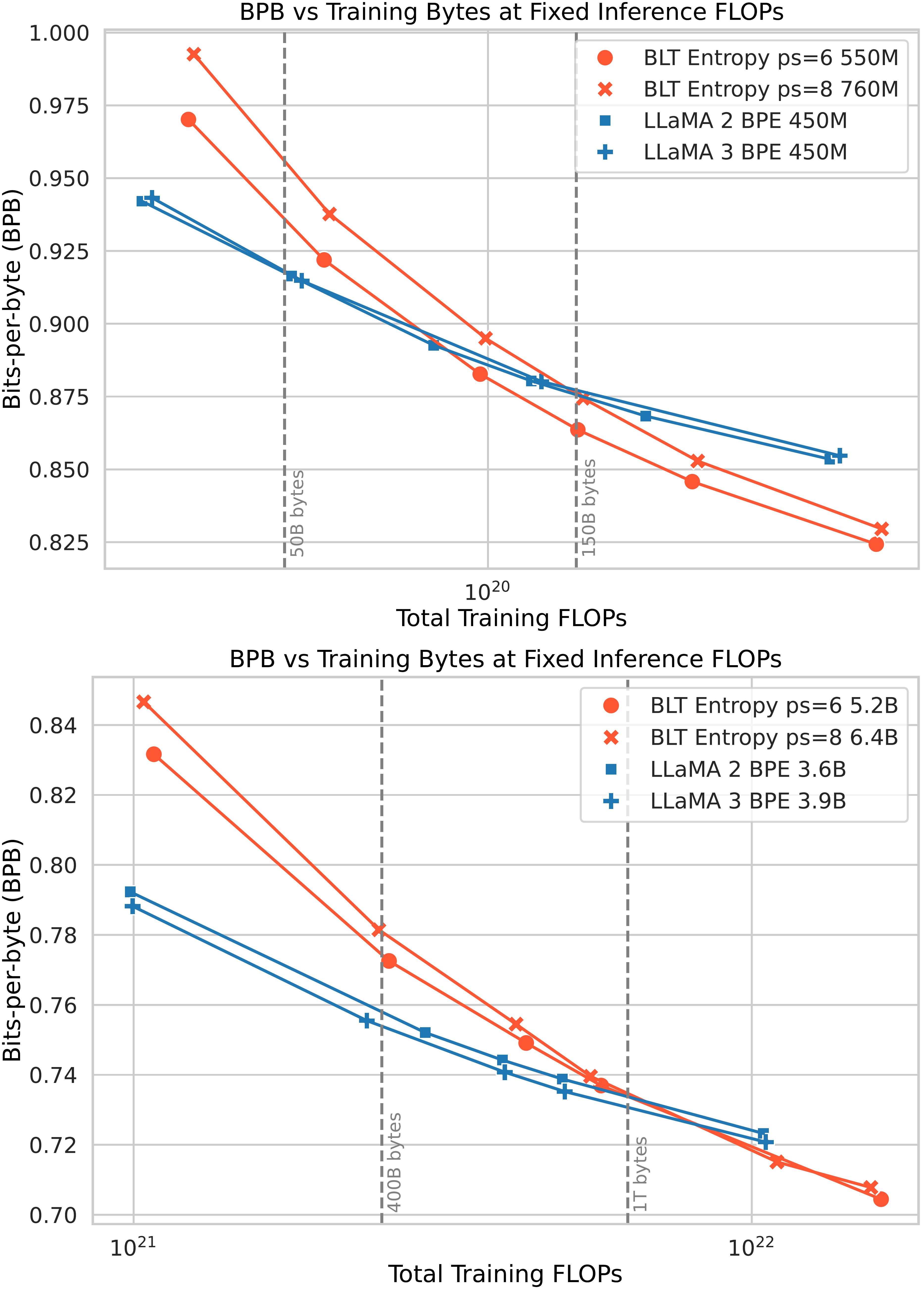
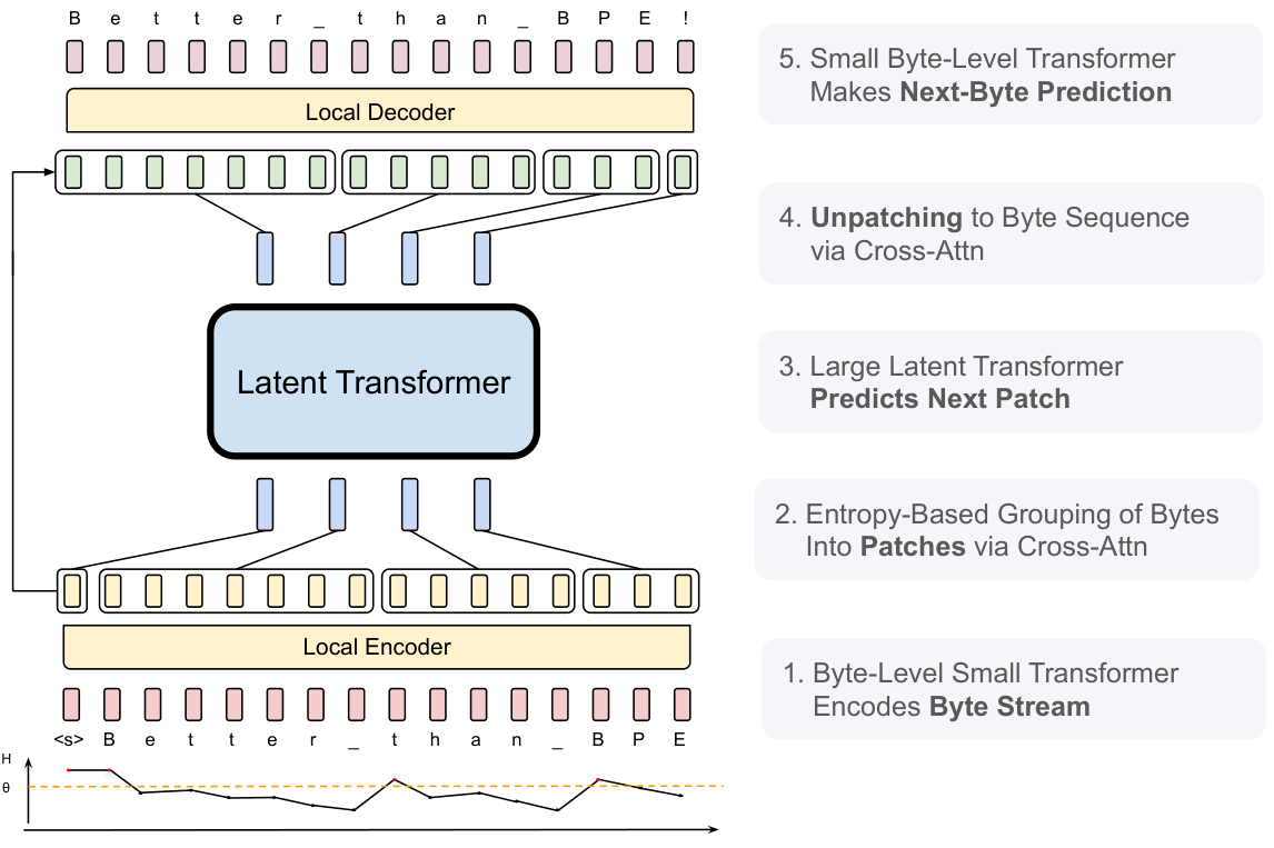
![**Figure 3:** Patching schemes group bytes in different ways, each leading to a different number of resulting patches. Since each patch is processed using a large transformer step, the number of patches directly determines the bulk of the compute expended in terms of $\textsc{flop}$ s. These schemes group bytes into patches by (a) striding every four bytes (§ 2.1) as in MegaByte ([10]), (b) tokenizing with Byte-Pair Encoding ($\textsc{bpe}$), in this case the Llama-3 ([11]) tokenizer, (c \& d) entropy-based patching as in this work (§ 2.3), (e) patching on space-bytes ([12]), (f) and patching on entropy using a small CNN byte-level model with 2-byte context.](https://ittowtnkqtyixxjxrhou.supabase.co/storage/v1/object/public/public-images/hp55vps8/patching_types.png)
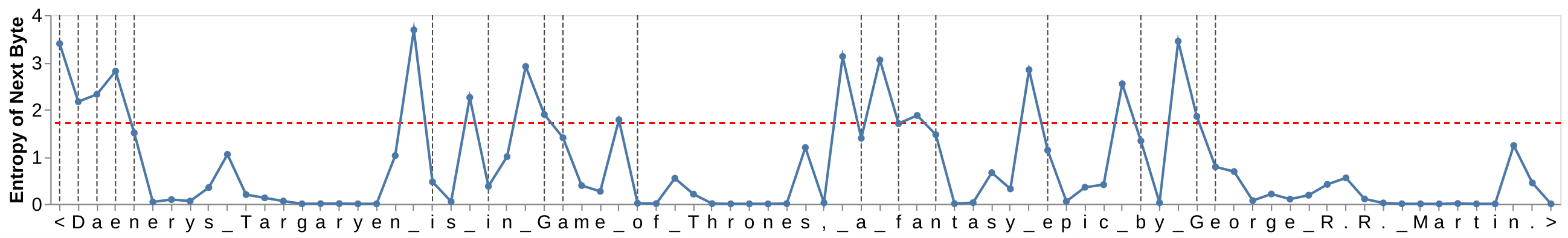
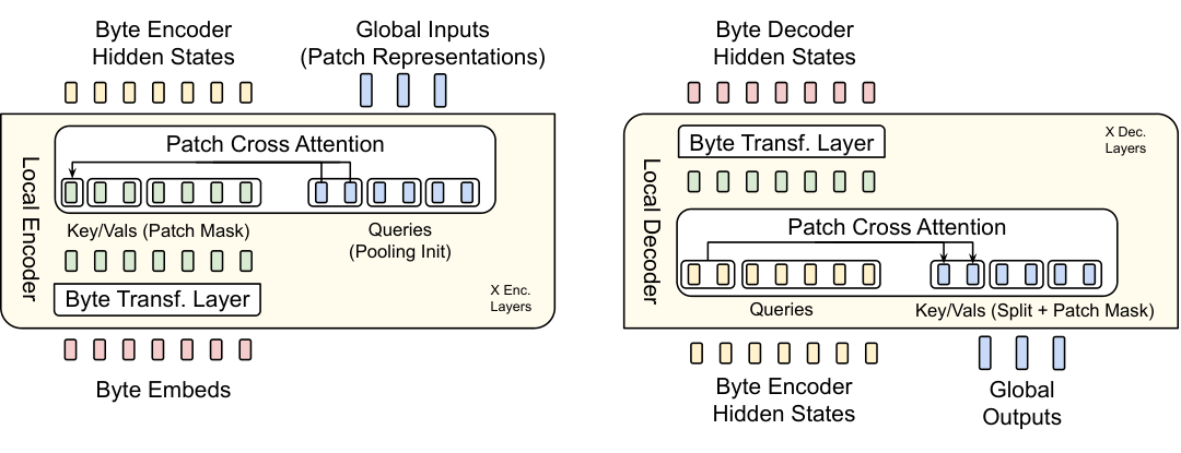
![**Figure 6:** Scaling trends for $\textsc{BLT}$ models with different architectural choices, as well as for baseline BPE token-based models. We train models at multiple scales from 1B up to 8B parameters for the optimal number of tokens as computed by [11] and report bits-per-byte on a sample from the training distribution. $\textsc{BLT}$ models perform on par with state-of-the-art tokenizer-based models such as Llama 3, at scale. PS denotes patch size. We illustrate separate architecture improvements on space-patching (**left**) and combine them with dynamic patching (**right**).](https://ittowtnkqtyixxjxrhou.supabase.co/storage/v1/object/public/public-images/hp55vps8/complex_fig_7d36d4e0d5f4.png)