ChapterPal

Log In Sign Up

Model Discovery Agent: LLM-assisted Bayesian experiment design for data-efficient discovery of mechanistic world models

Kevin Murphy
Dept. Computer Science
Univ. British Columbia, Canada

Abstract

Predicting the answer to interventional “what if” questions — the outcome of an action never taken — requires a mechanistic, causal model, not a curve fit; and learning such a model requires experiments, because passive data leaves its mechanisms unidentified. Experiments are expensive, so the central problem is data efficiency. We present the Model Discovery Agent (MDA), which couples a large language model (LLM), used as a proposer of candidate structures, with standard Bayesian machinery — sequential Monte Carlo (SMC) for parameter and structure posteriors, simulation-based inference (SBI) for intractable likelihoods, and value-of-information (VoI) for experiment design — to discover latent mechanistic world models from few interventions. MDA operates in the M-open setting: when the truth lies outside the current hypothesis class, a predictive check flags the inadequacy and the proposer expands the hypothesis space with a new model whose parameters are then identified by designed experiments. We show that discovery and design reinforce: the design step identifies the mechanism the discovery step proposes, and the identified mechanism improves predictions, enabling further discoveries from the remaining unexplained residuals. On three different benchmarks — covering physics (FORCEBENCH, (Wiemann et al., 2026)), chemistry (CHEMBENCH, (Kabra et al., 2026)) and biology (NEURONBENCH, a new partially observed single-neuron electrophysiology benchmark we create) — we show that MDA sets a new SOTA in terms of data-efficient model learning and reliable out-of-distribution prediction ability.

Executive Summary: Executive Summary

Predicting the effects of interventions—such as the outcome of a new drug, a novel spacecraft maneuver, or an untested neural stimulation protocol—requires mechanistic, causal models rather than statistical correlations. Passive observational data alone cannot distinguish among mechanisms that agree on seen behavior but diverge under perturbation. Experiments that resolve these ambiguities are expensive, making data-efficient discovery the central practical bottleneck. The Model Discovery Agent (MDA) addresses this gap by coupling large language models, used to propose candidate mechanisms, with standard Bayesian tools for inference and experiment selection.

The work sets out to demonstrate a practical system that discovers accurate mechanistic models from very few interventions, even when the true mechanism lies outside any initial hypothesis set, and to show that this yields reliable predictions on held-out interventional queries. MDA maintains a posterior over candidate structures and parameters via sequential Monte Carlo, uses value-of-information maximization to choose the next experiment, and employs predictive checks to expand the hypothesis space when residuals indicate that the current best model is inadequate. The same engine is applied without modification to three synthetic benchmarks spanning physics (force-law identification), chemistry (enzyme-kinetic rate laws), and neuroscience (single-neuron electrophysiology, including a new benchmark with partial observability and stochastic channel noise).

Across these domains, MDA reaches high predictive accuracy with roughly eight designed experiments, while pure LLM baselines require substantially more data to match performance and frequently recover numerically adequate but mechanistically incorrect expressions. On the physics benchmark MDA recovers the exact functional form in about three-quarters of runs and passes a normalized-error threshold in over 90 percent; on the chemistry tasks it improves symbolic accuracy from 42 percent to 56 percent relative to the prior state-of-the-art method while preserving mechanistic interpretability; on the neuroscience tasks the Bayesian forecaster with value-of-information design consistently outperforms both LLM and random baselines. The loop is self-reinforcing: informative experiments identify the proposed mechanism, the identified mechanism sharpens forecasts, and the improved forecasts expose subtler residuals that trigger further discovery.

These gains matter because they translate directly into lower experimental cost and faster time-to-insight in domains where each assay or trial is resource-intensive. They also produce interpretable models that support downstream decision-making under intervention, rather than opaque predictors. The results are robust across three distinct scientific fields and survive changes in the underlying language model, indicating that the Bayesian layer—not merely the proposer—drives the improvement.

The immediate next step is to move from synthetic benchmarks to closed-loop laboratory pilots on a narrow but real experimental system, using the same design–observe–update loop with automated or semi-automated hardware. Parallel engineering work should reduce the computational overhead of the inner sequential Monte Carlo steps and automate the learning of summary statistics for high-dimensional or stochastic observations. Further validation on physical (non-simulated) data and scaling to modestly higher-dimensional state spaces are required before broader deployment.

The reported gains rest on carefully constructed synthetic benchmarks whose noise models and design spaces are known; real-world measurement artifacts, unmodeled dynamics, and protocol constraints may narrow the advantage. Computational cost remains non-trivial for complex stochastic models. Within the tested regimes, however, the performance margin is large and consistent, supporting cautious confidence that the core architecture is sound.

1. Introduction

Section Summary: Many predictive models aim to answer "what if" questions about new actions or interventions, such as testing an untested drug or policy, but passive observations alone cannot distinguish between mechanisms that match the data yet behave differently under change. This requires building causal models of the underlying process, yet such models are typically underdetermined by observations, so experiments are essential but costly, creating a need for efficient ways to choose informative tests while generating new hypotheses. The Model Discovery Agent addresses this by using large language models to propose candidate mechanisms from domain descriptions and data, then applies Bayesian methods to select experiments that identify the best model, expanding the hypothesis space when predictions fail and demonstrating strong data efficiency on physics, chemistry, and biology benchmarks.

Much of what we want from a predictive model is interventional: not "what will happen?" but "what would happen if I did $a$?" (e.g., predicting the effect of administering a drug to a patient that it has never received, launching a probe on an orbit it has never flown, or deploying a policy never enacted before). Such interventional questions cannot in general be answered by a model fit to passive observation, however flexible: two mechanisms can agree on all observed data yet disagree under intervention. Answering interventional queries requires a mechanistic or causal model of the data-generating process ([3, 4]).[^2] Such mechanistic models are also the foundation of true scientific understanding ([5, 6, 7, 8, 9, 10]).

[^2]: Note that this paper is concerned with "level 2" causality, to use the terminology of Pearl's causal ladder ([3, 11]); this can be handled with standard decision-theoretic machinery ([12]), and does not need the more complex machinery required for "level 3" counterfactual reasoning ([13]).

Unfortunately, a latent mechanistic model is typically unidentifiable from observation alone: the passive data underdetermines it, and only intervening — perturbing the system and watching how it responds — breaks the degeneracy. But experiments are expensive (a lab assay, a clinical trial), which makes the operative problem data efficiency: identify the mechanism, well enough to answer the queries, in as few experiments as possible. This is the classical remit of Bayesian experimental design — choose the intervention whose outcome is most informative ([14, 15, 16]) — but it has rarely[^3] been combined with the open-ended hypothesis creation that scientific discovery demands.

[^3]: See Section 5 and Appendix G for discussion of related work.

To tackle these problems, we present the Model Discovery Agent (MDA). This uses a large language model (LLM), which contains useful prior knowledge ([17]), to propose candidate mechanisms, given a natural-language description of the domain and any initial observational data. We then combine this with standard Bayesian machinery: sequential Monte Carlo (SMC) for computing the posterior over parameters and structures and the model evidence, and value-of-information (VoI) maximization for choosing the next experiment. We extend the standard Bayesian machinery to the $\mathcal{M}$-open regime, where the true mechanism may lie outside the proposed hypothesis class ([18, 19]). We do this by testing if the current best hypothesis fails an out-of-sample predictive check; if so, we expand the hypothesis space (using the LLM), and then design an experiment to identify the new model's parameters (using VoI). We find that discovery and design reinforce each other: the experiment identifies the novel mechanism the proposal introduced, and the identified mechanism improves the model's forecasts, enabling the detection of ever more subtle predictive errors (c.f., ([20])).

We validate MDA on three sets of benchmarks, covering physics ($\textsc{ForceBench}$, based on ([1])), chemistry ($\textsc{ChemBench}$, based on ([2])) and biology ($\textsc{NeuronBench}$, a new single-neuron electrophysiology benchmark we create[^4]). In each case, we show that MDA is substantially more data-efficient than pure LLM baselines. In summary, we make 3 contributions: we develop the MDA method; we establish new SOTA performance on two existing interactive scientific discovery benchmarks; and we create a new benchmark ($\textsc{NeuronBench}$), which adds features such as partial observability and stochasticity that are missing in existing benchmarks.

[^4]: Benchmark available at https://github.com/murphyk/neuronbench

2. Problem statement

Section Summary: The section describes an agent that must learn about an unknown dynamical system, represented as a latent state-space model, by designing a limited number of experiments that apply inputs or interventions and then observing the resulting noisy outputs. It begins with an initial dataset from the unperturbed system and can run B additional trials, updating its beliefs after each one. Performance is evaluated by how accurately the agent predicts a target quantity on new, held-out test experiments drawn from a separate query distribution, using its final posterior beliefs to make forecasts.

Modeling assumptions.

We consider an agent interacting with an unknown "blackbox" dynamical system, that maps an optional sequence of inputs or control signals $x_{1:T}$, for $x_t \in \mathcal{X} \subset \mathbb{R}^{d_x}$, to a sequence of noisy observations, $y_{1:T}$, for $y_t \in \mathcal{Y} \subset \mathbb{R}^{d_y}$, in response to an optional perturbation or intervention $a \in \mathcal{A}$, and an optional setting of the initial condition of the system state $\iota \in \mathcal{Z} \subset \mathbb{R}^{d_z}$. WLOG, we assume the true data generating process can be represented by a latent-state dynamical system, or state space model (SSM), as shown in Equation 2. The latent dynamics (which may be deterministic or stochastic) are given by $z_{t+1}\sim p\big(z_{t+1}\mid z_t, , x_t; \mathrm{do}(a, \theta)\big)$, where $\mathrm{do}(a, \theta)$ represents the parameters of the system after applying intervention $a$.[^5] The noisy observation model is $y_t\sim p\big(y_t\mid z_t;, \theta\big)$, and the initial condition is given by $z_0\sim p(z_0\mid \iota)$. A static input-output system is a special case with $T=1$.

[^5]: We distinguish the intervention action $a$, as used in the causality literature, from the action sequence $x_{1:T}$, as used in the RL and control theory literature, because they play slightly different roles: the former changes the mechanism (parameters) of the underlying system, whereas the latter corresponds to changing the set of inputs or covariates applied to a fixed system. Of course, we can always define $x_0= a$, but we choose to keep them separate for notational clarity.

Data.

We define an experiment design as $\xi = (\iota, a, x_{1:T})$, where $x_t$ is the input at step $t$ (if present). If $\iota=[]$, it means the initial state of the system is chosen at random from some distribution $p(z_0)$. If $a=[]$, it means we use the original unperturbed system parameters $\theta$. The agent is presented with an initial dataset $\mathcal{D}0 = { (\xi_0^i, y{0, 1:T}^i): i=1:N_0 }$, where each sample is drawn from the system using $y_{0, 1:T}^i \sim p(\cdot| \xi_0^i)$, We assume the initial designs are from from the default (unperturbed or "wild-type") system, but they may use different input sequences $x^i$. The agent is then given a budget of $B$ turns to interact with the system. At each step, it designs an experiment $\xi_b$, and then collects data $y_{b, 1:T}$ from the environment, to create $\mathcal{D}b=(\xi_b, y{b, 1:T})$. It can use this knowledge to update its beliefs about the underlying model, $p_b = p(m | \mathcal{D}_{0:b})$, where $m$ specifies the SSM structure and parameters, and this belief can be used to design the next experiment.

Evaluation.

After $B$ rounds, each agent has the training set $\mathcal{D}\text{tr} = \mathcal{D}{0: B}$; the MDA agent also has its final belief state, $p_B$. When working with synthetically generated data, we can compare the agent's estimated model directly with the true model using an appropriate metric. In general, however, we score out-of-sample interventional prediction: we draw held-out test experiments $\xi\sim \mathcal{Q}$ from a query distribution $\mathcal{Q}$ (disjoint from the experiments the agent ran) and ask the agent to predict a target functional $F_q(y)$ of the outcome — the quantity the task actually cares about (in the simplest case $F_q=\mathrm{id}$, i.e. predict $y_{1:T}$ itself). Performance is the held-out loss

$ \mathcal{L} ;=; \mathbb{E}{\xi\sim \mathcal{Q}}\ \mathbb{E}{y\sim p^\ast(\cdot\mid \xi)} \big[, \ell\big(F_q(y), \ \hat{F}q(\xi)\big), \big], \qquad \hat{F}q(\xi)= \mathbb{E}{p(m, \theta\mid \mathcal{D}\text{tr})}!\big[F_q(Y)\mid \xi\big],\tag{1} $

where $p^\ast$ is the true system and $\hat{F}_q(\xi)$ is the agent's Bayes forecast — the posterior predictive of the target (see Appendix A.1 for details).

At a high level, our setup is a transductive problem similar to the ARC-AGI challenges[^6], except our domains use continuous-valued actions and observations, and are derived from real scientific problems.

[^6]: See https://arcprize.org/arc-agi. ARC-1 and ARC-2 are passive transduction problems, where $x^i$ is a 2d input grid (specified by the environment, not the agent) and $y^i$ is the resulting 2d output grid, and the goal is to learn $p(y_{\text{test}}| x_{\text{test}}, \mathcal{D}\text{tr})$, where $\mathcal{D}\text{tr}$ is a fixed set of 3 $(x, y)$ pairs. ARC-3 involves dynamic interaction with a 2d grid world, where the agent actively controls the sequence $x_{1:T}$ and observes $y_{1:T}$, which is more like our setting.

3. Methods

Section Summary: The MDA approach maintains a probability distribution over possible models of a system and iteratively refines it by running experiments. At each step it uses an LLM to propose new candidate models, evaluates how well each explains the data via sequential Monte Carlo sampling that automatically penalizes unnecessary complexity, and expands or prunes the set of hypotheses as needed. Experiments are then chosen to maximize expected information gain about which model is correct, after which the final posterior is used to forecast outcomes on new conditions.

Overview.

The MDA method is visualized in Figure 1a; see Algorithm 1 for detailed pseudocode. At each step, the agent updates its belief state $p_b=p(m| \mathcal{D}{0:b})$, which is a posterior distribution over models or hypotheses $m$. Then it chooses the next experiment by maximizing the expected value of information, $\xi{b+1}=\arg\max_{\xi \in \Xi} \text{VoI}(\xi)$. It runs the experiment and updates its dataset by appending $\mathcal{D}_{b+1}$. After $B$ rounds, the agent is asked to forecast the outcomes to some novel experimental conditions. We give the details below.

Sequential Bayesian inference.

The belief state $p_b=p(m| \mathcal{D}{0:b})$ is a posterior over models $m$, represented as a set of $N_m$ particles. Each model $m$ encodes the structure of the system, as in a structural causal model (SCM) ([3]). This posterior is updated using Sequential Monte Carlo (SMC), following the ModelSMC method of ([23]) and SMC-S method of ([24]); see Algorithm 3 for the pseudocode. We use an LLM to propose a new model given the set of previous hypotheses, their corresponding residual errors (derived from the data), and an initial text prompt (context) $\mathcal{C}$. We denote this proposal distribution by $p(m_b|{m{b-1}^n}, \mathcal{D}_{0:b})$.

After proposing a new model (particle), we evaluate its evidence (marginal likelihood), $Z_m = p(\mathcal{D}{0:b}|m) = \int p(\mathcal{D}{0:b}|m, \theta), p(\theta|m), d\theta$, using the adaptive-tempered SMC method shown in Algorithm 4. (See ([25, 26]) for more details.) Crucially, the integration over model parameters provides an automatic Occam penalty factor for complex models with many parameters ([27]). Thus, over the course of inference, we will get a set of hypotheses that tradeoff complexity with model fit, as shown in Figure 1b.

Likelihood functions.

To compute the likelihood, $p(\mathcal{D}{0:b}|m, \theta)=\prod{i \in \mathcal{D}{0:b}} p(y{1:T}^i| \xi^i, m, \theta)$, we consider two strategies. If the latent dynamics are a deterministic function of the initial conditions, $z_0$, then we can use $p(y_{1:T}|z_0, m, \theta) = \prod_{t=1}^T p(y_t|z_t, m, \theta)$ where $z_t = m^t_{\theta}(z_0)=m_{\theta}(\cdot s(m_{\theta}(z_0)))$ is $z_0$ pushed through the forwards model $t$ times. If the latent dynamics are stochastic, we can use the particle filter method of Algorithm 5 to approximate $p(y_{1:T}|z_0, m, \theta) = \int \prod_t p(y_t|z_t, m, \theta) p(z_t|z_{t-1}, m, \theta) d z_{1:T}$.

For some problems (such as $\textsc{NeuronBench}$), individual trajectories are very noisy, so a per-time step likelihood $p(y_t|z_t)$ is not meaningful. In such cases, we convert the trajectory into a set of global summary statistics, $s_j(y_{1:T})$, and use a trajectory-level likelihood of the form $p(y_{1:T}|m, \theta) = \prod_{j=1}^J p(s_j(y_{1:T})|m, \theta)$, as is standard in the simulation based inference literature ([28]). In Appendix A.4 we present some initial results on learning these summary statistics $\text{vs.}(y)$ as well as the model itself.

Expanding and shrinking the hypothesis space.

SMC can update the posterior over hypotheses (models) given observations. However, in the $\mathcal M$-open case ([18, 19]), we may need to expand the hypothesis space to account for a novel mechanism. To do this, we use a predictive check, i.e., a held-out interventional forecast (c.f., ([19])). If the error is too large, MDA expands the hypothesis space by prompting the LLM to suggest a novel unnamed mechanism (which is endowed with broad ("uninformative") priors). (This is analogous to the Breaker–Builder method of ([20]), and is how MDA can create new knowledge, overcoming a limitation of pure LLM-based discovery ([29]).) Conversely, if the posterior has confidently identified a model that fits well, we reduce the number of hypotheses, to prevent a proliferation of near duplicates, which diminishes performance. See Appendix A.2 for more details on MDA's meta-controller.

Experiment design.

We choose the experiment whose outcome is most informative about which hypothesis is true: $\xi^\star=\arg\max_{\xi \in \Xi} I(M;Y_\xi\mid \mathcal{D})$ ([14, 30, 15, 16]). This is called the Value of Information (VoI) for an experiment. For the case of deterministic latent dynamics, and Gaussian observation noise, we can derive a simple analytic expression for the VoI, shown in Equation 9. This picks the design with highest posterior-predictive variance of the outcome. Since the per-structure parameter posteriors are usually fairly concentrated, this variance is dominated by cross-model disagreement. We can optimize the VoI for small design spaces by simply enumerating each choice and scoring it. For larger continuous spaces, we use CMA-ES ([31]). As baselines, we also consider random designs and LLM-proposed designs (as in ([32, 1])).

Prediction.

Once we have accumulated the full dataset $\mathcal{D}{0: B}$, and created the posterior over hypotheses, $p_B=p(m| \mathcal{D}{0: B})$, we evaluate the model in terms of its ability to forecast the outcome of novel experiments. For simplicity, we focus on predicting the posterior mean of each scalar output, $E[Y\mid \xi, \mathcal{D}_{0: B}, p_B]$, which is optimal when using $\ell_2$ loss. We consider 3 methods:

• Bayes-forecast, $E[Y\mid \xi, \hat{m}]$ with $\hat{m}=\arg\max_m p_B(m)$ being the MAP model.[^1]
• LLM-forecast, $E[Y\mid \xi, \hat{m}]$ with $\hat{m}=\mathrm{LLM}(\mathcal{D}_{0: B})$ being an LLM-generated model, created using standard code synthesis methods. (This is the approach used in ([1]).)
• ICL-forecast, $E[Y\mid \xi, \mathcal{D}_{0: B}]$: this is an in-context LLM-based predictor that conditions on the collected data and directly predicts the expected output, without using any kind of explicit model (c.f., ([33])).

[^1]: In general, the Bayes-forecast can use the full Bayes model average $E[Y\mid \xi, \mathcal{D}{0: B}, p_B]$, as proposed in ([34]). For example, suppose we want to predict the expected number of neuron spikes $\ell_2$ at input current level $E[Y\mid \xi, \hat{m}]$, as required in $\textsc{NeuronBench}$ discussed in Section 4.3, where $\hat{m}=\arg\max_m p_B(m)$ is specified as part of the experiment design $E[Y\mid \xi, \hat{m}]$. The posterior mean can be approximated from the weighted set of particles using $\hat{m}=\mathrm{LLM}(\mathcal{D}{0: B})$, where $E[Y\mid \xi, \mathcal{D}{0: B}]$ is the number of spikes in trace $B{\le}8$, and $f{\text{design}}$ is the deterministic ouput of running model $f_{\text{predict}}$ with parameters $+$ on input $+$.

4. Experimental results

Section Summary: The experimental results show that the MDA approach, which combines value-of-information experiment design with Bayesian forecasting, learns accurate predictive models from far fewer trials than either random selection or pure large-language-model agents across synthetic benchmarks in physics, biology, and chemistry. In a standardized loop of at most eight experiments, each method proposes the next trial, updates its model, and is scored on how well it forecasts held-out outcomes; MDA consistently drives this error down faster. On the ForceBench suite of particle force-law discovery tasks, the advantage appears both in lower normalized mean-squared error and in a higher fraction of runs that reach an acceptable accuracy threshold, with the method’s preference for maximally informative long-range probes illustrated in a Yukawa-force example.

In this section, we summarize some our our experimental results on various benchmarks from physics, biology and chemistry (see Table 3). We show that the MDA method reduces held-out interventional predictive error much faster (in terms of number of experiments) than the baselines. We give more details in Appendix C, Appendix D and Appendix E.

Common protocol.

Every benchmark is run through the same design loop for $B{\le}8$ experiments. At each step the agent selects the next experiment with a design function $f_{\text{design}}$ — random, LLM-proposed, or Bayesian VoI — and after each step we forecast held-out interventional outcomes with a forecaster $f_{\text{predict}}$ (Bayes-, LLM-, or ICL-forecast; Section 3) and score them by mean-squared error against the ground truth. We report this held-out error as a function of the number of experiments; because all datasets are synthetic and the true model is known, in some domains we additionally check whether the recovered model is symbolically equivalent to the truth. The two canonical agents are "MDA" (VoI design $+$ Bayes-forecast) and the "LLM agent" (LLM design $+$ LLM-forecast).

4.1 ForceBench: discovering force laws

Benchmark.

In this section, we give a brief description of $\textsc{ForceBench}$, which is our wrapper on top of the $\textsc{DiscoverPhysics}$ benchmark from ([1]). (We do not change the underlying benchmark, merely the interface, to make it compatible with our other benchmarks.) $\textsc{ForceBench}$ requires an agent to infer an unknown but novel force law governing the behavior of two or more particles in a 2d space. The agent can control the initial location and velocity of one of the particles, as it is launched, as well as a few other environment parameters. (In practice we discretize the design space into a fixed menu of 13 different combinations, listed in Table 5.) The performance of the learned model is assessed on a test set which probes the model's predictive performance in novel experimental settings beyond the training set. Following the paper, we report this in terms of the normalized MSE, (nMSE $=$ MSE $/$ test-trajectory variance). See Appendix C.1 for further details.

Modeling assumptions.

The agent assumes the unknown force can be represented as a Green's function $F$, and asks the LLM to propose various candidates (see Appendix H for details of the prompt). It then derives the acceleration using Newton's law, and integrates this to get velocity, and then integrates this again to generate the trajectory. It assumes the likelihood $p(y_{1:T}| \xi, F, \theta)$ is Gaussian, as in Equation 4, and then does posterior inference over $F$ and experiment design following the MDA recipe.

Data efficiency experiments.

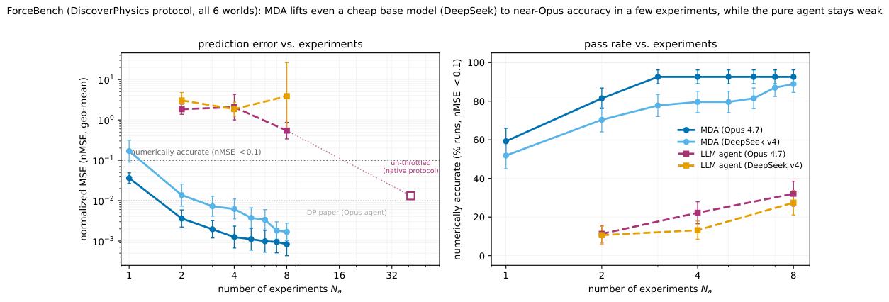
In Figure 2, we show the performance of MDA vs the baseline LLM agent aggregated over all six of the two-particle worlds (see Figure 8 and Figure 9 for the performance plots for all 11 worlds). For each of the 6 worlds, we sample 3 random initial conditions, and roll out 3 trajectories per IC. Both agents use the same design space, and for the LLM they either use Opus 4.7 (the best model reported in ([1])) or the cheaper DeepSeek-v4 Pro. On the left we plot the nMSE of the forecast for up to $B=8$ steps.[^7] On the right we plot the fraction of runs where the prediction "passes", following the paper's definition of a pass as nMSE $\leq 0.1$. (We exclude the paper's textual explanation criterion as part of the definition of "pass" because we found it to be unreliable; see Appendix C.7 for discussion.) From both plots we see that MDA is substantially more data efficient than the LLM baseline, and that Opus is better than Deepseek. See Table 8 for a list of the laws discovered by each agent after $B=8$ experiments.

[^7]: For the Opus LLM baseline, we also run their agent in its native "unthrottled" mode, in which it performs multiple experiments per step. Thus 16 rounds of their agent performs $\sim 41$ experiments on average. The nMSE of 0.013 we get using this method matches the 0.01 reported in their paper, validating our experimental pipeline.

Example: Yukawa world.

As a concrete example, we consider $\textsc{yukawa}$ world, whose force law has the form $F = q_i q_j K_1(r/\lambda)/\lambda$, where $K_1$ is the modified Bessel function and $\lambda=2$. The agent can choose the initial launch radius $r_0$ and speed $v_0$ of the target particle. The screened kernel $K_1(r/\lambda)/\lambda$ and the power laws that fit its short-range behaviour are nearly identical for $r\le\lambda$ and diverge only at longer range (where the screening has decayed), so a probe must reach past the screening length to break the tie: a short-range launch leaves the candidate trajectories indistinguishable, while a long-range launch makes the true Yukawa fan out from its near-misses (visualized in trajectory space in Figure 15, Appendix C). By maximizing the VoI, the agent therefore designs long-range probes.

The effect of the long range experiment triggers an "aha" moment for the agent. This is visualized in the Pareto curve in Figure 1b which plots models on the accuracy–complexity frontier. With only short-range data, the true kernel sits mid-frontier with no edge over its near-misses; only after an informative long-range probe is added does the frontier shift down, making the true model drop to the convex corner — the moment where the agent truly "groks" the concept. (Note that the $x$-axis in Figure 1b is a Bayesian description length, $-\log_2 p(m\mid \mathcal{D})$ — the posterior code-length of each candidate law. Unlike a purely syntactic complexity, such as the Halstead metric used in ([35]), this is data-dependent: it rewards a law only to the extent the evidence supports it.)

4.2 ChemBench: discovering enzyme-kinetic rate laws

Benchmark.

In this section, we briefly describe $\textsc{ChemBench}$, which is our wrapper on top of $\textsc{ActiveSciBench-Chem}$ from ([2]). (We don't change the underlying benchmark, just the interface, to make it compatible with our other benchmarks.) The problem is to learn a function mapping seven controllable inputs (substrate, inhibitor, second substrate and product concentrations, enzyme loading, temperature and pH) to a reaction rate $r$: $ r = f\big(C_A, C_I, C_B, C_P, \mathrm{Enz}, T, \mathrm{pH};, \theta\big)$. See Table 1 for some examples. The experimenter gets to set the 7 input variables, $\iota= x_0$, and observes the scalar response. Note that this problem is a special case of our SSM setup, since there is no temporal evolution. Following the paper, We measure performance using the held-out root-mean-squared log-error (RMSLE). If this is below $\epsilon{=}0.01$, we say the law is "numerically exact". We also check for symbolic equivalence with the truth (which they call Structural Accuracy) using sympy. See Appendix D.1 for further details.

Modeling assumptions.

The agent assumes the unknown function $f$ can be represented as an algebraic equation, and asks the LLM to propose various candidates (see Appendix H for details of the prompt). It assumes a Gaussian likelihood with multiplicative noise, $p(y| \xi, f, \theta)= \mathcal{N}!\big(y \mid f(\xi, \theta), \ \sigma_{\mathrm{rel}}, f(\xi, \theta)\big)$, to match the benchmark's noise model, and its RMSLE metric. Given this model, the agent does posterior inference over $f$ and experiment design following the MDA recipe.

VoI optimization.

MDA by default uses VoI to pick the design. However, following ([2]), we also create a baseline which we call $\textsc{MDA (Mean)}$, which picks the design of highest posterior-mean rate — an exploit/peak-seeking acquisition, as in Bayesian optimisation — rather than the most model-discriminating one: $\xi^\star_{\mathrm{mean}} = \arg\max_{\xi\in \Xi}\ \mathbb{E}_{m, \theta\mid \mathcal{D}}!\big[r(\xi;m, \theta)\big].$ Both designs are one-step (myopic); they differ only in the objective — exploit the predicted rate versus discriminate between mechanisms. We maximise either objective over the continuous $7$-D design box $\Xi$ in one of two ways: by Monte-Carlo (draw $n_c{=}48$ candidate designs — log-uniform on the concentration/enzyme axes, uniform on $T$ /pH — and take the argmax) or with CMA-ES ([31]) over the box at the same $48$ objective evaluations. We find the latter method is significantly better, so we use it by default.

Data efficiency experiments.

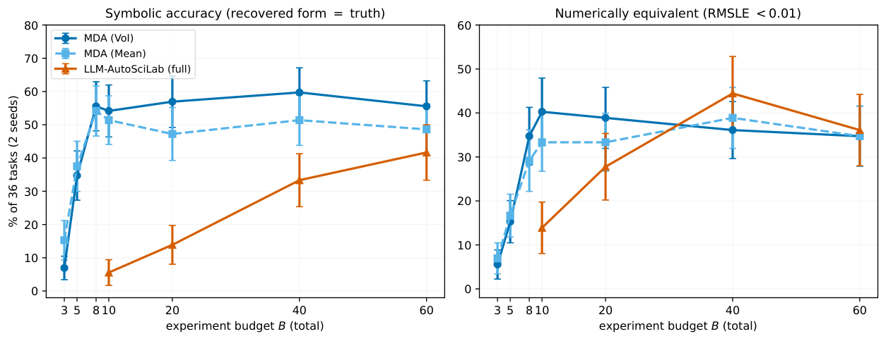
In this section, we compare MDA to $\textsc{LLM-AutoSciLab}$ from ([2]), which was the previous SOTA on this benchmark. Following their experiment protocol, we use a stratified $36$-task subset ($12$ domains $\times$ easy/medium/hard) at two seeds. Figure 3 shows the data efficiency learning curves, which show that MDA is far more sample-efficient: it reaches its ceiling within about $8$ experiments (overall SA ${\approx}56%$), whereas $\textsc{LLM-AutoSciLab}$ only reaches SA $\approx 42%$ by $B=60$.[^8] See Appendix D.2 for more results.

[^8]: Our result of $42%$ SA is higher than the $35.1%$ SA score they report in their paper, because we replaced their use of gpt-4o-mini with Opus 4.7, to be comparable to MDA. Note, however, that we stick to Qwen2.5-7B for the adaptive ensemble used by their code. (We also verified that dropping this ensemble component substantially hurt performance of their method.)

lt;0.01$; the head-to-head Table 9 additionally reports the released benchmark's own looser $0.05$ threshold, for comparability with its published numbers). MDA (VoI) rises to its ceiling within ${\sim}8$ experiments and leads on symbolic accuracy at every budget; $\textsc{LLM-AutoSciLab}$ only catches up by $B=60$. On numerical accuracy, $\textsc{LLM-AutoSciLab}$ catches up sooner, but this is because of overfitting (see Table 1).">

Example.

Table 1 shows the laws recovered on three representative domains. MDA returns interpretable mechanisms — exactly the true form for substrate inhibition, and the correct inhibition/saturation structure elsewhere (although sometimes with a spurious extra factor). $\textsc{LLM-AutoSciLab}$ 's PySR instead returns numerically-fit but mechanistically meaningless expressions — nested $10^{, a\log(\cdot)}$ and stretched-exponential forms — that can score a low RMSLE (even $0.001$ on the hard noncompetitive domain) while being symbolically wrong: the high-exact/low-symbolic pathology discussed in ([2]).

\begin{tabular}{@l l l l@}
\toprule
Domain & True law & MDA recovers & \textsc{LLM-AutoSciLab} recovers \\
\midrule
substrate inhib. (easy)
   {} & $\dfrac{k\, \mathrm{Enz}\, C_A}{K_m{+}C_A{+}C_A^2/K_i}$
   {} & \emph{same form} \checkmark ($.007$)
   {} & $\mathrm{Enz}\, (a\, r^{C_A}{+}\dots)$ $\times$ ($.23$) \\
noncompetitive (hard)
   {} & $\dfrac{k\, \mathrm{Enz}\, C_A}{(1{+}C_I/K_i)(K_m{+}C_A)}$
   {} & Hill ${\times}$ noncomp. $\approx$ ($.018$)
   {} & $10^{\, 0.87\log(0.5\sqrt{\mathrm{Enz}/(C_I{+}\cdot)})}$ $\times$ ($.001$) \\
Michaelis--Menten (easy)
   {} & $\dfrac{k\, \mathrm{Enz}\, C_A}{K_m{+}C_A}$
   {} & ${+}$ spurious $e^{-E_a/RT} \approx$ ($.017$)
   {} & $10^{\, 0.43\log(\mathrm{Enz}\, T^{0.37}/\cdot)}$ $\times$ ($.015$) \\
\bottomrule
\end{tabular}

4.3 NeuronBench: discovering ion-channel mechanisms

Benchmark.

We design a new benchmark, $\textsc{NeuronBench}$, by creating 6 "mystery neurons", based on the generalized Hodgkin-Huxley (HH) model, which are a set of nonlinear ODEs for describing the spiking behavior of neurons (see Appendix E.2 for details of HH models). Each mystery neuron has incoming current represented by $I_{\mathrm{Na}} + I_K + I_L + I_{\mathrm{Z}}$, where Na is the sodium channel, K is the potassium channel, L is the leak channel, and $Z$ is a novel membrane mechanism that we design, in order to prevent the LLM from simply recalling the model from memory (in most worlds an added channel, but in one a modification of the existing Na$^+$ channel rather than a new current). The experimental protocol allows the agent to specify the input signal (an electrical current) over time. We assume this is chosen from a set of 9 templated signal shapes. In addition, the agent can optionally apply 3 different kinds of ion channel blockers that change the underlying mechanism (see Appendix E.3 for details). So the total design space has $9 \times 4 = 36$ discrete options.

Modeling assumptions.

The agent assumes the data can be represented by some kind of HH model $m$, and asks the LLM to propose various candidates (see Appendix H for details of the prompt). It then converts this into an ODE that defines the deterministic dynamics $p(z_t|z_{t-1}, x_t)=\delta(z_t = m(z_{t-1}, x_t;\theta))$, where the latent state is $z_t=\big(V(t), \ \text{gating variables }\big)$ defined in Equation 19b. Finally it integrates this ODE over time to get a candidate trajectory $z_{1:T}$ from which the noiseless voltage trace $V(1:T)$ can be extracted. However, rather than evaluating the ability of the model to exactly match an observed trace (which can be very "wiggly" and hard to predict, even in the deterministic regime), we reduce the trace to a summary statistic $s$, and use a synthetic likelihood ([28]) of the form $p(s(y_{1:T})| \xi, m, \theta)$. For example, if $s(y)$ is the number of spikes in the trace $y$, we can use the Poisson likelihood $p(s(y_{1:T})| \xi, m, \theta)$ in Equation 24. We then do posterior inference over $m$ and experiment design following the MDA recipe.

Data efficiency experiments.

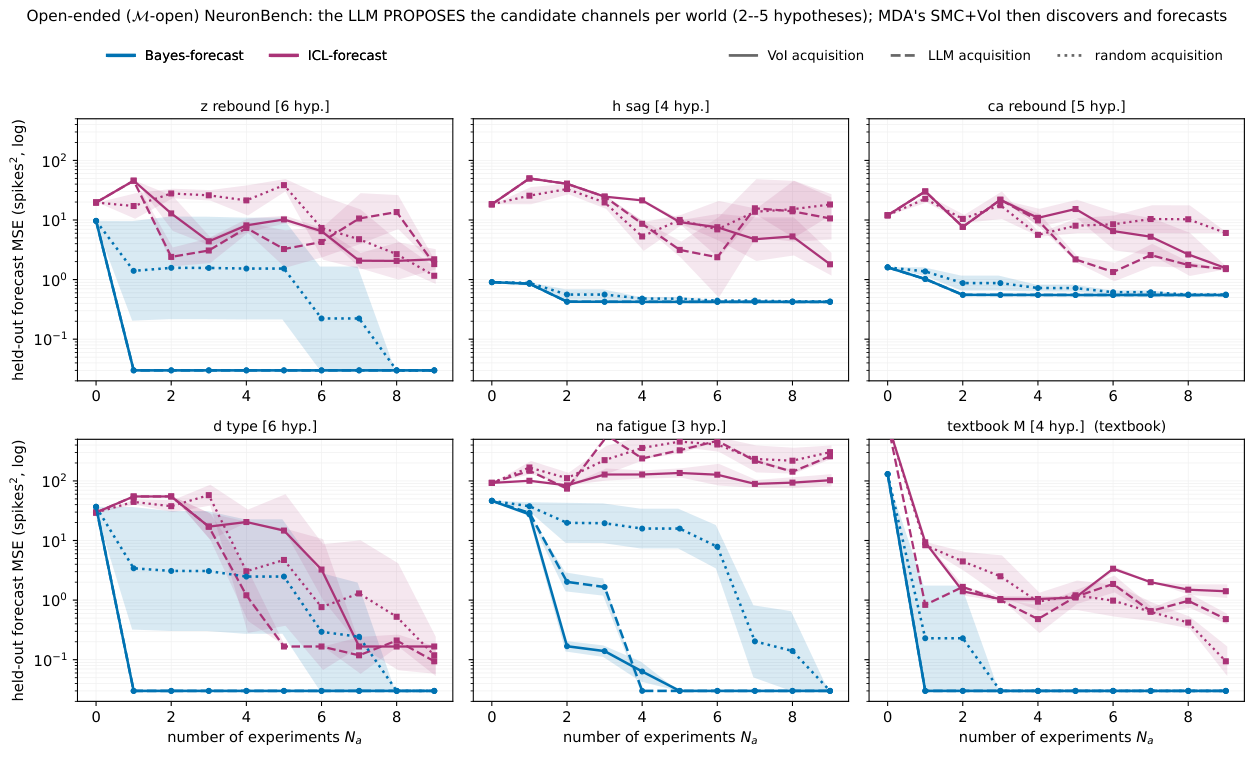
In Figure 4, we show test error vs number of experiments for all six worlds. For each world the LLM is shown only the phenotype (the observable signature, not the mechanism) and proposes $2$ – $5$ candidate channels, which we map onto a shared channel library; the truth is sometimes not proposed — e.g. on $\textsc{z-rebound}$ the LLM omits the low-threshold inward current — a genuine $\mathcal{M}$-open miss that we keep representable so the residual can reopen the pool. MDA then runs Poisson-evidence selection over that pool with VoI-designed experiments. We see that the Bayes-forecaster (blue) is significantly better than the in-context forecaster (purple) on every world; and within the Bayes-forecaster family, VoI and LLM-proposed experiment design perform similarly and both beat random design.

Stochastic extension.

The worlds above use a deterministic Hodgkin–Huxley forward model, which can be represented by a deterministic ODE, so the likelihood is closed-form. In Appendix F.1 we make the latent dynamics stochastic (by adding finite-channel gating noise), turning the model into an SDE. We call this benchmark $\textsc{NeuronBenchStoch}$. The corresponding likelihood $p(y\mid \xi, m, \theta)$ is now intractable — the one regime none of our other benchmarks reach. In Appendix F.1, we show that a deterministic likelihood gives poor results (the method confidently selects the wrong model), whereas a particle filter approximation to the marginal likelihood (Algorithm 5) gives the correct results. Unfortunately running a particle filter inside the tempered SMC algorithm (needed to compute the evidence) — which is in turn nested inside of the SMC algorithm over models — is very slow. Fortunately we show that we can learn a suitable summary statistic function (using a 1d convolutional neural network), which speed things up by $\sim 10^4\times$. Furthermore, because the summary is learned, this simulation-based likelihood adapts to whatever mechanisms the LLM proposes, rather than needing a hand-crafted feature per hypothesis.

5. Related work

Section Summary: This section reviews prior research on using causal models to answer hypothetical intervention questions, along with methods for selecting informative experiments and performing inference when exact calculations are difficult. It also discusses recent applications of large language models to generate scientific hypotheses through both static data analysis and active experimentation, highlighting differences in how the current work manages uncertainty and diverse domains. Finally, it describes existing benchmarks for agents that discover scientific laws via interactive experiments and notes the new contributions built on top of them.

• Causal models for interventional prediction. Predicting "what if" questions using causal models is discussed at length in ([3]). Recently [4] proved that an agent that can robustly predict across a full range of interventions (distribution shifts) must have implicitly learned a causal world model. We instead explicitly represent the causal model, so that we can leverage prior knowledge from LLMs ([17, 36]), reason over our uncertainty using Bayesian methods, and provide an interpretable model to the user.
• Bayesian experimental design. Choosing the most informative experiment is the classical model-discrimination objective of ([14]), reviewed in ([15, 16]); modern work scales it with amortised and gradient estimators ([37]).
• Simulation-based inference. When the likelihood is intractable, SBI learns it or the posterior from simulations ([38]), and learned/embedding summary statistics are a whole subfield of their own ([39, 40, 41, 28]).
• LLMs for scientific discovery. LLMs have been used to propose scientific hypotheses in many papers, including from static datasets ([42, 23, 35, 43, 44]) as well as actively collected datasets from agent-designed experiments ([24, 45, 21, 46, 47]). Our work is in the latter camp, differing mainly in how we handle the $\mathcal M$-open regime inside SMC, the diversity of domains, and by the fact that we beat SOTA methods based on LLMs.
• Benchmarks for interactive scientific discovery. Various benchmarks evaluate agents that learn scientific laws by interactive experimentation: we build on $\textsc{DiscoverPhysics}$ ([1]) and $\textsc{ActiveSciBench-Chem}$ ([2]), add our own $\textsc{NeuronBench}$, and may target others such as $\textsc{NewtonBench}$ ([48]) in the future.

Appendix

Section Summary: The appendix elaborates on a state-space modeling framework for unknown dynamical systems, in which latent states evolve over time under fixed mechanisms that interventions can alter, while producing noisy observations. It derives likelihoods assuming Gaussian noise, explains how summary statistics can replace raw high-dimensional data for tractable inference, and shows how models are scored on held-out test experiments using Bayesian predictions. The text also sketches the MDA inference procedure, which iteratively selects experiments, updates posteriors over models via sequential Monte Carlo, and adds fresh hypotheses when existing ones leave large unexplained residuals.

A. Method: further details

A.1 Modeling assumptions

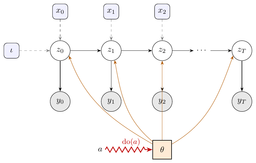
We assume the unknown dynamical system is represented by a state space model, as shown in Equation 2. This corresponds to the following probabilistic model $m$:

$ z_{t+1}\sim p\big(z_{t+1}\mid z_t, , x_t; \mathrm{do}(a, \theta)\big), \qquad y_t\sim p\big(y_t\mid z_t;, \theta\big), \qquad z_0\sim p(z_0\mid \iota).\tag{2} $

where $\mathrm{do}(a, \theta)$ represents the parameters of the system after applying intervention $a$. An experiment design $\xi$ (the choice of initial conditions and control knobs the agent selects) fixes the induced intervention $a$; we therefore write $\mathrm{do}(\xi)$ for the intervened system when the design is the decision variable, as in the VoI objective below. The SSM assumption is without loss of generality, since any non-Markovian model can be converted to Markov form, as long as the latent state space is allowed to grow.

Likelihoods.

If we assume the observation model just adds Gaussian noise, the $z$-conditioned likelihood becomes

$ p(y_{1:T}|z_{0:T}, m, \theta) = \prod_{t=1}^T \mathcal{N}(y_t|z_t, \sigma^2)\tag{3} $

Marginalizing out the latent variables gives

$ p(y_{1:T}|m, \theta) = \int p(s(y_{1:T}) | z_{1:T}, m, \theta) p(z_{1:T} | m, \theta) d z_{1:T} $

If the latent dynamics are deterministic, then $z_t=m^t(z_0;\theta)$, where $m^t$ is the forwards model iterated $t$ times, so this simplifies to

$ p(y_{1:T}|z_{0}, m, \theta) = \prod_{t=1}^T \mathcal{N}(y_t|m^t(z_0;\theta), \sigma^2)\tag{4} $

Summary statistics.

For simple problems we can ask how well the model predicts the entire observed trajectory, $y_{1:T}$, and measure its performance using a Gaussian likelihood, as above. But for more complicated signals, like a neural voltage trace, it is common to replace the raw data $y_{1:T}$ with a summary feature vector $s(y_{1:T})$ and to replace $p(y_{1:T}|m, \theta)$ with $ p(s(y_{1:T})|m, \theta)$. (We discuss how to learn the summary function in Appendix A.4.) If the features are uncorrelated, and the latent dynamics are deterministic, we can use this factorized form:

$ p(y_{1:T}|m, \theta) \propto p(s(y_{1:T})|m, \theta) = \prod_{j=1}^J p_j(s_j(y_{1:T}) | m, \theta)\tag{5} $

In general, the model may have stochastic latent variables, so we need to compute

$ p(s(y_{1:T})|m, \theta) = \int p(s(y_{1:T}) | z_{1:T}, m, \theta) p(z_{1:T} | m, \theta) d z_{1:T}\tag{6} $

If $s(y_{1:T})=y_{1:T}$, we can use particle filtering (Algorithm 5) to compute this pathe intregral; in particular, PF sequentially estimates the posterior $p(z_{1:T}|y_{1:T}, m, \theta)$ and its corresponding normalization constant $Z = p(y_{1:T}|m, \theta)$. In general, the summary statistic is not the identity function and does not factorize over time, so we cannot use PF, but we can use SBI methods which we discuss in Appendix A.4.

Summaries, queries, and the held-out loss.

Held-out test experiments are drawn from the query distribution $\xi\sim \mathcal{Q}$, disjoint from the agent's own designs. Given $\mathcal{D}_\text{tr}$, the agent is evaluated using

$ \mathcal{L} ;=; \mathbb{E}{\xi\sim \mathcal{Q}}\ \mathbb{E}{y\sim p^\ast(\cdot\mid \xi)} \big[, \ell\big(F_q(y), \ \hat{F}q(\xi)\big), \big], \qquad \hat{F}q(\xi)= \mathbb{E}{p(m, \theta\mid \mathcal{D}\text{tr})}!\big[F_q(y)\mid \xi\big],\tag{7} $

where $p^\ast$ is the true system and $\hat{F}q(\xi)$ is the agent's Bayes forecast. Note that $F_q(y)$ is what the agent gets evaluated on, but $s(y)$ is the summary statistic it uses for inference. Typically we have $\dim y \ge \dim s(y) \ge \dim F_q(y)$. For example, in $\textsc{NeuronBench}$, $y$ is the raw voltage trace, $s(y)$ is a vector of 6 summary features, and $F_q(y)=n\text{test}$, the test-window spike count.

A.2 Inference algorithms

In this section, we give pseudocode for the main algorithms.

MDA outerloop.

The MDA algorithm, illustrated schematic in Figure 6 is defined more precisely in Algorithm 1. It is a fairly standard sequential Bayesian experiment design loop. It uses an SMC subroutine to update the posterior over models $p(m| \mathcal{D}_{0:b})$ after obtaining $\mathcal{D}_b$ from the $b$ 'th experiment. However, it adds two novelties, both of which turn out to be important for good performance in challenging domains (see Figure 17).

• It handles the M-open setting, in which we prompt the LLM to consider new hypotheses (beyond the current set of particles) if the residual error $r^*$ of the current best (MAP) model, $m^*$, is above a threshold $\tau_r$. (This can happen if the agent receives an informative but surprising observation.) In practice we do this by setting $R_m$ to $R_{\max}>0$; this enables $R_m$ rounds in which we propose a batch of $N_{\mathrm{new}}$ new models, add them to the current pool, and then pick the top $N_m$ based on their evidence. Following the SMC-S ([24]), the (LLM-based) proposal kernel has the form $p_b(m_b|{m_{b-1}^i}, \mathcal{D}_{0:b})$, so we condition on the entire set of previous particles rather than just conditioning on a single ancestor particle, as is more commonly done. If the best residual $r^*$ is below threshold, we set $R_m=0$, which means we just update the weights of the current hypotheses, but do not invoke the LLM proposal to refine their structure.
• It adds an adaptive mechanism for choosing the number of hypotheses (particles) $N_m$: if the posterior probability $p^*$ of the current best (MAP) model $m^*$ is sufficiently high, and its residual $r^*$ is sufficiently low, then we reduce the number of particles to $N_m^{\min}$ in Algorithm 3. This prevents a proliferation of near-duplicate hypotheses, and allows the posterior to concentrate. We re-expand the number of hypotheses if we fall outside of this convergence zone.

def $mda$ $(B,\, C,\, \mathcal{D}_0;\ \textsc{check},\ \tau_r,\, R_{\max},\, \tau_p) \to p(m\mid \mathcal{D}_{0: B}),\ \{\hat{F}_q(\xi_q)\}_{\xi_q\sim \mathcal{Q}}$
if deterministic : $\textsc{loglik}\gets\textsc{loglik-det}$
 else if use-pf $\textsc{loglik}\gets\textsc{loglik-pf}$,
 else $s_{\phi}\gets\textsc{train-sphi}(C)$
and $\textsc{loglik}\gets\textsc{loglik-synth}(\,\cdot\,; s_{\phi})$
// pick one $\textsc{loglik}(\mathcal{D},m,\theta)$
; stochastic case is auto-selectable per Equation 12 $p(m\mid \mathcal{D}_0) \gets \textsc{model-inference}(\mathcal{D}_0,\, C;\ R_m{=}R_{\max},\ N_m{=}N_m^{\max},\ \textsc{loglik})$ // Alg. Algorithm 3: initial pool + refinement
for $b = 1 \dots B$ do
  $(\mathcal{D}_{0:b},\ r^*,\ p^*)\gets\textsc{acquire}\big(p(m\mid \mathcal{D}_{0:b-1}),\ \mathcal{D}_{0:b-1};\ \textsc{check}\big)$
  // design (VoI), run, score the fit --- Algorithm 2; $check$ $\in\{$ $summary$, $query$ $\}$
  $R_m \gets R_{\max}$ if $r^* > \tau_r$ else 0
  // $\mathcal M$-open: create new form when residual is too high
  $N_m \gets N_m^{\min}$
  if $p^* > \tau_p \wedge r^* \le \tau_r$ else $N_m^{\max}$
  // ESS-adaptive pool: shrink if concentrated *and* well fitting
  $p(m\mid \mathcal{D}_{0:b}) \gets \textsc{model-inference}(\mathcal{D}_{0:b},\, C;\ R_m,\ N_m,\ \textsc{loglik})$
  // re-weight; explore if triggered; pool capped at $N_m$
end for
return $p(m\mid \mathcal{D}_{0: B})$
and the Bayes forecasts $\hat{F}_q(\xi_q)$ (Eq. for held-out test designs $\xi_q\sim \mathcal{Q}$

Reifying the design–observe–check step.

Algorithm 1 delegates its per-round design–observe–score to $\textsc{acquire}$ (Algorithm 2), which returns the updated data, the MAP concentration $p^\ast$, and a residual $r^\ast$ (the pluggable $\mathcal M$-open signal). Factoring it out also defines the residual, via a $\textsc{check}$ with two variants:

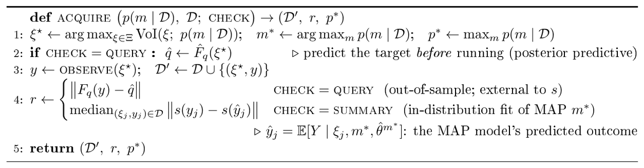
Only $\textsc{query}$ is external to the summary. The $\textsc{summary}$ residual is out-of-sample in the data (on the freshly added point) but not in the lens: a learned $ s_{\phi} $ that is insufficient for the query can keep $ r^\ast $ small even when the forecast of $ F_q $ is poor, so the LLM/SMC search can collude with $ s_{\phi} $ — fit the summary, miss the task — and a raw-trace (PF) residual cannot catch this either (a model may win likelihood by explaining nuisance detail rather than $ F_q $). Anchoring the trigger to $ F_q $ closes the loophole at no extra budget: because $ \xi^\star $ maximises model disagreement, $ F_q(y) $ is the hardest available out-of-sample test of the current pool, and it reuses the designed experiments' outcomes — the held-out evaluation set $ \xi\sim \mathcal{Q}$ stays untouched.

Idealised residual vs. the shipped approximation.

Algorithm 2 states the residual in its idealised form; all reported runs use $\textsc{check}=\textsc{summary}$, for which the implementation computes a robust approximation to $\lVert s(y_j)-s(\hat{y}j)\rVert$. Concretely, we use a per-component relative residual, median-reduced to resist outliers: $\operatorname{median}{(\xi_j, y_j)}\operatorname{median}k | s_k(y_j)-s_k(\hat{y}j)|/\max(| s_k(y_j)|, c_k)$ with a small per-component floor $c_k$ ($\textsc{NeuronBench}$, where $s=[, n\text{test}, , V{\min}, , V_{\mathrm{end}}]$); for $\textsc{ForceBench}$ the lens is the identity ($s=\mathrm{id}$) and the residual is the per-probe RMS on the raw trace. Crucially, in every benchmark we run the summary contains the target ($s\supseteq F_q$: identity for $\textsc{ForceBench}$ / $\textsc{ChemBench}$, and $n_\text{test}$ is the first component of $s$ for $\textsc{NeuronBench}$), so the $\textsc{summary}$ residual already exercises $F_q$ and the $\textsc{query}$ check would fire on essentially the same signal — which is why we did not need to re-run under $\textsc{query}$. The $\textsc{query}$ variant becomes the operative safeguard only when $s$ is lossy for the target (e.g. a learned $s_{\phi}$ that drops target-relevant structure), the regime the collusion argument above is about.

SMC for computing posterior over models.

Algorithm 3 computes posterior over LLM-proposed structures : $p(m| \mathcal{D}{0:b}) \approx \sum{i=1}^{N_m} w_i \mathbb{1}[m=m_i]$, where $w_i = p(m_i| \mathcal{D}_{0:b})$.

def $model-posterior$ $(\mathcal{D}, C; R_m, N_m, N_{\mathrm{new}},\ \textsc{loglik})\to \big(p(m\mid \mathcal{D}),\ \hat{p}(\mathcal{D})\big)$
propose $N_m$ structures $\{m_i\}_{i=1}^{N_m}$
from the LLM given $C$ (or enumerate the space)
$(\cdot,\ \log \hat{Z}_i) \gets \textsc{param-posterior}(\mathcal{D}, m_i;\ \textsc{loglik})$
for each $i$ // evidence $\log\hat{p}(\mathcal{D}\mid m_i)$; $loglik$ threaded through unchanged
$p(m_i\mid \mathcal{D}) \gets \mathrm{softmax}_i(\log\hat{Z}_i)$ // uniform structure prior
for $r = 1 \dots R_m$ // sequential refinement do
  $\rho_j \gets \textsc{residuals}(m_j, \mathcal{D})$ for *every* pooled structure $m_j$ // fit report over *all* prior attempts
  $\{m'_l\}_{l=1}^{N_{\mathrm{new}}} \sim q\big(m \,\big|\, \{(m_j,\rho_j)\}_{j=1}^{|\mathrm{pool}|},\, C,\, \mathcal{D}\big)$
  from the LLM
  // {propose a *batch* of $N_{\mathrm{new}} {\ll}N_m$
  *new* structures jointly}
  add $\{m'_l\}$ to the pool; re-score (lines 2--3);
  evidence-prune the pool back to $N_m$
end for
return $p(m\mid \mathcal{D})=\{(p(m_i\mid \mathcal{D}), m_i)\}$, $\hat{p}(\mathcal{D})=\sum_i p(m_i)\,\hat{Z}_i$

Adaptive tempered SMC for computing posterior over parameters, and evidence.

Algorithm 4 uses per-structure adaptive-tempered SMC to compute the posterior over the parameters for each model: $p(\theta|m, \mathcal{D}{0:b}) \approx \sum{i=1}^{N_p} W_i \mathbb{1}[\theta=\theta_i]$, and the evidence $Z_m=p(\mathcal{D}_{0:b}|m)$

def $param-posterior$ $(\mathcal{D}, m;\ \textsc{loglik})\to(\{\theta_i\},\{W_i\},\log Z_m)$
sample $\theta_i \sim p(\cdot\mid m)$ for $i=1.. N_p$; $W_i \gets 1/N_p$; $\lambda \gets 0$; $\log Z_m \gets 0$
$\ell_i \gets \textsc{loglik}(\mathcal{D}, m,\theta_i)$ // a plug-in: $loglik-det$ / $-pf$ / $-synth$ (Alg. Algorithm 6,Algorithm 5,Algorithm 7)
while $\lambda < 1$ // $\le J_p$ annealing rungs do
  pick $\Delta\lambda \in (0,\,1-\lambda]$ by bisection so that $\mathrm{ESS}\big(\{W_i\,e^{\Delta\lambda\,\ell_i}\}\big) = \eta N_p$
  $\log Z_m \mathrel{+}= \log \sum_i W_i\,e^{\Delta\lambda\,\ell_i}$ // evidence increment
  $W_i \gets W_i\,e^{\Delta\lambda\,\ell_i} \big/ \textstyle\sum_j W_j\,e^{\Delta\lambda\,\ell_j}$; $\lambda \mathrel{+}= \Delta\lambda$
  resample $\{\theta_i\} \propto \{W_i\}$; $W_i \gets 1/N_p$
  for $r = 1 \dots R_p$ // random-walk Metropolis at temperature $\lambda$ do
    propose $\theta_i' \sim q(\cdot\mid\theta_i)$; $\ell_i' \gets \textsc{loglik}(\mathcal{D}, m,\theta_i')$; set $(\theta_i,\ell_i)\!\gets\!(\theta_i',\ell_i')$ w.p. $\min\{1, e^{\lambda(\ell_i'-\ell_i)}\}$
  end for
end while

def $loglik-pf$ $(\mathcal{D}, m, \theta)\to\log\hat\ell$
$z_0^j \gets z_0$ for $j=1\dots N_z$; $\log\hat\ell \gets 0$
for each observation $t = 1 \dots T$ do
  $z_t^j \sim p\big(z_t\mid z_{t-1}^j,\theta\big)\quad \forall j$ // sample the stochastic transition (Euler--Maruyama; no density needed)
  $w_t^j \gets \mathcal N\big(y_t;\, g(z_t^j),\, \sigma\big)\quad \forall j$ // emission on the *observed* coordinate $g(z_t){=}V_t$; $\sigma$ fixed, no $\theta$
  $\log\hat\ell \mathrel{+}= \log\big(\tfrac1N_z\textstyle\sum_j w_t^j\big)$ // incremental log marginal (running sum over $t$)
  resample $\{z_t^j\}\propto\{w_t^j\}$
end for
return $\log\hat\ell$

The three likelihoods, and a common signature.

Algorithm 4 treats its $\textsc{loglik}$ as a black box with the signature $\textsc{loglik}(\mathcal{D}, m, \theta)\to \log\ell$; the agent plugs in one of three implementations depending on the dynamics and the compute budget: the particle filter $\textsc{loglik-pf}$ (Algorithm 5) for stochastic latents, which computes $p(\mathcal{D}|m, \theta)$ using $\hat{p}(y_{1:T}\mid m, \theta)= \prod_t \big(\tfrac1{N_z}\sum_i w_t^{(i)}\big)$, where $w_t^i$ is the weight of particle $i$; the closed-form $\textsc{loglik-det}$ (Algorithm 6) for deterministic latents, using Equation 4; or the simulation-based $\textsc{loglik-synth}$ (Algorithm 7), a cheap surrogate for the filter that fits a Gaussian to a summary statistic $s(y)$, as in Equation 11. The summary may be hand-crafted or a learned encoder $s_{\phi}$ trained once by $\textsc{train-sphi}$ (Algorithm 8); binding $s{=}s_{\phi}$ makes $\textsc{loglik-synth}$ match the common signature. The observation-model auto-selection of Equation 12 is exactly the choice among these.

def $loglik-det$ $(\mathcal{D}, m, \theta)\to\log\ell$
$z_t \gets m^t(z_0;\theta)$ for $t=1\dots T$ // one deterministic rollout (the forward model iterated $t$ times)
return $\sum_{t=1}^{T} \log \mathcal{N}\big(y_t;\ g(z_t),\ \sigma\big)$ // Equation 4

def $loglik-synth$ $(\mathcal{D}, m, \theta;\ s)\to\log\hat\ell$
simulate $y^{(r)}\sim p(\cdot\mid m,\theta)$ for $r=1\dots R$ // $R$ i.i.d. rollouts of the candidate
$\mu \gets \tfrac1R\textstyle\sum_r s\big(y^{(r)}\big)$; $\Sigma \gets \widehat{\mathrm{Cov}}_r\big[s(y^{(r)})\big] + \varepsilon I$ // summary mean \& covariance
return $\log \mathcal{N}\big(s(\mathcal{D})\ \big|\ \mu,\ \Sigma\big)$ // Equation 11

def $train-sphi$ $(C)\to s_{\phi}$
for $n = 1 \dots N_{\mathrm{sim}}$ do
  $m^{(n)}\!\sim\! p(m\mid C)$; $\theta^{(n)}\!\sim\! p(\theta\mid m^{(n)})$; $y^{(n)}\!\sim\! p(\cdot\mid m^{(n)},\theta^{(n)})$ // prior-predictive bank
end for
train $\phi$ to minimise $\textstyle\sum_n \mathcal L\big(\mathrm{head}(s_{\phi}(y^{(n)})),\ (m^{(n)},\theta^{(n)})\big)$ // classify $m$ / regress $\theta$; head discarded
return $s_{\phi}$ // the penultimate embedding: sufficient for the family, frozen and reused

SMC parameters and computational cost.

Algorithm 4 shows the SMC parameters used in the experiments. The two model-level knobs $N_m, R_m$ control the overall cost: each of the $R_m$ refinement rounds of Algorithm 3 re-fits every live structure (up to $N_m$) by a fresh $N_p$-particle adaptive-tempering SMC (Algorithm 4).

\begin{tabular}{@l l c c c l@}
\hline
quantity & symbol & \textsc{ForceBench} & \textsc{NeuronBench} & \textsc{ChemBench} & role \\
\hline
model particles & $N_m$ & $\le 14$ & $2$-- $5$ & $12$ & Algorithm 3: structures / round \\
model rounds & $R_m$ & $8\, (=B)$ & $1$ & adaptive & Algorithm 3: refinement rounds \\
new structures/round & $N_{\mathrm{new}}$ & $4$ & $1$ & $4$ & Algorithm 3: added per round if $R_m{>}0$ \\
parameter particles & $N_p$ & $200$ & $200$ & $100$ & Algorithm 4: per-structure SMC \\
rejuvenation moves & $R_p$ & $3$ & $3$ & $3$ & Algorithm 4: RW moves / rung \\
target ESS fraction & $\eta$ & $0.6$ & $0.5$ & $0.6$ & Algorithm 4: resample trigger \\
max tempering rungs & $J_p$ & $80$ & adaptive & $80$ & Algorithm 4: schedule cap \\
latent particles & $N_z$ & $1$ & $1/250$ & $1$
 {} & Algorithm 5: likelihood estimation \\
\hline
$\mathcal M$-open cap & $R_{\max}$ & --- & $3$ & $4$ & Algorithm 1: max exploration rounds \\
residual threshold & $\tau_r$ & --- & $0.18$ & $0.05$ & Algorithm 1: $\mathcal M$-open trigger \\
concentration thresh. & $\tau_p$ & --- & --- & $0.9$ & Algorithm 1: pool-shrink trigger \\
\hline
\end{tabular}

A.3 Algorithms for experiment design

Deriving the VoI.

We estimate the value of information for conducting experiment $\xi$, denoted $\mathrm{VoI}(\xi)$, as follows. Let $Y_\xi\in \mathbb{R}^d$ be the quantity the likelihood conditions on — the (hand-crafted or learned) summary $s(y_{1:T})$ under the synthetic likelihood, or the raw trace itself ($Y_\xi=y_{1:T}$, i.e. $s{=}\mathrm{id}$) under the deterministic / particle-filter likelihood. It need not be scalar: it can be a $6$-vector of spike features, a neural-net embedding, or a high-dimensional observation such as a video frame (or its object-location summary). Model its outcome as $Y_\xi=\mu(\xi)+\varepsilon$, with $\mu(\xi)= \mathbb{E}[Y_\xi\mid M, \mathrm{do}(\xi)]\in \mathbb{R}^d$ random over the posterior — a single deterministic forward simulation per particle, since the candidate dynamics carry no internal stochasticity (the property that made the likelihood Equation 4 exact) — and $\varepsilon\sim \mathcal{N}(0, \Sigma_\varepsilon)$ observation noise (the summary's sampling covariance, estimated from the $R$ synthetic draws in the SL case; $\sigma^2 I$ in the simplest scalar case). Conditioning on the mechanism class removes the between-class spread (within-class parameter variance is folded into the class mean $\bar\mu_m$; see the contrast below), so $Y_\xi\mid M\sim \mathcal{N}(\bar\mu_M(\xi), \Sigma_\varepsilon)$ and the marginal $Y_\xi\sim\sum_m p(m\mid \mathcal{D}), \mathcal{N}(\bar\mu_m(\xi), \Sigma_\varepsilon)$ is a Gaussian mixture with covariance $\Sigma_\varepsilon+\Sigma_\mu(\xi)$, where $\Sigma_\mu(\xi)=\operatorname{Var}{p(M\mid \mathcal{D})}[\mu(\xi)]$ is the $d\times d$ between-class covariance of the mean predictions. The conditional entropy $H[Y\xi\mid M]=\tfrac12\ln!\big((2\pi e)^d\det\Sigma_\varepsilon\big)$ is exact, but a Gaussian mixture has no closed-form differential entropy, so we approximate $H[Y_\xi]$ by the entropy of a single Gaussian of the same covariance (moment matching); the $(2\pi e)^d\det\Sigma_\varepsilon$ cancels in the difference:

$ I(M;Y_\xi\mid \mathcal{D})=H[Y_\xi]-H[Y_\xi\mid M] \approx\tfrac12\ln\det!\Big(I+\Sigma_\varepsilon^{-1}\Sigma_\mu(\xi)\Big),\tag{8} $

an upper bound on the true mutual information (a Gaussian maximises entropy at fixed covariance), monotone (in the Loewner order) in the between-class covariance $\Sigma_\mu(\xi)$; the scalar case $d{=}1, \ \Sigma_\varepsilon{=}\sigma^2$ recovers $\tfrac12\ln(1+\operatorname{Var}[\mu(\xi)]/\sigma^2)$. Because the map is monotone the design $\arg\max$ is insensitive to the Gaussian approximation; in practice we maximise the total between-class variance (the trace — the noise-whitened sum over feature dimensions, an A-optimal surrogate for the D-optimal $\ln\det$ that reduces to the scalar formula dimension-by-dimension), read off the class-evidence weights $p(m\mid \mathcal{D})=Z_m/\sum_{m'}Z_{m'}$ (Algorithm 4 returns each $\log Z_m$) and the per-class particle means $\bar\mu_m(\xi)=\sum_i W_i^{m}\mu_{m, i}(\xi)$:

$ \xi^\star_{\mathrm{VoI}} = \arg\max_{\xi\in \Xi}\ \operatorname{tr}!\big(\Sigma_\varepsilon^{-1}\Sigma_\mu(\xi)\big) = \arg\max_{\xi}\ \textstyle\sum_m p(m\mid \mathcal{D}), \big\lVert\bar\mu_m(\xi)-\bar\mu(\xi)\big\rVert^2_{\Sigma_\varepsilon^{-1}},\tag{9} $

where $\lVert v\rVert^2_{A}{=}v^\top A v$, $\mu_{m, i}(\xi)= \mathbb{E}[Y_\xi\mid m, \theta_i^{m}, \mathrm{do}(\xi)]$ and $\bar\mu(\xi)=\sum_m p(m\mid \mathcal{D}), \bar\mu_m(\xi)$. Using per-class means $\bar\mu_m$ rather than noisy draws keeps VoI genuine epistemic disagreement — Lindley's intuition ([14]) that the best experiment is the one whose outcome current beliefs least agree on.

Which observable to score. The VoI is computed on the inference observable $Y_\xi$ — the summary $s(y)$ under the synthetic likelihood, or the raw trace $y$ under the PF — so the design maximises information about $M$ through the same channel the posterior conditions on. We deliberately do not use the task functional $F_q(y)$ as the design objective: with $\dim y \ge \dim s(y) \ge \dim F_q(y)$, $F_q$ is typically very low-dimensional (often a scalar), carrying little discriminative signal, so we reserve it for the out-of-sample predictive check (Algorithm 2), where its role is validation, not acquisition. The summary $s(y)$ is the sweet spot — richer than the scalar task target, yet cheaper and less nuisance-dominated than the full trace, and well-defined even when the raw observation is extremely high-dimensional.

Contrast: the full predictive variance. An alternative acquisition keeps the within-class parameter spread instead of averaging it out. By the law of total variance the full two-level predictive variance splits into the between-class term of Equation 9 plus a within-class one:

$ \begin{aligned} \operatorname{tr}!\Big(\Sigma_\varepsilon^{-1}\operatorname{Var}{p(m, \theta\mid \mathcal{D})}!\big[, \mathbb{E}(Y\xi\mid m, \theta, \mathrm{do}(\xi)), \big]\Big) &=\underbrace{\sum_m p(m\mid \mathcal{D})\big\lVert\bar\mu_m(\xi)-\bar\mu(\xi)\big\rVert^2_{\Sigma_\varepsilon^{-1}}}{\text{between classes (mechanism disagreement)}} \nonumber\ &\quad+\underbrace{\sum_m p(m\mid \mathcal{D})\sum_i W_i^{m}\big\lVert\mu{m, i}(\xi)-\bar\mu_m(\xi)\big\rVert^2_{\Sigma_\varepsilon^{-1}}}_{\text{within class (parameter uncertainty)}}, \end{aligned}\tag{10} $

estimated empirically by the pooled particle variance $\sum_{m, i} w_{m, i}\big\lVert\mu_{m, i}(\xi)-\bar\mu(\xi)\big\rVert^2_{\Sigma_\varepsilon^{-1}}$ with $w_{m, i}!\propto! p(m\mid \mathcal{D}), W_i^{m}$. Only the between-class term is collapsed by identifying the class. The within-class term is residual parameter uncertainty, which is negligible once the per-structure posteriors have concentrated; in this case, this full variance coincides with Equation 9.

Optimising over a large design space.

When the design space is large, we can use various gradient free optimizers to pick the design. For continuous spaces a common choice is CMA-ES ([31]). For discrete spaces, we can use LLM-driven evolutionary search methods such as FunSearch ([42]).

A.4 Algorithms for SBI

Computing the likelihood of $p(s(y_{1:T})|m, \theta)$, as given in Equation 6, is in general intractable. In this section we discuss "likelihood free" inference methods, also known as "simulation-based inference" or SBI ([38]). Initially we assume the summary function is known; later we discuss how to learn it.

Synthetic likelihood.

One approach to SBI is to approximate the likelihood by a Gaussian over the summary features. The moments of this Gaussian are estimated by simulation — this is known as "Bayesian Synthetic Likelihood" ([49, 28]). More precisely, For each candidate $(m, \theta)$ we draw $R$ traces $(z^{(r)}, y^{(r)})!\sim p(z_{1:T}, y_{1:T}\mid m, \theta)$, throw away $z^r$, and compute the likelihood using

$ \begin{aligned} p\big(s (y_{1:T})\mid m, \theta\big) &= \mathcal{N}\big(s (y_{1:T})\ \big|\ \mu_{m, \theta}, , \Sigma_{m, \theta}\big) \ \mu_{m, \theta} &=\tfrac1R\textstyle\sum_{r} s(y^{(r)}) \ \Sigma_{m, \theta} &=\widehat{\mathrm{Cov}}_r!\big[s(y^{(r)})\big]+\varepsilon I, \end{aligned}\tag{11} $

with a small ridge $\varepsilon$ for conditioning.[^9]

[^9]: We can also replace the Gaussian with a neural network nornmalizing flow model, a technique called neural likelihood estimation (not to be confused with neural posterior estimation, which trains an amortized inference network to compute $p(m, \theta|y_{1:T})$: see ([50]) for discussion).

Learning the summary function.

In this section we discuss how to learn the summary function $s_{\phi}(y_{1:T})$. Unfortunately, if $s_{\phi}$ is optimised to maximise the synthetic likelihood of the observed dataset, the objective is trivially maximised by a constant $s_{\phi}$ (which carries no information about $\theta$ or $m$), or by an $s_{\phi}$ that discards exactly the parameter-relevant signal. This is acalled the "collapse" problem.

The fix is to learn $s$ to be sufficient for what we infer, on a held-out simulated set. In particular, we can use a bank of prior simulations ${(\theta_i, m_i, y^{(i)}{1:T})}$ — a held-out set the summary must generalise across, not a single dataset to overfit — and train $s{\phi}$ so that the latent can be recovered from the summary. This supervised signal both well-poses the problem and makes the constant solution impossible.

• Semi-automatic ABC / regression ([39]). Under quadratic loss the optimal summary is the posterior mean $s^\star(y)= \mathbb{E}[\theta\mid y]$; one approximates it by regressing $\theta$ on features of $y$ over the simulation bank, e.g. training a network $s_{\phi}(y)!\approx!\theta$ ([51]). (This is called Approximate Bayesian Computation or ABC.) Note that a constant $s_{\phi}$ has maximal regression error, so the objective prevents collapse by construction.
• Infomax / neural sufficient statistics ([40]). Maximise the mutual information $I!\big(s_{\phi}(y);\theta\big)$ over the simulated joint; a constant summary has zero mutual information, so it is the global minimiser of the objective, not a solution. Amortised-SBI summary networks ([41]) are trained jointly with a density estimator on $(\theta, y)$ pairs to the same end (see ([28]) for a survey).

Both learn a low-dimensional $s_{\phi}(y)$ that is predictive of (a sufficient statistic for) the latent, and the held-out bank is what supplies the anti-collapse signal.

Example: 1d CNN for summarizing neuron voltage trace.

In Appendix E.8, we give a concrete example of the regression approach, where we train a 1d CNN to map the neuron voltage trace $y_{1:T}$ to the label of the correct class (4 possible model types) and a corresponding model parameter (the max conductant $g$). The model has two output heads; the penultimate layer is a learned feature vector $s_{\phi}(y) \in \mathbb{R}^d$, which we use as the summary statistic.

Sufficiency as the hypothesis pool grows.

A learned summary is only as informative as the simulated family it was trained on, so in the $\mathcal M$-open loop sufficiency cannot be a fixed, global property — the pool the agent chooses among changes over time. Three points make it well-posed. (i) It is task-relative and re-learned. A statistic is sufficient for choosing among the current pool ${m_1, \dots, m_K}$ iff the likelihood ratios depend on $y$ only through it; a classifier trained to separate the current members' simulations has, at its optimum, exactly such a statistic (its log-odds), and adding a proposed hypothesis simply adds a class and re-fits — cheap, since the simulations are already drawn for the synthetic likelihood, and the summary dimension grows with the pool. (ii) It can be amortised. Training $s_{\phi}$ over the LLM's prior-predictive mechanism family (rather than the current pair) generalises to in-distribution proposals without re-fitting. (iii) It is checkable, with a model-agnostic anchor. A particle filter needs no summary, so it is a sufficiency-safe gold standard: when a new mechanism is proposed, disagreement between the cheap synthetic likelihood and a spot-check particle filter (or a simulation-based-calibration failure) flags an insufficient summary and triggers re-learning (Appendix F.1 validates this synthetic-likelihood/particle-filter equivalence in the stochastic- $\textsc{NeuronBench}$ setting). The approximation is therefore monitored and repairable, not assumed: a proposal whose signature lies in a data dimension $s_{\phi}$ discarded is invisible until re-learning, and the particle-filter anchor is what makes that safe. Co-training the observation abstraction with the mechanism expansion end-to-end we leave to future work.

A.5 Auto-selecting the observation model

When the latent dynamics are stochastic, the likelihood is intractable, and there is a menu of approximations trading accuracy against compute: a bootstrap particle filter on the raw observation (assumption-free but costly, Algorithm 5); a synthetic likelihood Equation (5) on a hand-crafted feature vector $s(y)$ or on a learned summary $s_{\phi}(y)$ — cheap, but only as sufficient as the summary; or, when the process noise is negligible, a single deterministic rollout Equation (4). No single choice is best for every discrimination problem, so we let the agent choose the observation model $o$ exactly as it chooses the experiment.

Observation model as a design decision.

Writing $p_o(y\mid m, \xi)$ for the likelihood under observation model $o$, the agent picks

$ \begin{aligned} o^\star &= \arg\max_{o, \in, {\mathrm{PF}, , \mathrm{feat}, , s_{\phi}}}\ \frac{\mathrm{MI}_o\big(m;\ y\mid \xi\big)}{\mathrm{cost}(o)} \ \mathrm{MI}o\big(m;y\mid \xi\big) &=H(p(m))-\mathbb{E}{p_o(y\mid \xi)}!\big[H\big(p_o(m \mid y)\big)\big], \end{aligned}\tag{12} $

Here $H(p(m))=-\sum_m w_m\log w_m$ is the entropy of the prior over models, and the posterior is given by

$ p_o(m\mid y)= \frac{w_m, p_o(y \mid m, \xi)} {\sum_{m'}w_{m'}, p_o(y \mid m', \xi)}\tag{13} $

The posterior predictive distribution over observations is given by

$ p_o(y \mid \xi)=\sum_m w_m p_o(y \mid m, \xi)\tag{14} $

We approximate the expectation in Equation 12 by Monte Carlo. To draw an observation from the posterior-predictive $p_o(y\mid \xi)=\sum_m w_m!\int p(y\mid m, \theta, \xi), q(\theta\mid m), d\theta$ we sample ancestrally: first a model $m\sim q(m)$ from the SMC model samples, then $\theta\sim q(\theta\mid m)$ from that model's SMC parameter particles, and finally an observation $y\sim p(y\mid m, \theta, \xi)$ from the forward model — the generative simulator is shared across all $o$; the observation model $o$ enters only in the scoring. For each of the $S$ sampled $y_s$ we form the posterior $p_o(m\mid y_s)$ Equation (13) and average its entropy,

$ \mathrm{MI}o ;\approx; H\big(p(m)\big) ;-; \tfrac1S\sum{s=1}^{S} H\big(p_o(m\mid y_s)\big),\tag{15} $

where each posterior needs the per-model marginal likelihood $p_o(y_s\mid m, \xi)=\int p_o(y_s\mid m, \theta), q(\theta\mid m), d\theta$, which we approximate by a plug-in at the model's MAP parameters.

Cheap approximation of the objective.

In practice, rather than evaluate the entropy in Equation 15 directly, we use a cheaper $0/1$ surrogate — a truth-free discrimination probe: on the discriminating protocol, simulate single experiments from each candidate in turn (generators weighted uniformly) and measure how often $o$ 's log-evidence gap identifies the generator, averaged over generators — never peeking at the truth.

Concretely, let $\mathcal M={m_1, \dots, m_K}$ be the current pool. We treat each candidate $m'$ in turn as a hypothetical generator, simulate $R$ experiments from it on the discriminating design $\xi$, and score each simulated dataset under every candidate's likelihood; the probe's discrimination power is the rate at which the maximum-likelihood candidate is the true generator,

$ \widehat{d}(o);=;\frac{1}{K R}\sum_{m'\in\mathcal M}\ \sum_{r=1}^{R} \mathbb{1}!\Big[\ \arg\max_{m\in\mathcal M}\ p_o\big(y^{(m', r)}\mid m, \xi\big)\ =\ m'\ \Big], \qquad y^{(m', r)}\sim p\big(y\mid m', \xi\big),\tag{16} $

where $y^{(m', r)}$ is the $r$-th experiment simulated from generator $m'$ — the true cell is never simulated or observed, hence truth-free. $\widehat{d}(o)$ ranges from $1/K$ (chance: $o$ cannot tell the candidates apart, so the $\arg\max$ is random) to $1$ (perfect separation), and the agent substitutes it for $\mathrm{MI}_o$ in Equation 12, picking $o^\star=\arg\max_o \widehat{d}(o)/\mathrm{cost}(o)$. This costs only $K^2R$ likelihood evaluations (score $KR$ simulated datasets, and $K$ candidates inside the $\arg\max$), although each likelihood evaluation itself costs $R' \approx 60$ rollouts for the feature vector, or $N_z$ particles for PF.

The probe makes two deliberate approximations to 15. (i) Hard $0/1$, not entropy. It replaces the posterior entropy $H!\big(p_o(m\mid y)\big)$ with the indicator that the MAP candidate is correct: cheaper (an $\arg\max$, with no per-sample entropy or nested $\theta$-marginal likelihoods) and it uses the same $\arg\max$ that the downstream model selection uses, but it throws away how confidently the pool is resolved. (ii) Uniform generators, not $w_m$. It draws the generator uniformly ($1/K$) rather than from the model posterior $w_m$, so it scores average-case separability rather than posterior-weighted information gain. Both approximations are what make it cheap and robust to a mis-calibrated posterior — and both are why it can be blind to a summary that confuses one specific pair while separating the rest (the failure the particle-filter spot-check, described below, is designed to catch). It is nonetheless monotone in $\mathrm{MI}_o$: a more discriminating likelihood both raises the mutual information and lowers the MAP error rate (Fano's inequality), so ranking observation models by $\widehat{d}(o)/\mathrm{cost}(o)$ tracks the cost-aware VoI of Equation 12.

Cost of each observation model.

The term $\mathrm{cost}(o)$ is the compute of one likelihood evaluation, $p(y_{1:T}| \xi, m, \theta)$. We measure it in units of the shared primitive that both cheap models and the particle filter are built from — a single forward simulation of a candidate mechanism through the protocol (an $O(T)$ Fox–Lu SDE rollout, Equation 25) — so the three observation models differ only in how many rollouts they consume per candidate per experiment:

• Feature synthetic likelihood (the unit): draw $R$ rollouts, reduce each to the feature vector $s(y)$, and fit/score a Gaussian, so $\mathrm{cost}(\mathrm{feat})\propto R$ (we use $R{=}60$).
• Learned summary $s_{\phi}$: the same $R$ rollouts plus a forward pass through the frozen encoder (negligible), with the one-time family pre-training amortised over the whole run — so $\mathrm{cost}(s_{\phi})\approx\mathrm{cost}(\mathrm{feat})$ (with $R{=}80$, a factor ${\approx}1.3$).
• Particle filter: propagate $N_z$ latent trajectories through all $T$ steps with resampling, so $\mathrm{cost}(\mathrm{PF})\propto N_z$ and $\mathrm{cost}(\mathrm{PF})/\mathrm{cost}(\mathrm{feat})\approx N_z/R$.

Concretely we take $\big(\mathrm{cost}(\mathrm{feat}), , \mathrm{cost}(s_{\phi}), , \mathrm{cost}(\mathrm{PF})\big) =(1, , 1.3, , 7)$; the $\times 7$ is the $N_z/R$ ratio at our settings. (The one-time $s_{\phi}$ training and the per-refit are charged separately, not to a single evaluation — they are amortised because $s_{\phi}$ is frozen across all worlds, protocols, and pools.) This is design over the observation model, not the experiment — so the agent defaults to the cheap summary and pays for the filter only where its discrimination clearly justifies the compute.

The particle-filter spot-check.

The discrimination probe averages over generators, so it scores whether $o$ separates the pool on average; it cannot see a cheap summary's specific blind spot. A learned $s_{\phi}$ trained on the mechanism family may confuse a single pair whose signatures collapse in its low-dimensional embedding while discriminating all the rest well — giving a deceptively high pooled score yet a confidently wrong answer on the world where that pair is the question. We therefore make the particle-filter anchor operational as a spot-check: whenever a cheap model $o\neq\mathrm{PF}$ is selected, we re-score the collected data with both $o$ and the particle filter (over the top few candidates by posterior) and compare their MAP models; on disagreement we fall back to the PF. The cheap summary is thus used only where it is verifiably sufficient — it agrees with the assumption-free filter — and the PF catches the rest. This is the safeguard that makes a fast, possibly-insufficient summary safe to deploy inside the $\mathcal{M}$-open loop (Algorithm 3): the observation model, like the experiment, becomes something the agent chooses and verifies from data rather than a hand-set knob. Appendix F instantiates both — the cost-aware choice and the spot-check — on the electrophysiology benchmark, and reports how often each observation model is chosen and how often the spot-check overrides a cheap choice.

B. Experimental results: further details

\begin{tabular}{@l l p{1.85cm} p{2.35cm} p{2.75cm} l@}
\hline
Benchmark & Domain & Model class & Observation space & Design space & Ref. \\
\hline
\textsc{ForceBench} & Physics & ODE (force law) & 2D trajectory (time series) & $\mathbb{R}^2\times$ discrete (13-menu) & ([1]) \\
\textsc{ChemBench} & Chemistry & algebraic rate law (sym. reg.)& single scalar (initial rate) & $\mathbb{R}^7$ (continuous) & ([2]) \\
\textsc{NeuronBench} & Neuroscience & ODE (Hodgkin--Huxley) & 1D voltage trace (time series) & input current $\times$ channel blocks & ours \\
\textsc{NeuronBenchStoch} & Neuroscience & SDE (stochastic Hodgkin--Huxley) & 1D voltage trace (time series) & input current $\times$ channel blocks & ours \\
\hline
\end{tabular}

The datasets we use are listed in Table 3. We evaluate the forecasts for each agent $\alpha$ after $k$ experiments as follows. For $\textsc{ForceBench}$ we first compute $\mu_{i, t, b}(\alpha) = E[Y^i_{t}| \xi^i, \mathcal{D}_{0:b}, \alpha]$ for each time step $t$ of each test trajectory $i$, and then compute the mean squared error (MSE):

$ \text{MSE}b(\alpha) = \frac{1}{N{\text{test}}} \sum_{i=1}^{N_{\text{test}}} \frac{1}{T} \sum_{t=1}^T (\mu_{i, t, b}(\alpha) - \mu^*_{i, t, b})^2 $

where $\mu^*_{i, t, b}$ is the (noise free) expectation under the ground truth model. For $\textsc{NeuronBench}$ we use $\mu_{i, j, b}(\alpha) = E[s_j(Y^i_{1:T})| \xi^i, \mathcal{D}_{0:b}, \alpha]$ for each summary feature $j$, and compute the MSE by averaging over features instead of time steps. We then plot MSE vs $b$, for $b=1: B$, where $B=8$ is the maximum number of experiments. We also plot MSE for $k=0$, which is the performance just given $\mathcal{D}_0$, before any experiments are performed.

C. Physics: further details

C.1 Details on the benchmark

\begin{tabular}{@c l l p{0.44\textwidth}@}
\hline
# & world & pairwise force magnitude $F(r, t)$ & Comments \\
\hline
\multicolumn{4}{@l}{\emph{Two-particle, central, radial (single fixed source at the origin)}}\\
1 & \textsc{gravity} & $k\, q_iq_j/r$
 {} & Simple attractive force\\
 2 & \textsc{yukawa} & $k\, q_iq_j\, K_1(r/\lambda)/\lambda,  \lambda{=}2$
  {} & Screened (2D Helmholtz) kernel: $\sim\!1/r$ at short range, exponentially suppressed beyond $\lambda$ \\
 3 & \textsc{coulomb} & $k\, q_iq_j/r^{2}$ &
 Simple attractive force \\
 4 & \textsc{oscillator} & $k\, q_iq_j\cos(\omega t{+}\phi)/r$
  {} & Time-varying coupling that periodically reverses sign \\
 5 & \textsc{fractional} & $k\, q_iq_j/r^{\, 3-2\alpha},  \alpha{=}\tfrac12\, ({\equiv}1/r^2)$
  {} & Fractional Laplacian $-(-\nabla^2)^{\alpha}$ with $\alpha=\tfrac12$ \\
 6 & \textsc{extra-dim} & $k\, q_iq_j\, \Phi_{\mathrm{KK}}(r)$ &
 $1/r^2$ (short range) to $1/r$ (long range) transition,
 defined by the Kaluza--Klein image-sum kernel \\
\hline
\multicolumn{4}{@l}{Non-radial or many-body (superposed background, or $N$ mutually-interacting bodies)}\\
7 & \textsc{circle} & $k\, q_iq_j/r^{\, 3-2\alpha},  \alpha{=}\tfrac34$
 {} & Fractional Laplacian with ring of particles \\
8 & \textsc{ether} & $k\, q_iq_j/r$ 
 {} & Central law + global drift, $a_i=-F\, \hat{r}/m_i+\alpha\, \hat {\mathbf{y}}$ \\
9 & \textsc{hubble} & $k\, q_iq_j/r$
 {} & Central law + position dependent Hubble flow,
$a_i=-F\, \hat{r}/m_i+H(\mathbf{r}_i)$ \\
10 & \textsc{dark-matter} & $k\, q_iq_j/r,  q_j{\in}\{1, \underline{5}\}$
 {} & Hidden number of other particles \\
11 & \textsc{three-species}& $k\, q_iq_j/r,  q_j{\in}\{\underline{1, 3, -2}\}$
 {} & 3 hidden classes (one repulsive) + 5 neutral probes\\
\hline
\end{tabular}

$\textsc{ForceBench}$ (which is just a wrapper on $\textsc{DiscoverPhysics}$ from ([1])) requires an agent to infer the unknown force law governing the behavior of two or more particles in a 2d space. Each particle $i$ has an associated kinematic state: position $\mathbf{r}_i$, velocity $\mathbf{v}_i$, and a "generalized charge" $\mathbf{q}_i=(s_i, c_i)$, where $s_i$ is the source charge, controlling how strongly particle $i$ generates the field, and a response charge $c_i$ controlling how strongly it feels the field generated by others. When $s_i=c_i$ for all particles, this reduces to a standard symmetric pairwise interaction. In this case, $q_i$ might represent a charge (for electric fields) or a mass (for gravitational fields). The pairwise force takes the general form

$ \mathbf{F}{i \leftarrow j} = F{\text{mag}}(r_{ij}, \mathbf{q}_i, \mathbf{q}j, t) \hat{\mathbf{r}}{ij} $

where $r_{ij}= || \mathbf{r}_i-\mathbf{r}j||$ is the distance between the particles, and $\hat{\mathbf{r}}{ij}$ is the unit separation vector from source to receiver (so $-\hat{\mathbf{r}}$ is attractive).

There are 11 different laws or worlds, shown in Table 4. We group them into 6 two-particle worlds, which follow a radial force centered on particle 1, and 5 "extra" worlds, which have slightly different semantics, as listed in the table.

From Newton's second law, $\mathbf{F} = m \mathbf{a}$, we can derive the acceleration $\mathbf{a}=(a_x, a_y)$ of a particle as follows:

$ \mathbf{a} = - F_{\text{mag}} \hat{\mathbf{r}} / m\tag{17} $

If there are multiple particles, we sum the forces:

$ \mathbf{a}i = -\sum{j \neq i} F_{ij} \hat{\mathbf{r}}_{ij} / m_i $

From this, we can derive the velocity by integration, and hence generate the trajectory of each particle from its initial conditions.

The benchmark requires the agent to submit a Python function that returns the predicted trajectory. The function must satisfy the following signature:

def discovered_law(pos1, pos2, p1, p2, velocity2, duration, **params):
 ...
 return trajectory

Here params are free parameters of the law which can be fit to the collected data by the $\textsc{ForceBench}$ environment before it calls the above function. The agent can choose the initial position of particles 1 and 2, and the velocity of particle 2. (The velocity of particle 1 is fixed at $(0, 0)$.) The meaning of the control knobs $p_1$ and $p_2$ varies across the worlds: sometimes they represent masses, sometimes charges (see Table 4 for details).

The LLM baseline method from ([1]) uses an LLM to generate code which computes the acceleration function $\mathbf{a}$, from which it derives the trajectory by integration. In Table 8, we give examples of the generated code. In MDA, we instead estimate $F_{\text{mag}}$, and then derive $\mathbf{a}$ using Newton's law in Equation 17, which we pass to the integrator. (MDA also estimates its own parameters, using the posterior mean associated with the submitted model, rather than using the environment's fitting function.) We could of course ask the LLM to generate $F_{\text{mag}}$ instead, but this would be a different method to the one used in ([1]).

C.2 The design space

An experiment (action $a$) is a single probe launch in the benchmark's own API: the probe is released from position $(r_0, 0)$ with velocity $v$, under two scalar coupling knobs $(p_1, p_2)$ whose roles (source charge, probe inertia, …) are part of what must be discovered.

The design space $\Xi$ for $\textsc{TwoParticleWorlds}$ is the fixed menu of $13$ such launches in Table 5. This space was chosen by an LLM to cover the relevant dimensions. The design space for $\textsc{MultiParticleWorlds}$ is shown in Table 6. VoI (and the LLM/random acquisition baselines) selects one action per round. Note that these are discrete spaces, to make the VoI maximization problem simple.

\begin{tabular}{@c c c c c l@}
\hline
action $a$ & $r_0$ & $v$ (launch) & $p_1$ & $p_2$ & purpose \\
\hline
$1$-- $8$ & $\{1.5, 2, 3, 4, 5, 6, 8, 10\}$ & $[0, 0]$ (radial drop) & $1$ & $1$ & radial profile (short $\to$ long $r_0$) \\
$9$-- $10$ & $\{2, 4\}$ & $[0, 0.4]$ (tangential) & $1$ & $1$ & orbit shape (angular momentum) \\
$11$ & $4$ & $[0, 0]$ & $2$ & $1$ & identify the role of $p_1$ \\
$12$ & $3$ & $[0, 0]$ & $1$ & $2$ & identify the role of $p_2$ \\
$13$ & $4$ & $[0, 0]$ & $2$ & $2$ & vary both knobs \\
\hline
\end{tabular}

\begin{tabular}{@l l l c l@}
\hline
world & system & each experiment sets & # & discovers \\
\hline
ether & central $+$ drift $\vec{a}{=}(0, \alpha)$ & $5$ orbiters, $r{\in}[3, 8]$, $v{=}2.8$ & $6$ & $F$, $\alpha$ \\
Hubble & central $+ H\vec{r}$ & $5$ orbiters, $r{\le}8$ & $6$ & $F$, $H$ \\
circle & $11$-body ring & ring $R$, launch $v$, $R$-scaled $t$ & $6$ & exponent $p$ \\
dark-matter & $+\, K$ hidden masses & continuous $(x, y, v_x, v_y)$ & $\infty$ & #\, \&\, loc. of masses \\
three-species & $30$ bg., hidden couplings & probe \emph{direction} & $4$ & couplings\, $\to$ \, species \\
\hline
\end{tabular}

C.3 Interactive app

To make the task concrete, we built PhysicsPlayground, a self-contained web app that lets a reader play a simplified version of the game that the agent must solve. Figure 7 shows a screenshot. The top row is a transduction puzzle in the style of ARC-AGI but for a physical law: two training experiments (a launch radius $r_0$ and the resulting orbit $r(t)$, the raw trajectory the discovery algorithm fits) and two test forecasts — a launch at a new radius, and a launch under a perturbed source ($\mathrm{do}(\text{mass}{\times}2)$), the interventional "what if" the method targets. At the bottom of the screen is the playground, where the user can launch their own orbits, read the animated trajectories, and work out the force law. Finally they submit their forecast for each test launch in the top right, and they can then choose to reveal the truth to self-score.

C.4 Parameters and their priors

On $\textsc{ForceBench}$ the candidate structures are open ended: the LLM proposes a force magnitude $F(r, q_i, q_j, t;\theta)$, where each model has its own free parameters and bounds. Each free parameter takes a uniform prior over the proposer-declared bounds; see Table 7. The joint prior factorises as

$ p(m, \theta)=p(m), \prod_{k=1}^{C_m}p_k(\theta_k) $

where we use a structure prior of the form

$ p(m)\propto e^{-\lambda C_m} $

where $C_m$ is the number of free parameters of structure $m$, and $\lambda=2.5$ is the Occam penalty per free parameter. Thus the posterior over structures is

$ \begin{aligned} p(m\mid \mathcal{D}) &\propto Z_m, e^{-\lambda C_m} \ Z_m &=\int p(\mathcal{D}\mid\theta, m), p(\theta\mid m), d\theta \end{aligned} $

where $Z_m$ is the SMC marginal likelihood. The explicit $e^{-\lambda C_m}$ term is added as an additional regularizer, since on near-deterministic data ($\sigma{=}0.03$), a more flexible form can win $Z_m$ by fitting the observation noise. (Note that penalizing the length of the representation of the function $F$ — computed either by string length or Halstead complexity ([52]) — did not work as well, since that ignores the flexibility of the underlying "elementary" functions that are used.)

We currently fix the observation noise to $\sigma=0.03$. However, this could invite overfitting, since a more flexible model can win marginal evidence by driving residuals below that noise floor. The principled remedy is to be Bayesian about $\sigma$ — put an inverse-gamma prior on the residual variance and marginalize it, giving a Student-t marginal likelihood $-(a+M/2)\log!\big(b+\tfrac12\mathrm{SSE}(\theta)\big)$ over all $M$ residuals, whose scale is tied to the known noise floor via $b$. This removes the arbitrary fixed- $\sigma$ dependence and, being scale-invariant in the residuals, no longer rewards fitting below a floor.

Empirically, however, $\sigma$-marginalization alone does not cure the overfitting, and can worsen model selection: with the hundreds of residuals these many-body worlds provide, the marginal likelihood over-rewards any reduction in SSE by a factor $\sim!M/2$ (a Lindley-paradox-like effect), so a flexible form that absorbs the observation noise wins, and the Occam factor alone does not compensate. Fortunately the explicit prior on models, $p(m)$, to encourage simplicity suffices. This combination is robust and, on Hubble, converts a near-miss (the pool's spurious time-modulated $1/r$, a small $\varepsilon$ fitting the noise) into the clean $1/r$ result reported above.

\begin{tabular}{@l l l l@}
\hline
Quantity & Symbol & Prior / value & Role \\
\hline
\multicolumn{4}{@l}{Inferred: a candidate's free coefficients $\theta$ (prior $=$ Uniform over the declared bounds):}\\
coupling strength & $k$ & $\mathrm{Uniform}(0.01, \, 5)$ & force magnitude \\
screening length & $\lambda$ & $\mathrm{Uniform}(0.5, \, 40)$ & Yukawa / range cutoff \\
radial exponent & $p$ & $\mathrm{Uniform}(0.5, \, 2.5)$ & power-law falloff $1/r^{p}$ \\
oscillation frequency & $\omega$ & $\mathrm{Uniform}(0.1, \, 6)$ & time-varying force \\
oscillation phase & $\phi$ & $\mathrm{Uniform}(0, \, 2\pi)$ & time-varying force \\
\hline
\multicolumn{4}{@l}{\emph{Structure prior (Bayesian Occam over the parameter count):}}\\
number of free params & $C_m$ & $p(m)\propto e^{-2.5\, C_m}$ & penalise flexibility \\
\hline
\multicolumn{4}{@l}{\emph{Fixed (not inferred):}}\\
charge / inertia roles & $q_i, q_j, m$ & $q_i{=}1$; $p_1, p_2$ set charge, inertia & driving force \\
integrator step & $\Delta t$ & $0.005$ (symplectic) & forward model \\
measurement times & $t$ & $\{0.5, 1, 1.5, 2, 3, 4\}$ & readout grid \\
seed launch & $\mathcal{D}_0$ & one passive drop at $r_0{=}3$ & warm-start data \\
position noise & $\sigma$ & $0.03$ (fixed Gaussian) & likelihood 
\end{tabular}

C.5 Laws discovered for TwoParticleWorlds

::: {caption="Table 8: Laws discovered for the six ForceBench worlds by MDA and the pure LLM agent (Opus 4.7, B=8 experiments; regenerated from the same runs as Figure 2). For each world we show the true force law and each method's best (lowest-error) submitted law with its fitted parameters (MDA submits a force magnitude F; the LLM writes an acceleration line, of which we show $a_x$ or the radial a, whichever is simpler). nMSE is the DiscoverPhysics normalized MSE (MSE / test-trajectory variance), geometric mean over the 9 runs. %pass_<0.1 is the fraction of runs with nMSE below the paper's 0.1 threshold (dropping their explanation score); % $\equiv$is the fraction exactly form-equivalent to the true law (form-MSE <1$0^-3$ at unit charges, isolating the form from the charge-role)."}

:::

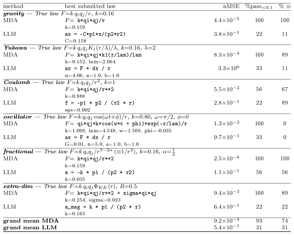
Table 8 shows the laws discovered by MDA and the pure LLM agent after $B=8$ experiments on $\textsc{TwoParticleWorlds}$. Looking at the details of the discovered laws, we see that sometimes the result looks different from the truth but is mathematically equal. For example, on $\textsc{fractional}$ the truth is $F = k q_i q_j / r^{3-2 \alpha}$ with $\alpha=0.5$, and MDA proposes the simpler but equivalent expression $F = k q_i q_j / r^{2}$.

We score each run two ways. The exact-form rate (% $\equiv$) is the fraction of runs whose submitted law is functionally equivalent to the truth after removing parameters and constants; we judge this by the form-MSE at unit charges ($p_1{=}p_2{=}1$), which isolates the radial/temporal form from the charge-role handling, and call a run exact when this form-MSE is below $10^{-3}$. The numeric rate (%pass$_{<0.1}$) instead uses the DiscoverPhysics benchmark's own criterion: the normalized MSE, nMSE $=$ MSE $/\mathrm{Var}$ where $\mathrm{Var}$ is the variance of the held-out test trajectories (accounting for the different total particle travel across worlds), counting a run as passing when nMSE

lt;0.1$. We drop the benchmark's second gate — an LLM-judged explanation score $\ge0.9$ — because we found it unreliable (Appendix C.7).

Under these metrics MDA recovers the exact form in $74%$ of runs and passes numerically in $93%$, versus $31%$ and $31%$ for the LLM agent budget-matched to one experiment per round (the same $B=8$ budget MDA uses). This gap is one of data efficiency, not capability. The DiscoverPhysics benchmark lets an agent submit a batch of experiments each round, so its nominal $16$-round budget collects far more than $16$ experiments; run un-throttled in its native batched protocol, our LLM agent uses ${\sim}41$ experiments and reaches nMSE $0.013$, essentially reproducing the paper's strongest agent (Opus, nMSE $0.01$; ([1])). MDA reaches that same accuracy with only $8$ one-per-round experiments — a ${\sim}5\times$ data-efficiency advantage (Figure 2, right).

Is the advantage the curated design menu?

MDA chooses experiments from the fixed $13$-launch menu of Table 5, hand-built to contain informative probes, whereas the pure agent chooses initial conditions freely. One might worry that this curated design space — rather than the Bayesian inference — is what drives MDA's lead. To test this we ran an Opus agent given the same menu: each round it picks a menu experiment, and after $8$ experiments it submits its own best-fit force law (no SMC). It reaches only $22%$ numeric pass and $17%$ exact-form — no better than the free-choice Opus agent ($31%$), and far below MDA's $93%$. So the menu is not the source of MDA's advantage: handed the identical design space, an LLM's own propose-and-fit inference remains far weaker than MDA's SMC-evidence selection and VoI design. (Conversely, the base-model sweep of Appendix C.8 shows the gap does narrow with a much stronger agent, Fable 5 — so the advantage is the inference, and its size depends on how good the free-form agent's own inference is.)

C.6 Data efficiency curves

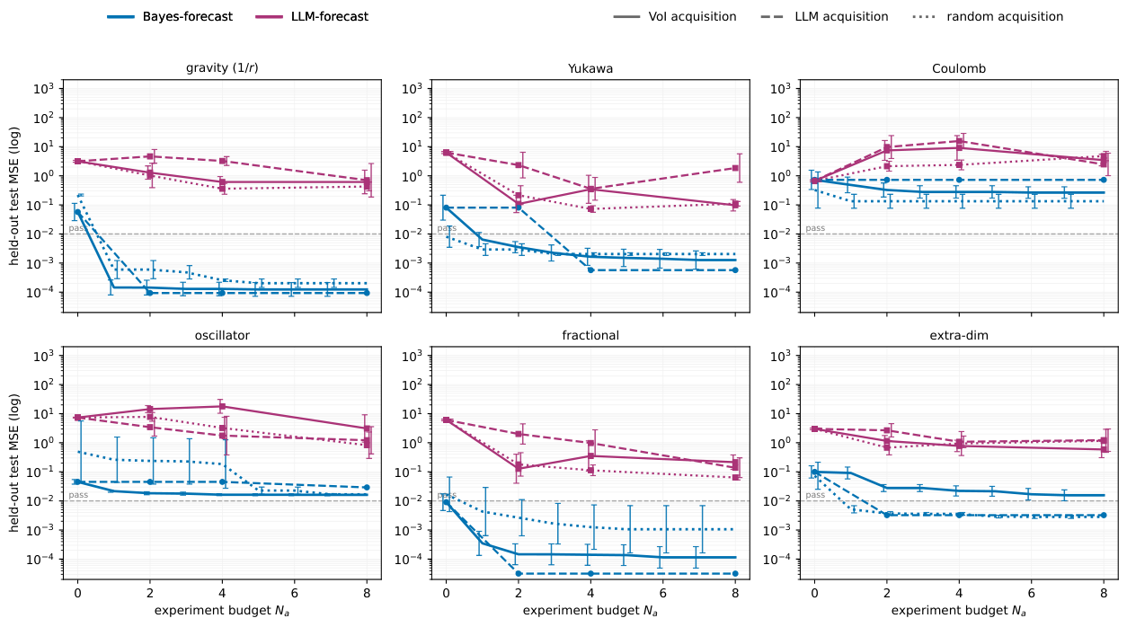
In Figure 8 we plot the data efficiency curves for each of the six $\textsc{TwoParticleWorlds}$, from which the aggregated results in Figure 2 are obtained. In Figure 9 we plot similar curves for each of the five $\textsc{MultiParticleWorlds}$. We see that MDA beats LLM agent by a large margin.

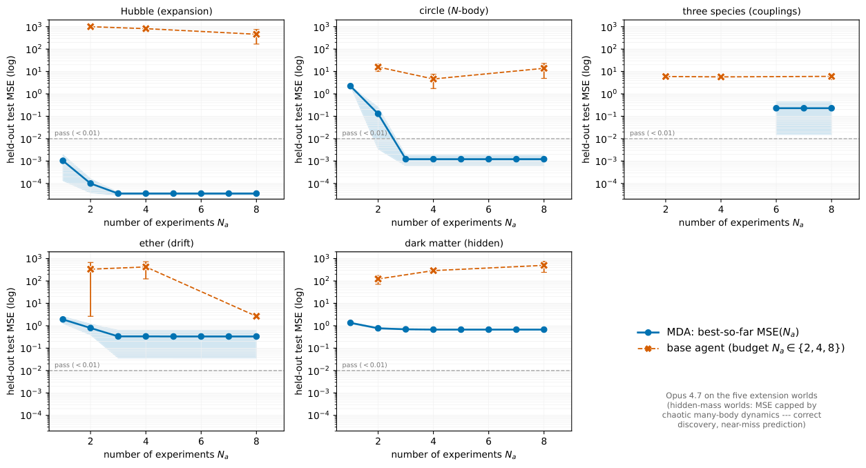
The above figures, and Figure 2 in the main text, follows the DiscoverPhysics protocol and reports only the numeric metric. Figure 10 adds the symbolic (exact-form) view we use as a secondary, more stringent check: the fraction of runs whose submitted force law is the ground-truth form exactly (form-MSE

lt;10^{-3}$ on held-out unit-charge cases, isolating the functional form from the charge-role). MDA recovers the exact form for ${\sim}70%$ of runs within a few experiments, roughly twice the Opus agent's rate; note this exact-form test is stricter than, and can diverge from, numeric accuracy (a strong agent may write a law it cannot accurately integrate, and a predictive law need not be the canonical form) — see Appendix C.8 for the Fable comparison, where the gap between the two metrics is largest.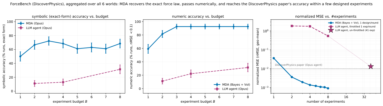

lt;0.1$): MDA reaches ${\sim}93\%$; the agent ${\sim}31\%$. *(right)* nMSE vs. number of experiments, with the un-throttled Opus agent (star) reproducing the DiscoverPhysics paper's ${\sim}0.01$ at its native ${\sim}41$-experiment budget. Error bars are $\pm1$ SE over the $6{\times}9$ runs.">

C.7 Explanation metric

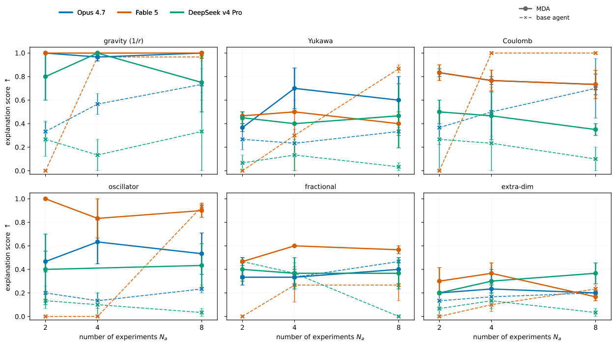
A low held-out MSE does not certify a correct model: a law can be "right for the wrong reasons, " fitting observed orbits without capturing the mechanism. ([1]) proposed to fix this by asking each agent to return a text explanation to accompany its predicted law; this is then evaluated using an LLM judge. However, we have found this metric to be unreliable. For example Figure 11 shows that the explanation score is essentially flat in the number of experiments, and often moves non-monotonically (more data making it worse), because the discovered functional form converges within the first couple of experiments and the residual movement is run-to-run variation in how the LLM phrases the same law, filtered through an $11$-level judge.

An alternative is to test the ability of the model to predict under different kinds of novel distribution shifts, which is equivalent to testing its robustness to interventions on the mechanism. As proved in ([4]), an agent that can perform such out-of-distribution predictions reliably must have learned a causally correct model of the world. In fact $\textsc{ForceBench}$ already evaluates models performance in this way: it measures MSE on test sets that combine one long-horizon probe and two single-knob interventions. Focusing on predictive performance on interventional test sets is not only more robust, but it also more general, since it does not require comparing to some (usually unknown) "true model".

C.8 Robustness to the base model

The headline comparison uses Opus 4.7 as the shared base model, where the pure LLM agent is weak (Table 8). This raises a fair question: is MDA's advantage an artifact of a particular (weak) agent, and would it vanish with a stronger base model? In this section, we consider three base models spanning a wide capability range: Opus 4.7, Fable 5, and DeepSeek v4.

Figure 12 shows the MSE results across the 6 worlds. We see that Fable is able to catch up with MDA's data efficiency in 5 out of 6 of the worlds. However, we note that we beat Fable at small number of experiments using a much cheaper model (DeepSeek), provided we augment it with MDA (which has negligible cost). Further experimentation with Fable on $\textsc{MultiParticleWorlds}$ and other scientific domains is left to future work (since running Fable is expensive).

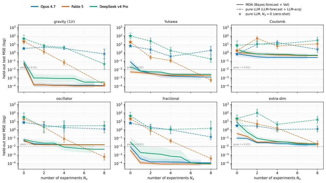
In Figure 13 we aggregate results across worlds, but also show symbolic accuracy, not just MSE. Two patterns emerge. First, MDA is essentially model-agnostic: its numeric pass rate is $89$ – $94%$ and its exact-form rate $74$ – $83%$ regardless of the base model — the Bayesian machinery (SMC evidence, VoI design) does the heavy lifting, and a stronger proposer helps only at the margin. Second, the pure agent is highly base-model-dependent: its numeric pass rate swings from $26%$ (DeepSeek) and $31%$ (Opus) up to $81%$ for Fable 5, a much stronger recent model. So the striking gap against the Opus agent narrows sharply against Fable.

Even against the strongest agent we tested, MDA's extra inference on the same proposals never hurts and sharply helps: MDA attains the higher numeric pass rate ($94%$ vs. $81%$; Figure 13, middle) and reaches $\text{nMSE}\approx10^{-3}$ in $\sim!2$ designed experiments, an accuracy the Fable agent reaches only at $B{=}8$ (right). On the joint metric that credits a run only when it is both exact-form and numerically correct, the two methods tie ($74%$ each). The one axis on which the Fable agent leads is pure exact-form recovery ($93%$ vs.\ $78%$), and that lead is partly illusory: a free-form agent writes its own integrator, so it can name the exact law without being able to compute with it. On coulomb, for instance, the Fable agent scores $100%$ exact-form but only $11%$ numeric, whereas MDA — using the same proposals with a vetted forward model — scores $67%$ numeric.

The residual exact-form gap is not because MDA cannot propose the exact law: it uses the same LLM proposer (Fable), and a truth-equivalent form is present in its $N_m{\approx}14$-candidate pool in the large majority of runs. It is a model-selection effect: the Bayesian evidence sometimes outvotes the truth in favour of a slightly more flexible form that fits the observation noise marginally better (e.g. a spurious weak time-modulation on top of the correct radial law). We counter this with a parsimony submission rule: at submission, among the pool forms that share the winning force-profile shape $F(r)$, we return the fewest-parameter member — evicting the over-elaborated near-duplicates the $\mathcal{M}$-open exploration introduces, the same ESS-eviction idea used in $\textsc{ChemBench}$ (Appendix D). This recovers the exact form on the time-modulation misses, lifting MDA's exact-form rate $74%!\to!78%$ and its joint metric to parity with the agent ($74%$), at negligible numeric cost ($94%!\to!93%$; green vs. blue in Figure 13, left). The remaining gap (dominated by oscillator, where MDA recovers a predictive but non-canonical form) reflects structure identifiability, not inference quality. We read the overall pattern as the honest boundary of the result: MDA's contribution is robust, model-agnostic accuracy under a tight budget — an inference layer that dominates the predictive metric and at least matches a strong free-form agent on structure, not an unbounded lead over any conceivable agent.

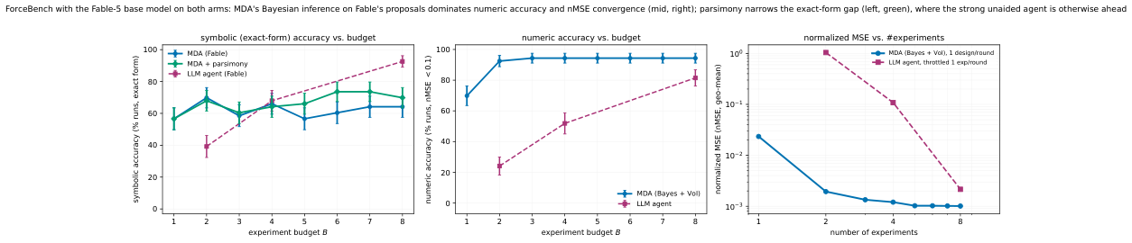
C.9 Example: coulomb world

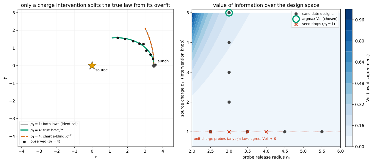
In this section, we visualize behavior of MDA when applied to $\textsc{coulomb}$ world, as shown in Figure 14. On the left, we show what happens when a probe is launched near the source. At unit charge ($p_1{=}1$) the true law $k, q_iq_j/r^2$ and the charge-blind overfit $k/r^2$ trace the same orbit (grey) — fit on unit-charge data, they are identical there, so no probe placement, at any radius or launch, can tell them apart. Turning the source charge to $p_1{=}4$ — a $\mathrm{do}(a)$ on the mechanism — scales the true law's force fourfold (green) while the overfit is unmoved (orange): the orbits split, and that split is what the observations measure.

On the right, we plot the VoI over a 2d slice of the design space, namely the release radius $r_0$ (an initial condition) $\times$ source charge $p_1$ (an intervention knob). The red $\times$ are the seed drops: the unit-charge probes the agent has already collected (the initial, un-designed observations both laws are fit to). VoI is $\approx!0$ all along the unit-charge axis, and rises only with the charge, so MDA's VoI-driven design step reaches for a charge intervention (green ring), not a farther probe. Thus we see that changing a causal (mechanism) knob, not just the initial location, is needed to distinguish a correct law from a curve-fit.

C.10 Example: yukawa world

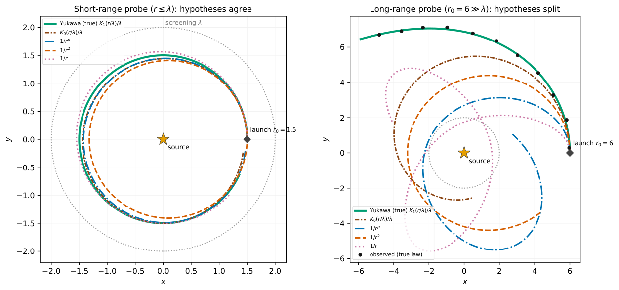
Whereas $\textsc{coulomb}$ 's discriminating design is a charge intervention (Figure 14), $\textsc{yukawa}$ 's is a spatial extrapolation. The screened kernel $K_1(r/\lambda)/\lambda$ and the power laws fit to short-range data are nearly identical for $r\le\lambda$ and diverge only beyond it, so a probe confined within $\lambda$ cannot tell them apart while one reaching past $\lambda$ can (Figure 15). This is why the VoI design reaches for the long-range $r_0{=}5, 6$ drops (Table 5), and why the true kernel only reaches the convex corner of the Pareto frontier (Figure 1b) once such a probe is added.

C.11 Example: discovering hidden particles

In this section we give a simplified example of the $\textsc{dark-matter}$ world, where the challenge is to identify both the number and location of hidden particles.

The model class.

Neutral test probes move in a known static 2D Poisson field: a source of coupling $q$ at position $s$ pulls a probe at $x$ with force $q/(2\pi\lVert x-s\rVert)$ toward $s$, and the field superposes over sources. One visible source of known coupling sits at the origin; the world also contains $K$ hidden sources whose positions and couplings are concealed. A probe released from rest therefore falls not toward the visible source but toward the total mass, so it appears to accelerate toward empty space — the dark-matter tell (Figure 16, middle, arrows). The structure $m$ is the count $K$; its parameters are the $3K$ hidden coordinates and couplings. The design knob $a\in \mathcal{I}$ is the probe launch configuration $(x, y)$, a point in the plane, encoded as a $\mathrm{do}(\cdot)$; we record the probe under position noise $\sigma=0.03$. Because the sources are point masses, not a density field, the forward model is small- $N$ and the whole rung runs on CPU.

The task.

The true world has one visible source ($q=2$ at the origin) and one hidden mass ($q=4$ at $(3.5, 2)$). The method is handed three seed probes released far from the hidden mass, so they feel it only as a weak far-field deflection: enough to reveal that some unseen mass exists, but too little to say where. It must (i) decide how many hidden masses there are, (ii) localize the one that exists, and (iii) choose where to place the next probe. We fit $K\in{0, 1, 2}$ by adaptive-tempering SMC over the hidden coordinates (Algorithm 4, $N_p=1000$) and combine by marginal evidence (§ A.2); $K{=}0$ is a genuine zero-parameter model (visible field only), so comparing it to $K{=}1$ is Bayesian model selection, and comparing $K{=}1$ to $K{=}2$ is Bayesian Occam — a second mass must earn its three parameters against the prior volume they cost.

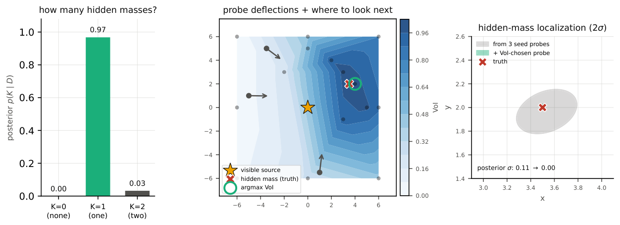
Model selection and localization.

The evidence is decisive (Figure 16, left): $p(K{=}1\mid D)\approx0.97$, with $K{=}0$ excluded outright (its visible-only field cannot bend the probes toward empty space) and $K{=}2$ rejected by Occam (fitting a second, redundant mass buys a negligible likelihood gain for a three-parameter prior-volume penalty). The recovered mass sits at $(3.53, 1.97)\pm(0.13, 0.09)$ with coupling $3.99\pm0.07$ — correct in count, position, and strength. That the count is inferred, not assumed, is the point: this is the latent-existence question (§ 2) — is there an unobserved cause, and how many — answered by evidence.

Where to look, in a 2D design space.

Which placement best localizes the mass? We score each candidate by the query-relevant VoI Equation (9) for a downstream query — a test probe released near the hidden mass, whose outcome depends on the hidden-mass position. The VoI landscape (Figure 16, middle) peaks sharply on the hidden mass: a probe placed there measures it directly, while probes on the far side (visible-dominated) are nearly useless. Running the argmax probe drives $p(K{=}1)$ to $1.0$ and collapses the position posterior from $\sigma\approx0.11$ to $\approx0.01$ (Figure 16, right) — the localization the seed probes could not reach.

D. Chemistry: additional details

D.1 Benchmark

The problem is to learn a static algebraic function of seven controllable inputs (substrate, inhibitor, second substrate and product concentrations, enzyme loading, temperature and pH) to a reaction rate $y$:

$ y = f\big(C_A, C_I, C_B, C_P, \mathrm{Enz}, T, \mathrm{pH};, \theta\big),\tag{18} $

The unknown is which kinetic mechanism is active. There are 9 canonical single mechanisms (Michaelis–Menten, competitive / uncompetitive / noncompetitive / product inhibition, substrate inhibition, Hill cooperativity, Arrhenius temperature dependence, ping-pong bisubstrate), and 48 compound mechanisms, created from combinations of these elementary mechanisms (e.g., ping-pong $\times$ Arrhenius, MM $\times$ competitive $\times$ Arrhenius and Hill $\times$ Arrhenius), yielding a total of 57 rules or worlds. The dataset is divided into easy, medium, and hard tiers, based on the mechanisms used and their corresponding parameters (some of which make the response hard to detect).

Performance of a submitted law is evaluated using the procedure described in ([2], App.C). First we compute the held-out root-mean-squared log-error $\mathrm{RMSLE}=\big[\tfrac1N\sum_{i=1}^{N}\big(\log(1{+}\hat{y}_i)-\log(1{+}y_i)\big)^2\big]^{1/2}$ over $N{=}1000$ test points. Then we compute whether the law is numerically equivalent to the true law using $\textsc{ExAcc}$ $= \mathbb{1}[\mathrm{RMSLE}<\epsilon]$, a quantity they call the "exact accuracy". The released benchmark code uses $\epsilon{=}0.05$ for chemistry (and $0.01$ for physics). Our data-efficiency curves (Figure 3) use the stricter App. C threshold $\epsilon{=}0.01$, whereas the head-to-head Table 9 reports $\epsilon{=}0.05$ to match $\textsc{LLM-AutoSciLab}$ 's published numbers. They also compute symbolic equivalence to the true law using sympy.

D.2 Further results

\begin{tabular}{@l cc cc cc cc@}
\toprule
 {} & \multicolumn{2}{c}{Easy} & \multicolumn{2}{c}{Medium} & \multicolumn{2}{c}{Hard} & \multicolumn{2}{c}{\bf Overall}\\
\cmidrule(lr){2-3}\cmidrule(lr){4-5}\cmidrule(lr){6-7}\cmidrule(lr){8-9}
Method & SA & Ex & SA & Ex & SA & Ex & \bf SA & \bf Ex\\
\midrule
MDA (VoI) & \bf 66.7 & \bf 83.3 & 45.8 & 79.2 & \bf 54.2 & \bf 79.2 & \bf 55.6 & \bf 80.6\\
MDA (Mean) & 54.2 & 79.2 & \bf 58.3 & \bf 87.5 & 33.3 & 66.7 & 48.6 & 77.8\\
\textsc{LLM-AutoSciLab} (us) & 41.7 & 58.3 & 41.7 & 75.0 & 41.7 & 75.0 & 41.7 & 69.4\\
\midrule
\textsc{LLM-AutoSciLab} (reported) & 55.6 & 88.9 & 22.2 & 37.0 & 42.9 & 52.4 & 35.1 & 50.9\\
\bottomrule
\end{tabular}

Table 9 reports symbolic accuracy (SA) and exact accuracy ($\textsc{ExAcc}$, at their $0.05$ threshold for comparability), per difficulty tier and overall, at a max budget of $B{=}60$ experiments. We see that MDA beats their method overall (SA $56$ vs. $42$ and $\textsc{ExAcc}$ $81$ vs. $69$), as well as on every tier. Crucially, MDA wins on the hard tier, where $\textsc{LLM-AutoSciLab}$ 's low-error solutions are numerically accurate but mechanistically meaningless (e.g. recovering $10^{, 0.87\log(0.5\sqrt{\mathrm{Enz}/\dots})}$ at $\mathrm{RMSLE}{=}0.001$, which passes even the strict $0.01$ threshold, yet the symbolic-equivalence check marks it as wrong).

D.3 Ablations

In Figure 17, we show the effects of ablating various parts of the MDA method (36-task subset, $B=60$ experiment budget).

• We start by using vanilla SMC, as in the ModelSMC paper ([23]), combined with Monte Carlo (random sampling) based optimization of the VoI.
• Next we add $\mathcal M$-open exploration. This lifts overall symbolic accuracy $36{\to}50%$ — driven by the easy tier, where the residual-directed re-prompt corrects the single-mechanism form (easy SA $42{\to}75%$). This is the only route to any compound recovery ($0{\to}11%$, since the fixed library of 9 primitives cannot express compound mechanisms). Interestingly, this does not help the hard tier, where the mechanism's signal is too weak under the extreme parameters.
• Next we add CMA-ES optimization of VoI. This sharpens the design, raising exact numerical accuracy $36{\to}42%$ and hard-tier SA $33{\to}42%$.
• Finally we add the ESS-adaptive pool. This lifts overall SA $50{\to}56%$ and hard-tier SA $42{\to}54%$ by evicting the over-elaborated near-duplicates the exploration introduces. Together they turn the ModelSMC base ($36%$ SA) into a method that wins every tier of the fair comparison.

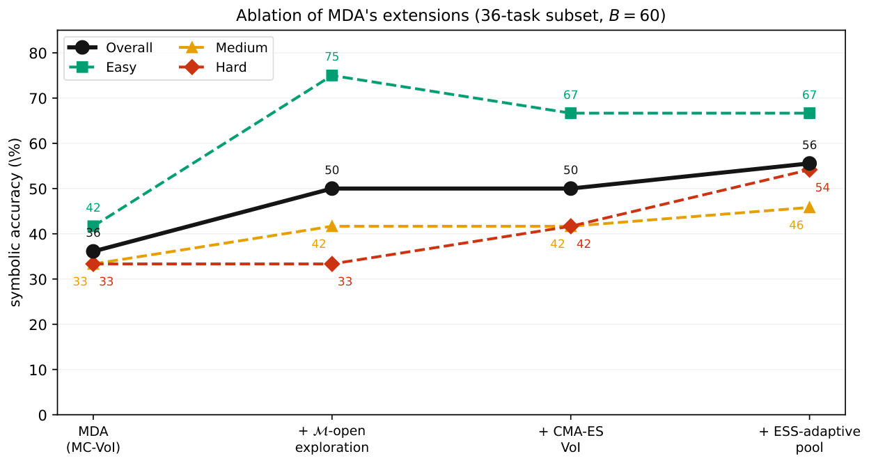
E. NeuronBench

This appendix covers the deterministic form of the benchmark: background on neuron electrophysiology and Hodgkin–Huxley models, the problem specification, the (tractable, synthetic-feature) solution methods, the benchmark results and baselines, and case studies. The stochastic form — where the likelihood becomes intractable — is deferred to Appendix F.

E.1 Primer on neuron electrophysiology

In this section, we give a brief introduction to neuron electrophysiology.

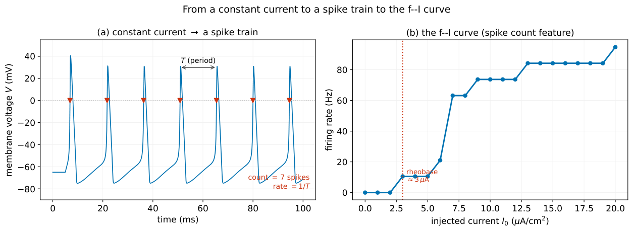
We can view a neuron as a device that turns an injected current into a voltage trace. At rest the membrane voltage $V$ sits near $-65$ mV. A small (sub-threshold) injected current depolarises $V$ a little and it relaxes back — a passive, RC-like response. A large enough (supra-threshold) current triggers an action potential or spike: voltage-gated Na$^+$ channels open regeneratively, $V$ shoots to ${\sim}{+}40$ mV in under a millisecond, then K$^+$ channels open and pull it back down. Spikes are the neuron's output; their count (or rate) as a function of the injected-current amplitude is the f–I curve (frequency–current), the standard input–output summary of a cell: see Figure 18.

Crucially, the behavior of the neuron depends on its inputs, as illustrated in Figure 19. Here we show the voltage over time, under 3 different experimental conditions: the standard model, stimulated with a 10 $\mu A$ step signal, which generates repeating spikes (blue); the same model stimulated with a 2 $\mu A$ step signal, which fails to trigger a response (dotted black); and the model modified by applying TTX blocker and then stimulated with a 10 $\mu A$ step signal, which also fails to trigger a response (red line). This illustrates why experiment design is critical in this domain.

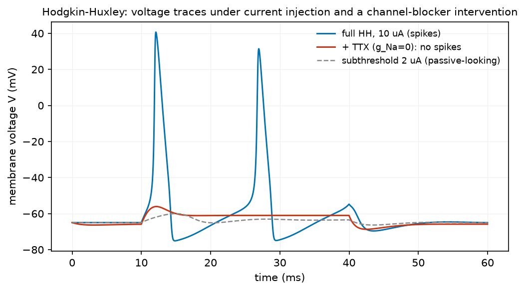
E.2 Primer on Hodgkin-Huxley models

In this section, we give a brief primer on generalized Hodgkin-Huxley models. The model is named after Alan Hodgkin and Andrew Huxley who invented it in 1952 to explain the ionic mechanisms underlying the initiation and propagation of action potentials in the squid giant axon. Since then, the model has been generalized and is widely used to mechanistically explain the spiking behavior of many kinds of neurons. Hodgkin and Huxley received the 1963 Nobel Prize in Physiology or Medicine for this work.

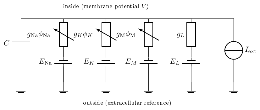
The model they came up with can be represented as an electric circuit, as shown in Figure 20. This example contains Na, K, M and L ion channels, but the generalized model can contain different combinations of the 6 channels listed in Table 11, each of which have their own parameters and dynamics. We can write the generalized model as a set of nonlinear ODEs, which follow from Kirchoff's current law:

$ \begin{aligned} C \frac{d V(t)}{dt} &= I_{\mathrm{ext}}(t) ;-; \sum_{c\in\mathcal C} I_c(t) \quad\text{(a)} \ I_c(t) &= g_c \phi_c(t) (V(t) - E_c) \ \phi_c(t) &= m_c^{p_c}(t) ; n_c^{q_c}(t) ; h_c^{r_c}(t) \ \frac{d x_c(t)}{dt} &= \frac{T_{x, c}^{\infty}(V(t))-x_c(t)}{\tau_{x, c}(V(t))}, ; x \in {m, n, h} \quad\text{(b)} \end{aligned}\tag{19} $

Here $C$ is the capacitance, $V(t)$ is the voltage, $I_c$ is the current for channel $c$, $\mathcal C$ is the set of channels associated with this neuron, and $\phi_c(t)$ is the fraction of the channel that is open. Thus the current in the channel is given by $I_c=g_c, \phi_c, (V-E_c)$: (maximal conductance) $\times$ (fraction open) $\times$ (driving force). The fraction open $\phi_c$ (which changes over time) is based on a product of gating terms — denoted by $m_c$, $n_c$ and $h_c$ — each raised to an integer power ($p_c, q_c, r_c$; how many independent gates the channel has): see Table 11 for the list. Each such gating term $x_c$ relaxes towards a voltage-dependent target $T_{x, c}^{\infty}(V)$ with its own time constant $\tau_{x, c}(V)$ (fast for activation, slow for inactivation), given by

$ T_{x, c}^{\infty}(V) =\frac{\alpha_x(V)}{\alpha_x(V) + \beta_x(V)}, ; \tau_{x, c}(V) =\frac{1}{\alpha_x(V) + \beta_x(V)}\tag{20} $

where expressions for $\alpha_x$ and $\beta_x$ can be found at https://en.wikipedia.org/wiki/Hodgkin-Huxley_model. As example, the classic spiker is the following three-channel model

$ C\dot{V} = I_{\mathrm{ext}}

• g_{\mathrm{Na}}m_{\mathrm{Na}}^3 h_{\mathrm{Na}}, (V{-}E_{\mathrm{Na}}) - g_K n_K^4, (V{-}E_K) - g_L, (V{-}E_L) $

Here the Na$^+$ channel carries an activation gate $m_{\mathrm{Na}}$ (cubed) and an inactivation gate $h_{\mathrm{Na}}$, and the K$^+$ channel a single activation gate $n_K$ (to the fourth); Table 10 summarises the three. The names $m, n, h$ are historical: what actually distinguishes a gate is its target curve $T_{x, c}^{\infty}(V)$ (whether it opens or closes as $V$ rises) and its time constant $\tau_{x, c}(V)$. It is the separation of timescales — fast $m_{\mathrm{Na}}$ activation admitting Na$^+$ for the upstroke, before the slower $h_{\mathrm{Na}}$ inactivation shuts it off and the slower $n_K$ activation repolarises — that makes the spike a transient, regenerative event.

\begin{tabular}{@lllll@}
\toprule
gate & channel & role & target $T_{x, c}^{\infty}(V)$ & speed \\
\midrule
$m_{\mathrm{Na}}$ & Na$^+$ & activation & rises with depolarisation & fast \\
$h_{\mathrm{Na}}$ & Na$^+$ & inactivation & \emph{falls} with depolarisation & slow \\
$n_K$ & K$^+$ & activation & rises with depolarisation & slow \\
\bottomrule
\end{tabular}

It is worth noting that HH is only one point on a spectrum of models at different levels of abstraction. There are more detailed stochastic models that capture individual cellular responses at a more granular level. There are also simplified models, such as the two-variable FitzHugh–Nagumo model, and the leaky integrate-and-fire model. Finally, if we set the membrane time constant to zero and binarise the output, we get the McCulloch–Pitts unit ([53]), $y=\phi(\sum_i w_i x_i-b)$, which is the basis of artificial neural networks. So there is no single "true model". Instead, scientists seek the coarsest valid causal abstraction that is sufficient for the things they want to understand or predict ([54, 55]).

\begin{tabular}{@l l l p{3.7cm} l@}
\toprule
Channel & carries & current & role in the response & blocker (a $\mathrm{do}$) \\
\midrule
Na$^+$ & sodium &
$I_{\mathrm{Na}}=g_{\mathrm{Na}}m_{\mathrm{Na}}^3 h_{\mathrm{Na}}\, (V{-}E_{\mathrm{Na}})$ &
regenerative spike \emph{upstroke} & tetrodotoxin (TTX) \\
K$^+$ (delayed rectifier) & potassium &
$I_K=g_K n_K^4\, (V{-}E_K)$ &
\emph{repolarises} the spike & TEA \\
Ca$^{2+}$ (high-threshold) &calcium &
$I_{\mathrm{Ca}}=g_{\mathrm{Ca}}m_{\mathrm{Ca}}^2 h_{\mathrm{Ca}}\, (V{-}E_{\mathrm{Ca}})$
 {} & \emph{alternative}, slower spike upstroke & cadmium (Cd) \\
M-type K$^+$ & potassium &
$I_{\mathrm{M}}=g_{\mathrm{M}}\, m_{\mathrm{M}}\, (V{-}E_K)$
 {} & slow; \emph{spike-frequency adaptation} & XE991 \\
A-type K$^+$ (transient) & potassium &
$I_{\mathrm{A}}=g_{\mathrm{A}}m_{\mathrm{A}}^p h_{\mathrm{A}}\, (V{-}E_K)$
 {} & transient outward; \emph{delays} firing onset & 4-AP \\
leak & mixed &
$I_L=g_L\, (V{-}E_L)$
 {} & sets the \emph{resting potential}; passive & --- \\
\bottomrule
\end{tabular}

E.3 Our benchmark

We design a benchmark, $\textsc{NeuronBench}$, by creating 6 "mystery neurons", each composed of a plain Na $+$ K $+$ leak spiker plus one extra membrane mechanism, chosen from the list in Table 12: five are novel mechanisms and the sixth is a recallable textbook M-current control. Each of the five novel mechanisms is deliberately tuned to be silent under every textbook probe, i.e., the plain and novel neurons fire identically to standard current steps and channel blockers. This requires the agent to propose novel experimental protocols that it has not already memorized.

The task

The agent is told that it will be presented with some voltage trace data from a neuron of unknown type, and is asked to propose various candidate mechansims (the exact prompts are shown in Appendix H.3). It is also given the menu of stimulation protocols (Table 13) and channel blockers, and a fixed experiment budget. From a handful of designed experiments it must (i) propose its own candidate mechanisms $m$ and return a posterior $p(m\mid \mathcal{D})$ over them, and (ii) forecast the cell's response to held-out interventions it never ran. The truth is never revealed to the agent; it is used only for scoring. (A solver may of course restrict its hypothesis space — e.g. MDA fits a pool of conductance archetypes — but the benchmark neither supplies nor assumes an enumerated candidate set.)

Evaluation.

The task is counterfactual trajectory forecasting: on a disjoint set of held-out protocols the agent never ran, it must predicts the cell's response — a spike count and a voltage trace per protocol. Because the hypothesis space is open we score behaviour, not model labels, on two levels. (i) The spike-forecast MSE (the headline metric): the mean-squared error of the predicted test-window spike counts. (ii) The feature-forecast MSE (a secondary, finer metric for model-based deep-dives): the standardised MSE, over the per-trace summary feature vector $s(y)$ of Equation 22 between the agent's predicted trace and the truth.

Npte that the feature-forecast requires predicting a full trace, which is then converted to summary features. Generating a trace is hard to do for a pure LLM based forecaster, but is easy for a model-based one. We reduce the prediction to a set of features in order to make the comparison to ground truth more meaningful (see Appendix E.4).

Specification of the novel channels.

Each novel channel has roughly the same gated form as the textbook ones:

$ I_Z = g_Z, m_Z^{p}, h_Z^{q}, (V-E_Z), \quad T_{m, Z}^{\infty}(V)=\sigma!\Big(\tfrac{V-V^m_{1/2}}{k_m}\Big), \quad T_{h, Z}^{\infty}(V)=\sigma!\Big(!-\tfrac{V-V^h_{1/2}}{k_h}\Big),\tag{21} $

with $\sigma(u)=1/(1+e^{-u})$ the logistic (Boltzmann) sigmoid, half-voltages $V^m_{1/2}, V^h_{1/2}$, slopes $k_m, k_h{>}0$, and fixed time constants $\tau_m, \tau_h$: activation rises with $V$ and inactivation falls, while a negative activation slope $k_m{<}0$ instead makes the channel hyperpolarisation-activated (as for $I_h$), and an inactivation half-voltage $V^h_{1/2}$ below rest makes it de-inactivated by hyperpolarisation (available only after a hyperpolarising pre-pulse). This Boltzmann form is generic across the novel channels but is not the textbook parameterisation shown in Equation 20, which are monotonic curves of the same qualitative shape but not identical logistic sigmoids.

::: {caption="Table 12: The six worlds of NeuronBench. Each current is added to a Na + K + leak spiker via Equation 21; the row label is the Figure 4 panel name. †the activation / inactivation columns are the tuples ($V_1/2$, k, tau, power) and ($V_1/2$, k, tau) of Equation 21. Conductances $g_Z$ in mS / cm^2; reversals $E_Z$, half-voltages and slopes in mV; time constants in ms; p, q are gate powers (q=1 when an inactivation gate is present, else 0). All are tuned to be indistinguishable from the plain spiker under textbook steps and blockers and separable only by the matched non-textbook protocol in the last column (a hyperpolarising conditioning pre-pulse for the de-inactivating currents). na-fatigue adds no channel: it slows the inactivation of the existing Na^+ gate $h_Na$. The $I_M$ control is a standard non-inactivating $K^+$ current the LLM can name and probe."}

:::

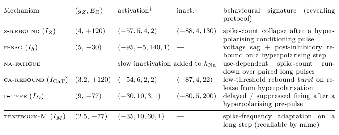
Design space.

The agent gets to control the external current $I_{\mathrm{ext}}(t)= x_t$ injected at each step. In our benchmark, we assume the current is chosen from one of the 9 sequence options in Table 13. In principle the agent can also apply a single channel blocker (tetrodotoxin (TTX) zeroing $g_{\mathrm{Na}}$, TEA zeroing $g_{\mathrm{K}}$, cadmium (Cd) zeroing $g_{\mathrm{Ca}}$, or none), giving a nominal $9\times4$ actions. But the novel mechanisms are by construction silent under blockers as well as under textbook steps — a blocker deletes a channel branch equally in the plain and novel cells, so it cannot separate them — so the blockers are non-discriminating for these worlds. We therefore report all experiments over just the $9$ current-clamp protocols (blockers remain available in the released benchmark and the interactive app, but are unused in the runs, for simplicity).

::: {caption="Table 13: The nine-protocol menu of external currents that can be applied over which VoI is enumerated on NeuronBench. Each protocol is a sequence of (duration, amplitude) current segments; a leading hyperpolarising segment is a conditioning pre-pulse. Rows 1–4 are standard current-clamp steps; rows 5–9 are the non-textbook protocols that expose the hidden mechanisms of Table 12 — exactly one is decisive for each, so only a designed (VoI-chosen) experiment identifies the mechanism."}

:::

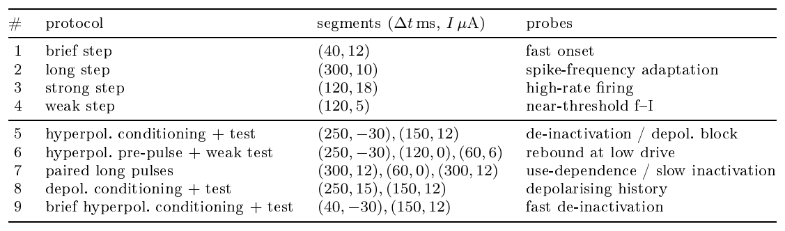
Interactive app.

Figure 21 shows a screenshot for a web app we built that lets users try this benchmark for themselves. The app is available at https://github.com/murphyk/neuronbench.

E.4 The likelihood: summary features, not the raw trace

Because a spike is a ${\sim}1$ ms all-or-none event, a sub-millisecond timing mismatch between model and data produces a ${\sim}100$ mV pointwise error even for an essentially correct model. Hence a likelihood that factorizes over time steps, as in Equation 4, is dominated by nuisance spike-timing noise and is useless for spiking data. We instead use a feature (synthetic / simulation-based) likelihood, the standard choice in this field. That is, we use $p(y_{1:T} | \xi, m, \theta) \propto \prod_{j=1}^J p(s_j(y_{1:T})| \xi, m, \theta)$, where $s_j$ is the $j$ th feature (a scalar) derived from the entire trajectory $y_{1:T}$.

Deterministic synthetic likelihood.

The above synthetic likelihood does not factorise over time. However, because we assume the latent dynamics are deterministic and the initial state is known, it is tractable to compute: we solve the ODE for $z_{1:T}$, read off the predicted features $s_j(m, \theta)=s_j(z_{1:T})$, and evaluate the kernel in closed form. By contrast, if the dynamics are stochastic, the likelihood $p(s_j(y) \mid m, \theta)=\int p(s_j(y) \mid z_{1:T}), p(z_{1:T}\mid m, \theta), dz_{1:T}$ has no closed form, so we have to marginalize out over the latent paths, as we discuss in Appendix F.1.

The summary statistics.

The summary statsitic we use are spike counts in the test and conditioning windows, their use-dependent run-down, within-pulse adaptation, and two sub-threshold voltage summaries, as illustrated in Figure 22. These are computed as follows:

$ s(y)=\Big(\underbrace{n_{\mathrm{test}}}{\text{test spikes}},
\underbrace{n{\mathrm{pre}}}{\text{pre-pulse spikes}},
\underbrace{n{\mathrm{pre}}-n_{\mathrm{test}}}{\text{run-down}},
\underbrace{n^{\mathrm{early}}{\mathrm{test}}-n^{\mathrm{late}}{\mathrm{test}}}{\text{adaptation}},
\underbrace{\min_t V(t)}{V{\min}},
\underbrace{\bar{V}{\mathrm{end}}}{\text{steady state}}\Big),\tag{22} $

where $n_{\mathrm{test}}, n_{\mathrm{pre}}$ count upward zero-crossings of $V$ in the test window (after any conditioning pre-pulse) and before it, $n^{\mathrm{early}}{\mathrm{test}}{-}n^{\mathrm{late}}{\mathrm{test}}$ splits the test window in half, and $\bar{V}_{\mathrm{end}}$ is the mean voltage over the steady-state tail of the trace (the final few percent, after the stimulus ends). This is chosen so that both the rate-signature worlds ($\textsc{na-fatigue}$, $\textsc{textbook-M}$) and the sub-threshold/burst worlds ($\textsc{h-sag}$, $\textsc{ca-rebound}$) leave a signal.

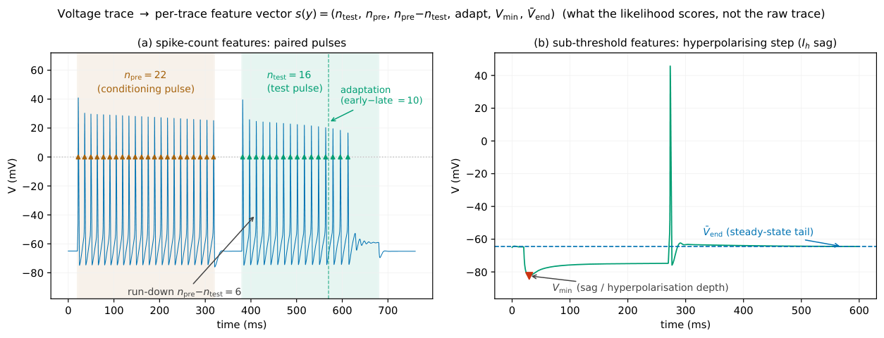
Gaussian likelihood.

For real-valued summaries we use a Gaussian kernel

$ p(y_{1:T}\mid m, \theta) = \prod_j \mathcal{N}(s_j(y_{1:T}) | s_j(z_{1:T}), \sigma_j)\tag{23} $

where $z_{1:T}=\text{unroll}(m, \theta, z_0)$ is the trajectory deterministically generated by solving the ODE defined by $m$ and $\theta$ from the initial condition $z_0$.

Poisson likelihood.

In some cases, the features are just the spike counts ${n_k}$ at different input currents $\xi_k=a_k$. Since this is a set of non-negative integers, the natural observation model is a product of Poissons:

$ p(y_{1:T}\mid { \xi }, m, \theta);\propto; \prod_k \mathrm{Poi}!\big(n_k(y_{1:T}), ;, \lambda_k(m, \theta)\big), \qquad \lambda_k;=;n_k\big(z_{1:T}(m, \theta, \xi_k)\big).\tag{24} $

Here the rate $\lambda_k$ of the $k$-th count is obtained by running the candidate model $m$ forward — solving its ODEs under protocol $a_k$ to get the voltage trace $z_{1:T}=V_\theta(\cdot;a_k)$ — and then applying the same spike-count feature map $n_k(\cdot)$ used on the data, i.e. counting upward threshold crossings of that simulated trace. That scalar predicted count is the Poisson mean; the observed recording supplies the Poisson "data" $n_k(y_{1:T})$. So the deterministic model sets the mean spike count per protocol and the Poisson supplies the trial-to-trial spike-count dispersion (in practice we average a few repeats per protocol).

Example: ca-rebound.

In this section, we visualize the predictive distribution $p(y_{1:T}|m)$ for two different hypotheses $m$ — the plain Na+K+L neuron, and the correct Na+K+L+Z neuron — and show the resulting summary statistics. These results are for the $\textsc{ca-rebound}$ world, and are obtained under a VoI-designed experiment $\xi$ (here a hyperpolarising pre-pulse that de-inactivates the hidden Ca2+ current, then a weak test). Figure 23 visualizes a trace $y_{1:T}$ and its summary statistic (4 spikes), followed by a prediction $E[y_{1:T}|m, \xi]$ and the summary statistics we derive from each prediction (2 spikes and 4 spikes). We see that despite the trajectory being reduced (in this case) to a single integer, $s(y_{1:T})$, the synthetic likelihood can discriminate the correct model from the incorrect one, if the design $\xi$ is chosen properly.

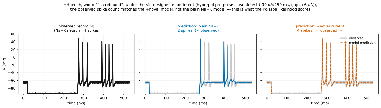
E.5 Parameters and priors.

Table 14 lists what is inferred and under what prior. The only free parameters are the maximal conductances $g_c$ of the present channels; each is given an independent log-normal prior centred on its literature nominal value, with a log-space SD of $0.7$ — a $1\sigma$ band of roughly $[nominal/2, \ nominal {\times}2]$, deliberately broad since the target is a real cell of unknown size. The membrane capacitance, reversal potentials, and the voltage-dependent gating kinetics $T_{x, c}^{\infty}(V), \tau_{x, c}(V)$ are held fixed (a channel is its kinetics; only its density $g_c$ is free), and the feature-kernel tolerances $\sigma_j$ are the fixed observation model.

\begin{tabular}{@llll@}
\toprule
Quantity & Symbol & Prior / value & Role \\
\midrule
\multicolumn{4}{@l}{Inferred (only for channels present in the structure $m$):}\\
Na$^+$ conductance & $g_{\mathrm{Na}}$ & $\mathrm{LogNormal}(\log 120,  0.7^2)$ & spike upstroke \\
K$^+$ (delayed rect.) & $g_{\mathrm{K}}$ & $\mathrm{LogNormal}(\log 36,  0.7^2)$ & repolarisation \\
Ca$^{2+}$ (high-thr.) & $g_{\mathrm{Ca}}$ & $\mathrm{LogNormal}(\log 12,  0.7^2)$ & alt. spike carrier \\
A-type K$^+$ (transient)& $g_{\mathrm{A}}$ & $\mathrm{LogNormal}(\log 45,  0.7^2)$ & onset delay \\
M-current (slow K$^+$) & $g_{\mathrm{M}}$ & $\mathrm{LogNormal}(\log 1.0,  0.7^2)$ & spike-freq. adaptation \\
leak & $g_{\mathrm{L}}$ & $\mathrm{LogNormal}(\log 0.3,  0.7^2)$ & resting potential \\
\midrule
\multicolumn{4}{@l}{\emph{Fixed (not inferred):}}\\
capacitance & $C$ & $1.0 \mu$ F/cm$^2$ & membrane \\
reversal potentials & $E_{\mathrm{Na/K/L/Ca}}$ & $+50 / -77 / -54.4 / +120$ \, mV & driving forces \\
gating kinetics & $T_{x, c}^{\infty}(V), \tau_{x, c}(V)$ & Hodgkin--Huxley forms & channel identity \\
\midrule
\multicolumn{4}{@l}{Observation model (feature-kernel tolerances $\sigma_j$):}\\
sub-threshold count & $\sigma$ & $0.3$ spikes (tight; enforces rheobase) & likelihood \\
supra-threshold count & $\sigma$ & $1.2$ spikes & likelihood \\
input resistance & $\sigma$ & $0.06$ mV/pA & likelihood \\
\bottomrule
\end{tabular}

E.6 Results on the benchmark

Figure 4 shows the results of MDA and the LLM baseline on $\textsc{NeuronBench}$. For these results, we used the Poisson likelihood on the spike count, as in Equation 24. We see that MDA is substantially more data efficient.

E.7 Model selection deep dive

In this section, we give a worked example of model selection, to better understand how MDA works. We focus on the $\textsc{h-sag}$ world. The LLM is shown only the phenotype (a depolarising sag during hyperpolarisation, then a rebound) and proposes the candidate channels: HCN/ $I_h$, T-type Ca$^{2+}$, Kir, A-type K$^+$, and persistent Na$^+$, which map onto four distinct dynamical hypotheses ${I_h, \ \text{T-type}, \ \text{D-type K}, \ \text{plain}}$. This is genuinely $\mathcal{M}$-open: the phenotype is consistent with several real channels (all can rebound), so proposing them is correct, not a mistake, and only an experiment can decide. A textbook depolarising input step leaves all four candidates identical (posterior unmoved from the uniform prior), whereas the VoI-designed hyperpolarising probe concentrates the posterior on $I_h$ in one shot. Figure 24(a) shows why: under that probe only $I_h$ produces the depolarising sag; the others stay pinned at the hyperpolarised floor. After discovering the right model structure, SMC continues to refine the posterior over the parameters, as shown in Figure 25.

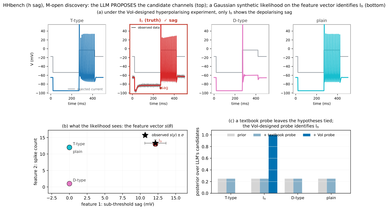
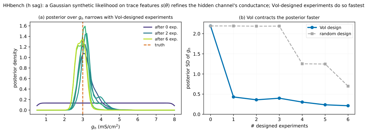
E.8 Learning summary statistics using a 1d CNN

In this section we give a concrete example of the approach discussed in Appendix A.4 for learning a set of summary statistics. In $\textsc{NeuronBench}$ we already know the "right" hand-crafted answer, namely the features shown in Equation 22, but this section shows how a learning based approach can give comparable performance; we will use this in earnest for the stochastic benchmark in Appendix F.

Extracting summary features using a neural network.

We replace $s(y_{1:T})$ with a learned encoder $s_{\phi}(y_{1:T})$ which we train as follows: (1) simulate a bank of $(m, \theta)!\to!y_{1:T}$ raw voltage traces under the design protocol menu; (2) train a small 1-D CNN encoder $s_\phi(y_{1:T})\in \mathbb{R}^d$ with two supervised heads — classify the channel structure $m$ (four candidates, as in Figure 24) and regress its conductance $g$ — on that bank; the supervised targets are what forbid collapse. The two heads are used only to train the encoder — the softmax over structures is a discriminative posterior $p(m\mid y)$, not a likelihood, and both heads are discarded at inference. What we keep is the penultimate-layer embedding $s_\phi(y_{1:T})\in \mathbb{R}^d$ ($d{=}8$), which plays exactly the role of the hand-crafted feature vector of Equation 22.

The likelihood on the learned summary.

We then use the multivariate Gaussian likelihood in Equation 11 to define $p(s|m, \theta)$. This is the multivariate generalisation of the per-feature Gaussian kernel of Equation 23: the deterministic hand-feature case reads the mean off a single rollout with hand-set tolerances $\sigma_j$, whereas the learned (and stochastic) case estimates both the mean and the covariance from the $R$ simulations already drawn for the likelihood. Equation 11 plugs into the model-SMC unchanged, model selection being driven by the log-density gap $\log \mathcal{N}(s_\phi(y)\mid\mu_a, \Sigma_a) -\log \mathcal{N}(s_\phi(y)\mid\mu_b, \Sigma_b)$ between candidates.

Training cost.

The encoder is deliberately tiny — three $1$-D convolutional blocks ($1!\to!16!\to!32!\to!32$ channels) into an $8$-dimensional embedding with a classification and a regression head — so both the data and the compute are negligible. The training bank is $350$ simulated traces per candidate structure ($1400$ total for the four ${I_h, \text{T-type}, \text{D-type}, \text{plain}}$ hypotheses of Figure 24), split $80/20$ into $1120$ train / $280$ test; each trace is a single forward solve under the protocol menu, downsampled to ${\sim}750$ samples. Training runs for $40$ epochs (batch $64$, Adam at $2!\times!10^{-3}$) and completes in about a minute on a laptop CPU/MPS — no GPU cluster. The simulations dominate the wall-clock, and they are the same rollouts already drawn for the synthetic likelihood, so the marginal cost of learning $s_\phi$ over hand-specifying it is essentially free.

Amortized encoder.

For the full benchmark, the set of hypotheses can change across worlds and even across steps. To amortize the cost of training different neural nets, we pre-train a single 1D-CNN over over multiple models sampled from the prior; specifically we use the channel-archetype family. Because the convolutional encoder ends in global average pooling it is protocol-length agnostic, so one encoder serves every world, protocol, and candidate pool without needing retraining. (Only the Gaussian moments of Equation 11 are re-estimated per candidate at scoring time.)

Results.

In Figure 26(a), we show that, on held-out traces, the learned summary identifies the hidden channel with $100%$ accuracy — above the hand-crafted $[\text{sag}, \text{spike-count}]$ baseline ($92%$) — and recovers the conductance to $0.56\ \mathrm{mS/cm^2}$ mean absolute error. Here the two hand features are the sub-threshold "sag" — the slow depolarising recovery from the trough during a hyperpolarising step, the signature of the hyperpolarisation-activated inward current $I_h$ (HCN) — and the spike count; together they discriminate the four candidate channels.

Figure 26(b) asks which windows the learned encoder actually relies on, via an occlusion analysis: we mask each time window of the input and measure the resulting drop in the $I_h$ logit. (We use occlusion rather than a raw input-gradient saliency because the latter is nearly uniform for this network — a known pathology of vanilla saliency — and so localises nothing.) The importance concentrates on the spike windows — the rebound burst after the hyperpolarising release and the depolarising spike train (mean importance $0.54$) — and is markedly lower across the sub-threshold sag phase ($0.20$) and the quiescent stretches ($0.25$). So the network rediscovers that the discriminative signal lives in the firing pattern, the ${n_k}$ spike-count features.

F. NeuronBenchStoch

F.1 Stochastic latent dynamics: background

The worlds above use a deterministic Hodgkin–Huxley forward model, so the likelihood is available in closed form (Appendix E.4). Real neurons are stochastic: with a finite number of ion channels, gating fluctuates (channel noise), the latent dynamics become an SDE. This is the regime real experiments occupy, and the one setting our other benchmarks (deterministic ODEs $+$ observation noise) do not exercise.

To create a stochastic neuron, we add finite- $N_{\text{noise}}$ channel noise via the Fox–Lu diffusion approximation ([56]), with the channel count $N_{\text{noise}}$ tuning the intrinsic noise from near-deterministic ($N_{\text{noise}}!\to!\infty$) to strongly stochastic.

In more detail, each gate $x_c$ is really an ensemble of $N_{\text{noise}}$ two-state ion channels, each switching open $\leftrightarrow$ closed as a continuous-time Markov chain with the voltage-dependent rates $\alpha_x(V), \beta_x(V)$ of Equation 20; the deterministic HH gating ODE is the $N_{\text{noise}}!\to!\infty$ mean-field limit of the open fraction. The Fox–Lu diffusion approximation ([56]) keeps finite $N_{\text{noise}}$ by replacing that mean field with a Langevin (stochastic differential) equation — the deterministic drift plus a Gaussian channel-noise term whose variance scales as $1/N_{\text{noise}}$:

$ d x_c = \big[\alpha_x(V)(1-x_c) - \beta_x(V), x_c\big], dt ;+; \sqrt{\tfrac{\alpha_x(V)(1-x_c) + \beta_x(V), x_c}{N_{\text{noise}}}};, dW_t, \qquad x\in{m, n, h},\tag{25} $

with $dW_t$ an independent Wiener increment per gate. The diffusion coefficient is the sum of the two transition fluxes divided by $N_{\text{noise}}$ (the system-size / $\Omega$-expansion correction to the channel master equation), so more channels means smaller fluctuations and $N_{\text{noise}}!\to!\infty$ recovers the deterministic gate. We integrate Equation 25 by Euler–Maruyama and substitute the noisy gates into the membrane equation 19a, making $N_{\text{noise}}$ a single knob from near-deterministic to strongly stochastic. Fox–Lu is the standard cheap channel-noise model; see [57] for how it compares to exact Markov-chain channel simulation.

F.2 The benchmark

We convert the deterministic six-world $\textsc{NeuronBench}$ (Appendix E.3) into a stochastic form, $\textsc{NeuronBenchStoch}$, changing only what a finite channel count forces — the worlds, the hidden mechanisms, the design pool, and the scoring are otherwise inherited unchanged. Relative to the deterministic benchmark the differences are:

• Stochastic latent dynamics. The gates evolve by the Fox–Lu SDE Equation (25) rather than the deterministic HH ODE Equation (19a a), with the channel count $N_{\text{noise}}$ as a single noise knob. We sweep a noise ladder $N_{\text{noise}}\in{50, 100, 300, 1000, 3000}$ from strongly stochastic to near-deterministic; unless noted we use $N_{\text{noise}}{=}100$ (fairly noisy), and $N_{\text{noise}}!\to!\infty$ recovers the deterministic benchmark.
• Partial, noisy observation. An experiment returns the membrane voltage with additive Gaussian noise ($\sigma{=}2$ mV), sub-sampled every ${\sim}4$ ms. The deterministic benchmark also returns a sub-sampled trace, so sub-sampling itself is not the difference; what changes is that the trace now carries observation noise ($\sigma{=}2$ mV) and is sampled ${\sim}40\times$ more coarsely (${\sim}4$ ms vs. the deterministic ${\sim}0.1$ ms), the two together making $p(y\mid m, \theta)$ intractable.
• Intractable likelihood. The latent path must be marginalised (Appendix F.3), so the closed-form Gaussian likelihood Equation (4) of the deterministic benchmark is unavailable — the agent estimates $p(y\mid m, \theta)$ by simulation (particle filter or synthetic likelihood).
• Repeat-aware design space. The design space is optionally expanded beyond the one used in the deterministic benchmark to allow for repeating a given experiment, i.e., a design is a $(\text{current protocol}, \ \text{num. repeats})$ choice. Running a protocol $r$ times costs $r$ units and averages the channel noise down ${\sim}1/\sqrt r$ (Appendix F.5). Repeating the informative protocol is the experimentalist's response to noise, a design axis absent when the cell is deterministic.

Everything else is unchanged: the same six worlds and hidden mechanisms, the same disjoint held-out set of $6$ test protocols the agent never runs, and the same two scoring metrics — the headline spike-forecast MSE and the secondary feature-forecast MSE on the summary vector $s(y)$ of Equation 22 — now evaluated against the noisy cell, with each held-out target estimated as the mean over $200$ independent stochastic rollouts. This defines $\textsc{NeuronBenchStoch}$.

F.3 Likelihoods

The marginal likelihood for model $m$ is given by

$ Z_m = p(y_{1:T}\mid m, \theta)=\int p(y_{1:T}\mid z_{0:T}, m, \theta);p(z_{0:T}\mid m, \theta);dz_{0:T}, $

where $y_{1:T}$ is the observed voltage trace and $z_{0:T}$ the latent gating path. This requires marginalising over the stochastic latent path $z_{0:T}$ — a high-dimensional path integral with no closed form, because the Fox–Lu transition density $p(z_t\mid z_{t-1})$ is itself intractable. Below we discuss how to approximate this integral using a bootstrap particle filter (Algorithm 5), as well as various other faster approximations.

Particle filtering.

The agent fits a stochastic state-space model Equation 2 where the latent state $z_t=(V_t, {x_c(t)})$ (voltage and gates) evolves by the discretised Fox–Lu transition $p(z_t\mid z_{t-1}, \xi)$ of Equation 25 and 19a, and the voltage is observed with Gaussian noise, $y_t\sim \mathcal{N}(V_t, \sigma^2)$. Candidate models $m$ differ in structure (which channels are present) and in the conductances $\theta$; the channel count $N_{\text{noise}}$ (the noise scale) is a known part of the model here. The one-step transition density $p(z_t\mid z_{t-1}, \xi)$ has no closed form — it is a nonlinear diffusion over the interval — but the bootstrap particle filter never needs it. It only samples the transition (one Euler–Maruyama step, i.e. a Gaussian draw on the gates, Equation 25) as its proposal, and only evaluates the tractable observation density $\mathcal{N}(y_t\mid V_t, \sigma^2)$ to reweight the particles, from which the marginal likelihood $Z_m$ can be estimated. So the intractable-likelihood regime needs only a simulator of the latents plus an evaluable observation model, exactly what a mechanistic ODE/SDE provides — no transition density is ever computed.

Why the deterministic likelihood breaks.

To illustrate why we cannot just use a deterministic ODE model (and hence a deterministic likelihood, as we did in Equation 4), we consider a simple example where we need to distinguish just two hypotheses: a plain Na/K cell vs the novel $\textsc{h-sag}$ model $I_h$ defined in Table 12. The noisy voltage traces from the two hypotheses are shown in Figure 27 — the $I_h$ sag is subtle relative to the channel noise, so they overlap. In Figure 28(a) we plot the log-evidence gap, $\log Z_1 - \log Z_2$, vs noise level $N_{\text{noise}}$, where $Z_1$ is the evidence for the $I_h$ hypothesis and $Z_2$ for the alternative Na/K hypothesis. We see that a likelihood that treats the intrinsic channel noise as zero degrades as the noise grows and, at $N_{\text{noise}}{=}1000$ channels, inverts: it confidently selects the wrong mechanism. By contrast, the particle filter algorithm in Algorithm 5, which propagates the latent gating SDE with $N_z$ particles and weights each by the observation, stays robustly correct at every noise level.

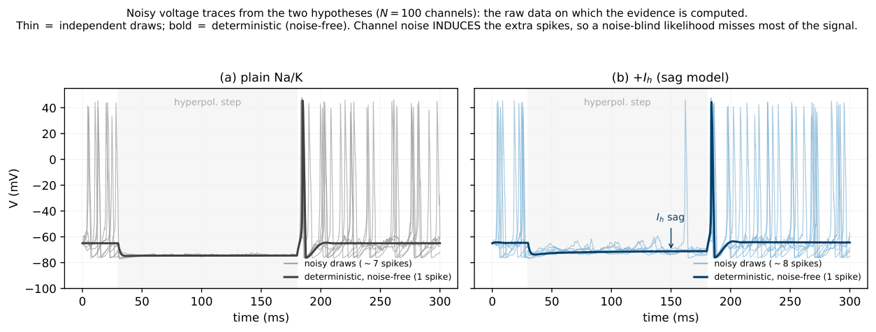
A learned-summary synthetic likelihood as a cheap surrogate.

The particle filter is accurate but costly ($\sim 4$ s per candidate model per experiment, $N_z{=}600$). We therefore use a learned summary statistic, using the 1d CNN architecture discussed in Appendix E.8 to compute $s_{\phi}(y|m, \theta)$. We then fit the Gaussian synthetic likelihood using simulation, as in Equation 11. As an initial proof of concept, we first apply this to the case where there are just two hypotheses to distinguish, a plain neuron vs a plain+ $I_h$ neuron. We fit the model as above and then compute the log-evidence gap, $\log(Z_1/Z_2)$, where $Z_1=p(\mathcal{D}|m_1)$ and $Z_2=p(\mathcal{D}|m_2)$ are the evidences for the two models. We plot this for different datasets produced at different noise levels. As we show in Figure 28(b), the learned synthetic likelihood reproduces the particle filter's decision in $\sim 10^4\times$ less compute. For the full benchmark, the set of hypotheses can change across worlds and even across steps, so we use the amortized encoder from Appendix E.8.

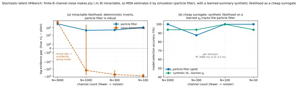
Which observation model?

In this section we consider a simplified version of the 6 stochastic worlds where we only have two hypotheses (truth and a distractor). We use $N_{\text{noise}}{=}100$ latent channels, so the dynamics are fairly stochastic. We consider the deterministic likelihood (one noiseless rollout $+$ Gaussian voltage noise), the bootstrap particle filter on the raw voltage, and a synthetic likelihood on the feature vector $s(y)$ of Equation 22, estimated by simulation, as in Equation 11. The results are shown in Figure 29. We see that the voltage particle filter is the robust generalist: correct on five of six worlds and, crucially, it never inverts (its one weak world is the SNR-limited $\textsc{na-fatigue}$, where it sits at chance). The deterministic likelihood does more than degrade — on $\textsc{ca-rebound}$ it confidently inverts (wrong on every seed), reproducing the single-world failure of Figure 28 in a fresh world: treating each voltage sample as independent Gaussian evidence accumulates spike-timing jitter into a large, wrong gap. The feature likelihood is complementary: it stays above chance on every world and edges the particle filter on the spike-rate world $\textsc{na-fatigue}$ (where the raw-voltage PF is at chance), but is weaker on the worlds whose discriminating signal is a sub-threshold or timing shape ($\textsc{h-sag}$, $\textsc{d-type}$) that the summary vector compresses. There is thus no single best observation model: shape signatures want the voltage filter, spike-rate signatures want the feature likelihood, and neither escapes the overconfidence that sinks the deterministic one on $\textsc{ca-rebound}$ — which is what motivates the section below.

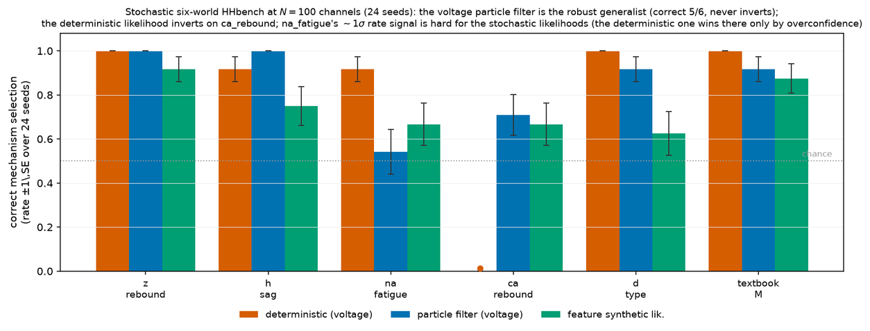
Auto-selecting the observation model.

Because no single observation model wins on every world (Figure 29), the agent should hold both the feature synthetic likelihood and the voltage particle filter and pick per world — and it can do so without knowing the truth. Before committing to an experiment it runs a cheap probe: on the world's discriminating protocol it simulates single experiments from each candidate in turn and measures how often each observation model's log-evidence gap identifies the generator, averaged over which candidate generated the data. This is pure discrimination power — which likelihood best tells the hypotheses apart, never peeking at the truth.

Formally this is the cost-aware observation-model selection of Equation 12, applied here over $o\in{\text{PF}, \ \text{feat}}$: the agent estimates each $\mathrm{MI}_o$ by the truth-free discrimination probe above and, charging the PF its extra compute ($\mathrm{cost}(\text{PF})/\mathrm{cost}(\text{feat})!\approx! N_z/R!\gg!1$), defaults to the cheap feature likelihood and pays for the filter only where its discrimination clearly justifies it. Ignoring cost it reduces to picking the more discriminating arm (Figure 30).

Figure 30 shows the result at $N_{\text{noise}}{=}100$: the probe correctly routes the burst world $\textsc{ca-rebound}$ to the particle filter (feature likelihood $0.49!\to!$ PF $1.00$) and the rate world $\textsc{na-fatigue}$ to the feature likelihood ($0.82$, where the voltage PF is below chance at $0.43$), so the auto-selected arm attains the better of the two on five of six worlds. The exception is $\textsc{d-type}$: the probe favours the PF (which separates it well in a single shot, $0.92$), but under the feature-MI-driven design the PF underperforms at budget ($0.50$ vs. the feature likelihood's $0.73$) — the single-shot probe does not perfectly predict the full-loop outcome. Even so, the observation model, like the experiment, becomes something the agent chooses from data rather than a hand-set knob.

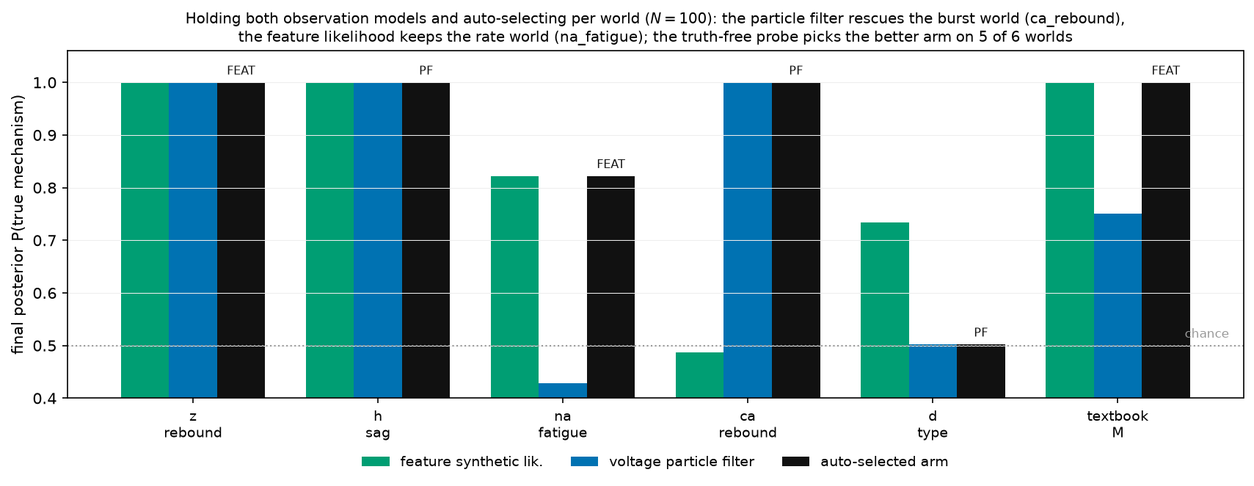
The learned summary and the spot-check in the open-world loop.

The two-hypothesis study above pits the particle filter against a fixed-feature synthetic likelihood. The released open-world benchmark adds a third, still cheaper option — a synthetic likelihood on a learned summary $s_\phi$ (a frozen $1$ d CNN, Appendix A.4) — so the cost-aware selection of Equation 12 now ranges over $o\in{\text{PF}, \ \text{feat}, \ s_\phi}$, guarded by the particle-filter spot-check of Appendix A. Running the full $\mathcal{M}$-open battery (six worlds, three seeds, the LLM proposing its own candidate channels at $N_{\text{noise}}{=}100$; Figure 33), the cost-aware probe selects a cheap model on every run, and the spot-check overrides it to the PF wherever the cheap posterior disagrees with the filter. Of the $18$ runs the final observation model was the learned $s_\phi$ on $2$, the fixed feature likelihood on $5$, and the particle filter on $11$ — all $11$ reached via a spot-check disagreement. So the frozen $s_\phi$ is used only where it is verifiably sufficient (its posterior matches the filter's, e.g. $\textsc{h-sag}$ and $\textsc{d-type}$), while the PF anchor catches the confusable cases. The sharpest is $\textsc{ca-rebound}$: the cheap summaries confidently prefer a slow-Na$^+$ run-down, but the filter — and the T-type Ca current the LLM proposed — win, cutting its feature-forecast error from $4.5$ (feature-only) to $0.85$, with mean mechanism recovery $0.94$ across the battery ($19$ LLM calls, $0.55$ total). Figure 31 visualises one such disagreement on $\textsc{d-type}$.

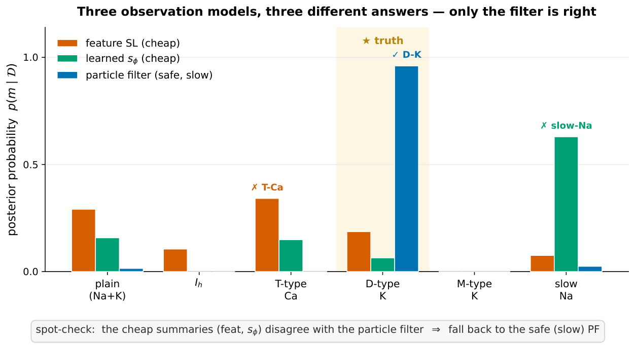
F.4 Data efficency experiments

The data efficiency curves from applying MDA and baseline LLM to $\textsc{NeuronBenchStoch}$ are shown in Figure 32. We see that MDA is substantially more data efficient. In Figure 33 we show the final error for each world after $B=6$ experiments, as a fraction of each world's no-experiment ($N_a{=}0$) prior (the raw MSEs are not comparable across worlds — they span an order of magnitude through the priors alone, so textbook_M's large absolute error is a distant prior, not a hard world). Normalised this way, the exploitable worlds (textbook_M, $\textsc{ca-rebound}$) collapse to ${\sim}5%$ of prior, while the noise-dominated $\textsc{z-rebound}$ and $\textsc{d-type}$ hover near the prior. The top row shows the spike forecast MSE and the bottom row the feature forecasts. The 3 dots represent the 3 trials per world; we color code them by the observation model that was chosen by the agent. The learned summary was chosen 1/3 times for $\textsc{h-sag}$ and 1/3 times for $\textsc{d-type}$; the fixed (feature) summary was chosen 2/3 times for $\textsc{na-fatigue}$; the rest of the time the agent chose particle filtering, which is the safest choice.

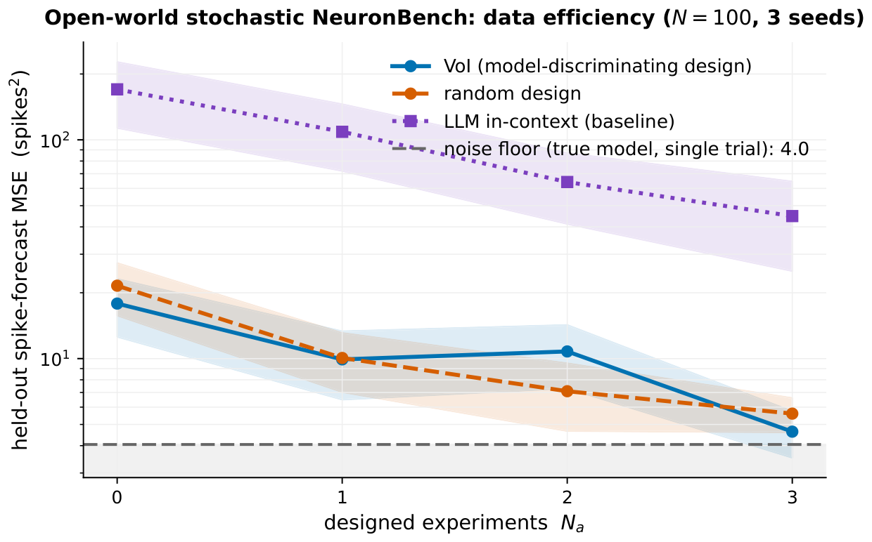
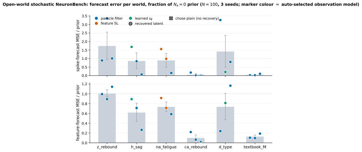
F.5 Wiring the repeat count into the VoI design space

When the data is noisy, it is useful to be able to repeat experiments, to average the noise down. We therefore enlarge the design to $\xi=(\text{protocol}, \ r)$, where $r$ is a repeat count costing $r$ units of budget: averaging $r$ repeated trials shrinks the spike-count noise ${\sim}1/\sqrt{r}$, so re-running the informative protocol is itself a design lever the agent can pull.

Expanded VoI.

The expanded VoI equation becomes

$ \xi^\star ;=; \arg\max_{\xi}\ \frac{\mathrm{MI}\big(m;\ \bar{s}_r(y)\mid \xi\big)} {\mathrm{cost}(\xi)},\tag{26} $

where $\bar{s}r(y)=\tfrac1r\sum{t=1}^r s\big(y^{(t)}\big)$ is the feature vector averaged over the $r$ trials, and $\mathrm{cost}(\xi)=r$ is the number of repeats. Here the per-trace summary $s(y)$ is the six stochastic-battery features in Equation 22.

Concretely, let $w_m=p(m\mid \mathcal{D})$ be the current posterior over the candidate mechanisms. The $r$-averaged features have the (simulation-estimated) Gaussian synthetic likelihood $p(\bar{s}r\mid m, \xi)= \mathcal{N}!\big(\bar{s}r\mid \mu{m, \xi}, , \tfrac1r\Sigma{m, \xi}\big)$, with $\mu_{m, \xi}, \Sigma_{m, \xi}$ read off $R$ simulated traces per candidate, where $\Sigma$ is diagonal when using the summary vector in Equation 5. (The $\tfrac1r$ factor being the variance reduction from averaging.) The information gain is the expected drop in the entropy of the model posterior, similar to 12:

$ \mathrm{MI}\big(m;\bar{s}r\mid \xi\big)=H(w)-\mathbb{E}{p(\bar{s}_r\mid \xi)}!\big[H\big(q(\cdot\mid\bar{s}_r)\big)\big], \qquad q(m\mid\bar{s}r)=\frac{w_m, p(\bar{s}r\mid m, \xi)}{\sum{m'}w{m'}, p(\bar{s}_r\mid m', \xi)},\tag{27} $

with prior entropy $H(w)=-\sum_m w_m\log w_m$ and posterior-predictive feature mixture $p(\bar{s}r\mid \xi)=\sum_m w_m, \mathcal{N}!\big(\bar{s}r\mid\mu{m, \xi}, \tfrac1r\Sigma{m, \xi}\big)$. We evaluate Equation 27 by Monte Carlo over that mixture: draw $J$ samples $m^{(j)}!\sim w$, $\bar{s}r^{(j)}!\sim \mathcal{N}!\big(\mu{m^{(j)}}, \tfrac1r\Sigma_{m^{(j)}}\big)$, form each model posterior $q(\cdot\mid\bar{s}_r^{(j)})$, and average the per-sample gain $H(w)-H\big(q(\cdot\mid\bar{s}_r^{(j)})\big)$ over the $J$ draws ($J{=}200$ here). Because averaging shrinks the noise, VoI can now spend budget re-running the discriminator to beat the channel noise, rather than being forced onto uninformative decoy protocols. This is the VoI objective of Equation 9 with the repeat count promoted to a first-class part of the design.

Results.

As a proof of concept, we run the whole six-world battery (using a fixed set of hypotheses) across the full channel-count ladder — from near-deterministic ($N_{\text{noise}}{=}3000$) to strongly stochastic ($N_{\text{noise}}{=}50$) — using the synthetic factored Gaussian likelihood with the fixed summary features from Equation 22. In Figure 34 we plot the mean posterior on the truth over the six worlds. All acquisition policies degrade gracefully with noise, from certainty at $N_{\text{noise}}{=}3000$ to $0.8$ – $0.9$ at $N_{\text{noise}}{=}50$. Repeat-aware VoI leads at every rung, and — the key point — its margin widens as the noise grows: from a tie at $N_{\text{noise}}{\ge}1000$ to $0.91$ vs. $0.80$ over each-once/random at $N_{\text{noise}}{=}50$. Spending budget on repeats is exactly the lever that matters most when the per-experiment signal is weakest.

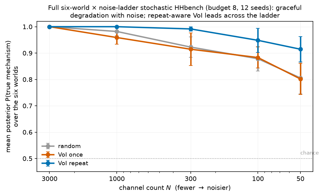
G. Further related work

Here we expand on connections to prior work that we did not have space for in Section 5. Specifically we discuss conceptual relationship to predictive knowledge representations (general value functions), generative world models in RL, simulation-based inference, and self-supervised representation learning (JEPA). The unifying thread is the distinction, central to our method, between the raw observation $y_{1:T}$, the summary $s(y)$ that inference conditions on, and the fixed target functional $F_q(y)$ that the task scores (Appendix A.1).

General value functions and cumulants.

The general value function (GVF) framework ([58, 59, 60, 61]) represents an agent's knowledge as a large collection of predictive questions, each a value function of a scalar cumulant (pseudo-reward) $c(s)$ accumulated under a policy $\pi(a|s)$ and a (possibly state-dependent) discount $\gamma$:

$ V(s;\pi, \gamma, c) = E_{\pi \times p^*} \left[\sum_{t=1}^{\infty} \gamma^t c(s_{t}) \mid s_0=s \right]\tag{28} $

where $p^*(s'|s, a)$ is the (unknown) environment model. Our target functional $F_q(y)$ plays the role of the GVF cumulant, and our query distribution $\mathcal{Q}$ is, like a set of GVFs, a bank of predictive questions that operationally defines what the model must be "useful" for. The differences are what make our setting a discovery, rather than a control, problem:

• Non-Markovian trajectory functional, not an online cumulant. A GVF accumulates a Markov, per-step cumulant $c_t$; our target $F_q(y_{1:T})$ is an arbitrary functional of the whole observed trajectory (e.g. the test-window spike count, or a per-probe trajectory RMS), computed after the rollout rather than bootstrapped online.
• No discounting or return. GVFs predict a discounted return $\mathbb{E}[\sum_t \gamma^t c_t]$; we predict $F_q$ directly, undiscounted, over a finite horizon that is fixed by the query design $\xi$ rather than by a temporal-credit-assignment discount.
• Open-loop designs, not closed-loop policies. A GVF conditions on a behaviour policy $\pi$ mapping states to actions (closed-loop, reactive). Our "policy" is an open-loop experiment design $\xi=(\iota, a, x_{1:T})$ — an initial condition, an intervention, and an input sequence chosen before the rollout — i.e. an experimental protocol, not a controller. Consequently $\mathcal{Q}$ is a distribution over designs/protocols, and the inner objective is experiment design (VoI, Appendix A.2), which has no analogue in the standard GVF setting where the policy is given.

In short, $F_q$ generalises the scalar reward of value-equivalent models ([62]) to an arbitrary, non-Markovian trajectory functional, and the class of mechanisms that agree on $\mathcal{Q}$ is our analogue of a value-equivalence class — but reached by designed interventions and open-ended mechanism search, not by learning a policy with temporal difference methods.

Generative world models in RL: Dreamer and MuZero.

Two poles bracket our summary $s(y)$. Dreamer ([63]) learns a generative latent world model trained to reconstruct observations; the training signal is dense, but capacity is spent modelling nuisance detail (all the pixels) that is irrelevant to any downstream decision. MuZero and the value-equivalence principle ([64, 62]) go to the other extreme: they model only what affects value, so the model is decision-aligned but the reward signal is sparse and the model is badly under-determined off the behaviour distribution. MDA occupies the middle: a summary $s(y)$ that is richer than a scalar reward — hence a dense training signal, as in Dreamer — yet projected onto the task via the fixed target $F_q$ and query bank $\mathcal{Q}$ — hence decision-aligned, as in MuZero. Unlike either, the model is an explicit mechanistic hypothesis (interpretable, and sound under interventions it never saw, per [4, 65]), inferred Bayesianly under a hard experiment budget.

Simulation-based inference and learned summaries.

Our inference is a form of simulation-based inference (SBI) ([38]): for intractable likelihoods we replace $p(y_{1:T}\mid m, \theta)$ with a synthetic likelihood $p(s(y)\mid m, \theta)$ in summary space ([49, 28]). The motivation for summaries — discard nuisance variation the parameters do not control — is, almost word for word, the self-supervised-learning argument for predicting in representation space rather than pixel space (see discussion of JEPA below). The crucial lesson SBI has already internalised is that a learned summary must be anchored to an external referent to avoid collapse (where $s(y)$ is a constant, thus incurring no predictive loss but also providing no information from the data): Fearnhead–Prangle ([39]) regress the summary onto $\theta$, and neural-sufficient-statistic methods ([40]) maximise $I(\theta; s_\phi(y))$. Our learned encoder $s_{\phi}$ (Appendix A.4) is trained the SBI way — a supervised head that recovers $(m, \theta)$. This makes it $s(y)$ sufficient to distinguish the different $m \in \mathcal{M}$, but if we grow the hypothesis space $\mathcal{M}$, we may also need to update $s(y)$: we detect this by using an out-of-sample $\textsc{query}$ check (see the anti-collapse discussion below for details).

JEPA and representational collapse.

Given an $(x, y)$ pair, Joint-embedding predictive architectures ([66, 67]) predict a target embedding from a context embedding:

$ s_x = f_{\text{ctx}}(x), \quad s_y = f_{\text{tgt}}(y), \quad \hat{s}_y = g(s_x, z) $

where $z$ is an auxiliary hidden variable to explain any residual not predictable from the input. The predictor $g$ and encoders $f$ are trained to minimize

$ \mathcal{L}_{\text{JEPA}} = E\left[|| \hat{s}_y - \text{stopgrad}(s_y) ||^2 \right] $

Crucially the model is trained without a generative loss, which avoids the problem of pixel reconstruction/prediction. This is structurally the same move as SBI summaries. But with no external parameter to anchor against, the encoders can collapse to a constant (the loss is zero, the representation worthless). The standard fixes are architectural: stop-gradient/EMA on the prediction targets; variance–covariance (VICReg) penalty, which explicitly require each embedding dimension to have nonzero variance and dimensions to be decorrelated; or, in LeJEPA's SIGReg method ([68]), push the aggregated embedding distribution to $\mathcal{N}(0, I)$ using a sliced kernel discrepancy (MMD) metric.

Var-JEPA ([69]) makes the correspondence with SBI explicit: the JEPA predictor is a Gaussian synthetic likelihood / learned conditional prior, and collapse is averted precisely when reconstruction terms turn the objective into a genuine likelihood bound (ELBO). MDA needs none of these stop-gradient hacks, for the reason SBI never hits collapse: it has a simulator. The simulator is the free "reconstruction anchor" that JEPA fakes, and, unlike a JEPA trained on a fixed dataset, MDA can query the simulator at new designs, which is what lets it (i) train $s_{\phi}$ on the prior-predictive mechanism family and (ii) actively design the maximally-disagreeing experiment that excites any dimension a collapsed summary would ignore. The disanalogy is the same one that makes collapse possible in the first place: JEPA's "parameter" $s_x$ is invented by the optimiser that also fits the predictor, so an optimiser free to choose both question and answer picks an easy one; our parameters $m, \theta$ and target $F_q$ are fixed by the scientific problem.

Generalised Bayes and scoring rules.

Our synthetic-likelihood update is ordinary Bayes in summary space, and inherits its efficiency when the Gaussian-summary model Equation (11) is roughly correct but also its brittleness under misspecification. A principled alternative for the stochastic regime is a generalised-Bayes (Gibbs) posterior ([70]) built from a proper kernel or energy scoring rule ([71, 72]): it is computed from simulator draws alone (no density), and is provably robust (bounded influence) to model error, at the cost of statistical efficiency and a free learning rate that must be calibrated. Swapping the synthetic likelihood for a scoring-rule posterior — leaving the LLM proposal, VoI design, and $\mathcal M$-open expansion untouched — is a natural extension when the Gaussian-summary assumption is unsafe.

H. LLM prompts

This appendix reproduces the prompts used by the three domains of this paper (physics, chemistry, biology). Throughout, the LLM runs at temperature $0.2$ – $0.4$ with JSON-mode responses and every call is cached for reproducibility; the base model is stated per experiment (Opus 4.7 unless noted, with the base-model robustness sweep of Appendix C.8 using Fable 5 and DeepSeek v4, and the $\textsc{ChemBench}$ head-to-head using a matched proposer). MDA uses the LLM only to propose structures and, in the baseline arms, to acquire experiments and forecast; inference, VoI design, and fitting are exact Bayesian computations.

H.1 ForceBench (force laws, § 4.1)

The physics rung invokes the LLM in four distinct roles, which fall into two groups: the proposer, which is the only LLM call inside MDA's discovery loop, and the verbaliser/judge, which are the benchmark's own explanation-scoring machinery and play no part in discovery, inference, or forecasting.

H.1.1 MDA proposer (the only LLM call in the discovery loop)

The proposer sees the world context, the probe data collected so far, and a language specification that steers it toward field-equation Green's functions rather than curve-fits; it returns candidate force laws as JSON (parsed, compiled, and SMC-fit by MDA). Note that the language spec names screened/power-law/oscillatory families (including the $K_1$ Yukawa form) as examples, so the proposer is given the physical vocabulary — MDA's contribution is the inference and VoI design that identify which form the data support (see App. Appendix C, Figure 15), not blind form-discovery. Its system message and user template:

SYSTEM:
You are a physicist proposing candidate pairwise force laws to explain probe-orbit data. Reply JSON only.

USER (world context, then the observed data, then the language spec):

A test probe moves in an unknown central force sourced by a fixed body at the origin. The force MAY be static or MAY vary with time t (e.g. a time-modulated coupling). Each experiment launches the probe from a position with a velocity, and sets two knobs p1, p2. <one sentence naming the two experiment knobs p1, p2 for this world -- e.g. p1 the source coupling, p2 the probe inertia> F_mag is the pairwise force magnitude between the probe (charge qi) and source (charge qj) at separation r and time t.

Observed data:
<measurement times and the radius r(t) of each probe run so far>

Propose N distinct plausible force laws (or refinements of those tried).

Propose each force law as the field / Green's-function response of a PHYSICAL FIELD EQUATION (e.g. 2D Laplacian/Poisson -> 1/r; screened Poisson / Helmholtz -> a screened form such as exp(-r/lam)/r or K1(r/lam)/lam; fractional Laplacian -> a power law 1/r^p; 3D inverse-square -> 1/r^2), NOT an arbitrary curve-fit with softening/offset terms. If the data show the force changing sign or magnitude over time (not just with r), the coupling itself may be time-dependent (e.g. a cos(w*t+phi) modulation) -- consider such forms too. State the governing operator in the rationale. Express each F_mag as a Python expression in the symbols r, qi, qj, t and your OWN named free parameters ONLY. The source coupling is carried by qj (the probe is qi); do NOT reference p1 or p2 in the expression -- introduce named parameters (e.g. k, G, lam, s) for coupling constants and length scales. Allowed functions: exp, log, sqrt, sin, cos, tanh, k0, k1, gamma, pi, np. Return JSON {"hypotheses": [{"name": str, "fmag": str, "operator": str, "params": [{"name": str, "low": float, "high": float}], "rationale": str}]}.

For the extension worlds (App. Appendix C) only the proposer context changes — the declared background field (ether/Hubble), the self-interacting cloud (circle), or the known-law hidden sources (dark matter); the language spec is unchanged:

ETHER / HUBBLE (central force + declared background):

Here the probe is a neutral test particle (qi=1) orbiting a fixed central anchor that sources the field (coupling carried by a named parameter); its inertia is 1.
Test probes orbit an unknown CENTRAL force sourced by a fixed anchor at the origin (a 2D field-equation response, e.g. a Laplacian giving F ~ 1/r). <probe roles> LAYERED ON TOP there is a uniform, mass-independent background acceleration of magnitude alpha in the +y direction (a constant 'ether' drift), on top of the central force. That background is handled separately by the fitter -- you only need to propose the CENTRAL pairwise force magnitude F_mag(r, qi, qj, t) sourced by the anchor. F_mag is the magnitude of the attractive central force on the probe at separation r from the anchor.

----------------------------------------
CIRCLE (self-interacting N-body):

Eleven identical particles -- one at the centre and ten equally spaced on a ring -- ALL interact with each other through the SAME pairwise central force (uniform coupling): every particle both sources the field and feels it. Each experiment sets the ring radius and a tangential launch velocity. Propose the pairwise force magnitude F_mag(r, qi, qj, t) between any two particles at separation r (with qi=qj=1, the uniform coupling); it is attractive and depends only on r for a static field. The many-body motion is the sum of these pairwise forces.

----------------------------------------
DARK MATTER (known law, latent hidden sources):

Test probes move in a KNOWN static 2D-Laplacian field (each source contributes F = q/(2*pi*r), attractive), sourced by 20 VISIBLE particles of coupling 1 whose positions are known, PLUS an unknown number of HIDDEN sources that reveal themselves only through the probes' deflection toward seemingly empty regions. The task is to infer how many hidden sources exist and their positions and couplings.

(three species uses no LLM proposer -- the couplings are inferred by a linear solve; the LLM only verbalizes the recovered species, via the verbaliser above.)

H.1.2 Verbaliser and judge (benchmark explanation scoring; not used for discovery)

These two roles exist only to compute the benchmark's explanation metric: the verbaliser turns MDA's already-selected law into a short prose explanation, which the benchmark's own judge scores against the world's optimal explanation and rubric (temperature $0$, integer $0$ – $10$). MDA's posterior, VoI design, and held-out forecasts never call either.

SYSTEM:
You are a physicist. Reply with a 2-4 sentence explanation only.

USER:

<world context>

A Bayesian model-discovery method fit the data and selected the force law F_mag = <the fitted F_mag expression> with FITTED parameters {'<parameter names>': np.float64(0.0)}. Explain the physics of THIS law, and be specific and complete: (1) name the governing field equation / operator; (2) state its temporal character (static vs time-evolving); (3) give the NUMERIC value of any length- or scale-parameter you fitted (e.g. a screening length) and say how the force behaves at short vs long range; (4) explicitly state the physical roles of the knobs p1 and p2 as described above.

SYSTEM:
You are an expert physicist grading how well a student's prose description of a simulated physical system matches the ground-truth description. You are precise, fair, and reward semantic correctness over surface phrasing -- paraphrases and equivalent formulations (e.g. 'inverse-square-like' ~= 'grad^2phi' in 2D) should receive credit, but missing or wrong physical content should not.

USER TEMPLATE:

Compare the student's description against the ground-truth description of the physical system.

<ground_truth>
{ground_truth}
</ground_truth>

<student>
{student}
</student>

Score the student description on a 0-10 integer scale based on how well it captures:
  1. The correct field equation / governing operator (e.g. Laplacian, fractional Laplacian, Helmholtz, diffusion, wave).
  2. The temporal character (static vs. time-evolving; instantaneous vs. retarded).
  3. The force law / coupling structure (how particles couple to the field, including p1/p2 roles).
  4. Any structural features unique to this world: hidden species and their relative coupling strengths and signs, neutral probes, hidden/dark sources, screening lengths, etc.

Use the world-specific rubric below to calibrate the bands. A 10/10 represents the best explanation achievable given the experimental capabilities -- reward semantically-equivalent phrasings and numeric estimates within the tolerance specified by the rubric.

<scoring_rubric>
{rubric}
</scoring_rubric>

Respond with 1-3 sentences of justification, then your final integer score inside <score>...</score> tags. Example: "<score>7</score>".

H.1.3 Baseline forecasters

(The $N_a{=}0$ and LLM-forecast arms of Figure 2.) The zero-shot baseline reuses the proposer's system prompt and world context but appends, in place of any data, the instruction: "No experimental budget is available: you cannot run any experiments or fits. Based ONLY on physical reasoning about the setup described above, submit your single best-guess law now" (a <final_law> discovered_law(...) plus an <explanation>). The LLM-forecast baseline is the same, but with the collected experiments' launch configurations and observed radii $r(t)$ listed before the submission instruction — so the LLM authors a law from the data in context (rather than MDA templating one from its posterior), scored by the benchmark's own executor exactly as MDA's Bayes-forecast is.

H.2 ChemBench (enzyme rate laws, § 4.2)

As in physics, the only LLM call inside MDA's discovery loop is the proposer. It sees an enzyme-kinetics mechanism grammar, the experiments collected so far (design inputs $\to$ observed initial rate $r_0$), and — when refining an existing pool — the forms already tried together with their residuals (so it does not re-propose dead ends, and knows which input a residual correlates with, e.g.\ a residual growing with temperature suggests an Arrhenius factor) plus the remaining budget and phase. It returns candidate rate laws as JSON, which MDA compiles and SMC-fits; inference, VoI design, and fitting are exact Bayesian computations. The grammar names the standard families (Michaelis–Menten, Hill, competitive/uncompetitive/noncompetitive inhibition, product inhibition, Arrhenius temperature, ping-pong) as the physical vocabulary, so — exactly as in physics — MDA's contribution is identifying which multiplicative composition the data support, not blind symbol search. The residual-directed context engineering (negative evidence $+$ budget/phase) follows LLM-AutoSciLab ([2]). System message and user template:

SYSTEM:
You are an enzyme kineticist proposing candidate rate laws to explain assay data. Reply JSON only.

USER (world context + mechanism grammar, then the observed data, then -- only when refining -- residual-directed negative evidence and the remaining budget/phase, then the language spec):

An enzyme catalyses a reaction with initial rate r0 [mM/min]. Controllable inputs: C_A [substrate, mM], C_I [inhibitor, mM], C_B [2nd substrate, mM], C_P [product, mM], Enz [enzyme, mg/mL], T [K], pH. Discover r0 = f(C_A,C_I,C_B,C_P,Enz,T,pH; theta).
Mechanism families to consider (identify which are active FROM THE DATA):
  Substrate C_A: linear | Michaelis-Menten C_A/(Km+C_A) | Hill C_A**n/(Kh**n+C_A**n) | substrate inhibition C_A/(Km+C_A+C_A**2/Ki)
  Inhibitor C_I: none | competitive (raises apparent Km) | uncompetitive (lowers Vmax) | noncompetitive (lowers Vmax at all C_A)
  Product C_P: none | product inhibition (like competitive but in C_P)
  Temperature T: none | Arrhenius exp(-Ea/8.314*(1/T-1/310))
  Second substrate C_B: none | ping-pong C_A*C_B/(KmA*C_B+KmB*C_A+C_A*C_B)
  Enzyme Enz: rate is proportional to Enz (Vmax = kcat*Enz).
Compose factors multiplicatively when several mechanisms act together.

Experiments (inputs -> r0):
  <one line per collected experiment: C_A=.., C_I=.., C_B=.., C_P=.., Enz=.., T=.., pH=.. -> r0=..>

[when refining an existing pool -- residual-directed negative evidence:]
Forms ALREADY TRIED (in the pool) and their residuals -- do NOT re-propose any of these; propose forms STRUCTURALLY DIFFERENT from all of them:
  <per-form median relative residual; and, for the current best form, which input its residual correlates with -- e.g. residual grows with T -> add Arrhenius; with C_I -> add an inhibitor term>
Refine by proposing a DIFFERENT mechanism combination (add/remove an inhibition, Hill, Arrhenius, or ping-pong factor) -- do NOT patch with ad-hoc offset/softening terms.

[budget/phase status, when set:]
Experiment budget remaining: <B>. Current phase: <explore|refine> (explore = restructure the mechanism; refine = tune an adequate form).

Propose N distinct plausible rate laws (or refinements of those tried).
Each 'expr' is a Python expression in the 7 input names + your declared params, using only + - * / ** and exp, log, sqrt. Give physically plausible positive param bounds. JSON schema: {"hypotheses":[{"name":str,"expr":str,"params":[{"name":str,"low":float,"high":float}]}]}

The head-to-head baseline (Appendix D) is the $\textsc{LLM-AutoSciLab}$ agent's own LLM $+$ active-learning $+$ symbolic-regression loop ([2]), run under matched settings (the same LLM, budget, noise, and universal grammar); its prompts are those of that system and are not reproduced here.

H.3 Electrophysiology (ion channels, § 4.3)

We group the $\textsc{NeuronBench}$ prompts by their role. The model-proposal prompt is the only LLM call inside MDA's discovery loop: MDA uses the LLM to propose candidate mechanisms, then fits and selects them by exact SMC and designs experiments by numerical VoI — so this is the prompt MDA's results depend on. The baseline prompts (experiment design and forecasting) are used only by the LLM baseline arms MDA is compared against, never by MDA itself. All are zero-reference: the LLM is told only to model the cell as a conductance-based neuron and infer its channels from the data — never the candidate models, the posterior, or the true mechanism.

What the LLM sees as "data".

An experiment yields a membrane-voltage trace $V(t)$, but every LLM prompt is shown only its reduction to the test-window spike count — one line per protocol run, formatted verbatim as:

Experiments run so far and observed spike counts:
- long step (10 uA, 300 ms) -> 21 spikes
- paired long pulses (12/300, 60 gap, 12/300) -> 16 spikes
- hyperpol step then release (-30/250 -> rebound) -> 4 spikes

The raw trace $V(t)$ is never sent to any LLM. It is available only to MDA's numerical observation model (Appendix F.3), which chooses whether to reduce it to a spike count or score it directly with a particle filter — the reduction-vs-model choice is the solver's, not the benchmark's.

H.3.1 MDA model proposer (the only LLM call in MDA's loop)

In the released open-world benchmark the proposer returns its own parameterised channel hypotheses (reversal potential, activation direction, inactivation, and conductance / half-activation / time-constant bounds), so the hypothesis space is genuinely open:

System: You are an electrophysiologist proposing candidate ion-channel mechanisms to explain
        current-clamp spike-count data. Reply with a JSON object only.
User:   A neuron is recorded in current clamp and fires action potentials under injected current.
        Model it as a single-compartment conductance-based (Hodgkin-Huxley) neuron with voltage-gated
        channels. From the spike-count data, propose candidate membrane currents (beyond the standard
        Na+/K+ spiking currents) that could explain its responses. Each is described by:
          reversal_mV : reversal potential (~+50 Na-like, ~+120 Ca-like, ~-80 K-like, ~-30 mixed)
          opens_on    : 'depol' or 'hyperpol'
          inactivates : true if transient / de-inactivated by a hyperpolarising pre-pulse
          bounds for conductance g, half-activation voltage (mV), and activation time constant (ms).
        <collected protocol -> spike-count data>
        Propose N distinct plausible mechanisms (or an empty list if the data look like a plain spiker).
        JSON schema: {"hypotheses":[{"name","reversal_mV","opens_on","inactivates",
                      "g_bounds","half_mV_bounds","tau_ms_bounds"}]}

The $\textsc{h-sag}$ deep-dive example (Figure 24) instead asks for candidate channel compositions from a channel menu, given a one-line phenotype description:

A neuron recorded in current clamp rests near -65 mV and fires overshooting action
potentials to a supra-threshold current step. Model it as a single-compartment
conductance model with voltage-gated channels from {Na (fast, TTX-sensitive), K
(delayed rectifier), Ca (high-threshold), leak}. Propose 4-5 DISTINCT candidate
channel COMPOSITIONS that could underlie the spiking (plus at least one non-spiking
null), each a list from {Na,K,Ca,L}. Return exactly {"compositions": [{"name": "...",
"channels": ["Na","K","L"]}, ...]}.

H.3.2 LLM baselines: experiment design and forecasting (not used by MDA)

As an experiment proposer (the LLM-acquisition baseline) the LLM chooses the next protocol from the collected data alone:

System: You are an electrophysiologist choosing the next experiment. Reply with ONLY a JSON object.
User:   A neuron is recorded in current clamp; we count its action potentials per protocol. Model it
        as a single-compartment conductance-based (Hodgkin-Huxley) neuron with voltage-gated channels
        (Na, K, Ca, leak, and possibly others), and infer its mechanism from the data.
        Experiments run so far and observed spike counts:
          - <protocol> -> <count> spikes ...
        Available experiments (choose one; each may be run once):
          - <protocol label> ...
        Which ONE experiment best reveals the neuron's mechanism next?
        Return exactly {"experiment": "<one label copied verbatim>"}.

As the ICL-forecaster (the in-context-learning baseline) it predicts the held-out spike counts:

System: You are an electrophysiologist forecasting a neuron's response. Reply with ONLY a JSON object.
User:   A neuron is recorded in current clamp; we count its action potentials (spikes) per protocol.
        Model it as a single-compartment conductance-based (Hodgkin-Huxley) neuron with voltage-gated
        channels (Na, K, Ca, leak, and possibly others).
        Experiments run and observed spike counts:
          - <protocol> -> <count> spikes ...
        Predict the spike count for each held-out protocol:
          1. <protocol> ...
        Return exactly {"counts": [n1, ...]} with one integer per protocol, in order.

The $N_a{=}0$ (zero-shot) neuron point is this forecaster with an empty "experiments run" list. These prompt templates mirror the code (scripts/ephys/hh_worlds_run.py and the released neuronbench), so the documented prompt is the one that is run.

References

Section Summary: The references compile recent research papers, books, and preprints exploring how artificial intelligence and large language models can support scientific discovery, experimentation, and reasoning. Many focus on causality, Bayesian experimental design, and the gap between predictive power and genuine understanding in automated systems. They draw on both classic works in statistics and philosophy as well as cutting-edge studies from 2024–2026.

[1] Matt L. Wiemann, Lindsay M. Smith, Peter Melchior, Siddharth Mishra-Sharma, Andrew Gordon Wilson, Pavel Izmailov, and Carolina Cuesta-Lázaro. DiscoverPhysics: Benchmarking LLMs for out-of-the-box scientific thinking. arXiv preprint arXiv:2605.26087, 2026.

[2] Sanchit Kabra, Nikhil Abhyankar, Saaketh Desai, Prasad Iyer, and Chandan K. Reddy. Llm-autoscilab: Closed-loop scientific discovery via active experimentation with llms. arXiv:2605.24043, 2026.

[3] Judea Pearl. Causality: Models, Reasoning, and Inference. Cambridge University Press, 2nd edition, 2009.

[4] Jonathan Richens and Tom Everitt. Robust agents learn causal world models. In International Conference on Learning Representations (ICLR), 2024. URL https://openreview.net/forum?id=pOoKI3ouv1. Oral; honorable mention outstanding paper. arXiv:2402.10877.

[5] Wesley C Salmon. Scientific explanation and the causal structure of the world. Princeton University Press, Princeton, NJ, December 1984. URL https://press.princeton.edu/books/paperback/9780691101705/scientific-explanation-and-the-causal-structure-of-the-world.

[6] Mario Krenn, Robert Pollice, Si Yue Guo, Matteo Aldeghi, Alba Cervera-Lierta, Pascal Friederich, Gabriel Dos Passos Gomes, Florian Häse, Adrian Jinich, Akshatkumar Nigam, Zhenpeng Yao, and Alán Aspuru-Guzik. On scientific understanding with artificial intelligence. Nat. Rev. Phys., 4(12):761–769, October 2022. URL https://pmc.ncbi.nlm.nih.gov/articles/PMC9552145/.

[7] Lisa Messeri and M J Crockett. Artificial intelligence and illusions of understanding in scientific research. Nature, 627(8002):49–58, March 2024. URL https://www.nature.com/articles/s41586-024-07146-0.

[8] Jürgen Bajorath. From scientific theory to duality of predictive artificial intelligence models. Cell Rep. Phys. Sci., 6(4):102516, April 2025. URL https://www.sciencedirect.com/science/article/pii/S2666386425001158.

[9] Thomas Serre and Ellie Pavlick. From prediction to understanding: Will AI foundation models transform brain science? Neuron, 2025. URL http://dx.doi.org/10.48550/arXiv.2509.17280.

[10] Stefan Kramer, Mattia Cerrato, Jannis Brugger, Sašo Džeroski, and Ross D King. Automated scientific discovery: From equation discovery to autonomous discovery systems. Mach. Learn., 115(5):109, May 2026. URL https://link.springer.com/article/10.1007/s10994-025-06955-2.

[11] Elias Bareinboim, Juan D Correa, Duligur Ibeling, and Thomas Icard. On pearl’s hierarchy and the foundations of causal inference. In Probabilistic and Causal Inference: The Works of Judea Pearl, volume 36, pp. 507–556. Association for Computing Machinery, New York, NY, USA, 1 edition, March 2022. URL https://causalai.net/r60.pdf.

[12] A Philip Dawid. Statistical causality from a Decision-Theoretic perspective. Annu. Rev. Stat. Appl., 2(1):273–303, 2015. URL https://doi.org/10.1146/annurev-statistics-010814-020105.

[13] P. Dawid. Causal inference without counterfactuals. JASA, 95:407–448, 2000.

[14] D. V. Lindley. On a measure of the information provided by an experiment. The Annals of Mathematical Statistics, 27(4):986–1005, 1956. doi:10.1214/aoms/1177728069.

[15] Kathryn Chaloner and Isabella Verdinelli. Bayesian experimental design: A review. Statistical Science, 10(3):273–304, 1995.

[16] Tom Rainforth, Adam Foster, Desi R. Ivanova, and Freddie Bickford Smith. Modern Bayesian experimental design. Statistical Science, 39(1), 2024.

[17] Emre Kıcıman, Robert Ness, Amit Sharma, and Chenhao Tan. Causal reasoning and large language models: Opening a new frontier for causality. Transactions on Machine Learning Research, 2024. ISSN 2835-8856. URL https://openreview.net/forum?id=mqoxLkX210. Featured Certification. Preprint: arXiv:2305.00050.

[18] José M. Bernardo and Adrian F. M. Smith. Bayesian Theory. Wiley, 1994.

[19] Riko Kelter. Bayesian model selection in the $\mathcal{M}$-open setting — approximate posterior inference and subsampling for efficient large-scale leave-one-out cross-validation via the difference estimator. arXiv preprint arXiv:2005.13199, 2020.

[20] Markus J Buehler. Why we must break the world. ChemRxiv, May 2026. URL https://chemrxiv.org/doi/pdf/10.26434/chemrxiv.15001674/v2.

[21] Noémi Elteto, Nathaniel D Daw, Kimberly L Stachenfeld, and Kevin J Miller. ATLAS: Active theory learning for automated science. arXiv [cs.LG], June 2026. URL http://dx.doi.org/10.48550/arXiv.2606.12386.

[22] Silviu-Marian Udrescu and Max Tegmark. AI feynman: A physics-inspired method for symbolic regression. Science Advances, 6(16):eaay2631, 2020.

[23] Stefan Wahl, Raphaela Schenk, Ali Farnoud, Jakob H. Macke, and Daniel Gedon. A probabilistic framework for LLM-based model discovery. arXiv preprint arXiv:2602.18266, 2026. URL https://arxiv.org/abs/2602.18266. Introduces ModelSMC.

[24] Wasu Top Piriyakulkij, Cassidy Langenfeld, Tuan Anh Le, and Kevin Ellis. Doing experiments and revising rules with natural language and probabilistic reasoning. In Advances in Neural Information Processing Systems (NeurIPS), 2024.

[25] Christian A Naesseth, Fredrik Lindsten, and Thomas B Schön. Elements of sequential monte carlo. Foundations and Trends in Machine Learning, 2019. URL http://arxiv.org/abs/1903.04797.

[26] Nicolas Chopin and Omiros Papaspiliopoulos. An Introduction to Sequential Monte Carlo. Springer, 1 edition, October 2020. URL https://nchopin.github.io/books.html.

[27] D MacKay. Bayesian model comparison and backprop nets. In NIPS, pp. 839–846, December 1991. URL https://proceedings.neurips.cc/paper/1991/file/c3c59e5f8b3e9753913f4d435b53c308-Paper.pdf.

[28] Michael Deistler, Jan Boelts, Peter Steinbach, Guy Moss, Thomas Moreau, Manuel Gloeckler, Pedro L C Rodrigues, Julia Linhart, Janne K Lappalainen, Benjamin Kurt Miller, Pedro J Gonçalves, Jan-Matthis Lueckmann, Cornelius Schröder, and Jakob H Macke. Simulation-based inference: A practical guide. arXiv [stat.ML], August 2025. URL http://dx.doi.org/10.48550/arXiv.2508.12939.

[29] Tom Zahavy. Position: LLMs can't jump. In ICML, 2026. URL https://openreview.net/forum?id=klU4737opt.

[30] G E P Box and W J Hill. Discrimination among mechanistic models. Technometrics, 9(1):57, February 1967. URL https://www.jstor.org/stable/10.2307/1266318.

[31] Nikolaus Hansen. The CMA evolution strategy: A tutorial. arXiv preprint arXiv:1604.00772, 2016.

[32] Rushil Gupta, Jason Hartford, and Bang Liu. LLMs for experiment design in scientific domains: Are we there yet? In ICML 2025 Generative AI and Biology (GenBio) Workshop, July 2025. URL https://openreview.net/forum?id=dIEeOwrmOe.

[33] Jaeho Lee, Nick Merrill, and Ezra Karger. ForecastBench-Sim: A simulated-world forecasting benchmark. arXiv preprint arXiv:2606.18686, 2026. URL https://arxiv.org/abs/2606.18686. Spotlight, ICML 2026 Workshop on AI Forecasting.

[34] Matthew Self and Peter Cheeseman. Bayesian prediction for artificial intelligence. In Proc. UAI, 1987. URL http://dx.doi.org/10.48550/arXiv.1304.2717.

[35] Daniel Kasenberg, Pablo Samuel Castro, Maria K Eckstein, Nóemi Éltető, Will Dabney, Caroline Wang, Martin Engelcke, Rishika Mohanta, Aparna Dev, Matthew M Botvinick, Nenad Tomasev, Glenn C Turner, Vincent Costa, Nathaniel D Daw, Kimberly L Stachenfeld, and Kevin J Miller. AI-discovered cognitive models reveal novel insights into human and animal learning. bioRxiv, pp. 2026.05.18.725921, May 2026. URL https://www.biorxiv.org/content/10.64898/2026.05.18.725921v1.abstract.

[36] Taiyu Ban, Lyuzhou Chen, Derui Lyu, Xiangyu Wang, Qinrui Zhu, Qiang Tu, and Huanhuan Chen. Integrating large language model for improved causal discovery. IEEE Transactions on Artificial Intelligence, 2025. URL https://arxiv.org/abs/2306.16902. Earlier version titled "From Query Tools to Causal Architects: Harnessing Large Language Models for Advanced Causal Discovery from Data", arXiv:2306.16902v1.

[37] Adam Foster, Desi R. Ivanova, Ilyas Malik, and Tom Rainforth. Deep adaptive design: Amortizing sequential Bayesian experimental design. In Proceedings of the 38th International Conference on Machine Learning (ICML), volume 139 of PMLR, pp. 3384–3395, 2021. arXiv:2103.02438.

[38] Kyle Cranmer, Johann Brehmer, and Gilles Louppe. The frontier of simulation-based inference. Proceedings of the National Academy of Sciences, 117(48):30055–30062, 2020.

[39] Paul Fearnhead and Dennis Prangle. Constructing summary statistics for approximate Bayesian computation: semi-automatic approximate Bayesian computation. Journal of the Royal Statistical Society: Series B, 74(3):419–474, 2012.

[40] Yanzhi Chen, Dinghuai Zhang, Michael U. Gutmann, Aaron Courville, and Zhanxing Zhu. Neural approximate sufficient statistics for implicit models. In International Conference on Learning Representations (ICLR), 2021.

[41] Stefan T. Radev, Ulf K. Mertens, Andreas Voss, Lynton Ardizzone, and Ullrich Köthe. BayesFlow: Learning complex stochastic models with invertible neural networks. IEEE Transactions on Neural Networks and Learning Systems, 33(4):1452–1466, 2022.

[42] Bernardino Romera-Paredes, Mohammadamin Barekatain, Alexander Novikov, Matej Balog, M. Pawan Kumar, Emilien Dupont, Francisco J. R. Ruiz, Jordan S. Ellenberg, Pengming Wang, Omar Fawzi, Pushmeet Kohli, and Alhussein Fawzi. Mathematical discoveries from program search with large language models. Nature, 625:468–475, 2024.

[43] Eser Aygün, Anastasiya Belyaeva, Gheorghe Comanici, Marc Coram, Hao Cui, Jake Garrison, Renee Johnston, Anton Kast, Cory Y McLean, Peter Norgaard, Zahra Shamsi, David Smalling, James Thompson, Subhashini Venugopalan, Brian P Williams, Chujun He, Sarah Martinson, Martyna Plomecka, Lai Wei, Yuchen Zhou, Qian-Ze Zhu, Matthew Abraham, Erica Brand, Anna Bulanova, Jeffrey A Cardille, Chris Co, Scott Ellsworth, Grace Joseph, Malcolm Kane, Ryan Krueger, Johan Kartiwa, Dan Liebling, Jan-Matthis Lueckmann, Paul Raccuglia, Xuefei Julie Wang, Katherine Chou, James Manyika, Yossi Matias, John C Platt, Lizzie Dorfman, Shibl Mourad, and Michael P Brenner. An AI system to help scientists write expert-level empirical software. Nature, pp. 1–3, May 2026. URL https://arxiv.org/abs/2509.06503.

[44] Hanbo Xie and Robert C Wilson. Successful automatic model discovery can produce false mechanisms. PsyArXiv, July 2026. URL https://osf.io/preprints/psyarxiv/r46ux_v1.

[45] Nikhil Abhyankar, Sha Li, Sanchit Kabra, Naren Ramakrishnan, Yulia Gel, and Chandan K. Reddy. LLM-ACES: Closed-loop discovery of dynamical systems with LLM-guided adaptive search. arXiv preprint arXiv:2606.25039, 2026.

[46] Ben Prystawski, Kushin Mukherjee, Daniel Wurgaft, Linas Nasvytis, Michael Y Li, Noah D Goodman, and Michael C Frank. auto-psych: Automating the science of mind using agent-driven theory discovery and experimentation. arXiv [cs.AI], June 2026. URL http://dx.doi.org/10.48550/ARXIV.2606.26460.

[47] Akshay K Jagadish, Younes Strittmatter, Nori Jacoby, George Kachergis, Eric Schulz, Nathaniel Daw, Suyog H Chandramouli, and Thomas L Griffiths. Closing the loop to discover psychological theories with an automated cognitive scientist. arXiv [q-bio.NC], June 2026. URL http://dx.doi.org/10.48550/ARXIV.2606.26448.

[48] Tianshi Zheng, Kelvin Kiu-Wai Tam, Newt Hue-Nam K. Nguyen, Baixuan Xu, Zhaowei Wang, Jiayang Cheng, Hong Ting Tsang, Weiqi Wang, Jiaxin Bai, Tianqing Fang, Yangqiu Song, Ginny Y. Wong, and Simon See. NewtonBench: Benchmarking generalizable scientific law discovery in LLM agents. In International Conference on Learning Representations (ICLR), 2026. arXiv:2510.07172.

[49] Simon N. Wood. Statistical inference for noisy nonlinear ecological dynamic systems. Nature, 466(7310):1102–1104, 2010.

[50] David T Frazier, Ryan Kelly, Christopher Drovandi, and David J Warne. The statistical accuracy of neural posterior and likelihood estimation. arXiv [stat.ML], November 2024. URL http://dx.doi.org/10.48550/arXiv.2411.12068.

[51] Bai Jiang, Tung-Yu Wu, Charles Zheng, and Wing H. Wong. Learning summary statistic for approximate Bayesian computation via deep neural network. Statistica Sinica, 27:1595–1618, 2017.

[52] Maurice Halstead. Halstead complexity metric, 1977. URL https://en.wikipedia.org/wiki/Halstead_complexity_measures.

[53] Warren S. McCulloch and Walter Pitts. A logical calculus of the ideas immanent in nervous activity. The Bulletin of Mathematical Biophysics, 5(4):115–133, 1943.

[54] Sander Beckers and Joseph Y. Halpern. Abstracting causal models. In Proceedings of the AAAI Conference on Artificial Intelligence (AAAI-19), volume 33, pp. 2678–2685, 2019. doi:10.1609/aaai.v33i01.33012678.

[55] Paul K. Rubenstein, Sebastian Weichwald, Stephan Bongers, Joris M. Mooij, Dominik Janzing, Moritz Grosse-Wentrup, and Bernhard Schölkopf. Causal consistency of structural equation models. In Proceedings of the 33rd Conference on Uncertainty in Artificial Intelligence (UAI). AUAI Press, 2017. arXiv:1707.00819.

[56] Ronald F. Fox and Yan-nan Lu. Emergent collective behavior in large numbers of globally coupled independently stochastic ion channels. Physical Review E, 49(4):3421–3431, 1994.

[57] Joshua H. Goldwyn and Eric Shea-Brown. The what and where of adding channel noise to the hodgkin-huxley equations. PLoS Computational Biology, 7(11):e1002247, 2011.

[58] Richard S. Sutton, Joseph Modayil, Michael Delle Fave, Thomas Degris, Patrick M. Pilarski, Adam White, and Doina Precup. Horde: A scalable real-time architecture for learning knowledge from unsupervised sensorimotor interaction. In Proc. 10th Int. Conf. on Autonomous Agents and Multiagent Systems (AAMAS), 2011.

[59] Matthew Schlegel, Andrew Jacobsen, Zaheer Abbas, Andrew Patterson, Adam White, and Martha White. General value function networks. Journal of Artificial Intelligence Research, 70:497–543, 2021. arXiv:1807.06763.

[60] Mark B. Ring. Representing knowledge as predictions (and state as knowledge). arXiv preprint arXiv:2112.06336, 2021.

[61] Alex Kearney, Johannes Günther, and Patrick M Pilarski. Prediction, knowledge, and explainability: Examining the use of general value functions in machine knowledge. Front. Artif. Intell., 5:826724, March 2022. URL http://dx.doi.org/10.3389/frai.2022.826724.

[62] Christopher Grimm, André Barreto, Satinder Singh, and David Silver. The value equivalence principle for model-based reinforcement learning. In Advances in Neural Information Processing Systems 33 (NeurIPS), pp. 5541–5552, 2020. arXiv:2011.03506.

[63] Danijar Hafner, Jurgis Pasukonis, Jimmy Ba, and Timothy Lillicrap. Mastering diverse domains through world models. arXiv preprint arXiv:2301.04104, 2023. DreamerV3.

[64] Julian Schrittwieser, Ioannis Antonoglou, Thomas Hubert, Karen Simonyan, Laurent Sifre, Simon Schmitt, Arthur Guez, Edward Lockhart, Demis Hassabis, Thore Graepel, Timothy Lillicrap, and David Silver. Mastering Atari, Go, chess and shogi by planning with a learned model. Nature, 588(7839):604–609, 2020. doi:10.1038/s41586-020-03051-4. MuZero; arXiv:1911.08265.

[65] Jonathan Richens, David Abel, Alexis Bellot, and Tom Everitt. General agents contain world models. In Proceedings of the 42nd International Conference on Machine Learning (ICML), 2025. URL https://openreview.net/forum?id=dlIoumNiXt. Submitted as "General agents need world models". arXiv:2506.01622.

[66] Yann LeCun. A path towards autonomous machine intelligence. Technical report, OpenReview, 2022. Version 0.9.2.

[67] Mahmoud Assran, Quentin Duval, Ishan Misra, Piotr Bojanowski, Pascal Vincent, Michael Rabbat, Yann LeCun, and Nicolas Ballas. Self-supervised learning from images with a joint-embedding predictive architecture. In IEEE/CVF Conf. on Computer Vision and Pattern Recognition (CVPR), 2023. I-JEPA.

[68] Randall Balestriero and Yann LeCun. LeJEPA: Provable and scalable self-supervised learning without the heuristics. arXiv, 2025. URL https://arxiv.org/abs/2511.08544.

[69] M. Gögl and Yau C. Var-JEPA: A variational formulation of the joint-embedding predictive architecture. arXiv, 2026. URL https://arxiv.org/abs/2603.20111.

[70] P. G. Bissiri, C. C. Holmes, and S. G. Walker. A general framework for updating belief distributions. Journal of the Royal Statistical Society: Series B, 78(5):1103–1130, 2016.

[71] Tilmann Gneiting and Adrian E. Raftery. Strictly proper scoring rules, prediction, and estimation. Journal of the American Statistical Association, 102(477):359–378, 2007. doi:10.1198/016214506000001437.

[72] Lorenzo Pacchiardi and Ritabrata Dutta. Generalized bayesian likelihood-free inference using scoring rules estimators. Electronic J. of Statistics, 2024. URL https://projecteuclid.org/journals/electronic-journal-of-statistics/volume-18/issue-2/Generalized-Bayesian-likelihood-free-inference/10.1214/24-EJS2283.full.