Fairness Without Demographics in Repeated Loss Minimization

Tatsunori B. Hashimoto $^{1}$ $^{2}$
$^{1}$ Department of Computer Science, Stanford, USA
$^{2}$ Department of Statistics, Stanford, USA

Megha Srivastava $^{1}$
$^{1}$ Department of Computer Science, Stanford, USA

Hongseok Namkoong $^{3}$
$^{3}$ Management Science & Engineering, Stanford, USA

Percy Liang $^{1}$
$^{1}$ Department of Computer Science, Stanford, USA

$^{1}$ Department of Computer Science, Stanford, USA $^{2}$ Department of Statistics, Stanford, USA $^{3}$ Management Science & Engineering, Stanford, USA. Correspondence to: Tatsunori Hashimoto [email protected].
Proceedings of the $35^{th}$ International Conference on Machine Learning, Stockholm, Sweden, PMLR 80, 2018. Copyright 2018 by the author(s).

Abstract

Machine learning models (e.g., speech recognizers) are usually trained to minimize average loss, which results in representation disparity—minority groups (e.g., non-native speakers) contribute less to the training objective and thus tend to suffer higher loss. Worse, as model accuracy affects user retention, a minority group can shrink over time. In this paper, we first show that the status quo of empirical risk minimization (ERM) amplifies representation disparity over time, which can even make initially fair models unfair. To mitigate this, we develop an approach based on distributionally robust optimization (DRO), which minimizes the worst case risk over all distributions close to the empirical distribution. We prove that this approach controls the risk of the minority group at each time step, in the spirit of Rawlsian distributive justice, while remaining oblivious to the identity of the groups. We demonstrate that DRO prevents disparity amplification on examples where ERM fails, and show improvements in minority group user satisfaction in a real-world text autocomplete task.

Executive Summary: Machine learning systems such as speech recognizers or autocomplete tools are repeatedly retrained on user data to minimize average prediction loss. In practice this produces representation disparity: minority groups (for example, speakers with non-standard accents or dialects) receive systematically higher loss because they contribute fewer training examples. Because higher loss reduces user retention, the minority share of the data can shrink over successive rounds, causing the disparity to amplify and initially fair models to become unfair.

The paper therefore sets out to determine whether it is possible to control the worst-case risk across all latent groups over multiple time steps when group identities and even the number of groups are unknown. The authors first prove that standard empirical risk minimization (ERM) fails to do so. They analyze a simple dynamical model of user retention in which the expected population of each group evolves according to a decreasing function of its current risk; under mild conditions the symmetric, fair equilibrium is unstable, so any small fluctuation eventually drives the system to a state in which one group is nearly eliminated. They then replace ERM with distributionally robust optimization (DRO) that minimizes the worst-case expected loss inside a chi-squared ball centered on the empirical distribution. With a lower bound on the smallest group proportion, this objective provably upper-bounds the risk of every group; because the bound is maintained at every round, retention for all groups stays above the lower bound and the worst-case risk remains controlled across the entire horizon.

In controlled simulations with two- and three-group Gaussian mixtures, ERM collapses minority accuracy to near zero within a few hundred rounds, whereas DRO keeps minority accuracy above 75 percent even when the minority fraction falls to one percent. On a realistic autocomplete task with 1,000 Mechanical Turk users writing tweets drawn from African-American or Standard-American English corpora, DRO raises median minority satisfaction from 3.7 to 4.0 and retention from 0.7 to 0.85 while only marginally affecting the majority group.

These results matter because many production systems are retrained daily on live user traffic. Without corrective action, demographic feedback loops can silently erode service quality for entire subpopulations and expose operators to regulatory, reputational, and legal risk. The DRO procedure itself requires only a modest change to existing stochastic-gradient training loops and needs no demographic labels.

Practitioners should therefore replace ERM with DRO whenever models are retrained on user-generated data and a plausible lower bound on minority share can be supplied. In high-stakes domains a pilot deployment and explicit monitoring of retention by proxy variables are advisable before full rollout. The bound used by DRO can be loose when loss distributions overlap heavily across groups or when adversarial noise is present; additional data or smoothness assumptions would be needed before the method can be trusted in such regimes.

1. Introduction

Section Summary: Machine learning systems like speech recognizers often achieve high average accuracy yet consistently fail more on minority user groups, such as those with uncommon accents, because they optimize for overall performance. This imbalance can create a feedback loop where affected users stop using the system, shrinking the minority data available for retraining and potentially worsening errors over time. The paper proposes distributionally robust optimization as a practical way to bound and reduce the worst-case error across these unknown groups without requiring demographic labels, aiming to improve long-term fairness and stability compared with standard training methods.

Consider a speech recognizer that is deployed to millions of users. State-of-the art speech recognizers achieve high overall accuracy, yet it is well known that such systems have systematically high errors on minority accents ([1]). We refer to this phenomenon of high overall accuracy but low minority accuracy as a representation disparity, which is the result of optimizing for average loss. This representation disparity forms our definition of unfairness, and has been observed in face recognition ([2]), language identification ([3, 4]), dependency parsing ([3]), part-of-speech tagging ([5]), academic recommender systems ([6]), and automatic video captioning ([7]).

Moreover, a minority user suffering from a higher error rate will become discouraged and more likely to stop using the system, thus no longer providing data to the system. As a result, the minority group will shrink and might suffer even higher error rates from a retrained model in a future time step. Machine learning driven feedback loops have been observed in predictive policing ([8]) and credit markets ([8]), and this problem of disparity amplification is a possibility in any deployed machine learning system that is retrained on user data.

In this paper, we aim to mitigate the representation disparity problem and its amplification through time. We focus on the following setting: at each time step, each user interacts with the current model and incurs some loss, based on which she decides to keep or quit using the service. A model is trained on the resulting user data which is used at the next time step. We assume that each user comes from one of $K$ groups, and our goal is to minimize the worst case risk of any group across time. However, the group membership and number of groups $K$ are both unknown, as full demographic information is likely missing in real online services.

We first show that empirical risk minimization (ERM) does not control the worst-case risk over the disparate $K$ groups and show examples where ERM turns initially fair models unfair (Section 3). To remedy this issue, we propose the use of distributionally robust optimization (DRO) (Section 4). Given a lower bound on the smallest group proportion, we show that optimizing the worst-case risk over an appropriate chi-square divergence ball bounds the worst-case risk over groups. Our approach is computationally efficient, and can be applied as a small modification to a wide class machine learning models trained by stochastic gradient descent methods. We show that DRO succeeds on the examples where ERM becomes unfair, and demonstrate higher average minority user satisfaction and lower disparity amplification on a Amazon Mechanical Turk based autocomplete task.

1.1 Fairness in Machine Learning

Recently, there has been a surge of interest in fairness in machine learning [9]. Our work can be seen as a direct instantiation of John Rawls' theory on distributive justice and stability, where we view predictive accuracy as a resource to be allocated. Rawls argues that the difference principle, defined as maximizing the welfare of the worst-off group, is fair and stable over time since it ensures that minorities consent to and attempt to maintain the status quo ([10], p155).

In this work, we assume the task is general loss minimization, and demographic data is unavailable. This differs from the substantial body of existing research into fairness for classification problems involving protected labels such as the use of race in recidivism protection [11]. There has been extensive work [9] on guaranteeing fairness for classification over a protected label through constraints such as equalized odds [12, 13], disparate impact [14] and calibration [15]. However, these approaches require the use of demographic labels, and are designed for classification tasks. This makes it difficult to apply such approaches to mitigate representation disparity in tasks such as speech recognition or natural language generation where full demographic information is often unavailable.

A number of authors have also studied individual notions of fairness, either through a fixed similarity function [16] or subgroups of a set of protected labels [17, 18]. [16] provides fairness guarantees without explicit groups, but requires a fixed distance function which is difficult to define for real-world tasks. [17, 18] consider subgroups of a set of protected features, but defining non-trivial protected features which cover the latent demographics in our setting is difficult. Although these works generalize the demographic group structure, similarity and subgroup structure are both ill-defined for many real-world tasks.

In the online setting, works on fairness in bandit learning [19, 20] propose algorithms compatible with Rawls' principle on equality of opportunity—an action is preferred over another only if the true quality of the action is better. Our work differs in considering Rawlsian fairness for distributive justice [21]. Simultaneous with our work, [22] analyzed fairness over time in the context of constraint based fairness criteria, and show that enforcing static fairness constraints do not ensure fairness over time. In this paper, we consider latent demographic groups and study a loss-based approach to fairness and stability.

2. Problem setup

Section Summary: The section introduces representation disparity, in which a model trained to minimize average loss can still perform poorly on small, unknown subgroups that are underrepresented in the data. It then explains disparity amplification: because users from high-loss groups tend to leave the system, their shrinking presence in future data can steadily worsen outcomes for those groups. The authors formalize this sequential process—where group proportions evolve according to past losses—and define the objective of keeping worst-case risk low across all groups and time steps without knowing group identities or sizes.

We begin by outlining the two parts of our motivation: representation disparity and disparity amplification.

Representation disparity: Consider the standard loss-minimization setting where a user makes a query $Z \sim P$, a model $\theta \in \Theta$ makes a prediction, and the user incurs loss $\ell(\theta; Z)$. We denote the expected loss as the risk $\mathcal{R}(\theta) = \mathbb{E}{Z \sim P}[\ell(\theta; Z)]$. The observations $Z$ are assumed to arise from one of $K$ latent groups such that $Z \sim P := \sum{k\in [K]} \alpha_k P_k$. We assume that neither the population proportions ${\alpha_k}$ nor the group distributions ${P_k}$ are known. The goal is to control the worst-case risk over all $K$ groups:

$ \mathcal{R}\text{max}(\theta) = \max{k \in [K]} \mathcal{R}_k(\theta), \quad \mathcal{R}k(\theta) := \mathbb{E}{P_k}[\ell(\theta; Z)].\tag{1} $

Representation disparity refers to the phenomenon of low $\mathcal{R}(\theta)$ and high $\mathcal{R}_\text{max}(\theta)$ due to a group with small $\alpha_k$.

Disparity amplification: To understand the amplification of representation disparity over time, we will make several assumptions on the behavior of users in response to observed losses. These assumptions are primarily for clarity of exposition—we will indicate whenever the assumptions can be relaxed leave generalizations to the supplement. Roughly speaking, minimizing the worst-case risk $\mathcal{R}_\text{max}(\theta)$ should mitigate disparity amplification as long as lower losses lead to higher user retention. We now give assumptions that make this intuition precise.

In the sequential setting, loss minimization proceeds over $t=1, 2, \cdot s T$ rounds, where the group proportion $\alpha_k^{(t)}$ depends on $t$ and varies according to past losses. At each round $\lambda_k^{(t+1)}$ is the expected number of users from group $k$, which is determined by $\nu(\mathcal{R}_k(\theta))$, the fraction of users retained, and $b_k$, the number of new users (see Definition 1). Here, $\nu$ is a differentiable, strictly decreasing retention function which maps a risk level $\mathcal{R}$ to the fraction of users who continue to use the system. Modeling user retention as a decreasing function of the risk implies that each user makes an independent decision of whether to interact with the system at time $t+1$ based on their expected loss at time $t$. For example, selecting $\nu(x) = 1-x$ and $\mathcal{R}_k$ equal to the expected zero-one loss implies that users leave proportional to the misclassification rates of their queries.

At each round we learn parameters $\theta^{(t+1)}$ based on $n^{(t+1)}\sim \text{Pois}(\sum_k \lambda_k^{(t+1)})$ users (data points). While we define the sample size as a Poisson process for concreteness, our main results hold for any distribution fulfilling the strong law of large numbers, as we perform all stability analyses in the population limit.

########## {caption="Definition 1: Dynamics"}

Given a sequence $\theta^{(t)}$, for each $t = 1\cdot s T$, the expected number of users $\lambda$ and samples $Z_i^{(t)}$ starting at $\lambda_k^{(0)}=b_k$ is governed by:

$ \begin{aligned} \lambda_k^{(t+1)} & := \lambda_k^{(t)} \nu(\mathcal{R}k(\theta^{(t)}))+b_k\ \alpha_k^{(t+1)} & := \frac{\lambda_k^{(t+1)}}{\sum{k'\in[K]} \lambda_{k'}^{(t+1)}} \end{aligned} $

$ \begin{aligned} n^{(t+1)} & := \text{Pois}(\sum_k \lambda_k^{(t+1)}) \ Z_1^{(t+1)} \cdot s Z_{n^{(t+1)}}^{(t+1)} & \stackrel{\rm i.i.d.}{\sim} P^{(t+1)} := \sum_{k\in[K]} \alpha_k^{(t+1)} P_k. \end{aligned} $

If we use ERM at each time step the parameter sequence is defined as $\theta^{(t)} = \arg \min_{\theta \in \Theta} \sum_i \ell(\theta; Z_i^{(t)})$.

Our goal is to control over all groups $k = 1, \ldots, K$ and time periods $t = 1, \ldots, T$ the group-wise risk $\mathcal{R}_k(\theta^{(t)})$,

$ \mathcal{R}\text{max}^T(\theta^{(0)}, \cdot s, \theta^{(T)}) = \max{k, t} \left{\mathcal{R}_k(\theta^{(t)})\right}.\tag{2} $

Without knowledge of group membership labels, population proportions $\alpha_k^{(t)}$, new user rate $b_k$, and retention rate $\nu$, minimizing $\mathcal{R}\text{max}^T$ gives rise to two major challenges. First, without group membership labels there is no way to directly measure the worst-case risk $\mathcal{R}\text{max}^T$, let alone minimize it. Second, we must ensure that the group proportions $\alpha_k^{(t)}$ are stable, since if $\alpha_k^{(t)} \to 0$ as $t \to \infty$ for some group $k \in [K]$, then no algorithm can control $\mathcal{R}_\text{max}^T$ when a group has near zero probability of appearing in our samples.

We begin by illustrating how models that are initially fair with low representation disparity may become unfair over time if we use ERM (Section 3). We then propose a solution based on distributionally robust optimization (Section 4), and study examples where this approach mitigates representation disparity in our experimental section (Section 5).

3. Disparity amplification

Section Summary: Even when models are trained by minimizing average population risk, disparity can grow over time because a group that shrinks slightly receives higher loss, which further reduces its retention and sample size. This feedback loop is illustrated by a simple two-cluster classification problem that starts balanced but loses nearly all samples from one cluster after a few hundred steps. Analysis of the resulting dynamical system shows that fair fixed points are often unstable under risk minimization, so random fluctuations or estimation noise drive the long-run population toward an unbalanced and unfair state.

The standard approach to fitting a sequence of models $\theta^{(t)}$ is to minimize an empirical approximation to the population risk at each time period. In this section, we show that even minimizing the population risk fails to control minority risk over time, since expected loss (average case) leads to disparity amplification. The decrease in user retention for the minority group is exacerbated over time since once a group shrinks sufficiently, it receives higher losses relative to others, leading to even fewer samples from the group.

3.1 Motivating example

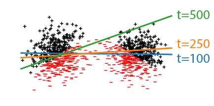
Consider the two-class classification problem in Figure 1 where the two groups are drawn from Gaussians and the optimal classification boundary is given along $x_2 = 0$. Assume that the sampling distribution evolves according to Definition 1 with $\nu(x) = 1.0-x$, $\ell$ equal to the zero one loss, and $b_0=b_1=n^{(0)}_0=n^{(0)}_1=1000$. Initially, ERM has similar and high accuracy on both groups with the boundary $x_2>0$, but over time random fluctuations in accuracy result in slightly fewer samples from the cluster on the right. This leads to disparity amplification since ERM will further improve the loss on the left cluster at the expense of the right cluster. After 500 rounds, there are nearly no samples from the right cluster, and as a result, the right cluster ends up suffering high loss.

3.2 Conditions for disparity amplification

The example above demonstrated that disparity amplification can occur easily even in a situation where the two groups have identical population size and initial risk. In general if we view the expected user counts $\lambda^{(t)}$ as a dynamical system, the long-term fairness properties for any fairness criteria are controlled by two factors - whether $\lambda$ has a fair fixed point (defined as a population fraction where risk minimization maintains the same population fraction over time) and whether this fixed point is stable.

Fixed points of risk minimization are determined by a combination of user retention function $\nu$ and the models $\theta^{(t)}$, and without knowledge of $\nu$ it is hard to ensure that a model has a fair fixed point. Even if a fixed point is fair, such as when the population fraction and risk received by each group is equal, and we start at this fair fixed point, minimizing the empirical loss may deviate from this fair fixed point over time due to finite sample fluctuations or noise in the model estimation procedure.

To show this result, we study the dynamical system $\Phi$, which is defined by dynamics in Definition 1 with $\theta$ derived from minimizing the population, rather than empirical risk.

########## {caption="Definition"}

Let $\Phi$ be the update for the expected population size

$ \lambda^{(t+1)}_k := \Phi(\lambda^{(t)}_k) = \lambda^{(t)}_k \nu(\mathcal{R}_k(\theta(\lambda^{(t)}_k)))+ b_k, $

$ \theta(\lambda^{(t)}k) = \arg\min\theta \mathbb{E}_{\sum_k \alpha_k^{(t)}P_k} [\ell(\theta; Z)]. $

The arrival intensity $\lambda^*$ is called a fixed point if $\lambda^* = \Phi(\lambda^*)$. This fixed point is stable whenever the maximum modulus of the eigenvalues of the Jacobian of $\Phi$ is less than one and unstable whenever it is greater than one ([23], Theorem 2.1).

Proposition 2 gives a precise statement of this phenomenon. We prove the result in Appendix A.1, and further show a generalization to general dynamics $\Phi(\lambda_k) = h(\lambda_k, \mathcal{R}k)$ where $h$ is differentiable and monotone in the second argument. We denote by $\rho{\rm max}(A)$ the maximum modulus of the eigenvalues of $A$.

########## {caption="Proposition 2"}

Let $\lambda^* = \Phi(\lambda^*)$ be a fixed point, and $\theta^* = \arg\min_\theta \mathbb{E}_{\sum_k \alpha_k^* P_k}[\ell(\theta; Z)]$ be the minimizer at $\lambda^*$.

Define $H_{\mathcal{R}}(\alpha^*)$ as the positive definite Hessian of the expected risk at $\theta^*, \lambda^*$ and define $\nabla L$ as the per-group parameter gradients at $\theta^*$,

$ \nabla L = \begin{bmatrix} \nabla_\theta \mathbb{E}{P_1}[\ell(\theta^*; Z)] \ \vdots\ \nabla\theta \mathbb{E}_{P_k}[\ell(\theta^*; Z)]\ \end{bmatrix}. $

The arrival intensity $\lambda^*$ is unstable whenever

$ \begin{split} \rho_{\rm max}\bigg(\mathop{\rm diag}(\nu(\mathcal{R}(\theta(\lambda^*))))

• \mathop{\rm diag}(\lambda^* \nu'(\mathcal{R}(\theta(\lambda^*)) \ \nabla L H_{\mathcal{R}}(\alpha^*)^{-1} \nabla L^\top \left(\frac{I}{\sum_k \lambda^*_k} - \frac{\mathbf{1} \lambda^{\top}}{(\sum_k\lambda^_k)^2}\right) \bigg) > 1. \end{split} $

We see that the major quantities which control risk are the retention rate $\nu$ and its derivative, as well as a $K \times K$ square matrix $\nabla L H_{\mathcal{R}}(\alpha^*)^{-1} \nabla L^\top$ which roughly encodes the changes in one group's risk as a function of another.

We can specialize the stability condition to obtain an intuitive and negative result for the stability of risk minimization (average case). Even if we start at a fair fixed point with $\lambda^*_1 = \cdot s =\lambda^*_k$ and $\mathcal{R}_1 = \cdot s = \mathcal{R}_k$, if decreasing the risk for one group increases the risk for others sufficiently, the fixed point is unstable and the model will eventually converge to a different, possibly unfair, fixed point.

########## {caption="Corollary 3: Counterexample under symmetry"}

Let $\lambda^*_1 = \cdot s = \lambda^*_k$ be a fixed point with $\mathcal{R}_1 = \cdot s = \mathcal{R}_k$, then for any strongly convex loss,

$ \rho_{\rm max}\bigg(\nabla L H_{\mathcal{R}}(\alpha^*)^{-1} \nabla L^\top \bigg) > \frac{1 - \nu(\mathcal{R}_1)}{- \nu'(\mathcal{R}_1)/k}.\tag{3} $

is a sufficient condition for instability.

See Appendix A.2 for proof and generalizations.

The bound Equation 3 has a straightforward interpretation. The left hand side is the stability of the model, where maximal eigenvalue of the matrix $\nabla L H_{\mathcal{R}}(\alpha^*)^{-1} \nabla L^\top$ represents the maximum excess risk that can be incurred due to a small perturbation in the mixture weights $\alpha$. The right hand side represents the underlying stability of the dynamics and measures the sensitivity of $\lambda$ with respect to risk.

Mean and median estimation: Consider a simple mean estimation example where each user belongs to one of two groups, $-1$ or $1$ and incurs loss $(\theta - Z)^2$. $\theta=0$ is clearly a fair fixed point, since it equalizes losses to both groups, with $H_{risk}(\alpha^*) = 1/2$ and $\nabla L = [2, -2]$ making $\rho_{\rm max}\bigg(\nabla L H_{\mathcal{R}}(\alpha^*)^{-1} \nabla L^\top \bigg) = 4$. If we select $\nu(x) = \exp(-x)$, the right hand side becomes $2(1-e^{-1})e $ $\approx 3$ $.4$, and thus any perturbation will eventually result in $\lambda_1 \neq \lambda_2$. In this case the only other fixed points are the unfair solutions of returning the mean of either one of the groups.

The situation is even worse for models which are not strongly convex, such as median estimation. Replacing the squared loss above with the absolute value results in a loss which has a non-unique minimizer at $0$ when $\lambda_1 = \lambda_2$ but immediately becomes $-1$ whenever $\lambda_1 > \lambda_2$. In this case, no conditions on the retention function $\nu$ can induce stability. This fundamental degeneracy motivates us to search for loss minimization schemes with better stability properties than ERM (average case).

4. Distributionally robust optimization (DRO)

Section Summary: The section describes how distributionally robust optimization guards against worst-case performance on unknown subgroups by minimizing an objective that considers all plausible reweightings of the data distribution inside a chi-squared ball. This is achieved by upweighting high-loss examples so that any poorly performing mixture component receives more emphasis during training, thereby bounding the maximum group risk without requiring explicit group labels. The resulting procedure, analyzed through its dual form, produces lower bounds on the smallest group proportion and thereby limits the compounding of representation disparities across successive time steps.

Recall that our goal is to control the worst-case risk Equation 2 over all groups and over all time steps $t$. We will proceed in two steps. First, we show that performing distributionally robust optimization controls the worst-case risk $\mathcal{R}\text{max}(\theta^{(t)})$ for a single time step. Then, we show that this results in a lower bound on group proportions ${ \alpha_k^{(t)} }{k=1}^K$, and thus ensures control over the worst-case risk for all time steps. As a result of the two steps, we show in Section 4.4 that our procedure mitigates disparity amplification over all time steps. For notational clarity, we omit the superscript $t$ in Section 4.1-Section 4.3.

4.1 Bounding the risk over unknown groups

The fundamental difficulty in controlling the worst-case group risk over a single time-step $\mathcal{R}\text{max}(\theta^{(t)})$ comes from not observing the group memberships from which the data was sampled. For many machine learning systems such as speech recognition or machine translation, such situations are common since we either do not ask for sensitive demographic information, or it is unclear a priori which demographics should be protected. To achieve reasonable performance across different groups, we postulate a formulation that protects against all directions around the data generating distribution. We build on the distributionally robust formulation of [24] which will allow us to control the worst-case group risk $\mathcal{R}\text{max}(\theta^{(t)})$.

To formally describe our approach, let $D_{{ \chi^2}}\left(P |!| Q\right)$ be the $\chi^2$-divergence between probability distributions $P$ and $Q$ given by $D_{{ \chi^2}}\left(P |!| Q\right) := \int \left(\frac{dP}{dQ} - 1 \right)^2 dQ$. If $P$ is not absolutely continuous with respect to $Q$, we define $D_{{ \chi^2}}\left(P |!| Q\right) := \infty$.

Let $\mathcal B(P, r)$ be the chi-squared ball around a probability distribution $P$ of radius $r$ so that $\mathcal B(P, r) := { Q \ll P : D_{{ \chi^2}}\left(Q |!| P\right) \le r }$. We consider the worst-case loss over all $r$-perturbations around $P$,

$ \mathcal{R}{\rm dro} (\theta; r) := \sup{Q \in \mathcal B(P, r)} \mathbb{E}_Q[\ell(\theta; Z)].\tag{4} $

Intuitively, the distributionally robust risk $\mathcal{R}{\rm dro}(\theta; r)$ upweights examples $Z$ with high loss $\ell(\theta; Z)$. If there is a group suffering high loss, the corresponding mixture component will be over-represented (relative to the original mixture weights) in the distributionally robust risk $\mathcal{R}{\rm dro}(\theta; r)$. We show in the following proposition that $\mathcal{R}_{\rm dro}(\theta; r)$ bounds the risk of each group $\mathcal{R}_k(\theta)$, and hence the group-wise worst-case risk Equation 1, for an appropriate choice of the robustness radius $r$.

########## {caption="Proposition 4"}

For $P := \sum_{k\in [K]} \alpha_k P_k$, we have $\mathcal{R}k(\theta) \le \mathcal{R}{\rm dro}(\theta; r_k)$ for all $\theta \in \Theta$ where $r_k := \left(1/\alpha_k-1\right)^2$ is the robustness radius.

We prove the result in Appendix A.4. Roughly speaking, the above bound becomes tighter if the variation in the loss $\ell(\theta; Z)$ is substantially higher between groups than within each group. In particular, this would be the case if the loss distribution for each group have distinct support with relatively well-concentrated components within each group.

As a consequence of Proposition 4, if we have a lower bound on the group proportions $\alpha_\text{min} \le \min_{k \in [K]} \alpha_k$, then we can control the worst-case group risk $\mathcal{R}\text{max}(\theta)$ by minimizing the upper bound $\theta \mapsto \mathcal{R}{\rm dro}(\theta; r_{\rm max})$ where $r_{\rm max} := (1/\alpha_\text{min} - 1)^2$.

Similar formulations for robustness around the empirical distribution with radius shrinking as $r / n$ had been considered in ([25, 26, 27]). While there are many possible robustness balls $\mathcal B$ which could provide upper bounds on group risk, we opt to use the chi-squared ball since it is straightforward to optimize ([25, 28, 29]) and we found it empirically outperformed other $f$-divergence balls.

4.2 Interpreting the dual

The dual of the maximization problem Equation 4 provides additional intuition on the behavior of the robust risk.

########## {caption="Proposition 5: ([30])"}

If $\ell(\theta; \cdot)$ is upper semi-continuous for any $\theta$, then for $r_{\rm max} \ge 0$ and any $\theta$, $\mathcal{R}{\rm dro}(\theta; r{\rm max})$ is equal to the following expression

$ \inf_{\eta \in \mathbb{R}} \left{ F(\theta; \eta) := C \left(\mathbb{E}_P\left[\left[{\ell(\theta, Z) - \eta}\right] _+^2\right]\right)^{\frac{1}{2}} + \eta \right}\tag{5} $

where $C = \left(2 (1/\alpha_\text{min} - 1)^2 + 1\right)^{1/2}$.

Denoting by $\eta ^\star$ the optimal dual variable Equation 5, we see from the proposition that all examples suffering less than $\eta ^\star$-levels of loss are completely ignored, and large losses above $\eta ^\star$ are upweighted due to the squared term.

However, unlike standard parameter regularization techniques, which encourage $\theta$ to be close to some point, our objective biases the model to have fewer high loss examples which matches our goal of mitigating representation disparity.

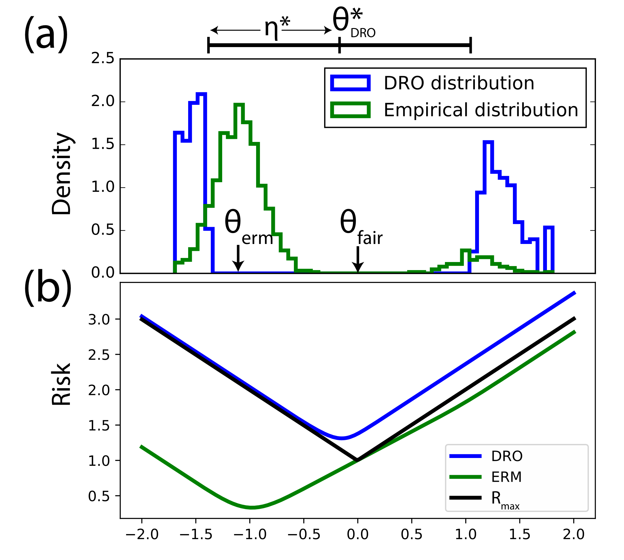
Median Estimation: Recall the median estimation problem over two groups mentioned in Section 3.2 where the loss is $\ell(\theta; Z) = | \theta-Z|1$. Figure 2 shows the behavior of both ERM and DRO on this median estimation task with unbalanced ($\alpha{\min} = 0.1$) groups. The parameter estimate which minimizes $\mathcal{R}\text{max}$ for this problem is $\theta{\text{fair}}=0$ since this is equidistant from both groups. ERM on the other hand focuses entirely on the majority and returns $\theta_{\text{ERM}}\approx -1.0$.

DRO returns $\theta^*_{\text{DRO}}$ which is close to $\theta_{\text{fair}}$. Analyzing the risk, we find that the single-step worst-case group risk $\mathcal{R}\text{max}(\theta)$ in Equation 1 is an upper bound on ERM, and DRO forms a tight upper bound this quantity (Figure 2 b). We can also understand the behavior of DRO through the worst-case distribution $Q$ in Equation 4. Figure 2 a shows the worst-case distribution $Q$ at the minimizer $\theta^*{\text{DRO}}$ which completely removes points within distance $\eta^*$. Additionally, points far from $\theta^*_{\text{DRO}}$ are upweighted, resulting in a large contribution to the loss from the minority group.

We expect the bound to be tight when all individuals within a group receive the same loss. In this case, thresholding by $\eta^*$ corresponds to selecting the single highest risk group which is equivalent to directly minimizing $\mathcal{R}_\text{max}(\theta)$ Equation 1.

On the other hand, the worst case for our approach is if $\alpha_{\min}$ is small, and a group with low expected loss has a high loss tail with population size $\alpha_{\min}$. In this case DRO is a loose upper bound and optimizes the losses of the group with already low expected loss.

This is closely related to recent observations that the DRO bound can be loose for classification losses such as the zero-one loss due to the worst-case distribution consisting purely of misclassified examples [31]. Even in this case, the estimated loss is still a valid upper bound on the worst case group risk, and as Figure 2 shows, there are examples where the DRO estimate is nearly tight.

4.3 Optimization

We now show how to minimize $\theta \mapsto \mathcal{R}{\rm dro}(\theta; r{\rm max})$ efficiently for a large class of problems. For models such as deep neural networks that rely on stochastic gradient descent, the dual objective $F(\theta; \eta)$ in Equation 5 can be used directly since it only involves an expectation over the data generating distribution $P$.

Formally, the following procedure optimizes Equation 4: for a given value of $\eta$, compute the approximate minimizer $\widehat{\theta}_\eta$

$ \mathop{\rm minimize}{\theta \in \Theta} \mathbb{E}{P}\left[{\ell(\theta; Z)-\eta}\right] _+^2.\tag{6} $

From Proposition 4 and Proposition 5, we have

$ \mathcal{R}\text{max}(\widehat{\theta}\eta) \le \mathcal{R}{\rm dro}(\widehat{\theta}\eta; r_{\rm max}) \le F(\widehat{\theta}_{\eta}, \eta) $

which implies that we can treat $\eta$ as a hyperparameter. For convex losses $\theta \mapsto \ell(\theta; Z)$, the function $\eta \mapsto F(\widehat{\theta}_{\eta}, \eta)$ is convex, and thus we can perform a binary search over $\eta$ to find the global optimum efficiently.

Alternatively, for models where we can compute $\theta^*(Q) \in \mathop{\rm argmin}_{\theta \in \Theta} \mathbb{E}Q[\ell(\theta; Z)]$ efficiently, we can use existing primal solvers that compute the worst-case probability distribution $Q^*(\theta) \in \mathop{\rm argmax}{Q \in \mathcal B(P, r)} \mathbb{E}_Q[\ell(\theta; Z)]$ for a given $\theta$ based on projected gradient ascent on $Q$ ([28]). By alternating between optimization on $\theta$ and $Q$, we can efficiently find the saddle point $(\theta^*, Q^*)$ that satisfies $\theta^* = \theta^*(Q^*)$ and $Q^* = Q^*(\theta^*)$.

4.4 Stability of minority loss minimization

We have thus far demonstrated that for a single time step, the worst-case risk over all groups $\mathcal{R}\text{max}(\theta) = \max_k \mathcal{R}k(\theta)$ can be controlled by the distributionally robust risk $\mathcal{R}{\rm dro}(\theta; r{\rm max})$ where $r_{\rm max} := (1/\alpha_\text{min} - 1)^2$ and $\alpha_\text{min}$ is the minority group proportion. Now, we study how the individual group risk $\mathcal{R}k(\theta)$ affects user retention and hence future risk. By virtue of providing an upper bound to $\mathcal{R}\text{max}(\theta)$, optimizing $\mathcal{R}{\rm dro}(\theta; r{\rm max})$ at each time step can thus control the future group risk $\mathcal{R}_\text{max}(\theta)$.

We show that if the initial group proportions satisfy $\alpha_k^{(0)} \ge \alpha_\text{min}$ and the worst-case risk $\mathcal{R}\text{max}(\theta^{(t)})$ is sufficiently small at each time $t$, then we can ensure $\alpha_k^{(t+1)} > \alpha\text{min}$. Thus, to control $\mathcal{R}\text{max}^{T}$, the worst-case group risk over all time steps, it suffices to control $\mathcal{R}{\rm dro}(\theta^{(t)}; r_{\rm max})$ using the procedure in Section 4.3.

########## {caption="Proposition 6"}

Assume the retention model in Definition 1. Let $\alpha_k^{(t)} > \alpha_\text{min}$, $\frac{b_k}{\sum_k b_k} > \alpha_\text{min}$, $\lambda^{(t)}:= \sum_k \lambda_k^{(t)} \leq \frac{\sum_k b_k}{1-\nu_{\max}}$, and $\nu(\mathcal{R}k(\theta^{(t)})) < \nu{\max}$. Then, whenever we have

$ \mathcal{R}k(\theta^{(t)}) \leq \nu^{-1}\left(1 - \frac{(1-\nu{max})b_k}{\alpha_\text{min} \sum_k b_k}\right), $

$ \alpha_k^{(t+1)} = \frac{\lambda^{(t)}\alpha_k^{(t)} \nu(\mathcal{R}_k(\theta^{(t)}))+b_k}{\sum_l \lambda^{(t)}\alpha_l^{(t)} \nu(\mathcal{R}l(\theta^{(t)}))+b_l} > \alpha\text{min}. $

We conclude that as long as we can guarantee

$ \mathcal{R}{\rm dro}(\theta^{(t)}; r{\rm max}) \le \nu^{-1}\left(1 - \frac{(1-\nu_{max})b_k}{\alpha_\text{min} \sum_k b_k}\right),\tag{7} $

we can control $\mathcal{R}\text{max}^T(\theta^{(0)}, \ldots, \theta^{(T)})$, the unknown worst-case group risk over all time steps by optimizing $\mathcal{R}{\rm dro}(\theta^{(t)}; r_{\rm max})$ at each step $t$. While the condition Equation 7 is hard to verify in practice, we observe empirically in Section 5 that optimizing the distributionally robust risk $\mathcal{R}{\rm dro}(\theta^{(t)}; r{\rm max})$ at time step $t$ indeed significantly reduces disparity amplification in comparison to using ERM.

Proposition 6 gives stronger fairness guarantees than the stability conditions for ERM in Proposition 2. In ERM the best one can do is to add strong convexity to the model to stabilize to a possibly unfair fixed point. In contrast, Proposition 6 gives conditions for controlling $\mathcal{R}_\text{max}$ over time without assuming that there exists a fair fixed point.

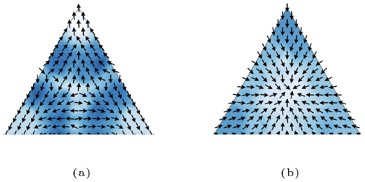
Stability of median estimation: Returning to our running example of geometric median estimation, we can show that under the same dynamics, ERM is highly unstable while DRO is stable. Consider a three Gaussian mixture on the corners of the simplex, with $L_2$ loss, retention function $\nu(r) = \exp(-r)$, and $b_1=b_2=50$, $n^{(t)}=1000$. By construction, $(1/3, 1/3, 1/3)$ is the fair parameter estimate.

Figure 3 shows that ERM is highly unstable, with the only stable fixed points being the corners, where a single group dominates all others. The fair parameter estimate is an unstable fixed point for ERM, and any perturbation eventually results in a completely unfair parameter estimate. On the other hand, DRO has the reverse behavior, with the fair parameter estimate being the unique stable fixed point.

5. Experiments

Section Summary: In experiments, the authors test distributionally robust optimization (DRO) against standard empirical risk minimization on both a simulated classification task and a real text autocomplete system evaluated by humans. In the simulated setting with two imbalanced groups, DRO stabilizes accuracy for the shrinking minority group over repeated rounds of model updates, whereas standard training leads to rapid drops in performance. On the autocomplete task with tweets from different demographic groups, human evaluations via Mechanical Turk show that DRO improves minority-group satisfaction and retention rates while causing only minor trade-offs for the majority group.

We demonstrate the effectiveness of DRO on our motivating example (Figure 1) and human evaluation of a text autocomplete system on Amazon Mechanical Turk. In both cases, DRO controls the worst-case risk $\mathcal{R}_\text{max}^T$ over time steps and improves minority retention.

5.1 Simulated task

Recall the motivating example in Figure 1 which shows that logistic regression applied to a two-class classification problem is unstable and becomes pathologically unfair.

The data is constructed by drawing from a mixture of two Gaussians (groups) centered at $(-1.5, 0)$ and $(0, 1.5)$. The two groups are labeled according to the linear decision boundaries $(-3/2, \sqrt{3^2-1}/3)$ and $(3/2, \sqrt{3^2-1}/3)$ respectively such that classifying with $x_2>0$ is accurate, but the optimal linear classifier on one group achieves 50% accuracy on the other.

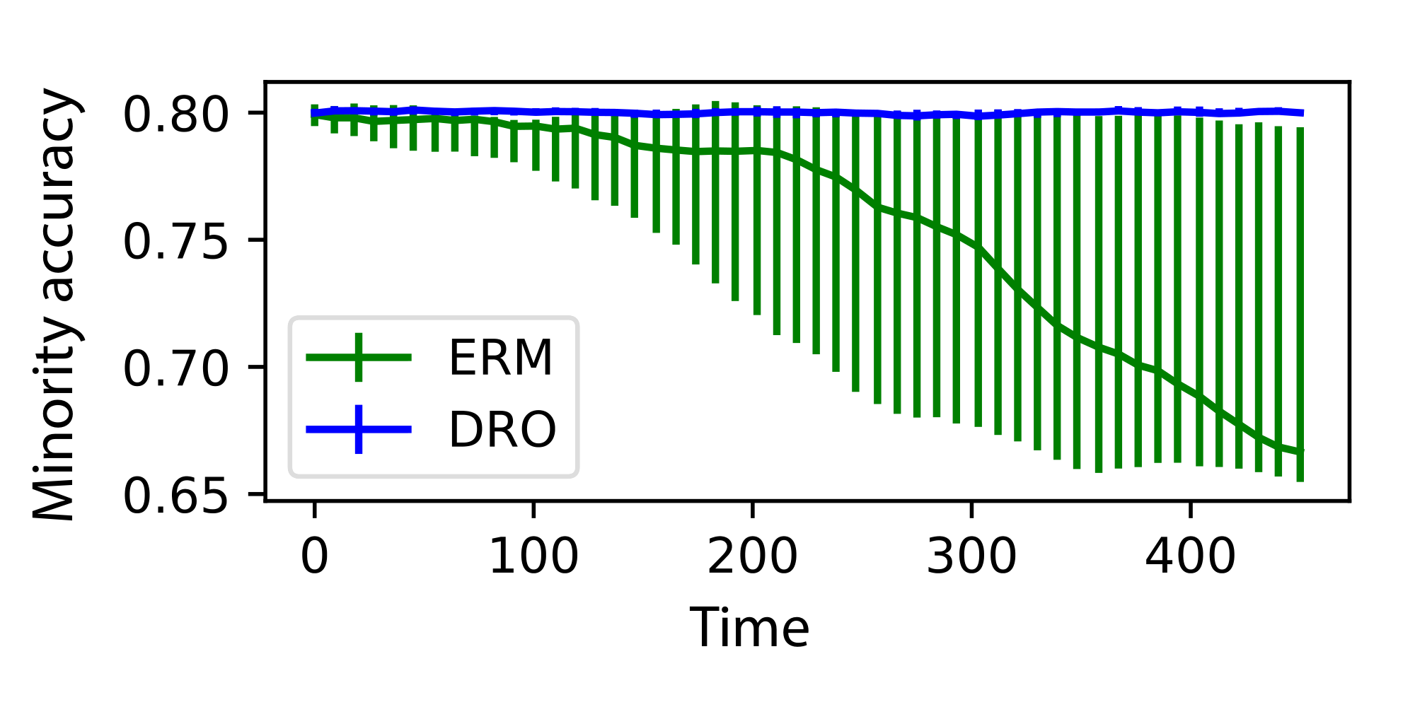
At each round we fit a logistic regression classifier using ERM or DRO and gradient descent, constraining the norm of the weight vector to 1. Our dynamics follow Definition 1 with $\nu(x) = 1-x$, $\mathcal{R}$ as the zero-one loss, and $b_k= 1000$. The DRO model is trained using the dual objective with logistic loss, and $\eta=0.95$, which was the optimal dual solution to $\alpha_{\min} = 0.2$. The results do not qualitatively change for choices of $\alpha_{\min} < 0.5$, and we show that we obtain control even for group sizes substantially smaller than 0.2 (Figure 6).

Figure 5 shows that ERM is unstable and the minority group rapidly loses accuracy beyond $300$ rounds on most runs. In contrast, DRO is stable, and maintains an accuracy of $0.8$.

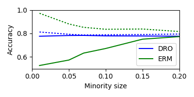
This stability is due to the fact that the regularized loss for DRO prevents small losses in the minority fraction from amplifying, as we discuss in Proposition 6. Even when the minority fraction falls as low as $1%$, the DRO loss ensures that the accuracy of this minority fraction remains at $75%$ accuracy (Figure 6).

5.2 Autocomplete task

We now present a real-world, human evaluation of user retention and satisfaction on a text autocomplete task. The task consists of the prediction of next words in a corpus of tweets built from two estimated demographic groups, African Americans and White Americans ([3]). There are several distinguishing linguistic patterns between tweets from these groups, whose language dialects we henceforth refer to as African-American English (AAE) and Standard-American English (SAE), respectively, following the nomenclature in [3]. Our overall experimental design is to measure the retention rate $\nu$ and risk $\mathcal{R}$ for various choices of demographic proportions $(\alpha_{\text{AAE}}, \alpha_{\text{SAE}})$ and simulate the implied dynamics, since running a fully online experiment would be prohibitively expensive.

For both ERM and DRO, we train a set of five maximum likelihood bigram language models on a corpus with 366, 361 tweets total and a $f \in {0.1, 0.4, 0.5, 0.6, 0.9}$ fraction of the tweets labeled as AAE. This results in 10 possible autocomplete systems a given Mechanical Turk user can be assigned to during a task.

To evaluate the retention and loss for AAE and SAE separately, a turk user is assigned 10 tweets from either the held out AAE tweets or SAE tweets, which they must replicate using a web-based keyboard augmented by the autocomplete system. This assignment of a turk user to a demographic group simulates the situation where a user from a particular demographic group attempts to use the autocomplete system to write a tweet. Details of the autocomplete task are included in the supplement.

After completing the task, users were asked to fill out a survey which included a rank from 1 to 5 on their satisfaction with the task, and a yes/no question asking whether they would continue to use such a system. We assign 50 users to each of the two held out set types and each of the 10 autocomplete models, resulting in 1, 000 users' feedback across autocomplete models and assigned demographics.

The response to whether a user would continue to use the autocomplete system provides samples $\nu(\mathcal{R}_K(\alpha))$ with $n=366361$ and each of possible demographic proportions $\alpha$. The user satisfaction survey provides a surrogate for $\mathcal{R}_K(\alpha)$ at these same points. We interpolate $\nu$ and $\mathcal{R}_K$ to $\alpha \in [0, 1]$ via isotone regression which then allows us to simulate the user dynamics and satisfaction over time using Definition 1. We estimate variability in these estimates via bootstrap replicates on the survey responses.

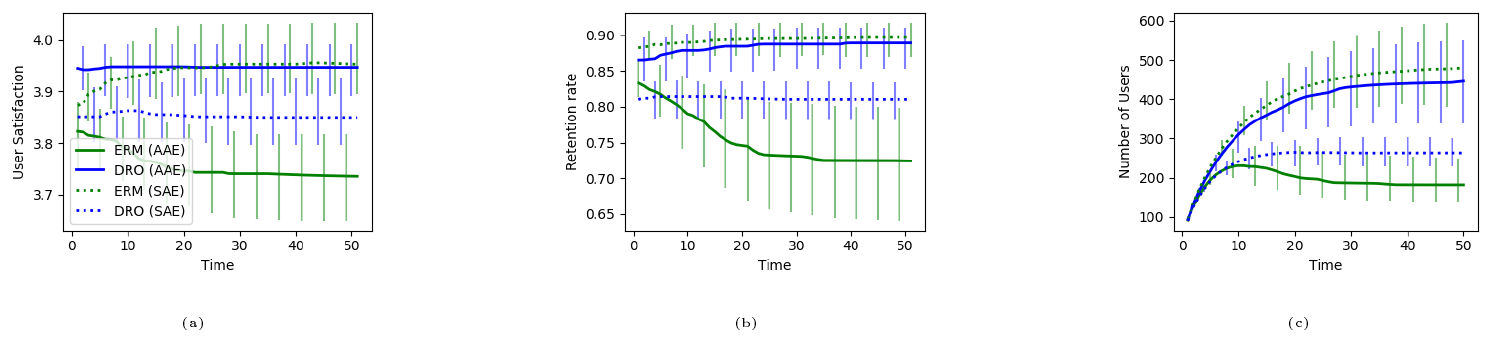
Our results in Figure 4 show an improvement in both minority satisfaction and retention rate due to DRO: we improve the median user satisfaction from 3.7 to 4.0 and retention from 0.7 to 0.85, while only slightly decreasing the SAE satisfaction and retention. Implied user counts follow the same trend with larger differences between groups due to compounding.

Counterintuitively, the minority group has higher satisfaction and retention under DRO. Analysis of long-form comments from Turkers suggest this is likely due to users valuing the model's ability to complete slang more highly than completion of common words and indicates a slight mismatch between our training loss and human satisfaction with an autocomplete system.

6. Discussion

Section Summary: In this paper the authors frame loss minimization in machine learning as a problem of distributive justice, arguing that standard empirical risk minimization tends to amplify disparities for minority groups while distributionally robust optimization can place an upper bound on those groups’ risks. Their position echoes Rawlsian critiques of utilitarianism, yet they note that it inherits well-known objections to that philosophical stance and leave the search for a better ethical grounding to future work. They close by identifying two open issues: the observational nature of their method makes it unsuitable for high-stakes decisions involving known demographic groups, and distributional robustness clashes with classical outlier rejection, leaving unclear how to achieve both fairness to latent subgroups and resistance to noise.

In this work we argued for a view of loss minimization as a distributive justice problem and showed that ERM often results in disparity amplification and unfairness. We demonstrate that DRO provides a upper bound on the risk incurred by minority groups and performs well in practice. Our proposed algorithm is straightforward to implement, and induces distributional robustness, which can be viewed as a benefit in and of itself.

Our arguments against ERM and in favor of minority risk minimization mirror Rawls' arguments against utilitarianism, and thus inherit the critiques of Rawlsian distributive justice. Examples of such critiques are the focus on an abstract worst-off group rather than demographic groups or individuals [32], extreme risk-aversion [33], and utilitarianism with diminishing returns as an alternative [34]. In this work, we do not address the debate on the correctness of Rawlsian justice ([10]), and leave finding a suitable philosophical framework for loss minimization to future work.

There are two large open questions from our work. First, as fairness is fundamentally a causal question, observational approaches such as DRO can only hope to control limited aspects of fairness. The generality with which our algorithm can be applied also limits its ability to enforce fairness as a constraint, and thus our approach here is unsuitable for high-stakes fairness applications such as classifiers for loans, criminality, or admissions. In such problems the implied minorities from DRO may differ from well-specified demographic groups who are known to suffer from historical and societal biases. This gap arises due to looseness in the DRO bound [31], and could be mitigated using smoothness assumptions [16].

Second, distributional robustness proposed here runs counter to classical robust estimation for rejecting outlier samples, as high loss groups created by an adversary can easily resemble a minority group. Adversarial or high-noise settings loosen the DRO upper bound substantially, and it is an open question whether it is possible to design algorithms which are both fair to unknown latent groups and robust.

Reproducibility: Code to generate results available on the CodaLab platform at https://bit.ly/2sFkDpE.

Acknowledgements: This work was funded by an Open Philanthropy Project Award.

Appendix

Section Summary: The appendix supplies formal proofs establishing when fixed points of an iterative update rule for group population sizes remain stable under a dynamical system. It derives a necessary and sufficient condition on the spectral radius of the Jacobian of the map, obtained by chaining derivatives of the risk, model parameters, and population fractions, and then specializes and generalizes the same argument to a corollary and to broader families of update functions. All steps rely on standard matrix calculus, strong convexity of the loss, and first-order optimality conditions at the equilibrium.

A.1 Proof of Proposition 2

We prove the following more general result.

########## {caption="Proposition"}

Let $\lambda^* = \Phi(\lambda^*)$ be a fixed point, and $\theta^* = \arg\min_\theta \mathbb{E}_{\sum_k \alpha_k^* P_k}[\ell(\theta; Z)]$ be the population minimizer.

Define $H_{\mathcal{R}}(\alpha^*)$ as the positive definite Hessian of the expected risk with $\alpha_k^* \propto \lambda^*_k$.

Further, let $\nabla L$ define the per-group parameter gradients at $\theta^*$,

$ \nabla L = \begin{bmatrix} \nabla_\theta \mathbb{E}{P_1}[\ell(\hat{\theta}; Z)] \ \vdots\ \nabla\theta \mathbb{E}_{P_k}[\ell(\hat{\theta}; Z)]\ \end{bmatrix}. $

$\lambda^*$ is stable whenever the absolute value of the maximum eigenvalue $\rho_{\max}$ obeys

$ \rho_{\max}\bigg(\mathop{\rm diag}(\nu(\mathcal{R}(\theta(\lambda^*))))

• \mathop{\rm diag}(\lambda^* \nu'(\mathcal{R}(\theta(\lambda^*)) \nabla L H_{\mathcal{R}}(\alpha^*)^{-1} \nabla L^\top \left(\frac{I}{\sum_k \lambda^*_k} - \frac{\mathbf{1} \lambda^{\top}}{(\sum_k\lambda^_k)^2}\right) \bigg) < 1. $

Proof: A necessary and sufficient condition for stability of a discrete time dynamical system is that the Jacobian of the forward map $\Phi$ has eigenvalues with absolute value strictly less than 1.

Computing the Jacobian we have:

$ \mathbf{J}_{\Phi}(\lambda^*) = \mathop{\rm diag}(\nu(\mathcal{R}_k(\lambda^*)))

• \mathop{\rm diag}(\lambda^* \nu'(\mathcal{R}(\theta(\lambda^*))))\mathbf{J}_{\mathcal{R}\circ \theta \circ \alpha^*}(\lambda^*). $

Now we must compute the Jacobian of the risk with respect to the population fraction. To do this, we apply the chain rule and separately analyze three Jacobians: $\mathcal{R}$ with respect to $\theta$, $\theta$ with respect to $\alpha^*$, and $\alpha^*$ with respect to $\lambda^*$

By strong convexity of $\ell$,

$ \mathbf{J}{\theta}(\alpha^*) = - H{\mathcal{R}}(\alpha^*)^{-1} \nabla L^\top. $

Where $H_{\mathcal{R}}(\alpha^*)^{-1}$ is the Hessian of the population risk and $\nabla L$ is

$ \nabla L = \begin{bmatrix} \nabla_\theta \mathbb{E}{P_1}[\ell(\hat{\theta}; Z)] \ \vdots\ \nabla\theta \mathbb{E}_{P_k}[\ell(\hat{\theta}; Z)]\ \end{bmatrix}. $

The Jacobian of the risks with respect to change in $\theta$ is

$ \mathbf{J}_{\mathcal{R}}(\theta) = \nabla L. $

The Jacobian of the population fraction with respect to $n$ is

$ \mathbf{J}_{\alpha^*}(\lambda^*) = \left(\frac{I}{\sum_k \lambda^*_k} - \frac{\mathbf{1}\lambda^{\top}}{(\sum_k \lambda^_k)^2}\right) $

By the chain rule, we obtain the overall claim

$ \mathbf{J}_{\Phi}(\lambda^*) = \mathop{\rm diag}(\nu(\mathcal{R}_k(\lambda^*)))

• \mathop{\rm diag}(\lambda^* \nu'(\mathcal{R}(\theta)))\nabla L H_{\mathcal{R}}(\alpha^*)^{-1} \nabla L^\top \left(\frac{I}{\sum_k \lambda^*_k} - \frac{\mathbf{1}\lambda^{\top}}{(\sum_k \lambda^_k)^2}\right) $

A.2 Proof of Corollary 3

Recall that the instability criteria is

$ \rho_{\max}\bigg(\mathop{\rm diag}(\nu(\mathcal{R}(\theta(\lambda^*))))

• \mathop{\rm diag}(\lambda^* \nu'(\mathcal{R}(\theta(\lambda^*)) \nabla L H_{\mathcal{R}}(\alpha^*)^{-1} \nabla L^\top \left(\frac{I}{\sum_k \lambda^*_k} - \frac{\mathbf{1} \lambda^{\top}}{(\sum_k\lambda^_k)^2}\right) \bigg) > 1. $

Setting $\nu(\mathcal{R}(\theta(\lambda^*))) = \nu(\mathcal{R}_1)$ and $\lambda^*_k = \lambda^*_1$ we have,

$ \rho_{\max}\bigg(- \nu'(\mathcal{R}1) \nabla L H{\mathcal{R}}(\alpha^*)^{-1} \nabla L^\top \left(I/k - \mathbf{1} \mathbf{1}^{\top}/k^2\right) \bigg) > 1 - \nu(\mathcal{R}_1). $

By first order optimality conditions, and the fact that $\lambda^*_1 \cdot s = \lambda^*_k$, $\nabla L^\top \mathbf{1}=0$.

Thus, collecting terms and noting $\nu'(x) < 0$ by monotonicity of $\nu$, we have

$ \rho_{\max}\bigg(\nabla L H_{\mathcal{R}}(\alpha^*)^{-1} \nabla L^\top \bigg) > \frac{1 - \nu(\mathcal{R}_1)}{- \nu'(\mathcal{R}_1)/k}. $

A.3 Generalization of Proposition 2 and Corollary 3

Consider the more general dynamics defined by $h: (\lambda, \mathcal{R}) \to \mathbb{R}^+$ which defines the evolution of the expected number of users.

########## {caption="Definition"}

Let $\Phi$ be the update for the expected population size

$ \lambda^{(t+1)}_k := \Phi(\lambda^{(t)}_k) = h(\lambda^{(t)}_k, \nu(\mathcal{R}_k(\theta(\lambda^{(t)})))), $

$ \theta(\lambda^{(t)}k) = \arg\min\theta \mathbb{E}_{\sum_k \alpha_k^{(t)}P_k} [\ell(\theta; Z)]. $

Then as long as $h$ is differentiable in both arguments, we obtain an essentially identical result to before.

########## {caption="Proposition"}

Let $\lambda^* = \Phi(\lambda^*)$ be a fixed point, and $\theta^* = \arg\min_\theta \mathbb{E}_{\sum_k \alpha_k^* P_k}[\ell(\theta; Z)]$ be the population minimizer.

Define $H_{\mathcal{R}}(\alpha^*)$ as the positive definite Hessian of the expected risk with $\alpha_k^* \propto \lambda^*_k$.

Further, let $\nabla L$ define the per-group parameter gradients at $\theta^*$,

$ \nabla L = \begin{bmatrix} \nabla_\theta \mathbb{E}{P_1}[\ell(\hat{\theta}; Z)] \ \vdots\ \nabla\theta \mathbb{E}_{P_k}[\ell(\hat{\theta}; Z)]\ \end{bmatrix}. $

$\lambda^*$ is stable whenever

$ \rho_{\max}\left(\mathop{\rm diag}\left(\frac{\partial}{\partial \lambda} h(\lambda^*, \mathcal{R}(\theta(\lambda^*)))\right)

• \mathop{\rm diag}\left(\frac{\partial}{\partial \mathcal{R}} h(\lambda^*, \mathcal{R}(\theta(\lambda^*)))\right) \nabla L H_{\mathcal{R}}(\alpha^*)^{-1} \nabla L^\top \left(\frac{I}{\sum_k \lambda^*_k} - \frac{\mathbf{1} \lambda^{\top}}{(\sum_k\lambda^_k)^2}\right) \right) < 1. $

Proof: A necessary and sufficient condition for stability of a discrete time dynamical system is that the Jacobian of the forward map $\Phi$ has eigenvalues with absolute value strictly less than 1.

Computing the Jacobian via total derivatives we have

$ \mathbf{J}_{\Phi}(\lambda^*) = \mathop{\rm diag}\left(\frac{\partial}{\partial \lambda} h(\lambda^*, \mathcal{R}(\theta(\lambda^*)))\right)

• \mathop{\rm diag}\left(\frac{\partial}{\partial \mathcal{R}} h(\lambda^*, \mathcal{R}(\theta(\lambda^*)))\right) \mathbf{J}_{\mathcal{R}\circ \theta \circ p}(\lambda^*). $

The Jacobian term remains identical to before, which completes the proof.

The Corollary follows from this derivation:

########## {caption="Corollary 3: Counterexample under symmetry"}

Let $\lambda^*_1 = \cdot s \lambda^*_k$ be a fixed point with $\mathcal{R}_1 = \cdot s \mathcal{R}k$, and define $\frac{\partial h}{\partial \lambda} \big|{\lambda=\lambda^*} = \frac{\partial}{\partial \lambda} h(\lambda^*_1, \mathcal{R}1)$ and $\frac{\partial h}{\partial \mathcal{R}} \big|{\lambda=\lambda^*} = \frac{\partial}{\partial \mathcal{R}} h(\lambda^*_1, \mathcal{R}_1)$. For any strongly convex loss,

$ \rho_{\max}\bigg(\nabla L H_{\mathcal{R}}(\alpha^*)^{-1} \nabla L^\top \bigg) > \frac{1 - \frac{\partial h}{\partial \lambda} \big|{\lambda=\lambda^*}}{- \frac{\partial h}{\partial \mathcal{R}} \big|{\lambda=\lambda^*}}k\lambda^*_1. $

Proof: Recall that the instability criteria is

$ \rho_{\max}\left(\mathop{\rm diag}\left(\frac{\partial}{\partial \lambda} h(\lambda^*, \mathcal{R}(\theta(\lambda^*)))\right)

• \mathop{\rm diag}\left(\frac{\partial}{\partial \mathcal{R}} h(\lambda^*, \mathcal{R}(\theta(\lambda^*)))\right) \nabla L H_{\mathcal{R}}(\alpha^*)^{-1} \nabla L^\top \left(\frac{I}{\sum_k \lambda^*_k} - \frac{\mathbf{1} \lambda^{\top}}{(\sum_k\lambda^_k)^2}\right) \right) < 1. $

Let $\frac{\partial h}{\partial \lambda} \big|_{\lambda=\lambda^*} = \frac{\partial}{\partial \lambda} h(\lambda^*_1, \mathcal{R}1(\theta(\lambda^*)))$ and $\frac{\partial h}{\partial \mathcal{R}} \big|{\lambda=\lambda^*} = \frac{\partial}{\partial \mathcal{R}} h(\lambda^*_1, \mathcal{R}_1(\theta(\lambda^*)))$. Then following the same derivation as earlier and using the monotonicity of $h$ in the second argument gives

$ \rho_{\max}\bigg(\nabla L H_{\mathcal{R}}(\alpha^*)^{-1} \nabla L^\top \bigg) > \frac{1 - \frac{\partial h}{\partial \lambda} \big|{\lambda=\lambda^*}}{- \frac{\partial h}{\partial \mathcal{R}} \big|{\lambda=\lambda^*}}k\lambda^*_1. $

This is essentially in the same spirit as our earlier corollary, but requires further assumptions on $h$ in order to interpret. Generally we expect $\frac{\partial h}{\partial R}$ to be on the order of $\lambda$ as long as risk affects users independently, and $\frac{\partial h}{\partial \lambda}$ is upper bounded by the maximum implied retention rate.

A.4 Proof of Proposition 4

Since $P_k$ is a mixture component of $P$ ($P = \alpha_k P_k + \cdot s$),

$ \begin{aligned} D_{{ \chi^2}}\left(P_k |!| {P^{(t)}}\right) &= \int_x \left(\frac{P_k^{(t)}(x)}{P^{(t)}(x)}-1 \right)^2 P^{(t)}(x) dx \ &\leq \int_x \left(\frac{1}{ \alpha_k^{(t)}}-1 \right)^2 P^{(t)}(x) dx \ &= r_k. \end{aligned} $

We just showed that $P_k \in \mathcal B(P, r_k)$. Since the sup is over all $Q \in \mathcal B(P, r_k)$, the upper bound follows.

A.5 Proof of Proposition 6

By assumption,

$ \begin{aligned} \alpha_k^{(t+1)} & \geq \frac{\lambda^{(t)}\alpha_\text{min} \nu(\mathcal{R}_k(\theta^{(t)}))+b_k}{\sum_k \lambda^{(t)}\alpha_k^{(t)} \nu(\mathcal{R}_k(\theta^{(t)}))+b_k}. \end{aligned} $

We will show

$ \frac{\lambda^{(t)}\alpha_\text{min} \nu(\mathcal{R}_k(\theta^{(t)}))+b_k}{\sum_k \lambda^{(t)}\alpha_k^{(t)} \nu(\mathcal{R}k(\theta^{(t)}))+b_k} > \alpha\text{min}, $

which is equivalent to

$ \nu(\mathcal{R}_k(\theta^{(t)})) \geq \sum_k \alpha_k^{(t)} \nu(\mathcal{R}k(\theta^{(t)}))+ \frac{ \sum_k b_k - b_k/\alpha\text{min}}{\lambda^{(t)}}. $

By the assumption that $\nu(\mathcal{R}k(\theta^{(t)})) < \nu{\max}$,

$ \sum_k \alpha_k^{(t)} \nu(\mathcal{R}k(\theta^{(t)}))+ \frac{ \sum_k b_k - b_k/\alpha\text{min}}{\lambda^{(t)}} \leq \nu_{\max} + \frac{\sum_k b_k}{\lambda^{(t)}} \left(1- \frac{b_k}{\alpha_\text{min} \sum_k b_k} \right). $

Using $\frac{b_k}{\sum_k b_k} \geq \alpha_\text{min}$ and $\lambda^{(t)} \leq \frac{\sum b_k}{1-\nu_{\max}}$ the above simplifies to

$ \sum_k \alpha_k^{(t)} \nu(\mathcal{R}k(\theta^{(t)}))+ \frac{ \sum_k b_k - b_k/\alpha\text{min}}{\lambda^{(t)}} \leq \nu_{\max} + (1-\nu_{\max})\left(1-\frac{b_k}{\alpha_\text{min} \sum_k b_k}\right). $

Thus, a sufficient condition for our proposition is

$ \mathcal{R}k(\theta^{(t)}) \leq \nu^{-1}\left(1 - \frac{(1-\nu{max})b_k}{\alpha_\text{min} \sum_k b_k}\right). $

. ## Amazon Mecahnical Turk task description

The Amazon Mechanical Turk experiment modeling user retention in an autocomplete system is detailed below. The experiment design consists of a total of 1000 HITs ("Human Intelligence Tasks" on Mechanical Turk) consisting of 2 user replicates $\times$ 5 values of $\alpha$ $\times$ 2 models (DRO/ERM) $\times$ 25 sets of 10 tweets from the test set $\times$ two test sets (AAE/SAE).

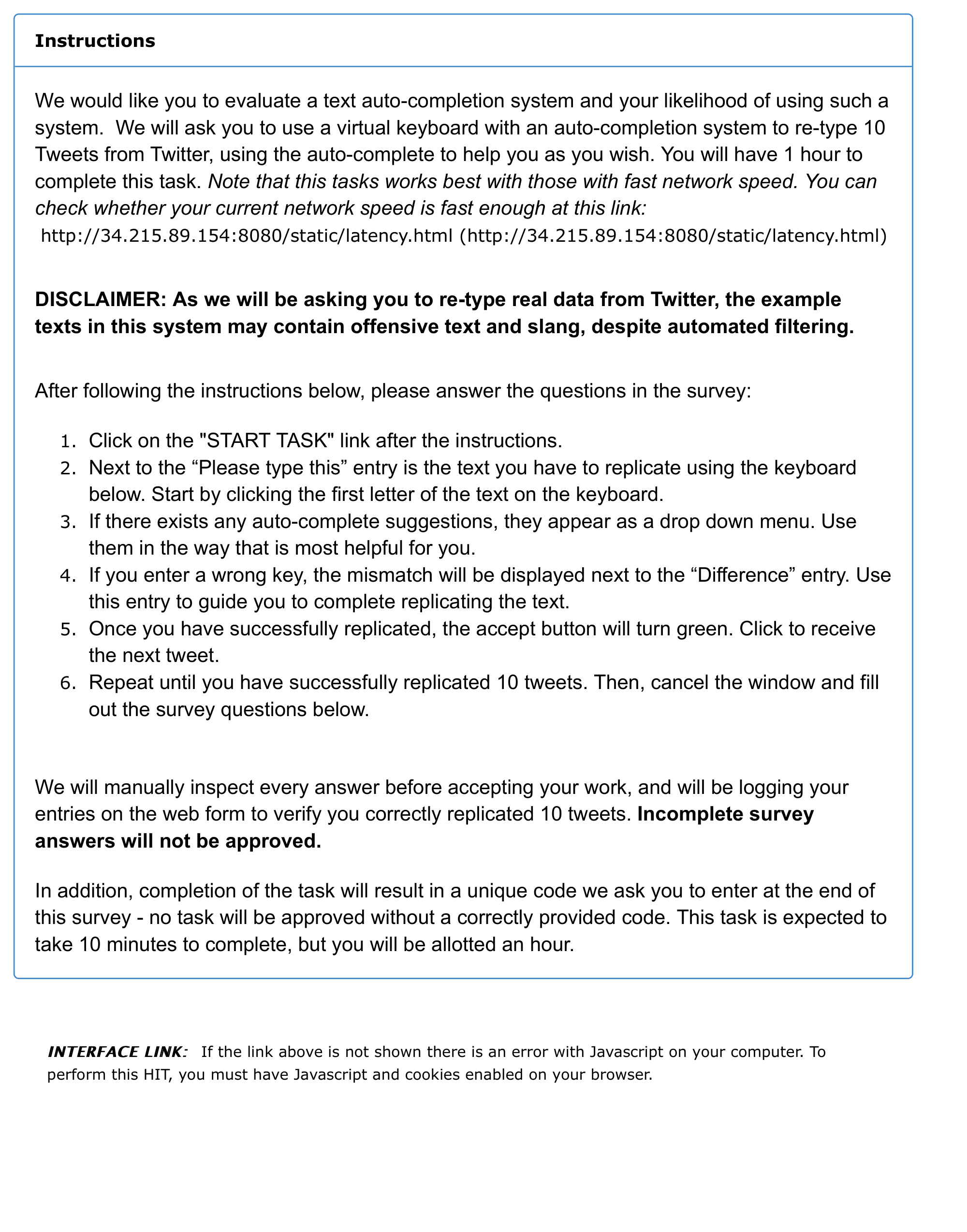
For each HIT the task, users are provided the description given in Figure 7 . Users are then taken to a separate autocomplete website, where they are asked to replicate 10 tweets using a software keyboard shown in Figure 8. In this interface, users must use the mouse and the software keyboard to type the target sentence, while also being given an autocomplete system for next word prediction based on the two models. The autocomplete system appears through a dropdown as users begin typing. After completion to the task, users are prompted to fill out a survey in Figure 9, Figure 10. The first four questions are quality control questions designed to identify Turkers who were low effort (empty entries in Q1/Q3) or inconsistent (Q2 inconsistent with Q4). Moreover, low-quality HITS could easily be identified due to a user's refusal to select either yes or no to Q5. We used this as our metric for filtering which users would be considered in the analysis. Q6 is our overall satisfaction metric shown in the main paper.

References

Section Summary: The references section compiles 34 academic papers, technical reports, and books drawn primarily from machine learning conferences and journals. They cover speech and image recognition systems, documented performance gaps tied to dialect, gender, age, and race, and a cluster of work on algorithmic fairness that incorporates ideas from political philosophy such as Rawls’s theory of justice. A smaller set addresses robust and distributionally robust optimization methods.

[1] Amodei, D. et al. Deep speech 2 end to end speech recognition in English and mandarin. In International Conference on Machine Learning (ICML), pp. 173–182, 2016.

[2] Grother, P. J., Quinn, G. W., and Phillips, P. J. Report on the evaluation of 2d still-image face recognition algorithms. Technical report, NIST, 2011.

[3] Blodgett, S. L., Green, L., and O'Connor, B. Demographic dialectal variation in social media: A case study of African-American English. In Empirical Methods in Natural Language Processing (EMNLP), pp. 1119–1130, 2016.

[4] Jurgens, D., Tsvetkov, Y., and Jurafsky, D. Incorporating dialectal variability for socially equitable language identification. In Association for Computational Linguistics (ACL), pp. 51–57, 2017.

[5] Hovy, D. and Søgaard, A. Tagging performance correlates with age. In Association for Computational Linguistics (ACL), pp. 483–488, 2015.

[6] Sapiezynski, P., Kassarnig, V., Wilson, C., Lehmann, S., and Mislove, A. Academic performance prediction in a gender-imbalanced environment. In FATREC, volume 1, pp. 48–51, 2017.

[7] Tatman, R. Gender and dialect bias in youtube’s automatic captions. In Workshop on Ethics in Natural Langauge Processing, volume 1, pp. 53–59, 2017.

[8] Fuster, A., Goldsmith-Pinkham, P., Ramadorai, T., and Walther, A. Predictably unequal? the effects of machine learning on credit markets. Technical report, CEPR Discussion Papers, 2017.

[9] Barocas, S. and Selbst, A. D. Big data's disparate impact. 104 California Law Review, 3:671–732, 2016.

[10] Rawls, J. Justice as fairness: a restatement. Harvard University Press, 2001.

[11] Chouldechova, A. A study of bias in recidivism prediciton instruments. Big Data, pp. 153–163, 2017.

[12] Woodworth, B., Gunasekar, S., Ohannessian, M. I., and Srebro, N. Learning non-discriminatory predictors. In Conference on Learning Theory (COLT), pp. 1920–1953, 2017.

[13] Hardt, M., Price, E., and Srebo, N. Equality of opportunity in supervised learning. In Advances in Neural Information Processing Systems (NIPS), pp. 3315–3323, 2016.

[14] Feldman, M., Friedler, S., Moeller, J., Scheidegger, C., and Venkatasubramanian, S. Certifying and removing disparate impact. In International Conference on Knowledge Discovery and Data Mining (KDD), pp. 259–268, 2015.

[15] Kleinberg, J., Mullainathan, S., and Raghavan, M. Inherent trade-offs in the fair determination of risk scores. In Innovations in Theoretical Computer Science (ITCS), 2017.

[16] Dwork, C., Hardt, M., Pitassi, T., Reingold, O., and Zemel, R. Fairness through awareness. In Innovations in Theoretical Computer Science (ITCS), pp. 214–226, 2012.

[17] Kearns, M., Neel, S., Roth, A., and Wu, Z. S. Preventing fairness gerrymandering: Auditing and learning for subgroup fairness. arXiv preprint arXiv:1711.05144, 2018.

[18] Hébert-Johnson, Ú., Kim, M. P., Reingold, O., and Rothblum, G. N. Calibration for the (computationally-identifiable) masses. arXiv preprint arXiv:1711.08513, 2017.

[19] Joseph, M., Kearns, M., Morgenstern, J., Neel, S., and Roth, A. Rawlsian fairness for machine learning. In FATML, 2016.

[20] Jabbari, S., Joseph, M., Kearns, M., Morgenstern, J., and Roth, A. Fairness in reinforcement learning. In International Conference on Machine Learning (ICML), pp. 1617–1626, 2017.

[21] Rawls, J. A theory of justice: Revised edition. Harvard University Press, 2009.

[22] Liu, L. T., Dean, S., Rolf, E., Simchowitz, M., and Hardt, M. Delayed impact of fair machine learning. arXiv preprint arXiv:1803.04383, 2018.

[23] Luo, A. C. Regularity and complexity in dynamical systems. Springer, 2012.

[24] Duchi, J. C., Glynn, P. W., and Namkoong, H. Statistics of robust optimization: A generalized empirical likelihood approach. arXiv:1610.03425 [stat.ML], 2016. URL https://arxiv.org/abs/1610.03425.

[25] Ben-Tal, A., den Hertog, D., Waegenaere, A. D., Melenberg, B., and Rennen, G. Robust solutions of optimization problems affected by uncertain probabilities. Management Science, 59(2):341–357, 2013.

[26] Lam, H. and Zhou, E. Quantifying input uncertainty in stochastic optimization. In Proceedings of the 2015 Winter Simulation Conference. IEEE, 2015.

[27] Duchi, J. C. and Namkoong, H. Variance-based regularization with convex objectives. arXiv:1610.02581 [stat.ML], 2016.

[28] Namkoong, H. and Duchi, J. C. Stochastic gradient methods for distributionally robust optimization with $f$-divergences. In Advances in Neural Information Processing Systems 29, 2016.

[29] Namkoong, H. and Duchi, J. C. Variance regularization with convex objectives. In Advances in Neural Information Processing Systems 30, 2017.

[30] Duchi, J. C. and Namkoong, H. Distributionally robust stochastic optimization: Minimax rates and asymptotics. Working Paper, 2018.

[31] Hu, W., Niu, G., Sato, I., and Sugiyama, M. Does distributionally robust supervised learning give robust classifiers? In International Conference on Machine Learning (ICML), 2018.

[32] Altham, J. J. Rawls' difference principle. Philosophy, 48:75–78, 1973.

[33] Mueller, D. C., Tollison, R. D., and Willet, T. D. The utilitarian contract: A generalization of rawls' theory of justice. Theory and Decision, 4:345–367, 1974.

[34] Harsanyi, J. C. Can the maximin principle serve as a basis for morality? a critique of john rawls's theory. The American Political Science Review, 69:594–606, 1975.