Continuous diffusion for categorical data

Sander Dieleman$^{1}$, Laurent Sartran$^{1}$, Arman Roshannai$^{2*}$, Nikolay Savinov$^{1}$, Yaroslav Ganin$^{1}$, Pierre H. Richemond$^{1}$, Arnaud Doucet$^{1}$, Robin Strudel$^{3*}$, Chris Dyer$^{1}$, Conor Durkan$^{1}$, Curtis Hawthorne$^{4}$, Rémi Leblond$^{1}$, Will Grathwohl$^{1}$ and Jonas Adler$^{1}$

$^{1}$ DeepMind
$^{2}$ University of Southern California
$^{3}$ INRIA, Ecole Normale Supérieure
$^{4}$ Google Research, Brain Team
$^{*}$ Work done while at DeepMind

Corresponding author(s): [email protected]
© 2022 DeepMind. All rights reserved
arXiv:2211.15089v3 [cs.CL] 15 Dec 2022

Abstract

Diffusion models have quickly become the go-to paradigm for generative modelling of perceptual signals (such as images and sound) through iterative refinement. Their success hinges on the fact that the underlying physical phenomena are continuous. For inherently discrete and categorical data such as language, various diffusion-inspired alternatives have been proposed. However, the continuous nature of diffusion models conveys many benefits, and in this work we endeavour to preserve it. We propose CDCD, a framework for modelling categorical data with diffusion models that are continuous both in time and input space. We demonstrate its efficacy on several language modelling tasks.

Executive Summary: Language modeling, a key technology behind tools like chatbots and translation systems, has advanced rapidly with autoregressive models that generate text sequentially, much like reading left to right. However, these models struggle with tasks requiring parallel editing, such as filling gaps in sentences or refining text in any order, which limits their flexibility for real-world applications like content creation or automated editing. Diffusion models, which iteratively refine noisy data into clear outputs, have revolutionized image and audio generation by enabling high-quality, controllable results, but their continuous nature clashes with the discrete, categorical essence of text. As generative AI scales across industries, developing diffusion methods for language could unlock more efficient, adaptable text generation, making it urgent to bridge this gap now.

This document introduces CDCD, a framework that adapts diffusion models to categorical data like text by embedding discrete tokens into a continuous space, allowing standard diffusion processes to work end-to-end. It evaluates CDCD's effectiveness for language modeling tasks, including prompt completion, infilling, and machine translation, comparing it to traditional autoregressive approaches.

The authors embed vocabulary tokens as learnable vectors in a 256-dimensional space, normalized to prevent instability, and train models using a cross-entropy loss that interpolates scores across possible tokens—a familiar technique from classification tasks. They incorporate time warping, an adaptive strategy that adjusts noise levels during training to focus on challenging intermediate stages, and use Transformer architectures without causal masking for bidirectional processing. Models were trained on diverse web-text datasets like MassiveText and C4 (millions of tokens over 1-2 million steps) and translation corpora like WMT (hundreds of thousands of sentence pairs), with batch sizes up to 5,000 sequences of length 64-256. Sampling involves 50-200 iterative denoising steps, enabling trade-offs between speed and quality.

Key findings highlight CDCD's promise and trade-offs. First, in prompt completion on held-out C4 data, a 1.3 billion-parameter CDCD model matched or exceeded autoregressive baselines on the MAUVE metric (a human-judgment correlate for text quality), achieving scores up to 0.953 versus 0.940, while maintaining similar perplexity levels under an autoregressive evaluator. Second, ablation studies showed that self-conditioning (reusing prior predictions) and time warping each cut negative log-likelihood by about 15-20% (from 5.09 to 4.39), with mixed masking strategies (half prefix, half random) optimizing bidirectional learning without hurting prefix tasks. Third, embedding dimensions beyond 64 yielded stable gains, but renormalizing predictions reduced diversity (entropy dropped 4-6%). In machine translation on WMT benchmarks, CDCD trailed autoregressive models by 3-7 BLEU points (e.g., 22.4 versus 27.6 on English-German for large models), though minimum Bayes-risk decoding with 100 samples boosted scores by 1-2 points. Finally, sampling tweaks like score temperatures of 0.8-0.95 and guidance scales up to 8 improved quality by 10-15% in log-likelihood without excessive repetition in most cases.

These results mean diffusion-based language models can generate coherent, diverse text in parallel, offering advantages over autoregressive methods for tasks needing infilling or conditional control, such as editing documents or guided translation. Unlike expectations that discrete data would resist diffusion, CDCD preserves benefits like classifier-free guidance for stronger conditioning, potentially cutting inference costs by allowing fewer steps (down to 50) for near-peak performance. However, lower data efficiency increases training timelines by 2-3 times, raising compute costs, and translation outputs sometimes repeat or omit tokens, posing risks for production use in safety-critical applications like legal or medical text. This shifts from autoregressive dominance, emphasizing diffusion's architectural freedom for innovative designs, but underscores the need for refinements to match sequential efficiency.

Decision-makers should pilot CDCD for infilling-heavy applications, starting with the proposed Transformer setup and mixed masking, while tuning sampling parameters (e.g., guidance scale 4-8) to balance quality and diversity. For translation, integrate minimum Bayes-risk decoding with 10-100 samples to gain 1-2 BLEU points at modest extra cost. Scale to larger models on datasets exceeding 100 billion tokens, as undertraining hurts diffusion more than autoregression. Explore options like padding for variable lengths or advanced samplers to halve steps, trading minor quality dips for 4x speedups; if repetition persists, add data augmentation. Further work requires pilots on domain-specific data and human evaluations to confirm gains before full deployment.

Limitations include diffusion's reduced data efficiency, reliance on fixed sequence lengths (complicating variable outputs), and occasional mode collapse in low-resource languages like Chinese-English. Confidence is high in CDCD's core innovations for controlled generation, based on consistent ablations across runs, but moderate for closing the autoregressive gap—readers should prioritize additional scaling experiments before high-stakes decisions.

1. Introduction

Section Summary: Generative models have advanced rapidly for creating images, audio, video, and text, with diffusion models playing a key role in producing high-quality images from text prompts, like in DALL-E 2, though they've struggled with the discrete nature of language data. This paper explores using continuous diffusion models for categorical data such as text by embedding tokens into a continuous space, introducing the CDCD framework that trains efficiently like familiar masked language models such as BERT. The approach includes innovations like score interpolation for simpler training with cross-entropy loss and time warping to optimize noise levels, applying it to language modeling and machine translation.

Generative models have seen a rapid increase in scale and capabilities over the past few years, across many modalities, including images, audio signals, video and text ([1, 2, 3, 4, 5, 6]). In language modelling, the focus has been on scaling up and expanding the capabilities of autoregressive models, instigated by the development of the Transformer architecture ([7]). This has resulted in general-purpose language models that are suitable for practical use.

Until recently, work on visual modalities lagged behind in terms of scale and practicability, but the development of diffusion models ([8, 9, 10]) has resulted in a noticeable step change in capabilities. Whereas previous generative models of images were relatively inflexible and tended to produce low-resolution outputs, modern text-conditional image generators such as DALL-E 2 ([4]) and Imagen ([5]) are able to produce high-resolution outputs for any conceivable textual prompt. While this trend cannot be attributed exclusively to the advent of diffusion models (models with similar capabilities that are not based on diffusion do exist, e.g. Parti ([11])), this new paradigm for generative modelling through iterative refinement has indisputably played a key role in the 'mainstreaming' of generative models of images.

Diffusion-based language models have seen relatively little success so far. This is in part due to the discrete categorical nature of textual representations of language, which standard diffusion models are ill-equipped to deal with. As a result, several diffusion-inspired approaches to language modelling have recently been proposed ([12, 13, 14, 15, 16]), but these depart from the diffusion modelling framework used for perceptual data in several important ways (with a few exceptions, e.g. [17, 18]). This usually implies having to give up some of the unique capabilities of this model class, such as the ability to use classifier-free guidance to enhance conditional generation ([19]), which has been instrumental to the success of diffusion-based text-conditional image generators.

In this paper, we study the suitability of continuous diffusion as a generative modelling paradigm for discrete categorical data, and for textual representations of language in particular. We develop a framework, Continuous diffusion for categorical data (CDCD), based on the diffusion framework proposed by [20], which enables efficient and straightforward training of diffusion-based language models that are continuous in both time and input space, by embedding discrete tokens in Euclidean space.

Our approach very closely mirrors the training procedure for masked language models such as BERT ([21], which are non-autoregressive and non-generative[^2]), and hence should appear familiar to language modelling practitioners. We hope that this will help lower the barrier to entry, and encourage researchers to explore continuous diffusion models for other domains for which categorical representations are best suited.

[^2]: Although several works have explored generative approaches based on masked language models ([22, 23, 24, 25]), they were originally introduced and are still mainly used for representation learning.

Our contributions are as follows:

• We propose score interpolation as an alternative to score matching for diffusion model training. This allows us to use the familiar cross-entropy loss function for training, which in turn enables end-to-end training of the diffusion model and the Euclidean embeddings with a single loss function;
• We introduce time warping, an active learning strategy which automatically adapts the distribution of noise levels sampled during training to maximise efficiency;
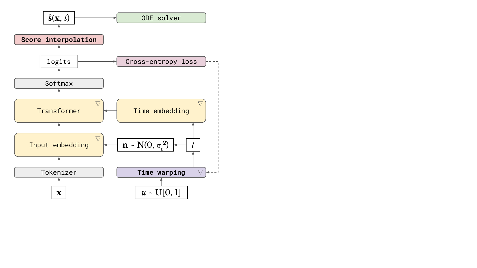
• We describe CDCD, a framework for continuous diffusion models of categorical data (see Figure 1), and explore its application to language modelling and machine translation.

2. Diffusion models

Section Summary: Diffusion models are a way to create new data, like images or text, by starting with random noise and gradually removing it step by step to reveal meaningful patterns, which is easier than trying to generate everything at once like in other AI methods. They work by first mathematically describing a process that corrupts clean data into simple noise, often using equations involving time and random fluctuations, and then training a model to reverse this by predicting and subtracting the noise at each stage. For handling discrete data such as words, the approach embeds it into a continuous space to better manage uncertainty during generation, avoiding early commitments to specific choices that could lead to errors.

Diffusion models enable generative modelling via iterative denoising. Given a gradual corruption process which turns the data distribution into a simple distribution that is easy to sample from (usually an isotropic Gaussian distribution), we can train a model that learns to revert this process step by step. Each step in the reverse direction attempts to reconstruct a small amount of information that the corruption process removed. This is a much easier task than learning to generate data in a single forward pass through a model, as variational autoencoders (VAEs, [26, 27]) and generative adversarial networks (GANs, [28]) do. Autoregressive models similarly enable decomposition of the generative modelling problem into smaller subproblems that are easier to solve. Both of these approaches to iterative refinement are compared in § 2.3.

2.1 Formalism

Many different formalisms have been proposed for diffusion models, e.g. based on score matching ([9]) or latent variable models ([10]). In this work, we will follow [29] and use differential equations to describe the corruption process, as well as the reverse process. We believe that all these different perspectives are largely interchangeable and complementary to some degree.

[29] suggest modelling a diffusion process with the following stochastic differential equation (SDE):

$ \mathrm{d} \mathbf{x} = \mathbf{f}(\mathbf{x}, t) \mathrm{d}t + g(t) \mathrm{d} \mathbf{w},\tag{1} $

where $\mathbf{w}$ is the standard Wiener process, $\mathbf{f}$ is the (vector-valued) drift coefficient, $g$ is the diffusion coefficient and time $t$ ranges from $0$ (clean data) to $T$ (fully corrupted). The reverse process can then be described by the following SDE:

$ \mathrm{d} \mathbf{x} = \left(\mathbf{f}(\mathbf{x}, t) - g(t)^2 \nabla_\mathbf{x} \log p_t(\mathbf{x}) \right)\mathrm{d}t + g(t) \mathrm{d} \mathbf{\bar{w}},\tag{2} $

where $\mathbf{\bar{w}}$ is the standard Wiener process in reversed time. $\mathbf{s}(\mathbf{x}, t) := \nabla_\mathbf{x} \log p_t(\mathbf{x})$ is the so-called score function, i.e. the gradient of the density of $\mathbf{x}$ at time $t$. We can train a model to predict this quantity given $\mathbf{x}$ and $t$ using score matching ([30]):

$ \min \left(\hat{\mathbf{s}}(\mathbf{x}, t) - \nabla_\mathbf{x} \log p_t(\mathbf{x})\right)^2 .\tag{3} $

The estimate $\hat{\mathbf{s}}(\mathbf{x}, t)$ can then be plugged into this SDE to produce samples[^3].

[^3]: We use denoising score matching in practice ([31]).

It turns out that we can instead describe the evolution of $\mathbf{x}$ over time deterministically with an ordinary differential equation (ODE):

$ \mathrm{d} \mathbf{x} = \left(\mathbf{f}(\mathbf{x}, t) - \frac{1}{2} g(t)^2 \nabla_\mathbf{x} \log p_t(\mathbf{x}) \right)\mathrm{d}t.\tag{4} $

This is the probability flow ODE, which has the same marginals $p_t(\mathbf{x})$ as the forward SDE at all timesteps $t$. This equivalence is quite powerful, because it enables us to deterministically map data examples $\mathbf{x}_0$ to latent representations $\mathbf{x}_T$, and vice versa (with $\mathbf{x}_T$ approximately following a Gaussian distribution).

[20] thoroughly explored the design space of diffusion models based on the probability flow ODE formulation, and we will largely follow their recommendations here. Concretely, we will choose $\mathbf{f}(\mathbf{x}, t) = 0$ and $g(t) = \sqrt{2t}$, which yields:

$ \mathrm{d} \mathbf{x} = -t \nabla_\mathbf{x} \log p_t(\mathbf{x}) \mathrm{d}t.\tag{5} $

In this formulation, $t$ corresponds directly to the standard deviation of the Gaussian noise that is added to $\mathbf{x}_0$ to simulate samples from $p_t(\mathbf{x})$ (and therefore they refer to $t$ as $\sigma$ instead[^4]).

[^4]: See Appendix B.1 of [20].

2.2 Diffusion for discrete data

When $\mathbf{x}$ is discrete, the score function is undefined. This can be worked around in two ways: we can try to define a similar iterative refinement procedure through denoising for discrete data, or we can embed $\mathbf{x}$ into a continuous space and apply continuous diffusion to the embeddings. While most of the literature has focused on the former approach (see § 5.1 for an overview), in this work we will explore the latter – abandoning continuity of the input usually means that we have to forgo a lot of useful capabilities, such as classifier-free guidance, which we would like to keep.

Another potential advantage of lifting the discrete input into a continuous space is that it becomes possible to represent superpositions of possible outcomes at intermediate timesteps of the sampling process. In language modelling, this means that we can represent uncertainty at the individual token level: the sampling procedure only commits to specific tokens at the very end. Denoising models that operate directly in the discrete input space do not have this ability: they are only able to represent specific tokens, or the absence of a decision (through use of a 'mask' token). This requirement to commit early to some subset of tokens can lead to inconsistencies in the resulting samples, which are difficult to correct retroactively[^5].

[^5]: Some approaches attempt to mitigate this by allowing some proportion of tokens to be resampled multiple times ([15]).

Changing the input representation to be continuous enables us to use the standard diffusion framework that has been exceptionally successful for perceptual modalities, but we should not necessarily expect it to work as well for language modelling out of the box. In fact, the most commonly used modelling setup for images implicitly reduces the loss weighting of high frequency content relative to likelihood-based models, allowing for a more efficient use of model capacity which is well aligned with human perception ([32]). Furthermore, the underlying physical phenomena that are being modelled (e.g. light intensity, air pressure) are inherently continuous. The relative ease with which diffusion models of images have been scaled to high resolution inputs can at least partially be attributed to these facts. We cannot expect to benefit from this for language modelling, as the notion of `high frequency content' is not meaningful in this setting[^6]. Finally, we also need to consider the impact of the choice of embedding procedure on generative modelling performance.

[^6]: At least, not in the traditional sense; [33] suggest an approach to obtain and analyse multi-scale representations of language.

2.3 Diffusion and autoregression

Autoregressive (AR) models currently dominate language modelling research at scale. They factorise the joint distribution over a token sequence $p(x_1, x_2, ..., x_N)$ into sequential conditionals $p(x_k|x_1, ..., x_{k-1})$ and model each of them separately (with shared parameters). This means sampling always proceeds along the direction of the sequence (i.e. from left to right, when modelling text in English), and in this case, sampling an additional token constitutes an `iterative refinement' step. Autoregression is a very natural fit for language, because it is best represented as a one-dimensional sequence of tokens. That said, the way humans tend to produce language, especially in written form, is far from linear. For many tasks, the ability to go back and refine earlier parts of the sequence, or to construct it hierarchically, is useful.

Changing the modelling paradigm to a more flexible form of iterative refinement (such as diffusion) is desirable, because the increased flexibility would facilitate new applications and could potentially reduce the computational cost of sampling. However, this is a challenging prospect because of the statistical efficiency of AR model training. Because the same parameters can be used to model all sequential conditionals, each training example provides a useful gradient signal for every step of the iterative refinement procedure. This is not the case for diffusion models, where we can only train on a single noise level for each training example. As a result, diffusion models are likely to be less data-efficient, and will converge more slowly. AR models are also able to benefit from caching of previous model activations at sampling time, which significantly reduces the computational cost of each step. Diffusion models require a full forward pass across the entire sequence at each step, which can be much more costly.

Nonetheless, this apparent efficiency benefit of AR models does impose a rather strict constraint on the connectivity patterns within these models – specifically, causality with respect to the input sequence. This constraint is usually implemented using some form of masking, which implies that a significant amount of computation is wasted during training. It also complicates the use of multiresolution architectures, which is very common in other domains of machine learning (e.g. computer vision). Diffusion models on the other hand are completely architecturally unrestricted, so the use of multiresolution architectures (or more exotic variants) is straightforward.

This architectural flexibility compounds with the adaptivity of the denoising procedure, which enables trading off the computational cost and sample quality at sampling time by choosing the appropriate number of iterative refinement steps, without requiring retraining or finetuning. Conversely, for AR models, the number of steps is necessarily the same as the length of the sequence to be generated[^7]. More sophisticated sampling procedures for diffusion models are also being developed on a regular basis, which can be applied to existing models without any changes. Therefore, we believe that diffusion models for language are a worthwhile pursuit, despite their relatively reduced data efficiency.

[^7]: Strictly speaking, it is possible to decouple the cost of sampling from the sequence length even for autoregressive models, using probability density distillation ([34]) or alternative sampling algorithms ([35, 36]), but these approaches have not been used for language models, to the best of our knowledge.

3. The CDCD framework

Section Summary: The CDCD framework enables training diffusion models on categorical data, like words or labels, by adapting familiar techniques to handle discrete inputs in a continuous way. It starts with score interpolation, which uses a simple cross-entropy loss—similar to training language models—to estimate scores by blending predictions of possible data categories, and progresses to jointly learning continuous embeddings for those categories alongside the model itself, using normalization to keep the embeddings stable and distinct. Finally, it incorporates time warping, a method that smartly adjusts the noise added during training to improve efficiency, all visualized in a diagram for clarity.

We will first describe how we can train diffusion models using the familiar categorical cross-entropy loss with score interpolation. We then show how to map categorical inputs to continuous embeddings in a way that is amenable to diffusion, which we achieve by jointly learning the embeddings and the diffusion model itself, allowing them to co-adapt. Finally, we will discuss time warping, an active learning strategy which automatically adapts the distribution of noise levels sampled during training. Together, these components constitute a framework for continuous diffusion of categorical data, or CDCD, which is summarised in a diagram in Figure 1.

3.1 Score interpolation

Diffusion models are typically trained by minimising the score matching objective Equation (3), where the model learns to approximate the score function $\mathbf{s}(\mathbf{x}, t)$ in the least-squares sense. The model predictions can then be substituted directly into Equations 2 or 4 for sampling.

We observe that when the data is discrete and categorical, with tokens taken from a vocabulary of size $V$, the conditional score function $\mathbf{s}(\mathbf{x}, t | \mathbf{x}_0)$ can only assume $V$ possible values. Therefore, if we have a probabilistic prediction of $\mathbf{x}_0$, we can use it to linearly interpolate the $V$ possible values to obtain a score function estimate:

$ \hat{\mathbf{s}}(\mathbf{x}, t) = \sum_{i=1}^V p(\mathbf{x}_0 = \mathbf{e}_i | \mathbf{x}, t) \mathbf{s}(\mathbf{x}, t | \mathbf{x}_0 = \mathbf{e}_i), $

where we have used $\mathbf{e}i$ to represent the embedding corresponding to token $i$ in the vocabulary. Note that this is also equivalent to the expectation $\mathbb{E}{p(\mathbf{x}_0 | \mathbf{x}, t)}\left[\mathbf{s}(\mathbf{x}, t | \mathbf{x}_0) \right]$, which helps explain why this approach works: this expectation is also the minimiser of the score matching loss, so the global optimum is the same for score matching and score interpolation.

To obtain an estimate of $p(\mathbf{x}_0 | \mathbf{x}, t)$, we can make our model predict $V$ logits and apply a softmax nonlinearity, and minimise the categorical cross-entropy loss. This is also the standard setup used to train autoregressive language models (as well as classifiers in general), so it is well-studied and understood, and it ensures stability during training. Compared to the score matching loss, the cross-entropy loss will of course weight errors in the score function estimates differently relative to each other. This difference is important in practice, because we are only able to optimise the loss approximately (i.e. the global optimum is unlikely to be reached), and the relative weighting of the noise levels will also be different.

The conditional score function corresponding to the ODE in Equation 5 is given by:

$ \mathbf{s}(\mathbf{x}, t | \mathbf{x}_0) = \frac{\mathbf{x}_0 - \mathbf{x}}{t^2}, $

which is affine in $\mathbf{x}0$ ([20]). Therefore, the expectation $\mathbb{E}{p(\mathbf{x}_0 | \mathbf{x}, t)}\left[\mathbf{s}(\mathbf{x}, t | \mathbf{x}_0) \right]$ can be written as an affine function of the expectation of $\mathbf{x}_0$ itself:

$ \hat{\mathbf{s}}(\mathbf{x}, t) = \frac{\mathbb{E}_{p(\mathbf{x}_0 | \mathbf{x}, t)}\left[\mathbf{x}_0\right] - \mathbf{x}}{t^2}. $

In other words, we can first obtain an estimate of the ground truth embedding vector $\hat{\mathbf{x}}0 := \mathbb{E}{p(\mathbf{x}_0 | \mathbf{x}, t)}\left[\mathbf{x}_0\right]$, and then use this to obtain a score estimate. This perspective facilitates further modifications to the score estimate, which we will discuss in § 3.2.

3.2 Diffusion on embeddings

To embed the input in a continuous space, we could arbitrarily assign embeddings to different tokens, or use a representation learning technique to obtain embeddings ([18]). However, since we are able to backpropagate gradients from the diffusion model into the embeddings using the reparameterisation trick ([26, 27]), we explore learning the embeddings and the diffusion model jointly. This yields a simpler setup, with a single shared loss function for all model parameters.

If we were to train our diffusion model with score matching, joint training would result in collapse of the embedding space. Since the model is effectively predicting the noise that is added to the embeddings, this task becomes trivial when all embeddings correspond to the same vector. This minimises the loss function, but it does not yield a useful model. Therefore, additional loss terms are necessary to prevent collapse ([17]).

Using score interpolation, we can train the diffusion model with the cross-entropy loss instead. Since the objective is now to distinguish the true embedding from all other embeddings, given a noisy embedding as input, the model is encouraged to push the embeddings as far apart as possible (as this minimises the confounding impact of the noise). We now have the opposite problem, where joint training leads to uncontrollable growth of the embedding parameters, unless they are constrained in some way.

We could again implement such a constraint using additional loss terms, but a simpler alternative is to explicitly normalise the embedding vectors. We find that this approach is very effective, and it yields a model that is trainable end-to-end with the cross-entropy loss, without requiring any additional terms. Concretely, we always L2-normalise the embedding vectors before they are used, but we allow the underlying parameters to vary freely. We backpropagate through the normalisation operation as needed.

We can also apply L2-normalisation to the embedding estimate $\hat{\mathbf{x}}0$ (see § 3.1) before calculating the score estimate, which we refer to as renormalisation. This means that the score estimate no longer corresponds directly to the expectation $\mathbb{E}{p(\mathbf{x}_0 | \mathbf{x}, t)}\left[\mathbf{s}(\mathbf{x}, t | \mathbf{x}_0) \right]$, but rather a rescaled version of it[^8]. Another possible manipulation is to clamp $\hat{\mathbf{x}}_0$ to the nearest embedding vector in the vocabulary (in the Euclidean sense). In practice, we found both of these manipulations to work less well (see § 6.3) – unlike [17], who found that clamping improved their results.

[^8]: We note that L2-normalisation of the expectation resembles the calculation of the mean direction of a von Mises-Fisher distribution.

3.3 Time warping

Diffusion models are essentially denoisers that can operate at many different noise levels with a single set of shared parameters. Therefore, the degree to which the model dedicates capacity to different noise levels has a significant impact on the perceived quality of the resulting samples. We can control this by appropriately weighting the noise levels during training. The impact of different weightings has been studied extensively for diffusion models of images ([37, 32, 38, 20]).

We note that our use of the cross-entropy loss, while conveying many benefits (such as stability and end-to-end training), also changes the relative weighting of the noise levels corresponding to different timesteps $t$. Because the effects of this change are difficult to quantify, we seek to determine a time reweighting strategy that maximises sample quality. In practice, this is best implemented through importance sampling: rather than explicitly multiplying loss contributions from different noise levels with a weighting function $\lambda(t)$, we will instead sample $t$ from a non-uniform distribution, whose density directly corresponds to the desired relative weighting. This way, we avoid introducing significant variance in the loss estimates for timesteps $t$ for which $\lambda(t)$ is particularly large.

To sample $t$ non-uniformly in practice, we can use inverse transform sampling: we first sample uniform samples $u \in [0, 1]$ and then warp them using the inverse cumulative distribution function (CDF) of the distribution which corresponds to the desired weighting: $t = F^{-1}(u)$. This time warping procedure is equivalent to time reweighting in expectation, but more statistically efficient.

To estimate the CDF $F(t)$ in question, we propose to use the following heuristic:

The entropy of the model predictions should increase linearly as a function of $F(t)$.

This heuristic has an intuitive interpretation: it implies that the uncertainty of the model predictions (measured in bits or nats) increases at a constant rate as a function of `uniform time' $u$. Therefore, the capacity of the model should be evenly distributed across the information content of the input sequences. Furthermore, when sampling from the model, using equally spaced timesteps in uniform time will result in a gradual decrease of uncertainty with an approximately constant rate. This ensures that all sampling steps do an equal amount of work in terms of resolving uncertainty.

In practice, we can use the cross-entropy loss values already computed during training as a stand-in for the prediction entropy[^9]. This means we can fit an unnormalised monotonic function $\tilde{F}(t)$ to the observed cross-entropy loss values $\mathcal{L}(t)$ (using the mean squared error loss), which we then need to normalise and invert to implement time warping:

[^9]: In the limit of a model that perfectly approximates the data distribution, the prediction entropy and the cross-entropy should be the same in expectation. In practice, this is a good enough approximation even for undertrained models.

$ \min \left(\tilde{F}(t) - \mathcal{L}(t)\right)^2. $

This yields an active learning strategy where noise levels are initially sampled uniformly, but as training progresses, the noise level distribution changes to focus attention towards those levels for which training is the most useful.

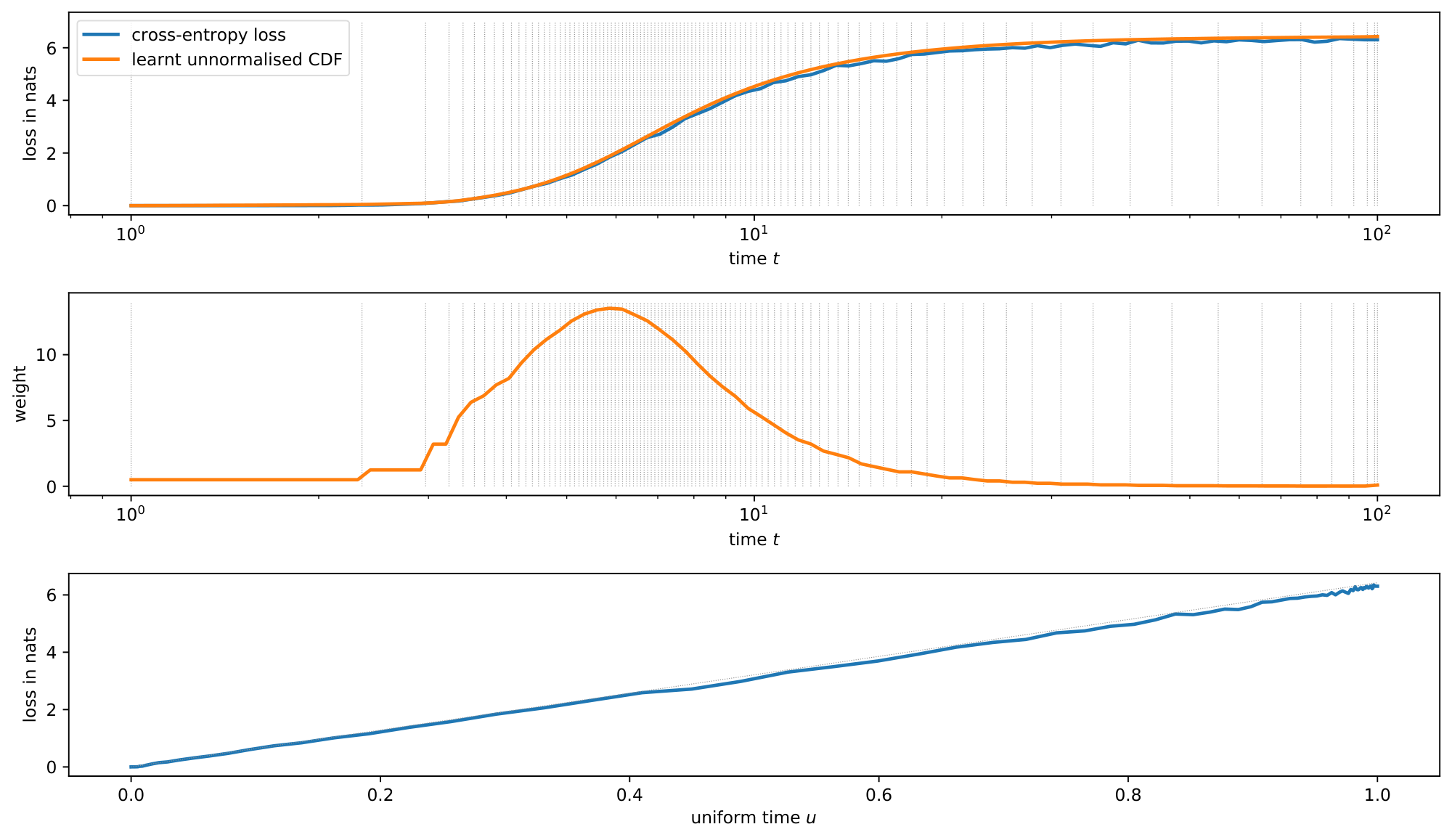
Inspired by [39, 40] we parameterise $\tilde{F}(t)$ as a monotonic piecewise linear function, which is very straightforward to normalise and invert. We describe the fitting procedure in detail in Appendix A. Figure 2 shows the cross-entropy loss as a function of $t$ for a fully trained model, along with the monotonic piecewise linear approximation $\tilde{F}(t)$ (top). It also shows the implied relative weighting of timesteps (middle) and the cross-entropy loss as a function of uniform time $u$ (bottom), which is approximately linear as a result of time warping.

Typically, we find that time warping puts most of the weight on intermediate noise levels. At very low noise levels, the denoising classification problem becomes trivial, because the embeddings corresponding to each token are easy to identify. At very high noise levels, the optimal strategy is to predict the marginal distribution of tokens (given the conditioning), which is also relatively straightforward to learn.

4. Diffusion language models

Section Summary: This section explains how to build language models using a diffusion framework with Transformer architectures, focusing on tasks like completing prompts or filling in missing text by adding noise to parts of the input and gradually refining them. A key tool is a simple mask that flags which words are already known (clean) and which need generating (noisy), allowing the model to handle various scenarios, such as starting from a prefix or conditioning on scattered parts of a sentence, through techniques like prefix, random, or mixed masking. It also incorporates a noise level indicator and self-conditioning, where the model reuses its own prior guesses to work more efficiently without starting from scratch each time.

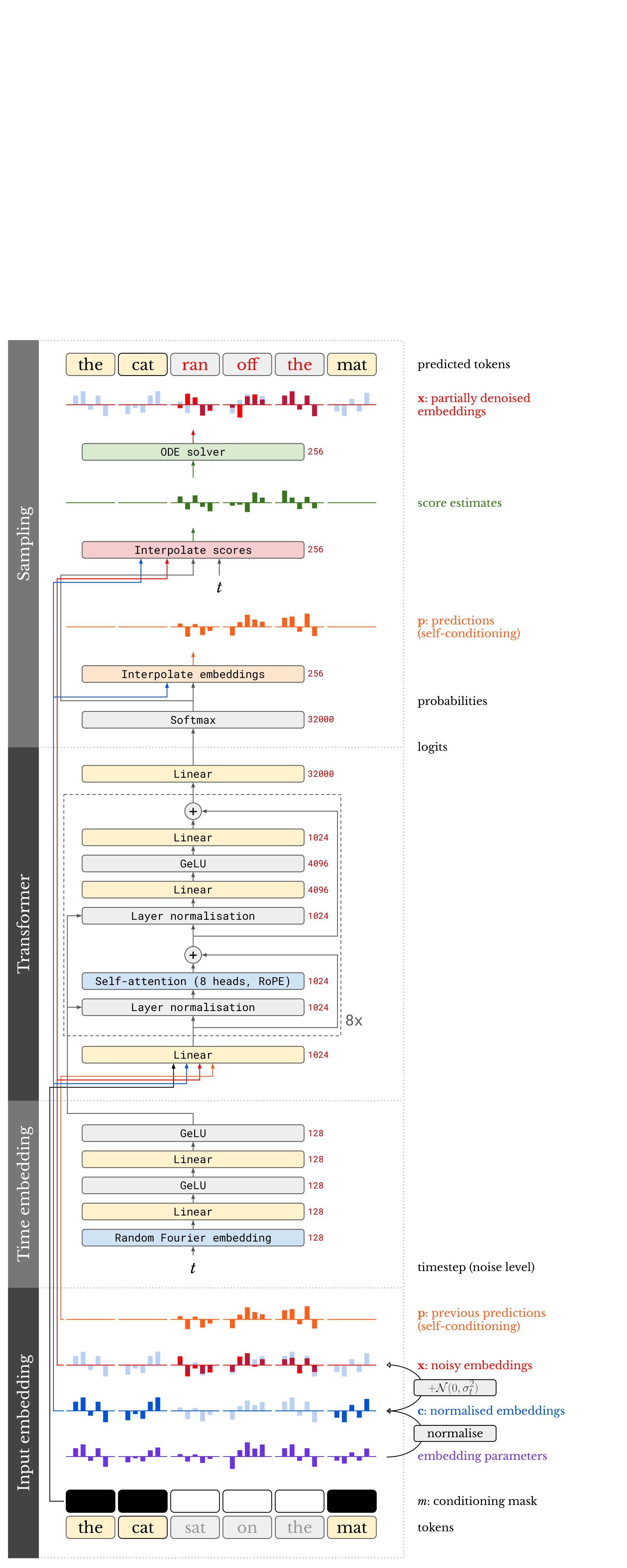
Using the CDCD framework described in the previous section, we can now construct language models for different tasks. We will describe a general Transformer ([7]) architecture which can be used for prompt completion and infilling, using a boolean conditioning mask to indicate which tokens in the sequence are to be sampled ('noisy'), and which tokens are given as conditioning ('clean'). The full model setup is visualised in a diagram in Figure 3. We will also describe an encoder-decoder model architecture for machine translation.

4.1 Mask-conditional Transformer

Since CDCD enables us to reduce the language modelling problem to a denoising classification task, without imposing any restrictions on the model architecture (such as causality, see § 2.3), we are able to use the Transformer architecture without any form of attention masking.

However, practical applications of language modelling require the ability to fix some subset of the tokens in a sequence, while generating the rest, conditioned on these given tokens. One way to achieve this would be to 'clamp' certain token positions throughout the sampling procedure, by reinjecting these tokens at each step, corrupted by the appropriate level of noise. This method was proposed by [29] and referred to as `the replacement method' by [41]. It seems attractive, because it would allow us to treat the model as fully unconditional during training. Nonetheless, it is not as effective as training the model to specifically support conditional sampling out of the box. Indeed, diffusion models for image inpainting are also more effective when trained specifically for that task ([42]).

Therefore, we construct the input to the model by stacking three sequences:

• $\mathbf{x}$: the embeddings corresponding to the noisy input sequence, with embeddings for conditioning tokens set to the zero vector;
• $\mathbf{c}$: the embeddings corresponding to the conditioning tokens, with embeddings for the tokens to be sampled set to the zero vector;
• $m$: the boolean conditioning mask, indicating which tokens are given ('clean', $m_i = 0$) and which are to be generated ('noisy', $m_i = 1$).

As discussed before in § 3.1, the output of the model consists of a sequence of logit vectors, which correspond to the predicted probabilities of each token in the vocabulary occurring at each sequence position. When calculating the training loss, we zero out the positions for given tokens.

Prefix masking

Autoregressive language models naturally allow prefix conditioning, where the start of a sequence is given and the model generates a completion. This is not as straightforward with diffusion models. Since prefix conditioning is a very general procedure for interacting with language models, we would like our models to support it. To achieve this, we randomly sample mask sequences $m$ during training which correspond to prefix conditioning. Such masks consist of a sequence of zeros of a certain length, followed by a sequence of ones, where the length of the prefix is sampled uniformly at random.

Fully random masking

Since diffusion models are able to iteratively refine all tokens in a sequence in parallel, we are not restricted to prefix conditioning. To enable conditioning on an arbitrary subset of sequence positions, we can sample masks $m$ fully randomly during training. Rather than sampling a mask value independently for each sequence position, we first sample a clean position count uniformly at random, and then randomly select a subset of that size from the sequence. This ensures that the model is able to support conditioning on any number of tokens.

Mixed masking

While fully random masking yields the most general model, supporting conditioning on any arbitrary subset of tokens in a sequence, prefix masking is sufficient to support the most common use cases for language models. Somewhat surprisingly, we find that training on an equal mixture of prefix masks and fully random masks actually slightly improves prefix completion performance (see § 6.3).

4.2 Noise level conditioning

Diffusion models operate on inputs corrupted with varying levels of noise. These levels correspond directly to timesteps in the diffusion process. We provide the timestep as an additional input, which is incorporated into the model using conditional normalisation: each layer normalisation operation in the model is followed by shifting and scaling the activations, with the shift and scale parameters depending on the timestep ([43]).

4.3 Self-conditioning

[44] introduced self-conditioning, which significantly improves the performance of diffusion models in certain contexts. They noted that the predictions produced by diffusion models are only used to determine the direction in which to update the noisy input, and are then discarded, which is wasteful. Giving the model direct access to the predictions it produced at the previous sampling step enables a more efficient use of model capacity, by allowing it to refine previous predictions, rather than constructing them from scratch at each step. This approach bears a strong resemblance to the unrolled denoising strategy proposed by [15].

To enable the model to make use of this additional input without requiring unrolling across multiple sampling steps during training, they propose a training procedure which only requires an additional forward pass on half of the batch at each training step. Following [18], we use this procedure and find that it only increases training time by 10-15% for our models in practice, while yielding significant performance gains.

To use self-conditioning with CDCD, the input to the model now consists of four stacked sequences. In addition to $\mathbf{x}$, $\mathbf{c}$ and $m$ (see § 4.1), we add $\mathbf{p}$, which is a sequence of embeddings found by interpolating the vocabulary embeddings using the token probabilities predicted in the previous sampling step (see § 3.1; embeddings for conditioning tokens are set to the zero vector).

4.4 Machine translation model

For machine translation, we use an encoder-decoder architecture with two separate Transformer stacks. Since the conditioning (source) sequence and target sequence are separate, there is no need for masking. We adopt an architecture very similar to the original Transformer ([7]), with absolute positional embeddings (sinusoidal on the source side, learned on the target side) instead of RoPE, and ReLU as activation function.

Generating samples of the correct length is an important concern for translation. As we do not use any causal mask on the decoder side, we cannot simply disregard the contribution to the loss of the positions corresponding to padding tokens during training. Instead, we simply predict the whole sequence of tokens, including beginning-of-sentence (BOS), end-of-sentence (EOS), and padding tokens, up to a constant length. At sampling time, tokens past the first EOS are discarded.

In order to provide a strong conditioning signal to the decoder, we extend the conditioning described in § 4.2 to additionally use the length of the source sequence.

4.5 Comparison to BERT

The model architecture and training procedure we have described so far is very similar to BERT ([21]). Given the widespread use of that model, and its popularity among language modelling practitioners, we provide a side-by-side comparison.

Both models are sequence denoisers, but the nature of the noise differs. While BERT is trained on sequences corrupted by masking noise, which randomly removes a subset of tokens altogether, inputs to our model are corrupted by Gaussian noise which is added directly to the token embeddings. The input consists of a stack of multiple sequences (see § 4.1 and § 4.3), rather than a single sequence where some of the tokens have been masked. Because the intensity of the noise varies according to the timesteps of the diffusion process, we also provide the timestep as an additional input, which is not required for BERT. Finally, to avoid uncontrollable growth of the embedding parameters, we force the embeddings to be normalised. Other than that, the model architectures are essentially identical during training, and the loss functions are the same.

5. Related work

Section Summary: Researchers have developed various diffusion-based methods for refining discrete data like text, shifting from discrete corruption processes—which limit some efficient sampling techniques—to continuous diffusion frameworks applied to discrete inputs through embeddings or relaxations, often targeting language modeling. In machine translation, non-autoregressive iterative refinement models have addressed challenges like inconsistent token predictions by incorporating techniques such as distillation, latent variables, repeated decoding passes, and advanced training procedures in models like CMLM, SMART, Imputer, and DiffusER, narrowing the performance gap with traditional autoregressive approaches while debating their speed benefits. One related study optimizes the noise schedule in diffusion training to reduce loss variance, differing from efforts to align model predictions more linearly.

5.1 Discrete diffusion

Several diffusion-based and diffusion-inspired approaches have been proposed for non-autoregressive iterative refinement of discrete data, and especially for language in particular ([23, 45, 12, 14, 13, 15, 16]). Replacing continuous diffusion with a discrete corruption process affords some flexibility, but it also requires forgoing several capabilities associated with the continuous paradigm, such as efficient sampling algorithms based on advanced ODE solvers, or classifier-free guidance.

More recently, several papers have proposed approaches to apply the continuous diffusion framework to discrete data. It is important to distinguish continuity in the input space from continuity of the time variable of the corruption process; for CDCD, both are continuous. [17], [18] and [46] all target language modelling as the primary application and use an embedding-based strategy in combination with discrete-time diffusion. [47] and [48] propose continuous-time models for discrete input, though they do not explore the application to language modelling. [49] propose concrete score matching, which can be applied to both discrete and continuous inputs. [44] use continuous-time diffusion applied to continuous relaxations of binary representations of the input. [44, 17, 18] also suggested using the cross-entropy loss (in combination with other loss terms).

5.2 Iterative refinement for machine translation

There have been considerable efforts to apply non-autoregressive iterative refinement models to the task of machine translation. The first attempts by [50] already uncovered the issue of 'multi-modality': since non-AR models usually predict all tokens in parallel and independently of each other, uncoordinated sampling decisions might lead to incoherencies like repeated tokens. Earlier advances in sequence-level distillation ([51]) allowed to alleviate those issues, albeit at the cost of expensive training dataset creation. Another line of work introduced a latent transformer ([52]): discrete latents are first sampled autoregressively, and then decoded non-autoregressively.

LVM-DAE ([53]) applied a non-autoregressive decoder multiple times to alleviate multi-modality. Insertion ([54]) and Levenshtein ([55]) transformers demonstrated good parallel decoding results on machine translation along with editing capabilities. The LVM-DAE line of work was later significantly improved upon by the CMLM ([23]) and DisCo ([56]) methods via novel training and decoding procedures. A later work by [57] combined CMLM with local autoregression. Promising advances were achieved by another follow-up of CMLM called SMART ([58]), further closing the gap between AR and non-AR methods. More recently, Imputer ([59, 60]) achieved good results by optimizing alignment between source and target.

[61] questioned the speed advantage of non-AR models in machine translation by comparing them to a shallow-decoder AR baseline. SUNDAE ([15]) introduced step-unrolls and obtained excellent results both in machine translation and unconditional generation without relying on sequence-level distillation. [62] also eliminated distillation with an unroll-like technique. Aggressive decoding ([63]) generated tokens in parallel while using AR models to verify generation and re-generate after the first deviation. DiffusER ([16]) used edit-based reconstructions and 2D beam search to almost completely close the gap between AR and non-AR models in machine translation.

5.3 Other related work

[38] suggest parameterising and optimising the noise schedule during training in a similar fashion to time warping (§ 3.3), though the objective is different: the goal is to minimise the variance of the diffusion loss, whereas our goal is to linearise the entropy of the model predictions.

6. Experiments

Section Summary: In this section, researchers test different design choices for their CDCD language models, comparing them to traditional autoregressive models by training versions for tasks like completing prompts, filling in text gaps, and translating languages. They use a standard transformer architecture with specific settings, such as a 32,000-word vocabulary, noise-added embeddings for training stability, and a mix of masking strategies to handle incomplete text, all optimized over a million steps on diverse web-crawled datasets. Evaluations rely on metrics like translation accuracy scores and measures of text quality and diversity under a reference model, with ablation tests showing that choices like embedding sizes and noise adjustments have minimal impact on performance while techniques like renormalizing predictions improve results.

We study the effect of various design choices, and compare language models based on CDCD with the standard autoregressive approach. We train mask-conditional models for tasks such as prompt completion and infilling, and encoder-decoder models for machine translation.

6.1 Architecture and hyperparameters

For the mask-conditional models, we use a SentencePiece tokenizer ([64]) with a vocabulary size of 32000. We use a standard pre-LN Transformer architecture ([65]) with 8 blocks, 1024 units and rotary positional encodings ([66], RoPE), trained for 1 million steps with batch size 1024 and sequence length 64. We use Random Fourier projections and an MLP with two layers of 128 units to produce timestep embeddings (see Figure 3). We also use self-conditioning ([44]) and time warping. We use 100 bins for the piecewise linear unnormalised CDF $\tilde{F}(t)$ (see § 3.3 and Appendix A).

We set the embedding dimensionality $d = 256$. We L2-normalise the embeddings and scale them by $\sqrt{d}$, so that each component has a standard deviation of 1. We choose $t_{\min} = 1.0$ and $t_{\max} = 300.0$. While these values are quite different from the ones suggested by [20] for image diffusion, we note that the discrete underlying nature of the input data makes it possible to predict the original tokens with 100% accuracy even when noise with $\sigma = 1.0$ is added (recall that $\sigma = t$, see § 2.1). Therefore, it is not useful to consider lower noise levels, except when the embedding dimensionality $d$ is reduced. We scale the noisy embeddings by $\frac{1}{\sqrt{\sigma^2 + \sigma_{data}^2}} = \frac{1}{\sqrt{t^2 + 1}}$ before passing them into the model, so that the components again have a standard deviation of 1.

We drop out the conditioning by zeroing out the corresponding embeddings for 10% of training examples, in order to be able to support sampling with classifier-free guidance ([19]). We use low-discrepancy sampling ([38]) to sample uniform timesteps $u$ before applying time warping, to reduce the variance of the loss estimates. We use a mixed masking strategy (see § 4.1): 50% of the masks sampled during training are prefix masks (with the length of the prefix uniformly sampled), and the other 50% are fully random masks (with the number of clean token positions again uniformly sampled).

We use the Adam optimiser ([67]) with a learning rate of $10^{-4}$, $\beta_1 = 0.9$ and $\beta_2 = 0.99$. We use 200 Euler steps for sampling, and do not tune any sampling parameters (such as temperatures or guidance scales). While this is a large number of steps relative to the sequence length, we wanted to ensure that our measurements would not be negatively affected by discretisation errors introduced by the ODE solver.

6.2 Evaluation

We train mask-conditional models on the MassiveText dataset ([68]), except for the larger model used in § 6.5, which is trained on the publicly available C4 dataset ([69]). Both datasets contain web-crawled content, and are very diverse as a result. For machine translation, we train models on the WMT2014 German-English / English-German and WMT2020 Chinese-English datasets.

To evaluate our machine translation models, we follow the literature and use the BLEU score ([70]). For mask-conditional models, quantitative evaluation is more challenging. Following [15, 18], we measure the likelihood of generated samples under a 1.3B parameter autoregressive language model (AR-NLL), as well as the unigram (per-token) entropy of the samples. As long as the entropy remains high enough, we found this negative log-likelihood to be strongly correlated with subjectively assessed model quality, and we made extensive use of this metric for hyperparameter exploration. To ensure a fair comparison, we always calculate these metrics using a fixed prefix mask with a prefix length of half the sequence length, regardless of the masking strategy used during training.

For experiments with a larger mask-conditional model, we also report the MAUVE metric ([71]), which is specifically designed for open-ended text generation and has been shown to correlate with human judgement (see § 6.5).

6.3 Design decisions

We conduct various ablation experiments to justify our architecture and hyperparameter choices, reporting both the autoregressive negative log likelihood (AR-NLL) and the unigram entropy at the token level (H) in each case. The results are summarised in Table 1 and visualised in Figure 4.

\begin{tabular}{llcc}\toprule
  \multicolumn{2}{l}{\textbf{Ablation}} & \textbf{AR-NLL} & \textbf{Entropy} \\
  \midrule

  \textbf{Base model} & & $\mathbf{4.392_{\pm 0.004}}$ & $\mathbf{7.237_{\pm 0.009}}$ \\
  \midrule
  Data & & $3.389$ & $7.179$ \\
  \midrule

  \multirow{4}{*}{Prediction renormalisation and clamping} & \textbf{neither} & $\mathbf{4.392_{\pm 0.004}}$ & $\mathbf{7.237_{\pm 0.009}}$ \\
  & renormalisation only & $3.762_{\pm 0.003}$ & $6.946_{\pm 0.007}$ \\
  & clamping only & $3.881_{\pm 0.009}$ & $6.770_{\pm 0.020}$ \\
  & both & $3.895_{\pm 0.005}$ & $6.803_{\pm 0.011}$ \\
  \midrule

  \multirow{7}{*}{Embedding dimensionality ($t_{\min} = 0.1$)} & $w=16$ & $4.493_{\pm 0.006}$ & $7.268_{\pm 0.005}$ \\
  & $w=32$ & $4.423_{\pm 0.008}$ & $7.237_{\pm 0.006}$ \\
  & $w=64$ & $4.392_{\pm 0.003}$ & $7.222_{\pm 0.008}$ \\
  & $w=128$ & $4.391_{\pm 0.003}$ & $7.235_{\pm 0.007}$ \\
  & $w=256$ & $4.398_{\pm 0.009}$ & $7.248_{\pm 0.008}$ \\
  & $w=512$ & $4.389_{\pm 0.007}$ & $7.232_{\pm 0.009}$ \\
  & $w=1024$ & $4.386_{\pm 0.004}$ & $7.222_{\pm 0.003}$ \\
  \midrule

  \multirow{5}{*}{Embedding initialisation scale} & $\sigma=0.0001$ & $4.376_{\pm 0.004}$ & $7.226_{\pm 0.006}$ \\
  & $\mathbf{\sigma=0.001}$ & $\mathbf{4.392_{\pm 0.004}}$ & $\mathbf{7.237_{\pm 0.009}}$ \\
  & $\sigma=0.01$ & $4.386_{\pm 0.006}$ & $7.230_{\pm 0.008}$ \\
  & $\sigma=0.1$ & $4.437_{\pm 0.003}$ & $7.257_{\pm 0.003}$ \\
  & $\sigma=1.0$ & $4.617_{\pm 0.002}$ & $7.251_{\pm 0.003}$ \\
  \midrule

  \multirow{6}{*}{Masking strategy} & prefix, fixed length (32) & $4.411_{\pm 0.006}$ & $7.239_{\pm 0.007}$ \\
  & prefix, random length & $4.417_{\pm 0.003}$ & $7.233_{\pm 0.003}$ \\
  & fully random & $4.401_{\pm 0.011}$ & $7.206_{\pm 0.004}$ \\
  & 20\% prefix + 80\% fully random & $4.402_{\pm 0.004}$ & $7.228_{\pm 0.007}$ \\
  & \textbf{50\% prefix + 50\% fully random} & $\mathbf{4.392_{\pm 0.004}}$ & $\mathbf{7.237_{\pm 0.009}}$ \\ 
  & 80\% prefix + 20\% fully random & $4.394_{\pm 0.012}$ & $7.222_{\pm 0.009}$ \\
  \midrule

  \multirow{3}{*}{Self-conditioning (training and sampling)} & neither & $4.781_{\pm 0.010}$ & $7.224_{\pm 0.008}$ \\
  & training only & $4.892_{\pm 0.010}$ & $7.241_{\pm 0.008}$ \\
  & \textbf{both} & $\mathbf{4.392_{\pm 0.004}}$ & $\mathbf{7.237_{\pm 0.009}}$ \\
  \midrule

  \multirow{3}{*}{Time warping (training and sampling)} & neither & $5.091_{\pm 0.007}$ & $7.308_{\pm 0.006}$ \\
  & training only & $5.092_{\pm 0.013}$ & $7.311_{\pm 0.008}$ \\
  & \textbf{both} & $\mathbf{4.392_{\pm 0.004}}$ & $\mathbf{7.237_{\pm 0.009}}$ \\
  \midrule

  \multirow{10}{*}{Time warping: temperature} & $T=0.5$ & $4.445_{\pm 0.006}$ & $7.244_{\pm 0.003}$ \\
  & $T=0.8$ & $4.396_{\pm 0.008}$ & $7.245_{\pm 0.005}$ \\
  & $T=0.9$ & $4.393_{\pm 0.012}$ & $7.235_{\pm 0.011}$ \\
  & $\mathbf{T=1.0}$ & $\mathbf{4.392_{\pm 0.004}}$ & $\mathbf{7.237_{\pm 0.009}}$ \\
  & $T=1.2$ & $4.383_{\pm 0.005}$ & $7.226_{\pm 0.002}$ \\
  & $T=1.5$ & $4.416_{\pm 0.006}$ & $7.251_{\pm 0.007}$ \\
  & $T=2.0$ & $4.442_{\pm 0.006}$ & $7.227_{\pm 0.008}$ \\
  & $T=5.0$ & $4.737_{\pm 0.006}$ & $7.281_{\pm 0.005}$ \\
  & $T=10.0$ & $4.871_{\pm 0.009}$ & $7.275_{\pm 0.006}$ \\
  & $T=100.0$ & $5.036_{\pm 0.007}$ & $7.285_{\pm 0.006}$ \\
  \midrule

  \multirow{8}{*}{Time warping: uniformity} & $\mathbf{\mu=0.0}$ & $\mathbf{4.392_{\pm 0.004}}$ & $\mathbf{7.237_{\pm 0.009}}$ \\
  & $\mu=0.01$ & $4.380_{\pm 0.005}$ & $7.221_{\pm 0.009}$ \\
  & $\mu=0.02$ & $4.381_{\pm 0.006}$ & $7.222_{\pm 0.005}$ \\
  & $\mu=0.05$ & $4.380_{\pm 0.003}$ & $7.235_{\pm 0.005}$ \\
  & $\mu=0.1$ & $4.377_{\pm 0.011}$ & $7.221_{\pm 0.010}$ \\
  & $\mu=0.2$ & $4.419_{\pm 0.005}$ & $7.253_{\pm 0.005}$ \\
  & $\mu=0.5$ & $4.463_{\pm 0.010}$ & $7.249_{\pm 0.006}$ \\
  & $\mu=1.0$ & $5.074_{\pm 0.002}$ & $7.305_{\pm 0.003}$ \\
  \midrule

  \multirow{9}{*}{Time warping: Beta-CDF} & $\alpha=0.5, \beta=0.5$ & $4.364_{\pm 0.005}$ & $7.238_{\pm 0.005}$ \\
  & $\alpha=0.5, \beta=1.0$ & $4.362_{\pm 0.007}$ & $7.224_{\pm 0.008}$ \\
  & $\alpha=0.5, \beta=2.0$ & $4.397_{\pm 0.002}$ & $7.230_{\pm 0.006}$ \\
  & $\alpha=1.0, \beta=0.5$ & $4.449_{\pm 0.007}$ & $7.242_{\pm 0.009}$ \\
  & $\mathbf{\alpha=1.0, \beta=1.0}$ & $\mathbf{4.392_{\pm 0.004}}$ & $\mathbf{7.237_{\pm 0.009}}$ \\
  & $\alpha=1.0, \beta=2.0$ & $4.402_{\pm 0.007}$ & $7.236_{\pm 0.004}$ \\
  & $\alpha=2.0, \beta=0.5$ & $4.544_{\pm 0.011}$ & $7.236_{\pm 0.014}$ \\
  & $\alpha=2.0, \beta=1.0$ & $4.456_{\pm 0.008}$ & $7.238_{\pm 0.009}$ \\
  & $\alpha=2.0, \beta=2.0$ & $4.408_{\pm 0.009}$ & $7.225_{\pm 0.007}$ \\

  \bottomrule
  \end{tabular}

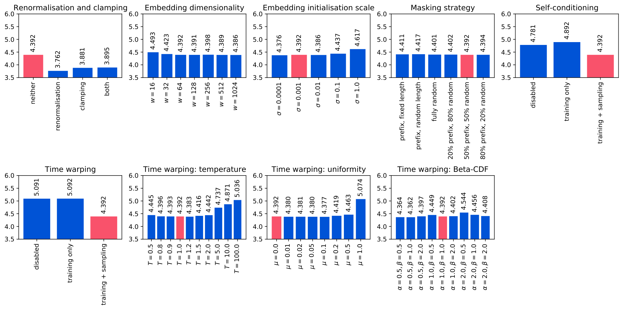
Renormalisation and clamping

Both manipulations of the score estimate (see § 3.2) significantly reduce the AR-NLL, but also reduce the entropy quite a lot. Anecdotally, we also find that models using renormalisation are less amenable to improvements from sampling hyperparameter tuning, and models without renormalisation produce better samples when tuned.

Because we also make use of self-conditioning (see below), it is important to treat renormalisation and clamping as training-time hyperparameters, because they will affect the previous predictions $\mathbf{p}$ that the model receives as input (see § 4.3). When not using self-conditioning, renormalisation and clamping could instead be treated as sampling hyperparameters (see § 6.4).

Embedding dimensionality

We reduced $t_{\min}$ from $1.0$ to $0.1$ for this experiment, because at lower embedding dimensionalities, the same amount of noise erases more information. We verified that the cross-entropy is nearly zero at $t=0.1$ for all values of $w$ we consider[^10]. AR-NLLs initially improve with increasing dimensionality, but stabilise beyond $w=64$, thanks to time warping automatically shifting focus to the relevant noise levels (see Figure 2). We used $w=256$ and $t_{\min}=1.0$ for all other experiments, including the base model, but the result obtained with $t_{\min}=0.1$ is very similar.

[^10]: The cross-entropy is significantly higher than zero at $t=1.0$ for $w=16$, for example.

Embedding initialisation scale

Results degrade when the scale of the initial embedding parameters is too high. We use $\sigma=0.001$ throughout to avoid this pitfall. Given its impact on performance, tuning this parameter is important, which is worth noting because weight initialisation scales are usually chosen heuristically, and generally are not treated as important hyperparameters to tune. We normalise the embeddings whenever they are used (see § 3.2), so the scale of the underlying parameters is not relevant for inference, but clearly it significantly affects optimisation.

Masking strategy

We find that training with fully random masks improves results, even when evaluating using a prefix mask. We suspect that learning the embeddings becomes easier when bidirectional context is available. To ensure that the model uses enough capacity for prefix completion tasks, we use a 50-50 masking strategy for all other experiments.

Self-conditioning

Like [18], we find that self-conditioning ([44]) has a significant positive impact on model performance, by enabling reuse of computation from preceding sampling steps. The AR-NLL improves significantly, while the entropy stays roughly at the same level.

Time warping

During training, focusing on the right noise levels is clearly important, but we also find that spacing the sampling steps accordingly is essential to benefit from this improvement (see § 3.3). We experimented with several manipulations of the warping function to verify the quality of our proposed entropy linearisation heuristic. We find that changing the temperature or the uniformity of the weighting (see Appendix A and Figure 8) can sometimes yield improvements, but they are relatively minor.

Targeting linearity of the loss w.r.t. uniform time $u$ implies an assumption that `all bits are equal', i.e. all information is equally important. To ensure that this is sensible, we also experimented with different target shapes of the loss as a function of $u$. To target a functional shape $S(u): [0, 1] \mapsto [0, 1]$, we minimise $\left(S(F(t)) \frac{\tilde{F}(t)}{F(t)} - \mathcal{L}(t)\right)^2$ instead of $\left(\tilde{F}(t) - \mathcal{L}(t)\right)^2$ to fit the unnormalised CDF ($S$ must be differentiable). Using the CDF of the Beta distribution for $S(u)$, we can produce target shapes with different slopes. We again find only minor improvements by deviating from $\alpha=1.0, \beta=1.0$, which corresponds to the identity function (i.e. targeting a linear shape).

6.4 Sampling

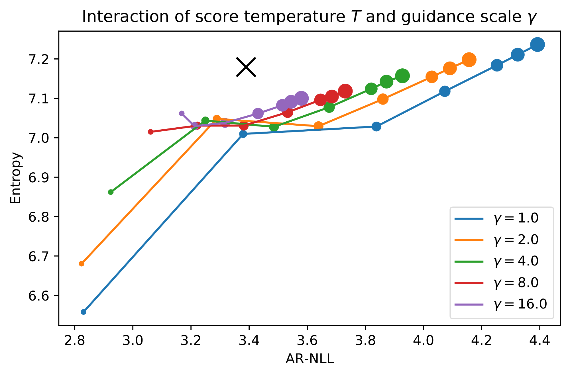
Using the base model, we investigate the impact of various sampling hyperparameters when they are varied individually. Note that there are some significant interactions between sampling hyperparameters, which are not reflected in per-parameter experiments. We will also look at the interaction between the score temperature and the classifier-free guidance scale as an example of this.

\begin{tabular}{llccllcc}\toprule
  \multicolumn{2}{l}{\textbf{Hyperparameter}} & \textbf{AR-NLL} & \textbf{Entropy} & \multicolumn{2}{l}{\textbf{Hyperparameter}} & \textbf{AR-NLL} & \textbf{Entropy}\\
  \cmidrule(lr){1-4}\cmidrule(lr){5-8}

  \textbf{Base model} & & $\mathbf{4.392_{\pm 0.004}}$ & $\mathbf{7.237_{\pm 0.009}}$ & Data & & $3.389$ & $7.179$ \\
  \cmidrule(lr){1-4}\cmidrule(lr){5-8}

  \multirow{6}{2cm}{\# steps (Euler sampler)} & $N=10$ & $5.039_{\pm 0.009}$ & $7.281_{\pm 0.010}$ & \multirow{6}{2cm}{\# steps (Heun sampler)} & $N=5$ & $4.600_{\pm 0.006}$ & $6.955_{\pm 0.009}$ \\
  & $N=20$ & $4.775_{\pm 0.009}$ & $7.270_{\pm 0.010}$ & & $N=10$ & $4.350_{\pm 0.003}$ & $7.044_{\pm 0.007}$ \\
  & $N=50$ & $4.546_{\pm 0.005}$ & $7.249_{\pm 0.008}$ & & $N=25$ & $4.433_{\pm 0.007}$ & $7.196_{\pm 0.008}$ \\
  & $N=100$ & $4.448_{\pm 0.004}$ & $7.241_{\pm 0.008}$ & & $N=50$ & $4.414_{\pm 0.005}$ & $7.227_{\pm 0.008}$ \\
  & $\mathbf{N=200}$ & $\mathbf{4.392_{\pm 0.004}}$ & $\mathbf{7.237_{\pm 0.009}}$ & & $N=100$ & $4.380_{\pm 0.004}$ & $7.231_{\pm 0.008}$ \\
  & $N=500$ & $4.353_{\pm 0.005}$ & $7.231_{\pm 0.009}$ & & $N=250$ & $4.347_{\pm 0.004}$ & $7.229_{\pm 0.008}$ \\
  \cmidrule(lr){1-4}\cmidrule(lr){5-8}

  \multirow{7}{2cm}{Score temperature} & $T=0.5$ & $2.830_{\pm 0.101}$ & $6.558_{\pm 0.102}$ & \multirow{7}{2cm}{Softmax temperature} & $T=0.5$ & $3.743_{\pm 0.004}$ & $6.708_{\pm 0.006}$ \\
  & $T=0.8$ & $3.379_{\pm 0.049}$ & $7.010_{\pm 0.029}$ & & $T=0.8$ & $4.041_{\pm 0.005}$ & $6.999_{\pm 0.006}$ \\
  & $T=0.9$ & $3.838_{\pm 0.010}$ & $7.028_{\pm 0.009}$ & & $T=0.9$ & $4.201_{\pm 0.004}$ & $7.112_{\pm 0.007}$ \\
  & $T=0.95$ & $4.073_{\pm 0.003}$ & $7.118_{\pm 0.008}$ & & $T=0.95$ & $4.294_{\pm 0.003}$ & $7.174_{\pm 0.007}$ \\
  & $T=0.98$ & $4.253_{\pm 0.003}$ & $7.184_{\pm 0.008}$ & & $T=0.98$ & $4.351_{\pm 0.005}$ & $7.211_{\pm 0.008}$ \\
  & $T=0.99$ & $4.324_{\pm 0.003}$ & $7.211_{\pm 0.008}$ & & $T=0.99$ & $4.372_{\pm 0.003}$ & $7.224_{\pm 0.008}$ \\
  & $\mathbf{T=1.0}$ & $\mathbf{4.392_{\pm 0.004}}$ & $\mathbf{7.237_{\pm 0.009}}$ & & $\mathbf{T=1.0}$ & $\mathbf{4.392_{\pm 0.004}}$ & $\mathbf{7.237_{\pm 0.009}}$ \\
  \cmidrule(lr){1-4}\cmidrule(lr){5-8}

  \multirow{7}{2cm}{Initial noise scale} & $\sigma=0.5$ & $3.852_{\pm 0.018}$ & $7.044_{\pm 0.011}$ & \multirow{7}{2cm}{Softmax nucleus} & $p=0.5$ & $3.955_{\pm 0.004}$ & $6.965_{\pm 0.005}$ \\
  & $\sigma=0.8$ & $4.134_{\pm 0.004}$ & $7.137_{\pm 0.008}$ & & $p=0.8$ & $4.217_{\pm 0.005}$ & $7.137_{\pm 0.007}$ \\
  & $\sigma=0.9$ & $4.256_{\pm 0.002}$ & $7.184_{\pm 0.008}$ & & $p=0.9$ & $4.303_{\pm 0.003}$ & $7.188_{\pm 0.007}$ \\
  & $\sigma=0.95$ & $4.325_{\pm 0.003}$ & $7.210_{\pm 0.008}$ & & $p=0.95$ & $4.348_{\pm 0.004}$ & $7.213_{\pm 0.007}$ \\
  & $\sigma=0.98$ & $4.364_{\pm 0.004}$ & $7.226_{\pm 0.008}$ & & $p=0.98$ & $4.374_{\pm 0.004}$ & $7.228_{\pm 0.008}$ \\
  & $\sigma=0.99$ & $4.379_{\pm 0.004}$ & $7.231_{\pm 0.008}$ & & $p=0.99$ & $4.382_{\pm 0.003}$ & $7.233_{\pm 0.008}$ \\
  & $\mathbf{\sigma=1.0}$ & $\mathbf{4.392_{\pm 0.004}}$ & $\mathbf{7.237_{\pm 0.009}}$ & & $p=1.0$ & $\mathbf{4.392_{\pm 0.004}}$ & $\mathbf{7.237_{\pm 0.009}}$ \\
  \cmidrule(lr){1-4}\cmidrule(lr){5-8}

  \multirow{4}{2cm}{Step spacing (no warping)} & $\rho=1.0$ & $5.068_{\pm 0.016}$ & $7.294_{\pm 0.012}$ & \multirow{4}{2cm}{Step spacing (warping)} & $\mathbf{\rho=1.0}$ & $\mathbf{4.392_{\pm 0.004}}$ & $\mathbf{7.237_{\pm 0.009}}$ \\
  & $\rho=2.0$ & $4.631_{\pm 0.005}$ & $7.256_{\pm 0.009}$ & & $\rho=2.0$ & $4.405_{\pm 0.005}$ & $7.240_{\pm 0.009}$ \\
  & $\rho=4.0$ & $4.534_{\pm 0.004}$ & $7.248_{\pm 0.008}$ & & $\rho=4.0$ & $4.424_{\pm 0.005}$ & $7.243_{\pm 0.008}$ \\
  & $\rho=8.0$ & $4.509_{\pm 0.005}$ & $7.246_{\pm 0.009}$ & & $\rho=8.0$ & $4.443_{\pm 0.005}$ & $7.247_{\pm 0.009}$ \\
  \cmidrule(lr){1-4}\cmidrule(lr){5-8}

  \multirow{10}{2cm}{Time warping: temperature} & $T=0.5$ & $4.444_{\pm 0.004}$ & $7.259_{\pm 0.008}$ & \multirow{8}{2cm}{Time warping: uniformity} & $\mathbf{\mu=0.0}$ & $\mathbf{4.392_{\pm 0.004}}$ & $\mathbf{7.237_{\pm 0.009}}$ \\
  & $T=0.8$ & $4.396_{\pm 0.005}$ & $7.239_{\pm 0.009}$ & & $\mu=0.01$ & $4.392_{\pm 0.004}$ & $7.237_{\pm 0.009}$ \\
  & $T=0.9$ & $4.394_{\pm 0.004}$ & $7.238_{\pm 0.009}$ & & $\mu=0.02$ & $4.394_{\pm 0.004}$ & $7.236_{\pm 0.008}$ \\
  & $\mathbf{T=1.0}$ & $\mathbf{4.392_{\pm 0.004}}$ & $\mathbf{7.237_{\pm 0.009}}$ & & $\mu=0.05$ & $4.394_{\pm 0.004}$ & $7.236_{\pm 0.008}$ \\
  & $T=1.2$ & $4.396_{\pm 0.004}$ & $7.236_{\pm 0.008}$ & & $\mu=0.1$ & $4.398_{\pm 0.005}$ & $7.237_{\pm 0.008}$ \\
  & $T=1.5$ & $4.410_{\pm 0.005}$ & $7.237_{\pm 0.008}$ & & $\mu=0.2$ & $4.402_{\pm 0.004}$ & $7.237_{\pm 0.009}$ \\
  & $T=2.0$ & $4.441_{\pm 0.004}$ & $7.238_{\pm 0.008}$ & & $\mu=0.5$ & $4.435_{\pm 0.005}$ & $7.238_{\pm 0.008}$ \\
  & $T=5.0$ & $4.662_{\pm 0.006}$ & $7.255_{\pm 0.009}$ & & $\mu=1.0$ & $5.070_{\pm 0.017}$ & $7.295_{\pm 0.012}$ \\
  & $T=10.0$ & $4.833_{\pm 0.009}$ & $7.269_{\pm 0.011}$ & & & & \\
  & $T=100.0$ & $5.043_{\pm 0.014}$ & $7.291_{\pm 0.011}$ & & & & \\
  \cmidrule(lr){1-4}

  \multirow{5}{2cm}{CF guidance scale} & $\mathbf{\gamma=1.0}$ & $\mathbf{4.392_{\pm 0.004}}$ & $\mathbf{7.237_{\pm 0.009}}$ & & & & \\
  & $\gamma=2.0$ & $4.157_{\pm 0.007}$ & $7.198_{\pm 0.007}$ \\
  & $\gamma=4.0$ & $3.927_{\pm 0.009}$ & $7.157_{\pm 0.007}$ \\
  & $\gamma=8.0$ & $3.731_{\pm 0.005}$ & $7.118_{\pm 0.005}$ \\
  & $\gamma=16.0$ & $3.580_{\pm 0.007}$ & $7.100_{\pm 0.003}$ \\
  \cmidrule(lr){1-4}

  \multirow{2}{2cm}{Final prediction} & disabled & $4.394_{\pm 0.004}$ & $7.237_{\pm 0.009}$ \\
  & \textbf{enabled} & $\mathbf{4.392_{\pm 0.004}}$ & $\mathbf{7.237_{\pm 0.009}}$ \\

  \bottomrule
  \end{tabular}

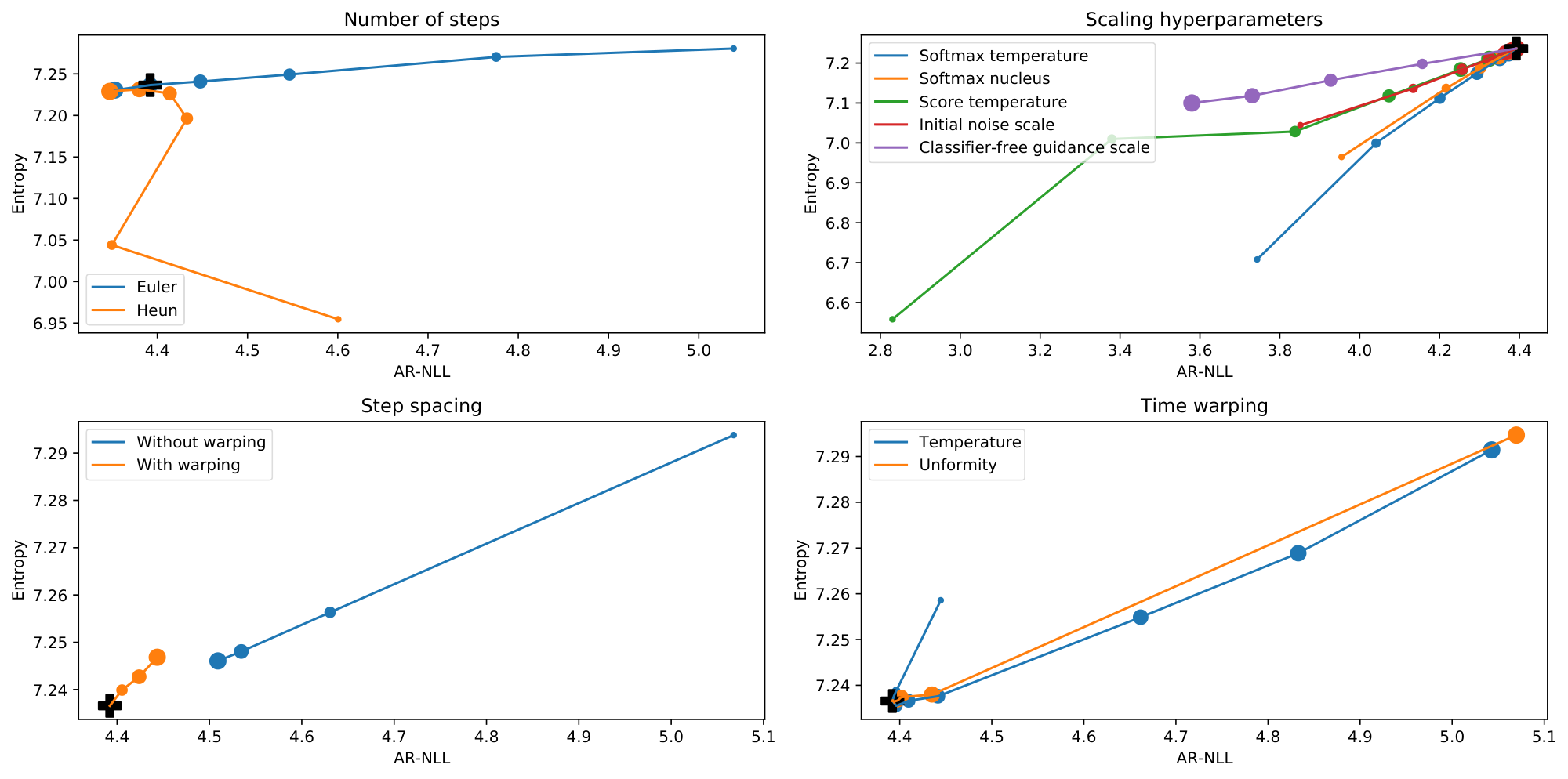
Algorithm and number of steps

We compare the Euler and Heun samplers suggested by [20], reducing the number of sampling steps by a factor of two for the Heun sampler, so that the total number of required function evaluations does not change. For self-conditioning, we always use the most recent model prediction.

The Heun sampler seems to offer little benefit when using a sufficient number of steps[^11], and entropy degrades when the number of steps is decreased, which is not the case for the Euler sampler. We use the Euler sampler with 200 steps for most experiments, but reasonable quality can be achieved with as few as 50 function evaluations. Based on results in the image domain, it may be possible to reduce this further with stochastic samplers[^12], or more advanced sampling algorithms ([72, 73]).

[^11]: Note that the suitability of higher-order samplers is known to be highly dependent on other sampling hyperparameters such as the guidance scale ([73]).

[^12]: Deterministic samplers have some important benefits over stochastic ones, such as support for manipulations in latent space.

Scaling hyperparameters

Many classes of generative models offer some notion of `temperature tuning'. The CDCD framework is particularly versatile in this regard:

• scaling the score function estimate by a factor corresponds to changing the temperature of $p_t(\mathbf{x})$;
• the standard deviation of the initial noise can be reduced below $1.0$, which is often done for flow-based models ([74]);
• since the model produces a categorical probability distribution $p(\mathbf{x}_0 | \mathbf{x}, t)$, we can also manipulate this using various truncation strategies, such as temperature tuning and nucleus sampling[^1] ([75]);
• classifier-free guidance ([19]) can be used to amplify the influence of the conditioning.

[^1]: Nucleus sampling is a misnomer in this case, because we never actually sample from the categorical distribution, but we can still use the same strategy to shape the logits.

Out of these, we find that scaling the score temperature or changing the initial noise scale offer a strictly better trade-off than manipulating $p(\mathbf{x}_0 | \mathbf{x}, t)$. The effectiveness of changing the score temperature is surprising, because this tends to work very poorly for diffusion-based models in the visual domain. While the trade-off offered by classifier-free guidance seems even better at first glance, in practice we find that samples obtained with high guidance scales tend to contain a lot of repeated phrases. We also study the interaction between the score temperature and the guidance scale (see Figure 6), and find that their effects are complementary to a degree.

Step spacing

[20] suggest that spacing the sampling steps non-uniformly significantly improves sample quality. For CDCD, our use of time warping at sampling time already results in non-uniform step spacing. We compare their heuristic for $\rho = 1, 2, 4$ or $8$ with time warping, and we also investigate whether they compound, by applying time warping to non-uniformly spaced steps obtained using their heuristic.

When not using time warping at sampling time, the heuristic is clearly helpful, but it does not reach the same performance. We also find that the effects do not compound, strengthening our intuition that spacing the steps using time warping is close to optimal, because it makes the rate of decrease of uncertainty approximately constant during sampling.

Time warping

In § 6.3, we established that manipulating the warping function at training time is not particularly helpful. We can also choose to manipulate it only at sampling time, where it can still affect step spacing (but not model training). We again find that these manipulations do not have any meaningful positive effect on sample quality.

Final prediction

We run the model one additional time after all sampling steps are completed, and take the argmax of the predicted distributions at each sequence position to determine the sampled tokens. Instead, we could use the tokens whose embeddings are nearest to the predicted embeddings in the Euclidean sense. This works equally well, so it can save some computation, though this only becomes significant if the number of sampling steps is greatly reduced.

6.5 Prompt completion and infilling

We compare a 1.3B parameter model based on the CDCD framework with a pre-trained autoregressive model with the same architecture (24 Transformer blocks, 2048 units, 16 attention heads). Both models are trained on the C4 dataset for 600,000 steps with 524,288 tokens per batch. Due to the reduced data efficiency of diffusion model training (see § 2.3), it is likely that the CDCD model would benefit more from further training. Relative to the autoregressive model, the CDCD model has some extra learnable parameters in the MLP for timestep embedding, and in an initial linear layer which maps the token embeddings to the Transformer hidden state. The token embeddings themselves on the other hand account for $8\times$ fewer parameters, because we use an embedding dimensionality of $256$ instead of $2048$.

While the autoregressive model was trained with a batch size of 256 and a sequence length of 2048, we trained the CDCD model with a batch size of 2048 and a sequence length of 256 instead. This is partly because at this point, we are not focusing our evaluation on long-range coherence, but also because diffusion model training benefits from larger batch sizes: since noise levels are sampled on a per-sequence basis, a larger batch size yields a lower variance loss estimate. Note that the number of sampling steps is still 200, which is now smaller than the sequence length.

We take 5,000 token sequences of length 256 from the C4 validation set (rejecting shorter sequences and cropping longer ones). For each sequence, we select a random-length prefix to use as the prompt, with prompt lengths varying between 0 and 128 (half the sequence length). We sample from the autoregressive model using these prompts with nucleus sampling, for various values of $p$. We prevent the end-of-sentence (EOS) token from being sampled, to ensure that a full-length sequence is produced every time. This is necessary because the MAUVE metric is calculated on the full sequences, including the prompts, so the presence of shorter sequences would bias the results. We also sample from the CDCD model using the same set of prompts, with different score temperatures ($T$) and classifier-free guidance scales ($\gamma$).

The resulting completions are evaluated by comparing them with the original sequences from the dataset using MAUVE, which we report in Table 3, alongside the AR-NLL (measured with the autoregressive model itself[^13]) and the unigram entropy for the generated sequences. We get favourable MAUVE scores with the CDCD model for several settings of the score temperature $T$ and guidance scale $\gamma$. Note however that the MAUVE scores for the autoregressive samples do not seem to be convex in $p$, and it is unclear to what extent any excessive repetition introduced by increasing the guidance scale is penalised, so these numbers should be interpreted with care. Nevertheless, they provide some evidence that the CDCD model is able to produce compelling samples. Selected prompt completion and infilling samples are shown in Figure 7.

[^13]: These numbers are not directly comparable to those reported in Table 1 and Table 2, which were obtained with a model trained on a different dataset.

\begin{tabular}{lllccc}\toprule
  \multicolumn{3}{l}{\textbf{Model}} & \textbf{MAUVE} & \textbf{AR-NLL} & \textbf{Entropy} \\
  \midrule

  Data & & & $1.000$ & $2.580$ & $7.569$ \\
  \midrule

  \multirow{7}{*}{Autoregressive with nucleus sampling} & $p=0.5$ & & $0.545$ & $1.469$ & $7.095$ \\
  & $p=0.8$ & & $0.900$ & $1.887$ & $7.204$ \\
  & $p=0.9$ & & $\mathbf{0.940}$ & $1.988$ & $7.235$ \\
  & $p=0.95$ & & $0.917$ & $2.016$ & $7.244$ \\
  & $p=0.98$ & & $0.928$ & $2.025$ & $7.241$ \\
  & $p=0.99$ & & $0.931$ & $2.027$ & $7.242$ \\
  & $p=1.0$ & & $0.931$ & $2.029$ & $7.242$ \\
  \midrule

  \multirow{30}{*}{CDCD with classifier-free guidance} & \multirow{4}{*}{$T=0.5$} & $\gamma=1.0$ & $0.006$ & $2.377$ & $6.591$ \\
  & & $\gamma=2.0$ & $0.006$ & $1.830$ & $6.444$ \\
  & & $\gamma=4.0$ & $0.009$ & $1.542$ & $6.532$ \\
  & & $\gamma=8.0$ & $0.013$ & $1.522$ & $6.889$ \\
  \cmidrule{2-6}
  & \multirow{4}{*}{$T=0.8$} & $\gamma=1.0$ & $0.215$ & $3.070$ & $6.726$ \\
  & & $\gamma=2.0$ & $0.523$ & $2.399$ & $7.246$ \\
  & & $\gamma=4.0$ & $0.574$ & $2.073$ & $7.488$ \\
  & & $\gamma=8.0$ & $0.555$ & $1.894$ & $7.597$ \\
  \cmidrule{2-6}
  & \multirow{4}{*}{$T=0.9$} & $\gamma=1.0$ & $0.914$ & $3.130$ & $7.353$ \\
  & & $\gamma=2.0$ & $0.939$ & $2.808$ & $7.433$ \\
  & & $\gamma=4.0$ & $0.928$ & $2.535$ & $7.510$ \\
  & & $\gamma=8.0$ & $0.884$ & $2.309$ & $7.570$ \\
  \cmidrule{2-6}
  & \multirow{4}{*}{$T=0.95$} & $\gamma=1.0$ & $0.927$ & $3.466$ & $7.491$ \\
  & & $\gamma=2.0$ & $\mathbf{0.951}$ & $3.173$ & $7.517$ \\
  & & $\gamma=4.0$ & $\mathbf{0.952}$ & $2.874$ & $7.555$ \\
  & & $\gamma=8.0$ & $0.911$ & $2.614$ & $7.594$ \\
  \cmidrule{2-6}
  & \multirow{4}{*}{$T=0.98$} & $\gamma=1.0$ & $0.907$ & $3.724$ & $7.570$ \\
  & & $\gamma=2.0$ & $0.938$ & $3.443$ & $7.576$ \\
  & & $\gamma=4.0$ & $\mathbf{0.950}$ & $3.125$ & $7.594$ \\
  & & $\gamma=8.0$ & $\mathbf{0.947}$ & $2.829$ & $7.613$ \\
  \cmidrule{2-6}
  & \multirow{4}{*}{$T=0.99$} & $\gamma=1.0$ & $0.913$ & $3.821$ & $7.595$ \\
  & & $\gamma=2.0$ & $0.925$ & $3.539$ & $7.597$ \\
  & & $\gamma=4.0$ & $\mathbf{0.953}$ & $3.217$ & $7.607$ \\
  & & $\gamma=8.0$ & $\mathbf{0.943}$ & $2.906$ & $7.621$ \\
  \cmidrule{2-6}
  & \multirow{4}{*}{$T=1.0$} & $\gamma=1.0$ & $0.889$ & $3.926$ & $7.620$ \\
  & & $\gamma=2.0$ & $0.917$ & $3.639$ & $7.618$ \\
  & & $\gamma=4.0$ & $\mathbf{0.949}$ & $3.312$ & $7.623$ \\
  & & $\gamma=8.0$ & $0.937$ & $2.986$ & $7.633$ \\

  \bottomrule
  \end{tabular}

6.6 Machine translation

We compare a Transformer autoregressive machine translation model to a CDCD model with an encoder-decoder of the same size, on three translation tasks – WMT 2014 English-German, WMT 2014 German-English, and WMT 2020 Chinese-English – and two model sizes – Transformer base and big. For each task, all models are trained on the same training set of the corresponding year, and evaluated on newstest2014 and newstest2020 accordingly. The standard validation sets are used for early stopping and for tuning the hyperparameters of CDCD. We train two shared SentencePiece ([64]) tokenizers (one for English/German and one for Chinese/English) of size 32,768, using the unigram method ([76]), with byte fallback.

For the autoregressive baseline, we use the hyperparameters described by [7], except for the following: we tie the source/target/output embeddings following [77], we use the fixed vocabulary size indicated above, and, for Chinese-English only, we use a beam size of 6, and a length penalty $\alpha = 0.6$. The CDCD models are trained for 2M steps, with a batch size of 512 for base and 1024 for big, and a sequence length of 160. We use the same dropout values as for the autoregressive baseline. At sampling time, we set the score temperature $T=0.8$ and classifier-free guidance scales $\gamma = 4.0$ for English-German and German-English, and $\gamma = 8.0$ for Chinese-English, found using a manual hyperparameter search on the validation sets.

Using a diffusion framework provides a natural way of approximating Minimum Bayes-Risk decoding ([78, 79]) by sampling a number of hypotheses, each from a different initial noise vector, and selecting the one minimizing in expectation a metric of interest, in our case BLEU.

We report BLEU scores computed on the test set for each model, year and language pair, using sacreBLEU[^14] ([80]), in Table 4. Overall, CDCD models perform worse (between 3 and 7 BLEU points) than autoregressive counterparts of the same size. The difference is largest on English-German, where manual examination of the samples reveals that hypotheses in English sometimes appear, even though German output is expected. This certainly contributes to the poor score that the CDCD model obtains on this pair. It might be explained by the noisy character of the training data itself (English appearing on the German side). CDCD does comparatively better on Chinese-English, especially at larger scale, which may enable the model to make use of the larger training set. Finally, sampling-based MBR decoding improves translation quality, and monotonically so as a function of the number of samples, providing a gain of 0.7 to 1.8 BLEU points when using 100 samples compared to a single one.

[^14]: The signature is nrefs:1|case:mixed|eff:no|tok:13a|smooth:exp|version:2.3.1 when English is the target language, and nrefs:1|case:mixed|eff:no|tok:intl|smooth:exp|version:2.3.1 for German.

Nonetheless, hypotheses produced by CDCD in our experiments tend to suffer from systematic defects, in particular repeated or missing tokens. We hypothesise that the model is not trained to recover from these errors, and that data augmentation, in the form of extra padding, or corruption, may prove beneficial. We leave exploring this direction to future work.

\begin{tabular}{llrrr}\toprule
  Size & Model & WMT 2014 EN-DE & WMT 2014 DE-EN & WMT 2020 ZH-EN
  \\\midrule
  \multirow{4}{*}{Transformer base} & Autoregressive & 26.2 & 30.2 & 25.2\\
  & CDCD ($n=1$) & 19.3 & 24.9 & 20.7\\
  & CDCD ($n=10$) & 19.7 & 25.4 & 21.7\\
  & CDCD ($n=100$) & 20.0 & 26.0 & 22.2\\
  \midrule
  \multirow{4}{*}{Transformer big} & Autoregressive & 27.6 & 31.3 & 27.1\\
  & CDCD ($n=1$) & 20.7 & 26.0 & 24.0\\
  & CDCD ($n=10$) & 21.9 & 27.0 & 25.0\\
  & CDCD ($n=100$) & 22.4 & 27.8 & 25.6\\
  \bottomrule
  \end{tabular}

7. Discussion

Section Summary: The authors introduce CDCD, a new framework for generating categorical data like text through a diffusion process that's continuous in both time and input, allowing for training of non-step-by-step language models similar to BERT, with benefits like flexible filling in of missing parts and adjustable sampling speeds that balance quality and speed over traditional step-by-step models. While it has some drawbacks, such as handling varying text lengths, and they stuck to standard Transformer designs for simplicity, they note the framework's flexibility for other architectures and plan to test advanced sampling techniques from image generation. Beyond language, CDCD could apply to any structured data generation, potentially improving tools like image creators by better integrating latent spaces and using time adjustments.

We have proposed CDCD, a framework for diffusion of categorical data that is continuous both in time and input space, which enables training of non-autoregressive language models with a procedure reminiscent of BERT (see § 4.5).

Our proposed approach has some advantages over autoregressive models, such as the ability to perform arbitrary infilling[^15] and a flexible sampling procedure which allows trading off sample quality and compute requirements. It also stands to benefit from diffusion model enhancements such as classifier-free guidance and improved sampling algorithms, and from the ability to deterministically map inputs to latents and vice versa (which we have not explored so far). Some limitations compared to autoregressive models were discussed in § 2.3. An important research question which we have not yet investigated, is how best to handle variable-length output. With autoregression, this is very naturally handled by introducing an end-of-sentence (EOS) token, which the model can predict to indicate that sampling should be halted. Diffusion models on the other hand require a fixed-size 'canvas' which is iteratively refined during sampling, although inserting padding tokens at random during training (and collapsing them after sampling) could allow for some length variation ([18]), and it may also reduce the incidence of repeated tokens in the samples.

[^15]: Infilling is also possible with autoregressive models if they are specifically trained for this task ([81]).

Model architecture

We intentionally limited the degree of architectural exploration in this work, because the choice of architecture is largely orthogonal to the framework we have proposed. We focused on the Transformer as it is currently the canonical language model architecture. Nevertheless, we pointed out the absence of any architectural restrictions in this modelling paradigm (see § 2.3), which considerably simplifies the use of more intricate patterns, such as multi-resolution or Perceiver-based architectures ([82]).

We would also like to explore recent innovations for sampling from diffusion models (e.g. [72, 73]), which have so far been demonstrated chiefly in the image domain, and determine to what extent they improve sampling efficiency in the CDCD framework.

Application domains

While we concentrated our empirical evaluation of the proposed CDCD framework on language tasks, none of its components are specific to language. We expect it to be suitable for any generative modelling problem involving structured categorical data. As an example, we note that latent diffusion models such as Stable Diffusion ([83]) first use VQ-VAE ([84]) or VQ-GAN ([85]) to learn a latent space in which the diffusion process is then applied, by mapping the categorical latents to the continuous embeddings from the vector quantisation bottleneck. While this works well, we hypothesise that fitting new embeddings jointly with the diffusion model could bring further improvements, especially in combination with time warping. Finally, our proposed time warping heuristic may also be useful beyond diffusion models of categorical data.

Acknowledgements

Section Summary: The authors express gratitude to a group of colleagues, including Andy Brock, Bart Chrzaszcz, Noah Constant, and others from the DeepMind team, for their helpful assistance and contributions to the work. They also acknowledge the creators and maintainers of various open-source tools that supported the project, such as Python, NumPy, SciPy, JAX, TensorFlow, the DeepMind JAX Ecosystem, Diffrax, and Matplotlib.

We would like to thank Andy Brock, Bart Chrzaszcz, Noah Constant, Jeff Donahue, Douglas Eck, Dominik Grewe, Jordan Hoffmann, Patrick Kidger, Skanda Koppula, Lena Martens, Katie Millican, Ben Moran, Simon Osindero, Evan Shelhamer, Miloš Stanojević, Federico Vaggi, Björn Winckler, and the wider DeepMind team for their assistance and input.

We are also thankful to the creators and maintainers of the open source software used in this work, including Python ([86]), NumPy ([87]), SciPy ([88]), JAX ([89]), TensorFlow ([90]), the DeepMind JAX Ecosystem ([91]), Diffrax ([92]) and Matplotlib ([93]).

Appendix

Section Summary: This appendix describes a method for fitting an unnormalized cumulative distribution function (CDF) to the expected loss over time in a diffusion model, using a piecewise linear approach that's easy to normalize and reverse. It divides time into bins based on adjustable parameters called logits, allowing the function to match real loss patterns without scaling issues, even for conditional models where entropy varies. Additional techniques include correcting for sampling biases, warping timesteps for efficient training and generation, and tweaking the distribution's "temperature" to refine how noise decreases during the process.

A. Fitting the unnormalised CDF

A.1 Parameterisation

To implement time warping (see § 3.3), we fit a monotonically increasing function to the expected loss at each timestep. It is essential to parameterise this function in a way that is easy to normalise and invert, so we can use it for inverse transform sampling.

We take inspiration from [39, 40] and parameterise this function by dividing both the input and output range into bins. For convenience, we will assume that the normalised CDF maps the interval $[0, 1]$ to $[0, 1]$. In practice, timesteps $t$ range from $t_{\min}$ to $t_{\max}$ (with $t_{\max} > t_{\min} > 0$), but we can simply shift and scale them:

$ t' := \frac{t - t_{\min}}{t_{\max} - t_{\min}} . $

The normalised CDF $u = F(t')$ is then parameterised using two sets of logits $l_n^t$ and $l_n^u$, $n = 1, \ldots, N$. Applying the softmax nonlinearity to both sets yields two partitions of the unit interval, which we use to define $N$ input and output regions. The sizes of the input and output bins are:

$ w_n^t = \mathrm{softmax}_n(l_n^t), w_n^u = \mathrm{softmax}_n(l_n^u) . $

The left edges of the input and output bins are found as the cumulative sum of the sizes of all preceding bins:

$ e_1^t = 0, e_n^t = \sum_{m=1}^{n-1} w_m^t, \forall n > 1, $

and similar for $e_n^u$. The right edges are found by adding the bin sizes to the left edges.

Within each region, the CDF can be evaluated by linearly interpolating the bin edges. The result is a piecewise linear function which is guaranteed to be monotonically increasing. We find that enforcing the minimal bin size to be nonzero helps ensure numerical stability, which we implement by adding a small constant to all bin sizes $w_n^t$ and $w_n^u$, and renormalising. By initialising both sets of logits $l_n^t$ and $l_n^u$ to a constant value, $F(t')$ initially represents the identity function, which is the CDF of the uniform distribution on the unit interval. We use the constant $-\log N$, so that the unnormalised CDF $\tilde{F}(t')$ is in fact normalised at the start of training.

A.2 Fitting without normalisation

We now wish to fit $u = F(t')$ so that it has the same shape as the expected loss as a function of time $t'$. However, $F(t')$ is normalised so that $u \in [0, 1]$, whereas the expected loss will vary between $0$ and $H$, the unigram entropy of the data. For an unconditional diffusion model, we can estimate said entropy remarkably accurately from a single batch of training data, simply by counting the frequencies of all tokens in the vocabulary to estimate the marginal token distribution. We could then use this entropy estimate to scale the loss values to the unit interval. Unfortunately, this does not work for conditional models, because in that case, the unigram entropy varies with the conditioning.

It turns out that we can easily define an unnormalised function $\tilde{F}(t')$ using the same parameterisation: instead of applying the softmax nonlinearity to the output logits $l_n^u$, we can apply the exponential function to find the bin sizes:

$ w_n^t = \mathrm{softmax}_n(l_n^t), w_n^u = \exp(l_n^u) . $

The bin edges are now free to assume any positive real value, rather than being constrained to the unit interval. $\tilde{F}(t')$ can therefore be fit to the observed loss values directly. The result of this is shown in Figure 2 (top) for a fully trained model. To ensure that we fit the expectation of the loss at each timestep, we minimise the mean squared error (MSE) loss with respect to the per-sequence loss values observed during training. Once fit, we can obtain the normalised function $F(t') \propto \tilde{F}(t')$ by applying the softmax nonlinearity to the output logits instead of the exponential function, as before.

A.3 Inverse and derivative

Apart from being trivial to normalise, it is also very easy to invert the learnt CDF, simply by switching the roles of the input and output logits $l_n^t$ and $l_n^u$. We can also easily evaluate the derivative of the CDF (i.e. the probability density function), which is piecewise constant: within each bin, it is equal to the ratio of the output and input bin size, $w_n^u / w_n^t$ (Figure 2, middle).

A.4 Importance weighting

Since we are using this fitting mechanism to change the distribution of sampled timesteps over the course of training, we have created a feedback loop, because the training data for $F(t')$ will itself become biased towards oversampled timesteps over the course of training. To compensate for this, we can use importance weights, which correspond to the reciprocal of the derivative of the CDF (or equivalently, the derivative of the inverse CDF). We take care not to backpropagate gradients through the time warping operation and the importance weights. For additional stability, we use an exponential moving average of the parameters $l_n^t$ and $l_n^u$ when performing the warping, to limit the rate of change of the training distribution, though empirically we have found that this is not strictly necessary.

A.5 Warping sampling timesteps

For sampling, we find that using steps that are linearly spaced in uniform time, and subsequently warped, works considerably better than using uniformly spaced timesteps. Using warping for both training (to change the distribution of noise levels on the fly) and sampling (to space the timesteps nonlinearly) yields the best results. We hypothesise that decreasing the entropy at a constant rate from step to step is also a useful heuristic for sampling.

A.6 Temperature and uniformity

The piecewise linear parameterisation also enables some useful distribution manipulations: we can easily change the temperature $T$ of the distribution represented by the CDF, by changing the output bin sizes:

$ {w'}_n^u \propto w_n^u \cdot \left(\frac{w_n^u}{w_n^t}\right)^{T^{-1} - 1} . $

To see why this corresponds to a temperature change, recall that the PDF is piecewise constant, and the values it assumes (up to a normalisation constant) are given by:

$ \frac{{w'}_n^u}{w_n^t} \propto \frac{w_n^u}{w_n^t} \cdot \left(\frac{w_n^u}{w_n^t}\right)^{T^{-1} - 1} = \left(\frac{w_n^u}{w_n^t}\right)^{T^{-1}}. $

Similarly, we can also derive the CDF of a mixture of the distribution with a uniform distribution, with mixture weight $\mu$:

$ {w''}_n^u = (1 - \mu) \cdot w_n^u + \mu \cdot w_n^t . $

Note that when the corresponding input and output bin sizes are all equal to each other (i.e. $w_n^u = w_n^t, \forall n$), we always obtain the identity function, which corresponds to the CDF of the uniform distribution on the unit interval.

The effect of these manipulations is visualised in Figure 8.

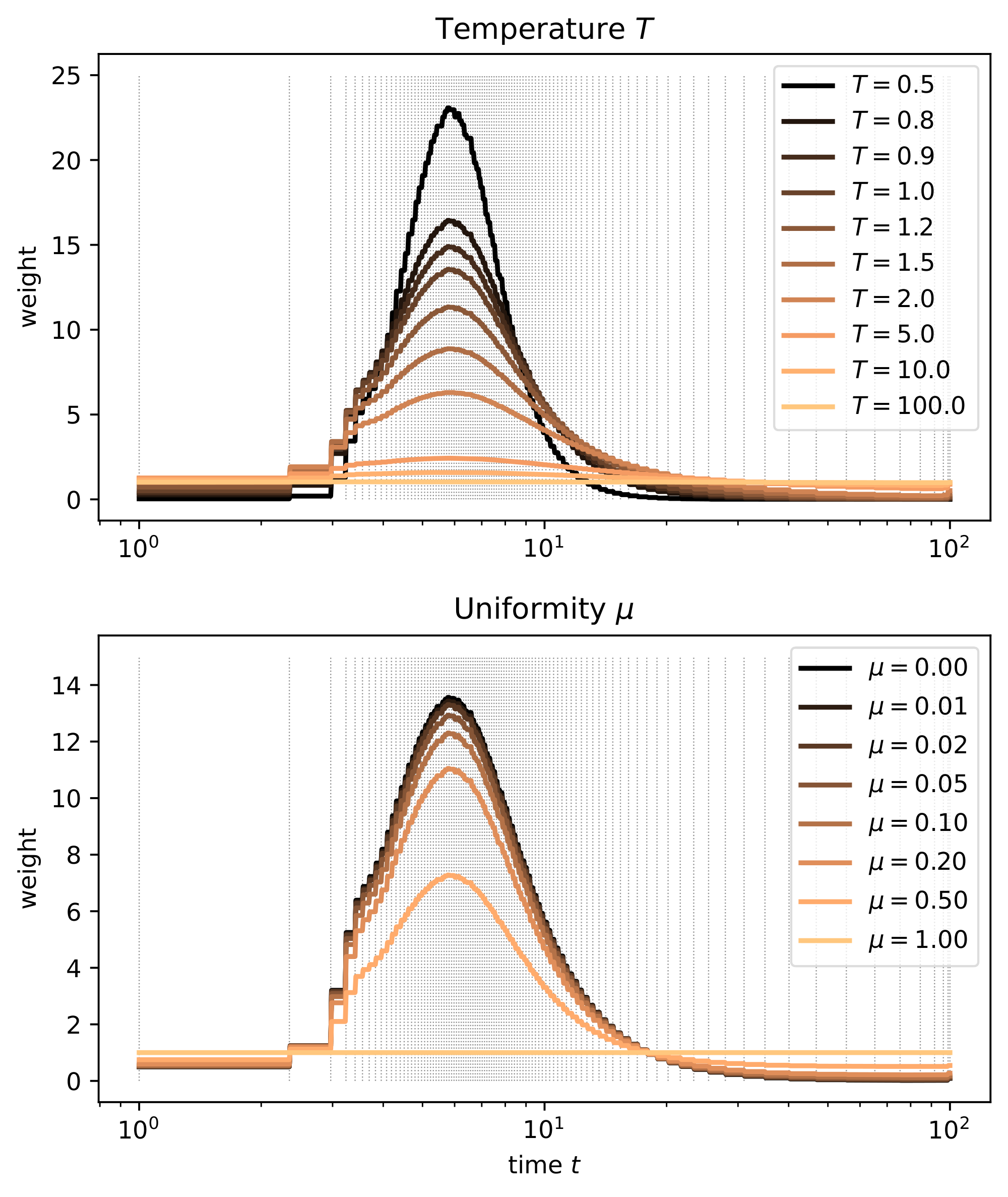
B. Negative results

We informally discuss some failed attempts to improve our results. This information is provided to help understand some of our design choices, and to aid researchers and practitioners who are interested in using these methods or investigating ways to improve them. Bearing in mind that context and details significantly impact experimental results, especially in machine learning research, we expressly do not wish to discourage anyone from pursuing the ideas described here.

B.1 Constraining the embedding parameters

Instead of normalisation, the embedding parameters can also be prevented from growing uncontrollably by adding a regularisation loss term. We experimented with L2 regularisation, margin penalties ([94, 95]), as well as automatic adaptation of the L2 penalty weight to target unit variance for the embedding vector components ([96, 95]), but found that normalisation works best.

B.2 Removing the time dependency

In an effort to simplify the model architecture and make it resemble BERT even more strongly, we investigated models without time embedding (i.e. we removed the time embedding MLP in Figure 3). Since the model is solving a classification task, our hypothesis was that it could simply infer the noise level from the noisy input vectors, instead of requiring explicit knowledge of the timestep $t$. Unfortunately this significantly hurt performance. We suspect that this is a result of the relative scale of the embeddings and the noise (which varies greatly across noise levels), as well as the rescaling we apply to the noisy embeddings to ensure unit variance (see § 6.1).

B.3 Simplex diffusion

We started out by lifting discrete token sequences into the space of categorical distributions over tokens, and performing diffusion in that space. Categorical distributions are nonnegative real-valued vectors whose components sum to 1, so they live on the simplex. We explored a tractable formulation of diffusion on the simplex, based on the Cox-Ingersoll-Ross process ([97]), as described by [98].

We found that language modelling with this process is impeded by the uneven nature of the corruption process, which is a consequence of the high dimensionality of the simplex (corresponding to the number of tokens in the vocabulary $V$). In practice, the noise distribution is heavy-tailed and introduces frequent outliers, which make the corrupted vectors look like they correspond to the wrong tokens, even at very low noise levels. We were not able to circumvent this issue even with powerful Transformer models. We hypothesise that mitigating this issue requires modifying the corruption process so that it does not operate independently on all components. Formulating such a correlated process with a tractable transition density is non-trivial however, and this would complicate the model to a certain degree.

Both score interpolation (§ 3.1) and time warping (§ 3.3) were originally developed in the context of simplex diffusion, but we found these ideas to be more effective in combination with Gaussian diffusion in a Euclidean embedding space.

References

Section Summary: This section provides a bibliography of key research papers in artificial intelligence and machine learning, spanning from 2005 to 2022, that underpin advancements in generative models. It includes foundational works on language models like GPT and BERT, as well as techniques for creating images, audio, video, and text through methods such as diffusion models, variational autoencoders, and generative adversarial networks. These papers, published in prestigious venues like NeurIPS and arXiv, were authored by leading experts and explore how AI can learn and produce content from data patterns.

[1] T. Brown, B. Mann, N. Ryder, M. Subbiah, J. D. Kaplan, P. Dhariwal, A. Neelakantan, P. Shyam, G. Sastry, A. Askell, et al. Language models are few-shot learners. Advances in neural information processing systems, 33:1877–1901, 2020.

[2] P. Dhariwal, H. Jun, C. Payne, J. W. Kim, A. Radford, and I. Sutskever. Jukebox: A generative model for music. arXiv preprint arXiv:2005.00341, 2020.

[3] Z. Borsos, R. Marinier, D. Vincent, E. Kharitonov, O. Pietquin, M. Sharifi, O. Teboul, D. Grangier, M. Tagliasacchi, and N. Zeghidour. AudioLM: a language modeling approach to audio generation. arXiv preprint arXiv:2209.03143, 2022.

[4] A. Ramesh, P. Dhariwal, A. Nichol, C. Chu, and M. Chen. Hierarchical text-conditional image generation with clip latents. arXiv preprint arXiv:2204.06125, 2022.

[5] C. Saharia, W. Chan, S. Saxena, L. Li, J. Whang, E. Denton, S. K. S. Ghasemipour, B. K. Ayan, S. S. Mahdavi, R. G. Lopes, et al. Photorealistic text-to-image diffusion models with deep language understanding. arXiv preprint arXiv:2205.11487, 2022b.

[6] J. Ho, W. Chan, C. Saharia, J. Whang, R. Gao, A. Gritsenko, D. P. Kingma, B. Poole, M. Norouzi, D. J. Fleet, et al. Imagen video: High definition video generation with diffusion models. arXiv preprint arXiv:2210.02303, 2022a.

[7] A. Vaswani, N. Shazeer, N. Parmar, J. Uszkoreit, L. Jones, A. N. Gomez, Ł. Kaiser, and I. Polosukhin. Attention is all you need. Advances in neural information processing systems, 30, 2017.

[8] J. Sohl-Dickstein, E. Weiss, N. Maheswaranathan, and S. Ganguli. Deep unsupervised learning using nonequilibrium thermodynamics. In International Conference on Machine Learning, pages 2256–2265. PMLR, 2015.

[9] Y. Song and S. Ermon. Generative modeling by estimating gradients of the data distribution. Advances in Neural Information Processing Systems, 32, 2019.

[10] J. Ho, A. Jain, and P. Abbeel. Denoising diffusion probabilistic models. Advances in Neural Information Processing Systems, 33:6840–6851, 2020.

[11] J. Yu, Y. Xu, J. Y. Koh, T. Luong, G. Baid, Z. Wang, V. Vasudevan, A. Ku, Y. Yang, B. K. Ayan, et al. Scaling autoregressive models for content-rich text-to-image generation. arXiv preprint arXiv:2206.10789, 2022.

[12] J. Austin, D. D. Johnson, J. Ho, D. Tarlow, and R. van den Berg. Structured denoising diffusion models in discrete state-spaces. Advances in Neural Information Processing Systems, 34:17981–17993, 2021.

[13] E. Hoogeboom, D. Nielsen, P. Jaini, P. Forré, and M. Welling. Argmax flows and multinomial diffusion: Learning categorical distributions. Advances in Neural Information Processing Systems, 34:12454–12465, 2021b.

[14] E. Hoogeboom, A. A. Gritsenko, J. Bastings, B. Poole, R. v. d. Berg, and T. Salimans. Autoregressive diffusion models. arXiv preprint arXiv:2110.02037, 2021a.

[15] N. Savinov, J. Chung, M. Binkowski, E. Elsen, and A. v. d. Oord. Step-unrolled denoising autoencoders for text generation. arXiv preprint arXiv:2112.06749, 2021.

[16] M. Reid, V. J. Hellendoorn, and G. Neubig. Diffuser: Discrete diffusion via edit-based reconstruction, 2022.

[17] X. L. Li, J. Thickstun, I. Gulrajani, P. Liang, and T. B. Hashimoto. Diffusion-lm improves controllable text generation. arXiv preprint arXiv:2205.14217, 2022.

[18] R. Strudel, C. Tallec, F. Altché, Y. Du, Y. Ganin, A. Mensch, W. Grathwohl, N. Savinov, S. Dieleman, L. Sifre, and R. Leblond. Self-conditioned embedding diffusion for text generation, 2022.

[19] J. Ho and T. Salimans. Classifier-free diffusion guidance. arXiv preprint arXiv:2207.12598, 2022.

[20] T. Karras, M. Aittala, T. Aila, and S. Laine. Elucidating the design space of diffusion-based generative models. arXiv preprint arXiv:2206.00364, 2022.

[21] J. Devlin, M.-W. Chang, K. Lee, and K. Toutanova. Bert: Pre-training of deep bidirectional transformers for language understanding. arXiv preprint arXiv:1810.04805, 2018.

[22] A. Wang and K. Cho. Bert has a mouth, and it must speak: Bert as a markov random field language model. In Proceedings of the Workshop on Methods for Optimizing and Evaluating Neural Language Generation, pages 30–36, 2019.

[23] M. Ghazvininejad, O. Levy, Y. Liu, and L. Zettlemoyer. Mask-predict: Parallel decoding of conditional masked language models. In Proceedings of the 2019 Conference on Empirical Methods in Natural Language Processing and the 9th International Joint Conference on Natural Language Processing (EMNLP-IJCNLP), pages 6112–6121, 2019.

[24] K. Goyal, C. Dyer, and T. Berg-Kirkpatrick. Exposing the implicit energy networks behind masked language models via metropolis–hastings. arXiv preprint arXiv:2106.02736, 2021.

[25] A. Shih, D. Sadigh, and S. Ermon. Training and inference on any-order autoregressive models the right way. arXiv preprint arXiv:2205.13554, 2022.

[26] D. P. Kingma and M. Welling. Auto-encoding variational bayes. arXiv preprint arXiv:1312.6114, 2013.

[27] D. J. Rezende, S. Mohamed, and D. Wierstra. Stochastic backpropagation and approximate inference in deep generative models. In International conference on machine learning, pages 1278–1286. PMLR, 2014.

[28] I. Goodfellow, J. Pouget-Abadie, M. Mirza, B. Xu, D. Warde-Farley, S. Ozair, A. Courville, and Y. Bengio. Generative adversarial nets. In Z. Ghahramani, M. Welling, C. Cortes, N. Lawrence, and K. Weinberger, editors, Advances in Neural Information Processing Systems, volume 27. Curran Associates, Inc., 2014.

[29] Y. Song, J. Sohl-Dickstein, D. P. Kingma, A. Kumar, S. Ermon, and B. Poole. Score-based generative modeling through stochastic differential equations. In International Conference on Learning Representations, 2020.

[30] A. Hyvärinen and P. Dayan. Estimation of non-normalized statistical models by score matching. Journal of Machine Learning Research, 6(4), 2005.

[31] P. Vincent. A connection between score matching and denoising autoencoders. Neural computation, 23(7):1661–1674, 2011.

[32] Y. Song, C. Durkan, I. Murray, and S. Ermon. Maximum likelihood training of score-based diffusion models. Advances in Neural Information Processing Systems, 34:1415–1428, 2021a.

[33] A. Tamkin, D. Jurafsky, and N. Goodman. Language through a prism: A spectral approach for multiscale language representations. Advances in Neural Information Processing Systems, 33:5492–5504, 2020.

[34] A. van den Oord, Y. Li, I. Babuschkin, K. Simonyan, O. Vinyals, K. Kavukcuoglu, G. Driessche, E. Lockhart, L. Cobo, F. Stimberg, et al. Parallel wavenet: Fast high-fidelity speech synthesis. In International conference on machine learning, pages 3918–3926. PMLR, 2018.

[35] Y. Song, C. Meng, R. Liao, and S. Ermon. Accelerating feedforward computation via parallel nonlinear equation solving. In International Conference on Machine Learning, pages 9791–9800. PMLR, 2021b.

[36] V. Jayaram and J. Thickstun. Parallel and flexible sampling from autoregressive models via langevin dynamics. In International Conference on Machine Learning, pages 4807–4818. PMLR, 2021.

[37] A. Q. Nichol and P. Dhariwal. Improved denoising diffusion probabilistic models. In International Conference on Machine Learning, pages 8162–8171. PMLR, 2021.

[38] D. Kingma, T. Salimans, B. Poole, and J. Ho. Variational diffusion models. Advances in neural information processing systems, 34:21696–21707, 2021.

[39] T. Müller, B. McWilliams, F. Rousselle, M. Gross, and J. Novák. Neural importance sampling. ACM Transactions on Graphics (TOG), 38(5):1–19, 2019.

[40] C. Durkan, A. Bekasov, I. Murray, and G. Papamakarios. Neural spline flows. Advances in neural information processing systems, 32, 2019.

[41] J. Ho, T. Salimans, A. A. Gritsenko, W. Chan, M. Norouzi, and D. J. Fleet. Video diffusion models. In ICLR Workshop on Deep Generative Models for Highly Structured Data, 2022b.

[42] C. Saharia, W. Chan, H. Chang, C. Lee, J. Ho, T. Salimans, D. Fleet, and M. Norouzi. Palette: Image-to-image diffusion models. In ACM SIGGRAPH 2022 Conference Proceedings, pages 1–10, 2022a.

[43] E. Perez, F. Strub, H. De Vries, V. Dumoulin, and A. Courville. Film: Visual reasoning with a general conditioning layer. In Proceedings of the AAAI Conference on Artificial Intelligence, volume 32, 2018.

[44] T. Chen, R. Zhang, and G. Hinton. Analog bits: Generating discrete data using diffusion models with self-conditioning. arXiv preprint arXiv:2208.04202, 2022.

[45] H. Chang, H. Zhang, L. Jiang, C. Liu, and W. T. Freeman. Maskgit: Masked generative image transformer. In Proceedings of the IEEE/CVF Conference on Computer Vision and Pattern Recognition, pages 11315–11325, 2022.

[46] X. Han, S. Kumar, and Y. Tsvetkov. SSD-LM: Semi-autoregressive simplex-based diffusion language model for text generation and modular control, 2022.

[47] A. Campbell, J. Benton, V. De Bortoli, T. Rainforth, G. Deligiannidis, and A. Doucet. A continuous time framework for discrete denoising models. arXiv preprint arXiv:2205.14987, 2022.

[48] H. Sun, L. Yu, B. Dai, D. Schuurmans, and H. Dai. Score-based continuous-time discrete diffusion models. arXiv preprint arXiv:2211.16750, 2022.

[49] C. Meng, K. Choi, J. Song, and S. Ermon. Concrete score matching: Generalized score matching for discrete data. arXiv preprint arXiv:2211.00802, 2022.

[50] J. Gu, J. Bradbury, C. Xiong, V. O. Li, and R. Socher. Non-autoregressive neural machine translation. arXiv preprint arXiv:1711.02281, 2017.

[51] Y. Kim and A. M. Rush. Sequence-level knowledge distillation. arXiv preprint arXiv:1606.07947, 2016.

[52] L. Kaiser, S. Bengio, A. Roy, A. Vaswani, N. Parmar, J. Uszkoreit, and N. Shazeer. Fast decoding in sequence models using discrete latent variables. In International Conference on Machine Learning, pages 2390–2399. PMLR, 2018.

[53] J. Lee, E. Mansimov, and K. Cho. Deterministic non-autoregressive neural sequence modeling by iterative refinement. arXiv preprint arXiv:1802.06901, 2018.

[54] M. Stern, W. Chan, J. Kiros, and J. Uszkoreit. Insertion transformer: Flexible sequence generation via insertion operations. In International Conference on Machine Learning, pages 5976–5985. PMLR, 2019.

[55] J. Gu, C. Wang, and J. Zhao. Levenshtein transformer. arXiv preprint arXiv:1905.11006, 2019.

[56] J. Kasai, J. Cross, M. Ghazvininejad, and J. Gu. Non-autoregressive machine translation with disentangled context transformer. In International Conference on Machine Learning, pages 5144–5155. PMLR, 2020a.

[57] X. Kong, Z. Zhang, and E. Hovy. Incorporating a local translation mechanism into non-autoregressive translation. arXiv preprint arXiv:2011.06132, 2020.

[58] M. Ghazvininejad, O. Levy, and L. Zettlemoyer. Semi-autoregressive training improves mask-predict decoding. arXiv preprint arXiv:2001.08785, 2020.

[59] W. Chan, C. Saharia, G. Hinton, M. Norouzi, and N. Jaitly. Imputer: Sequence modelling via imputation and dynamic programming. In International Conference on Machine Learning, pages 1403–1413. PMLR, 2020.

[60] C. Saharia, W. Chan, S. Saxena, and M. Norouzi. Non-autoregressive machine translation with latent alignments. arXiv preprint arXiv:2004.07437, 2020.

[61] J. Kasai, N. Pappas, H. Peng, J. Cross, and N. A. Smith. Deep encoder, shallow decoder: Reevaluating non-autoregressive machine translation. arXiv preprint arXiv:2006.10369, 2020b.

[62] X. S. Huang, F. Perez, and M. Volkovs. Improving non-autoregressive translation models without distillation. In International Conference on Learning Representations, 2022.

[63] H. Xia, T. Ge, F. Wei, and Z. Sui. Lossless speedup of autoregressive translation with generalized aggressive decoding. arXiv preprint arXiv:2203.16487, 2022.

[64] T. Kudo and J. Richardson. Sentencepiece: A simple and language independent subword tokenizer and detokenizer for neural text processing. arXiv preprint arXiv:1808.06226, 2018.

[65] R. Xiong, Y. Yang, D. He, K. Zheng, S. Zheng, C. Xing, H. Zhang, Y. Lan, L. Wang, and T. Liu. On layer normalization in the transformer architecture. In International Conference on Machine Learning, pages 10524–10533. PMLR, 2020.

[66] J. Su, Y. Lu, S. Pan, B. Wen, and Y. Liu. Roformer: Enhanced transformer with rotary position embedding. arXiv preprint arXiv:2104.09864, 2021.

[67] D. P. Kingma and J. Ba. Adam: A method for stochastic optimization. In International Conference on Learning Representations, 2015.

[68] J. W. Rae, S. Borgeaud, T. Cai, K. Millican, J. Hoffmann, F. Song, J. Aslanides, S. Henderson, R. Ring, S. Young, et al. Scaling language models: Methods, analysis & insights from training gopher. arXiv preprint arXiv:2112.11446, 2021.

[69] C. Raffel, N. Shazeer, A. Roberts, K. Lee, S. Narang, M. Matena, Y. Zhou, W. Li, and P. J. Liu. Exploring the limits of transfer learning with a unified text-to-text transformer. arXiv e-prints, 2019.

[70] K. Papineni, S. Roukos, T. Ward, and W.-J. Zhu. Bleu: a method for automatic evaluation of machine translation. In Proceedings of the 40th annual meeting of the Association for Computational Linguistics, pages 311–318, 2002.

[71] K. Pillutla, S. Swayamdipta, R. Zellers, J. Thickstun, S. Welleck, Y. Choi, and Z. Harchaoui. Mauve: Measuring the gap between neural text and human text using divergence frontiers. In NeurIPS, 2021.

[72] C. Lu, Y. Zhou, F. Bao, J. Chen, C. Li, and J. Zhu. Dpm-solver: A fast ode solver for diffusion probabilistic model sampling in around 10 steps. arXiv preprint arXiv:2206.00927, 2022a.

[73] C. Lu, Y. Zhou, F. Bao, J. Chen, C. Li, and J. Zhu. Dpm-solver++: Fast solver for guided sampling of diffusion probabilistic models. arXiv preprint arXiv:2211.01095, 2022b.

[74] D. P. Kingma and P. Dhariwal. Glow: Generative flow with invertible 1x1 convolutions. Advances in neural information processing systems, 31, 2018.

[75] A. Holtzman, J. Buys, L. Du, M. Forbes, and Y. Choi. The curious case of neural text degeneration. In International Conference on Learning Representations, 2019.

[76] T. Kudo. Subword regularization: Improving neural network translation models with multiple subword candidates. In Proceedings of the 56th Annual Meeting of the Association for Computational Linguistics (Volume 1: Long Papers), pages 66–75, Melbourne, Australia, July 2018. Association for Computational Linguistics. doi:10.18653/v1/P18-1007.

[77] O. Press and L. Wolf. Using the output embedding to improve language models. In Proceedings of the 15th Conference of the European Chapter of the Association for Computational Linguistics: Volume 2, Short Papers, pages 157–163, Valencia, Spain, Apr. 2017. Association for Computational Linguistics.

[78] S. Kumar and W. Byrne. Minimum Bayes-risk decoding for statistical machine translation. In Proceedings of the Human Language Technology Conference of the North American Chapter of the Association for Computational Linguistics: HLT-NAACL 2004, pages 169–176, Boston, Massachusetts, USA, May 2 - May 7 2004. Association for Computational Linguistics.

[79] B. Eikema and W. Aziz. Sampling-based approximations to minimum bayes risk decoding for neural machine translation. arXiv preprint arXiv:2108.04718, 2021.

[80] M. Post. A call for clarity in reporting BLEU scores. In Proceedings of the Third Conference on Machine Translation: Research Papers, pages 186–191, Belgium, Brussels, Oct. 2018. Association for Computational Linguistics.

[81] M. Bavarian, H. Jun, N. Tezak, J. Schulman, C. McLeavey, J. Tworek, and M. Chen. Efficient training of language models to fill in the middle. arXiv preprint arXiv:2207.14255, 2022.

[82] A. Jaegle, F. Gimeno, A. Brock, O. Vinyals, A. Zisserman, and J. Carreira. Perceiver: General perception with iterative attention. In International conference on machine learning, pages 4651–4664. PMLR, 2021.

[83] R. Rombach, A. Blattmann, D. Lorenz, P. Esser, and B. Ommer. High-resolution image synthesis with latent diffusion models. In Proceedings of the IEEE/CVF Conference on Computer Vision and Pattern Recognition, pages 10684–10695, 2022.

[84] A. Van Den Oord, O. Vinyals, et al. Neural discrete representation learning. Advances in neural information processing systems, 30, 2017.

[85] P. Esser, R. Rombach, and B. Ommer. Taming transformers for high-resolution image synthesis. In Proceedings of the IEEE/CVF conference on computer vision and pattern recognition, pages 12873–12883, 2021.

[86] G. Van Rossum and F. L. Drake. Python 3 Reference Manual. CreateSpace, Scotts Valley, CA, 2009. ISBN 1441412697.

[87] C. R. Harris, K. J. Millman, S. J. van der Walt, R. Gommers, P. Virtanen, D. Cournapeau, E. Wieser, J. Taylor, S. Berg, N. J. Smith, R. Kern, M. Picus, S. Hoyer, M. H. van Kerkwijk, M. Brett, A. Haldane, J. F. del R'ıo, M. Wiebe, P. Peterson, P. G'erard-Marchant, K. Sheppard, T. Reddy, W. Weckesser, H. Abbasi, C. Gohlke, and T. E. Oliphant. Array programming with NumPy. Nature, 585(7825):357–362, Sept. 2020. doi:10.1038/s41586-020-2649-2.

[88] P. Virtanen, R. Gommers, T. E. Oliphant, M. Haberland, T. Reddy, D. Cournapeau, E. Burovski, P. Peterson, W. Weckesser, J. Bright, S. J. van der Walt, M. Brett, J. Wilson, K. Jarrod Millman, N. Mayorov, A. R. J. Nelson, E. Jones, R. Kern, E. Larson, C. Carey, l. Polat, Y. Feng, E. W. Moore, J. Vand erPlas, D. Laxalde, J. Perktold, R. Cimrman, I. Henriksen, E. A. Quintero, C. R. Harris, A. M. Archibald, A. H. Ribeiro, F. Pedregosa, P. van Mulbregt, and S. . . Contributors. Scipy 1.0: Fundamental algorithms for scientific computing in python. Nature Methods, 2020.

[89] J. Bradbury, R. Frostig, P. Hawkins, M. J. Johnson, C. Leary, D. Maclaurin, G. Necula, A. Paszke, J. VanderPlas, S. Wanderman-Milne, and Q. Zhang. JAX: composable transformations of Python+NumPy programs, 2018.

[90] M. Abadi, P. Barham, J. Chen, Z. Chen, A. Davis, J. Dean, M. Devin, S. Ghemawat, G. Irving, M. Isard, et al. Tensorflow: A system for large-scale machine learning. In 12th USENIX Symposium on Operating Systems Design and Implementation (OSDI 16), pages 265–283, 2016.

[91] I. Babuschkin, K. Baumli, A. Bell, S. Bhupatiraju, J. Bruce, P. Buchlovsky, D. Budden, T. Cai, A. Clark, I. Danihelka, C. Fantacci, J. Godwin, C. Jones, T. Hennigan, M. Hessel, S. Kapturowski, T. Keck, I. Kemaev, M. King, L. Martens, V. Mikulik, T. Norman, J. Quan, G. Papamakarios, R. Ring, F. Ruiz, A. Sanchez, R. Schneider, E. Sezener, S. Spencer, S. Srinivasan, W. Stokowiec, and F. Viola. The DeepMind JAX Ecosystem, 2020.

[92] P. Kidger. On Neural Differential Equations. PhD thesis, University of Oxford, 2021.

[93] J. D. Hunter. Matplotlib: A 2d graphics environment. Computing in science & engineering, 9(3):90–95, 2007.

[94] C. Donahue, I. Simon, and S. Dieleman. Piano genie. In Proceedings of the 24th International Conference on Intelligent User Interfaces, pages 160–164, 2019.

[95] S. Dieleman, C. Nash, J. Engel, and K. Simonyan. Variable-rate discrete representation learning. arXiv preprint arXiv:2103.06089, 2021.

[96] D. J. Rezende and F. Viola. Generalized elbo with constrained optimization, geco. In Workshop on Bayesian Deep Learning, NeurIPS, 2018.

[97] J. C. Cox, J. E. Ingersoll Jr, and S. A. Ross. A theory of the term structure of interest rates. Econometrica, 2:385–407, 1985.

[98] P. H. Richemond, S. Dieleman, and A. Doucet. Categorical sdes with simplex diffusion. arXiv preprint arXiv:2210.14784, 2022.