Switch Transformers: Scaling to Trillion Parameter Models with Simple and Efficient Sparsity
Show me an executive summary.
1) Background and purpose
Researchers seek larger language models for better performance, but dense models demand high compute costs. This work introduces Switch Transformers to scale models to trillions of parameters while keeping compute per input fixed. The goal is faster training and better results through sparsity: activate only a subset of parameters per input.
2) Approach/Methods
The team modified the Transformer architecture by replacing some feed-forward layers with Switch layers. Each Switch layer has many expert sub-networks. A simple router sends each input token to one top expert, unlike prior methods that send to multiple. They trained on large text corpora, including multilingual data, using techniques like selective high-precision routing for stability, smaller weight initialization, and expert-specific dropout during fine-tuning. They scaled via data, model, and expert parallelism across thousands of processors.
3) Key results
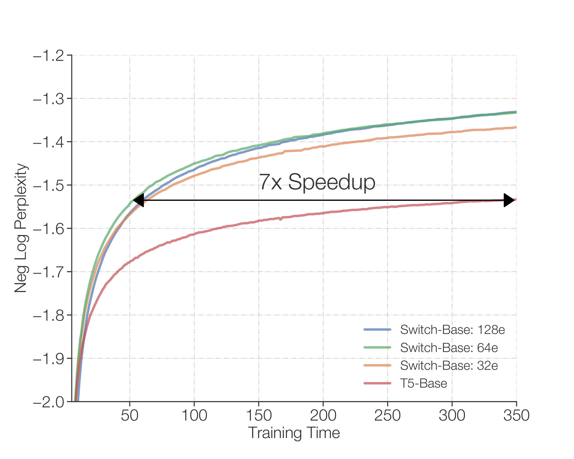
Switch models matched compute budgets of T5 baselines but held 30 times more parameters. Pre-training sped up 7 times versus T5-Base; trillion-parameter versions ran 4 times faster than T5-XXL. Negative log perplexity improved consistently with more experts. Downstream tasks gained: 4 points on SuperGLUE, 3 points on Winogrande over T5-Base. Multilingual pre-training improved all 101 languages, averaging 5 times faster steps. Distillation compressed models 99 percent while retaining 30 percent of gains.
4) Interpretation
These sparse models deliver more parameters without extra compute, cutting training time and costs. They boost performance on reasoning, knowledge, and multilingual tasks, shortening development timelines. Safety and compliance benefit from distillation, enabling smaller deployable models with near gains. No added risks noted, as sparsity leverages existing hardware.
5) Comparison to baselines/expectations
Switch outperformed dense T5 models and prior mixture-of-experts setups. It beat T5-Base despite same compute and topped T5-Large despite 3.5 times less compute per token. Single-expert routing simplified prior top-2 methods, yielding better speed and quality. Results exceeded expectations for stability and multilingual gains, matching scaling laws but along a new parameter axis.
6) Recommendations and next steps
Adopt Switch Transformers for new large language model training to gain speed and scale. Use 128 experts for base sizes, more for giants; distill outputs for production. Main option: pure expert parallelism for simplicity, or blend with model parallelism for higher compute—former suits memory limits, latter adds communication overhead. Test on target tasks before full rollout; run pilots with 2-8 experts on smaller hardware.
7) Limitations and confidence
Instability hit largest models sporadically, needing more fixes. Upstream gains sometimes translated unevenly to fine-tuning, especially reasoning tasks. Data focused on English-heavy corpora. High confidence in pre-training speedups and multilingual results (direct benchmarks); medium confidence in trillion-scale downstream due to partial training. Proceed with caution on ultra-large fine-tuning without extra validation.
In deep learning, models typically reuse the same parameters for all inputs. Mixture of Experts (MoE) models defy this and instead select different parameters for each incoming example. The result is a sparsely-activated model—with an outrageous number of parameters—but a constant computational cost. However, despite several notable successes of MoE, widespread adoption has been hindered by complexity, communication costs, and training instability. We address these with the introduction of the Switch Transformer. We simplify the MoE routing algorithm and design intuitive improved models with reduced communication and computational costs. Our proposed training techniques mitigate the instabilities, and we show large sparse models may be trained, for the first time, with lower precision (bfloat16) formats. We design models based off T5-Base and T5-Large ([1]) to obtain up to 7x increases in pre-training speed with the same computational resources. These improvements extend into multilingual settings where we measure gains over the mT5-Base version across all 101 languages. Finally, we advance the current scale of language models by pre-training up to trillion parameter models on the "Colossal Clean Crawled Corpus", and achieve a 4x speedup over the T5-XXL model.12
In this section, dense Transformer models excel at scale but incur prohibitive computational costs, driving the proposal of the sparsely-activated Switch Transformer, which simplifies Mixture-of-Experts routing to select unique parameters per input while fixing FLOPs. Overcoming MoE hurdles like complexity, communication, and instability via streamlined single-expert routing, selective bfloat16 precision, better initialization, and expert regularization, it yields 7x pre-training speedups over T5-Base/Large, universal multilingual gains across 101 languages, effective distillation retaining 30% quality improvements, and trillion-parameter models achieving 4x speedup versus T5-XXL.
Large scale training has been an effective path towards flexible and powerful neural language models ([2, 3, 4]). Simple architectures—backed by a generous computational budget, data set size and parameter count—surpass more complicated algorithms ([5]). An approach followed in [2, 1, 4] expands the model size of a densely-activated Transformer ([6]). While effective, it is also extremely computationally intensive ([7]). Inspired by the success of model scale, but seeking greater computational efficiency, we instead propose a sparsely-activated expert model: the Switch Transformer. In our case the sparsity comes from activating a subset of the neural network weights for each incoming example.
Sparse training is an active area of research and engineering ([8, 9]), but as of today, machine learning libraries and hardware accelerators still cater to dense matrix multiplications. To have an efficient sparse algorithm, we start with the Mixture-of-Expert (MoE) paradigm ([10, 11, 12]), and simplify it to yield training stability and computational benefits. MoE models have had notable successes in machine translation ([12, 13, 14]), however, widespread adoption is hindered by complexity, communication costs, and training instabilities.
We address these issues, and then go beyond translation, to find that these class of algorithms are broadly valuable in natural language. We measure superior scaling on a diverse set of natural language tasks and across three regimes in NLP: pre-training, fine-tuning and multi-task training. While this work focuses on scale, we also show that the Switch Transformer architecture not only excels in the domain of supercomputers, but is beneficial even with only a few computational cores. Further, our large sparse models can be distilled ([15]) into small dense versions while preserving 30% of the sparse model quality gain. Our contributions are the following:
The Switch Transformer architecture, which simplifies and improves over Mixture of Experts.
Scaling properties and a benchmark against the strongly tuned T5 model ([1]) where we measure 7x+ pre-training speedups while still using the same FLOPS per token. We further show the improvements hold even with limited computational resources, using as few as two experts.
Successful distillation of sparse pre-trained and specialized fine-tuned models into small dense models. We reduce the model size by up to 99% while preserving 30% of the quality gains of the large sparse teacher.
Improved pre-training and fine-tuning techniques: (1) selective precision training that enables training with lower bfloat16 precision (2) an initialization scheme that allows for scaling to a larger number of experts and (3) increased expert regularization that improves sparse model fine-tuning and multi-task training.
A measurement of the pre-training benefits on multilingual data where we find a universal improvement across all 101 languages and with 91% of languages benefiting from 4x+ speedups over the mT5 baseline ([16]).
An increase in the scale of neural language models achieved by efficiently combining data, model, and expert-parallelism to create models with up to a trillion parameters. These models improve the pre-training speed of a strongly tuned T5-XXL baseline by 4x.
2. Switch Transformer
Show me a brief summary.
In this section, scaling Transformer parameters massively while maintaining constant FLOPs per token drives the introduction of the Switch Transformer, a sparsely-activated model that replaces dense feed-forward layers with a simplified Mixture-of-Experts using single-expert (k=1) routing per token to minimize computation, batch sizes, and communication costs. Efficient distributed implementation via Mesh-Tensorflow incorporates fixed expert capacities scaled by a capacity factor to handle routing imbalances, augmented by a differentiable load-balancing loss that promotes uniform token dispatch. Training refinements—selective float32 precision for routers, 0.1x initialization scales, and expert dropout during fine-tuning—ensure stability across scales. Benchmarks confirm Switch Transformers surpass dense T5 and top-k MoE models in speed-quality, achieving top negative log perplexity fastest with capacity factors as low as 1.0.
The guiding design principle for Switch Transformers is to maximize the parameter count of a Transformer model ([6]) in a simple and computationally efficient way. The benefit of scale was exhaustively studied in [3] which uncovered power-law scaling with model size, data set size and computational budget.
Importantly, this work advocates training large models on relatively small amounts of data as the computationally optimal approach.
Heeding these results, we investigate a fourth axis: increase the parameter count while keeping the floating point operations (FLOPs) per example constant. Our hypothesis is that the parameter count, independent of total computation performed, is a separately important axis on which to scale. We achieve this by designing a sparsely activated model that efficiently uses hardware designed for dense matrix multiplications such as GPUs and TPUs. Our work here focuses on TPU architectures, but these class of models may be similarly trained on GPU clusters. In our distributed training setup, our sparsely activated layers split unique weights on different devices. Therefore, the weights of the model increase with the number of devices, all while maintaining a manageable memory and computational footprint on each device.
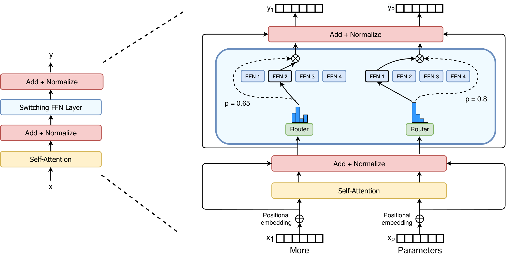
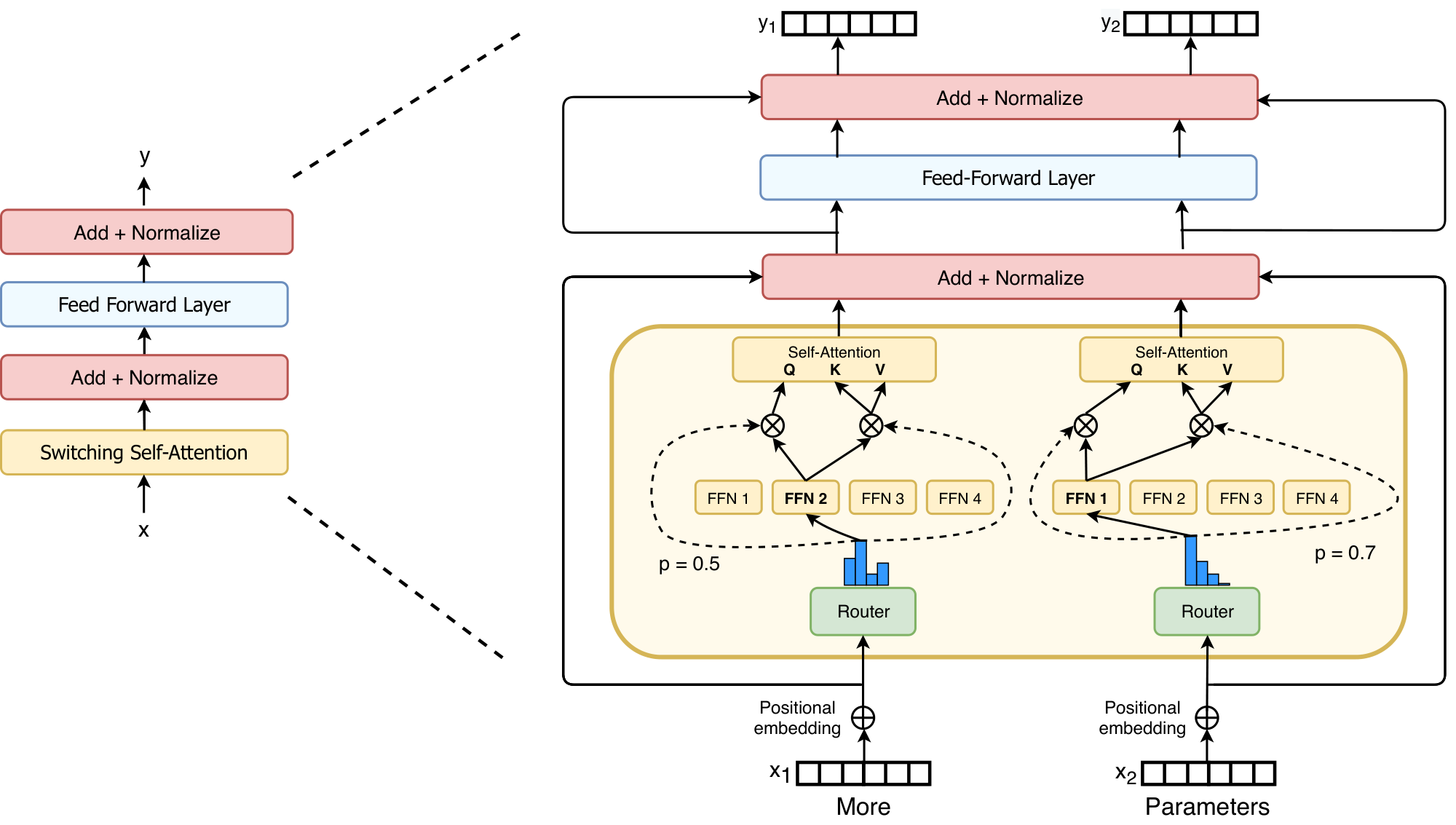
Figure 2: Illustration of a Switch Transformer encoder block. We replace the dense feed forward network (FFN) layer present in the Transformer with a sparse Switch FFN layer (light blue). The layer operates independently on the tokens in the sequence. We diagram two tokens (x1=“More" and x2=“Parameters" below) being routed (solid lines) across four FFN experts, where the router independently routes each token. The switch FFN layer returns the output of the selected FFN multiplied by the router gate value (dotted-line).
💭 Click to ask about this figure
2.1 Simplifying Sparse Routing
Mixture of Expert Routing. [12] proposed a natural language Mixture-of-Experts (MoE) layer which takes as an input a token representation xxx and then routes this to the best determined top- kkk experts, selected from a set {Ei(x)}i=1N\{E_i(x)\}_{i=1}^N{Ei(x)}i=1N of NNN experts. The router variable WrW_rWr produces logits h(x)=Wr⋅xh(x) = W_r \cdot xh(x)=Wr⋅x which are normalized via a softmax distribution over the available NNN experts at that layer. The gate-value for expert iii is given by,
pi(x)=∑jNeh(x)jeh(x)i.
💭 Click to ask about this equation
The top- kkk gate values are selected for routing the token xxx. If T\mathcal{T}T is the set of selected top- kkk indices then the output computation of the layer is the linearly weighted combination of each expert's computation on the token by the gate value,
y=i∈T∑pi(x)Ei(x).
💭 Click to ask about this equation
(1)
Switch Routing: Rethinking Mixture-of-Experts. [12] conjectured that routing to k>1k>1k>1 experts was necessary in order to have non-trivial gradients to the routing functions. The authors intuited that learning to route would not work without the ability to compare at least two experts. [17] went further to study the top- kkk decision and found that higher kkk-values in lower layers in the model were important for models with many routing layers. Contrary to these ideas, we instead use a simplified strategy where we route to only a single expert. We show this simplification preserves model quality, reduces routing computation and performs better. This k=1k=1k=1 routing strategy is later referred to as a Switch layer. Note that for both MoE and Switch Routing, the gate value pi(x)p_i(x)pi(x) in Equation 2 permits differentiability of the router.
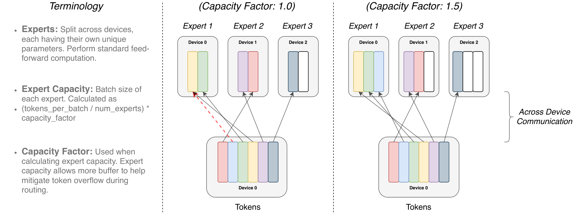
The benefits for the Switch layer are three-fold: (1) The router computation is reduced as we are only routing a token to a single expert. (2) The batch size (expert capacity) of each expert can be at least halved since each token is only being routed to a single expert.3(3) The routing implementation is simplified and communication costs are reduced. Figure 3 shows an example of routing with different expert capacity factors.
See Section 2.2 for a technical description.
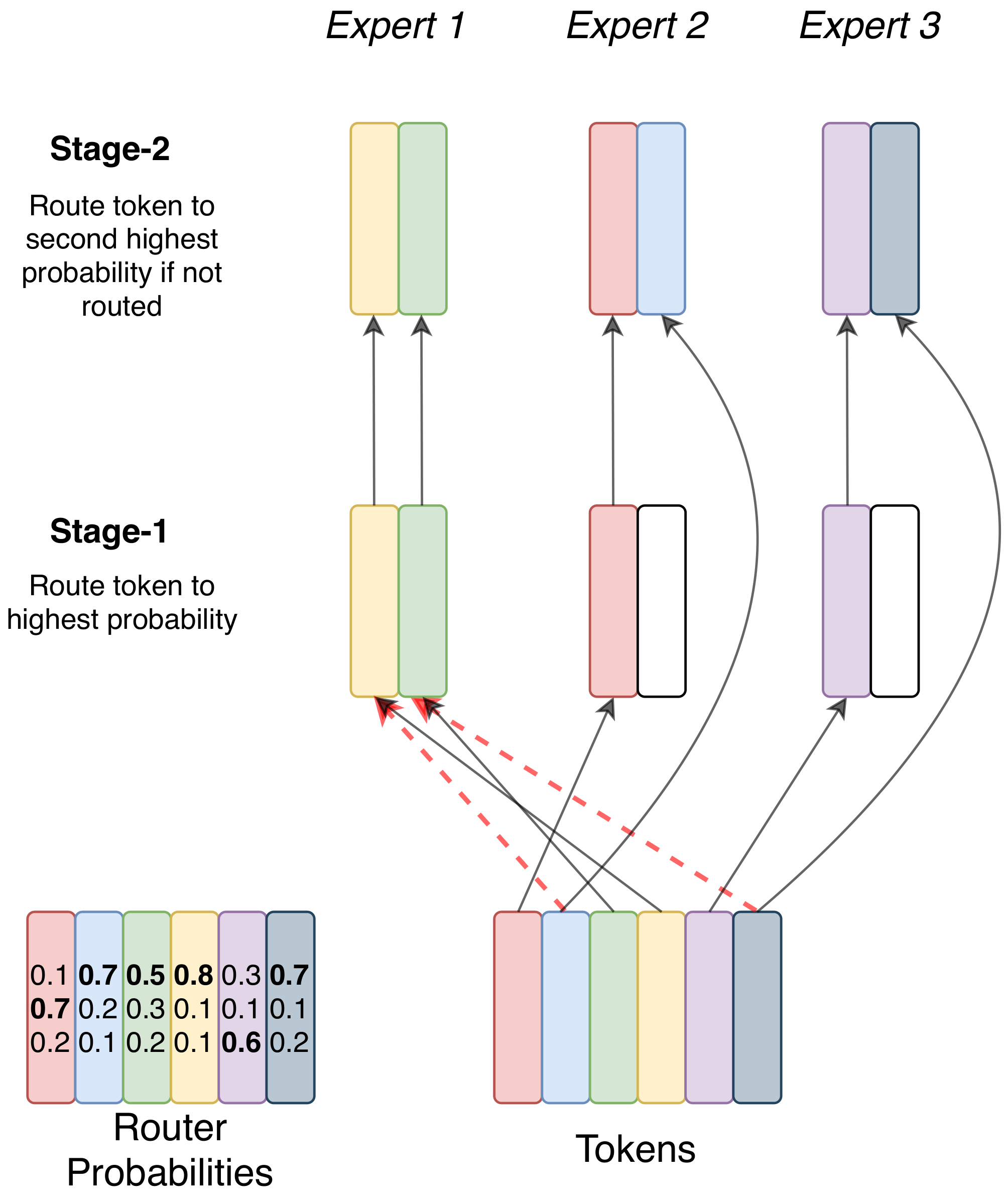
Figure 3: Illustration of token routing dynamics. Each expert processes a fixed batch-size of tokens modulated by the capacity factor. Each token is routed to the expert with the highest router probability, but each expert has a fixed batch size of (total_tokens / num_experts) × capacity_factor. If the tokens are unevenly dispatched then certain experts will overflow (denoted by dotted red lines), resulting in these tokens not being processed by this layer. A larger capacity factor alleviates this overflow issue, but also increases computation and communication costs (depicted by padded white/empty slots).
💭 Click to ask about this figure
2.2 Efficient Sparse Routing
We use Mesh-Tensorflow (MTF) ([13]) which is a library, with similar semantics and API to Tensorflow ([18]) that facilitates efficient distributed data and model parallel architectures. It does so by abstracting the physical set of cores to a logical mesh of processors. Tensors and computations may then be sharded per named dimensions, facilitating easy partitioning of models across dimensions. We design our model with TPUs in mind, which require statically declared sizes. Below we describe our distributed Switch Transformer implementation.
Distributed Switch Implementation. All of our tensor shapes are statically determined at compilation time, but our computation is dynamic due to the routing decisions at training and inference. Because of this, one important technical consideration is how to set the expert capacity. The expert capacity—the number of tokens each expert computes—is set by evenly dividing the number of tokens in the batch across the number of experts, and then further expanding by a capacity factor,
A capacity factor greater than 1.0 creates additional buffer to accommodate for when tokens are not perfectly balanced across experts. If too many tokens are routed to an expert (referred to later as dropped tokens), computation is skipped and the token representation is passed directly to the next layer through the residual connection. Increasing the expert capacity is not without drawbacks, however, since high values will result in wasted computation and memory. This trade-off is explained in Figure 3. Empirically we find ensuring lower rates of dropped tokens are important for the scaling of sparse expert-models. Throughout our experiments we didn't notice any dependency on the number of experts for the number of tokens dropped (typically <1%<1\%<1%). Using the auxiliary load balancing loss (next section) with a high enough coefficient ensured good load balancing. We study the impact that these design decisions have on model quality and speed in Table 1.
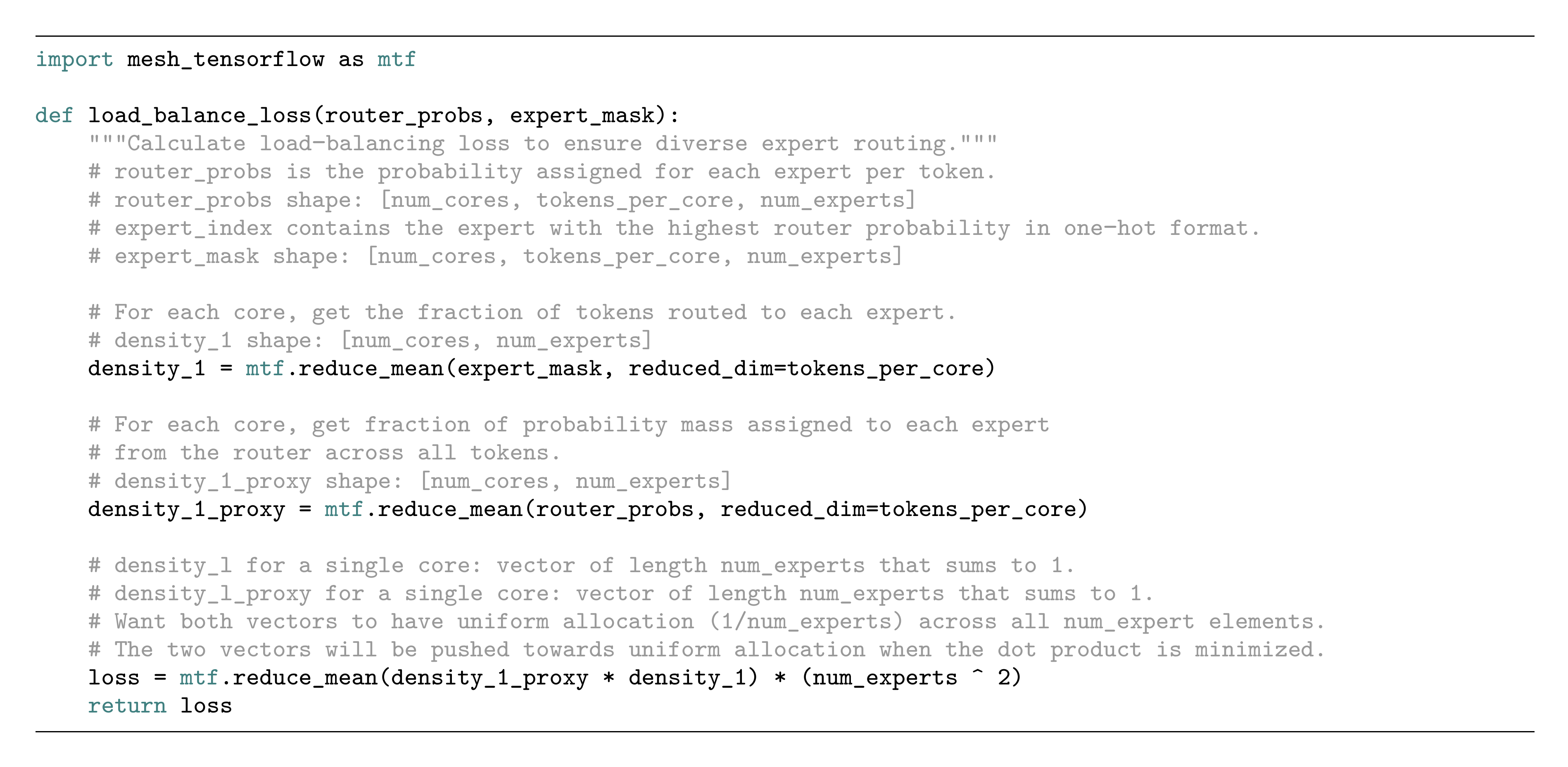
A Differentiable Load Balancing Loss. To encourage a balanced load across experts we add an auxiliary loss ([12, 13, 14]).
As in [13, 14], Switch Transformers simplifies the original design in [12] which had separate load-balancing and importance-weighting losses.
For each Switch layer, this auxiliary loss is added to the total model loss during training. Given NNN experts indexed by i=1i=1i=1 to NNN and a batch B\mathcal{B}B with TTT tokens, the auxiliary loss is computed as the scaled dot-product between vectors fff and PPP,
loss=α⋅N⋅i=1∑Nfi⋅Pi
💭 Click to ask about this equation
(2)
where fif_ifi is the fraction of tokens dispatched to expert iii,
fi=T1x∈B∑1{argmaxp(x)=i}
💭 Click to ask about this equation
(3)
and PiP_iPi is the fraction of the router probability allocated for expert iii, 4
A potential source of confusion: pi(x) is the probability of routing token x to expert i. Pi is the probability fraction to expert i across all tokens in the batch B.
Pi=T1x∈B∑pi(x).
💭 Click to ask about this equation
(4)
Since we seek uniform routing of the batch of tokens across the NNN experts, we desire both vectors to have values of 1/N1/N1/N. The auxiliary loss of Equation 2 encourages uniform routing since it is minimized under a uniform distribution. The objective can also be differentiated as the PPP-vector is differentiable, but the fff-vector is not. The final loss is multiplied by expert count NNN to keep the loss constant as the number of experts varies since under uniform routing ∑i=1N(fi⋅Pi)=∑i=1N(1N⋅1N)=1N\sum_{i=1}^N (f_i\cdot P_i) = \sum_{i=1}^N (\frac{1}{N}\cdot \frac{1}{N}) = \frac{1}{N}∑i=1N(fi⋅Pi)=∑i=1N(N1⋅N1)=N1. Finally, a hyper-parameter α\alphaα is a multiplicative coefficient for these auxiliary losses; throughout this work we use an α=10−2\alpha=10^{-2}α=10−2 which was sufficiently large to ensure load balancing while small enough to not to overwhelm the primary cross-entropy objective. We swept hyper-parameter ranges of α\alphaα from 10−110^{-1}10−1 to 10−510^{-5}10−5 in powers of 10 and found 10−210^{-2}10−2 balanced load quickly without interfering with training loss.
2.3 Putting It All Together: The Switch Transformer
Our first test of the Switch Transformer starts with pre-training on the ``Colossal Clean Crawled Corpus" (C4), introduced in ([1]). For our pre-training objective, we use a masked language modeling task ([19, 20, 21]) where the model is trained to predict missing tokens. In our pre-training setting, as determined in [1] to be optimal, we drop out 15% of tokens and then replace the masked sequence with a single sentinel token. To compare our models, we record the negative log perplexity.5 Throughout all tables in the paper, ↑\uparrow↑ indicates that a higher value for that metric is better and vice-versa for ↓\downarrow↓. A comparison of all the models studied in this work are in Table 9.
We use log base- e for this metric so the units are nats.
Table 1: Benchmarking Switch versus MoE. Head-to-head comparison measuring per step and per time benefits of the Switch Transformer over the MoE Transformer and T5 dense baselines. We measure quality by the negative log perplexity and the time to reach an arbitrary chosen quality threshold of Neg. Log Perp.=-1.50. All MoE and Switch Transformer models use 128 experts, with experts at every other feed-forward layer. For Switch-Base+, we increase the model size until it matches the speed of the MoE model by increasing the model hidden-size from 768 to 896 and the number of heads from 14 to 16. All models are trained with the same amount of computation (32 cores) and on the same hardware (TPUv3). Further note that all our models required pre-training beyond 100k steps to achieve our level threshold of -1.50. † T5-Base did not achieve this negative log perplexity in the 100k steps the models were trained.
Model
Capacity
Quality after
Time to Quality
Speed (↑)
Factor
100k steps (↑)
Threshold (↓)
(examples/sec)
(Neg. Log Perp.)
(hours)
T5-Base
—
-1.731
Not achieved†
1600
A head-to-head comparison of the Switch Transformer and the MoE Transformer is presented in Table 1. Our Switch Transformer model is FLOP-matched to 'T5-Base' ([1]) (same amount of computation per token is applied). The MoE Transformer, using top-2 routing, has two experts which each apply a separate FFN to each token and thus its FLOPS are larger. All models were trained for the same number of steps on identical hardware. Note that the MoE model going from capacity factor 2.0 to 1.25 actually slows down (840 to 790) in the above experiment setup, which is unexpected.6
Note that speed measurements are both a function of the algorithm and the implementation details. Switch Transformer reduces the necessary computation relative to MoE (algorithm), but the final speed differences are impacted by low-level optimizations (implementation).
We highlight three key findings from Table 1: (1) Switch Transformers outperform both carefully tuned dense models and MoE Transformers on a speed-quality basis. For a fixed amount of computation and wall-clock time, Switch Transformers achieve the best result. (2) The Switch Transformer has a smaller computational footprint than the MoE counterpart. If we increase its size to match the training speed of the MoE Transformer, we find this outperforms all MoE and Dense models on a per step basis as well. (3) Switch Transformers perform better at lower capacity factors (1.0, 1.25). Smaller expert capacities are indicative of the scenario in the large model regime where model memory is very scarce and the capacity factor will want to be made as small as possible.
2.4 Improved Training and Fine-Tuning Techniques
Sparse expert models may introduce training difficulties over a vanilla Transformer. Instability can result because of the hard-switching (routing) decisions at each of these layers. Further, low precision formats like bfloat16 ([22]) can exacerbate issues in the softmax computation for our router. We describe training difficulties here and the methods we use to overcome them to achieve stable and scalable training.
Selective precision with large sparse models. Model instability hinders the ability to train using efficient bfloat16 precision, and as a result, [14] trains with float32 precision throughout their MoE Transformer. However, we show that by instead selectively casting to float32 precision within a localized part of the model, stability may be achieved, without incurring expensive communication cost of float32 tensors. This technique is inline with modern mixed precision training strategies where certain parts of the model and gradient updates are done in higher precision [23]. Table 2 shows that our approach permits nearly equal speed to bfloat16 training while conferring the training stability of float32.
Table 2: Selective precision. We cast the local routing operations to float32 while preserving bfloat16 precision elsewhere to stabilize our model while achieving nearly equal speed to (unstable) bfloat16-precision training. We measure the quality of a 32 expert model after a fixed step count early in training its speed performance. For both Switch-Base in float32 and with Selective prevision we notice similar learning dynamics.
Model
Quality
Speed
(precision)
(Neg. Log Perp.) (↑)
(Examples/sec) (↑)
Switch-Base (float32)
-1.718
1160
Switch-Base (bfloat16)
-3.780 [diverged]
1390
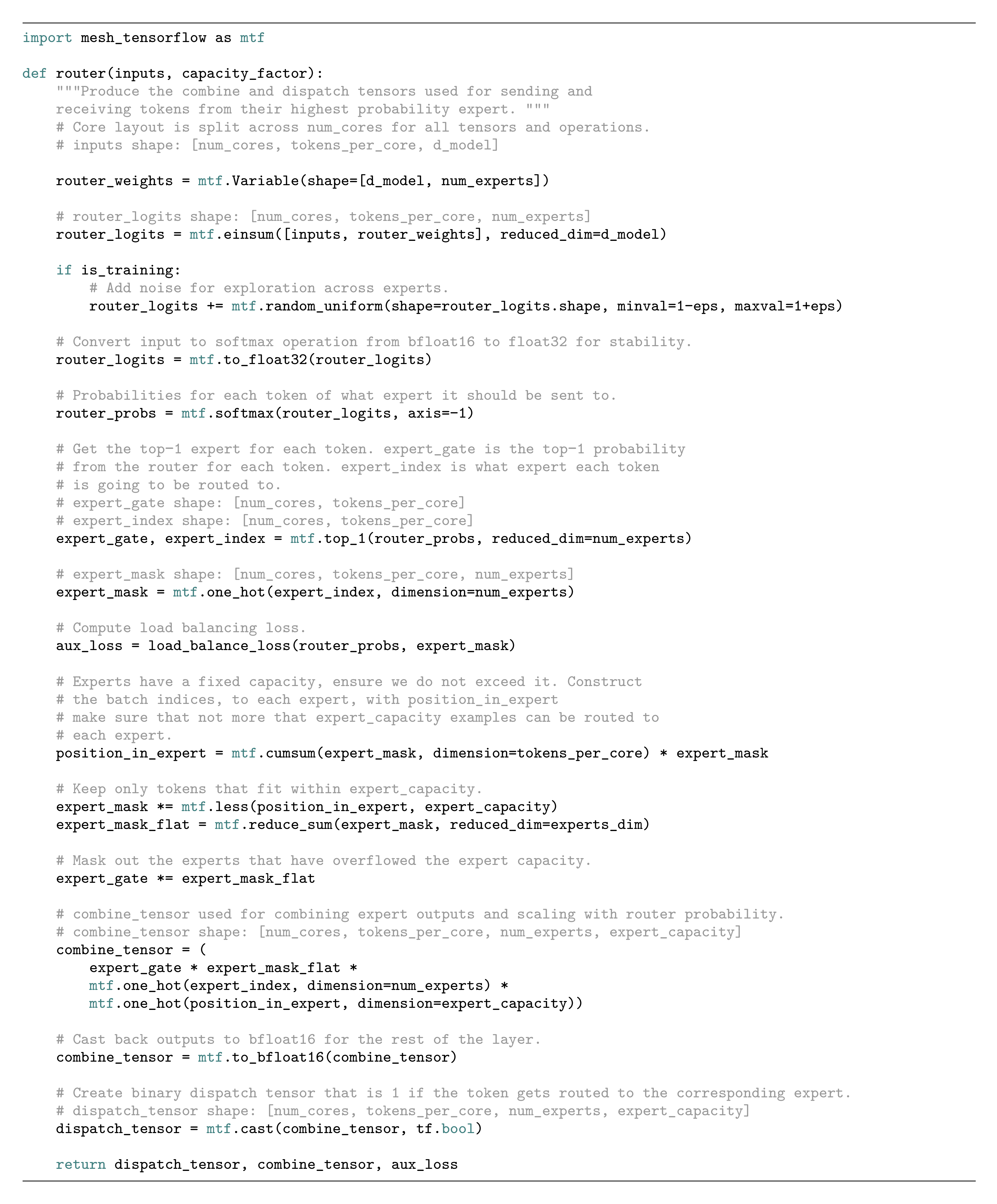
To achieve this, we cast the router input to float32 precision. The router function takes the tokens as input and produces the dispatch and combine tensors used for the selection and recombination of expert computation (refer to Code Block Figure 15 in the Appendix for details). Importantly, the float32 precision is only used within the body of the router function—on computations local to that device. Because the resulting dispatch and combine tensors are recast to bfloat16 precision at the end of the function, no expensive float32 tensors are broadcast through all-to-all communication operations, but we still benefit from the increased stability of float32.
Smaller parameter initialization for stability. Appropriate initialization is critical to successful training in deep learning and we especially observe this to be true for Switch Transformer. We initialize our weight matrices by drawing elements from a truncated normal distribution with mean μ=0\mu=0μ=0 and standard deviation σ=s/n\sigma=\sqrt{s / n}σ=s/n where sss is a scale hyper-parameter and nnn is the number of input units in the weight tensor (e.g. fan-in).7
Values greater than two standard deviations from the mean are resampled.
As an additional remedy to the instability, we recommend reducing the default Transformer initialization scale s=1.0s=1.0s=1.0 by a factor of 10. This both improves quality and reduces the likelihood of destabilized training in our experiments. Table 3 measures the improvement of the model quality and reduction of the variance early in training.
Table 3: Reduced initialization scale improves stability. Reducing the initialization scale results in better model quality and more stable training of Switch Transformer. Here we record the average and standard deviation of model quality, measured by the negative log perplexity, of a 32 expert model after 3.5k steps (3 random seeds each).
Model (Initialization scale)
Average Quality
Std. Dev. of Quality
(Neg. Log Perp.)
(Neg. Log Perp.)
Switch-Base (0.1x-init)
-2.72
0.01
Switch-Base (1.0x-init)
-3.60
0.68
We find that the average model quality, as measured by the Neg. Log Perp., is dramatically improved and there is a far reduced variance across runs. Further, this same initialization scheme is broadly effective for models spanning several orders of magnitude. We use the same approach to stably train models as small as our 223M parameter baseline to enormous models in excess of one trillion parameters.
Regularizing large sparse models. Our paper considers the common NLP approach of pre-training on a large corpus followed by fine-tuning on smaller downstream tasks such as summarization or question answering. One issue that naturally arises is overfitting since many fine-tuning tasks have very few examples. During fine-tuning of standard Transformers, [1] use dropout ([24]) at each layer to prevent overfitting. Our Switch Transformers have significantly more parameters than the FLOP matched dense baseline, which can lead to more severe overfitting on these smaller downstream tasks.
Table 4: Fine-tuning regularization results. A sweep of dropout rates while fine-tuning Switch Transformer models pre-trained on 34B tokens of the C4 data set (higher numbers are better). We observe that using a lower standard dropout rate at all non-expert layer, with a much larger dropout rate on the expert feed-forward layers, to perform the best.
Model (dropout)
GLUE
CNNDM
SQuAD
SuperGLUE
T5-Base (d=0.1)
82.9
19.6
83.5
72.4
Switch-Base (d=0.1)
84.7
19.1
83.7
73.0
Switch-Base (d=0.2)
84.4
19.2
83.9
73.2
We thus propose a simple way to alleviate this issue during fine-tuning: increase the dropout inside the experts, which we name as expert dropout. During fine-tuning we simply increase the dropout rate by a significant amount only at the interim feed-forward computation at each expert layer. Table 4 has the results for our expert dropout protocol. We observe that simply increasing the dropout across all layers leads to worse performance. However, setting a smaller dropout rate (0.1) at non-expert layers and a much larger dropout rate (0.4) at expert layers leads to performance improvements on four smaller downstream tasks.
3. Scaling Properties
Show me a brief summary.
In this section, the scaling properties of Switch Transformers are explored in pre-training on a vast corpus unbound by compute or data limits, focusing on experts as the prime scaling dimension to boost parameters without inflating token computation. With fixed FLOPs per token, more experts yield steady perplexity gains and superior sample efficiency per step, outpacing dense models. On wall-clock time with equal compute budgets, Switch-Base variants deliver massive speedups—64 experts match T5-Base quality in one-seventh the time—while even surpassing T5-Large's 3.5x higher FLOPs with 2.5x faster training, affirming sparse scaling's edge and potential for larger FLOP-matched designs like Switch-Large.
Show me a brief summary.
In this section, the appendix explores extensions and refinements to Switch Transformers, tackling challenges like routing stability, expert overflow, and scalability across regimes. It experiments with embedding Switch layers in self-attention for QKV projections, yielding quality gains but bfloat16 instability; proposes iterative rerouting to prevent token dropping, though without empirical benefits; favors input jitter over other exploration strategies for router decisions; demonstrates superiority even with just 2-8 experts at small scales; and correlates upstream perplexity with downstream SuperGLUE and TriviaQA performance, revealing strong scaling for Switch models on knowledge tasks but gaps in reasoning ones at large scales, alongside pseudocode for implementation. Ultimately, these validate sparse models' robustness while pinpointing stability and fine-tuning as key future hurdles.
We present a study of the scaling properties of the Switch Transformer architecture during pre-training. Per [3], we consider a regime where the model is not bottlenecked by either the computational budget or amount of data. To avoid the data bottleneck, we use the large C4 corpus with over 180B target tokens ([1]) and we train until diminishing returns are observed.
The number of experts is the most efficient dimension for scaling our model. Increasing the experts keeps the computational cost approximately fixed since the model only selects one expert per token, regardless of the number of experts to choose from. The router must compute a probability distribution over more experts, however, this is a lightweight computation of cost O(dmodel×num experts)O(d_{model} \times \text{num experts})O(dmodel×num experts) where dmodeld_{model}dmodel is the embedding dimension of tokens passed between the layers. In this section, we consider the scaling properties on a step-basis and a time-basis with a fixed computational budget.
3.1 Scaling Results on a Step-Basis
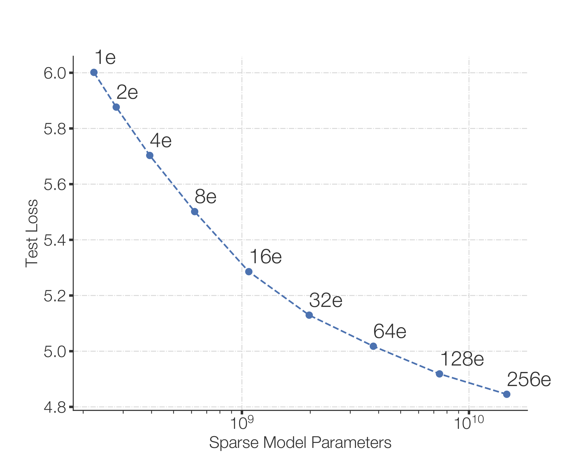
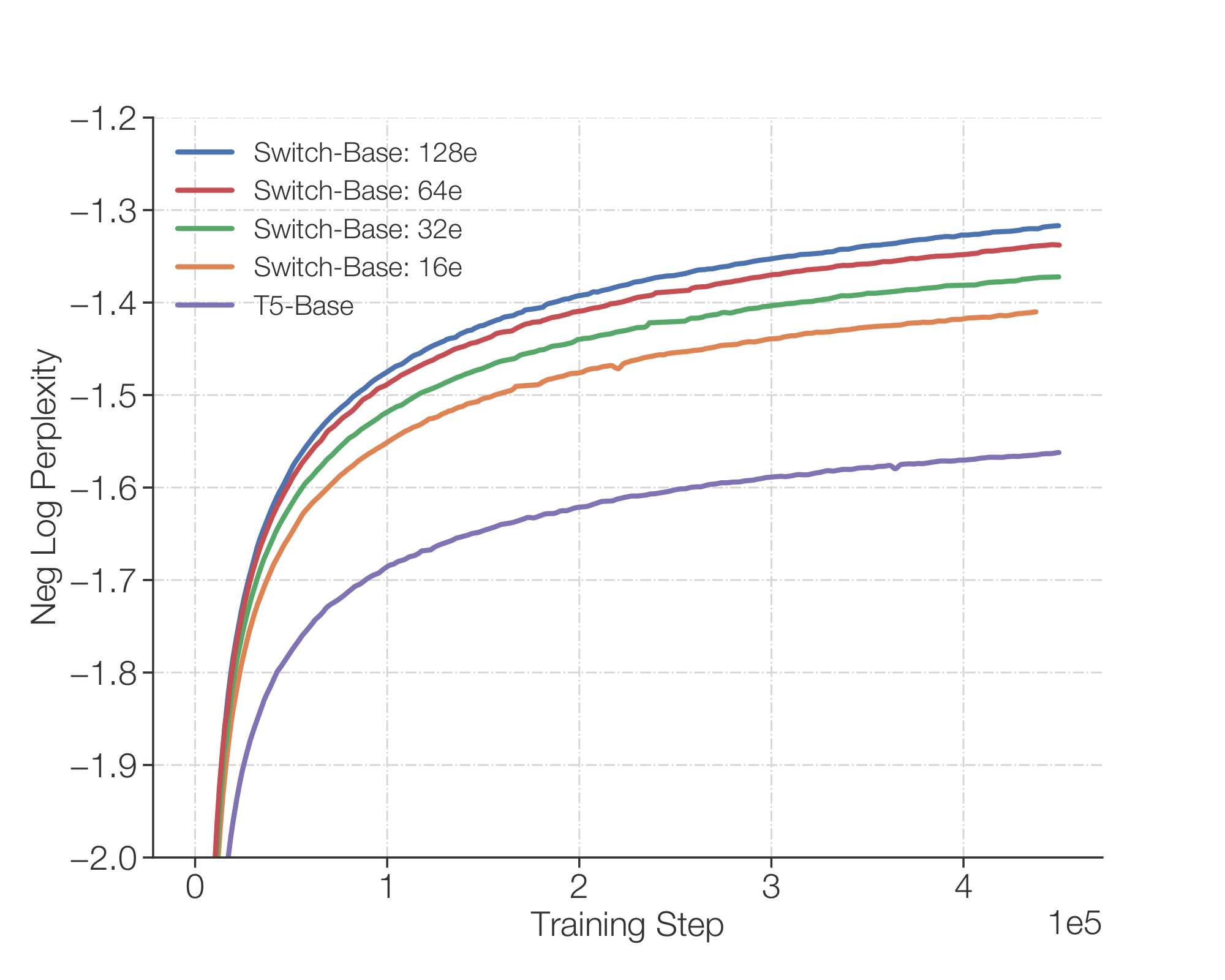
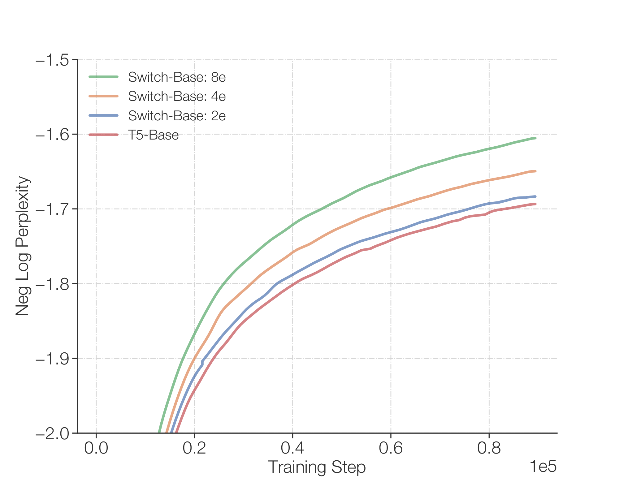
Figure 4 demonstrates consistent scaling benefits with the number of experts when training all models for a fixed number of steps. We observe a clear trend: when keeping the FLOPS per token fixed, having more parameters (experts) speeds up training. The left Figure demonstrates consistent scaling properties (with fixed FLOPS per token) between sparse model parameters and test loss. This reveals the advantage of scaling along this additional axis of sparse model parameters. Our right Figure measures sample efficiency of a dense model variant and four FLOP-matched sparse variants. We find that increasing the number of experts leads to more sample efficient models. Our Switch-Base 64 expert model achieves the same performance of the T5-Base model at step 60k at step 450k, which is a 7.5x speedup in terms of step time. In addition, consistent with the findings of [3], we find that larger models are also more sample efficient—learning more quickly for a fixed number of observed tokens.
Figure 4: Scaling properties of the Switch Transformer. Left Plot: We measure the quality improvement, as measured by perplexity, as the parameters increase by scaling the number of experts. The top-left point corresponds to the T5-Base model with 223M parameters. Moving from top-left to bottom-right, we double the number of experts from 2, 4, 8 and so on until the bottom-right point of a 256 expert model with 14.7B parameters. Despite all models using an equal computational budget, we observe consistent improvements scaling the number of experts. Right Plot: Negative log perplexity per step sweeping over the number of experts. The dense baseline is shown with the purple line and we note improved sample efficiency of our Switch-Base models.
💭 Click to ask about this figure
3.2 Scaling Results on a Time-Basis
Figure 4 demonstrates that on a step basis, as we increase the number of experts, the performance consistently improves. While our models have roughly the same amount of FLOPS per token as the baseline, our Switch Transformers incurs additional communication costs across devices as well as the extra computation of the routing mechanism. Therefore, the increased sample efficiency observed on a step-basis doesn't necessarily translate to a better model quality as measured by wall-clock. This raises the question:
For a fixed training duration and computational budget, should one train a dense or a sparse model?
Figure 5: Speed advantage of Switch Transformer. All models trained on 32 TPUv3 cores with equal FLOPs per example. For a fixed amount of computation and training time, Switch Transformers significantly outperform the dense Transformer baseline. Our 64 expert Switch-Base model achieves the same quality in one-seventh the time of the T5-Base and continues to improve.
💭 Click to ask about this figure
Figure 5 and Figure 6 address this question. Figure 5 measures the pre-training model quality as a function of time. For a fixed training duration and computational budget, Switch Transformers yield a substantial speed-up. In this setting, our Switch-Base 64 expert model trains in one-seventh the time that it would take the T5-Base to get similar perplexity.
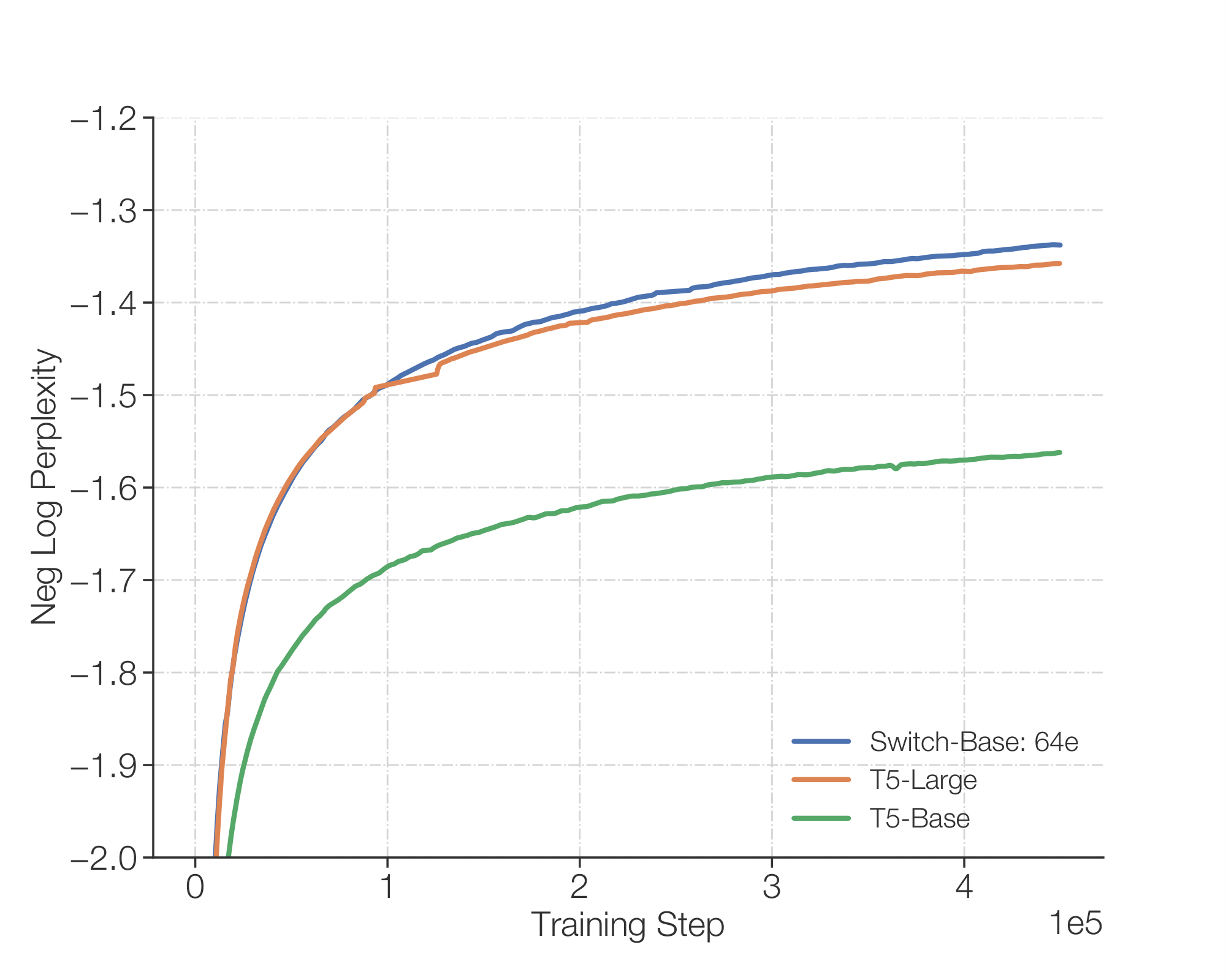
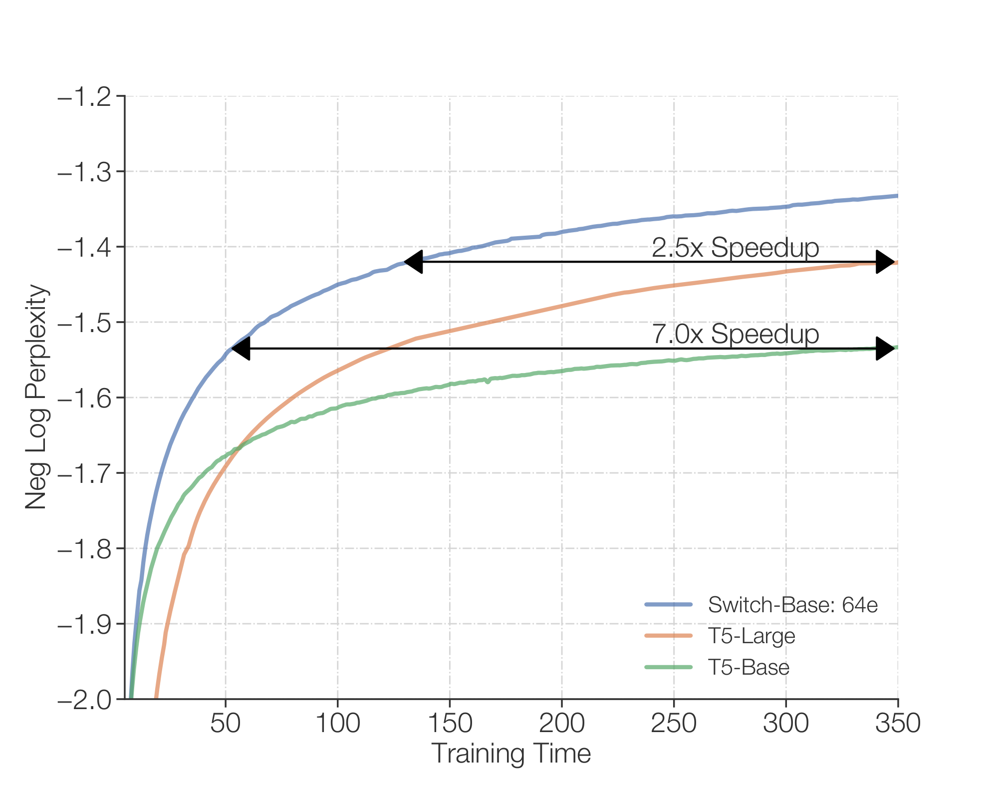
3.3 Scaling Versus a Larger Dense Model
The above analysis shows that a computationally-matched dense model is outpaced by its Switch counterpart. Figure 6 considers a different scenario: what if we instead had allocated our resources to a larger dense model? We do so now, measuring Switch-Base against the next strong baseline, T5-Large. But despite T5-Large applying 3.5x more FLOPs per token, Switch-Base is still more sample efficient and yields a 2.5x speedup. Furthermore, more gains can be had simply by designing a new, larger sparse version, Switch-Large, which is FLOP-matched to T5-Large. We do this and demonstrate superior scaling and fine-tuning in the following section.
Figure 6: Scaling Transformer models with Switch layers or with standard dense model scaling. Left Plot: Switch-Base is more sample efficient than both the T5-Base, and T5-Large variant, which applies 3.5x more FLOPS per token. Right Plot: As before, on a wall-clock basis, we find that Switch-Base is still faster, and yields a 2.5x speedup over T5-Large.
💭 Click to ask about this figure
4. Downstream Results
Show me a brief summary.
In this section, the key question is whether Switch Transformers' pre-training advantages persist in downstream NLP applications. Fine-tuning FLOP-matched Switch models outperforms T5 baselines across diverse tasks like GLUE, SuperGLUE, SQuAD, Winogrande, summarization, and closed-book QA, yielding gains in reasoning and knowledge-intensive benchmarks. Distillation shrinks billion-parameter sparse teachers by 95%+ into 223M dense students, retaining 30% of quality improvements via expert-weight initialization and mixed losses. Multilingual pre-training on 101 languages boosts perplexity universally for mSwitch-Base over mT5-Base, with a mean 5x step speedup and 91% of languages at 4x or greater. Overall, Switch Transformers confirm scalable, deployable superiority in multi-task and multilingual settings.
Section 3 demonstrated the superior scaling properties while pre-training, but we now validate that these gains translate to improved language learning abilities on downstream tasks. We begin by fine-tuning on a diverse set of NLP tasks. Next we study reducing the memory footprint of our sparse models by over 90% by distilling into small—and easily deployed—dense baselines. Finally, we conclude this section measuring the improvements in a multi-task, multilingual setting, where we show that Switch Transformers are strong multi-task learners, improving over the multilingual T5-base model across all 101 languages.
4.1 Fine-Tuning
Baseline and Switch models used for fine-tuning. Our baselines are the highly-tuned 223M parameter T5-Base model and the 739M parameter T5-Large model ([1]). For both versions, we design a FLOP-matched Switch Transformer, with many more parameters, which is summarized in Table 9.8
FLOPS are calculated for the forward pass as done in [3].
Our baselines differ slightly from those in [1] because we pre-train on an improved C4 corpus which removes intra-example text duplication and thus increases the efficacy as a pre-training task [25]. In our protocol we pre-train with 2202^{20}220 (1, 048, 576) tokens per batch for 550k steps amounting to 576B total tokens. We then fine-tune across a diverse set of tasks using a dropout rate of 0.1 for all layers except the Switch layers, which use a dropout rate of 0.4 (see Table 4). We fine-tune using a batch-size of 1M for 16k steps and for each task, we evaluate model quality every 200-steps and report the peak performance as computed on the validation set.
Fine-tuning tasks and data sets. We select tasks probing language capabilities including question answering, summarization and knowledge about the world. The language benchmarks GLUE ([26]) and SuperGLUE ([27]) are handled as composite mixtures with all the tasks blended in proportion to the amount of tokens present in each. These benchmarks consist of tasks requiring sentiment analysis (SST-2), word sense disambiguation (WIC), sentence similarty (MRPC, STS-B, QQP), natural language inference (MNLI, QNLI, RTE, CB), question answering (MultiRC, RECORD, BoolQ), coreference resolution (WNLI, WSC) and sentence completion (COPA) and sentence acceptability (CoLA). The CNNDM ([28]) and BBC XSum ([29]) data sets are used to measure the ability to summarize articles. Question answering is probed with the SQuAD data set ([30]) and the ARC Reasoning Challenge ([31]). And as in [32], we evaluate the knowledge of our models by fine-tuning on three closed-book question answering data sets: Natural Questions ([33]), Web Questions ([34]) and Trivia QA ([35]). Closed-book refers to questions posed with no supplemental reference or context material. To gauge the model's common sense reasoning we evaluate it on the Winogrande Schema Challenge ([36]). And finally, we test our model's natural language inference capabilities on the Adversarial NLI Benchmark ([37]).
Table 5: Fine-tuning results. Fine-tuning results of T5 baselines and Switch models across a diverse set of natural language tests (validation sets; higher numbers are better). We compare FLOP-matched Switch models to the T5-Base and T5-Large baselines. For most tasks considered, we find significant improvements of the Switch-variants. We observe gains across both model sizes and across both reasoning and knowledge-heavy language tasks.
GLUE
SQuAD
SuperGLUE
Winogrande (XL)
T5-Base
84.3
85.5
75.1
66.6
Switch-Base
86.7
87.2
79.5
73.3
T5-Large
87.8
88.1
82.7
79.1
Switch-Large
88.5
88.6
84.7
83.0
Fine-tuning metrics. The following evaluation metrics are used throughout the paper: We report the average scores across all subtasks for GLUE and SuperGLUE. The Rouge-2 metric is used both the CNNDM and XSum. In SQuAD and the closed book tasks (Web, Natural, and Trivia Questions) we report the percentage of answers exactly matching the target (refer to [32] for further details and deficiency of this measure). Finally, in ARC Easy, ARC Challenge, ANLI, and Winogrande we report the accuracy of the generated responses.
Fine-tuning results. We observe significant downstream improvements across many natural language tasks. Notable improvements come from SuperGLUE, where we find FLOP-matched Switch variants improve by 4.4 and 2 percentage points over the T5-Base and T5-Large baselines, respectively as well as large improvements in Winogrande, closed book Trivia QA, and XSum.9 In our fine-tuning study, the only tasks where we do not observe gains are on the AI2 Reasoning Challenge (ARC) data sets where the T5-Base outperforms Switch-Base on the challenge data set and T5-Large outperforms Switch-Large on the easy data set. Taken as a whole, we observe significant improvements spanning both reasoning and knowledge-heavy tasks. This validates our architecture, not just as one that pre-trains well, but can translate quality improvements to downstream tasks via fine-tuning.
Our T5 and Switch models were pre-trained with 220 tokens per batch for 550k steps on a revised C4 data set for fair comparisons.
4.2 Distillation
Deploying massive neural networks with billions, or trillions, of parameters is inconvenient. To alleviate this, we study distilling ([15]) large sparse models into small dense models. Future work could additionally study distilling large models into smaller sparse models.
Distillation techniques. In Table 6 we study a variety of distillation techniques. These techniques are built off of [38], who study distillation methods for BERT models. We find that initializing the dense model with the non-expert weights yields a modest improvement. This is possible since all models are FLOP matched, so non-expert layers will have the same dimensions. Since expert layers are usually only added at every or every other FFN layer in a Transformer, this allows for many of the weights to be initialized with trained parameters. Furthermore, we observe a distillation improvement using a mixture of 0.25 for the teacher probabilities and 0.75 for the ground truth label. By combining both techniques we preserve ≈\approx≈ 30% of the quality gains from the larger sparse models with only ≈1/20th\approx1/20^{th}≈1/20th of the parameters. The quality gain refers to the percent of the quality difference between Switch-Base (Teacher) and T5-Base (Student). Therefore, a quality gain of 100% implies the Student equals the performance of the Teacher.
Table 6: Distilling Switch Transformers for Language Modeling. Initializing T5-Base with the non-expert weights from Switch-Base and using a loss from a mixture of teacher and ground-truth labels obtains the best performance. We can distill 30% of the performance improvement of a large sparse model with 100x more parameters back into a small dense model. For a final baseline, we find no improvement of T5-Base initialized with the expert weights, but trained normally without distillation.
Technique
Parameters
Quality (↑)
T5-Base
223M
-1.636
Switch-Base
3, 800M
-1.444
Distillation
223M
(3%) -1.631
Achievable compression rates. Using our best distillation technique described in Table 6, we distill a wide variety of sparse models into dense models. We distill Switch-Base versions, sweeping over an increasing number of experts, which corresponds to varying between 1.1B to 14.7B parameters. Through distillation, we can preserve 37% of the quality gain of the 1.1B parameter model while compressing 82%. At the extreme, where we compress the model 99%, we are still able to maintain 28% of the teacher's model quality improvement.
Table 7: Distillation compression rates. We measure the quality when distilling large sparse models into a dense baseline. Our baseline, T5-Base, has a -1.636 Neg. Log Perp. quality. In the right columns, we then distill increasingly large sparse models into this same architecture. Through a combination of weight-initialization and a mixture of hard and soft losses, we can shrink our sparse teachers by 95%+ while preserving 30% of the quality gain. However, for significantly better and larger pre-trained teachers, we expect larger student models would be necessary to achieve these compression rates.
Dense
Sparse
Parameters
223M
1.1B
2.0B
3.8B
7.4B
14.7B
Pre-trained Neg. Log Perp. (↑)
-1.636
-1.505
-1.474
-1.444
-1.432
-1.427
Distilled Neg. Log Perp. (↑)
—
-1.587
-1.585
-1.579
-1.582
-1.578
Percent of Teacher Performance
—
37%
32%
30 %
27 %
28 %
Compression Percent
—
82 %
90 %
95 %
97 %
99 %
Distilling a fine-tuned model. We conclude this with a study of distilling a fine-tuned sparse model into a dense model. Table 8 shows results of distilling a 7.4B parameter Switch-Base model, fine-tuned on the SuperGLUE task, into the 223M T5-Base. Similar to our pre-training results, we find we are able to preserve 30% of the gains of the sparse model when distilling into a FLOP matched dense variant. One potential future avenue, not considered here, may examine the specific experts being used for fine-tuning tasks and extracting them to achieve better model compression.
Table 8: Distilling a fine-tuned SuperGLUE model. We distill a Switch-Base model fine-tuned on the SuperGLUE tasks into a T5-Base model. We observe that on smaller data sets our large sparse model can be an effective teacher for distillation. We find that we again achieve 30% of the teacher's performance on a 97% compressed model.
Model
Parameters
FLOPS
SuperGLUE (↑)
T5-Base
223M
124B
74.6
Switch-Base
7410M
124B
81.3
Distilled T5-Base
223M
124B
(30%) 76.6
4.3 Multilingual Learning
In our final set of downstream experiments, we measure the model quality and speed tradeoffs while pre-training on a mixture of 101 different languages. We build and benchmark off the recent work of mT5 ([16]), a multilingual extension to T5. We pre-train on the multilingual variant of the Common Crawl data set (mC4) spanning 101 languages introduced in mT5, but due to script variants within certain languages, the mixture contains 107 tasks.
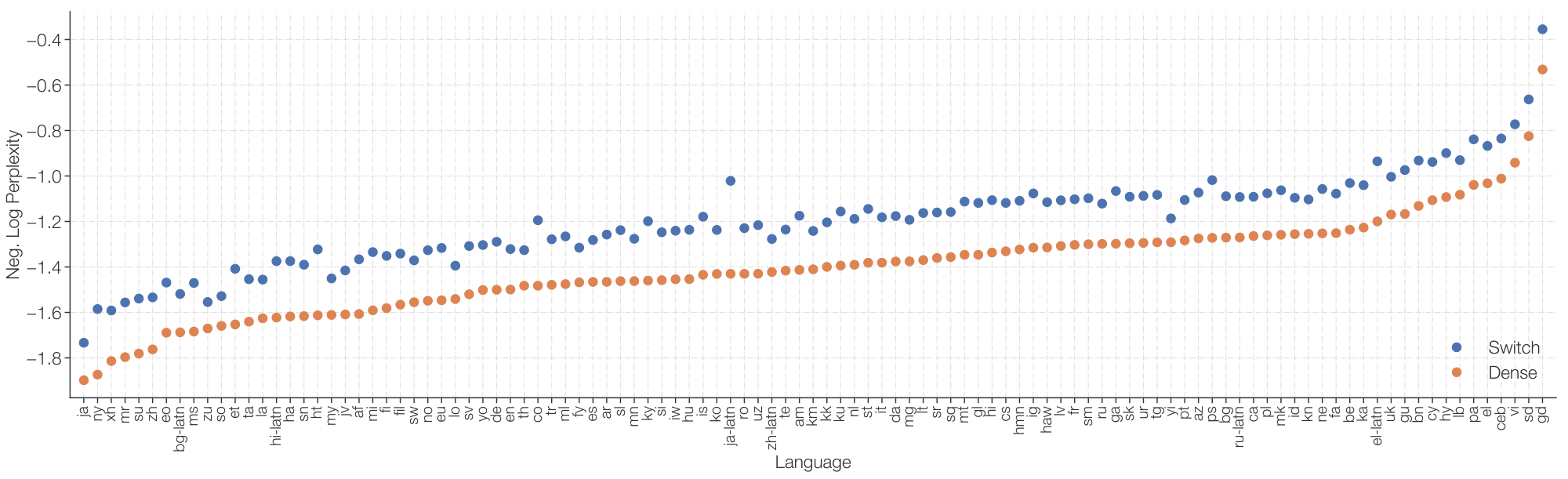
Figure 7: Multilingual pre-training on 101 languages. Improvements of Switch T5 Base model over dense baseline when multi-task training on 101 languages. We observe Switch Transformers to do quite well in the multi-task training setup and yield improvements on all 101 languages.
💭 Click to ask about this figure
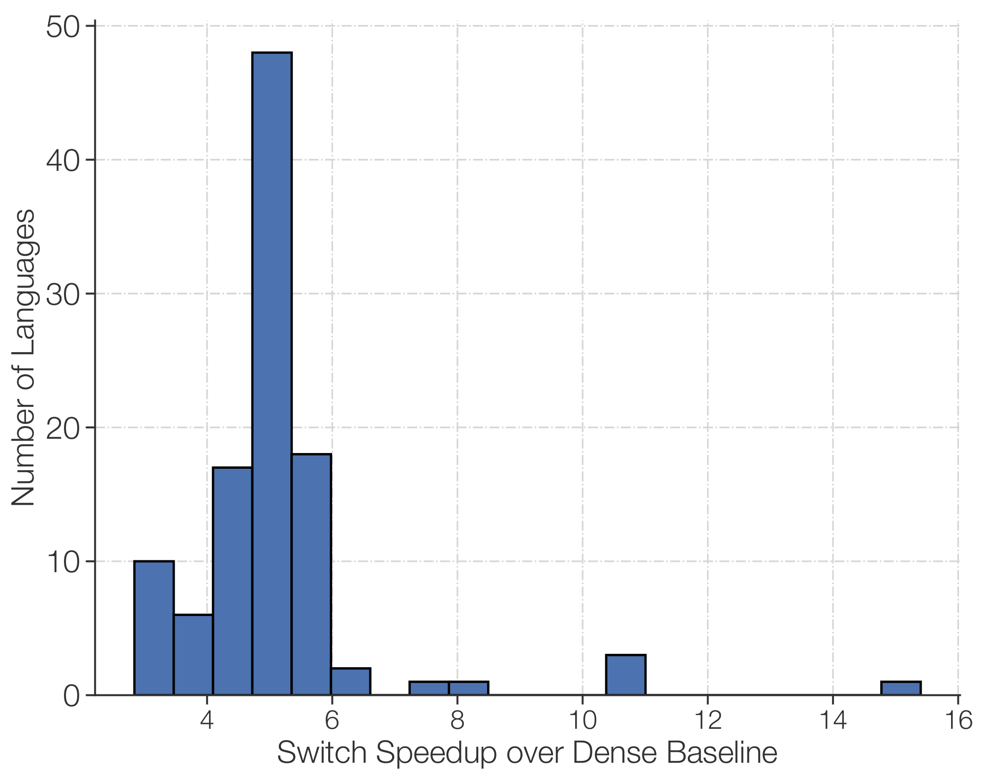
Figure 8: Multilingual pre-training on 101 languages. We histogram for each language, the step speedup of Switch Transformers over the FLOP matched T5 dense baseline to reach the same quality. Over all 101 languages, we achieve a mean step speed-up over mT5-Base of 5x and, for 91% of languages, we record a 4x, or greater, speedup to reach the final perplexity of mT5-Base.
💭 Click to ask about this figure
In Figure 7 we plot the quality improvement in negative log perplexity for all languages of a FLOP-matched Switch model, mSwitch-Base to the T5 base variant, mT5-Base. After pre-training both versions for 1M steps, we find that on all 101 languages considered, Switch Transformer increases the final negative log perplexity over the baseline. In Figure 8, we present a different view and now histogram the per step speed-up of using Switch Transformer over the mT5-Base.10 We find a mean speed-up over mT5-Base of 5x and that 91% of languages achieve at least a 4x speedup. This presents evidence that Switch Transformers are effective multi-task and multi-lingual learners.
The speedup on a step basis is computed as the ratio of the number of steps for the baseline divided by the number of steps required by our model to reach that same quality.
5. Designing Models with Data, Model, and Expert-Parallelism
Show me a brief summary.
In this section, scaling Switch Transformers beyond diminishing returns from more experts requires balancing parameters, FLOPs, and memory via data, model, and expert-parallelism on FFN layers. It reviews partitioning strategies—data-parallelism shards batches across cores with end-of-pass all-reduces; model-parallelism shards weights inducing per-layer communication; hybrids combine them, while expert-parallelism routes tokens via all-to-all to capacity-limited experts per core. Combining all three enables trillion-parameter models like FLOP-matched Switch-XXL (395B params) and expert-only Switch-C (1.6T params), which outperform T5-XXL in pre-training perplexity on C4 despite less data and instability in larger FLOPs setups, yielding comparable or state-of-the-art downstream results, especially on knowledge tasks.
Arbitrarily increasing the number of experts is subject to diminishing returns (Figure 4). Here we describe complementary scaling strategies. The common way to scale a Transformer is to increase dimensions in tandem, like dmodeld_{model}dmodel or dffd_{ff}dff. This increases both the parameters and computation performed and is ultimately limited by the memory per accelerator. Once it exceeds the size of the accelerator's memory, single program multiple data (SPMD) model-parallelism can be employed. This section studies the trade-offs of combining data, model, and expert-parallelism.
Reviewing the Feed-Forward Network (FFN) Layer. We use the FFN layer as an example of how data, model and expert-parallelism works in Mesh TensorFlow ([13]) and review it briefly here. We assume BBB tokens in the batch, each of dimension dmodeld_{model}dmodel. Both the input (xxx) and output (yyy) of the FFN are of size [BBB, dmodeld_{model}dmodel] and the intermediate (hhh) is of size [BBB, dffd_{ff}dff] where dffd_{ff}dff is typically several times larger than dmodeld_{model}dmodel. In the FFN, the intermediate is h=xWinh=x W_{in}h=xWin and then the output of the layer is y=ReLU(h)Wouty = ReLU(h) W_{out}y=ReLU(h)Wout. Thus WinW_{in}Win and WoutW_{out}Wout are applied independently to each token and have sizes [dmodeld_{model}dmodel, dffd_{ff}dff] and [dffd_{ff}dff, dmodeld_{model}dmodel].
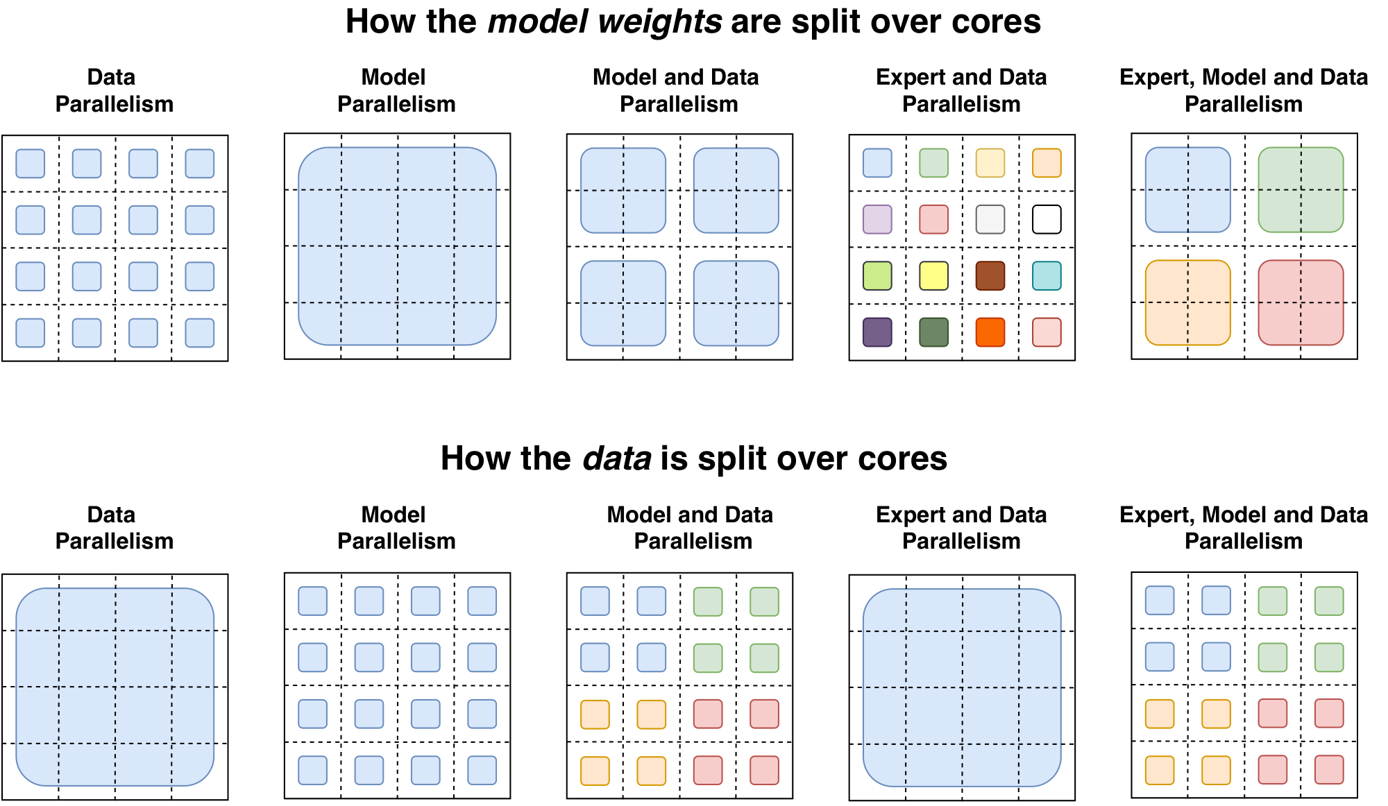
We describe two aspects of partitioning: how the weights and batches of data divide over cores, depicted in Figure 9. We denote all cores available as NNN which Mesh Tensorflow may then remap into a logical multidimensional mesh of processors. Here we create a two-dimensional logical mesh, with one dimension representing the number of ways for data-parallel sharding (nnn) and the other, the model-parallel sharding (mmm). The total cores must equal the ways to shard across both data and model-parallelism, e.g. N=n×mN = n \times mN=n×m. To shard the layer across cores, the tensors containing that batch of BBB tokens are sharded across nnn data-parallel cores, so each core contains B/nB / nB/n tokens. Tensors and variables with dffd_{ff}dff are then sharded across mmm model-parallel cores. For the variants with experts-layers, we consider EEE experts, each of which can process up to CCC tokens.
Term
Description
B
Number of tokens in the batch.
N
Number of total cores.
n
Number of ways for data-parallelism sharding.
m
Number of ways for model-parallelism sharding.
Figure 9: Data and weight partitioning strategies. Each 4 × 4 dotted-line grid represents 16 cores and the shaded squares are the data contained on that core (either model weights or batch of tokens). We illustrate both how the model weights and the data tensors are split for each strategy. First Row: illustration of how model weights are split across the cores. Shapes of different sizes in this row represent larger weight matrices in the Feed Forward Network (FFN) layers (e.g larger dff sizes). Each color of the shaded squares identifies a unique weight matrix. The number of parameters per core is fixed, but larger weight matrices will apply more computation to each token. Second Row: illustration of how the data batch is split across cores. Each core holds the same number of tokens which maintains a fixed memory usage across all strategies. The partitioning strategies have different properties of allowing each core to either have the same tokens or different tokens across cores, which is what the different colors symbolize.
💭 Click to ask about this figure
5.1 Data Parallelism
When training data parallel models, which is the standard for distributed training, then all cores are allocated to the data-parallel dimension or n=N,m=1n = N, m = 1n=N,m=1. This has the advantage that no communication is needed until the entire forward and backward pass is finished and the gradients need to be then aggregated across all cores. This corresponds to the left-most column of Figure 9.
5.2 Model Parallelism
We now consider a scenario where all cores are allocated exclusively to the model-parallel dimension and so n=1,m=Nn = 1, m = Nn=1,m=N. Now all cores must keep the full BBB tokens and each core will contain a unique slice of the weights. For each forward and backward pass, a communication cost is now incurred. Each core sends a tensor of [BBB, dmodeld_{model}dmodel] to compute the second matrix multiplication ReLU(h)WoutReLU(h) W_{out}ReLU(h)Wout because the dffd_{ff}dff dimension is partitioned and must be summed over. As a general rule, whenever a dimension that is partitioned across cores must be summed, then an all-reduce operation is added for both the forward and backward pass. This contrasts with pure data parallelism where an all-reduce only occurs at the end of the entire forward and backward pass.
5.3 Model and Data Parallelism
It is common to mix both model and data parallelism for large scale models, which was done in the largest T5 models ([1, 16]) and in GPT-3 ([4]). With a total of N=n×mN = n \times mN=n×m cores, now each core will be responsible for B/nB / nB/n tokens and dff/md_{ff} / mdff/m of both the weights and intermediate activation. In the forward and backward pass each core communicates a tensor of size [B/n,dmodel][B / n, d_{model}][B/n,dmodel] in an all-reduce operation.
5.4 Expert and Data Parallelism
Next we describe the partitioning strategy for expert and data parallelism. Switch Transformers will allocate all of their cores to the data partitioning dimension nnn, which will also correspond to the number of experts in the model. For each token per core a router locally computes assignments to the experts. The output is a binary matrix of size [nnn, B/nB / nB/n, EEE, CCC] which is partitioned across the first dimension and determines expert assignment. This binary matrix is then used to do a gather via matrix multiplication with the input tensor of [nnn, B/nB / nB/n, dmodeld_{model}dmodel].
resulting in the final tensor of shape [nnn, EEE, CCC, dmodeld_{model}dmodel], which is sharded across the first dimension. Because each core has its own expert, we do an all-to-all communication of size [EEE, CCC, dmodeld_{model}dmodel] to now shard the EEE dimension instead of the nnn-dimension. There are additional communication costs of bfloat16 tensors of size E×C×dmodelE \times C \times d_{model}E×C×dmodel in the forward pass to analogusly receive the tokens from each expert located on different cores. See Appendix F for a detailed analysis of the expert partitioning code.
5.5 Expert, Model and Data Parallelism
In the design of our best model, we seek to balance the FLOPS per token and the parameter count. When we scale the number of experts, we increase the number of parameters, but do not change the FLOPs per token. In order to increase FLOPs, we must also increase the dffd_{ff}dff dimension (which also increases parameters, but at a slower rate). This presents a trade-off: as we increase dffd_{ff}dff we will run out of memory per core, which then necessitates increasing mmm. But since we have a fixed number of cores NNN, and N=n×mN=n \times mN=n×m, we must decrease nnn, which forces use of a smaller batch-size (in order to hold tokens per core constant).
When combining both model and expert-parallelism, we will have all-to-all communication costs from routing the tokens to the correct experts along with the internal all-reduce communications from the model parallelism. Balancing the FLOPS, communication costs and memory per core becomes quite complex when combining all three methods where the best mapping is empirically determined. See our further analysis in Section 5.6 for how the number of experts effects the downstream performance as well.
5.6 Towards Trillion Parameter Models
Combining expert, model and data parallelism, we design two large Switch Transformer models, one with 395 billion and 1.6 trillion parameters, respectively. We study how these models perform on both up-stream pre-training as language models and their downstream fine-tuning performance. The parameters, FLOPs per sequence and hyper-parameters of the two different models are listed below in Table 9. Standard hyper-parameters of the Transformer, including dmodeld_{model}dmodel, dffd_{ff}dff, dkvd_{kv}dkv, number of heads and number of layers are described, as well as a less common feature, FFNGEGLUFFN_{GEGLU}FFNGEGLU, which refers to a variation of the FFN layer where the expansion matrix is substituted with two sets of weights which are non-linearly combined ([39]).
Table 9: Switch model design and pre-training performance. We compare the hyper-parameters and pre-training performance of the T5 models to our Switch Transformer variants. The last two columns record the pre-training model quality on the C4 data set after 250k and 500k steps, respectively. We observe that the Switch-C Transformer variant is 4x faster to a fixed perplexity (with the same compute budget) than the T5-XXL model, with the gap increasing as training progresses.
Parameters
FLOPs/seq
dmodel
FFNGEGLU
dff
dkv
Num. Heads
T5-Base
0.2B
124B
768
✓
2048
64
12
T5-Large
0.7B
425B
1024
✓
2816
64
16
T5-XXL
11B
6.3T
4096
✓
10240
64
64
Switch-Base
7B
124B
768
✓
2048
64
12
The Switch-C model is designed using only expert-parallelism, and no model-parallelism, as described earlier in Section 5.4. As a result, the hyper-parameters controlling the width, depth, number of heads, and so on, are all much smaller than the T5-XXL model. In contrast, the Switch-XXL is FLOP-matched to the T5-XXL model, which allows for larger dimensions of the hyper-parameters, but at the expense of additional communication costs induced by model-parallelism (see Section 5.5 for more details).
Sample efficiency versus T5-XXL. In the final two columns of Table 9 we record the negative log perplexity on the C4 corpus after 250k and 500k steps, respectively. After 250k steps, we find both Switch Transformer variants to improve over the T5-XXL version's negative log perplexity by over 0.061.11 To contextualize the significance of a gap of 0.061, we note that the T5-XXL model had to train for an additional 250k steps to increase 0.052. The gap continues to increase with additional training, with the Switch-XXL model out-performing the T5-XXL by 0.087 by 500k steps.
This reported quality difference is a lower bound, and may actually be larger. The T5-XXL was pre-trained on an easier C4 data set which included duplicated, and thus easily copied, snippets within examples.
Training instability. However, as described in the introduction, large sparse models can be unstable, and as we increase the scale, we encounter some sporadic issues. We find that the larger Switch-C model, with 1.6T parameters and 2048 experts, exhibits no training instability at all. Instead, the Switch XXL version, with nearly 10x larger FLOPs per sequence, is sometimes unstable. As a result, though this is our better model on a step-basis, we do not pre-train for a full 1M steps, in-line with the final reported results of T5 ([1]).
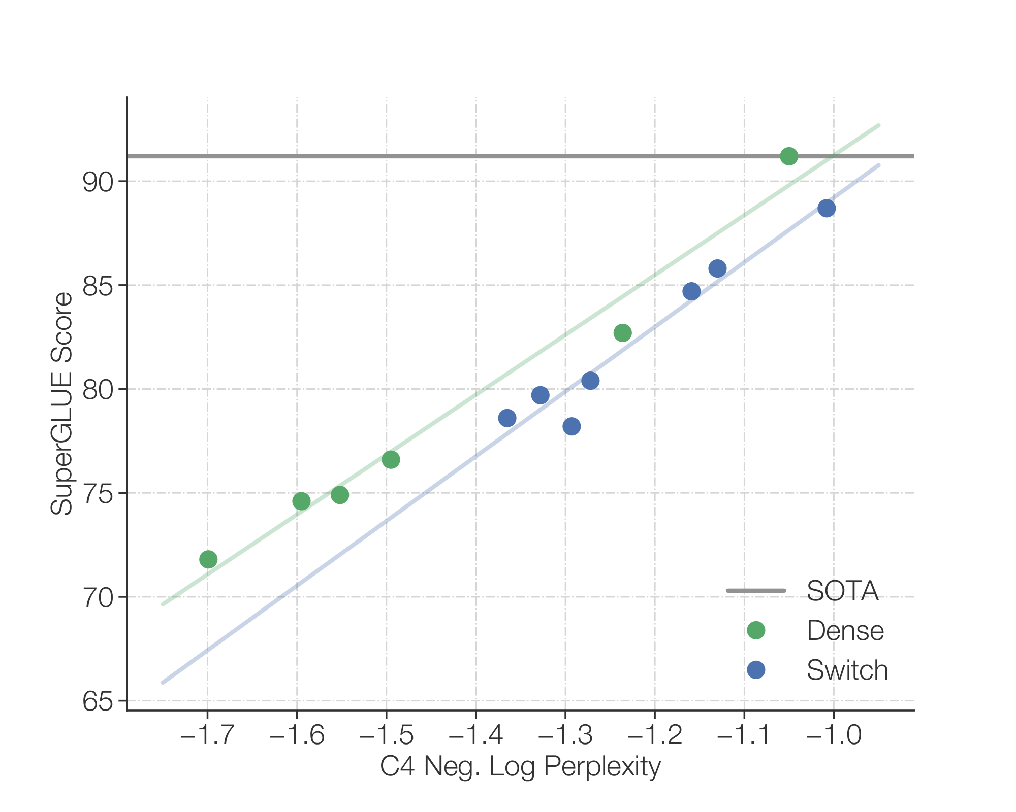
Reasoning fine-tuning performance. As a preliminary assessment of the model quality, we use a Switch-XXL model partially pre-trained on 503B tokens, or approximately half the text used by the T5-XXL model. Using this checkpoint, we conduct multi-task training for efficiency, where all tasks are learned jointly, rather than individually fine-tuned. We find that SQuAD accuracy on the validation set increases to 89.7 versus state-of-the-art of 91.3. Next, the average SuperGLUE test score is recorded at 87.5 versus the T5 version obtaining a score of 89.3 compared to the state-of-the-art of 90.0 ([27]). On ANLI ([37]), Switch XXL improves over the prior state-of-the-art to get a 65.7 accuracy versus the prior best of 49.4 ([40]). We note that while the Switch-XXL has state-of-the-art Neg. Log Perp. on the upstream pre-training task, its gains have not yet fully translated to SOTA downstream performance. We study this issue more in Appendix E.
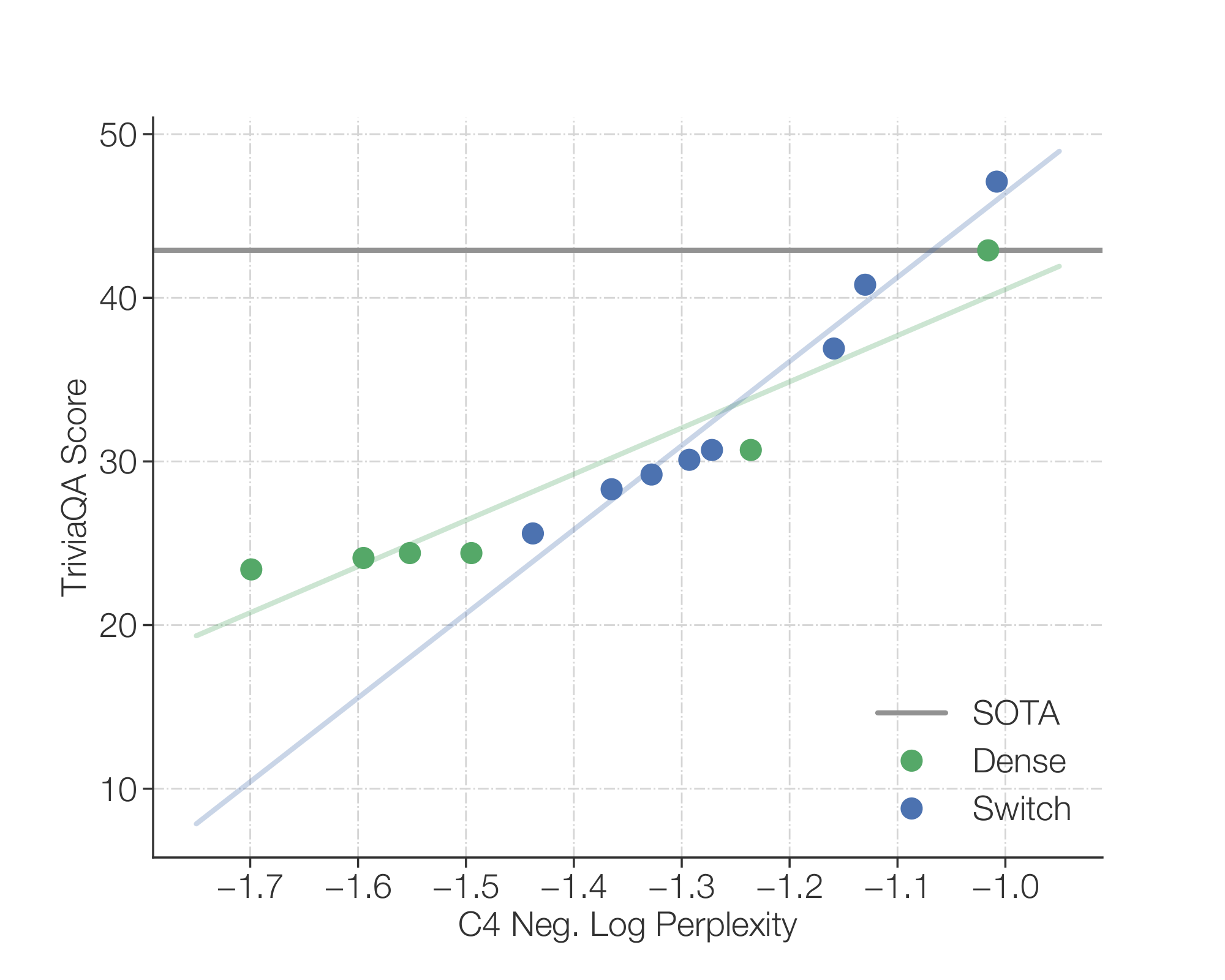
Knowledge-based fine-tuning performance. Finally, we also conduct an early examination of the model's knowledge with three closed-book knowledge-based tasks: Natural Questions, WebQuestions and TriviaQA, without additional pre-training using Salient Span Masking ([41]). In all three cases, we observe improvements over the prior state-of-the-art T5-XXL model (without SSM). Natural Questions exact match increases to 34.4 versus the prior best of 32.8, Web Questions increases to 41.0 over 37.2, and TriviaQA increases to 47.5 versus 42.9.
Summing up, despite training on less than half the data of other models, we already find comparable, and sometimes state-of-the-art, model quality. Currently, the Switch Transformer translates substantial upstream gains better to knowledge-based tasks, than reasoning-tasks (see Appendix E). Extracting stronger fine-tuning performance from large expert models is an active research question, and the pre-training perplexity indicates future improvements should be possible.
6. Related Work
Show me a brief summary.
In this section, scaling neural networks to billions of parameters drives innovations like model parallelism for weight sharding, pipeline parallelism for layer distribution, and product key lookups for capacity, alongside conditional computation that dynamically routes inputs to specialized experts. Mixture of Experts layers excelled between LSTMs for language tasks, reemerged in Transformers via Mesh Tensorflow without NLP benchmarks, and powered GShard's multilingual translation gains, with deterministic variants partitioning parameters by language. Attention sparsity along sequence length curbs quadratic complexity for longer contexts, positioning Switch Transformers as a complementary sparse architecture ripe for integration to enhance long-range learning.
The importance of scale in neural networks is widely recognized and several approaches have been proposed. Recent works have scaled models to billions of parameters through using model parallelism (e.g. splitting weights and tensors across multiple cores) ([13, 42, 1, 4, 43]). Alternatively, [44, 45] propose using pipeline based model parallelism, where different layers are split across devices and micro-batches are pipelined to the different layers. Finally, Product Key networks ([46]) were proposed to scale up the capacity of neural networks by doing a lookup for learnable embeddings based on the incoming token representations to a given layer.
Our work studies a specific model in a class of methods that do conditional computation, where computation decisions are made dynamically based on the input. [47] proposed adaptively selecting weights based on certain bit patterns occuring in the model hidden-states. [48] built stacked expert layers with dense matrix multiplications and ReLU activations and showed promising results on jittered MNIST and monotone speech. In computer vision [49] manually route tokens based on semantic classes during upstream pre-training and then select the relevant experts to be used according to the downstream task.
Mixture of Experts (MoE), in the context of modern deep learning architectures, was proven effective in [12]. That work added an MoE layer which was stacked between LSTM ([50]) layers, and tokens were separately routed to combinations of experts. This resulted in state-of-the-art results in language modeling and machine translation benchmarks. The MoE layer was reintroduced into the Transformer architecture by the Mesh Tensorflow library ([13]) where MoE layers were introduced as a substitute of the FFN layers, however, there were no accompanying NLP results. More recently, through advances in machine learning infrastructure, GShard ([14]), which extended the XLA compiler, used the MoE Transformer to dramatically improve machine translation across 100 languages. Finally [51] chooses a different deterministic MoE strategy to split the model parameters into non-overlapping groups of languages.
Sparsity along the sequence length dimension (LLL) in the Transformer attention patterns has been a successful technique to reduce the attention complexity from O(L2)O(L^2)O(L2) ([52, 53, 54, 55, 56, 57]). This has enabled learning longer sequences than previously possible. This version of the Switch Transformer does not employ attention sparsity, but these techniques are complimentary, and, as future work, these could be combined to potentially improve learning on tasks requiring long contexts.
7. Discussion
Show me a brief summary.
In this section, the discussion tackles skepticism around Switch Transformers by addressing why sparse expert models outperform dense counterparts despite challenges like deployment scale and hardware optimization. It affirms their edge through parameter scaling for better sample efficiency, viability on everyday GPUs with few experts, superiority on speed-accuracy curves per step and wall-clock time, distillability for smaller models retaining much quality, and time-based efficiency over sharded dense models—while allowing hybrid use. Historically hindered by dense models' dominance, complexity, instability, and communication overhead, sparse models like Switch Transformer now overcome these barriers, proving faster and more effective at equivalent compute.
We pose and discuss questions about the Switch Transformer, and sparse expert models generally, where sparsity refers to weights, not on attention patterns.
Isn't Switch Transformer better due to sheer parameter count? Yes, and by design! Parameters, independent of the total FLOPs used, are a useful axis to scale neural language models. Large models have been exhaustively shown to perform better ([3]). But in this case, our model is more sample efficient and faster while using the same computational resources.
I don't have access to a supercomputer—is this still useful for me? Though this work has focused on extremely large models, we also find that models with as few as two experts improves performance while easily fitting within memory constraints of commonly available GPUs or TPUs (details in Appendix D). We therefore believe our techniques are useful in small-scale settings.
Do sparse models outperform dense models on the speed-accuracy Pareto curve? Yes. Across a wide variety of different models sizes, sparse models outperform dense models per step and on wall clock time. Our controlled experiments show for a fixed amount of computation and time, sparse models outperform dense models.
I can't deploy a trillion parameter model—can we shrink these models? We cannot fully preserve the model quality, but compression rates of 10 to 100x are achievable by distilling our sparse models into dense models while achieving ≈\approx≈ 30% of the quality gain of the expert model.
Why use Switch Transformer instead of a model-parallel dense model? On a time basis, Switch Transformers can be far more efficient than dense-models with sharded parameters (Figure 6). Also, we point out that this decision is not mutually exclusive—we can, and do, use model-parallelism in Switch Transformers, increasing the FLOPs per token, but incurring the slowdown of conventional model-parallelism.
Why aren't sparse models widely used already? The motivation to try sparse models has been stymied by the massive success of scaling dense models (the success of which is partially driven by co-adaptation with deep learning hardware as argued in [58]). Further, sparse models have been subject to multiple issues including (1) model complexity, (2) training difficulties, and (3) communication costs. Switch Transformer makes strides to alleviate these issues.
8. Future Work
Show me a brief summary.
In this section, Switch Transformers face unresolved challenges in scaling sparse expert models, including training instability at massive sizes, unclear links between pre-training perplexity, FLOPs per token, and fine-tuning quality, and optimal blending of data, model, and expert parallelism. Key directions include enhancing stability via regularizers and clipping, deriving hardware-guided scaling laws, enabling heterogeneous experts for adaptive computation on hard examples, placing experts beyond FFN layers like in self-attention (with promising but unstable preliminary gains), and extending to new modalities. These pursuits promise to fully realize sparse models' efficiency and performance potential across diverse tasks and architectures.
This paper lays out a simplified architecture, improved training procedures, and a study of how sparse models scale. However, there remain many open future directions which we briefly describe here:
A significant challenge is further improving training stability for the largest models. While our stability techniques were effective for our Switch-Base, Switch-Large and Switch-C models (no observed instability), they were not sufficient for Switch-XXL. We have taken early steps towards stabilizing these models, which we think may be generally useful for large models, including using regularizers for improving stability and adapted forms of gradient clipping, but this remains unsolved.
Generally we find that improved pre-training quality leads to better downstream results (Appendix E), though we sometimes encounter striking anomalies. For instance, despite similar perplexities modeling the C4 data set, the 1.6T parameter Switch-C achieves only an 87.7 exact match score in SQuAD, which compares unfavorably to 89.6 for the smaller Switch-XXL model. One notable difference is that the Switch-XXL model applies ≈\approx≈ 10x the FLOPS per token than the Switch-C model, even though it has ≈\approx≈ 4x less unique parameters (395B vs 1.6T). This suggests a poorly understood dependence between fine-tuning quality, FLOPS per token and number of parameters.
Perform a comprehensive study of scaling relationships to guide the design of architectures blending data, model and expert-parallelism. Ideally, given the specs of a hardware configuration (computation, memory, communication) one could more rapidly design an optimal model. And, vice versa, this may also help in the design of future hardware.
Our work falls within the family of adaptive computation algorithms. Our approach always used identical, homogeneous experts, but future designs (facilitated by more flexible infrastructure) could support heterogeneous experts. This would enable more flexible adaptation by routing to larger experts when more computation is desired—perhaps for harder examples.
Investigating expert layers outside the FFN layer of the Transformer. We find preliminary evidence that this similarly can improve model quality. In Appendix A, we report quality improvement adding these inside Self-Attention layers, where our layer replaces the weight matrices which produce Q, K, V. However, due to training instabilities with the bfloat16 format, we instead leave this as an area for future work.
Examining Switch Transformer in new and across different modalities. We have thus far only considered language, but we believe that model sparsity can similarly provide advantages in new modalities, as well as multi-modal networks.
This list could easily be extended, but we hope this gives a flavor for the types of challenges that we are thinking about and what we suspect are promising future directions.
9. Conclusion
Show me a brief summary.
In this section, scaling neural language models to trillions of parameters demands efficiency and stability beyond dense architectures. Switch Transformers simplify Mixture of Experts into an intuitive, trainable design that vastly outperforms equivalently sized dense models in sample efficiency. They excel across pre-training, fine-tuning, and multi-task regimes on diverse NLP tasks, enabling hundred-billion to trillion-parameter training with major speedups over T5 baselines, thus positioning sparse models as a compelling paradigm for NLP and beyond.
Switch Transformers are scalable and effective natural language learners. We simplify Mixture of Experts to produce an architecture that is easy to understand, stable to train and vastly more sample efficient than equivalently-sized dense models. We find that these models excel across a diverse set of natural language tasks and in different training regimes, including pre-training, fine-tuning and multi-task training. These advances make it possible to train models with hundreds of billion to trillion parameters and which achieve substantial speedups relative to dense T5 baselines. We hope our work motivates sparse models as an effective architecture and that this encourages researchers and practitioners to consider these flexible models in natural language tasks, and beyond.
10. Acknowledgments
Show me a brief summary.
In this section, the authors credit a vital network of collaborators for enabling the Switch Transformer's breakthroughs in scalability and efficiency. Margaret Li delivered pivotal algorithmic insights and empirical guidance over months, Hugo Larochelle provided sage advice and draft refinements, Irwan Bello offered meticulous revisions, and Colin Raffel plus Adam Roberts supplied crucial T5 expertise. Yoshua Bengio inspired adaptive computation efforts, Jascha Sohl-Dickstein advanced large-model stabilization, the Google Brain Team fueled key discussions, and Blake Hechtman optimized training speed. This collective input transformed challenges into a stable, high-performing architecture.
The authors would like to thank Margaret Li who provided months of key insights into algorithmic improvements and suggestions for empirical studies. Hugo Larochelle for sage advising and clarifying comments on the draft, Irwan Bello for detailed comments and careful revisions, Colin Raffel and Adam Roberts for timely advice on neural language models and the T5 code-base, Yoshua Bengio for advising and encouragement on research in adaptive computation, Jascha Sohl-dickstein for interesting new directions for stabilizing new large scale models and paper revisions, and the Google Brain Team for useful discussions on the paper. Blake Hechtman who provided invaluable help in profiling and improving the training performance of our models.
Appendix
A. Switch for Attention
[13, 14] designed MoE Transformers ([12]) by adding MoE layers into the dense feedfoward network (FFN) computations of the Transformer. Similarly, our work also replaced the FFN layer in the Transformer, but we briefly explore here an alternate design. We add Switch layers into the Transformer Self-Attention layers. To do so, we replace the trainable weight matrices that produce the queries, keys and values with Switch layers as seen in Figure 10.
Figure 10: Switch layers in attention. We diagram how to incorporate the Switch layer into the Self-Attention transformer block. For each token (here we show two tokens, x1=“More" and x2=“Parameters"), one set of weights produces the query and the other set of unique weights produces the shared keys and values. We experimented with each expert being a linear operation, as well as a FFN, as was the case throughout this work. While we found quality improvements using this, we found this to be more unstable when used with low precision number formats, and thus leave it for future work.
💭 Click to ask about this figure
Table 10 records the quality after a fixed number of steps as well as training time for several variants. Though we find improvements, we also found these layers to be more unstable when using bfloat16 precision and thus we did not include them in the final variant. However, when these layers do train stably, we believe the preliminary positive results suggests a future promising direction.
Table 10: Switch attention layer results. All models have 32 experts and train with 524k tokens per batch. Experts FF is when experts replace the FFN in the Transformer, which is our standard setup throughout the paper. Experts FF + Attention is when experts are used to replace both the FFN and the Self-Attention layers. When training with bfloat16 precision the models that have experts attention diverge.
Model
Precision
Quality
Quality
Speed
@100k Steps (↑)
@16H (↑)
(ex/sec) (↑)
Experts FF
float32
-1.548
-1.614
1480
Expert Attention
float32
-1.524
-1.606
1330
B. Preventing Token Dropping with No-Token-Left-Behind
Due to software constraints on TPU accelerators, the shapes of our Tensors must be statically sized. As a result, each expert has a finite and fixed capacity to process token representations. This, however, presents an issue for our model which dynamically routes tokens at run-time that may result in an uneven distribution over experts. If the number of tokens sent to an expert is less than the expert capacity, then the computation may simply be padded – an inefficient use of the hardware, but mathematically correct. However, when the number of tokens sent to an expert is larger than its capacity (expert overflow), a protocol is needed to handle this. [14] adapts a Mixture-of-Expert model and addresses expert overflow by passing its representation to the next layer without processing through a residual connection which we also follow.
We suspected that having no computation applied to tokens could be very wasteful, especially since if there is overflow on one expert, that means another expert will have extra capacity. With this intuition we create No-Token-Left-Behind, which iteratively reroutes any tokens that are at first routed to an expert that is overflowing. Figure 11 shows a graphical description of this method, which will allow us to guarantee almost no tokens will be dropped during training and inference. We hypothesised that this could improve performance and further stabilize training, but we found no empirical benefits. We suspect that once the network learns associations between different tokens and experts, if this association is changed (e.g. sending a token to its second highest expert) then performance could be degraded.
Figure 11: Diagram of the No-Token-Left-Behind Routing. Stage 1 is equivalent to Switch routing where tokens are routed to the expert with the highest probability from the router. In Stage 2 we look at all tokens that have overflowed and route them to the expert with which has the second highest probability. Tokens can still be overflowed if their second highest expert has too many tokens, but this allows most of the tokens to be routed. This process can be iterated to guarantee virtually no tokens are dropped at all.
💭 Click to ask about this figure
C. Encouraging Exploration Across Experts
At each expert-layer, the router determines to which expert to send the token. This is a discrete decision over the available experts, conditioned on information about the token's representation. Based on the incoming token representation, the router determines the best expert, however, it receives no counterfactual information about how well it would have done selecting an alternate expert. As in reinforcement learning, a classic exploration-exploitation dilemma arises ([59]). These issues have been similarly noted and addressed differently by [60] which demonstrated success in multi-task learning. This particular setting most closely matches that of a contextual bandit ([61]). Deterministically selecting the top expert always amounts to an exploitative strategy – we consider balancing exploration to seek better expert assignment.
Table 11: Router Exploration Strategies. Quality of the Switch Transformer, measured by the negative log perplexity, under different randomness-strategies for selecting the expert (lower is better). There is no material speed performance difference between the variants.
Model
Quality (Neg. Log Perp.) (↑)
Argmax
-1.471
Sample softmax
-1.570
Input dropout
-1.480
To introduce exploration, we consider several approaches: 1) deterministic or argmax 2) sampling from the softmax distribution 3) input dropout on the incoming representation 4) multiplicative jitter noise on the incoming representation. The resulting impact on model quality is reported in Table 11. Throughout this work, we use input jitter to inject noise as we have found it to empirically perform the best.
D. Switch Transformers in Lower Compute Regimes
Switch Transformer is also an effective architecture at small scales as well as in regimes with thousands of cores and trillions of parameters. Many of our prior experiments were at the scale of 10B+ parameter models, but we show in Figure 12 as few as 2 experts produce compelling gains over a FLOP-matched counterpart. Even if a super computer is not readily available, training Switch Transformers with 2, 4, or 8 experts (as we typically recommend one expert per core) results in solid improvements over T5 dense baselines.
Figure 12: Switch Transformer with few experts. Switch Transformer improves over the baseline even with very few experts. Here we show scaling properties at very small scales, where we improve over the T5-Base model using 2, 4, and 8 experts.
💭 Click to ask about this figure
E. Relation of Upstream to Downstream Model Performance
There is no guarantee that a model's quality on a pre-training objective will translate to downstream task results. Figure 13 presents the correlation of the upstream model quality, for both dense and Switch models, on the C4 pre-training task with two downstream task measures: average SuperGLUE performance and TriviaQA score. We choose these two tasks as one probes the model's reasoning and the other factual knowledge.
Figure 13: Upstream pre-trained quality to downstream model quality. We correlate the upstream performance with downstream quality on both SuperGLUE and TriviaQA (SOTA recorded without SSM), reasoning and knowledge-heavy benchmarks, respectively (validation sets). We find that, as with the baseline, the Switch model scales with improvements in the upstream pre-training task. For SuperGLUE, we find a loosely linear relation between negative log perplexity and the average SuperGLUE score. However, the dense model often performs better for a fixed perplexity, particularly in the large-scale regime. Conversely, on the knowledge-heavy task, TriviaQA, we find that the Switch Transformer may follow an improved scaling relationship – for a given upstream perplexity, it does better than a dense counterpart. Further statistics (expensive to collect and left to future work) would be necessary to confirm these observations.
💭 Click to ask about this figure
We find a consistent correlation, indicating that for both baseline and Switch models, improved pre-training leads to better downstream results. Additionally, for a fixed upstream perplexity we find that both Switch and dense models perform similarly in the small to medium model size regime. However, in the largest model regime (T5-11B/T5-XXL) our largest Switch models, as mentioned in Section 5.6, do not always translate their upstream perplexity well to downstream fine-tuning on the SuperGLUE task. This warrants future investigation and study to fully realize the potential of sparse models. Understanding the fine-tuning dynamics with expert-models is very complicated and is dependent on regularization, load-balancing, and fine-tuning hyper-parameters.
F. Pseudo Code for Switch Transformers
Pseudocode for Switch Transformers in Mesh Tensorflow ([13]). No model parallelism is being used for the below code (see Section 5.4 for more details).
Figure 14: Pseudo code for the load balance loss for Switch Transformers in Mesh Tensorflow.
💭 Click to ask about this figure
Figure 15: Pseudo code for the router for Switch Transformers in Mesh Tensorflow.
💭 Click to ask about this figure
Figure 16: Pseudo code of the Switch Transformer layer in Mesh Tensorflow.
💭 Click to ask about this figure
References
[1] Colin Raffel, Noam Shazeer, Adam Roberts, Katherine Lee, Sharan Narang, Michael Matena, Yanqi Zhou, Wei Li, and Peter J Liu. Exploring the limits of transfer learning with a unified text-to-text transformer. arXiv preprint arXiv:1910.10683, 2019.
[2] Alec Radford, Karthik Narasimhan, Tim Salimans, and Ilya Sutskever. Improving language understanding by generative pre-training, 2018.
[3] Jared Kaplan, Sam McCandlish, Tom Henighan, Tom B Brown, Benjamin Chess, Rewon Child, Scott Gray, Alec Radford, Jeffrey Wu, and Dario Amodei. Scaling laws for neural language models. arXiv preprint arXiv:2001.08361, 2020.
[4] Tom B Brown, Benjamin Mann, Nick Ryder, Melanie Subbiah, Jared Kaplan, Prafulla Dhariwal, Arvind Neelakantan, Pranav Shyam, Girish Sastry, Amanda Askell, et al. Language models are few-shot learners. arXiv preprint arXiv:2005.14165, 2020.
[6] Ashish Vaswani, Noam Shazeer, Niki Parmar, Jakob Uszkoreit, Llion Jones, Aidan N Gomez, Łukasz Kaiser, and Illia Polosukhin. Attention is all you need. In Advances in neural information processing systems, pages 5998–6008, 2017.
[7] Emma Strubell, Ananya Ganesh, and Andrew McCallum. Energy and policy considerations for deep learning in nlp. arXiv preprint arXiv:1906.02243, 2019.
[9] Trevor Gale, Matei Zaharia, Cliff Young, and Erich Elsen. Sparse gpu kernels for deep learning. arXiv preprint arXiv:2006.10901, 2020.
[10] Robert A Jacobs, Michael I Jordan, Steven J Nowlan, and Geoffrey E Hinton. Adaptive mixtures of local experts. Neural computation, 3(1):79–87, 1991.
[11] Michael I Jordan and Robert A Jacobs. Hierarchical mixtures of experts and the em algorithm. Neural computation, 6(2):181–214, 1994.
[12] Noam Shazeer, Azalia Mirhoseini, Krzysztof Maziarz, Andy Davis, Quoc Le, Geoffrey Hinton, and Jeff Dean. Outrageously large neural networks: The sparsely-gated mixture-of-experts layer. arXiv preprint arXiv:1701.06538, 2017.
[13] Noam Shazeer, Youlong Cheng, Niki Parmar, Dustin Tran, Ashish Vaswani, Penporn Koanantakool, Peter Hawkins, HyoukJoong Lee, Mingsheng Hong, Cliff Young, et al. Mesh-tensorflow: Deep learning for supercomputers. In Advances in Neural Information Processing Systems, pages 10414–10423, 2018.
[14] Dmitry Lepikhin, HyoukJoong Lee, Yuanzhong Xu, Dehao Chen, Orhan Firat, Yanping Huang, Maxim Krikun, Noam Shazeer, and Zhifeng Chen. Gshard: Scaling giant models with conditional computation and automatic sharding. arXiv preprint arXiv:2006.16668, 2020.
[15] Geoffrey Hinton, Oriol Vinyals, and Jeff Dean. Distilling the knowledge in a neural network. arXiv preprint arXiv:1503.02531, 2015.
[16] Linting Xue, Noah Constant, Adam Roberts, Mihir Kale, Rami Al-Rfou, Aditya Siddhant, Aditya Barua, and Colin Raffel. mt5: A massively multilingual pre-trained text-to-text transformer. arXiv preprint arXiv:2010.11934, 2020.
[17] Prajit Ramachandran and Quoc V Le. Diversity and depth in per-example routing models. In International Conference on Learning Representations, 2018.
[18] Mart'ın Abadi, Paul Barham, Jianmin Chen, Zhifeng Chen, Andy Davis, Jeffrey Dean, Matthieu Devin, Sanjay Ghemawat, Geoffrey Irving, Michael Isard, et al. Tensorflow: A system for large-scale machine learning. In 12th {USENIX} symposium on operating systems design and implementation ({OSDI} 16), pages 265–283, 2016.
[19] Wilson L Taylor. “cloze procedure”: A new tool for measuring readability. Journalism quarterly, 30(4):415–433, 1953.
[20] William Fedus, Ian Goodfellow, and Andrew M Dai. Maskgan: Better text generation via filling in the_. arXiv preprint arXiv:1801.07736, 2018.
[21] Jacob Devlin, Ming-Wei Chang, Kenton Lee, and Kristina Toutanova. Bert: Pre-training of deep bidirectional transformers for language understanding. arXiv preprint arXiv:1810.04805, 2018.
[22] Shibo Wang and Pankaj Kanwar. Bfloat16: The secret to high performance on cloud tpus. Google Cloud Blog, 2019.
[23] Paulius Micikevicius, Sharan Narang, Jonah Alben, Gregory Diamos, Erich Elsen, David Garcia, Boris Ginsburg, Michael Houston, Oleksii Kuchaiev, Ganesh Venkatesh, et al. Mixed precision training. arXiv preprint arXiv:1710.03740, 2017.
[24] Nitish Srivastava, Geoffrey E. Hinton, Alex Krizhevsky, Ilya Sutskever, and Ruslan Salakhutdinov. Dropout: a simple way to prevent neural networks from overfitting. Journal of Machine Learning Research, 15(1):1929–1958, 2014. URL http://www.cs.toronto.edu/~rsalakhu/papers/srivastava14a.pdf.
[25] Katherine Lee, Daphne Ippolito, Andrew Nystrom, Chiyuan Zhang, Douglas Eck, Chris Callison-Burch, and Nicholas Carlini. Deduplicating training data makes language models better. arXiv preprint arXiv:2107.06499, 2021.
[26] Alex Wang, Amanpreet Singh, Julian Michael, Felix Hill, Omer Levy, and Samuel R Bowman. Glue: A multi-task benchmark and analysis platform for natural language understanding. arXiv preprint arXiv:1804.07461, 2018.
[27] Alex Wang, Yada Pruksachatkun, Nikita Nangia, Amanpreet Singh, Julian Michael, Felix Hill, Omer Levy, and Samuel Bowman. Superglue: A stickier benchmark for general-purpose language understanding systems. In Advances in Neural Information Processing Systems, pages 3266–3280, 2019.
[28] Karl Moritz Hermann, Tomas Kocisky, Edward Grefenstette, Lasse Espeholt, Will Kay, Mustafa Suleyman, and Phil Blunsom. Teaching machines to read and comprehend. In C. Cortes, N. Lawrence, D. Lee, M. Sugiyama, and R. Garnett, editors, Advances in Neural Information Processing Systems, volume 28, pages 1693–1701. Curran Associates, Inc., 2015. URL https://proceedings.neurips.cc/paper/2015/file/afdec7005cc9f14302cd0474fd0f3c96-Paper.pdf.
[29] Shashi Narayan, Shay B Cohen, and Mirella Lapata. Don't give me the details, just the summary! topic-aware convolutional neural networks for extreme summarization. arXiv preprint arXiv:1808.08745, 2018.
[30] Pranav Rajpurkar, Jian Zhang, Konstantin Lopyrev, and Percy Liang. Squad: 100,000+ questions for machine comprehension of text. arXiv preprint arXiv:1606.05250, 2016.
[31] Peter Clark, Isaac Cowhey, Oren Etzioni, Tushar Khot, Ashish Sabharwal, Carissa Schoenick, and Oyvind Tafjord. Think you have solved question answering? try arc, the ai2 reasoning challenge. arXiv preprint arXiv:1803.05457, 2018.
[32] Adam Roberts, Colin Raffel, and Noam Shazeer. How much knowledge can you pack into the parameters of a language model? arXiv preprint arXiv:2002.08910, 2020.
[33] Tom Kwiatkowski, Jennimaria Palomaki, Olivia Redfield, Michael Collins, Ankur Parikh, Chris Alberti, Danielle Epstein, Illia Polosukhin, Jacob Devlin, Kenton Lee, et al. Natural questions: a benchmark for question answering research. Transactions of the Association for Computational Linguistics, 7:453–466, 2019.
[34] Jonathan Berant, Andrew Chou, Roy Frostig, and Percy Liang. Semantic parsing on freebase from question-answer pairs. In Proceedings of the 2013 conference on empirical methods in natural language processing, pages 1533–1544, 2013.
[35] Mandar Joshi, Eunsol Choi, Daniel S Weld, and Luke Zettlemoyer. Triviaqa: A large scale distantly supervised challenge dataset for reading comprehension. arXiv preprint arXiv:1705.03551, 2017.
[36] Keisuke Sakaguchi, Ronan Le Bras, Chandra Bhagavatula, and Yejin Choi. Winogrande: An adversarial winograd schema challenge at scale. In Proceedings of the AAAI Conference on Artificial Intelligence, volume 34, pages 8732–8740, 2020.
[37] Yixin Nie, Adina Williams, Emily Dinan, Mohit Bansal, Jason Weston, and Douwe Kiela. Adversarial nli: A new benchmark for natural language understanding. arXiv preprint arXiv:1910.14599, 2019.
[38] Victor Sanh, Lysandre Debut, Julien Chaumond, and Thomas Wolf. Distilbert, a distilled version of bert: smaller, faster, cheaper and lighter, 2019.
[40] Zhilin Yang, Zihang Dai, Yiming Yang, Jaime Carbonell, Ruslan Salakhutdinov, and Quoc V. Le. Xlnet: Generalized autoregressive pretraining for language understanding, 2020.
[41] Kelvin Guu, Kenton Lee, Zora Tung, Panupong Pasupat, and Ming-Wei Chang. Realm: Retrieval-augmented language model pre-training. arXiv preprint arXiv:2002.08909, 2020.
[42] Samyam Rajbhandari, Jeff Rasley, Olatunji Ruwase, and Yuxiong He. Zero: Memory optimization towards training a trillion parameter models. arXiv preprint arXiv:1910.02054, 2019.
[43] Mohammad Shoeybi, Mostofa Patwary, Raul Puri, Patrick LeGresley, Jared Casper, and Bryan Catanzaro. Megatron-lm: Training multi-billion parameter language models using gpu model parallelism. arXiv preprint arXiv:1909.08053, 2019.
[44] Aaron Harlap, Deepak Narayanan, Amar Phanishayee, Vivek Seshadri, Nikhil Devanur, Greg Ganger, and Phil Gibbons. Pipedream: Fast and efficient pipeline parallel dnn training. arXiv preprint arXiv:1806.03377, 2018.
[45] Yanping Huang, Youlong Cheng, Ankur Bapna, Orhan Firat, Dehao Chen, Mia Chen, HyoukJoong Lee, Jiquan Ngiam, Quoc V Le, Yonghui Wu, et al. Gpipe: Efficient training of giant neural networks using pipeline parallelism. In Advances in neural information processing systems, pages 103–112, 2019.
[46] Guillaume Lample, Alexandre Sablayrolles, Marc'Aurelio Ranzato, Ludovic Denoyer, and Hervé Jégou. Large memory layers with product keys. In Advances in Neural Information Processing Systems, pages 8548–8559, 2019.
[47] Kyunghyun Cho and Yoshua Bengio. Exponentially increasing the capacity-to-computation ratio for conditional computation in deep learning. arXiv preprint arXiv:1406.7362, 2014.
[48] David Eigen, Marc'Aurelio Ranzato, and Ilya Sutskever. Learning factored representations in a deep mixture of experts. arXiv preprint arXiv:1312.4314, 2013.
[49] Joan Puigcerver, Carlos Riquelme, Basil Mustafa, Cedric Renggli, André Susano Pinto, Sylvain Gelly, Daniel Keysers, and Neil Houlsby. Scalable transfer learning with expert models. arXiv preprint arXiv:2009.13239, 2020.
[50] Sepp Hochreiter and Jürgen Schmidhuber. Long short-term memory. Neural computation, 9(8):1735–1780, 1997.
[52] Rewon Child, Scott Gray, Alec Radford, and Ilya Sutskever. Generating long sequences with sparse transformers. arXiv preprint arXiv:1904.10509, 2019.
[53] Gonçalo M Correia, Vlad Niculae, and André FT Martins. Adaptively sparse transformers. arXiv preprint arXiv:1909.00015, 2019.
[54] Sainbayar Sukhbaatar, Edouard Grave, Piotr Bojanowski, and Armand Joulin. Adaptive attention span in transformers. arXiv preprint arXiv:1905.07799, 2019.
[55] Nikita Kitaev, Łukasz Kaiser, and Anselm Levskaya. Reformer: The efficient transformer. arXiv preprint arXiv:2001.04451, 2020.
[56] Manzil Zaheer, Guru Guruganesh, Avinava Dubey, Joshua Ainslie, Chris Alberti, Santiago Ontanon, Philip Pham, Anirudh Ravula, Qifan Wang, Li Yang, et al. Big bird: Transformers for longer sequences. arXiv preprint arXiv:2007.14062, 2020.
[57] Iz Beltagy, Matthew E Peters, and Arman Cohan. Longformer: The long-document transformer. arXiv preprint arXiv:2004.05150, 2020.
[58] Sara Hooker. The hardware lottery. arXiv preprint arXiv:2009.06489, 2020.
[59] Richard S Sutton and Andrew G Barto. Reinforcement learning: An introduction. Stanford University, 2018.
[60] Clemens Rosenbaum, Tim Klinger, and Matthew Riemer. Routing networks: Adaptive selection of non-linear functions for multi-task learning. arXiv preprint arXiv:1711.01239, 2017.
[61] Herbert Robbins. Some aspects of the sequential design of experiments. Bulletin of the American Mathematical Society, 58(5):527–535, 1952.