KASCADE: A Practical Sparse Attention Method for Long-Context LLM Inference

Authors: Dhruv Deshmukh${}^{1}$, Saurabh Goyal${}^{1}$, Nipun Kwatra${}^{1}$, Ramachandran Ramjee${}^{1}$

${}^{1}$ Microsoft Research India. Correspondence to: Saurabh Goyal [email protected].

Abstract

Attention is the dominant source of latency during long-context LLM inference, an increasingly popular workload with reasoning models and RAG. We propose Kascade, a training-free sparse attention method that leverages known observations such as 1) post-softmax attention is intrinsically sparse, and 2) the identity of high-weight keys is stable across nearby layers. Kascade computes exact Top-$k$ indices in a small set of anchor layers, then reuses those indices in intermediate reuse layers. The anchor layers are selected algorithmically, via a dynamic-programming objective that maximizes cross-layer similarity over a development set, allowing easy deployment across models. The method incorporates efficient implementation constraints (e.g. tile-level operations), across both prefill and decode attention. The Top-$k$ selection and reuse in Kascade is head-aware and we show in our experiments that this is critical for high accuracy. Kascade achieves up to $4.1 \times$ speedup in decode attention and $2.2 \times$ speedup in prefill attention over FlashAttention-3 baseline on H100 GPUs while closely matching dense attention accuracy on long-context benchmarks such as LongBench and AIME-24. The source code of Kascade will be available at https://github.com/microsoft/kascade.

1. INTRODUCTION

Large language models are increasingly deployed in settings that demand long contexts: chain-of-thought style reasoning, multi-step tool use, retrieval-augmented generation over multi-document corpora, coding agents, etc. In long context inference, the computation cost is dominated by the attention operation in both the prefill (where attention is $\mathcal{O}(n^2)$ for context length $n$, compared to $\mathcal{O}(n)$ MLP operation) and decode ($\mathcal{O}(n)$ attention vs $\mathcal{O}(1)$ MLP) phases. Moreover, decode attention is memory bandwidth bound and therefore does not benefit much from batching, making it inefficient on modern GPUs.

The attention operation is expensive because each token has to attend to all previous context tokens. A common method to decrease the cost is sparse attention, where the attention function is approximated by using only a subset of the context tokens. Numerous sparse attention methods have been proposed, including fixed-pattern [1, 2, 3, 4], workload-aware [5, 6, 7, 8], and dynamic sparsity variants [9, 10, 11, 12, 13, 14]. However, some of these methods require model retraining, or sacrifice generality across tasks.

In this paper, we present Kascade, a dynamic sparsity based technique which reduces the cost of attention significantly while retaining the accuracy of dense attention. Compared to other training free sparse attention schemes, we find that Kascade achieves the best accuracy on AIME-24, at a given sparsity ratio, as shown in Table 2.

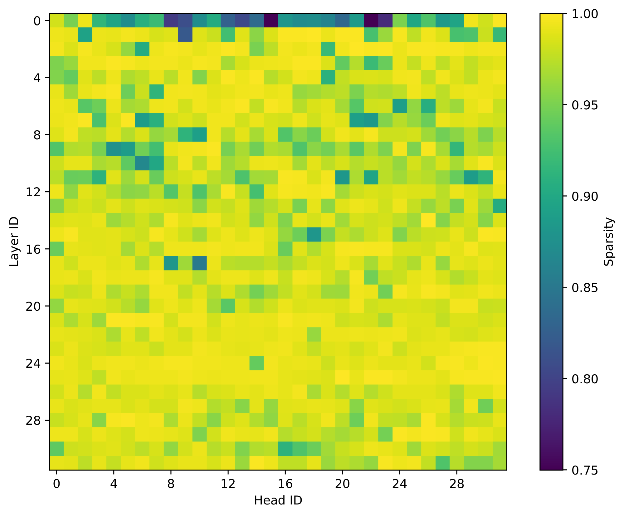
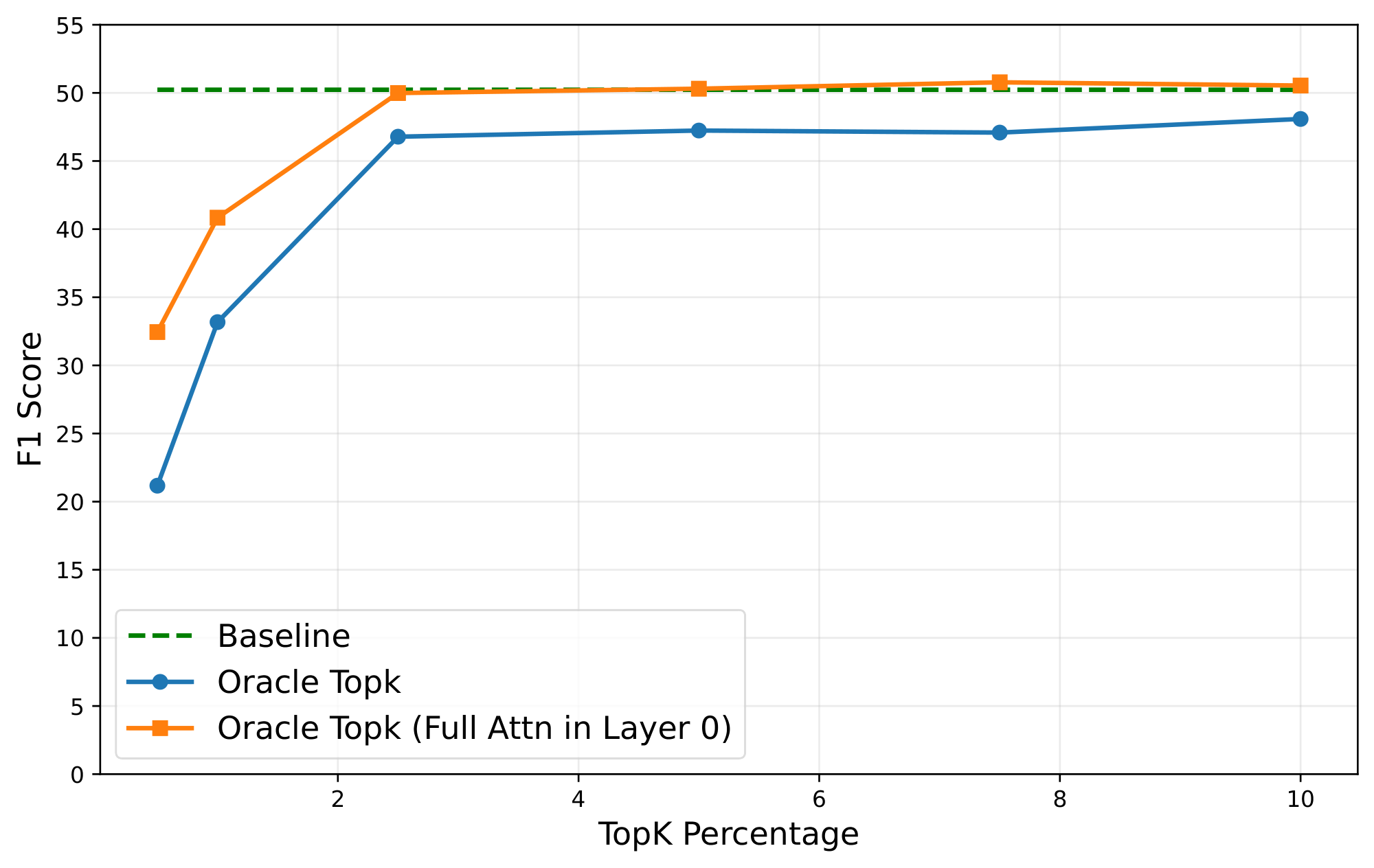
Kascade leverages two known observations: 1) the post-softmax attention scores are inherently sparse, and 2) the sparsity structure is stable across nearby layers. Figure 1 shows the sparsity inherent in attention operation. As shown, only 256 (about 10%) of the tokens contribute to over 95% of the softmax output. This is intuitive, as the softmax operation exponentially amplifies the relative magnitude of larger values compared to the smaller ones. Thus, if we have an oracle that determines the Top-$k$ tokens, which contribute most to the attention operation, we can get a very accurate approximation of the operation, at a fraction of the cost. Figure 2 shows the accuracy of Oracle Top-$k$ with varying values of $k$. As shown, with just 2.5% of tokens, one can recover almost the full accuracy of dense attention.

Figure 1 shows the sparsity inherent in attention operation. As shown, only 256 (about 10%) of the tokens contribute to over 95% of the softmax output.

These observations motivate our solution: we compute full attention, and identify Top-$k$ tokens, only on a subset of layers, which we call anchor layers, and reuse those Top-$k$ tokens to compute sparse attention in intermediate layers. In order to identify the best subset of anchor layers, we propose an automated dynamic programming scheme that maximizes cross layer similarity scores. This makes it easy to deploy Kascade on new models. We also observe that the Top-$k$ tokens vary across heads, and propose a head remapping technique when reusing these Top-$k$ tokens. We find this is critical for high accuracy. Therefore, by algorithmically choosing a good set of anchor layers, and being head-aware, Kascade achieves the best accuracy on AIME-24 among similar techniques for a given sparsity ratio.

Kascade incorporates design decisions based on low-level kernel implementation of the attention operation to get strong performance gains in both prefill and decode. For example, in the prefill attention kernel, the $QK^{T}$ operation is performed over tiles for maximizing parallelization and efficiency. As a result, consecutive tokens of a sequence in a Q-tile, share the same key tokens. Thus, Kascade performs the Top-$k$ selection at a tile level and not independently for each token. Kascade kernels are implemented in TileLang [15] and deliver substantial efficiency gains on H100s (up to $4.1 \times$ for decode attention compared to FlashAttention-3 baseline) with negligible impact on task accuracy across models and benchmarks.

In summary, we make the following contributions:

• Kascade introduces three efficient mechanisms: tiled top-K, head remapping and automatic anchor layer selection, for making sparse attention practical and accurate.
• Compared to previous techniques, Kascade achieves higher accuracy at the same Top-$k$. For example, in AIME-24, Kascade delivers substantially higher accuracy (8–10% absolute) compared to previous schemes with two different models at 10% Top-$k$.
• By automating anchor layer selection and head remapping, and with a performant kernel for H100s, we believe Kascade is the first kernel that makes it easy to deploy sparse attention for different models.
• On H100s, Kascade delivers up to $4.1\times$ faster performance than FlashAttention-3 decode kernel and up to $2.1\times$ faster performance than FlashAttention-3 prefill kernel, thereby ensuring significant performance gains while achieving comparable accuracy in long-context tasks.

2. BACKGROUND AND RELATED WORK

2.1 Scaled Dot-Product Attention

In scaled dot-product attention [16], each new token must attend to all previous tokens. Formally, for a query $\boldsymbol{q}_t \in \mathbb{R}^{d}$, corresponding to the current token, and key-value pairs $\boldsymbol{K}, \boldsymbol{V} \in \mathbb{R}^{N \times d}$ of past tokens, the attention output $\boldsymbol{y}$ is computed as:

$ \begin{align} \boldsymbol{p} &= \mathrm{softmax}\Bigl(\frac{\boldsymbol{q}_t \cdot \boldsymbol{K}^\top}{\sqrt{d}}\Bigr) \in \mathbb{R}^{N} \tag{1} \ \boldsymbol{y} &= \boldsymbol{p} \cdot \boldsymbol{V} \in \mathbb{R}^{d} \tag{2} \end{align} $

Here $N$ is the current sequence length, and $d$ is the hidden dimension. Equation 1 computes a weight for every token, and Equation 2 computes the output as a weighted sum of values in $\boldsymbol{V}$. As we'll see in Section 3.1, the $\boldsymbol{p}$ vector is sparse, and most of the weights are close to 0.

The above operation results in $O(N)$ computation and memory access per token, making attention the dominant contributor to latency in long-context inference.

2.2 Grouped Query Attention

In Multi-Head Attention [16], each head performs independent attention with its own learned projections of $Q, K, V$, and their outputs are concatenated and linearly transformed. Grouped Query Attention (GQA) [17] generalizes this formulation by allowing multiple query heads to share a common set of key-value projections, reducing memory bandwidth and improving efficiency in both training and inference. GQA is widely adopted in recent models, but imposes additional constraints on efficient implementation of sparse attention schemes, which we explore in Section 3.4.

2.3 Sparse Attention Methods

As we observed in Section 2.1, the attention operation is expensive because each token has to attend to all previous context tokens. To address this bottleneck, various sparse attention mechanisms have been proposed.

Fixed pattern sparsity approaches fix a connectivity pattern (e.g., sliding windows plus a small set of global tokens) [1, 2, 3, 4] and compute attention only over these tokens. Some models deploy sliding window attention on a subset of layers to limit the attention cost [18, 19]. However, these approaches work best when baked into the architecture before pre-training, as the model needs to learn to attend within this connectivity pattern; or require some amount of post-training.

Another class of techniques is workload-aware sparsity which primarily targets RAG like scenarios and limits the attention operation of document tokens to within the context of the same document [5, 6, 7, 8]. These techniques may also require some post-training to maintain accuracy, and they only optimize the prefill phase of inference.

The final family of approaches is dynamic sparsity, where a subset of k tokens is dynamically selected for the attention computation [20, 9, 10, 11, 12, 13, 14]. Selecting the best tokens efficiently is, however, an open research problem.

2.4 Cross-Layer Similarity in Attention

One key observation we use, described in Section 3.2, is that the sparsity patterns of attention weights exhibit strong correlations across neighboring layers. Prior works [21, 22, 23] have evaluated sharing full attention weights across layers, which we found to degrade accuracy.

Some recent works like OmniKV [24], TidaDecode [25], and LessIsMore [26] have also used this observation to design an approximate Top-$k$ attention scheme. OmniKV has a focus on reducing memory capacity requirements, and hence offloads the KV cache to the CPU. The benefit in memory capacity, however, comes at the cost of reduced performance because of CPU-GPU transfers. LessIsMore, built on top of TidalDecode, computes Top-$k$ indices on fewer layers chosen manually. A key challenge with these schemes is that there is not automated way to identify the anchor layers which makes it difficult to deploy to new models. These schemes use a shared set of Top-$k$ indices across all heads, while we find separate Top-$k$ indices for every key head to improve accuracy, as described in Section 3.5.

3. KASCADE

We now outline the various insights and techniques needed for a complete design and implementation of Kascade.

3.1 Oracle Top-$k$ Selection

We first ask a feasibility question: can we approximate attention using only a small subset of past tokens without losing task accuracy? Since the softmax operation in Equation 1 exponentially amplifies the relative magnitude of larger values compared to the smaller ones, it has an inherent sparsification. To exploit this sparsification, we define an Oracle Top-$k$, where we compute the attention, in Equation 2, only over $k$ tokens with the highest $\boldsymbol{p}$ values. Since computing these $k$ tokens requires the full softmax operation, we use the term Oracle, and this provides an accuracy upper bound.

Figure 1 confirms that the output of softmax is indeed sparse. For example, 95% of the total attention mass in almost all layers and heads is captured by the top 256 tokens. The only exception is layer 0, where the distribution is considerably flatter. Kascade therefore always computes full dense attention in layer 0 and applies sparsity only layer 1 onwards.

Figure 2 evaluates how aggressively we can sparsify while preserving task quality. We replace dense attention with Oracle Top-$k$ attention, and measure end-task accuracy (F1 on 2WikiMultihopQA [27] for Llama-3.1-8b-Instruct). Even at $k/N=2.5%$, Oracle Top-$k$ attention matches the accuracy of full attention. This shows that, if Top-$k$ can be estimated efficiently, the performance upside can be significant without compromising accuracy.

Kascade is designed to approximate this oracle efficiently. The next subsections address two challenges of doing this at runtime: (1) computing the Top-$k$ set without first materializing full attention, and (2) enforcing GPU-friendly sharing of Top-$k$ indices across tiles, layers, and heads for high throughput. We address (1) using cross-layer reuse of Top-$k$ indices and (2) using head remapping, tile-level pooling, and GQA-aware constraints.

3.2 Cross-Layer Similarity

We now ask whether we can avoid recomputing the Top- $k$ set independently in every layer by reusing it across nearby layers. For a query token $q$, let $P^{(l, h)}_q \in \mathbb{R}^N$ denote the post-softmax attention distribution, at layer $l$ and head $h$, where $N$ is the current sequence length. We define the layer attention distribution $P^l_q$ as the average of $P^{(l, h)}_q$ across all heads. We then define the Top-$k$ index set for token $q$ at layer $l$ as $I^l_q = topk(P^l_q, k)$.

To quantify how well the Top-$k$ set from one layer can be reused in another layer, we define a similarity score between two layers $a, b$ where $a < b$. For token $q$, we measure how much of layer $b$ 's oracle attention mass would be recovered if we were to force layer $b$ to use the Top-$k$ keys selected at layer $a$:

$ sim(a, b)q = \frac{\sum{i=1}^{k} P^b_q[I^a_q[i]]}{\sum_{i=1}^{k} P^b_q[I^b_q[i]]}, \tag{3} $

where $a > b$ and $|I^a_q| = |I^b_q| = k$

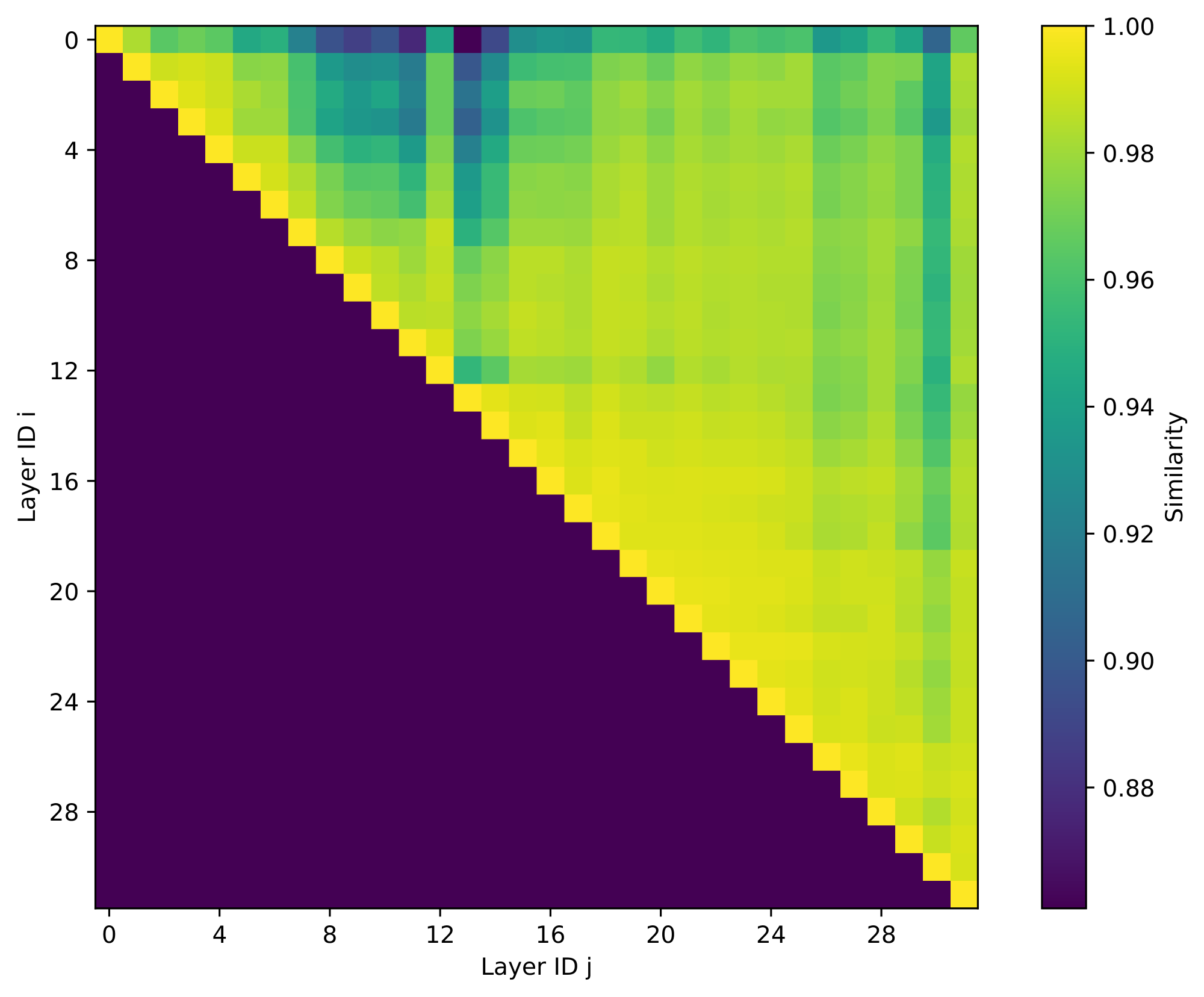
Values near 1 indicate that the identity of the high-importance keys is stable across layers. We compute this similarity for each query token in a prompt, then average across all tokens in that prompt. We then average again across a development set of multiple prompts to obtain a layer-by-layer similarity matrix $S \in \mathbb{R}^{L \times L}$, where $L$ is the total number of layers.

Figure 3 shows this cross-layer similarity matrix for Llama-3.1-8b-Instruct using MuSiQue as the development set, with $k=256$ (the average context length in MuSiQue is 2.3K). Most adjacent layer pairs achieve similarity scores close to 1. Similarity generally decays with layer distance, but remains high across short ranges. For example, similarity score of most nearby pairs stays above 0.98, meaning that more than 98% of the oracle Top-$k$ attention mass at layer $b$ is already covered by the Top-$k$ keys chosen at layer $a$.

With this observation, Kascade computes Top-$k$ indices on only a small set of anchor layers. These indices are then used to compute Top-$k$ attention on for the next few reuse layers.

3.3 Anchor Layer Selection

Given a budget for the number of anchor layers, we want to select the set of anchor layers, such that it maximizes the similarity between the chosen anchor layers and the corresponding reuse layers. Kascade performs this selection using the dynamic programming algorithm, shown in Algorithm 1 which uses the similarity matrix $S$ as input. To construct $S$, we evaluate the similarity scores $\text{sim}(a, b)_q$ (equation 2) for every token $q$ in a prompt, then take the minimum across tokens in that prompt, rather than the mean. This makes the score conservative and ensures that the similarity is determined by the worst token in a prompt. We observed that this resulted in a more robust anchor selection. We used $k=64$ for computing the similarity scores and found it to work well across experiments. The similarity matrix also incorporates the modifications described in Section 3.4, and Section 3.5.

**Require:** Similarity matrix $S$, budget $M$, layers $1\ldots L$
1: Initialize $\mathrm{dp}[][] = -\infty, \mathrm{path}[][]=0$
2: $\mathrm{dp}[1][1] = S[1][1]$
3: **for** $m=2 \to M+1$ **do**
4:     **for** $j=m \to L+1$ **do**
5:         $\mathrm{dp}[m][j] = \max_{i=m-1}^{j-1}(\mathrm{dp}[m-1][i] + \sum_{l=i}^{j-1} S[i][l])$
6:         $\mathrm{path}[m][j] = \mathrm{argmax}(.)$
7:     **end for**
8: **end for**
9: Backtrack on $\mathrm{path}[M+1][L+1]$ to recover $\{\ell\}$

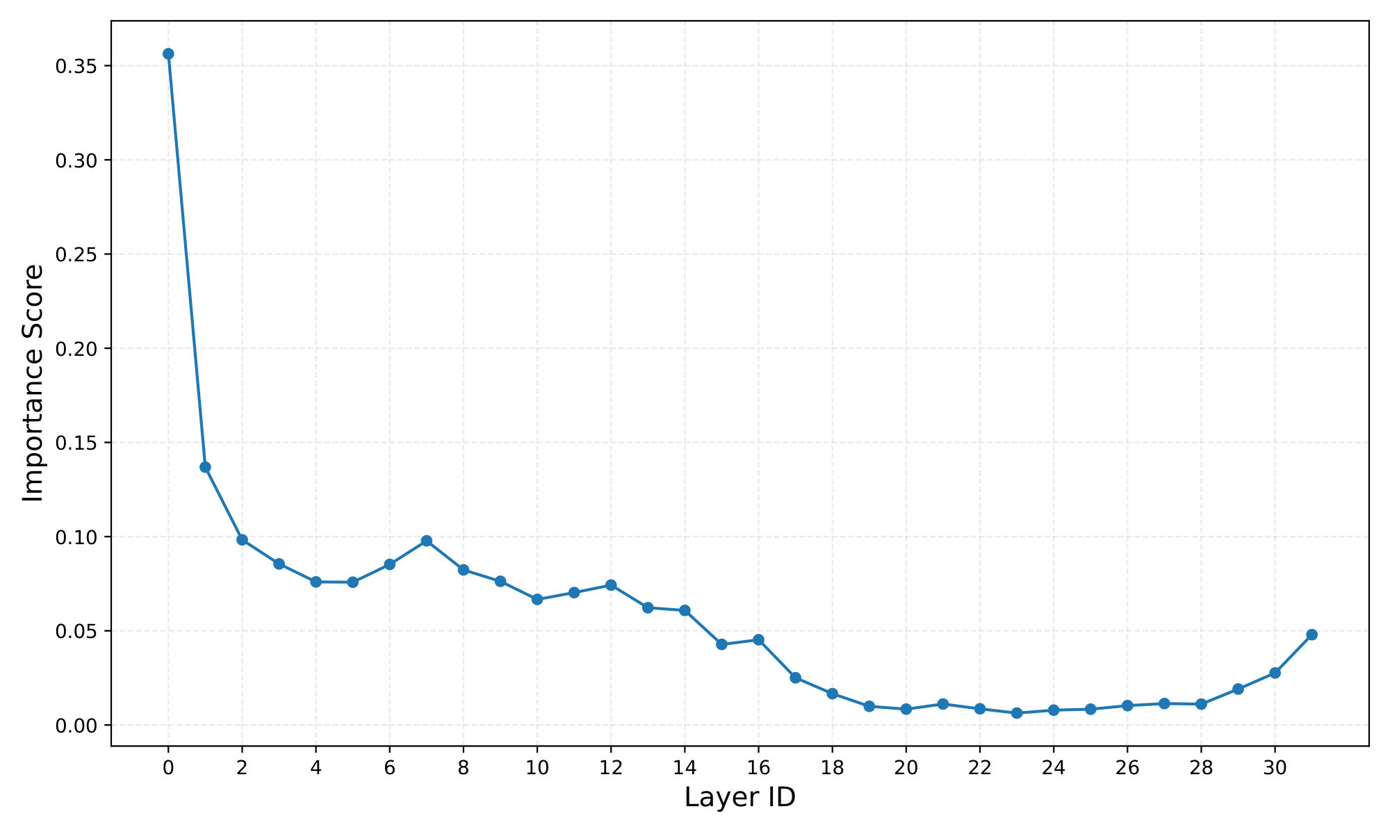
Prior work has observed that attention in deeper layers can be less important than attention in earlier layers [28]. We account for this observation by assigning each layer $l$ an importance weight $w_l$. If $\boldsymbol{x}^i_l$ and $\boldsymbol{y}^i_l$ are an (input, output) pair of attention at layer $l$, we define the importance score $w_l^i$ as:

$ w_l^i = 1 - \mathrm{CosineSim}(\boldsymbol{x}^i_l, \boldsymbol{y}^i_l) $

Intuitively, if attention barely changes the representation (high cosine similarity), that layer’s attention block matters less. The layer's weight is computed by aggregating this score over the same development set. The similarity matrix is then weighted by this importance measure.

Equation 1 computes a weight for every token, and Equation 2 computes the output as a weighted sum of values in $\boldsymbol{V}$.

Figure 4 shows the importance score for all layers in the Llama-3.1-8b-Instruct model showing a sharp decrease in importance of deeper layers.

We now discuss more enhancements to Kascade to incorporate finer attention implementation details.

3.4 Query pooling

Most modern LLMs use GQA [17] where multiple query heads share the same KV-heads. For efficiency and maximizing parallelization, the decode GQA attention kernels construct Q-tiles (for the $QK^T$ computation) by combining query values of all query heads sharing the KV-heads. Similarly, prefill kernels construct Q-tiles by combining consecutive tokens of the prompt as they all share the same prefix for the $QK^T$ operation. This allows batching of memory loads and reusing the fetched $K$ values across multiple queries, resulting in higher GPU utilization.

In order to maintain this efficiency, Kascade needs to ensure that all query tokens in a tile share the same Top-$k$ indices. We must thus construct a single ``pooled" attention score for these tiles during the Top-$k$ computation in the anchor layers. We consider two pooling strategies. Pre-Softmax pooling constructs a pooled query representation (by averaging the query vectors in a tile), and computes attention once using this pooled query. Post-Softmax pooling instead computes the full post-softmax attention distribution independently for each query in the tile, and then pools these attention distributions across the tile. We evaluate these pooling strategies in the Oracle setting in Figure 5. As shown, Post-Softmax pooling maintains accuracy even for large tiles, while Pre-Softmax pooling degrades as tile size increases.

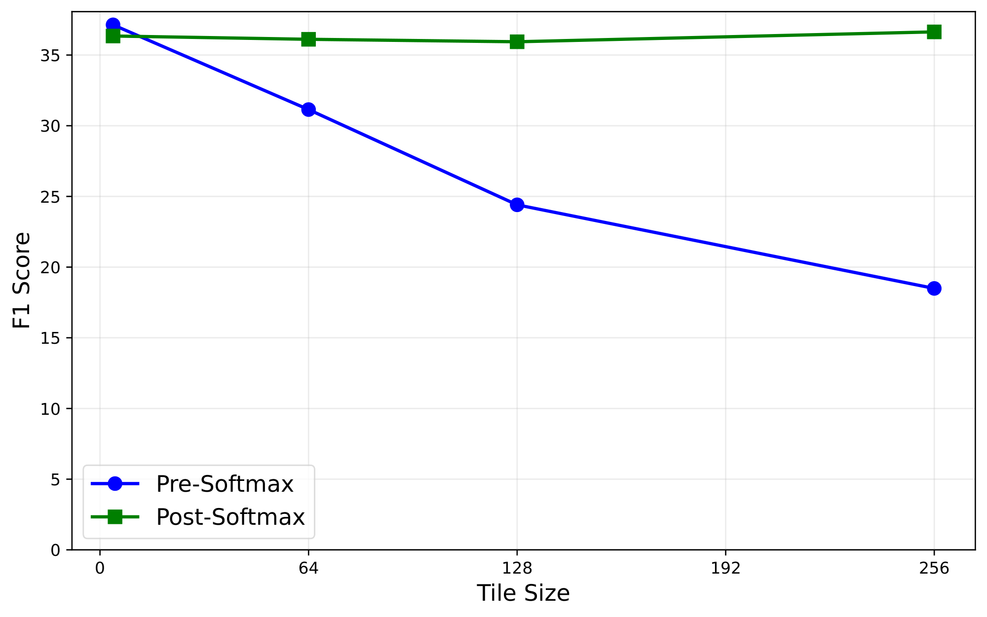
Based on these results, Kascade adopts Post-Softmax pooling. In decode, we pool only across the query heads that share a key head (GQA pooling). In prefill, we pool across full tiles of 128 queries (including the GQA grouping), which matches the tile size used in our dense FlashAttention-style baselines. This choice lets Kascade reuse a single Top-$k$ index set per GQA group in decode and per tile in prefill, and therefore aligns sparse attention with the kernel structure used by high-throughput implementations.

3.5 Head Remapping and Reuse

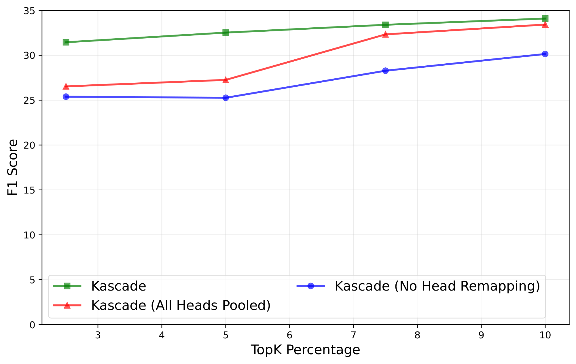
Kascade computes Top-$k$ indices at the granularity of a key head. Thus, each anchor layer will have $H$ Top-$k$ sets of indices, where $H$ is the number of key heads. This raises the question — which head's Top-$k$ index set in an anchor layer should be mapped to a given head in a corresponding reuse layer? One option is to perform a simple 1:1 mapping where the $i$ 'th heads in the anchor and reuse layers are mapped to each other. However, nothing in the transformer architecture requires that the head $i$ of one layer be similar to the head $i$ of another layer. We explore two strategies to handle this. One strategy is to use a shared set of Top-$k$ indices for all heads, by pooling the attention weights across all heads in a layer. This method will not account for any variation in the Top-$k$ indices across heads. In the second strategy, instead of forcing a single shared Top-$k$ across all heads, we build an explicit mapping from heads in each reuse layer to the most similar head in the corresponding anchor layer. For computing this mapping, we use the same similarity score defined earlier, but at a head level, and find a head mapping that maximizes the similarity. Note that this mapping can be a many-to-one mapping. A similar technique is proposed in [22] for reusing complete attention weights across layers.

Figure 6 compares these two strategies for Llama-3.1-8b-Instruct on MuSiQue across a range of Top-$k$ budgets. We observe that the head-remapping approach is consistently more robust, especially at smaller values of Top-$k$. Kascade therefore uses head remapping by default, but we also report results for the variant with a shared Top-$k$, across all heads, in Section 4.2 for completeness.

3.6 Efficient Kernel Implementation

We implement Kascade by modifying the FlashAttention [29] kernels for prefill and decode, in TileLang [15]. TileLang is a tile-level programming language for GPU kernels, which also takes care of various optimizations like pipelining, memory layouts and specialized instructions. We use both the original FA3, as well as TileLang FlashAttention kernels as our baseline in performance evaluations.

For intermediate reuse layers, we pass the Top-$k$ indices from the previous anchor layer, and the head mapping computed on the development set. During attention computation, we load the keys by consulting the Top-$k$ indices. The key loads that make a key tile are not contiguous, but given that each key is large, about 256 bytes, we do not notice any overhead with this. This is in contrast to claims by block sparse attention approaches [11, 13].

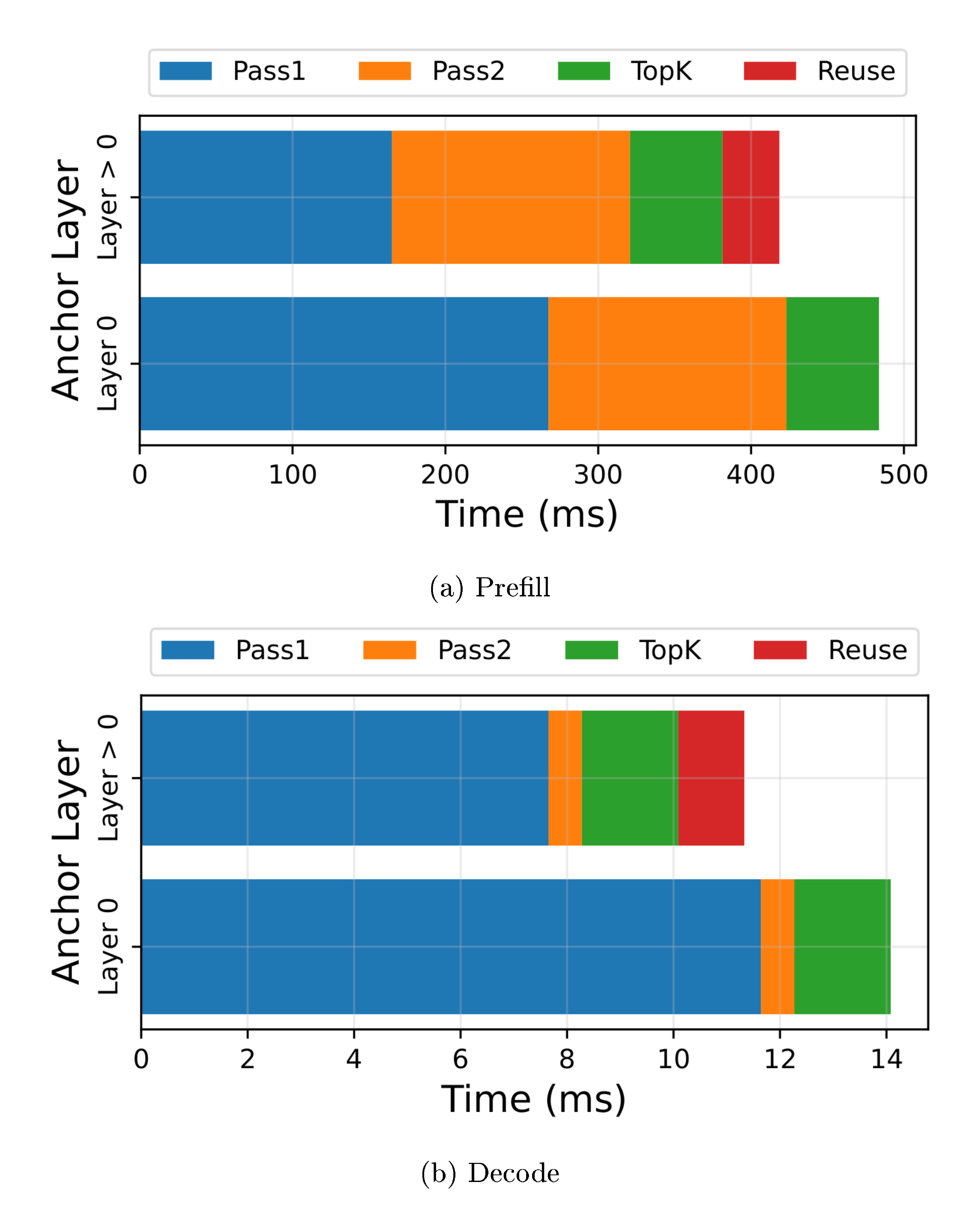
For anchor layers, we use a multi pass approach. Since we use Post-Softmax pooling, we need to first compute the post-softmax attention weights for each $q$ separately, and then pool them across a tile. We can not compute the pooled attention weights in one pass, since softmax operation requires knowing the full row sum.

• The first pass computes the full attention weight matrix $QK^T$, as well as the row sum vector ($\sum_{j=1}^{m} QK^T_{ij}$). This does about half the work of full attention. In decodes, we write out both these to HBM. In prefill, since the attention weight matrix is large, we only output the row sum vector.
• The second pass outputs the pooled post-softmax attention weights for each $Q$-tile. For decodes, we read the weights from the first pass, do a softmax, and pool. For prefill, we have to recompute the attention weights, but as we know the row sum vector, we can also compute the post-softmax weights and pool them.
• The third pass computes the Top-$k$ indices over the output of the second pass.
• In the final pass, we compute Top-$k$ attention similar to reuse layers.

For anchor layer 0, we need full dense attention as described in Section 3.1, so we compute dense attention in the first pass, and omit the last pass. Figure 8 shows the time split across these passes. We see that the recomputation in the second pass, for prefill, is a significant cost. We report performance numbers in Section 4.3

4. EVALUATION

:::

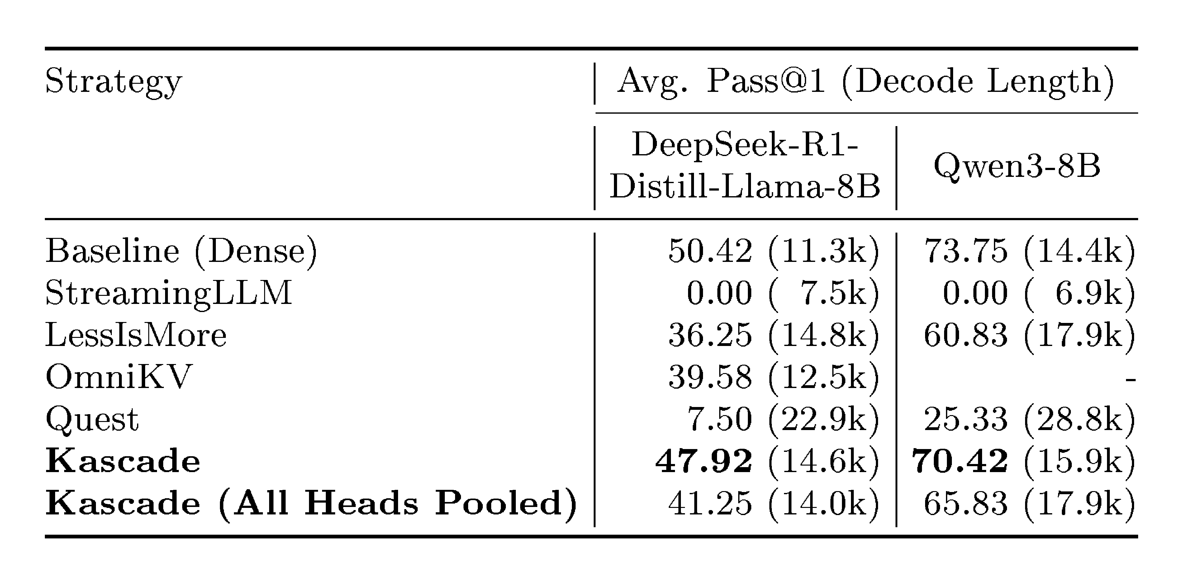
Table 2: Results on AIME-24. For StreamingLLM, sliding window is set to 30% with 4 sink tokens. For the Top-$k$ attention methods, Top-$k$ is set to 10%. Kascade gives the best accuracy across the board performing well even for decode heavy tasks. StreamingLLM fails to solve even a single question correctly.

:::

4.1 Setup

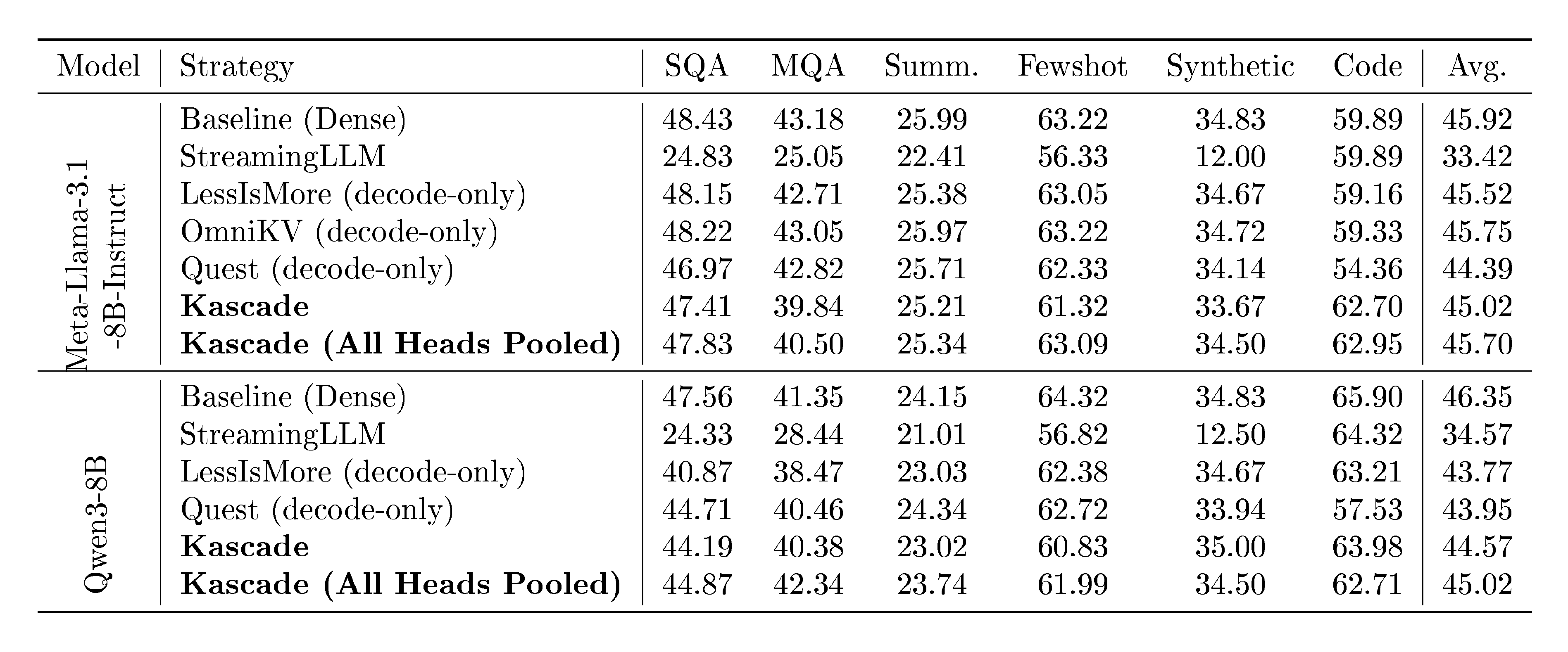
We evaluate Kascade on two popular long context benchmarks, LongBench and AIME-24. We also choose two, widely used, long context models for evaluation: Llama-3.1-8b-Instruct [30], and Qwen3-8b [31]. Both these models use GQA and can support up to 128k context length. For AIME-24 evaluations, instead of Llama-3.1-8b-Instruct, we use DeepSeek-R1-Distill-Llama-8b [32] which is a fine-tuned version of Llama-3.1-8b for reasoning tasks. The original Llama-3.1-8b-Instruct has very low baseline accuracy on AIME-24.

We do accuracy comparisons with dense attention, Quest [11], StreamingLLM [2], OmniKV [24] and LessIsMore [26]. We have implemented these algorithms in our own code-base, borrowing from any publicly available code. We also evaluate a variant of Kascade where we use a shared Top-$k$ across all heads (Section 3.5).

Kascade requires choosing a set of anchor layers. We use MuSiQue [33] as a development set and the anchor layer selection algorithm in Section 3.3 to choose the anchor layers. Llama-3.1-8b-Instruct has 32 layers, of which we choose 5 anchor layers, which are [0, 2, 8, 13, 14]. Qwen3-8b has 36 layers, of which we choose 5 anchor layers - [0, 2, 7, 14, 23]. For DeepSeek-R1-Distill-Llama-8b, we use the same layers as Llama-3.1-8b-Instruct, for Kascade, OmniKV and LessIsMore. OmniKV hasn't reported the filter layers for Qwen3-8b, so we remove it from Qwen3-8b comparisons.

For all accuracy results, we use a Top-$k$ of 10%, with a minimum size of 128. So, if the current sequence length is $L$, during decode, the number of Top-$k$ selected is,

$ k = \min(\max(0.1 \cdot L, 128), L) $

For Kascade, we also use the Top-$k$ in the prefill phase in a rolling manner, where each tile attends only to 10% of previous tokens. For Quest, OmniKV, and LessIsMore, prefill phase uses full attention. For StreamingLLM, given it is a weaker comparison, we use a sliding window size of 30% and 4 sink tokens. For AIME-24, we also show how the accuracy changes as we increase Top-$k$ to 20%.

4.2 Accuracy results

LongBench is composed of 21 long context tasks across 6 categories, covering multi-document QA, single-document QA, summarization, few-shot learning, code completion, and synthetic tasks. Almost all the tasks are prefill heavy, with very few decodes. All techniques except StreamingLLM and Kascade variants, do not use sparse attention in the prefill phase. Table 1 presents the results. We find that all techniques, including Kascade variants, perform very well on this benchmark. StreamingLLM is the only exception that doesn't perform well.

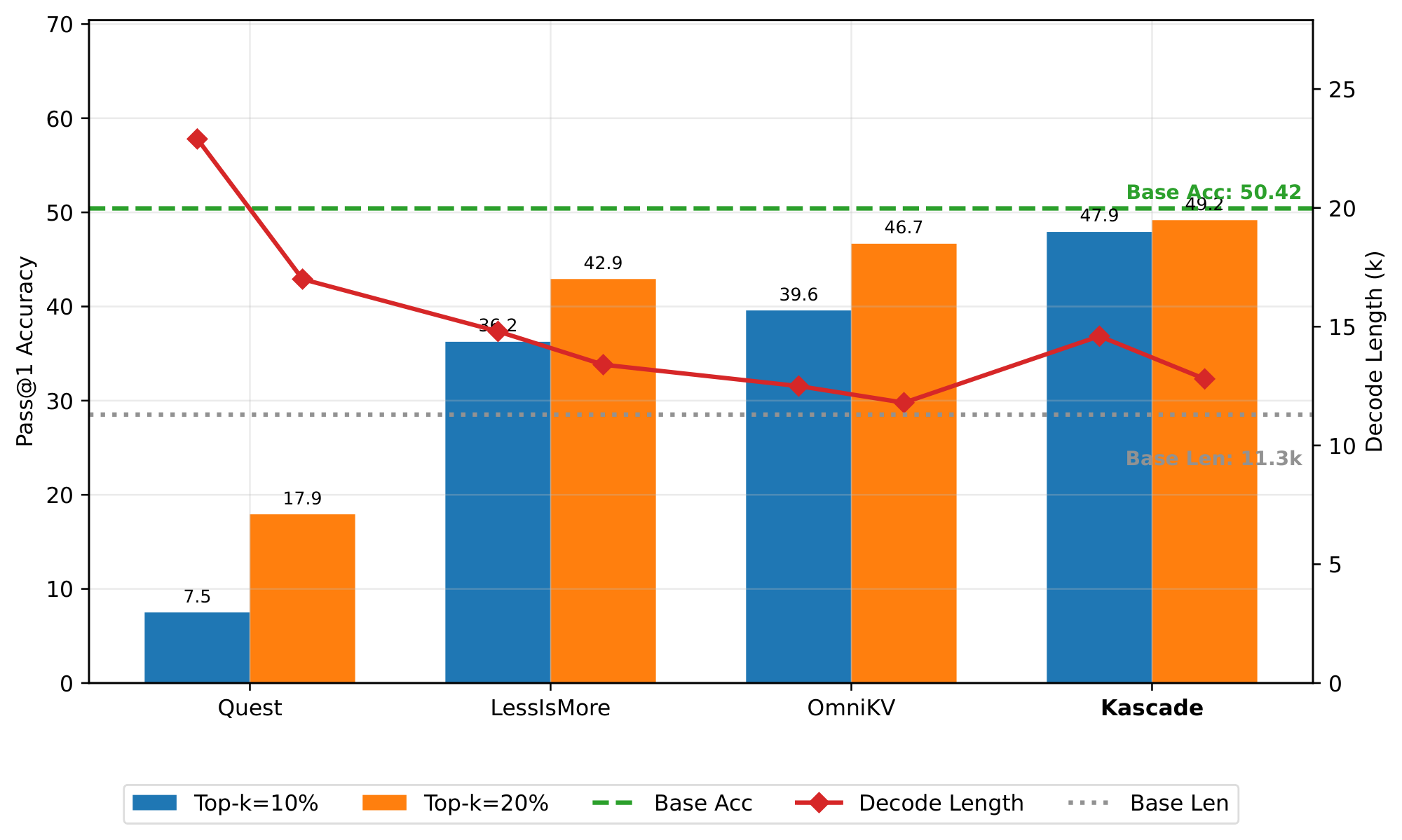
AIME-24 consists of 30 challenging mathematical problems, which typically require long chain-of-thought reasoning to get to the correct answer. Models that have not been trained for reasoning perform very poorly on these tasks. Table 2 presents the average of pass@1 score, across 8 runs, for each method. The attention patterns on these tasks can be complex, and we see that StreamingLLM is unable to solve any of the problems. We find that on this complex reasoning task, Kascade performs much better than other schemes. We also show the average decode length for each method. For Kascade, the average decode length is about 29% higher than baseline on DeepSeek-R1-Distill-Llama-8b, and 10% higher on Qwen3-8b. We also evaluate the shared Top-$k$ across all heads variant of Kascade, and it performs worse than default Kascade across both models, but better than other schemes.

In Figure 7, we evaluate the effect of increasing Top-$k$ to 20%. Kascade continues to have the highest accuracy and is very close to the baseline. The decode length also reduces, and is about 13% higher than baseline for Kascade.

4.3 Efficiency results

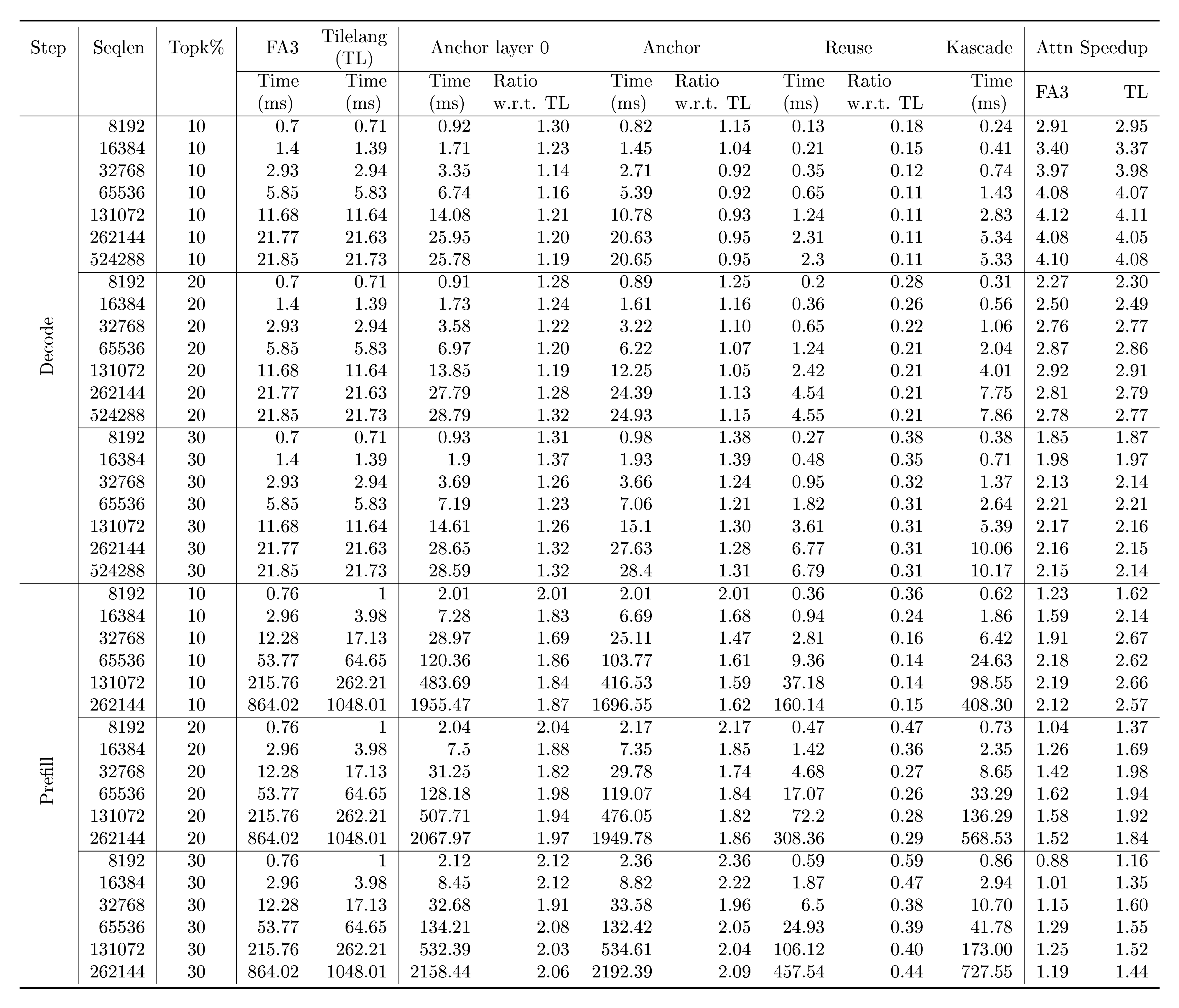
As discussed in Section 3.6, we implemented Kascade kernels in TileLang for both prefill and decode. We ran attention microbenchmarks on a single Nvidia H100 GPU, for varying context lengths. The settings used for attention are similar to that of Llama-3.1-8b-Instruct, with 32 total number of heads, 8 key heads, 128 head dimension, in fp16. For decode benchmarks we use a batch size of 64, except at context length 512k, which uses a batch size of 32 because of insufficient memory on a single gpu. Table 3 shows the results of these benchmarks on a combination of different Top-$k$ percentages and context lengths. We'll focus primarily on Top-$k$ percentage of 10%, and longer context lengths. We find that our reuse kernels see the expected speedup, and take about 10% of the time of full attention. Anchor layers take up more time, similar to the time of full attention. The first anchor layer additionally does dense attention, so takes even more time. Since we have 5 anchor layers, we compute the overall speedup accordingly. For decode phase, the speedup is about $4.1 \times$ wrt both FA3 and TileLang flashattention baselines, on Llama-3.1-8b-Instruct settings. For prefill phase, TileLang baseline kernels are about 20% slower than FA3. Further, as discussed in Section 3.6, our prefill kernels incur some extra costs in Top-$k$ computation, so our speedup wrt to TileLang is up to $2.6 \times$ and wrt to FA3 is up to $2.2 \times$. For Qwen3-8b settings, since the ratio of anchor layers is lower (5 of 36), we'd expect a higher speedup.

Figure 8 shows the time split of the multiple passes required for anchor layers. The time for layer $0$ is higher because it does dense attention in addition to computing Top-$k$ indices. Prefill speedup takes a hit primarily because of the recomputation of attention weights in the second pass of anchor layers.

5. CONCLUSION

We have presented Kascade as an efficient approximate Top-$k$ attention mechanism. It computes Top-$k$ indices in a subset of layers (anchor layers), and uses them to compute Top-$k$ attention in the next few reuse layers. To make this scheme accurate and practically deployable across models, we propose an automated way of choosing a good set of anchor layers, and make the algorithm head-aware. We also implement efficient kernels for this scheme for both prefill and decode, which requires sharing Top-$k$ indices across a tile of tokens. Kascade is able to achieve the best accuracy on AIME-24, among other training free sparse attention schemes, at a given sparsity ratio.

There are a few limitations of this work. First, this technique requires a development set to compute the anchor layers and head mappings. It is possible that this biases the technique towards the data in the development set. However, in the experiments we have done, we have found the selections to be robust to different datasets. Second, while Kascade reduces attention latency, it doesn't reduce the memory capacity requirements for attention. The KV caches of long sequences can be large and limit batch sizes which leads to reduced performance. Some attention works, therefore, target both capacity and latency benefits. Last, architectures which are trained with sparsity like [18, 19] will benefit less with this scheme.

REFERENCES

[1] Beltagy et al. (2020). Longformer: The long-document transformer. arXiv preprint arXiv:2004.05150.

[2] Xiao et al. (2023). Efficient streaming language models with attention sinks. arXiv preprint arXiv:2309.17453.

[3] Zaheer et al. (2020). Big bird: Transformers for longer sequences. Advances in neural information processing systems. 33. pp. 17283–17297.

[4] Jiang et al. (2024). Minference 1.0: Accelerating pre-filling for long-context llms via dynamic sparse attention. Advances in Neural Information Processing Systems. 37. pp. 52481–52515.

[5] Gim et al. (2024). Prompt cache: Modular attention reuse for low-latency inference. Proceedings of Machine Learning and Systems. 6. pp. 325–338.

[6] Yao et al. (2025). CacheBlend: Fast large language model serving for RAG with cached knowledge fusion. In Proceedings of the Twentieth European Conference on Computer Systems. pp. 94–109.

[7] Lu et al. (2024). Turborag: Accelerating retrieval-augmented generation with precomputed kv caches for chunked text. arXiv preprint arXiv:2410.07590.

[8] Dongyang Ma et al. (2025). Block-Attention for Efficient Prefilling. In The Thirteenth International Conference on Learning Representations. https://openreview.net/forum?id=7zNYY1E2fq.

[9] Singhania et al. (2024). Loki: Low-rank keys for efficient sparse attention. Advances in Neural Information Processing Systems. 37. pp. 16692–16723.

[10] Zhang et al. (2023). H2o: Heavy-hitter oracle for efficient generative inference of large language models. Advances in Neural Information Processing Systems. 36. pp. 34661–34710.

[11] Tang et al. (2024). Quest: Query-aware sparsity for efficient long-context llm inference. arXiv preprint arXiv:2406.10774.

[12] Yang et al. (2025). Lserve: Efficient long-sequence llm serving with unified sparse attention. arXiv preprint arXiv:2502.14866.

[13] Gao et al. (2024). Seerattention: Learning intrinsic sparse attention in your llms. arXiv preprint arXiv:2410.13276.

[14] Gao et al. (2025). SeerAttention-R: Sparse Attention Adaptation for Long Reasoning. arXiv preprint arXiv:2506.08889.

[15] Wang et al. (2025). TileLang: A Composable Tiled Programming Model for AI Systems. arXiv preprint arXiv:2504.17577.

[16] Vaswani et al. (2017). Attention is all you need. Advances in neural information processing systems. 30.

[17] Ainslie et al. (2023). Gqa: Training generalized multi-query transformer models from multi-head checkpoints. arXiv preprint arXiv:2305.13245.

[18] Team et al. (2024). Gemma: Open models based on gemini research and technology. arXiv preprint arXiv:2403.08295.

[19] Agarwal et al. (2025). gpt-oss-120b & gpt-oss-20b model card. arXiv preprint arXiv:2508.10925.

[20] Ribar et al. (2024). SparQ attention: bandwidth-efficient LLM inference. In Forty-first International Conference on Machine Learning. pp. 42558–42583.

[21] Ying et al. (2021). Lazyformer: Self attention with lazy update. arXiv preprint arXiv:2102.12702.

[22] Bhojanapalli et al. (2021). Leveraging redundancy in attention with reuse transformers. arXiv preprint arXiv:2110.06821.

[23] Xiao et al. (2019). Sharing attention weights for fast transformer. arXiv preprint arXiv:1906.11024.

[24] Jitai Hao et al. (2025). OmniKV: Dynamic Context Selection for Efficient Long-Context LLMs. In The Thirteenth International Conference on Learning Representations. https://openreview.net/forum?id=ulCAPXYXfa.

[25] Lijie Yang et al. (2024). TidalDecode: Fast and Accurate LLM Decoding with Position Persistent Sparse Attention. https://arxiv.org/abs/2410.05076.

[26] Lijie Yang et al. (2025). Less Is More: Training-Free Sparse Attention with Global Locality for Efficient Reasoning. https://arxiv.org/abs/2508.07101.

[27] Ho et al. (2020). Constructing A Multi-hop QA Dataset for Comprehensive Evaluation of Reasoning Steps. In Proceedings of the 28th International Conference on Computational Linguistics. pp. 6609–6625. https://www.aclweb.org/anthology/2020.coling-main.580.

[28] He et al. (2024). What matters in transformers? not all attention is needed. arXiv preprint arXiv:2406.15786.

[29] Shah et al. (2024). Flashattention-3: Fast and accurate attention with asynchrony and low-precision. Advances in Neural Information Processing Systems. 37. pp. 68658–68685.

[30] Grattafiori et al. (2024). The llama 3 herd of models. arXiv preprint arXiv:2407.21783.

[31] Yang et al. (2025). Qwen3 technical report. arXiv preprint arXiv:2505.09388.

[32] Guo et al. (2025). Deepseek-r1: Incentivizing reasoning capability in llms via reinforcement learning. arXiv preprint arXiv:2501.12948.

[33] Trivedi et al. (2022). MuSiQue: Multihop Questions via Single-hop Question Composition. Transactions of the Association for Computational Linguistics. 10. pp. 539–554.