Published as a conference paper at ICLR 2025

LANGUAGE MODELS ARE IMPLICITLY CONTINUOUS

Show me an executive summary.

Purpose and Context

Large Language Models (LLMs) like GPT and Llama are trained on discrete sequences of tokens—individual words or word fragments from a fixed vocabulary. However, the neural network architectures underlying these models are continuous mathematical functions. This research investigates a fundamental question: do LLMs internally treat language as discrete symbols (as humans do), or do they develop continuous representations that differ fundamentally from human language understanding? Understanding this has direct implications for improving model efficiency, interpreting model failures, and aligning AI systems with human reasoning.

Approach

The research team developed a mathematical extension of the Transformer architecture (the foundation of modern LLMs) called the Continuous Causal Transformer (CCT). This extension allows pretrained models to process inputs where tokens can have variable "durations" in time and where token embeddings can take intermediate values between known vocabulary words. Critically, this extension uses the existing weights from pretrained models without retraining, allowing the researchers to probe what these models have already learned. They tested six state-of-the-art models (Llama2, Llama3, Phi3, Gemma, Gemma2, and Mistral) across multiple experiments involving counting, arithmetic, and semantic reasoning.

Key Findings

The experiments reveal that LLMs exhibit continuous behavior in two fundamental ways:

*Time continuity*: When the duration of tokens is reduced (effectively making tokens occupy less "time" in the input sequence), models smoothly transition their outputs. For example, when asked to count four repetitions of the word "apple," reducing token durations causes the model to progressively predict 1, 2, 3, then 4 apples—as if it understands fractional tokens. In counting experiments across 200 test cases, models produced 190% more unique predictions than would be expected if they treated language discretely. Similar effects appeared in arithmetic: shrinking one number in a two-digit addition problem caused the model to treat it as a single digit, smoothly transitioning the answer.

*Space continuity*: When researchers created embeddings halfway between "apples" and "bananas" (vectors that don't correspond to any real word), models treated these meaningless interpolations as valid concepts with their own properties. For the prompt "Are ★ red?" (where ★ is an apple-banana interpolation), outputs smoothly transitioned from "yes" to "no." More remarkably, when asked "The most common colour for ★ is," several models predicted "green"—identifying an intermediate fruit concept with its own properties that exists nowhere in human language or the training data.

Implications

These findings challenge the assumption that LLMs process language similarly to humans. Models assign semantic meaning to concepts humans cannot comprehend, such as "half a token" or "the fruit between apples and bananas." This has three major implications:

First, for model development: the continuous nature of learned representations suggests new training approaches. Multiple similar sentences could potentially be processed simultaneously as interpolations, improving computational efficiency. However, this requires solving the challenge of disentangling outputs back to individual sentences.

Second, for model interpretability: current methods for understanding or controlling model behavior (such as removing biases by erasing specific representation regions) may have unintended consequences, since continuous interpolations mean that concepts overlap in complex ways. Work on "concept erasure" may inadvertently affect related concepts.

Third, for alignment and safety: if models reason about language fundamentally differently than humans, this mismatch could explain both unexpected capabilities (handling low-frequency inputs through interpolation) and unexpected failures (misunderstanding edge cases that seem clear to humans). Aligning AI systems with human values requires accounting for these representational differences.

Recommendations and Next Steps

Organizations deploying LLMs should recognize that these models may respond to inputs in ways that don't match human linguistic intuition, particularly for unusual or edge-case inputs. When debugging unexpected model outputs, consider whether continuous interpolation between concepts might explain the behavior.

For researchers, three directions warrant investigation: (1) developing training methods that exploit continuous representations for efficiency gains, (2) studying how continuous behavior affects model failures and edge cases, with direct relevance to safety, and (3) creating new interpretability tools that account for the continuous, non-human nature of learned representations rather than assuming discrete symbolic processing.

Before implementing interventions that modify model internals (such as bias removal or concept steering), test whether the intervention affects interpolated or related concepts, not just the target concept.

Limitations and Confidence

The experiments focus on specific types of prompts (counting, arithmetic, simple semantic questions) with six model families. While the consistency across models and tasks suggests the findings are general, the full scope of continuous behavior across all tasks and model architectures remains unknown. The research establishes that continuous representations exist and affect model outputs, but does not yet fully characterize when and how these representations influence real-world performance or where they might cause problems in deployed systems.

The mathematical framework (CCT) is sound and the experimental results are reproducible with provided code, giving high confidence in the core finding that modern LLMs are implicitly continuous. Lower confidence applies to predictions about practical applications—the efficiency gains from exploiting continuity and the safety implications both require further empirical validation before strong claims can be made.

Samuele Marro

1∗†{}^{1*\dagger}

, Davide Evangelista

{}^{2*}

, X. Angelo Huang

{}^{3}

, Emanuele La Malfa

{}^{4}

,
Michele Lombardi

{}^{2}

, Michael Wooldridge

{}^{4}

{}^{1}

Department of Engineering Science, University of Oxford, Oxford, UK

{}^{2}

Department of Computer Science, University of Bologna, Bologna, Italy

{}^{3}

Department of Computer Science, ETH Zurich, Zurich, Switzerland

{}^{4}

Department of Computer Science, University of Oxford, Oxford, UK

∗{}^{*}

These authors contributed equally.

†{}^{\dagger}

Corresponding author. Email: [email protected].

Abstract

Language is typically modelled with discrete sequences. However, the most successful approaches to language modelling, namely neural networks, are continuous and smooth function approximators. In this work, we show that Transformer-based language models implicitly learn to represent sentences as continuous-time functions defined over a continuous input space. This phenomenon occurs in most state-of-the-art Large Language Models (LLMs), including Llama2, Llama3, Phi3, Gemma, Gemma2, and Mistral, and suggests that LLMs reason about language in ways that fundamentally differ from humans. Our work formally extends Transformers to capture the nuances of time and space continuity in both input and output space. Our results challenge the traditional interpretation of how LLMs understand language, with several linguistic and engineering implications.

1. Introduction

Show me a brief summary.

In this section, the authors challenge the traditional view that language is fundamentally discrete by examining how Transformer-based language models process linguistic input. While language has historically been modeled as discrete sequences of tokens in both linguistics and computer science, the neural networks underlying modern LLMs are continuous, smooth function approximators, creating a fundamental tension between discrete data and continuous processing. The key insight is that training continuous models on discrete sequences does not necessarily mean the models treat language as discrete internally. By extending the Transformer architecture to accept continuous inputs without modifying pretrained weights, the authors demonstrate that state-of-the-art LLMs including Llama, Mistral, and Gemma implicitly learn continuous representations of language in both time and space. These continuous representations exhibit semantics that deviate significantly from human intuition, suggesting LLMs reason about language in fundamentally different ways than humans, with practical implications for more efficient pretraining strategies.

In linguistics and computer science, language is typically modelled as a discrete sequence of symbols: a sentence is a sequence of words, phonemes, characters, or tokens drawn from a finite vocabulary. This characterisation underpins both linguistics [1, 2, 3, 4] as well as classic and recent algorithmic approaches to language modelling [5, 6, 7].¹ In Machine Learning, a successful paradigm to model language is that of Large Language Models (LLMs, [8, 9]). In LLMs, language is modelled via an optimisation problem whose objective is to predict a word given its surrounding context [10, 11], though recent advancements fine-tune the models with procedures inspired by reinforcement learning [12, 13].

For completeness, a few notable works in linguistics and computer science model language as continuous: among the others, [14] and [15] model sentences as continuous entities in latent space, while recent approaches with quantum NLP represent meaning as a superstate of different words [16].

At their core, the architectures that model language, including feed-forward neural networks [17], Long-Short Term Memory Networks (LSTMs) [18, 19] and Transformers [20], approximate a discrete sequence of tokens with continuous smooth functions. However, training inherently continuous models on discrete sequences does not imply that the models themselves treat language as discrete.

This paper explores how the tension between discrete data and continuous function approximators is synthesised in Transformers-based Large Language Models [20]. To do so, we seamlessly generalise the Transformers architecture to support continuous inputs. This extension, which does not modify a model's weights or alter the architecture, allows the study of existing pretrained LLMs, including Llama [21], Mistral [22], and Gemma [23], with continuous input sequences.

By running experiments on state-of-the-art LLMs, we find that the language LLMs learn is implicitly continuous, as they are able to handle, with minor modifications, inputs that are both time continuous and spatial continuous. In particular, we formally show that the results obtained by extending pretrained LLMs to handle time continuous input strongly depend on a quantity, named duration, associated with each sentence. We also show in Section 4 that the semantics of this continuum significantly deviate from human intuition. Our results suggest that our intuition about human language can be misleading when applied to LLMs, as LLMs hold implicit representations of continuous sequences in unintuitive ways. Furthermore, these observations have practical consequences from an engineering perspective, as they suggest that it is possible to leverage the continuous representations of LLMs to pretrain them more efficiently.

Our code is available at https://github.com/samuelemarro/continuous-llm-experiments.

2. Related Work

Show me a brief summary.

In this section, the authors position their work within the broader landscape of continuous extensions to language models and transformers. While modern pretrained language models operate on discrete tokens, recent research has explored continuous-time transformers in domains like dynamical systems modeling and time series analysis, building on neural ODE frameworks. In natural language processing specifically, several approaches have combined transformers with neural ODEs to create time-continuous architectures, while spatial continuous extensions expand the embedding space beyond discrete token mappings, notably in diffusion language models. Additionally, researchers have studied continuous representations at the neuron and concept levels, showing that LLMs can map specific neurons to concepts and that certain models feature function vectors representing operations. The authors' contribution demonstrates that standard discretely-trained LLMs already exhibit continuous behaviors without requiring specialized continuous embedding training, as shown in prior work, and they provide an architecture-independent theoretical framework for studying these phenomena, revealing that concept interpolation occurs naturally and may complicate concept erasure approaches.

Modern state-of-the-art pretrained language models operate on a discrete number of tokens and do not handle continuous inputs directly. However, in other domains, extensions of classical Transformers [20] to time continuous inputs have been recently explored in tackling different problems. In modelling dynamical systems, [24] have proposed adding new regularisations to a classical transformer to create continuous behaviour in an attempt to improve upon existing time continuous models such as Neural ODEs [25, 26]. In time series modelling, [27, 28] further developed the ideas advanced by Neural ODEs by integrating time continuous transformers and, consequently, superseding other existing approaches such as Neural CDE [29] and Neural RDE [30].

Another line of work considers time continuous extension of language by processing it through networks combining the flexibility of classical Transformers with the mathematical interpretability of NeuralODEs, such as ODETransformer [31], CSAODE [32], TransEvolve [33], and N-ODE Transformer [34]. Several authors have also explored spatial continuous extensions of LLMs [35, 36, 37], where the embedding space is expanded to include vectors not directly mapped to specific tokens, thereby enhancing the representational power of the models. A broad class of Diffusion Language Models [38, 39, 40, 41, 42, 43] employs a similar concept, where the model generates elements not necessarily tied to individual tokens in the embedding space, thereby effectively incorporating spatial continuous extensions into language modelling.

Additionally, continuous representations in LLMs have been studied either in the context of concepts for which intuitive spectra exist [44, 45] or from a neuron-driven perspective [46]. In particular, our work can be seen as complementary to the latter: while the authors of [46] show that certain neurons map to specific concepts (which can then be steered), we show that such concepts exist even at the embedding level, and we offer a theoretical framework to study formally such phenomena in an architecture-independent manner.

Continuing the overview of related works, in [47] the authors remove concepts like biases by erasing the pertinent area that makes that concept emerge. Our work shows however that LLMs can interpolate between "overlapping" concepts: erasing an entire area might thus also affect other concepts, which represents an interesting research direction. Moreover, in [48] the authors show that some LLMs feature function vectors, which represent specific operations (e.g. sums), It is possible that some of the continuous behaviours in an LLM arise as function vectors.

Finally, our work can also be seen as a response to [49], which trains inherently continuous embeddings: we show that this process is not necessary, as even discretely trained LLMs show similar behaviours.

3. A Continuous Generalisation of Language Models

Show me a brief summary.

In this section, the authors challenge the traditional discrete view of language by proposing that sentences can be modeled as continuous-time functions, where each observed token represents a sample from an underlying stepwise constant function defined over continuous time intervals, with each token possessing a duration property. They formalize this by extending the standard Transformer architecture into a Continuous Causal Transformer (CCT) that replaces discrete summations in the attention mechanism with continuous integrals, allowing the model to process inputs at any real-valued timestep while preserving pretrained weights from existing models. Under the stepwise constant assumption, the integral simplifies to a duration-weighted sum that reduces to the classical discrete attention when all tokens have unit duration, proving that standard Transformers are special cases of CCT. This framework reveals that pretrained models implicitly encode temporal continuity and are invariant to time-shifting but sensitive to duration scaling, with the construction naturally extending to spatial continuity where intermediate embeddings between valid tokens can carry semantic meaning.

In this section, we propose the hypothesis that language can be seen as the discretisation of a spatio-temporal continuous function whose value corresponds to a valid token for any integer timestep. As we will show, this assumption allows us to define a continuous extension of the classical casual Transformer module, namely the Continuous Causal Transformer (CCT). The CCT accepts spatio-temporal continuous functions as input while including pretrained models on regular time- and space-discrete data as a special case. Moreover, we will formally discuss the implications of this construction, showing the basic results required to describe the experiments we presented later.

3.1 Time Continuity

Following classical approaches [50], we define a natural sentence as a sequence

{w1,w2,…,wT}⊂W\{ {\mathbf{w}}_1, {\mathbf{w}}_2, \dots, {\mathbf{w}}_T \} \subset \mathcal{W}

of tokens, sampled from an underlying distribution

p(w1,w2,…,wT)p({\mathbf{w}}_1, {\mathbf{w}}_2, \dots, {\mathbf{w}}_T)

, where each token

wt{\mathbf{w}}_t

only depends on previous timesteps, i.e.

p(w1,w2,…,wT)=p1(w1)∏t=2Tpt(wt∣w<t)p({\mathbf{w}}_1, {\mathbf{w}}_2, \dots, {\mathbf{w}}_T) = p_1({\mathbf{w}}_1)\prod_{t=2}^T p_t({\mathbf{w}}_t | {\mathbf{w}}_{<t})

, where we defined

w<t:=(w1,…,wt−1){\mathbf{w}}_{<t} := ({\mathbf{w}}_1, \dots, {\mathbf{w}}_{t-1})

. Moreover, given a continuous function

E:W→Rd\mathcal{E}: \mathcal{W} \to {\mathbb{R}}^d

that embeds any token

wt{\mathbf{w}}_t

as a

d

-dimensional vector

xt:=E(wt){\mathbf{x}}_t := \mathcal{E}({\mathbf{w}}_t)

, we name the push-forward distribution

p(x≤T):=E#p(w≤T)p({\mathbf{x}}_{\leq T}) := \mathcal{E}_\# p({\mathbf{w}}_{\leq T})

the distribution of natural sentences. Clearly, since the set

W\mathcal{W}

is inherently discrete, then the set

X=Rg(E)\mathcal{X} = Rg(\mathcal{E})

, i.e., the range of

E\mathcal{E}

, is a finite set, to which we refer as the space of valid embeddings. Indeed, in any classical formalisation of language, a sentence is considered to be finite both in time and space.

In this work, we hypothesise that any observed sentence

{xt}t=1T∼p(x≤T)\{ {\mathbf{x}}_t \}_{t=1}^T \sim p({\mathbf{x}}_{\leq T})

originates from the integer discretisation of a function

x(t){\mathbf{x}}(t)

, defined on the real interval

[0, T]

. Clearly, there exist infinitely many of these functions. In this section, we assume for

x(t){\mathbf{x}}(t)

the simplest, possible form: a stepwise constant function, defined as

where

1[as,bs](t)\mathbb{1}_{[a_s, b_s]}(t)

is the indicator function of the interval

a_s, b_s]

, whose value is 1 if

\in [a_s, b_s]

, 0 otherwise. For the intervals

{[a_s, b_s]\}_{s=1}^T

we assume that:

${[a_s, b_s]\}_{s=1}^T$ define a partition of the interval $[0, T]$ , i.e. {#assumption1}

$\in [a_s, b_s]$ for any $\dots, T$ . {#assumption2}

With this assumption, a sentence can be seen as a continuous flow of information, where the duration of each word is defined as the length of the interval defining it, i.e.

b_s - a_s

. Throughout the rest of this paper, we will refer to the duration of a token

xs{\mathbf{x}}_s

d_s := b_s - a_s

. A representation of this concept is summarised in Figure 1.

To be able to process time continuous inputs, we need an extension of the typical causal Transformer architecture, which we name Continuous Causal Transformer (CCT). We argue that any Transformer-based LLM can be seen as a discretisation of our CCT, and we propose a technique to modify the architecture of standard LLMs to handle stepwise-constant sentences as input, which represents the basis of our experiments in Section 4.

To prove our statement, we begin by considering the classical formulation of multi-head causal attention module, where the transformed output

{yt}t=1T\{ {\mathbf{y}}_t \}_{t=1}^T

associated with the sequence

{xt}t=1T\{ {\mathbf{x}}_t \}_{t=1}^T

is defined as:

where

Zt:=∑s′=1texp⁡(qtTks′d)Z_t := \sum_{s'=1}^t \exp \left(\frac{{\mathbf{q}}_t^T {\mathbf{k}}_s'}{\sqrt{d}} \right)

is a normalisation constant, and:

where

W^{(q)}

W^{(k)}

, and

W^{(v)}

are the attention matrices that are learned during training. Note that Equation 8 is equivalent to Equation 2 as long as the partition

Therefore, a continuous extension of Equation 2 can be simply obtained by substituting the sum with an integral, thus obtaining the continuous causal attention module

where

Zt:=∫0texp⁡(q(t)Tk(s)d)dsZ_t := \int_0^t \exp \left(\frac{{\mathbf{q}}(t)^T {\mathbf{k}}(s)}{\sqrt{d}} \right) ds

The multi-head version of Equation 4 is obtained by simply considering

H

independent copies of

y(t){\mathbf{y}}(t)

(namely,

{y1(t),…,yH(t)}\{ {\mathbf{y}}_1(t), \dots, {\mathbf{y}}_H(t) \}

), concatenating them and multiplying the result with a parameter matrix

W^{(o)}

Note that the learned matrices

W^{(q)}

W^{(k)}

W^{(v)}

, and

W^{(o)}

do not depend on the time discretisation (since they act on the feature domain of

xt{\mathbf{x}}_t

and

yt{\mathbf{y}}_t

). Consequently, we can use pretrained weights from any classical LLM.

To complete the construction of our CCT architecture, we remark that the Add&Norm scheme can be naturally re-used as it is, computing the final output

x~(t)\tilde{{\mathbf{x}}}(t)

as:

Finally, we observe that Equation 4 can be simplified by considering our stepwise-constant assumption for the language, as in Equation 1. Indeed, we show in Appendix A.2 that:

where

tˉ\bar{t}

is the only integer such that

\in [a_{\bar{t}}, b_{\bar{t}}]

, whose existence and uniqueness are guaranteed by (H1) and (H2). Note that Equation 8 is equivalent to 9 as long as the partition

{ [a_k, b_k] \}_{k=1}^T

is chosen so that each token has a uniform duration

d_k = 1

for all

\dots, T

, since in this case for any integer timestep

t

which is exactly Equation 9.

However, the CCT module is more general in the sense that it can easily handle arbitrarily stepwise constant functions, for example with non-uniform duration. Indeed, we can simply choose any partition of the interval

[0, T]

into sub-intervals satisfying condition §, and apply Equation 8 to compute the continuous transformed output

y(t){\mathbf{y}}(t)

. Interestingly, Equation 8 implies that, for a fixed input sentence

x(t){\mathbf{x}}(t)

, the output

y(t){\mathbf{y}}(t)

does not depends on the chosen partition

{ [a_k, b_k] \}_{k=1}^T

, but only on the durations

d_k

of each token. This suggests that our CCT shows shifting-invariance, i.e. the output does not change if the input gets shifted in time, as long as the shifted partition satisfies § and §. On the other hand, the CCT is not scale-invariant, since scaling will alter the token duration. These properties have been observed empirically in Appendix D.1.

3.2 Space Continuity

Note that, in our construction, we never explicitly used the fact that the range of

x(t){\mathbf{x}}(t)

is a subset of

X\mathcal{X}

, i.e. that any value of

x(t){\mathbf{x}}(t)

is an admissible token. This motivates the introduction of spatial continuous CCTs, where we consider a more general sentence in the form of Equation 1, where

xs{\mathbf{x}}_s

is not necessarily the embedding of a meaningful word

ws{\mathbf{w}}_s

. Note that our CCT model does not require any explicit modifications to be adapted to this setup.

Spatial continuity is particularly relevant when the value

xs∉X{\mathbf{x}}_s \notin \mathcal{X}

is obtained by interpolating between two meaningful tokens. Interestingly, we show in Section 4.3 that pretrained LLMs assign a semantic meaning to these intermediate embeddings, which results in something distinct from the two tokens which are used to compute the interpolation. Note that this is non-trivial and non-predictable, since the LLM never explicitly saw the majority of non-meaningful tokens as input during training, suggesting intriguing properties of the CCT architecture itself (which we aim to analyse more in-depth in future work).

To conclude, we remark that the stepwise constant assumption on the continuous language structure as in Equation 1 can be easily generalised to any other function structure for which a closed-form solution of the integral in Equation 4 can be obtained. This happens, for example, for any choice of piece-wise polynomial function defined over a partition of

[0, T]

, satisfying the assumptions (H1) and (H2). Testing the behaviour of the CCT architecture for other choices of

x(t){\mathbf{x}}(t)

is left to future work.

In the next sections, we will prove through several experiments that not only our proposed CCT model acts as a natural generalisation of classical Causal Transformer, recovering the same behaviour when a uniform discretisation of the domain into intervals of length 1 is considered, but also that the CCT seems to understand the concept of temporal fraction of a word.

4. Pretrained LLMs Are Implicitly Continuous

Show me a brief summary.

In this section, pretrained large language models are shown to exhibit implicit continuity in both temporal and spatial dimensions despite being trained exclusively on discrete data. When token durations are manipulated—such as compressing repeated words or entire sentences—models consistently respond as if perceiving fractional tokens, transitioning smoothly between counting one, two, three, or four items as duration varies, demonstrating understanding of temporal fractions that humans lack. Similarly, when embeddings are interpolated between semantically distinct tokens like "apples" and "bananas," models treat these intermediate representations as meaningful concepts with coherent properties: the interpolated entity is recognized as a fruit, and some models even assign it the color "green," suggesting knowledge of an intermediate fruit concept. These behaviors, observed across multiple model families including Llama, Gemma, and Mistral, reveal that LLMs construct continuous semantic representations fundamentally different from human language interpretation, challenging assumptions that model reasoning serves as a surrogate for human linguistic understanding.

In this section, we use our generalisation of LLMs to study the time continuous and space-continuous behaviours of pretrained LLMs. Thanks to our extension, we identify several novel properties of discretely trained models, such as the key role of duration as a semantic component and the existence of meaningful intermediate embeddings that do not map to any known token. Unless otherwise specified, our results hold for a wide variety of models, including Llama2-13B-Chat [51], Llama3-8B [21], Phi-3-Medium-4k-Instruct [52], Gemma-1-7B [53], Gemma-2-9B [23], and Mistral-7B [22].

4.1 Single-Token Time Continuity

We begin by studying how LLMs respond to variations in the time duration of a token. Consider the following input prompt to Llama3-8B:

In the sentence " $\underbrace{\texttt{\small apple}}_d_s = 1$ $\underbrace{\texttt{\small apple}}_d_s = 1$ $\underbrace{\texttt{\small apple}}_d_s = 1$ $\underbrace{\texttt{\small apple}}_d_s = 1$ ", how many fruits are mentioned?

The answer is naturally ``

4

", and we expect language models to reply similarly.² However, suppose that we reduce the duration of the portion of the sentence between double quotes, as defined in Section 3), i.e.,

Indeed, all the models we studied replied with "

4

In the sentence " $\underbrace{\scalebox{0.5}[1]{\texttt{apple apple apple apple}}}_{\sum \, d_s \; \in \; [1, 4]}$ ", how many fruits are mentioned?

As the duration of the four "apple" tokens varies, we expect the model to output either (1) "4", since the number of tokens has not changed or (2) nonsensical/unrelated tokens, since such an input would be out-of-distribution. Instead, Llama 3 returns an output that both is meaningful and differs from that of the original sentence. As shown in Figure 2, the output consists of each number from

1

4

, with peaks that vary with the token duration. In other words, the LLM interprets the sentence's content as if there were, respectively,

1

2

3

and

4

"apple" tokens.

From a linguistic perspective, the model returns outputs that, while reasonable, are hard to reconcile with the traditional interpretation of language in humans. LLMs naturally embody notions such as half a token (i.e., a token whose duration is not one time step), which humans lack.³ This suggests that LLMs interpret language differently compared to humans.

To obtain the same output from humans, one would modify the input to include instructions such as

\texttt{`Consider each apple word as half an apple'}

. We do not need to prompt an LLM with such instructions.

We quantitatively study this phenomenon by repeating this experiment on a dataset of 200 word counting tasks. In particular, we reduce the duration of all repeated tokens (in our example, 'apple') and measure how many unique applicable peaks we observe as the duration varies. For instance, if the word is repeated four times, as we vary the duration factor we expect the model to count, for different duration factors, 1, 2, 3, and 4 elements.⁴ A discrete interpretation of LLMs would predict that the model consistently predicts the same number (i.e. 4) regardless of the duration factor. Instead, we observe on average 190% more unique predictions. In other words, our results are incompatible with a discrete interpretation of the behaviour of LLMs. Refer to Appendix C.1 for a more in-depth overview of our methodology and results.

We treat 0 as an unexpected peak since the semantics of a zero-duration sentence are ill-defined.

In the next section, we stress the generality of this observation by applying the notion of time duration to multiple tokens and entire sentences.

4.2 Beyond Single-Token Time Continuity

A natural extension of token-level time continuity involves changing the duration of entire linguistic units.

We first study how LLMs behave when summing 2-digit numbers, where the duration of one of the addends is reduced. Consider the following input to Llama2-13B.⁵

We use Llama2 instead of Llama3 as the latter treats both digits as a single token.

The sum of 24 and $\underbrace{\texttt{1}}_d_{s_1}$ $\underbrace{\texttt{3}}_d_{s_2}$ is

As shown in Figure 3a, by shrinking the duration of the tokens "1" and "3", we observe that the model transitions from predicting "3" (i.e., the first token of the sum

24 + 13

) to "2" (i.e., the model progressively treats "13" as a single-digit number). Refer to Appendix C.3 for more examples of this behaviour across models and choices of numbers.

Additionally, we study how LLMs behave when we reduce the duration of entire sentences. For instance, consider the following passage, which is fed to Llama3-8B:

Alice goes to the shop. \ \ $\underbrace{\texttt{She buys a carton of milk.}}_d_{s_1}$ $\underbrace{\texttt{She buys an apple.}}_d_{s_2}$ \ $\underbrace{\texttt{She buys a potato.}}_d_{s_3}$ $\underbrace{\texttt{She buys a loaf of bread.}}_d_{s_4}$ \ How many items did Alice buy?

By reducing the duration of each sentence

{d_{s_1}, d_{s_2}, d_{s_3}, d_{s_4}\}

, we once again observe the model replying as if Alice bought 1, 2, 3 or 4 items (Figure 3b), which is consistent with our findings in the previous section. In particular, we observe on average 205% more unique predictions than what would be expected from a discrete interpretation of LLMs. Refer to Appendix C.2 for further data on this behaviour, which we observed to be present across all models.

There are thus reasons to believe that the notion of time continuity is innate in pretrained LLMs. Such a notion might emerge as a natural consequence of their nature as smooth function approximations, though further research in this direction is needed.

4.3 Space Continuity in Pretrained LLMs

In addition to time continuity, we study the nature of space continuity in LLMs.

In the NLP literature, it is widely known that the embeddings of semantically similar tokens tend to share some of their semantics, an observation often referred as the linear embedding hypothesis [54, 55]. However, thanks to our generalisation we discover that such hypothesis also holds for LLMs in the output space. In other words, inputs undergo a series of non-linear transformations to make an LLM predict the next word; yet, the intermediate embeddings and the output preserve the semantics of the interpolated inputs, with the region of the embedding space that, while not having any meaningful interpretation, are treated as proper concepts with well-defined properties.

Consider the following example for Llama3-8B:

Are ★ red?

In the previous example, ★ represents a linear interpolation of the embeddings of the "apples" and "bananas" tokens. Intuitively, such an interpolation does not have a proper semantics in human language (there is no such thing as "apple-bananas"). In fact, the interpolation does not map to the embedding of any known token (see Appendix C.4). Nevertheless, Llama3's output (as well as other LLMs') smoothly transitions between outputting "yes" and "no", as shown in Figure 4 (left). This behaviour is further confirmed by similar prompts like "Alice bought some ★ at the" (Figure 4 (right)). In other words, any interpolation between "apples" and "bananas" is treated as a grammatically correct part of a sentence.

While one may argue that the context plays a role in modelling the range of possible answers to these questions (e.g., in the first example "yes" and "no" are the only reasonable options), this interpretation only partially captures the nuances of LLMs' behaviour with space-continuous inputs. In fact, if we prompt the model with the following input:

Are ★ fruits?

the model always replies "yes", as reported in Figure 5 (left). Any interpolation of "apples" and "bananas" is indeed a valid fruit for the LLM. Additionally, for a subset of models (namely Llama 3, Gemma 1, Mistral, and partially Gemma 2), when we feed the input:

The most common colour for ★ is

we discover that the intermediate colour of "apples" and "bananas" is "green" (Figure 5), i.e., these Transformers hold the knowledge that there is a fruit in between "apples" and "bananas" whose colour is neither "red" nor "yellow". Refer to Appendix C.4 for more quantitative and qualitative results.

In short, LLMs assign a semantic meaning to their embedding space, but this meaning is neither trivial nor consistent with human intuition. These results challenge the assumption that the way LLMs interpret language is a surrogate of that of humans.

5. Implications

Show me a brief summary.

In this section, the authors argue that their findings reveal an incomplete understanding of language models and highlight two major implications. First, LLMs learn continuous representations of language that extend beyond discrete tokens, enabling new inference techniques such as parallel generation of sub-tokens through interpolations of semantically similar sentences, though applying this to training requires solving the non-trivial challenge of disentangling superposed tokens. Second, LLMs process language fundamentally differently from humans, as evidenced by their sensitivity to token duration and their assignment of meaning to embedding interpolations that lack human-interpretable semantics—behaviors unexplainable by data limitations alone. The authors advocate for an interdisciplinary effort combining linguistics and machine learning to study this "continuous language of LLMs," which could elucidate their performance on rare inputs, explain failures on human-meaningful edge cases, and ultimately improve both LLM capabilities and alignment with human reasoning.

Our results show that the current understanding of language models is incomplete. In this section, we highlight what we believe are promising implications of our findings.

LLMs learn a continuous representation of language.

While LLMs are mostly trained on discrete data, they learn representations that go beyond the meaning and interplay of each token. We thus argue that our generalisation of Transformers opens up to new inference techniques: for example, multiple sub-tokens can be generated in parallel as interpolations of sentences with similar templates but different semantics. The same intuition can be applied to training. Yet, it requires solving a non-trivial issue: tokens fed simultaneously and in "superposition" (e.g., an interpolation of multiple, semantically similar words) generate an output where each corresponding token should be disentangled and reassigned to its original sentence.

Language models treat language differently than humans.

Most of the examples reported in this paper contradict human intuition about language. Duration deeply affects a model's output in ways humans hardly grasp. Similarly, LLMs assign meaning to interpolations of embeddings even when such representations do not map to well-defined concepts. These behaviours represent a significant deviation from how humans reason about language, one that cannot be explained by a simple lack of data. We believe that the field of linguistics, alongside that of Machine Learning, should embrace the challenge of studying the continuous language of LLMs, synthesising classic tools from linguistics and deep learning. For instance, the notion of space continuity is deeply intertwined with how LLMs interpret language: we believe that our generalisation of Transformers can help us better understand the strong performance of LLMs on low-frequency inputs, as well as explain why they fail on edge cases that are semantically meaningful to humans.

Overall, our findings suggest that understanding more in-depth the continuous nature of LLMs can both improve their performance and align their representations with human reasoning.

6. Conclusion

Show me a brief summary.

In this section, the authors conclude that they have introduced a generalization of causal Transformers enabling the study of how pretrained LLMs respond to continuous inputs, revealing fundamental differences between how LLMs and humans process language. By characterizing time and space continuity, they demonstrate that LLMs assign complex semantic meanings to interpolations of embeddings that have no meaningful interpretation in human language and treat token duration as a key semantic property. These findings indicate that the conventional discrete understanding of LLMs is incomplete, as these models learn continuous representations that diverge from human linguistic intuition. The authors express hope that investigating the continuous behavior of LLMs will provide deeper insights into the language of Large Language Models, with significant implications for both the field of linguistics and the design of future LLM architectures.

In this paper, we introduce a generalisation of causal Transformers to study how pretrained LLMs respond to continuous inputs. We characterise the notions of time and space continuity, which we use to show that the language LLMs learn diverges from that of humans. In particular, LLMs assign complex semantic meanings to otherwise meaningless interpolations of embeddings and treat duration as a key property of their language. These results suggest that our traditional understanding of LLMs is incomplete.

We hope that, by studying the continuous behaviour of LLMs, future work will be able to shed further insight into the language of Large Language Models, with implications for both linguistics and LLM design.

Acknowledgements

Show me a brief summary.

In this section, the authors acknowledge the financial and institutional support that made their research possible, as well as the individuals who contributed through discussion and collaboration. The work received funding from the EPSRC Centre for Doctoral Training in Autonomous Intelligent Machines and Systems (grant EP/Y035070/1), alongside support from Microsoft Ltd and the Collegio Superiore di Bologna. Additionally, one of the authors, Emanuele La Malfa, received specific support from the Alan Turing Institute. Beyond institutional backing, the authors express gratitude to Aleksandar Petrov and Constantin Venhoff for engaging in insightful discussions that presumably helped shape or refine the research. This acknowledgement highlights the collaborative nature of academic work, recognizing both the material resources necessary for conducting research on continuous causal transformers and the intellectual contributions from peers that enriched the study's development and theoretical framework.

This work was supported by the EPSRC Centre for Doctoral Training in Autonomous Intelligent Machines and Systems n. EP/Y035070/1, in addition to Microsoft Ltd and the Collegio Superiore di Bologna. Emanuele La Malfa is supported by the Alan Turing Institute. We would like to thank Aleksandar Petrov and Constantin Venhoff for their insightful discussions.

A. Detailed Derivation of Section 3

Show me a brief summary.

In this section, the authors provide a detailed mathematical derivation for extending discrete causal transformers to their continuous counterpart. They begin by recapping how classical causal attention mechanisms compute output matrices through queries, keys, and values with a causal mask that ensures each output depends only on past or present inputs. The key insight is that the discrete attention formula can be rewritten as a weighted sum over tokens, where the weights depend on exponentially scaled inner products of query and key vectors. By treating the discrete sum as a Riemann approximation of an integral, the authors derive the continuous formulation where tokens have arbitrary durations instead of fixed unit lengths. The critical result is that the continuous attention output at time $t$ equals a weighted sum over all tokens, where each token's contribution is scaled by its duration, yielding an elegant closed-form expression that generalizes discrete transformers while preserving their computational structure.

A.1 A Recap on Discrete Transformer

In this section, we briefly recall how classical causal transformers work. Let

\in {\mathbb{R}}^{T \times d}

be the matrix whose rows are

xtT{\mathbf{x}}_t^T

. Then, each head of a causal attention mechanism computes a matrix

\in {\mathbb{R}}^{T \times d}

, such that:

where

\in {\mathbb{R}}^{T \times d_k}

\in {\mathbb{R}}^{T \times d}

are the queries, the keys, and the value, respectively, while

\in {\mathbb{R}}^{T \times T}

is the causal attention mask, which is introduced to ensure that each row

ytT{\mathbf{y}}_t^T

Y

only depends on observations

xs{\mathbf{x}}_s

with

\leq t

. The matrices

Q

K

V

are defined as:

where

W^{(q)}

W^{(k)}

, and

W^{(v)}

are the attention matrices that are learned during training, while the causal attention mask

M

is defined as:

The multi-head version of this causal attention mechanism typically used in modern architecture is obtained by computing

H

independent versions

{Y1,…,YH}\{ Y_1, \dots, Y_H \}

of Equation 10, and defining a learnable matrix

W(o)∈RdH×dW^{(o)} \in {\mathbb{R}}^{dH \times d}

, which combines them to obtain a single transformed observation matrix:

A continuous version of a multi-head attention network can be simply obtained by considering Equation 10 on a single timestep

\in [0, T]

. Indeed, it can be rewritten as:

where:

Consequently,

\begin{align} \begin{split} \text{softmax} \left(\left[\frac{QK^T}{\sqrt{d}} + M \right] _{t, s} \right) &\propto \exp \left(\left[\frac{QK^T}{\sqrt{d}} \right] _{t, s} \right) \cdot \exp \left[M \right] _{t, s} \\ &= \begin{cases} \exp \left(\frac{{\mathbf{q}}_t^T {\mathbf{k}}_s}{\sqrt{d}} \right) \quad &\text{if } s < t, \\ 0 &\text{otherwise}, \end{cases} \end{split} \end{align}\tag{16}

💭 Click to ask about this equation

(16)

Where

qtT{\mathbf{q}}_t^T

and

ks{\mathbf{k}}_s

are the

t

-th and the

s

-th rows of

Q

and

K^T

, respectively. Altogether, the above equations imply that:

where

Zt:=∑s′=1texp⁡(qtTks′d)Z_t := \sum_{s'=1}^t \exp \left(\frac{{\mathbf{q}}_t^T {\mathbf{k}}_s'}{\sqrt{d}} \right)

is a normalisation constant. The above formula is then used in Section 3 to define CCT.

A.2 Derivation of Equation 8

We recall that:

\begin{align} & {\mathbf{q}}(t) = W^{(q)} {\mathbf{x}}(t) = \sum_{k=1}^T W^{(q)} {\mathbf{x}}_k \mathbb{1}_{[a_k, b_k]}(t), \tag{18} \\ & {\mathbf{k}}(t) = W^{(k)} {\mathbf{x}}(t) = \sum_{k=1}^T W^{(k)} {\mathbf{x}}_k \mathbb{1}_{[a_k, b_k]}(t), \tag{19} \\ & {\mathbf{v}}(t) = W^{(v)} {\mathbf{x}}(t) = \sum_{k=1}^T W^{(v)} {\mathbf{x}}_k \mathbb{1}_{[a_k, b_k]}(t). \tag{20} \end{align}

💭 Click to ask about this equation

(18)(19)(20)

Consequently,

\begin{align} \begin{split} {\mathbf{y}}(t) &= \int_0^t \frac{1}{Z_t} \exp \left(\frac{{\mathbf{q}}(t)^T {\mathbf{k}}(s)}{\sqrt{d}} \right) {\mathbf{v}}(s) ds \\ &\overset{(20)}{=} \int_0^t \frac{1}{Z_t} \sum_{k=1}^T \exp \left(\frac{{\mathbf{q}}(t)^T {\mathbf{k}}(s)}{\sqrt{d}} \right) W^{(v)} {\mathbf{x}}_k \mathbb{1}_{[a_k, b_k]}(s) ds \\ &= \sum_{k=1}^T \int_{a_k}^{b_k} \frac{1}{Z_t} \exp \left(\frac{{\mathbf{q}}(t)^T {\mathbf{k}}(s)}{\sqrt{d}} \right) W^{(v)} {\mathbf{x}}_k ds \\ &\overset{(19)}{=} \sum_{k=1}^T \frac{1}{Z_t} W^{(v)} {\mathbf{x}}_k \int_{a_k}^{b_k} \exp \left(\frac{{\mathbf{q}}(t)^T \sum_{k'=1}^T W^{(k)} {\mathbf{x}}_{k'} \mathbb{1}_{[a_{k'}, b_{k'}]}(s)}{\sqrt{d}} \right) ds \\ &= \sum_{k=1}^T \frac{1}{Z_t} W^{(v)} {\mathbf{x}}_k \int_{a_k}^{b_k} \exp \left(\frac{{\mathbf{q}}(t)^T W^{(k)} {\mathbf{x}}_{k}}{\sqrt{d}} \right) ds \\ &\overset{(18)}{=} \sum_{k=1}^T \frac{1}{Z_t} W^{(v)} {\mathbf{x}}_k \exp \left(\frac{\left(\sum_{t' = 1}^T W^{(q)} {\mathbf{x}}_{t'} \mathbb{1}_{[a_{t'}, b_{t'}]}(t) \right)^T W^{(k)} {\mathbf{x}}_{k}}{\sqrt{d}} \right) \int_{a_k}^{b_k} ds \\ &= \sum_{k=1}^T \frac{1}{Z_t} W^{(v)} {\mathbf{x}}_k \exp \left(\frac{\left(W^{(q)} {\mathbf{x}}_{\bar{t}} \right)^T W^{(k)} {\mathbf{x}}_{k}}{\sqrt{d}} \right) (b_k - a_k) \\ &= \sum_{k=1}^T \frac{1}{Z_t} \exp \left(\frac{{\mathbf{q}}_{\bar{t}}^T {\mathbf{k}}_k}{\sqrt{d}} \right) {\mathbf{v}}_k d_k, \end{split} \end{align}\tag{21}

💭 Click to ask about this equation

(21)

which proves Equation 8.

B. Experimental Setup

Show me a brief summary.

In this section, the authors describe how to implement Continuous Causal Transformers (CCTs) by modifying standard transformers to accept arbitrary embeddings instead of tokens, support floating-point positional indices, and use custom floating-point attention masks. The key insight is that discretizing the integral in Equation 4 using Euler's method is equivalent to regular attention with carefully chosen coefficients, where the duration between samples affects their weights—specifically, samples farther apart receive higher weights proportional to their interval length. Practically, a sequence with durations and embeddings is fed by passing embeddings directly, defining positions cumulatively without gaps, and encoding durations through the discretization formulae. For experiments, the authors study logits directly without generation hyperparameters like temperature or top-k, implementing these modifications using HuggingFace, which natively supports custom embeddings and attention masks while requiring minimal adaptation for floating-point positions.

We now describe the shared aspects of our experiments.

B.1 Implementing a CCT

CCTs can be implemented with little effort by starting with the implementation of a regular transformer and applying three modifications:

Modifying it so that it accepts arbitrary embeddings, rather than only tokens;
Modifying it so that positional indices can be floating points, instead of only integers;
Adding support for custom floating-point attention masks.

In our experiments, we used HuggingFace, which natively supports 1. and 3. and can be easily adapted to support 2.

Note that the last modification is necessary in order to support non-standard durations. In fact, the Euler discretisation of the integral in Equation (4) is equivalent to regular attention with carefully chosen attention coefficients.

Proof

The discretisation of Equation (4) is, assuming that we have

n

samples at positions

p1,…,pnp_1, \dots, p_n

, which represent the value of a piecewise constant function defined over the intervals

p_1], (p_1, p_2], \dots, (p_{n-1}, p_n]

with

p_0 = 0

. In other words, if we are using multiplicative attention coefficients, the discretisation is equivalent to applying attention coefficients of the form

p_i - {p_i - 1}

. Intuitively, this means that the further apart two samples are, the higher the weight of the latter sample.

Note that for additive coefficients we can simply bring

p_i - p_{i-1}

inside the exponential:

which is equivalent to an additive coefficient of

p_i - p_{i - 1}

In Practice

At the implementation level, a sequence of

n

elements with durations

d1,…,dnd_1, \dots, d_n

and embeddings

e1,…,ene_1, \dots, e_n

is fed to the extended transformer as follows:

The embeddings $e1,…,ene_1, \dots, e_n$ are fed directly, rather than feeding the sequence as tokens and mapping them to embeddings;
The positional encodings are defined such that no "holes" are left in the piecewise constant function. In other words, the position $p_i$ is defined as $pi=∑j=1i−1djp_i = \sum_{j = 1}^{i - 1} d_j$ ;
The durations are encoded using the formulae described in Equations (22) and (23).

B.2 Experiment Hyperparameters

Since we study the logits, we do not use any typically generation-related hyperparameters (e.g. temperature and top-k). Aside from those described in Appendix B.1, we do not perform any other modification. Experiment-specific parameters are reported in the respective subsections of Appendix C.4.

C. Continuity - Full Results

Show me a brief summary.

In this section, the authors present comprehensive experimental results demonstrating that large language models exhibit continuous behavior that contradicts discrete interpretations of language processing. Through single-token continuity experiments, they show that shrinking token durations causes models to produce varying predictions with multiple unique peaks rather than constant outputs, with observed peak frequencies averaging 2.90 times higher than counterfactual expectations across six models. Event counting experiments similarly reveal that duration manipulation produces 3.28 times more peaks than discrete models would predict. Arithmetic sum experiments demonstrate that when numbers are shrunk, models shift predictions toward answers corresponding to single-digit interpretations in 87.82% of cases. Space continuity experiments through embedding interpolation reveal that intermediate points between token pairs (like "apples" and "bananas") yield semantically meaningful but non-discrete outputs, with 20.79% of interpolations producing probability values outside the range defined by the endpoint tokens, indicating emergent intermediate concepts that challenge human linguistic intuition.

C.1 Single-Token Continuity

C.1.1 Qualitative Results

For single-token continuity, we shrink the subset of considered tokens with a coefficient in the range

[0.1, 1]

Since the LLMs do not necessarily return a numeric value, all of the queries were wrapped with a prompt to coax the model into doing so. The template for our prompts is thus:

Question: In the sentence "[REPEATED WORDS]", how many times is [CATEGORY] mentioned? Reply with a single-digit number\\Answer:

For Gemma 1, Llama 2 and Mistral we used a slight variation, since they did not return a numeric output:

Question: How many [CATEGORY] are listed in the sentence "[REPEATED WORDS]"? Reply with a single-digit number\\Answer:

We used variations of these two prompts throughout most of this paper. See the source code for further information. Alongside apples, we also tested the same prompt with the word ``cat" (category: "animal") and "rose" (category: "flower"). See Figure 6, Figure 7, and Figure 8 for full results.

C.1.2 Quantitative Results

We reduce the duration of all the steps (following the procedure described in Appendix B) and measure the time sensitivity, i.e. the number

k

of unique applicable token peaks divided by the expected number of peaks

n

. For instance, if there are 4 steps, we expect to see peaks for 1, 2, 3, and 4. Our dataset is composed of 200 sentences with the same template as Appendix C.1.1 Note that, for some sentence+tokenizer combinations, a single word might be split into multiple tokens. As our analysis focuses on single-token words, we ignore such cases. Refer to Table 1 for the percentages of considered results for each model.

We define a unique relative peak as a situation where, for at least one duration factor, a certain class is the top prediction. For example, if by varying the duration factor the top class becomes 1, then 2, then 1 again, then 3, the unique relative peaks will be

{1, 2, 3\}

. In our case, we only consider the probabilities of numerical tokens.

We normalise the number of relative peaks by the number of expected peaks (e.g., if a word is repeated four times and we observe three unique relative peaks, the normalised frequency is

3/4 = 0.75

). Note that, if the discrete interpretations of LLMs held true, we would only observe one unique relative peak (since the prediction would be constant as the duration factor varies). We name the hypothetical frequency in case such a hypothesis held true the counterfactual normalised frequency.

We report in Table 2 the counterfactual and observed normalised frequencies for the various models, as well as the average per-sample ratio between the two. Overall, the observed peak frequency is significantly higher than the counterfactual frequency; these results are thus incompatible with a discrete interpretation of LLMs.

For the sake of completeness, we report in Table 3 the results where we only count the expected peaks as valid (i.e. if an element is repeated four times, only the unique relative peaks '1', '2', '3' and '4' are considered valid).

Table 2: Counterfactual and observed normalised peak ratios for the single-token counting experiment, with all peaks (including unexpected ones). Note that the 'Global' row is an average weighted by the number of valid records.

Model name	Normalised Peak Frequency		Average Ratio
	Counterfactual	Observed
Llama 3 8b	0.2594	0.8953	3.57
Llama 2 13b	0.2599	0.9174	3.60
Gemma 1 7b	0.2610	0.5127	1.95

Table 3: Counterfactual and observed normalised peak ratios for the single-token counting experiment, with only expected peaks. Note that the 'Global' row is an average weighted by the number of valid records.

Model name	Normalised Peak Frequency		Average Ratio
	Counterfactual	Observed
Llama 3 8b	0.2594	0.8914	3.56
Llama 2 13b	0.2599	0.8263	3.27
Gemma 1 7b	0.2610	0.3503	1.34

C.2 Counting Events

C.2.1 Qualitative Results

Similarly to Appendix C.1, we used a prompt to coax the models into giving numeric outputs, as well as coefficients in the range

[0.1, 1]

. Alongside the shop example, we tested two other passages:

The class went to the zoo. They saw a lion. They saw an elephant. They saw a giraffe. They saw a penguin. How many animals did the class see?
Emily went to the beach. She found a seashell. She found a starfish. She found a smooth stone. She found a piece of seaweed. How many things did Emily find?

See Figure 9, Figure 10, and Figure 11 for full results.

C.2.2 Quantitative Results

In addition to our qualitative results, we report further quantitative experiments for time duration.

We consider the sequential dataset from [56], which contains 200 curated how-to tutorials split by step. Our template is as follows:

Tutorial: [Tutorial Title]
[Steps]
Question: How many steps are necessary to complete the tutorial?
Reply with a single-digit number
Answer: It takes

We then compute, in the same fashion as Appendix C.1.2, the normalised peak frequency, both when considering all peaks (Table 4) and only the expected peaks (Table 5).

Table 4: Counterfactual and observed normalised peak ratios for the event counting experiment, with all peaks (including unexpected ones).

Model Name	Normalised Peak Frequency		Average Ratio
	Counterfactual	Observed
Llama 3 8b	0.2186	0.7564	3.70
Llama 2 13b	0.2186	0.7274	3.42
Gemma 7b	0.2186	0.6967	3.46

Table 5: Counterfactual and observed normalised peak ratios for the event counting experiment, with only expected peaks.

Model Name	Normalised Peak Frequency		Average Ratio
	Counterfactual	Observed
Llama 3 8b	0.2186	0.6397	3.26
Llama 2 13b	0.2186	0.4854	2.54
Gemma 7b	0.2186	0.5984	3.04

C.3 Number Sums

C.3.1 Qualitative Results

Our experimental setup is identical to that of Appendix C.1. In addition to 24 + 13, we repeat our experiments with the sums 13 + 74 and 32 + 56. Refer to Figure 12, Figure 13, and Figure 14 for full results.

C.3.2 Quantitative Results

We consider a dataset of 100 questions involving sums, such as the following:

Question: Mia delivered 82 packages in the morning and 38 packages
in the afternoon. How many packages did Mia deliver in total?
Answer: Mia delivered

where item_1 and item_2 are two-digit numbers. The specific items and questions vary, but in all cases the answer is the sum of two two-digit numbers.

For each sentence, we independently shrink each of the two numbers, for a total of 200 records. In each record, we observe how the predicted probabilities vary as the duration factor varies. We only consider records where the model correctly computes the first digit of the sum on the unaltered sentence (see Table 6 for a per-model breakdown).

Let

y_o

be the original label (i.e. the first digit of the sum of the two numbers) and

Y_s

the shrunk labels (i.e. the set of predicted digits in case the shrunk number is treated as a single-digit number. For instance, in the sum 24 + 37, the original label is 6 (24 + 37 = 61), but the shrunk labels are 2 (24 + 3 = 27) and 3 (24 + 7 = 31). Note that we ignore non-numerical labels.

We then check three properties:

P1: For a certain duration factor, the collective probability of the labels in $Y_s$ is higher than that of $y_o$ ;
P2: For a certain duration factor, the collective probability of the labels in $Y_s$ is higher than that of $y_o$ and any other numerical label;
P3: For a certain duration factor, the collective probability of the labels in $Y_s$ is higher than that of $y_o$ and any other numerical label. Additionally, at no point is another numerical label (i.e. neither $y_o$ nor an element of $Y_s$ ) the top label.

Note that P3 implies P2 and that P2 implies P1.

We report how frequently each property is true in Table 7.

Table 7: Frequency of each property for valid records in the sums experiment. Note that the 'Global' row is an average that is weighted by the number of valid records.

Model Name	P1 Frequency	P2 Frequency	P3 Frequency
Llama 3 8b	29.17%	25.83%	25.83%
Llama 2 13b	92.31%	87.18%	76.92%
Gemma 1 7b	97.88%	97.35%	90.48%
Gemma 2 9b	95.79%	95.79%	89.47%

C.4 Space Continuity

C.4.1 Qualitative Results

We report the full results concerning interpolations of embeddings in the main paper in Figures 15 to 17 and 19. We also check that the intermediate interpolation does not correspond to any existing token by asking the LLM to repeat the embedding:

Repeat the word ★.

As shown in Figure 19, the repetition of ★ does not correspond to any existing token (as shown by the lack of peaks for tokens other than those related to apples and bananas).

Additionally, we adapt some experiments to another pair of tokens, namely cats and dogs, where we find that the interpolation of cats and dogs is an animal, but whether cats-dogs meow depends on the position along the interpolation axis (see Figure 20, Figure 21, Figure 22, and Figure 23). Similarly, refer to Figure 24, Figure 25, Figure 26, and Figure 27 for our results on the water-juice interpolation.

C.4.2 Boolean Interpolation

We then test how our results compare with studies on interpolation of Boolean formulae. To do so, we perform linear interpolations of Boolean binary operators and study how intermediate operators behave. In particular, we study interpolations of:

AND and OR;
AND and XOR;
AND and NAND;
OR and NOR.

We report our results for all models whose tokenizers treat the operators as having the same number of tokens. While the models often struggle to compute the correct Boolean results for discrete inputs, we nonetheless observe the emergence of "fuzzy" operators, whose truth values can be best represented as floating points.

C.4.3 Quantitative Results

We consider 50 pairs of objects having some properties in common (e.g. apples and bananas are both fruits). For each pair, we consider one common property, one property shared by one element of the pair, one property shared by the other element of the pair, and one property that is shared by neither of them, for a total of 200 records. We then interpolate (with 40 steps) between the sentence containing one object or the other. For instance, for a property shared by both apples and bananas, we interpolate between the sentences:

Question: Can apples be eaten raw? (yes/no)\nAnswer:
Question: Can bananas be eaten raw? (yes/no)\nAnswer:

and compute the predicted scores of 'yes' and 'no'.

Note that some questions may have borderline answers (i.e. the answer could be argued to be true or false); we still consider such questions valid, as we are interested in the variation of the output throughout the interpolation rather than the specific answer. We however ignore object-tokenizer pairs where the two resulting sentences have different tokenized lengths (as that prevents interpolation). We report the percentage of valid records in Table 8.

To measure the smoothness of the variation in output, we compute the maximum of the absolute derivative across the interpolation interval, i.e.

max⁡x∈[a,b]∣f′(x)∣\max_{x \in [a, b]} \left |f'(x) \right |

(which can be seen as an estimate of the Lipschitz constant). We then normalize by dividing by the amplitude (i.e.

max⁡x∈[a,b]f(x)−min⁡x∈[a,b]f(x)\max_{x \in [a, b]}f(x) - \min_{x \in [a, b]} f(x)

. Although imperfect, this metric provides insight into the 'sharpest' variation in output for a model. We report the average metric in Table 9. In general, we observe that Llama 2 and Gemma 2 have higher normalised maximum absolute derivatives, while the other models tend to have similar normalised values.

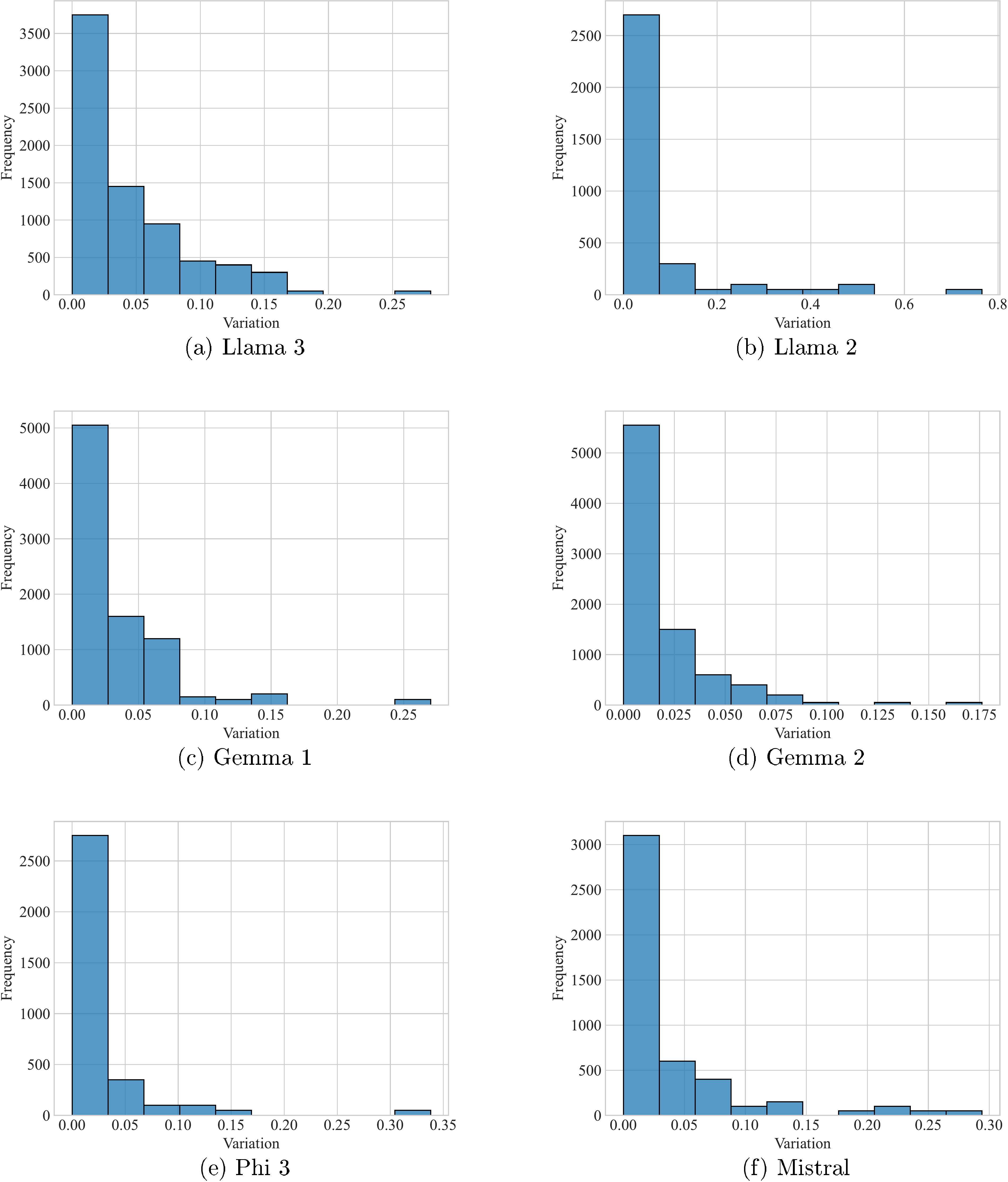
We also study whether the intermediate embeddings have outputs that are significantly different from those of the embedding extremes. In theory, we would expect the probability of an output computed on an intermediate embedding to be an interpolation between the value for one object or the other. Let

f (a)

be the probability score for one extreme of the interpolation and

f (b)

the probability score for the other extreme. We consider our expected range as

[min⁡(f(a),f(b)),max⁡(f(a),f(b))][\min(f(a), f(b)), \max(f(a), f(b))]

. We then verify whether, for some intermediate value, the predicted probability of 'yes' or 'no' is outside their respective ranges.⁶ In particular, we compute the maximum difference between the allowed range and the actual value, i.e.:

Note that increasing the probability of 'yes' does not necessarily decrease the probability of 'no', as the model can also provide spurious outputs.

\tag{24}

We define

mmaxm_{\text{max}}

as the maximum of the

mdiffm_{\text{diff}}

values for 'yes' and 'no'. Note that if the function only has values in

[min⁡(f(a),f(b)),max⁡(f(a),f(b))][\min(f(a), f(b)), \max(f(a), f(b))]

mmaxm_{\text{max}}

will be 0. We report the average

mmaxm_{\text{max}}

and the percentage of records where

mmax≥0.05m_{\text{max}} \geq 0.05

in Table 10. We also report the histograms describing the distributions of

mmaxm_{\text{max}}

in Figure 28. In general, we observe on average that 20% of records have an

mmaxm_{\text{max}}

higher than 0.05, which cannot be explained by a simple interpolation-based model of LLM behaviour.

Table 10: Average $m_{\text{max}}$ for each model and percentage of records where $m_{\text{max}} > 0.05$ . The "global" row is an average weighted by the number of valid records.

Model Name	Average $m_{\text{max}}$	% ( $m_{\text{max}} \geq 0.05$ )
Llama 3 8b	0.0434	32.43%
Llama 2 13b	0.0639	23.53%
Gemma 1 7b	0.0332	22.02%
Gemma 2 9b	0.0178	9.52%

D. Additional Results

Show me a brief summary.

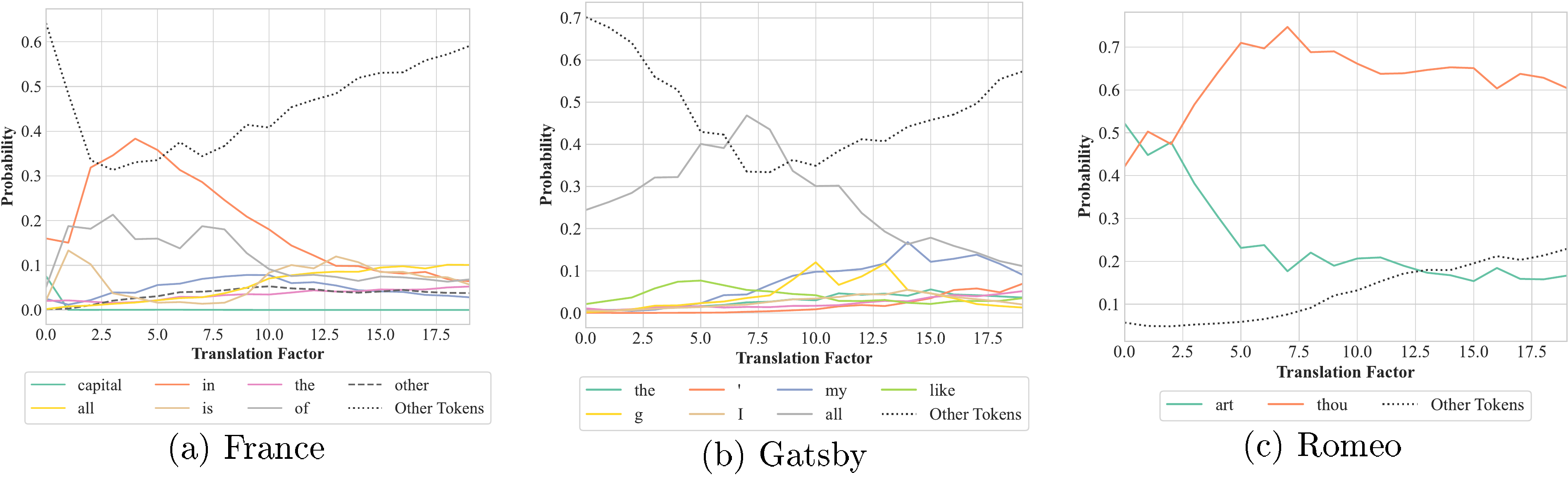
In this section, the authors investigate how large language models respond to two fundamental sequence transformations—shifting and scaling—to better understand temporal continuity in Transformers. They increment positional embeddings by fixed amounts (translation) and uniformly scale sentence durations across multiple models and sentences including "The capital of France is," "The Great Gatsby is my favourite," and "O Romeo, Romeo, wherefore art thou." The experiments reveal that shifting produces negligible changes in model outputs, demonstrating translational invariance attributable to the robustness of positional and rotary embeddings to relative position preservation, whereas scaling significantly alters outputs, indicating that duration itself is an intrinsic property affecting interpretation. These findings hold across models with rotary positional encoding, and even GPT2 with learned positional embeddings exhibits translational invariance for moderate shifts, though less strongly. The results suggest that LLMs interpret time continuously and that duration-based interpolation may explain their robustness on rare training inputs through semantic embedding interpolation.

We complement our previous observations on time continuity with experiments on two common sequence transformations, namely shifting and scaling.

D.1 Translational Invariance

For shifting, we increment the positional embeddings of each token (as well as the lower bound of integration) by a fixed amount (up to 10) without actually changing the sentence's duration. In particular, we feed the following input to Llama3-8B:

\quad

$\underbrace{\texttt{The}}_\xrightarrow{\Delta d} d_{s_1}$ $\underbrace{\texttt{capital}}_\xrightarrow{\Delta d} d_{s_2}$ $\underbrace{\texttt{of}}_\xrightarrow{\Delta d} d_{s_3}$ $\underbrace{\texttt{France}}_\xrightarrow{\Delta d} d_{s_4}$ $\underbrace{\texttt{is}}_\xrightarrow{\Delta d} d_{s_5}$

In addition to the sentence "The capital of France is", we study the following sentences:

"The Great Gatsby is my favourite";
"O Romeo, Romeo, wherefore art thou".

We report our full results for translation in Figures 41 to 43.

D.2 (Lack of) Scale Invariance

On the other hand, for scaling we increase/decrease the duration of the entire sentence:

$\underbrace{\texttt{\scalebox{1.5}[0.8]{The}}}_d_{s_1} > 1$ $\underbrace{\texttt{\scalebox{1.5}[0.8]{capital}}}_d_{s_2} > 1$ $\underbrace{\texttt{\scalebox{1.5}[0.8]{of}}}_d_{s_3} > 1$ $\underbrace{\texttt{\scalebox{1.5}[0.8]{France}}}_d_{s_4} > 1$ $\underbrace{\texttt{\scalebox{1.5}[0.8]{is}}}_d_{s_5} > 1$

See Figures 44 to 46 for our results.

D.3 Analysis

As shown for instance in Figure 47, we find that while the impact of shifting on an LLM's output is negligible, scaling significantly changes how the LLM interprets the input (and thus what the LLM outputs). This phenomenon occurs regardless of the model and sentence, empirically confirming the theoretical observations we already made about translation invariance in Section 3.

We believe that shifting does not affect an LLM's output due to the fact that positional and rotary-embeddings [20, 23] are robust to translations: as long as the relative positions between tokens are preserved, a model's output remains consistent. On the other hand, scaling leads to significant variations in an LLM's output.

Our results suggest that beyond interpreting time continuously, duration is itself an intrinsic property of our generalised Transformers that can explain why LLMs are robust on inputs with low frequency in the training data (e.g., their embedding may interpolate with others with similar semantics).

D.4 Shifting Invariance with Learned Positional Embeddings

While the properties of common positional encodings (in particular sinusoidal position encoding and Rotary Positional Encoding) inherently incentivise translation invariance, we study whether such a phenomenon takes place in models with learned positional encodings. To do so, we repeat our experiments with translation in GPT2, which uses this form of encoding.

We report our results in Figure 48. While the magnitude of the effect is certainly less strong compared to RoPE encodings, we observe that the top class remains consistent under translation for moderate shifts, which is consistent with our RoPE results.

References

Show me a brief summary.

In this section, the references span foundational and contemporary work across linguistics, natural language processing, and machine learning, establishing the theoretical and empirical context for continuous interpretations of language models. The citations trace the evolution from discrete linguistic theories and early statistical language models through neural probabilistic approaches, word embeddings, and recurrent architectures to modern transformer-based large language models including GPT, BERT, LLaMA, Mistral, and Gemma families. Key themes include positional encodings, attention mechanisms, and training paradigms like reinforcement learning from human feedback. The references also cover emerging continuous-time formulations, including neural ordinary differential equations applied to transformers, diffusion-based language models, and continuous space representations. Additionally, they address interpretability research on geometric properties of embeddings, linear representations, and feature extraction in LLMs. Together, these works underpin the paper's exploration of treating language models as continuous dynamical systems rather than purely discrete token processors, revealing novel insights into model behavior under interpolation and transformation.

[1] Charles F Hockett and Charles D Hockett. The origin of speech. Scientific American, 203(3):88–97, 1960.

[2] Noam Chomsky. Language and nature. Mind, 104(413):1–61, 1995.

[3] Michael Studdert-Kennedy. How did language go discrete. Language origins: Perspectives on evolution, ed. M. Tallerman, pp. 48–67, 2005.

[4] Adrian Akmajian, Ann K Farmer, Lee Bickmore, Richard A Demers, and Robert M Harnish. Linguistics: An introduction to language and communication. MIT press, 2017.

[5] Christopher D Manning. Foundations of statistical natural language processing. The MIT Press, 1999.

[6] Yoshua Bengio, Réjean Ducharme, and Pascal Vincent. A neural probabilistic language model. Advances in neural information processing systems, 13, 2000.

[7] Andriy Mnih and Geoffrey E Hinton. A scalable hierarchical distributed language model. Advances in neural information processing systems, 21, 2008.

[8] Jacob Devlin. Bert: Pre-training of deep bidirectional transformers for language understanding. arXiv preprint arXiv:1810.04805, 2018.

[9] Tom B. Brown, Benjamin Mann, Nick Ryder, et al. Language models are few-shot learners. In Advances in Neural Information Processing Systems 33: Annual Conference on Neural Information Processing Systems 2020, NeurIPS 2020, December 6-12, 2020, virtual, 2020. URL https://proceedings.neurips.cc/paper/2020/hash/1457c0d6bfcb4967418bfb8ac142f64a-Abstract.html.

[10] Matthew E. Peters, Mark Neumann, Mohit Iyyer, Matt Gardner, Christopher Clark, Kenton Lee, and Luke Zettlemoyer. Deep contextualized word representations. In Marilyn Walker, Heng Ji, and Amanda Stent (eds.), Proceedings of the 2018 Conference of the North American Chapter of the Association for Computational Linguistics: Human Language Technologies, Volume 1 (Long Papers), pp. 2227–2237, New Orleans, Louisiana, June 2018. Association for Computational Linguistics. doi:10.18653/v1/N18-1202. URL https://aclanthology.org/N18-1202.

[11] Alec Radford, Jeffrey Wu, Rewon Child, David Luan, Dario Amodei, Ilya Sutskever, et al. Language models are unsupervised multitask learners. OpenAI blog, 1(8):9, 2019.

[12] John Schulman, Filip Wolski, Prafulla Dhariwal, Alec Radford, and Oleg Klimov. Proximal policy optimization algorithms. arXiv preprint arXiv:1707.06347, 2017.

[13] Rafael Rafailov, Archit Sharma, Eric Mitchell, Christopher D Manning, Stefano Ermon, and Chelsea Finn. Direct preference optimization: Your language model is secretly a reward model. Advances in Neural Information Processing Systems, 36, 2024.

[14] Tamer Alkhouli, Andreas Guta, and Hermann Ney. Vector space models for phrase-based machine translation. In Dekai Wu, Marine Carpuat, Xavier Carreras, and Eva Maria Vecchi (eds.), Proceedings of SSST-8, Eighth Workshop on Syntax, Semantics and Structure in Statistical Translation, pp. 1–10, Doha, Qatar, October 2014. Association for Computational Linguistics. doi:10.3115/v1/W14-4001. URL https://aclanthology.org/W14-4001.

[15] Samuel R Bowman, Luke Vilnis, Oriol Vinyals, Andrew M Dai, Rafal Jozefowicz, and Samy Bengio. Generating sentences from a continuous space. arXiv preprint arXiv:1511.06349, 2015.

[16] Raffaele Guarasci, Giuseppe De Pietro, and Massimo Esposito. Quantum natural language processing: Challenges and opportunities. Applied sciences, 12(11):5651, 2022.

[17] Tomas Mikolov, Ilya Sutskever, Kai Chen, Greg S Corrado, and Jeff Dean. Distributed representations of words and phrases and their compositionality. Advances in neural information processing systems, 26, 2013a.

[18] S Hochreiter. Long short-term memory. Neural Computation MIT-Press, 1997.

[19] Martin Sundermeyer, Ralf Schlüter, and Hermann Ney. Lstm neural networks for language modeling. In Interspeech, volume 2012, pp. 194–197, 2012.

[20] Ashish Vaswani, Noam Shazeer, Niki Parmar, Jakob Uszkoreit, Llion Jones, Aidan N. Gomez, Lukasz Kaiser, and Illia Polosukhin. Attention is all you need. In Advances in Neural Information Processing Systems 30: 2017, December 4-9, 2017, Long Beach, CA, USA, pp. 5998–6008, 2017. URL https://proceedings.neurips.cc/paper/2017/hash/3f5ee243547dee91fbd053c1c4a845aa-Abstract.html.

[21] Abhimanyu Dubey, Abhinav Jauhri, Abhinav Pandey, Abhishek Kadian, Ahmad Al-Dahle, Aiesha Letman, Akhil Mathur, Alan Schelten, Amy Yang, Angela Fan, et al. The llama 3 herd of models. arXiv preprint arXiv:2407.21783, 2024.

[22] Albert Q Jiang, Alexandre Sablayrolles, Arthur Mensch, Chris Bamford, Devendra Singh Chaplot, Diego de las Casas, Florian Bressand, Gianna Lengyel, Guillaume Lample, Lucile Saulnier, et al. Mistral 7b. arXiv preprint arXiv:2310.06825, 2023.

[23] Gemma Team, Morgane Riviere, Shreya Pathak, Pier Giuseppe Sessa, Cassidy Hardin, Surya Bhupatiraju, Léonard Hussenot, Thomas Mesnard, Bobak Shahriari, Alexandre Ramé, et al. Gemma 2: Improving open language models at a practical size. arXiv preprint arXiv:2408.00118, 2024b.

[24] Antonio Fonseca, Emanuele Zappala, Josue Ortega Caro, and David van Dijk. Continuous spatiotemporal transformers, 2023. URL https://arxiv.org/abs/2301.13338.

[25] Ricky T. Q. Chen, Yulia Rubanova, Jesse Bettencourt, and David Duvenaud. Neural ordinary differential equations, 2019. URL https://arxiv.org/abs/1806.07366.

[26] Patrick Kidger. On neural differential equations, 2022. URL https://arxiv.org/abs/2202.02435.

[27] Yuqi Chen, Kan Ren, Yansen Wang, Yuchen Fang, Weiwei Sun, and Dongsheng Li. Contiformer: Continuous-time transformer for irregular time series modeling. Advances in Neural Information Processing Systems, 36, 2024.

[28] Fernando Moreno-Pino, Álvaro Arroyo, Harrison Waldon, Xiaowen Dong, and Álvaro Cartea. Rough transformers: Lightweight continuous-time sequence modelling with path signatures, 2024. URL https://arxiv.org/abs/2405.20799.

[29] Patrick Kidger, James Morrill, James Foster, and Terry Lyons. Neural controlled differential equations for irregular time series. In H. Larochelle, M. Ranzato, R. Hadsell, M.F. Balcan, and H. Lin (eds.), Advances in Neural Information Processing Systems, volume 33, pp. 6696–6707. Curran Associates, Inc., 2020. URL https://proceedings.neurips.cc/paper_files/paper/2020/file/4a5876b450b45371f6cfe5047ac8cd45-Paper.pdf.

[30] James Morrill, Cristopher Salvi, Patrick Kidger, and James Foster. Neural rough differential equations for long time series. In Marina Meila and Tong Zhang (eds.), Proceedings of the 38th International Conference on Machine Learning, volume 139 of Proceedings of Machine Learning Research, pp. 7829–7838. PMLR, 18–24 Jul 2021. URL https://proceedings.mlr.press/v139/morrill21b.html.

[31] Bei Li, Quan Du, Tao Zhou, Yi Jing, Shuhan Zhou, Xin Zeng, Tong Xiao, JingBo Zhu, Xuebo Liu, and Min Zhang. ODE transformer: An ordinary differential equation-inspired model for sequence generation. In Smaranda Muresan, Preslav Nakov, and Aline Villavicencio (eds.), Proceedings of the 60th Annual Meeting of the Association for Computational Linguistics (Volume 1: Long Papers), pp. 8335–8351, Dublin, Ireland, May 2022a. Association for Computational Linguistics. doi:10.18653/v1/2022.acl-long.571. URL https://aclanthology.org/2022.acl-long.571.

[32] Jing Zhang, Peng Zhang, Baiwen Kong, Junqiu Wei, and Xin Jiang. Continuous self-attention models with neural ode networks. In Proceedings of the AAAI Conference on Artificial Intelligence, volume 35, pp. 14393–14401, 2021.

[33] Subhabrata Dutta, Tanya Gautam, Soumen Chakrabarti, and Tanmoy Chakraborty. Redesigning the transformer architecture with insights from multi-particle dynamical systems. Advances in Neural Information Processing Systems, 34:5531–5544, 2021.

[34] Aaron Baier-Reinio and Hans De Sterck. N-ode transformer: A depth-adaptive variant of the transformer using neural ordinary differential equations. arXiv preprint arXiv:2010.11358, 2020.

[35] Zineng Tang, Shiyue Zhang, Hyounghun Kim, and Mohit Bansal. Continuous language generative flow. In Chengqing Zong, Fei Xia, Wenjie Li, and Roberto Navigli (eds.), Proceedings of the 59th Annual Meeting of the Association for Computational Linguistics and the 11th International Joint Conference on Natural Language Processing (Volume 1: Long Papers), pp. 4609–4622, Online, August 2021. Association for Computational Linguistics. doi:10.18653/v1/2021.acl-long.355. URL https://aclanthology.org/2021.acl-long.355.

[36] Holger Schwenk. Continuous space language models. Computer Speech & Language, 21(3):492–518, 2007. ISSN 0885-2308. doi:https://doi.org/10.1016/j.csl.2006.09.003. URL https://www.sciencedirect.com/science/article/pii/S0885230806000325.

[37] Robert Östling and Jörg Tiedemann. Continuous multilinguality with language vectors. In Mirella Lapata, Phil Blunsom, and Alexander Koller (eds.), Proceedings of the 15th Conference of the European Chapter of the Association for Computational Linguistics: Volume 2, Short Papers, pp. 644–649, Valencia, Spain, April 2017. Association for Computational Linguistics. URL https://aclanthology.org/E17-2102.

[38] Xiang Li, John Thickstun, Ishaan Gulrajani, Percy S Liang, and Tatsunori B Hashimoto. Diffusion-lm improves controllable text generation. Advances in Neural Information Processing Systems, 35:4328–4343, 2022b.

[39] Shansan Gong, Mukai Li, Jiangtao Feng, Zhiyong Wu, and LingPeng Kong. Diffuseq: Sequence to sequence text generation with diffusion models. arXiv preprint arXiv:2210.08933, 2022.

[40] Justin Lovelace, Varsha Kishore, Yiwei Chen, and Kilian Q Weinberger. Diffusion guided language modeling. arXiv preprint arXiv:2408.04220, 2024a.

[41] Ishaan Gulrajani and Tatsunori B Hashimoto. Likelihood-based diffusion language models. Advances in Neural Information Processing Systems, 36, 2024.

[42] Yizhe Zhang, Jiatao Gu, Zhuofeng Wu, Shuangfei Zhai, Joshua Susskind, and Navdeep Jaitly. Planner: generating diversified paragraph via latent language diffusion model. Advances in Neural Information Processing Systems, 36, 2024.

[43] Justin Lovelace, Varsha Kishore, Chao Wan, Eliot Shekhtman, and Kilian Q Weinberger. Latent diffusion for language generation. Advances in Neural Information Processing Systems, 36, 2024b.

[44] Wes Gurnee and Max Tegmark. Language models represent space and time. arXiv preprint arXiv:2310.02207, 2023.

[45] Andy Arditi, Oscar Obeso, Aaquib Syed, Daniel Paleka, Nina Panickssery, Wes Gurnee, and Neel Nanda. Refusal in language models is mediated by a single direction. arXiv preprint arXiv:2406.11717, 2024.

[46] Anthropic. Scaling monosemanticity: Extracting interpretable features from claude 3 sonnet. Transformer Circuits, 2024. URL https://transformer-circuits.pub/2024/scaling-monosemanticity/index.html.

[47] Shauli Ravfogel, Michael Twiton, Yoav Goldberg, and Ryan D Cotterell. Linear adversarial concept erasure. In International Conference on Machine Learning, pp. 18400–18421. PMLR, 2022.

[48] Eric Todd, Millicent L Li, Arnab Sen Sharma, Aaron Mueller, Byron C Wallace, and David Bau. Function vectors in large language models. arXiv preprint arXiv:2310.15213, 2023.

[49] Luke Vilnis and Andrew McCallum. Word representations via gaussian embedding. arXiv preprint arXiv:1412.6623, 2014.

[50] Ryan Cotterell, Anej Svete, Clara Meister, Tianyu Liu, and Li Du. Formal aspects of language modeling. arXiv preprint arXiv:2311.04329, 2023.

[51] Hugo Touvron, Louis Martin, Kevin Stone, Peter Albert, Amjad Almahairi, Yasmine Babaei, Nikolay Bashlykov, Soumya Batra, Prajjwal Bhargava, Shruti Bhosale, et al. Llama 2: Open foundation and fine-tuned chat models. arXiv preprint arXiv:2307.09288, 2023.

[52] Marah Abdin, Sam Ade Jacobs, Ammar Ahmad Awan, Jyoti Aneja, Ahmed Awadallah, Hany Awadalla, Nguyen Bach, Amit Bahree, Arash Bakhtiari, Harkirat Behl, et al. Phi-3 technical report: A highly capable language model locally on your phone. arXiv preprint arXiv:2404.14219, 2024.

[53] Gemma Team, Thomas Mesnard, Cassidy Hardin, Robert Dadashi, Surya Bhupatiraju, Shreya Pathak, Laurent Sifre, Morgane Rivière, Mihir Sanjay Kale, Juliette Love, et al. Gemma: Open models based on gemini research and technology. arXiv preprint arXiv:2403.08295, 2024a.

[54] Tomas Mikolov, Wen-tau Yih, and Geoffrey Zweig. Linguistic regularities in continuous space word representations. In Lucy Vanderwende, Hal Daumé III, and Katrin Kirchhoff (eds.), Proceedings of the 2013 Conference of the North American Chapter of the Association for Computational Linguistics: Human Language Technologies, pp. 746–751, Atlanta, Georgia, June 2013b. Association for Computational Linguistics. URL https://aclanthology.org/N13-1090.

[55] Kiho Park, Yo Joong Choe, and Victor Veitch. The linear representation hypothesis and the geometry of large language models. arXiv preprint arXiv:2311.03658, 2023.

[56] Fangru Lin, Emanuele La Malfa, Valentin Hofmann, Elle Michelle Yang, Anthony Cohn, and Janet B Pierrehumbert. Graph-enhanced large language models in asynchronous plan reasoning. arXiv preprint arXiv:2402.02805, 2024.

Model Name	Valid Ratio
Llama 3 8b	93.5%
Llama 2 13b	54.5%
Gemma 1 7b	100.0%
Gemma 2 9b	100.0%

Model Name	Valid Rate
Llama 3 8b	60.0%
Llama 2 13b	19.5%
Gemma 1 7b	94.5%
Gemma 2 9b	95.0%

Model Name	Normalised Maximum Absolute Derivative
Llama 3 8b	4.959
Llama 2 13b	9.005
Gemma 1 7b	5.090
Gemma 2 9b	5.402