KronQ: LLM Quantization via Kronecker-Factored Hessian

Donghyun Lee $^{1}$, Yuhang Li $^{2}$, Ruokai Yin $^{2}$, Priyadarshini Panda $^{1}$ $^{1}$ University of Southern California, $^{2}$ Yale University [email protected] centerlineGitHub https://github.com/Intelligent-Computing-Lab-Panda/KronQ

Abstract

Post-training quantization (PTQ) is a widely adopted technique for compressing large language models (LLMs) without retraining. Existing second-order PTQ methods, including GPTQ, construct quantization objectives exclusively from input activation statistics, effectively assuming that all output channels contribute equally to the layer-wise reconstruction objective. We propose $\textsc{KronQ}$, a PTQ framework that challenges this assumption by introducing the gradient covariance into the quantization pipeline. Under the Kronecker-factored Hessian approximation, the quantization loss depends jointly on both the activation and gradient covariances, and $\textsc{KronQ}$ exploits this at two complementary levels. (1) $\textsc{KronQ}$ introduces bidirectional incoherence processing, extending the existing input-side random rotation to the output dimension using the gradient covariance, reducing weight magnitude variance across both input and output dimensions. (2) $\textsc{KronQ}$ derives a new sensitivity metric for inter-layer mixed-precision allocation, driven by the gradient and activation Hessian traces. Notably, in the case of 2-bit weight-only quantization on LLaMA-3-70B, while GPTQ and GPTAQ diverge or produce degenerate quantizations (

gt;$2000 perplexity on WikiText-2), $\textsc{KronQ}$ achieves 7.93 perplexity.

Executive Summary: KronQ is a new post-training quantization technique for large language models that incorporates both input activation statistics and output gradient statistics to compress weights more accurately. Existing methods such as GPTQ rely solely on input activation covariances and treat all output channels as equally important. This assumption breaks down at very low bit widths, where models like LLaMA-3-70B produce unusable outputs or diverge entirely.

The work set out to test whether adding gradient covariance information, obtained from a single backward pass, could improve quantization quality without changing the core solver or adding runtime cost. The approach applies the Kronecker-factored Hessian approximation to derive a joint objective over input and output factors, then introduces bidirectional incoherence processing (random orthogonal transforms on both dimensions) and a new mixed-precision sensitivity score based on the product of the two Hessian traces. Experiments covered LLaMA-2 and LLaMA-3 models from 7B to 70B parameters, weight-only and weight-and-activation settings at 2-, 3-, and 4-bit, plus newer families such as Gemma-3 and DeepSeek-R1, all calibrated on 128 WikiText-2 sequences.

At 2-bit weight-only quantization on LLaMA-3-70B, GPTQ and GPTAQ either diverge or exceed 2000 perplexity while KronQ reaches 7.93. Gains are largest in the 2-bit regime across all tested models and remain consistent at higher bits. The mixed-precision allocation using the joint trace score yields better perplexity at the same average bit width than activation-only ranking. Memory footprint drops by 3.5–7.5× and decoding speed improves by 1.25–2.51× relative to the unquantized baseline. The same pattern holds on reasoning benchmarks and generative tasks, where KronQ roughly doubles accuracy over GPTAQ in several cases.

These results matter because reliable 2-bit and 3-bit quantization directly reduces the hardware needed to serve frontier models. A 70B model that requires two A100 GPUs in 16-bit fits on one GPU at 4-bit, lowering both capital and energy costs and enabling deployment on edge or single-GPU servers. The method preserves the practical one-shot workflow already used in production libraries, so integration cost is low.

Organizations running large-scale inference should evaluate KronQ in their quantization pipelines, starting with weight-only 2-bit and 3-bit settings where the margin over prior methods is greatest. Mixed-precision allocation can be applied selectively on the most sensitive sublayers to meet a target average bit width. Further work should focus on reducing the one-time backward-pass cost for gradient covariance estimation and on testing a broader set of architectures. The main limitations are the modest extra offline memory during preprocessing and the small online rotation overhead at inference, both of which are already comparable to existing rotation-based methods. Results are reproducible on the reported models and calibration regime with high confidence.

1. Introduction

Section Summary: Large language models have grown so large that running them on ordinary hardware requires heavy compression, and one practical approach called post-training quantization reduces weights to low-precision numbers using only a small calibration set without any retraining. Current leading methods improve accuracy by compensating for quantization errors with input activation statistics, yet they ignore important information about how much each output direction affects the model, which leads to suboptimal results especially at very low bit widths. The paper introduces KronQ, which incorporates both input and output gradient information through a Kronecker-factored approximation of the full Hessian and adds mixed-precision allocation across layers, delivering consistent accuracy gains on LLaMA models from 7B to 70B parameters.

Large language models (LLMs) have achieved remarkable performance across a wide range of natural language understanding and generation tasks ([1, 2, 3]). However, their growing parameter counts, reaching hundreds of billions in recent models, pose significant deployment challenges, as the memory and computational requirements far exceed what is available on commodity and edge hardware. Quantization ([4, 5]) provides an effective solution by compressing model weights and activations to low-bit representations, reducing both memory footprint and inference latency. Among quantization techniques, post-training quantization (PTQ) has attracted particular interest due to its practicality. It requires no retraining and operates on a pretrained model using only a small calibration dataset.

PTQ methods for LLMs span several paradigms ([6]): (1) Compensation-based methods apply the Optimal Brain Surgeon (OBS) principle ([7, 8]) layer-by-layer, using the input activation covariance as a proxy Hessian to compensate for rounding error in weight quantization ([9, 10, 11, 12, 13, 14]). (2) Rotation-based methods apply orthogonal transforms to weight matrices and activations to suppress outliers before quantization ([15, 16, 17, 18]). (3) Salience-based methods identify sensitive weight channels via activation magnitudes and protect them through per-channel scaling ([19, 20]). These paradigms are complementary and are often combined in practice. In this work, we focus on the compensation-based family, in particular GPTQ ([10]) and its successors, combined with orthogonal transforms from the rotation-based paradigm. These methods have become the dominant framework for LLM weight quantization and are widely integrated into production serving stacks, including HuggingFace Transformers ([21]), GPTQModel ([22]), and vLLM ([23]).

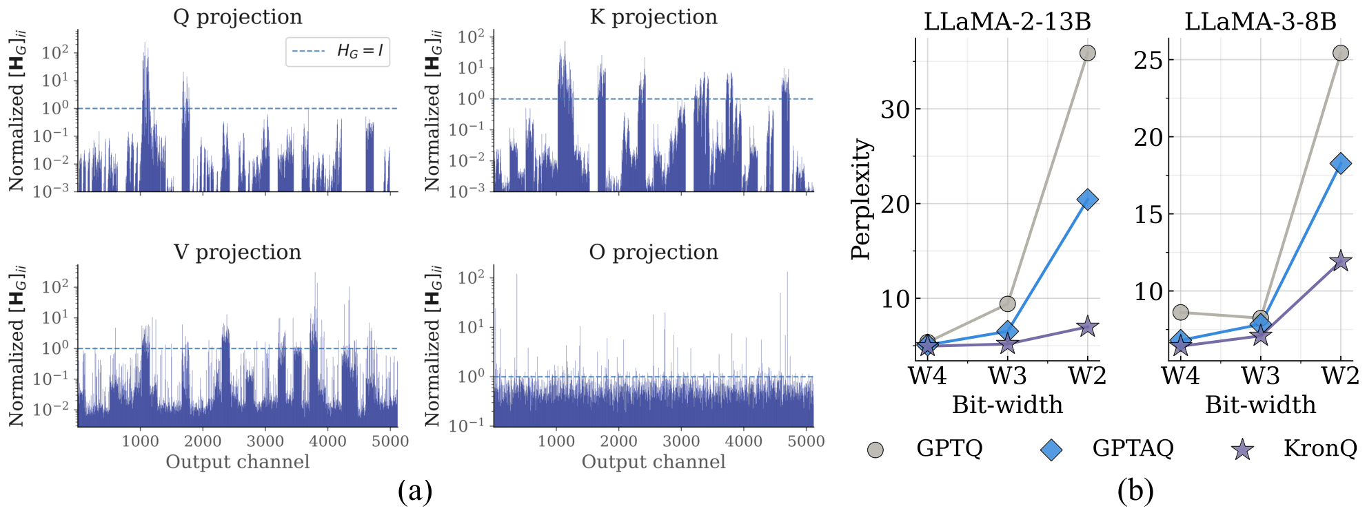
However, compensation-based methods share a fundamental limitation: the quantization objective is characterized solely through the input activation covariance $\mathbf{H}_X$, which captures only the input-side second-order information of the weight space. Under the Kronecker-factored approximation (K-FAC) ([24]), the full weight Hessian factorizes as $\mathbf{H} \approx \mathbf{H}_X \otimes \mathbf{H}_G$, where $\mathbf{H}_G = \mathbb{E}[\mathbf{gg}^\top]$ is the gradient covariance with $g$ as the output gradient. Yet compensation-based methods built on the GPTQ-style ([10]) column-wise OBS solver leave $\mathbf{H}_G$ unused, implicitly treating all output directions as equally important by assuming $\mathbf{H}_G = \mathbf{I}$. As shown in Figure 1(a), output channels vary substantially in gradient magnitude, making this a suboptimal approximation.

We propose $\textsc{KronQ}$, a post-training quantization method built on the Kronecker-factored Hessian approximation $\mathbf{H} \approx \mathbf{H}_X \otimes \mathbf{H}_G$. By incorporating the gradient covariance $\mathbf{H}_G$ into the quantization objective, $\textsc{KronQ}$ accounts for output-side Hessian information, a dimension entirely overlooked by existing compensation-based methods. Our contributions are as follows.

1. Kronecker-Factored Quantization Error. We extend the layer-wise quantization objective to incorporate $\mathbf{H}_G$ under the K-FAC approximation and introduce bidirectional incoherence processing. Notably, $\mathbf{H}_G$ cancels in the quantization update, preserving the efficiency of the base quantizer.
2. Inter-Layer Mixed Precision via Joint Hessian Traces. We derive a sublayer sensitivity metric from $\mathrm{tr}(\mathbf{H}_G) \cdot \mathrm{tr}(\mathbf{H}_X)$ that differentiates sublayers sharing identical input statistics, enabling optimal bit-width allocation across sublayers.
3. Empirical Validation. We evaluate $\textsc{KronQ}$ on LLaMA-2 and LLaMA-3 from 7B to 70B across weight-only and weight-and-activation settings at W2/W3/W4, achieving consistent state-of-the-art results with the largest gains at 2-bit, as shown in Figure 1(b).

2. Related Work

Section Summary: Recent research on post-training quantization for large language models falls into three main categories. Compensation-based techniques, building on the Optimal Brain Surgeon framework, use input statistics and Hessian approximations to adjust weights during quantization, with later refinements that correct for error accumulation or add output-aware information. Rotation-based methods apply special transformations to reduce outlier values and enable lower-bit representations, while mixed-precision approaches assign varying bit widths to different layers or weights, often guided by importance scores derived from activation or gradient data.

Compensation-Based Post-Training Quantization.

The Optimal Brain Surgeon (OBS) framework ([7, 8]) provides the theoretical basis for Hessian-guided weight perturbation. GPTQ ([10]) scales this to LLMs by performing column-wise OBS updates using the input activation covariance $\mathbf{H}_X$ as a proxy Hessian, establishing the de facto standard for one-shot LLM quantization. BoA ([11]) extends GPTQ with attention-aware Hessians that capture inter-layer interactions within the attention module. GPTAQ ([12]) improves upon GPTQ by correcting for input drift caused by prior-layer quantization errors that accumulate during sequential layer-wise quantization, substantially reducing perplexity at ultra-low bit-widths. Two recent methods go beyond input-only statistics. GuidedQuant ([14]) reweights $\mathbf{H}_X$ with end-loss gradient saliency but ignores cross-output-channel structure. YAQA ([13]), the most closely related to our work, adopts the same factorization $\mathbf{H} \approx \mathbf{H}_X \otimes \mathbf{H}_G$ but folds $\mathbf{H}_G$ into a modified LDLQ solver via costly power-iterated Hessian sketches. In contrast, KronQ obtains $\mathbf{H}_G$ from a single backward pass and keeps the solver exactly GPTAQ, using $\mathbf{H}_G$ only for incoherence processing and mixed-precision allocation.

Rotation-Based Post-Training Quantization.

QuaRot ([17]) and SpinQuant ([18]) apply orthogonal transforms to weight matrices and activations to suppress outliers, enabling low-bit weight-and-activation quantization. QuIP ([15]) establishes the theoretical foundation, showing that incoherent weight and Hessian matrices yield lower quantization error, and QuIP# ([16]) extends this with the randomized Hadamard transform and lattice-based vector quantization for practical 2-bit quantization. More recent methods explore learnable transformations, including Kronecker-structured affine maps ([25]) and jointly optimized orthogonal and scaling transforms ([26]).

Mixed-Precision Quantization. Mixed-precision methods differ in granularity. Intra-layer methods allocate bit-widths within a layer: SliM-LLM ([27]) uses weight saliency and CMPQ ([28]) uses activation norms. Inter-layer methods assign one bit-width per sublayer: HAWQ-V2 ([29]) ranks layers by Hessian traces, while AMQ ([30]), Q-Palette ([31]), and HIGGS ([32]) rely on evolutionary search, dynamic programming, and a linearity theorem, respectively. All use only $\mathbf{H}_X$, which is shared across Q, K, V and cannot differentiate them, whereas the KronQ score $\mathrm{tr}(\mathbf{H}_G)\cdot\mathrm{tr}(\mathbf{H}_X)$ breaks this degeneracy via the output-side factor at the cost of a single backward pass.

3. Preliminary

Section Summary: The preliminary section reviews two families of techniques for reducing error when quantizing neural-network weights after training. Compensation-based methods such as GPTQ and its extension GPTAQ minimize the mismatch between a layer’s original and quantized outputs on calibration data; they do so by updating unquantized weights after each column is rounded and, in the case of GPTAQ, by additionally correcting for the drift in activations that occurs when earlier layers have already been quantized. Incoherence processing, used by QuIP and QuIP#, multiplies the weight matrix and its input-side sensitivity matrix by random orthogonal transformations so that large values are spread more uniformly, thereby tightening worst-case rounding error; however, both families of methods rely on sensitivity information derived only from the inputs and leave output-side gradient statistics unaccounted for.

3.1 Compensation-based Quantization

Let $\mathbf{X} \in \mathbb{R}^{d_{\mathrm{in}} \times n}$ be a matrix of $n$ calibration inputs stacked as columns, $\mathbf{W} \in \mathbb{R}^{d_{\mathrm{out}} \times d_{\mathrm{in}}}$ the weight matrix of a linear layer with input dimension $d_{\mathrm{in}}$ and output dimension $d_{\mathrm{out}}$, and $\widehat{\mathbf{W}}$ its quantized counterpart. The standard layer-wise PTQ objective minimizes the squared output reconstruction error:

$ \min_{\widehat{\mathbf{W}}} ; |\mathbf{W}\mathbf{X} - \widehat{\mathbf{W}}\mathbf{X}|_F^2 ;=; \mathrm{tr}!\left[(\mathbf{W} - \widehat{\mathbf{W}}), \mathbf{H}_X, (\mathbf{W} - \widehat{\mathbf{W}})^\top\right],\tag{1} $

where $\mathbf{H}X = \mathbf{X}\mathbf{X}^\top \in \mathbb{R}^{d{\mathrm{in}} \times d_{\mathrm{in}}}$ is the input activation covariance, which serves as a proxy for the layer-wise Hessian. GPTQ ([10]) solves this objective greedily column by column using the OBS ([7]) update. The compensation applied to the remaining unquantized columns after quantizing column $p$ is given by

$ \Delta\mathbf{W}{:, p+1:} = -\frac{\mathbf{W}{:, p} - \widehat{\mathbf{W}}_{:, p}}{[\mathbf{H}_X^{-1}] _{pp}} \cdot [\mathbf{H}_X^{-1}] _{p+1:, p},\tag{2} $

where $[\mathbf{H}_X^{-1}] _{pp}$ is the $p$-th diagonal entry of the inverse Hessian and $[\mathbf{H}_X^{-1}] {p+1:, p}$ is its $p$-th column restricted to rows $p+1$ onward. This distributes the quantization error of $\mathbf{W}{:, p}$ optimally to the remaining weights. However, the layer-wise framework causes quantization errors to accumulate across layers, as the objective in Equation 1 is evaluated on activations already degraded by prior-layer quantization. GPTAQ ([12]) addresses this by correcting for input drift via asymmetric calibration:

$ \min_{\widehat{\mathbf{W}}} ; |\mathbf{W}\widetilde{\mathbf{X}} - \widehat{\mathbf{W}}\mathbf{X}|F^2 ;=; \min{\widehat{\mathbf{W}}} \mathrm{tr}!\left[\Delta\mathbf{W}, \mathbf{H}_X, \Delta\mathbf{W}^\top

• \mathbf{W}, \Delta\mathbf{X}\mathbf{X}^\top, \Delta\mathbf{W}^\top \right],\tag{3} $

where $\Delta\mathbf{W} = \mathbf{W} - \widehat{\mathbf{W}}$, $\mathbf{X}$ is the input from the running quantized model, $\widetilde{\mathbf{X}}$ is the corresponding activation of the full-precision model, and $\Delta\mathbf{X} = \widetilde{\mathbf{X}} - \mathbf{X}$ is the input drift. Despite this correction, GPTAQ inherits the same proxy Hessian $\mathbf{H}_X$, leaving the output-side gradient statistics unaccounted for.

3.2 Incoherence Processing

Incoherence processing ([15]) is a preprocessing technique that reduces quantization error by spreading weight magnitudes uniformly across all dimensions. Formally, the incoherence of $\mathbf{W}$ and its proxy Hessian $\mathbf{H}_X$ are measured by

$ \mu(\mathbf{W}) = \frac{\sqrt{d_{\mathrm{out}} d_{\mathrm{in}}}}{|\mathbf{W}|F} \max{i, j} |\textbf{W}{ij}|, \qquad \mu(\mathbf{H}X) = \sqrt{d{\mathrm{in}}} \cdot \max{i, j} |\textbf{Q}_{ij}|,\tag{4} $

where $\mathbf{Q}$ denotes the eigenvector matrix of $\mathbf{H}X$, and lower $\mu$ leads to tighter quantization error bounds. Intuitively, this is achieved by randomizing the spectral directions of $\mathbf{W}$ and $\mathbf{H}X$, so that rounding sensitivity is no longer concentrated along specific coordinate axes. To this end, random orthogonal matrices $\mathbf{U} \in \mathbb{R}^{d{\mathrm{out}} \times d{\mathrm{out}}}$ and $\mathbf{V} \in \mathbb{R}^{d_{\mathrm{in}} \times d_{\mathrm{in}}}$ are applied:

$ \mathbf{W} \leftarrow \mathbf{U}\mathbf{W}\mathbf{V}^\top, \quad \mathbf{H}_X \leftarrow \mathbf{V} \mathbf{H}_X \mathbf{V}^\top.\tag{5} $

After quantization, the rotations must be applied online during inference. QuIP ([15]) instantiates $\mathbf{U}$ and $\mathbf{V}$ as Kronecker-structured random orthogonal matrices, introducing $\Theta(d_{\mathrm{in}}^{3/2} + d_{\mathrm{out}}^{3/2})$ inference overhead per layer. QuIP# ([16]) replaces these with randomized Hadamard transforms, reducing this to $\Theta(d_{\mathrm{in}} \log d_{\mathrm{in}} + d_{\mathrm{out}} \log d_{\mathrm{out}})$. However, this incoherence process accounts only for input-side Hessian information through $\mathbf{H}_X$, leaving the output-side entirely unaddressed.

4. Method

Section Summary: The method begins by replacing the standard post-training quantization loss with a Kronecker-factored approximation of the full layer Hessian, H_X ⊗ H_G, so that both input and output gradient statistics guide the rounding decisions; this leads to an efficient column-wise compensation rule that retains the H_G factor yet inherits the speed of prior GPTAQ-style updates. The authors then observe that the output-side factor H_G is highly coherent in practice, and therefore apply a novel row-wise diagonal rescaling (derived from H_G) together with the existing column-wise rescaling of H_X, producing a bidirectional incoherence transform that flattens weight magnitudes from both sides before quantization. Together these steps allow accurate low-bit compression while requiring only a single backward pass over calibration data.

4.1 Kronecker-Factored Quantization Error

The standard layer-wise PTQ objective in Equation 1 uses $\mathbf{H}_X$ as a proxy for the full Hessian $\mathbf{H}$, discarding the output-side statistics entirely. We recover this missing factor via the Kronecker-factored approximation ([24, 33]). For a linear layer $\mathbf{y} = \mathbf{W}\mathbf{x}$, the per-sample gradient factorizes as $\frac{\partial \mathcal{L}}{\partial \mathbf{W}} = \mathbf{g}\mathbf{x}^\top$, where $\mathbf{g} = \partial\mathcal{L}/\partial\mathbf{y}$. The empirical Fisher approximation of $\mathbf{H}$ ([34]) gives:

$ \begin{aligned} \mathbf{H} &;=; \mathbb{E}!\left[\mathrm{vec}!\left(\frac{\partial \mathcal{L}}{\partial \mathbf{W}}\right) \mathrm{vec}!\left(\frac{\partial \mathcal{L}}{\partial \mathbf{W}}\right)^\top \right] ;=; \mathbb{E}!\left[(\mathbf{x} \otimes \mathbf{g})(\mathbf{x} \otimes \mathbf{g})^\top \right] ;=; \mathbb{E}!\left[\mathbf{x}\mathbf{x}^\top \otimes \mathbf{g}\mathbf{g}^\top \right]. \end{aligned}\tag{6} $

Since the joint expectation $\mathbb{E}[\mathbf{x}\mathbf{x}^\top \otimes \mathbf{g}\mathbf{g}^\top] \in \mathbb{R}^{d_{\mathrm{out}}d_{\mathrm{in}} \times d_{\mathrm{out}}d_{\mathrm{in}}}$ is intractable, we apply the K-FAC independence assumption $\mathbf{x} \perp!!!\perp \mathbf{g}$ ([24, 35]), under which the expectation factorizes:

$ \mathbf{H} ;\approx; \mathbb{E}[\mathbf{x}\mathbf{x}^\top] \otimes \mathbb{E}[\mathbf{g}\mathbf{g}^\top] ;=:; \mathbf{H}_X \otimes \mathbf{H}_G,\tag{7} $

reducing complexity from $\mathcal{O}(d_{\mathrm{in}}^2 d_{\mathrm{out}}^2)$ to $\mathcal{O}(d_{\mathrm{in}}^2 + d_{\mathrm{out}}^2)$. Substituting Equation 7 into Equation 1 yields the Kronecker-factored quantization objective:

$ \min_{\widehat{\mathbf{W}}} ; \mathrm{tr}!\left[\mathbf{H}_G, \Delta\mathbf{W}, \mathbf{H}_X, \Delta\mathbf{W}^\top\right].\tag{8} $

Most existing PTQ methods implicitly set $\mathbf{H}G = \mathbf{I}$. However, as shown in Figure 1(a), output channels vary substantially in gradient magnitude, making this approximation suboptimal. $\textsc{KronQ}$ retains $\mathbf{H}G$, estimated via a single backward pass over the calibration set and stored as a $d{\mathrm{out}} \times d{\mathrm{out}}$ matrix. Building on GPTAQ ([12]), we further correct for input drift by incorporating the asymmetric correction from Equation 3:

$ \min_{\widehat{\mathbf{W}}} \mathrm{tr}!\left[\mathbf{H}_G!\left(\Delta\mathbf{W}, \mathbf{H}_X, \Delta\mathbf{W}^\top

• \mathbf{W}, \Delta\mathbf{X}\mathbf{X}^\top, \Delta\mathbf{W}^\top \right)\right].\tag{9} $

The optimal weight update under Equation 9 is characterized in the following proposition.

########## {caption="Proposition 1: KronQ Weight Compensation"}

Under the column-wise OBS update applied to 9, $\mathbf{H}_G$ cancels algebraically, and the weight compensation after quantizing column $p$ reduces to:

$ \Delta\mathbf{W}_{:, p+1:} = -\boldsymbol{\delta}_p, [\mathbf{H}_X^{-1}] _{p, p+1:}

• \mathbf{W}_{:, p} \cdot [\mathbf{P}] _{p, p+1:},\tag{10} $

where $\boldsymbol{\delta}p = (\mathbf{W}{:, p} - \widehat{\mathbf{W}}_{:, p})/[\mathbf{H}_X^{-1}] _{pp}$ is the scaled quantization error and $\mathbf{P} = \alpha, ((\Delta\mathbf{X}\mathbf{X}^\top \mathbf{H}_X^{-\top}) \cdot \mathrm{triu}), \mathbf{H}_X^{-1}$ is the GPTAQ asymmetric correction matrix.

The derivation of Proposition 1 is provided in Appendix A.1. $\textsc{KronQ}$ inherits the computational efficiency of GPTAQ while exploiting $\mathbf{H}_G$ for bidirectional incoherence processing and mixed-precision allocation.

4.2 Bidirectional Incoherence Processing

[15] and [16] show that quantization error can be reduced when the proxy Hessian is incoherent—its eigenvectors are not aligned with the coordinate axes—and that $\mathbf{H}_X$ is highly coherent in practice, motivating column-side incoherence processing. Under the $\textsc{KronQ}$ objective Equation 9, $\mathbf{H}_G$ appears as the complementary output-side Hessian factor. This raises a natural question: is $\mathbf{H}_G$ also coherent?

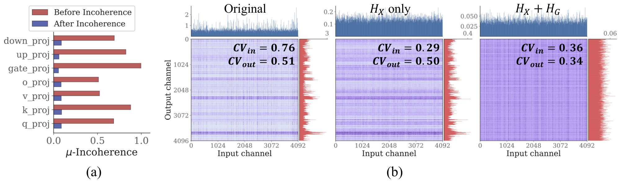
We answer this via the incoherence measure $\mu(\mathbf{H}G) = \sqrt{d{\mathrm{out}}} \cdot \max_{i, j} |\textbf{Q}{ij}|$ from Equation 4. Here, $\mu/\sqrt{d{\mathrm{out}}} \to 1$ indicates maximal coherence and $\mu/\sqrt{d_{\mathrm{out}}} \to 0$ indicates incoherence. Figure 2(a) presents $\mu(\mathbf{H}G)/\sqrt{d{\mathrm{out}}}$ before and after incoherence processing across sublayers of LLaMA-2-7B. $\mu(\mathbf{H}G)/\sqrt{d{\mathrm{out}}}$ reaches up to $0.99$, but it drops below $0.10$ for all sublayers after incoherence processing, confirming that output-side rotation effectively incoherences $\mathbf{H}_G$. This motivates bidirectional incoherence processing (BiIP). Extending the input-side diagonal rescaling of [15] to both column and row directions, we apply:

$ \mathbf{W} ;\leftarrow; \mathbf{S}_G, \mathbf{W}, \mathbf{S}_X, \qquad \mathbf{S}_X = \mathrm{diag}!\left(\frac{[\mathbf{H}_X] {jj}} {|\mathbf{W}{:, j}|^2}\right)^{1/4}!, \quad \mathbf{S}_G = \mathrm{diag}!\left(\frac{[\mathbf{H}_G] {ii}} {|\mathbf{W}{i, :}|^2}\right)^{1/4}!,\tag{11} $

where the output-side $\mathbf{S}_G$ term, derived from $\mathbf{H}_G$, is novel. Since the subsequent quantization operates in the rescaled weight space, the Hessians are transformed accordingly as $\mathbf{H}_X \leftarrow \mathbf{S}_X^{-1} \mathbf{H}_X \mathbf{S}_X^{-1}$ and $\mathbf{H}_G \leftarrow \mathbf{S}_G^{-1} \mathbf{H}_G \mathbf{S}_G^{-1}$, ensuring the $\textsc{KronQ}$ objective remains consistent. We then apply orthogonal transforms:

$ \mathbf{W} \leftarrow \mathbf{U} \mathbf{W} \mathbf{V}^\top, \quad \mathbf{H}_X \leftarrow \mathbf{V} \mathbf{H}_X \mathbf{V}^\top, \quad \mathbf{H}_G \leftarrow \mathbf{U} \mathbf{H}_G \mathbf{U}^\top, \quad \Delta\mathbf{X}\mathbf{X}^\top \leftarrow \mathbf{V} \Delta\mathbf{X}\mathbf{X}^\top \mathbf{V}^\top,\tag{12} $

instantiating $\mathbf{U}$ and $\mathbf{V}$ as randomized Hadamard transforms ([16]) to make both $\mathbf{H}G$ and $\mathbf{H}X$ incoherent with high probability. Figure 2(b) shows that incoherencing $\mathbf{H}X$ alone leaves the output-channel coefficient of variation ($CV{out}$) nearly unchanged, whereas bidirectional incoherence processing reduces both $CV{in}$ to $0.36$ and $CV{out}$ to $0.34$. At inference, BiIP introduces no additional overhead beyond QuIP# ([16]). The diagonal rescaling $\mathbf{S}X$ and $\mathbf{S}G$ are reverted as elementwise operations with negligible cost, while $\mathbf{U}$ and $\mathbf{V}$ introduce $\Theta(d{\mathrm{in}} \log d{\mathrm{in}} + d_{\mathrm{out}} \log d_{\mathrm{out}})$ per layer. The $\textsc{KronQ}$ objective Equation (9) stays invariant under these transformations, as we formalize in Theorem 2 with proof in Appendix A.2.

########## {caption="Theorem 2"}

For any orthogonal $\mathbf{U} \in \mathbb{R}^{d_{\mathrm{out}}\times d_{\mathrm{out}}}$ and $\mathbf{V} \in \mathbb{R}^{d_{\mathrm{in}}\times d_{\mathrm{in}}}$, $\textsc{KronQ}$ objective $\mathrm{tr}!\left[\mathbf{H}_G!\left(\Delta\mathbf{W}, \mathbf{H}_X, \Delta\mathbf{W}^\top - \mathbf{W}, \Delta\mathbf{X}\mathbf{X}^\top, \Delta\mathbf{W}^\top \right)\right]$ is invariant under the transformation Equation 12.

[15] shows that incoherence processing reduces the worst-case rounding loss under LDLQ by tightening the bound on $\mathrm{tr}(D)$, the diagonal factor of the LDL decomposition of the proxy Hessian. Under the Kronecker approximation, this analysis extends to both factors simultaneously.

########## {caption="Proposition 3: KronQ-LDLQ Optimality"}

Let $\mu_X = \mu(\mathbf{H}_X)$ and $\mu_G = \mu(\mathbf{H}_G)$ denote the incoherence of $\mathbf{H}_X$ and $\mathbf{H}_G$ after BiIP, and let $k_X = \mathrm{rank}(\mathbf{H}_X)$ and $k_G = \mathrm{rank}(\mathbf{H}_G)$. Then:

$ L_{\mathrm{worst}}(\text{KronQ-LDLQ}) \leq \frac{\mu_X^2, \mu_G^2, k_X, k_G}{4, d_{\mathrm{in}}, d_{\mathrm{out}}} \cdot\mathrm{tr}(\mathbf{H}_X), \mathrm{tr}(\mathbf{H}_G).\tag{13} $

This improves over GPTQ-LDLQ by a factor of $\mathrm{tr}(D_G)/d_{\mathrm{out}} < 1$, where $D_G$ is the diagonal factor of the LDL decomposition of $\mathbf{H}_G$, which is small whenever $\mathbf{H}_G$ is approximately low-rank. The full derivation is given in Appendix A.3. The overall algorithms are summarized in Algorithm 1 and Algorithm 2.

4.3 Mixed-Precision Allocation via Joint Hessian Traces

Mixed-precision quantization allocates a bit budget across sublayers by ranking them according to a sensitivity metric. Under the second-order approximation, the expected quantization loss for layer $\ell$ is proportional to $\epsilon_\ell^2 \cdot \mathrm{tr}(\mathbf{H}^{(\ell)})$ ([29]), where $\epsilon_\ell^2$ denotes the per-element rounding error variance at bit-width $b_\ell$. Since the goal is to rank sublayers rather than compute absolute loss values, $\epsilon_\ell^2$ is treated as a constant within each layer ([29]), and sensitivity reduces to $\mathrm{tr}(\mathbf{H}^{(\ell)})$. Existing methods approximate $\mathbf{H}^{(\ell)} \approx \mathbf{H}_X^{(\ell)}$, yielding the activation-only score $\mathrm{tr}(\mathbf{H}_X^{(\ell)})$. Under the Kronecker factorization $\mathbf{H} \approx \mathbf{H}_X \otimes \mathbf{H}_G$, this extends naturally to both factors:

$ \mathbb{E}[\mathcal{L}_\ell] ;\propto; \mathrm{tr}(\mathbf{H}_G^{(\ell)}) \cdot \mathrm{tr}(\mathbf{H}_X^{(\ell)}).\tag{14} $

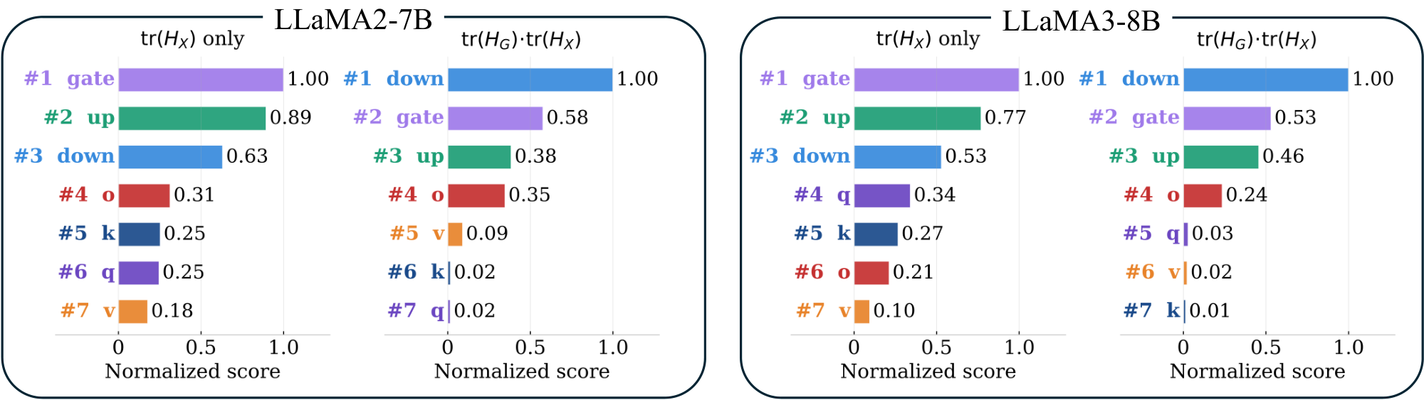
We define the $\textsc{KronQ}$ sensitivity score as $s_\ell = \mathrm{tr}(\mathbf{H}_G^{(\ell)}) \cdot \mathrm{tr}(\mathbf{H}X^{(\ell)})$, computed post-BiIP, and allocate higher bit-widths to sublayers with larger $s\ell$. Within a transformer attention block, the query (Q), key (K), and value (V) projections share the same input, so $\mathbf{H}_X^{(Q)} = \mathbf{H}_X^{(K)} = \mathbf{H}_X^{(V)}$: any activation-only metric assigns identical sensitivity to all three. The $\textsc{KronQ}$ score breaks this degeneracy via $\mathbf{H}_G$, which differs across Q, K, and V as they receive different downstream gradients. As shown in Figure 3, the sublayer rankings under $\mathrm{tr}(\mathbf{H}_G)\cdot\mathrm{tr}(\mathbf{H}_X)$ differ substantially from those under $\mathrm{tr}(\mathbf{H}_X)$ alone. The $\textsc{KronQ}$ score yields strictly better perplexity–bit-width tradeoffs, as we quantify in Section 5.3.

5. Experiments

Section Summary: In the experiments, KronQ was tested on the LLaMA-2 and LLaMA-3 model families of varying sizes and compared against GPTQ and GPTAQ across weight-only, grouped, and combined weight-activation quantization settings. Performance was measured primarily through perplexity on the WikiText-2 dataset and accuracy on commonsense reasoning tasks, with additional checks on newer models such as Gemma and DeepSeek as well as harder benchmarks. Across these regimes, KronQ consistently delivered lower perplexity and higher accuracy than the baselines, with particularly large gains at very low bit widths where competing methods often failed or diverged.

5.1 Experimental Setup

We evaluate $\textsc{KronQ}$ on the LLaMA family, from LLaMA-2-7B/13B/70B ([2]) to LLaMA-3-8B/70B ([3]). We compare against GPTQ ([10]) and GPTAQ ([12]) as primary baselines. We consider three regimes: (i) weight-only quantization (WxA16), (ii) group quantization (WxA16, $g{=}128$), and (iii) weight-and-activation quantization (WxA4). For activation quantization, we utilize the QuaRot ([17]) framework. All other quantization configurations follow GPTAQ ([12]). Perplexity is measured on WikiText-2 ([36]) and zero-shot accuracy is reported on seven commonsense reasoning benchmarks: PiQA ([37]), Arc-Easy (ArcE), Arc-Challenge (ArcC) ([38]), HellaSwag (HS) ([39]), WinoGrande (WG) ([40]), BoolQ ([41]), and OpenBookQA (OBQA) ([42]). All experiments use 128 calibration samples from WikiText-2 with 2048 context lengths and are run on A100 GPUs. $\mathbf{H}_G$ is precomputed via a single backward pass prior to calibration and loaded layer-by-layer on demand, incurring no additional overhead during quantization. Results for prior works are taken from their respective papers, except for OmniQuant ([43]) zero-shot accuracy, which we reproduce using the official implementation.

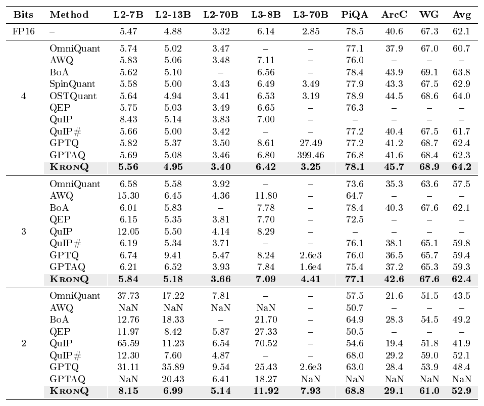
::: {caption="Table 1: Weight-only quantization (WxA16) WikiText-2 perplexity ↓ and zero-shot accuracy ↑ on three reasoning benchmarks (PiQA, ArcC, WG), evaluated on LLaMA-2-7B. NaN indicates diverged quantization, and – indicates results not available. Avg is reported only when all three tasks are available."}

:::

5.2 Results on Uniform Precision

Weight-only Quantization. Table 1 shows WikiText-2 perplexity and zero-shot accuracy on three reasoning benchmarks (PiQA, ArcC, WG) for per-channel weight-only quantization at W4/W3/W2. The comparison baselines include OmniQuant ([43]), AWQ ([19]), BoA ([11]), SpinQuant ([18]), OSTQuant ([26]), QEP ([44]), QuIP ([15]), QuIP# ([16]), GPTQ ([10]), and GPTAQ ([12]). For QuIP#, we report the no-E8P, no-finetuning variant to match our scalar quantization setting. $\textsc{KronQ}$ achieves the lowest perplexity across nearly all settings, with the most significant gains at W2 and W3 where activation-covariance-only methods degrade severely. The zero-shot accuracy improvements mirror the perplexity gains, with $\textsc{KronQ}$ achieving consistently higher accuracy across all benchmarks and bit-widths. On LLaMA-3-70B, GPTQ and GPTAQ diverge or fail to produce valid quantizations, while $\textsc{KronQ}$ achieves 4.41 and 7.93 at W3 and W2, respectively. We attribute this to the anomalously large weight outliers unique to LLaMA-3-70B, as further analyzed in Appendix D. The remaining zero-shot results, comparison with gradient-based methods, and generalization to Mistral-7B are presented in Appendix C.1, Appendix C.2, and Appendix C.3, respectively.

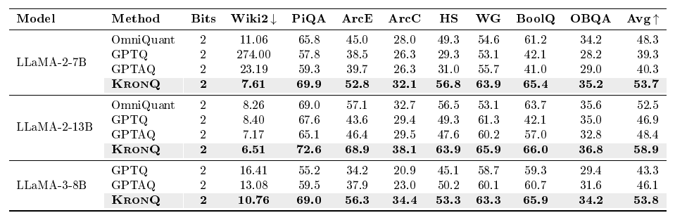
Group Quantization. Group quantization generally achieves better performance than per-channel quantization due to its more optimized scaling factors and zero points. Table 2 reports results under weight-only 2-bit group quantization with 128 column blocks. $\textsc{KronQ}$ maintains its lead over GPTQ and GPTAQ. For example, on LLaMA-2-7B, GPTQ degrades to 274.0 PPL under group quantization while $\textsc{KronQ}$ achieves 7.61. The perplexity comparison with OmniQuant ([43]) and AWQ ([19]) and the results of 3 and 4-bit are shown in Appendix C.4 and Appendix C.5, respectively.

::: {caption="Table 2: Wikitext-2 perplexity and zero-shot accuracy for weight-only group quantization (g=128) at W2."}

:::

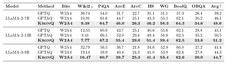
::: {caption="Table 3: Wikitext-2 perplexity and zero-shot accuracy for weight & activation quantization."}

:::

Weight-and-Activation Quantization. For activation quantization, we apply QuaRot ([17]) framework to suppress outliers. Table 3 presents W2A4 results on LLaMA-2-7B/13B and LLaMA-3-8B. $\textsc{KronQ}$ consistently outperforms both baselines across all settings. The gains are again largest at W2A4, where $\textsc{KronQ}$ reduces PPL from 36.74 to 9.38 on LLaMA-2-7B. The comparison with QuaRot ([17]) and SpinQuant ([18]) and other bit-width results are presented in Appendix C.6 and Appendix C.7, respectively.

Generalization to Newer Models and Harder Benchmarks. To verify that KronQ's gains are not specific to the LLaMA family or to perplexity, we evaluate recent model families: Gemma-3-12B ([45]), DeepSeek-R1-Distill-Llama-8B ([46]), and Phi-4-mini-instruct ([47]). Table 4 reports weight-only WikiText-2 perplexity at W4 and W2 against GPTQ ([10]) and GPTAQ ([12]). KronQ wins all eight settings, and the margin widens sharply at W2, confirming that output-side curvature is particularly valuable in the ultra-low-bit regime. Beyond perplexity, Table 5 evaluates four harder benchmarks, GPQA-Diamond ([48]), MMLU ([49]), AIME-2024 ([50]), and LiveCodeBench ([51]) on reasoning models, DeepSeek-R1-Distill-Llama-8B and Gemma-3-12B-IT at W4. KronQ outperforms both baselines on all four benchmarks. The gains are largest on generative reasoning tasks such as LiveCodeBench, where KronQ nearly doubles the GPTAQ scores on both models. Full detailed evaluation settings are provided in Appendix C.8.

\begin{NiceTabular}{l||c|c|c|c}[code-before = \rectanglecolor{gray!15}{2-5}{9-5}]
\toprule
\textbf{Model} & \textbf{Bits} & \textbf{GPTQ} & \textbf{GPTAQ} & \textbf{\textsc{KronQ}} \\
\midrule
\multirow{2}{*}{Gemma-3-12B-PT}
  {} & W4 & 39.77 & 34.84 & \textbf{27.97} \\
  {} & W2 & 1.3e4 & 269.0 & \textbf{60.10} \\
\midrule
\multirow{2}{*}{Gemma-3-12B-IT}
  {} & W4 & 60.37 & 28.82 & \textbf{25.60} \\
  {} & W2 & 7.1e3 & 94.08 & \textbf{54.39} \\
\midrule
\multirow{2}{*}{DeepSeek-R1-Distill-Llama-8B}
  {} & W4 & 16.56 & 15.32 & \textbf{13.58} \\
  {} & W2 & 73.53 & 110.34 & \textbf{27.72} \\
\midrule
\multirow{2}{*}{Phi-4-mini-instruct}
  {} & W4 & 13.81 & 11.80 & \textbf{10.17} \\
  {} & W2 & 111.42 & 31.07 & \textbf{19.26} \\
\bottomrule
\end{NiceTabular}

\begin{NiceTabular}{l|l||c|c|c}[code-before = \rectanglecolor{gray!15}{2-5}{10-5}]
\toprule
\textbf{Model} & \textbf{Benchmark} & \textbf{GPTQ} & \textbf{GPTAQ} & \textbf{\textsc{KronQ}} \\
\midrule
\multirow{4}{*}{\shortstack[l]{DeepSeek-R1-\\Distill-Llama-8B}}
  {} & LiveCodeBench & 19.9 & 16.3 & \textbf{37.3} \\
  {} & AIME-2024 & 10.0 & 13.3 & \textbf{16.7} \\
  {} & MMLU & 44.15 & 40.51 & \textbf{53.17} \\
  {} & GPQA-Diamond & 28.80 & 27.27 & \textbf{29.29} \\
\midrule
\multirow{4}{*}{Gemma-3-12B-IT}
  {} & LiveCodeBench & 7.8 & 9.6 & \textbf{22.3} \\
  {} & AIME-2024 & 10.0 & 10.0 & \textbf{23.3} \\
  {} & MMLU & 64.82 & 65.21 & \textbf{70.02} \\
  {} & GPQA-Diamond & 32.83 & 34.34 & \textbf{38.38} \\
\bottomrule
\end{NiceTabular}

5.3 Results on Mixed-precision

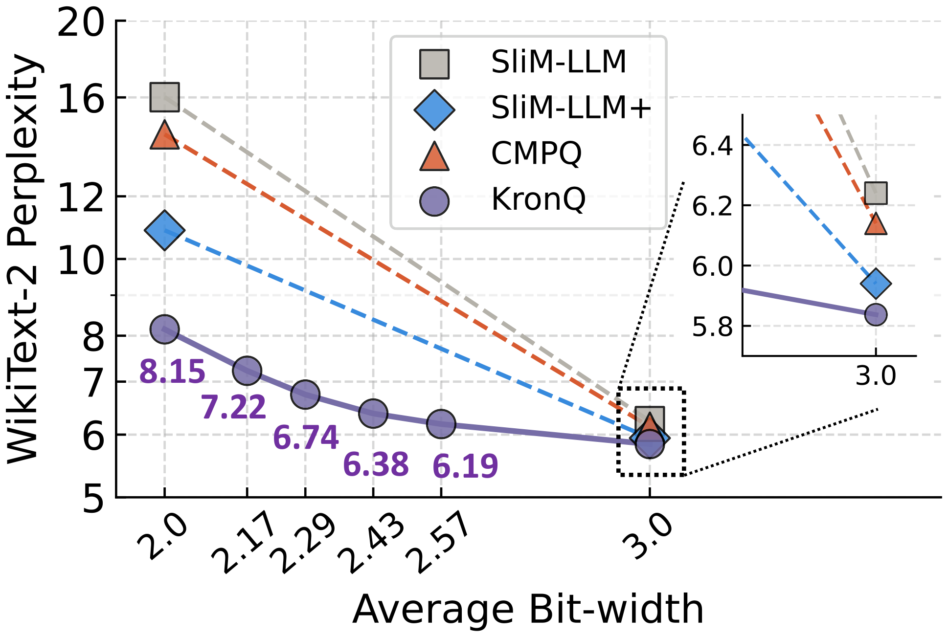
We evaluate the mixed-precision allocation strategy by incrementally upgrading the most sensitive sublayers from W2 to W3 according to the sensitivity score $s = \mathrm{tr}(\mathbf{H}_G) \cdot \mathrm{tr}(\mathbf{H}_X)$ in Equation 14, applying each upgrade across all transformer layers. Table 6 compares the sublayer rankings and WikiText-2 perplexity under the KronQ joint score versus the activation-only score $\mathrm{tr}(\mathbf{H}_X)$ on LLaMA-2-7B. The activation-only score produces suboptimal allocations: its top-1 sublayer (gate_proj) yields higher perplexity than the top-1 of the KronQ joint score (down_proj) at the same average bit-width. The KronQ joint score resolves this degeneracy via $\mathbf{H}_G$, yielding strictly better PPL–bits tradeoff. Figure 4 further compares $\textsc{KronQ}$ mixed-precision against SliM-LLM ([27]), SliM-LLM+, and CMPQ ([28]) on LLaMA-2-7B, demonstrating that $\textsc{KronQ}$ achieves lower perplexity than W3 baselines at only ${\sim}2.6$ average bits. Other architectures show the same trend in Appendix C.9, and a comparison with inter-layer mixed-precision methods is provided in Appendix C.10.

\begin{tabular}{llcc}
\toprule
\textbf{Score} & \textbf{Ranking} & \textbf{Avg bits} & \textbf{Wiki2} $ \!\downarrow$ \\
\midrule
baseline W2 & - & 2.00 & 8.15 \\
\midrule
\multirow{3}{*}{$\mathrm{tr}(H_G)\!\cdot\!\mathrm{tr}(H_X)$} & 1: \texttt{down\_proj} & 2.17 & 7.22 \\
 {} & 2: \texttt{gate\_proj} & 2.29 & 6.74 \\
{} & 3: \texttt{up\_proj} & 2.43 & 6.38 \\
\midrule
\multirow{3}{*}{$\mathrm{tr}(H_X)$} & 1: \texttt{gate\_proj} & 2.17 & 7.45 \\
{} & 2: \texttt{up\_proj} & 2.29 & 6.92 \\
{} & 3: \texttt{down\_proj} & 2.43 & 6.38 \\
\bottomrule
\end{tabular}

5.4 Memory and Latency

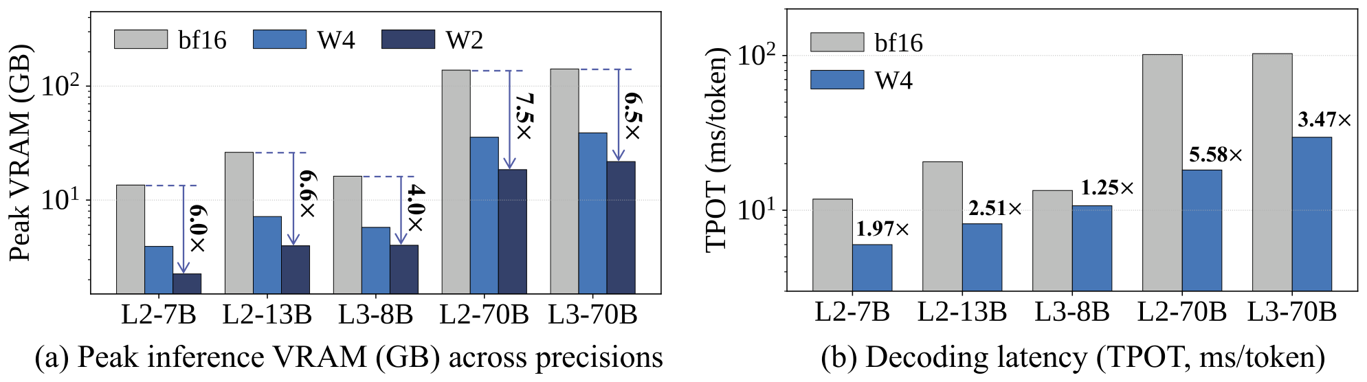
Beyond calibration cost, we measure the end-to-end inference benefit of quantization in Figure 5. On the memory side, KronQ reduces peak inference VRAM by $3.5$ – $3.9\times$ at W4 and $4.0$ – $7.5\times$ at W2 over the bf16 baseline, consistently across model scales. This compression directly translates into deployment enablement: a 70B model that requires two 80 GB A100s in bf16 ($138$ – $141$ GB) fits comfortably on a single A100 at W4 ($35$ – $39$ GB). On the latency side, the reduced memory traffic yields $1.25$ – $2.51\times$ faster decoding, measured as time per output token (TPOT), on the 7B–13B models under a matched single-GPU configuration. We report the 70B latency as well, though its bf16 baseline spans two GPUs and is included only for context.

5.5 Analysis

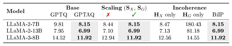
Ablation Study. We conduct three ablation studies to isolate the contribution of each component in $\textsc{KronQ}$, with W2 WikiText-2 perplexity shown in Table 7. First, to isolate the contribution of the base quantizer, we replace GPTAQ with a plain GPTQ base. This degrades perplexity from 8.15/6.99/11.92 to 9.81/7.95/14.52 on LLaMA-2-7B/13B and LLaMA-3-8B, confirming that drift correction and BiIP are complementary. Second, we examine the effect of diagonal rescaling ($\mathbf{S}_X$, $\mathbf{S}_G$) in BiIP. Removing the scaling while retaining the Hadamard rotations consistently degrades perplexity across all models, demonstrating that diagonal rescaling is a necessary complement to the orthogonal transforms. Third, we ablate the rotation directions in BiIP. Applying input-side incoherence ($\mathbf{H}_X$ only) already reduces perplexity, confirming the importance of suppressing input-side outliers ([15]). Output-side incoherence alone ($\mathbf{H}_G$ only) degrades severely on LLaMA-2-7B/13B as input-side outliers remain unaddressed. Combining both directions consistently achieves the lowest perplexity, demonstrating that $\mathbf{H}_G$ provides complementary output-side correction that $\mathbf{H}_X$ alone cannot capture.

::: {caption="Table 7: Ablation study on WikiText-2 perplexity at W2."}

:::

Calibration Efficiency.

\begin{tabular}{llcc}
  \toprule
  Model & Method & Latency & Memory \\
  \midrule
  \multirow{3}{*}{LLaMA-2-7B}
  {} & GPTQ & 24.95 & 1.57 \\
  {} & GPTAQ & 30.11 & 1.99 \\
  {} & \textsc{KronQ} & 38.25 & $3.20 \to 1.99^\dagger$ \\
  \midrule
  \multirow{3}{*}{LLaMA-3-8B}
  {} & GPTQ & 26.13 & 1.97 \\
  {} & GPTAQ & 35.21 & 2.54 \\
  {} & \textsc{KronQ} & 45.59 & $4.38 \to 2.54^\dagger$ \\
  \midrule
  \multirow{3}{*}{LLaMA-2-13B}
  {} & GPTQ & 32.00 & 2.46 \\
  {} & GPTAQ & 39.88 & 3.11 \\
  {} & \textsc{KronQ} & 50.74 & $5.02 \to 3.11^\dagger$ \\
  \bottomrule
  \end{tabular}

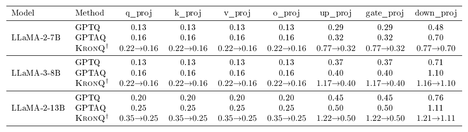
$\textsc{KronQ}$ introduces a moderate latency overhead over GPTAQ (+8–11s/layer across models), attributable to the bidirectional Hadamard rotations in BiIP, which require dense matrix multiplications for both $\mathbf{H}_X$ and $\mathbf{H}G$. This overhead is consistent across model sizes, reflecting that the dominant cost scales with the hidden dimension rather than the total parameter count. For memory, $\textsc{KronQ}$ additionally stores $\mathbf{H}G$ as a full $d\text{out} \times d\text{out}$ matrix during BiIP preprocessing, causing a temporary memory overhead above GPTAQ. However, since $\mathbf{H}_G$ cancels algebraically in the column-wise quantization updates in Proposition 1, it is released upon completion of BiIP, and the memory required for the subsequent quantization loop is identical to GPTAQ. Per-sublayer memory breakdown is provided in Appendix E.

6. Conclusion

Section Summary: The researchers introduced KronQ, a method for reducing the numerical precision of large language models after they have already been trained. It incorporates gradient information to handle certain mathematical inconsistencies across layers and to assign different precision levels where needed, all while keeping the underlying computations efficient. Tests on LLaMA-2 and LLaMA-3 models ranging from 7 billion to 70 billion parameters showed steady gains over prior approaches, especially at the lowest 2-bit settings where other methods tend to fail badly.

We presented $\textsc{KronQ}$, a PTQ framework that incorporates the gradient covariance $\mathbf{H}_G$ into the quantization pipeline. $\textsc{KronQ}$ exploits $\mathbf{H}_G$ for bidirectional incoherence processing and inter-layer mixed-precision allocation, while inheriting the computational efficiency of GPTAQ as $\mathbf{H}_G$ cancels algebraically in the quantization updates. Experiments on LLaMA-2 and LLaMA-3 from 7B to 70B show consistent gains across W2/W3/W4, with the largest improvements at 2-bit, where activation-covariance-only methods degrade severely. The limitations of this work are presented in Appendix F.

Acknowledgments

Section Summary: This research received partial funding from several organizations focused on advancing technology and science. Support came from CoCoSys, a center backed by DARPA and SRC, along with grants from the National Science Foundation and a DARPA award for early-career faculty. Additional resources were provided by a Department of Energy center and an international technology cooperation program.

This work was supported in part by CoCoSys, a JUMP2.0 center sponsored by DARPA and SRC, the National Science Foundation (CAREER Award, Grant #2312366, Grant #2318152), the DARPA Young Faculty Award, the DoE MMICC center SEA-CROGS (Award #DE-SC0023198), and the Global Industrial Technology Cooperation Center (GITCC) program.

Appendix

Section Summary: The appendix presents rigorous mathematical proofs for three key results underlying the KronQ quantization method. The first derives the optimal compensation update for quantized weights by substituting a Kronecker-factored Hessian approximation into the classic optimal brain surgeon formula, showing that the correction simplifies to a simple outer-product adjustment. The second proves that the overall quantization objective remains unchanged under simultaneous orthogonal transformations of the weight matrix and its two Hessian factors, while the third establishes optimality properties of the LDLQ variant by showing that the Kronecker structure preserves an exact LDL factorization and yields a factorized bound on worst-case error.

A. Proofs

A.1 Proof of Proposition 1 (KronQ Weight Compensation)

The general OBS optimal weight update ([7]) is:

$ \Delta\boldsymbol{\theta} = -\mathbf{H}^{-1}\mathbf{E}_p(\mathbf{E}_p^\top\mathbf{H}^{-1}\mathbf{E}_p)^{-1}\delta_p,\tag{15} $

where $\boldsymbol{\theta} = \mathrm{vec}(\mathbf{W})$, $\mathbf{E}_p = \mathbf{I} \otimes e_p$ is the selection matrix for column $p$, and $\delta_p$ is the quantization error. Under the K-FAC approximation $\mathbf{H} = \mathbf{H}_X \otimes \mathbf{H}_G$, we have $\mathbf{H}^{-1} = \mathbf{H}_X^{-1} \otimes \mathbf{H}_G^{-1}$.

We compute the two terms in the OBS formula. First:

$ \begin{aligned} \mathbf{E}_p^\top \mathbf{H}^{-1} \mathbf{E}_p &= (\mathbf{I} \otimes e_p^\top)(\mathbf{H}_X^{-1} \otimes \mathbf{H}_G^{-1})(\mathbf{I} \otimes e_p) \nonumber \ &= [\mathbf{H}_X^{-1}] _{pp} \nonumber \otimes \mathbf{H}_G^{-1} \ &= [\mathbf{H}_X^{-1}] _{pp} \cdot \mathbf{H}_G^{-1}. \end{aligned} $

Second:

$ \mathbf{H}^{-1}\mathbf{E}_p = (\mathbf{H}_X^{-1} \otimes \mathbf{H}_G^{-1})(\mathbf{I} \otimes e_p) = [\mathbf{H}_X^{-1}] _{:, p} \otimes \mathbf{H}_G^{-1}.\tag{16} $

Substituting into the OBS formula, $\mathbf{H}_G^{-1}$ appears in both numerator and denominator and cancels algebraically:

$ \Delta\mathbf{W}_{:, p+1:} = -\frac{[\mathbf{H}_X^{-1}] _{:, p} \otimes \mathbf{H}_G^{-1}}{[\mathbf{H}_X^{-1}] _{pp} \cdot \mathbf{H}_G^{-1}} \cdot \delta_p = -\boldsymbol{\delta}_p \cdot [\mathbf{H}_X^{-1}] _{p, p+1:},\tag{17} $

where $\boldsymbol{\delta}p = (\mathbf{W}{:, p} - \widehat{\mathbf{W}}_{:, p})/[\mathbf{H}_X^{-1}] _{pp}$. Adding the GPTAQ asymmetric correction term ([12]) yields Equation 10. $\square$

A.2 Proof of Theorem 2 (Rotation Invariance)

Denote the transformed quantities after Equation 12 as $\mathbf{W}' = \mathbf{U}\mathbf{W}\mathbf{V}^\top$, $\widetilde{\mathbf{H}}_G = \mathbf{U}\mathbf{H}_G\mathbf{U}^\top$, $\widetilde{\mathbf{H}}_X = \mathbf{V}\mathbf{H}_X\mathbf{V}^\top$, and $(\Delta\mathbf{X}\mathbf{X}^\top)' = \mathbf{V}\Delta\mathbf{X}\mathbf{X}^\top\mathbf{V}^\top$. Note that $\Delta\mathbf{W}' = \mathbf{W}' - \widehat{\mathbf{W}}' = \mathbf{U}\Delta\mathbf{W}\mathbf{V}^\top$. We verify invariance of each term separately.

For the first term:

$ \begin{aligned} \mathrm{tr}!\left[\widetilde{\mathbf{H}}_G, \Delta\mathbf{W}', \widetilde{\mathbf{H}}_X, (\Delta\mathbf{W}')^\top\right] &= \mathrm{tr}!\left[\mathbf{U}\mathbf{H}_G\mathbf{U}^\top \cdot \mathbf{U}\Delta\mathbf{W}\mathbf{V}^\top \cdot \mathbf{V}\mathbf{H}_X\mathbf{V}^\top \cdot \mathbf{V}\Delta\mathbf{W}^\top\mathbf{U}^\top \right] \nonumber \ &= \mathrm{tr}!\left[\mathbf{U}\mathbf{H}_G\Delta\mathbf{W}\mathbf{H}_X\Delta\mathbf{W}^\top\mathbf{U}^\top \right] \nonumber \ &= \mathrm{tr}!\left[\mathbf{H}_G, \Delta\mathbf{W}, \mathbf{H}_X, \Delta\mathbf{W}^\top\right], \end{aligned} $

where the second step uses $\mathbf{U}^\top\mathbf{U} = \mathbf{I}$ and $\mathbf{V}^\top\mathbf{V} = \mathbf{I}$, and the third step uses the cyclic property of the trace.

For the second term:

$ \begin{aligned} \mathrm{tr}!\left[\widetilde{\mathbf{H}}_G, \mathbf{W}', (\Delta\mathbf{X}\mathbf{X}^\top)', (\Delta\mathbf{W}')^\top\right] &= \mathrm{tr}!\left[\mathbf{U}\mathbf{H}_G\mathbf{U}^\top \cdot \mathbf{U}\mathbf{W}\mathbf{V}^\top \cdot \mathbf{V}\Delta\mathbf{X}\mathbf{X}^\top\mathbf{V}^\top \cdot \mathbf{V}\Delta\mathbf{W}^\top\mathbf{U}^\top \right] \nonumber \ &= \mathrm{tr}!\left[\mathbf{U}\mathbf{H}_G, \mathbf{W}, \Delta\mathbf{X}\mathbf{X}^\top, \Delta\mathbf{W}^\top\mathbf{U}^\top \right] \nonumber \ &= \mathrm{tr}!\left[\mathbf{H}_G, \mathbf{W}, \Delta\mathbf{X}\mathbf{X}^\top, \Delta\mathbf{W}^\top\right], \end{aligned} $

where the second step uses $\mathbf{U}^\top\mathbf{U} = \mathbf{I}$ and $\mathbf{V}^\top\mathbf{V} = \mathbf{I}$, and the third step uses the cyclic property of the trace.

Since both terms are individually invariant, the full $\textsc{KronQ}$ objective Equation 9 is invariant under the transformation Equation 12. $\square$

A.3 Proof of Proposition 3 (KronQ-LDLQ Optimality)

Kronecker LDL factorisation.

Let $\mathbf{H}_X = L_X D_X L_X^\top$ and $\mathbf{H}_G = L_G D_G L_G^\top$ be LDL decompositions, where $L_X = U_X + I$ and $L_G = U_G + I$ are unit lower-triangular. Using the mixed-product property of the Kronecker product:

$ \mathbf{H}_X \otimes \mathbf{H}_G = (L_X D_X L_X^\top) \otimes (L_G D_G L_G^\top) = (L_X \otimes L_G)(D_X \otimes D_G)(L_X \otimes L_G)^\top.\tag{18} $

Since $L_X \otimes L_G$ is unit lower-triangular (the Kronecker product of two unit lower-triangular matrices is unit lower-triangular under the standard lexicographic ordering of index pairs), this is a valid LDL decomposition of $\mathbf{H}_X \otimes \mathbf{H}_G$. The diagonal factor is $D_X \otimes D_G$, and:

$ \mathrm{tr}(D_X \otimes D_G) = \sum_{i, j} [D_X] _{ii} [D_G] _{jj} = \mathrm{tr}(D_X)\cdot\mathrm{tr}(D_G).\tag{19} $

Since the worst-case LDLQ proxy loss equals $\frac{1}{4}\mathrm{tr}(D)$ ([15]), it follows that:

$ L_{\mathrm{worst}}(\text{KronQ-LDLQ}) = \frac{1}{4}, \mathrm{tr}(D_X)\cdot\mathrm{tr}(D_G).\tag{20} $

Per-factor incoherence bound.

We apply Lemma 2 of [15] to each Kronecker factor separately. A symmetric positive semidefinite matrix $M \in \mathbb{R}^{n\times n}$ is $\mu$-incoherent if all eigenvectors $v_i$ satisfy $|v_i|_\infty \leq \mu/\sqrt{n}$. For $\mu$-incoherent $M$, QuIP Lemma 2 gives:

$ \mathrm{tr}(D_M) ;\leq; \frac{\mu^2}{n}, \mathrm{tr}(M^{1/2})^2,\tag{21} $

where $D_M$ is the LDL diagonal of $M$. The eigenvectors of $\widetilde{\mathbf{H}}_X \otimes \widetilde{\mathbf{H}}_G$ are $v_i \otimes u_j$ where $v_i$, $u_j$ are eigenvectors of $\widetilde{\mathbf{H}}_X$ and $\widetilde{\mathbf{H}}_G$ respectively. Each entry satisfies $|[v_i \otimes u_j] _k| = |[v_i] {k_1}|\cdot|[u_j] {k_2}| \leq \frac{\mu_X}{\sqrt{d{\mathrm{in}}}}\cdot\frac{\mu_G}{\sqrt{d{\mathrm{out}}}}$, so $\widetilde{\mathbf{H}}X \otimes \widetilde{\mathbf{H}}G$ is $(\mu_X\mu_G)$-incoherent with ambient dimension $d{\mathrm{in}} d{\mathrm{out}}$. Applying the per-factor bound and trace invariance under orthogonal conjugation ($\mathrm{tr}(\widetilde{\mathbf{H}}_X^{1/2}) = \mathrm{tr}(\mathbf{H}_X^{1/2})$, $\mathrm{tr}(\widetilde{\mathbf{H}}_G^{1/2}) = \mathrm{tr}(\mathbf{H}_G^{1/2})$):

$ \frac{1}{4}, \mathrm{tr}(D_X)\cdot\mathrm{tr}(D_G) ;\leq; \frac{\mu_X^2, \mu_G^2}{4, d_{\mathrm{in}}, d_{\mathrm{out}}} \cdot\mathrm{tr}(\mathbf{H}_X^{1/2})^2, \mathrm{tr}(\mathbf{H}_G^{1/2})^2.\tag{22} $

Finally, applying $\mathrm{tr}(H^{1/2})^2 \leq \mathrm{rank}(H)\cdot\mathrm{tr}(H)$ to each factor (by Cauchy–Schwarz on the eigenvalues) gives:

$ \frac{\mu_X^2, \mu_G^2}{4, d_{\mathrm{in}}, d_{\mathrm{out}}} \cdot\mathrm{tr}(\mathbf{H}X^{1/2})^2, \mathrm{tr}(\mathbf{H}G^{1/2})^2 ;\leq; \frac{\mu_X^2, \mu_G^2, k_X, k_G}{4, d{\mathrm{in}}, d{\mathrm{out}}} \cdot\mathrm{tr}(\mathbf{H}_X), \mathrm{tr}(\mathbf{H}_G),\tag{23} $

where $k_X = \mathrm{rank}(\mathbf{H}_X)$ and $k_G = \mathrm{rank}(\mathbf{H}_G)$. $\square$

Comparison with QuIP.

Setting $\mathbf{H}G = \mathbf{I}$ (rank- $d{\mathrm{out}}$, $\mu_G = 1$, $k_G = d_{\mathrm{out}}$) recovers the QuIP ([15]) bound $\mu_X^2 k_X, \mathrm{tr}(\mathbf{H}X) / (4 d{\mathrm{in}})$. KronQ+BiIP improves this bound by the factor $\mu_G^2 k_G / d_{\mathrm{out}}$, which can be substantially less than one when $\mathbf{H}_G$ is approximately low-rank.

\begin{tabular}{lc}
\toprule
\textbf{Method} & \textbf{Worst-case proxy loss} \\
\midrule
Nearest rounding & $\tfrac{1}{4}\, \mathrm{tr}(\mathbf{H}_X)\cdot\mathrm{tr}(\mathbf{H}_G)$ \\ 
GPTQ-LDLQ ($\mathbf{H}_G = \mathbf{I}$) & $\tfrac{1}{4}\, \mathrm{tr}(D_X)\cdot d_{\mathrm{out}}$ \\
KronQ-LDLQ (ours) & $\tfrac{1}{4}\, \mathrm{tr}(D_X)\cdot\mathrm{tr}(D_G)$ \\
\bottomrule
\end{tabular}

B. KronQ Algorithm

**Require:** FP weight $\mathbf{W} \in \mathbb{R}^{d_\mathrm{out} \times d_\mathrm{in}}$,
degraded input $\mathbf{X} \in \mathbb{R}^{d_\mathrm{in} \times n}$,
FP input $\tilde{\mathbf{X}} \in \mathbb{R}^{d_\mathrm{in} \times n}$,
$\mathbf{H}_G \in \mathbb{R}^{d_\mathrm{out} \times d_\mathrm{out}}$ (precomputed)
$\mathbf{H}_X \leftarrow \mathbf{X}\mathbf{X}^\top$;
$\Delta\mathbf{X}\mathbf{X}^\top \leftarrow (\tilde{\mathbf{X}} - \mathbf{X})\mathbf{X}^\top$
// online statistics
**sample** random Hadamard $\mathbf{U} \in \mathbb{R}^{d_\mathrm{out} \times d_\mathrm{out}}$,
$\mathbf{V} \in \mathbb{R}^{d_\mathrm{in} \times d_\mathrm{in}}$
$\mathbf{S}_X \leftarrow \bigl(\mathrm{diag}(\mathbf{H}_X) / \mathrm{diag}(\mathbf{W}^\top \mathbf{W})\bigr)^{1/4}$
// input-side rescaling
$\mathbf{S}_G \leftarrow \bigl(\mathrm{diag}(\mathbf{H}_G) / \mathrm{diag}(\mathbf{W}\mathbf{W}^\top)\bigr)^{1/4}$
// output-side rescaling
$\mathbf{W} \leftarrow \mathbf{S}_G\,\mathbf{W}\,\mathbf{S}_X$
$\mathbf{H}_X \leftarrow \mathbf{S}_X^{-1}\mathbf{H}_X\mathbf{S}_X^{-1}$;
$\Delta\mathbf{X}\mathbf{X}^\top \leftarrow \mathbf{S}_X^{-1}\Delta\mathbf{X}\mathbf{X}^\top\mathbf{S}_X^{-1}$;
$\mathbf{H}_G \leftarrow \mathbf{S}_G^{-1}\mathbf{H}_G\mathbf{S}_G^{-1}$
$\mathbf{W} \leftarrow \mathbf{U}\mathbf{W}\mathbf{V}^\top$;
$\mathbf{H}_X \leftarrow \mathbf{V}\mathbf{H}_X\mathbf{V}^\top$;
$\Delta\mathbf{X}\mathbf{X}^\top \leftarrow \mathbf{V}\,\Delta\mathbf{X}\mathbf{X}^\top\mathbf{V}^\top$
// incoherence
$\mathbf{H}_G \leftarrow \mathbf{U}\mathbf{H}_G\mathbf{U}^\top$; **release** $\mathbf{H}_G$
// $\mathbf{H}_G$ not needed after BiIP (Prop. 1)
**return** $\mathbf{W},\;\mathbf{H}_X,\;\Delta\mathbf{X}\mathbf{X}^\top,\;\mathbf{S}_X,\;\mathbf{S}_G,\;\mathbf{U},\;\mathbf{V}$

**Require:** $\mathbf{W} \in \mathbb{R}^{m \times n},\, \mathbf{H}_X \in \mathbb{R}^{n \times n},\, \Delta\mathbf{X}\mathbf{X}^\top \in \mathbb{R}^{n \times n},\, \mathbf{S}_X,\, \mathbf{S}_G,\, \mathbf{U},\, \mathbf{V}$
(from Alg. Algorithm 1),
block size B, damping $\lambda$, scaling $\alpha$
$\mathbf{H}_X \leftarrow \mathbf{H}_X + \lambda \cdot \mathrm{mean}(\mathrm{diag}(\mathbf{H}_X))\,\mathbf{I}$
// damping
$\mathbf{L} \leftarrow \textit{Inverse\_Cholesky}(\mathbf{H}_X)$
$\mathbf{P} \leftarrow \alpha\bigl((\Delta\mathbf{X}\mathbf{X}^\top \cdot \mathbf{L}) \odot \mathbf{M}_U\bigr)\mathbf{L}^\top$
// GPTAQ correction; $\mathbf{M}_U$: upper-triangular mask
$\mathbf{Q} \leftarrow \mathbf{0}_{m \times n}$;
$\mathbf{E} \leftarrow \mathbf{0}_{m \times B}$
**for** i = 0, B, 2B, … **do**
  **for** j = i, i+1, …, i+B-1 **do**
    $\mathbf{Q}_{:,j} \leftarrow \mathrm{quant}(\mathbf{W}_{:,j})$
    $\mathbf{E}_{:,\,j-i} \leftarrow (\mathbf{W}_{:,j} - \mathbf{Q}_{:,j})\;/\;\mathbf{L}_{jj}$
    $\mathbf{W}_{:,\,j:(i+B)} \leftarrow \mathbf{W}_{:,\,j:(i+B)} - \mathbf{E}_{:,\,j-i}\,\mathbf{L}_{j,\,j:(i+B)}^\top + \mathbf{W}_{:,j}\,\mathbf{P}_{j,\,j:(i+B)}$
  **end for**
  $\mathbf{W}_{:,\,(i+B):} \leftarrow \mathbf{W}_{:,\,(i+B):} - \mathbf{E}\cdot\mathbf{L}_{i:(i+B),\,(i+B):}^\top + \mathbf{W}_{:,\,i:(i+B)}\,\mathbf{P}_{i:(i+B),\,(i+B):}$
**end for**
$\mathbf{Q} \leftarrow \mathbf{U}^\top \mathbf{Q}\,\mathbf{V}$;
$\mathbf{Q} \leftarrow \mathbf{S}_G^{-1}\,\mathbf{Q}\,\mathbf{S}_X^{-1}$
// revert incoherence \& rescaling
**return** $\mathbf{Q}$

C. Additional Experiments

C.1 Zero-shot Accuracy on Weight-only Quantization

\begin{longtable}{l||l|c|cccccccr}

\\

\hline
\textbf{Model} & \textbf{Method} & \textbf{Bits}
   {} & \textbf{PiQA} & \textbf{ArcE} & \textbf{ArcC} & \textbf{HS}
   {} & \textbf{WG} & \textbf{BoolQ} & \textbf{OBQA}
   {} & \textbf{Avg} $\!\uparrow$ \\
\hline
\midrule
\endfirsthead

\hline
\endlastfoot

\multirow{13}{*}{LLaMA-2-7B}
  {} & GPTQ & 4 & 77.2 & 69.2 & 41.2 & 70.5 & 68.7 & 67.3 & 40.8 & 62.1 \\
  {} & GPTAQ & 4 & 76.8 & 70.6 & 41.6 & 70.3 & 68.4 & 68.1 & 42.6 & 62.6 \\
  {} & \cellcolor{gray!15}\textbf{\textsc{KronQ}} & \cellcolor{gray!15}\textbf{4} & \cellcolor{gray!15}\textbf{78.1} & \cellcolor{gray!15}\textbf{73.7} & \cellcolor{gray!15}\textbf{45.7} & \cellcolor{gray!15}\textbf{75.2} & \cellcolor{gray!15}\textbf{68.9} & \cellcolor{gray!15}\textbf{78.1} & \cellcolor{gray!15}\textbf{43.6} & \cellcolor{gray!15}\textbf{66.2} \\
\cline{2-11}
  {} & OmniQuant & 3 & 74.0 & 62.6 & 36.3 & 67.6 & 63.6 & 65.7 & 39.8 & 58.5 \\
  {} & GPTQ & 3 & 76.0 & 59.4 & 36.5 & 66.8 & 65.7 & 65.9 & 40.0 & 58.6 \\
  {} & BoA & 3 & 78.4 & 69.3 & 40.3 & 72.0 & 67.6 & 74.2 & 41.2 & 63.3 \\
  {} & GPTAQ & 3 & 75.4 & 62.0 & 37.2 & 65.9 & 65.3 & 66.1 & 38.4 & 58.6 \\
  {} & \cellcolor{gray!15}\textbf{\textsc{KronQ}} & \cellcolor{gray!15}\textbf{3} & \cellcolor{gray!15}\textbf{77.1} & \cellcolor{gray!15}\textbf{72.4} & \cellcolor{gray!15}\textbf{42.6} & \cellcolor{gray!15}\textbf{72.0} & \cellcolor{gray!15}\textbf{67.6} & \cellcolor{gray!15}\textbf{75.4} & \cellcolor{gray!15}\textbf{41.6} & \cellcolor{gray!15}\textbf{64.1} \\
\cline{2-11}
  {} & OmniQuant & 2 & 57.2 & 35.3 & 26.1 & 31.7 & 51.5 & 51.1 & 30.6 & 40.5 \\
  {} & GPTQ & 2 & 63.0 & 45.1 & 28.4 & 42.8 & 53.9 & 52.3 & 28.4 & 44.8 \\
  {} & BoA & 2 & 64.9 & 47.7 & 28.3 & 45.5 & 54.5 & 64.7 & 29.6 & 47.9 \\
  {} & GPTAQ & 2 & NaN & NaN & NaN & NaN & NaN & NaN & NaN & NaN \\
  {} & \cellcolor{gray!15}\textbf{\textsc{KronQ}} & \cellcolor{gray!15}\textbf{2} & \cellcolor{gray!15}\textbf{68.8} & \cellcolor{gray!15}\textbf{55.0} & \cellcolor{gray!15}\textbf{29.1} & \cellcolor{gray!15}\textbf{52.3} & \cellcolor{gray!15}\textbf{61.0} & \cellcolor{gray!15}\textbf{62.7} & \cellcolor{gray!15}\textbf{35.0} & \cellcolor{gray!15}\textbf{52.0} \\
\hline
\multirow{13}{*}{LLaMA-2-13B}
  {} & GPTQ & 4 & 77.3 & 73.7 & 45.6 & 67.6 & 71.1 & 71.0 & 43.2 & 64.2 \\
  {} & GPTAQ & 4 & 77.9 & 74.4 & 46.5 & 73.1 & 71.3 & 75.5 & 44.8 & 66.2 \\
  {} & \cellcolor{gray!15}\textbf{\textsc{KronQ}} & \cellcolor{gray!15}\textbf{4} & \cellcolor{gray!15}\textbf{80.2} & \cellcolor{gray!15}\textbf{74.7} & \cellcolor{gray!15}\textbf{48.0} & \cellcolor{gray!15}\textbf{79.1} & \cellcolor{gray!15}\textbf{71.8} & \cellcolor{gray!15}\textbf{82.1} & \cellcolor{gray!15}\textbf{44.8} & \cellcolor{gray!15}\textbf{68.7} \\
\cline{2-11}
  {} & OmniQuant & 3 & 77.7 & 69.0 & 42.7 & 72.8 & 65.9 & 69.0 & 38.8 & 62.3 \\
  {} & GPTQ & 3 & 72.5 & 62.8 & 36.8 & 54.4 & 65.5 & 66.5 & 36.6 & 56.4 \\
  {} & BoA & 3 & 77.4 & 69.3 & 43.5 & 74.7 & 62.5 & 78.9 & 35.2 & 63.1 \\
  {} & GPTAQ & 3 & 75.1 & 65.5 & 39.0 & 62.6 & 64.2 & 67.3 & 38.2 & 58.8 \\
  {} & \cellcolor{gray!15}\textbf{\textsc{KronQ}} & \cellcolor{gray!15}\textbf{3} & \cellcolor{gray!15}\textbf{79.3} & \cellcolor{gray!15}\textbf{73.5} & \cellcolor{gray!15}\textbf{46.5} & \cellcolor{gray!15}\textbf{77.0} & \cellcolor{gray!15}\textbf{71.2} & \cellcolor{gray!15}\textbf{78.9} & \cellcolor{gray!15}\textbf{45.0} & \cellcolor{gray!15}\textbf{67.3} \\
\cline{2-11}
  {} & OmniQuant & 2 & 62.9 & 44.4 & 28.4 & 49.7 & 52.6 & 62.2 & 33.8 & 47.7 \\
  {} & GPTQ & 2 & 57.9 & 36.2 & 23.4 & 37.3 & 53.2 & 62.1 & 28.2 & 42.6 \\
  {} & BoA & 2 & 63.3 & 46.3 & 29.8 & 49.3 & 52.6 & 62.2 & 27.6 & 47.3 \\
  {} & GPTAQ & 2 & 54.8 & 33.1 & 21.4 & 31.7 & 52.0 & 58.0 & 29.4 & 40.1 \\
  {} & \cellcolor{gray!15}\textbf{\textsc{KronQ}} & \cellcolor{gray!15}\textbf{2} & \cellcolor{gray!15}\textbf{72.4} & \cellcolor{gray!15}\textbf{62.5} & \cellcolor{gray!15}\textbf{36.4} & \cellcolor{gray!15}\textbf{59.4} & \cellcolor{gray!15}\textbf{65.1} & \cellcolor{gray!15}\textbf{69.4} & \cellcolor{gray!15}\textbf{37.0} & \cellcolor{gray!15}\textbf{57.5} \\
\hline
\multirow{11}{*}{LLaMA-2-70B}
  {} & GPTQ & 4 & 82.3 & 81.0 & 57.6 & 82.7 & 77.4 & 82.3 & 48.0 & 73.0 \\
  {} & GPTAQ & 4 & 82.8 & 81.5 & 57.3 & 82.8 & 77.0 & 82.4 & 47.8 & 73.1 \\
  {} & \cellcolor{gray!15}\textbf{\textsc{KronQ}} & \cellcolor{gray!15}\textbf{4} & \cellcolor{gray!15}\textbf{82.3} & \cellcolor{gray!15}\textbf{80.3} & \cellcolor{gray!15}\textbf{57.9} & \cellcolor{gray!15}\textbf{83.8} & \cellcolor{gray!15}\textbf{79.9} & \cellcolor{gray!15}\textbf{85.4} & \cellcolor{gray!15}\textbf{49.2} & \cellcolor{gray!15}\textbf{74.1} \\
\cline{2-11}
  {} & OmniQuant & 3 & 80.7 & 75.6 & 45.8 & 78.1 & 73.6 & 66.5 & 42.6 & 66.1 \\
  {} & GPTQ & 3 & 80.4 & 78.9 & 55.8 & 80.2 & 76.2 & 79.1 & 46.0 & 70.9 \\
  {} & GPTAQ & 3 & 81.7 & 77.5 & 54.4 & 79.8 & 75.2 & 81.6 & 45.8 & 70.9 \\
  {} & \cellcolor{gray!15}\textbf{\textsc{KronQ}} & \cellcolor{gray!15}\textbf{3} & \cellcolor{gray!15}\textbf{82.3} & \cellcolor{gray!15}\textbf{81.9} & \cellcolor{gray!15}\textbf{58.3} & \cellcolor{gray!15}\textbf{82.5} & \cellcolor{gray!15}\textbf{78.5} & \cellcolor{gray!15}\textbf{83.0} & \cellcolor{gray!15}\textbf{48.8} & \cellcolor{gray!15}\textbf{73.6} \\
\cline{2-11}
  {} & OmniQuant & 2 & 69.9 & 55.5 & 31.5 & 55.4 & 53.6 & 64.9 & 33.8 & 52.1 \\
  {} & GPTQ & 2 & 72.1 & 64.7 & 37.6 & 58.0 & 66.9 & 66.6 & 40.2 & 58.0 \\
  {} & GPTAQ & 2 & 72.2 & 64.4 & 36.8 & 58.4 & 64.6 & 69.9 & 34.6 & 57.3 \\
  {} & \cellcolor{gray!15}\textbf{\textsc{KronQ}} & \cellcolor{gray!15}\textbf{2} & \cellcolor{gray!15}\textbf{77.4} & \cellcolor{gray!15}\textbf{75.9} & \cellcolor{gray!15}\textbf{46.9} & \cellcolor{gray!15}\textbf{72.0} & \cellcolor{gray!15}\textbf{75.0} & \cellcolor{gray!15}\textbf{79.7} & \cellcolor{gray!15}\textbf{43.2} & \cellcolor{gray!15}\textbf{67.2} \\
\hline
\multirow{11}{*}{LLaMA-3-8B}
  {} & GPTQ & 4 & 79.4 & 75.7 & 49.7 & 75.6 & 73.5 & 77.1 & 44.8 & 68.0 \\
  {} & GPTAQ & 4 & 80.0 & 75.7 & 49.7 & 77.2 & 72.5 & 76.5 & 44.4 & 68.0 \\
  {} & \cellcolor{gray!15}\textbf{\textsc{KronQ}} & \cellcolor{gray!15}\textbf{4} & \cellcolor{gray!15}\textbf{79.4} & \cellcolor{gray!15}\textbf{78.2} & \cellcolor{gray!15}\textbf{51.5} & \cellcolor{gray!15}\textbf{78.2} & \cellcolor{gray!15}\textbf{73.2} & \cellcolor{gray!15}\textbf{82.2} & \cellcolor{gray!15}\textbf{44.2} & \cellcolor{gray!15}\textbf{69.6} \\
\cline{2-11}
  {} & GPTQ & 3 & 74.5 & 62.6 & 39.7 & 70.0 & 67.8 & 73.3 & 38.6 & 60.9 \\
  {} & BoA & 3 & 77.3 & 72.8 & 45.1 & 72.7 & 71.4 & 78.7 & 42.6 & 65.8 \\
  {} & GPTAQ & 3 & 73.5 & 60.1 & 40.4 & 70.8 & 69.9 & 75.7 & 41.0 & 61.6 \\
  {} & \cellcolor{gray!15}\textbf{\textsc{KronQ}} & \cellcolor{gray!15}\textbf{3} & \cellcolor{gray!15}\textbf{77.5} & \cellcolor{gray!15}\textbf{74.5} & \cellcolor{gray!15}\textbf{50.2} & \cellcolor{gray!15}\textbf{74.9} & \cellcolor{gray!15}\textbf{71.7} & \cellcolor{gray!15}\textbf{81.1} & \cellcolor{gray!15}\textbf{41.2} & \cellcolor{gray!15}\textbf{67.3} \\
\cline{2-11}
  {} & GPTQ & 2 & 54.2 & 34.0 & 22.3 & 37.9 & 49.5 & 45.9 & 28.0 & 38.8 \\
  {} & BoA & 2 & 59.9 & 44.9 & 26.6 & 43.3 & 55.8 & 60.5 & 29.4 & 45.8 \\
  {} & GPTAQ & 2 & 55.0 & 33.1 & 23.6 & 38.1 & 53.4 & 46.8 & 28.0 & 39.7 \\
  {} & \cellcolor{gray!15}\textbf{\textsc{KronQ}} & \cellcolor{gray!15}\textbf{2} & \cellcolor{gray!15}\textbf{67.0} & \cellcolor{gray!15}\textbf{50.7} & \cellcolor{gray!15}\textbf{30.6} & \cellcolor{gray!15}\textbf{49.0} & \cellcolor{gray!15}\textbf{61.1} & \cellcolor{gray!15}\textbf{66.1} & \cellcolor{gray!15}\textbf{33.0} & \cellcolor{gray!15}\textbf{51.1} \\
\hline
\multirow{9}{*}{LLaMA-3-70B}
  {} & GPTQ & 4 & 50.2 & 26.3 & 24.6 & 59.8 & 56.4 & 66.9 & 33.2 & 45.3 \\
  {} & GPTAQ & 4 & 56.9 & 39.6 & 25.6 & 30.1 & 54.4 & 48.1 & 29.0 & 40.5 \\
  {} & \cellcolor{gray!15}\textbf{\textsc{KronQ}} & \cellcolor{gray!15}\textbf{4} & \cellcolor{gray!15}\textbf{84.2} & \cellcolor{gray!15}\textbf{81.8} & \cellcolor{gray!15}\textbf{61.7} & \cellcolor{gray!15}\textbf{84.8} & \cellcolor{gray!15}\textbf{79.1} & \cellcolor{gray!15}\textbf{86.8} & \cellcolor{gray!15}\textbf{48.0} & \cellcolor{gray!15}\textbf{75.2} \\
\cline{2-11}
  {} & GPTQ & 3 & 52.0 & 25.3 & 26.1 & 26.4 & 49.0 & 41.2 & 28.4 & 35.5 \\
  {} & GPTAQ & 3 & 50.0 & 25.9 & 27.5 & 26.2 & 49.7 & 37.9 & 30.0 & 35.3 \\
  {} & \cellcolor{gray!15}\textbf{\textsc{KronQ}} & \cellcolor{gray!15}\textbf{3} & \cellcolor{gray!15}\textbf{83.5} & \cellcolor{gray!15}\textbf{80.4} & \cellcolor{gray!15}\textbf{58.8} & \cellcolor{gray!15}\textbf{83.1} & \cellcolor{gray!15}\textbf{79.5} & \cellcolor{gray!15}\textbf{85.4} & \cellcolor{gray!15}\textbf{47.2} & \cellcolor{gray!15}\textbf{74.0} \\
\cline{2-11}
  {} & GPTQ & 2 & 51.7 & 25.6 & 26.4 & 26.4 & 49.0 & 37.8 & 27.4 & 34.9 \\
  {} & GPTAQ & 2 & NaN & NaN & NaN & NaN & NaN & NaN & NaN & NaN \\
  {} & \cellcolor{gray!15}\textbf{\textsc{KronQ}} & \cellcolor{gray!15}\textbf{2} & \cellcolor{gray!15}\textbf{77.6} & \cellcolor{gray!15}\textbf{73.2} & \cellcolor{gray!15}\textbf{44.5} & \cellcolor{gray!15}\textbf{66.0} & \cellcolor{gray!15}\textbf{72.6} & \cellcolor{gray!15}\textbf{79.1} & \cellcolor{gray!15}\textbf{39.6} & \cellcolor{gray!15}\textbf{64.7} \\
\hline
\end{longtable}

C.2 Comparison with Gradient-Based Methods

YAQA ([13]) shares the K-FAC form $\mathbf{H} \approx \mathbf{H}_X \otimes \mathbf{H}_G$ but folds $\mathbf{H_G}$ into a modified LDLQ solver, whereas KronQ uses $\mathbf{H_G}$ only for incoherence and bit allocation. Table 11 shows that KronQ attains lower perplexity at an order-of-magnitude lower calibration cost. GuidedQuant ([14]) weights the input-side Hessian by per-output-channel saliency, missing the cross-output-channel structure that $\mathbf{H_G}$ captures. As shown in Table 12, KronQ matches or exceeds its LNQ-based results with a plain uniform per-channel grid.

\begin{tabular}{lc}
\toprule
Method & WikiText-2 PPL \\
\midrule
BF16 & 6.50 \\
LDLQ & 6.76 \\
YAQA-A & 6.71 \\
YAQA-B & 6.72 \\
\cellcolor{gray!15}\textbf{KronQ} & \cellcolor{gray!15}\textbf{6.69} \\
\bottomrule
\end{tabular}

\begin{NiceTabular}{llcc}[code-before = \rectanglecolor{gray!15}{2-4}{7-4}]
\toprule
Model & Bits & LNQ+GuidedQuant & \textbf{KronQ} \\
\midrule
L2-7B & W3 & 5.57 & \textbf{5.44} \\
L2-13B & W3 & 4.91 & \textbf{4.84} \\
L2-70B & W3 & 3.47 & \textbf{3.48} \\
\midrule
L2-7B & W2 & 8.83 & \textbf{7.64} \\
L2-13B & W2 & 7.26 & \textbf{6.50} \\
L2-70B & W2 & 5.04 & \textbf{5.07} \\
\bottomrule
\end{NiceTabular}

C.3 Comparison on Mistral-7B

Table 13 extends the weight-only quantization evaluation to Mistral-7B ([52]), demonstrating that $\textsc{KronQ}$ generalizes beyond the LLaMA family.

\begin{NiceTabular}{lcccccc}[code-before = \rectanglecolor{gray!15}{2-7}{5-7}]
\toprule
  {} & AWQ & QEP & QuIP & GPTQ & GPTAQ & \textbf{\textsc{KronQ}} \\
\midrule
W4 & 5.72 & 5.48 & 11.11 & 8.96 & 6.95 & \textbf{5.32} \\
W3 & 7.90 & 5.84 & 7.11 & 532.46 & 12.89 & \textbf{5.54} \\
W2 & NaN & 9.59 & 26.63 & 5900.69 & 27.07 & \textbf{7.78} \\
\bottomrule
\end{NiceTabular}

C.4 Comparison with Previous Works on Group Quantization

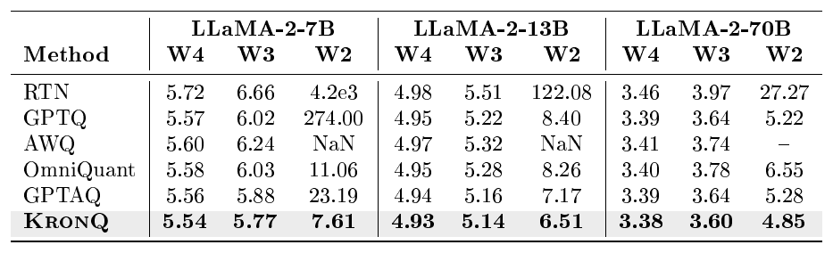
Table 14 reports WikiText-2 perplexity under group quantization ($g{=}128$), where OmniQuant ([43]) and AWQ ([19]) results are taken from their papers.

::: {caption="Table 14: Weight-only group quantization (WxA16, g=128) WikiText-2 perplexity."}

:::

C.5 3 and 4-bit Results on Group Quantization

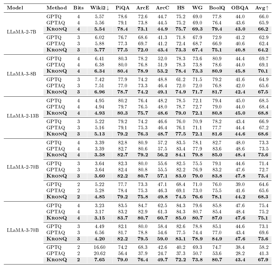
Table 15 provides full W2/W3/W4 results under group quantization ($g{=}128$). $\textsc{KronQ}$ maintains its lead across all bit-widths and model sizes, with particularly large margins at W2 where per-channel methods struggle.

::: {caption="Table 15: Group quantization (WxA16, g=128), full results (W2/W3/W4)."}

:::

C.6 Comparison with Previous Works on Weight-and-activation Quantization

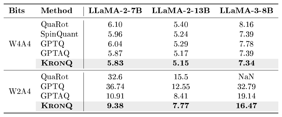
Table 16 reports WikiText-2 perplexity for weight-and-activation quantization. All methods apply the QuaRot ([17]) rotation framework for activation quantization. QuaRot and SpinQuant ([18]) results are taken from their respective papers.

::: {caption="Table 16: Weight-and-activation quantization (WxA4) WikiText-2 perplexity."}

:::

C.7 3 and 4-bit Results on Weight-and-activation Quantization

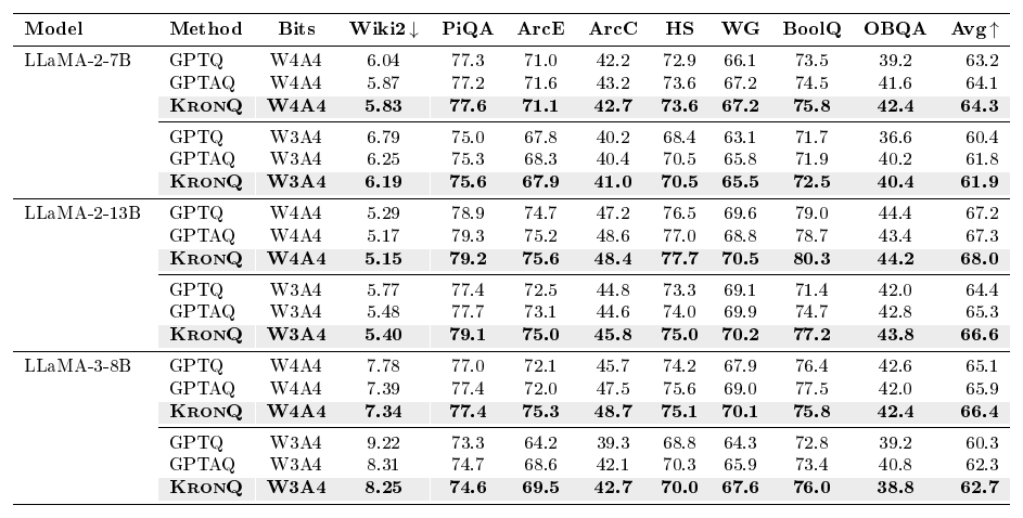
Table 17 extends the weight-and-activation evaluation to W3A4/W4A4. $\textsc{KronQ}$ achieves the lowest perplexity across all settings, with gains increasing at lower bit-widths.

::: {caption="Table 17: Weight-and-activation quantization (WxA4), W3A4/W4A4 results."}

:::

C.8 Harder Benchmark Evaluation Details

We evaluate DeepSeek-R1-Distill-Llama-8B ([46]) and Gemma-3-12B-IT ([45]), each quantized to W4 (per-channel, asymmetric, weight-only) with KronQ and, as baselines, with GPTQ and GPTAQ under identical settings. All models are calibrated on 128 WikiText-2 sequences with no fine-tuning. MMLU, GPQA-Diamond, and AIME-2024 are evaluated through the lm-evaluation-harness ([53]) in the zero-shot setting, while LiveCodeBench uses its official runner with vLLM. We report log-likelihood accuracy on MMLU (57 subjects) and GPQA-Diamond (198 questions), exact-match accuracy on AIME-2024 (30 problems), and pass@1 on LiveCodeBench (release_v5, code-generation scenario, 32,768 maximum new tokens). For the reasoning model DeepSeek-R1-Distill-Llama-8B, we follow the decoding protocol of [54], using temperature 0.6, top-p 0.95, and 32,768 maximum new tokens with stochastic sampling. We report its AIME-2024 score averaged over 8 samples (avg@8). The instruction-tuned Gemma-3-12B-IT is decoded greedily with a 2,048-token budget, and we report its AIME-2024 as pass@1.

C.9 Mixed Precision Quantization on LLaMA

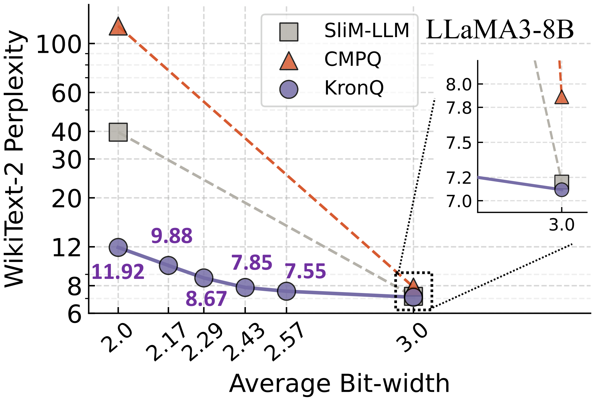
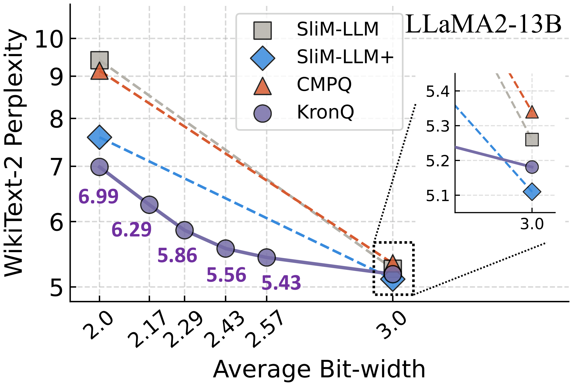
Table 18 and right figures extend the mixed-precision analysis of Section 5.3 to LLaMA-3-8B and LLaMA-2-13B. The KronQ joint score yields strictly better PPL–bits tradeoffs than the activation-only score on both architectures. We also compare $\textsc{KronQ}$ with SliM-LLM ([27]) and CMPQ ([28]), consistent with the LLaMA-2-7B results in the main paper.

\begin{tabular}{llcc}
\toprule
\textbf{Score} & \textbf{Ranking} & \textbf{Avg bits} & \textbf{Wiki2} $\!\downarrow$ \\
\midrule
\multicolumn{4}{l}{\textit{LLaMA-3-8B}} \\
\midrule
baseline W2 & - & 2.00 & 11.92 \\
\midrule
\multirow{3}{*}{$\mathrm{tr}(H_G)\!\cdot\!\mathrm{tr}(H_X)$} & 1: \texttt{down\_proj} & 2.17 & 9.88 \\
 {} & 2: \texttt{gate\_proj} & 2.29 & 8.67 \\
 {} & 3: \texttt{up\_proj} & 2.43 & 7.85 \\
\midrule
\multirow{3}{*}{$\mathrm{tr}(H_X)$} & 1: \texttt{gate\_proj} & 2.17 & 10.24 \\
 {} & 2: \texttt{up\_proj} & 2.29 & 9.16 \\
 {} & 3: \texttt{down\_proj} & 2.43 & 7.85 \\
\midrule
\multicolumn{4}{l}{\textit{LLaMA-2-13B}} \\
\midrule
baseline W2 & - & 2.00 & 6.99 \\
\midrule
\multirow{3}{*}{$\mathrm{tr}(H_G)\!\cdot\!\mathrm{tr}(H_X)$} & 1: \texttt{down\_proj} & 2.17 & 6.29 \\
 {} & 2: \texttt{gate\_proj} & 2.29 & 5.86 \\
 {} & 3: \texttt{up\_proj} & 2.43 & 5.56 \\
\midrule
\multirow{3}{*}{$\mathrm{tr}(H_X)$} & 1: \texttt{gate\_proj} & 2.17 & 6.39 \\
 {} & 2: \texttt{up\_proj} & 2.29 & 6.00 \\
 {} & 3: \texttt{down\_proj} & 2.43 & 5.56 \\
\bottomrule
\end{tabular}

:::: cols="1"

::::

C.10 Comparison with Inter-Layer Mixed-Precision Quantization

Since KronQ allocates bit-widths across sublayers, we further compare against the inter-layer methods AMQ ([30]), Q-Palette ([31]), and HIGGS ([32]). All comparisons are conducted under a matched data-aware setting: every method uses the same real-text calibration set (128 WikiText-2 sequences of length 2048) that KronQ uses for $\mathbf{H_G}$, so the comparison isolates the allocation methodology from calibration-data access.

For the allocation comparisons, we hold the base quantizer fixed and vary only the allocation. Table 19 holds GPTQ fixed (LLaMA-2-7B, context 2048), where KronQ's allocation beats AMQ's data-aware NSGA-II search at a matched 3.1-bit budget. Table 20 holds Q-Palette's quantizer fixed (LLaMA-3.1-8B, context 8192) and compares against Q-Palette's data-aware actual-loss allocation. KronQ's allocation achieves lower perplexity at every budget. Table 21 instead isolates the quantizer: against the data-aware GPTQ+HIGGS configuration (LLaMA-2-7B, context 4096), KronQ's scalar grid leads at every bit-width despite HIGGS using a vector quantizer.

Crucially, KronQ's allocation is a closed-form analytic score that needs only the single $\mathbf{H_G}$ backward pass already computed for BiIP, with no dedicated search or per-bit precompute. It is therefore free within the KronQ pipeline, versus roughly 5 GPU-hours for AMQ's NSGA-II search and 79 GPU-hours for Q-Palette's data-aware actual-loss term. KronQ thus matches the data-aware allocation quality at roughly one twentieth of the cost.

\begin{NiceTabular}{lcc}[code-before = \rectanglecolor{gray!15}{3-1}{3-3}]
\toprule
Alloc. & Bits & PPL \\
\midrule
AMQ & 3.1 & 6.68 \\
\textbf{KronQ} & 3.1 & \textbf{6.52} \\
\bottomrule
\end{NiceTabular}

\begin{NiceTabular}{lcc}[code-before = \rectanglecolor{gray!15}{2-3}{4-3}]
\toprule
Bits & Q-Palette & KronQ \\
\midrule
3.19 & 5.925 & \textbf{5.896} \\
3.07 & 5.980 & \textbf{5.948} \\
2.99 & 6.027 & \textbf{5.989} \\
\bottomrule
\end{NiceTabular}

\begin{NiceTabular}{lcc}[code-before = \rectanglecolor{gray!15}{2-3}{5-3}]
\toprule
Bits & HIGGS & KronQ \\
\midrule
W4 & 5.213 & \textbf{5.199} \\
W3 & 5.559 & \textbf{5.444} \\
W2 & 8.637 & \textbf{7.636} \\
\bottomrule
\end{NiceTabular}

D. Why GPTQ and GPTAQ Fail on LLaMA-3-70B

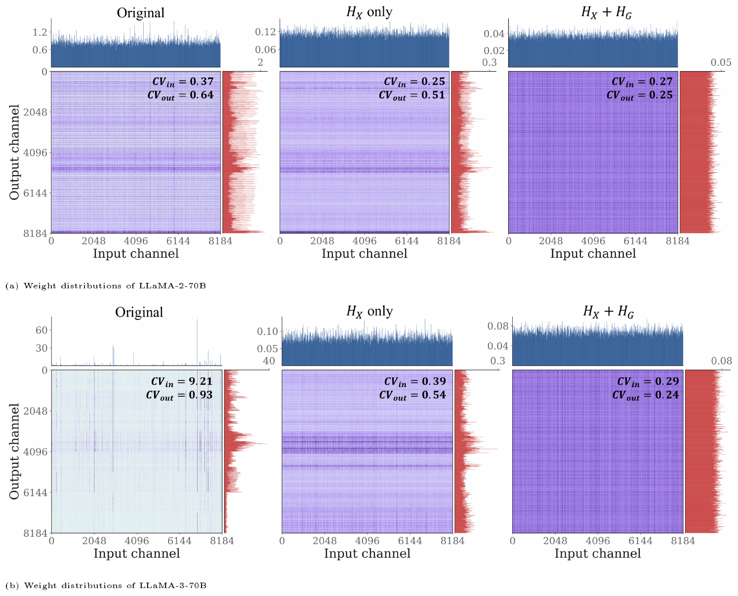
Figure 6 compares the weight magnitude distributions of LLaMA-3-70B and LLaMA-2-70B. In LLaMA-3-70B, the original weights exhibit extreme column-wise outliers ($\text{CV}\text{in} = 9.21$) concentrated on specific input dimensions, a phenomenon previously identified by [55] as unique to the LLaMA-3/3.1-70B family. These outliers expand the quantization range by orders of magnitude, causing the column-wise OBS updates in GPTQ and GPTAQ to produce degenerate solutions. In contrast, LLaMA-2-70B shows a substantially milder distribution ($\text{CV}\text{in} = 0.37$), consistent with its robustness to per-channel quantization. Applying $\mathbf{H}X$-only incoherence suppresses the input-side outliers in LLaMA-3-70B ($\text{CV}\text{in}: 9.21 \to 0.39$) but leaves the output-side heterogeneity largely unaddressed ($\text{CV}\text{out}: 0.93 \to 0.54$). BiIP further resolves the output-side structure via $\mathbf{H}G$, achieving $\text{CV}\text{in} = 0.29$ and $\text{CV}\text{out} = 0.24$, comparable to the post-BiIP values of LLaMA-2-70B ($0.27$ and $0.25$).

E. Per-Sublayer Calibration Memory

Table 22 details the memory required to perform calibration per sublayer for LLaMA-2-7B, LLaMA-3-8B, and LLaMA-2-13B, following the same convention as [12] (Table 9), with block slices of size $B=128$ included in all reported values. The Cholesky factor $\mathbf{L}$ is stored as a lower-triangular matrix and the correction matrix $\mathbf{P}$ as an upper-triangular matrix. $\textsc{KronQ}$ additionally stores $\mathbf{H}G$ as a full $d\mathrm{out} \times d_\mathrm{out}$ matrix during BiIP; once released, the remaining memory footprint is identical to GPTAQ. The peak memory overhead is therefore transient and confined to the BiIP preprocessing step.

::: {caption="Table 22: Memory needed to perform calibration (GiB) per sublayer. ^† $H_G$ released after BiIP, remaining memory matches GPTAQ."}

:::

F. Limitations

$\textsc{KronQ}$ requires a backward pass over the calibration set to estimate the gradient covariance $\mathbf{H}G$ prior to quantization, introducing additional offline computation relative to activation-only methods such as GPTQ and GPTAQ. Furthermore, $\mathbf{H}G$ is a full $d\mathrm{out} \times d\mathrm{out}$ matrix, incurring additional peak memory during BiIP preprocessing. Nevertheless, once $\mathbf{H}G$ is precomputed and stored, it incurs no additional computation during quantization itself, as $\mathbf{H}G$ cancels algebraically in the column-wise updates (Proposition 1) and is released upon completion of BiIP. During inference, $\textsc{KronQ}$ requires online reversion of the orthogonal transforms $\mathbf{U}$ and $\mathbf{V}$, introducing $\Theta(d{\mathrm{in}} \log d{\mathrm{in}} + d_{\mathrm{out}} \log d_{\mathrm{out}})$ overhead per layer. This is identical to QuIP# ([16]) and our fused CUDA kernel keeps the per-layer cost close to that of the $\Theta(d_{\mathrm{in}} d_{\mathrm{out}})$ weight matrix-vector multiply alone.

References

Section Summary: This references section compiles academic papers, preprints, and software tools centered on large language models such as the Llama series and GPT variants, along with methods for model compression. Many entries survey or propose techniques like quantization, which lowers numerical precision to speed up inference, and pruning, which removes less important parameters, often with a focus on post-training approaches that avoid full retraining. Additional citations cover related frameworks, memory optimizations, and evaluation benchmarks used in efficient AI deployment.

[1] Brown et al. (2020). Language models are few-shot learners. Advances in neural information processing systems. 33. pp. 1877–1901.

[2] Touvron et al. (2023). Llama: Open and efficient foundation language models. arXiv preprint arXiv:2302.13971.

[3] Grattafiori et al. (2024). The llama 3 herd of models. arXiv preprint arXiv:2407.21783.

[4] Gholami et al. (2022). A survey of quantization methods for efficient neural network inference.

[5] Liang et al. (2021). Pruning and quantization for deep neural network acceleration: A survey. Neurocomputing. 461. pp. 370–403.

[6] Zhao et al. (2025). Benchmarking post-training quantization in llms: Comprehensive taxonomy, unified evaluation, and comparative analysis. arXiv preprint arXiv:2502.13178.

[7] Hassibi, Babak and Stork, David (1992). Second order derivatives for network pruning: Optimal brain surgeon. Advances in neural information processing systems. 5.

[8] LeCun et al. (1989). Optimal brain damage. Advances in neural information processing systems. 2.

[9] Frantar, Elias and Alistarh, Dan (2022). Optimal brain compression: A framework for accurate post-training quantization and pruning. Advances in Neural Information Processing Systems. 35. pp. 4475–4488.

[10] Frantar et al. (2022). Gptq: Accurate post-training quantization for generative pre-trained transformers. arXiv preprint arXiv:2210.17323.

[11] Kim et al. (2024). Boa: Attention-aware post-training quantization without backpropagation. arXiv preprint arXiv:2406.13474.

[12] Li et al. (2025). Gptaq: Efficient finetuning-free quantization for asymmetric calibration. arXiv preprint arXiv:2504.02692.

[13] Tseng et al. (2025). Model-preserving adaptive rounding. arXiv preprint arXiv:2505.22988.

[14] Kim et al. (2025). GuidedQuant: Large language model quantization via exploiting end loss guidance. arXiv preprint arXiv:2505.07004.

[15] Chee et al. (2023). Quip: 2-bit quantization of large language models with guarantees. Advances in Neural Information Processing Systems. 36. pp. 4396–4429.

[16] Tseng et al. (2024). Quip#: Even better llm quantization with hadamard incoherence and lattice codebooks. Proceedings of machine learning research. 235. pp. 48630.

[17] Ashkboos et al. (2024). Quarot: Outlier-free 4-bit inference in rotated llms. Advances in Neural Information Processing Systems. 37. pp. 100213–100240.

[18] Liu et al. (2024). Spinquant: Llm quantization with learned rotations. arXiv preprint arXiv:2405.16406.

[19] Lin et al. (2024). Awq: Activation-aware weight quantization for on-device llm compression and acceleration. Proceedings of machine learning and systems. 6. pp. 87–100.

[20] Xiao et al. (2023). Smoothquant: Accurate and efficient post-training quantization for large language models. In International conference on machine learning. pp. 38087–38099.

[21] Thomas Wolf et al. (2020). Transformers: State-of-the-Art Natural Language Processing. In Proceedings of the 2020 Conference on Empirical Methods in Natural Language Processing: System Demonstrations. pp. 38–45. https://www.aclweb.org/anthology/2020.emnlp-demos.6.

[22] ModelCloud.ai and [email protected] (2024). GPT-QModel. https://github.com/modelcloud/gptqmodel. Contact: [email protected].

[23] Woosuk Kwon et al. (2023). Efficient Memory Management for Large Language Model Serving with PagedAttention. In Proceedings of the ACM SIGOPS 29th Symposium on Operating Systems Principles.

[24] Martens, James and Grosse, Roger (2015). Optimizing neural networks with kronecker-factored approximate curvature. In International conference on machine learning. pp. 2408–2417.

[25] Sun et al. (2024). Flatquant: Flatness matters for llm quantization. arXiv preprint arXiv:2410.09426.

[26] Hu et al. (2025). Ostquant: Refining large language model quantization with orthogonal and scaling transformations for better distribution fitting. arXiv preprint arXiv:2501.13987.

[27] Huang et al. (2024). SliM-LLM: Salience-driven mixed-precision quantization for large language models. arXiv preprint arXiv:2405.14917.

[28] Chen et al. (2024). Channel-wise mixed-precision quantization for large language models. arXiv preprint arXiv:2410.13056.

[29] Dong et al. (2020). Hawq-v2: Hessian aware trace-weighted quantization of neural networks. Advances in neural information processing systems. 33. pp. 18518–18529.

[30] Lee et al. (2025). Amq: Enabling automl for mixed-precision weight-only quantization of large language models. In Proceedings of the 2025 Conference on Empirical Methods in Natural Language Processing. pp. 35520–35538.

[31] Lee, Deokjae and Song, Hyun Oh (2026). Q-Palette: Fractional-Bit Quantizers Toward Optimal Bit Allocation for Efficient LLM Deployment. Advances in Neural Information Processing Systems. 38. pp. 11525–11558.

[32] Malinovskii et al. (2025). Higgs: Pushing the limits of large language model quantization via the linearity theorem. In Proceedings of the 2025 Conference of the Nations of the Americas Chapter of the Association for Computational Linguistics: Human Language Technologies (Volume 1: Long Papers). pp. 10857–10886.

[33] van der Ouderaa et al. (2023). The llm surgeon. arXiv preprint arXiv:2312.17244.

[34] Kunstner et al. (2019). Limitations of the empirical fisher approximation for natural gradient descent. Advances in neural information processing systems. 32.

[35] Botev et al. (2017). Practical Gauss-Newton optimisation for deep learning. In International Conference on Machine Learning. pp. 557–565.

[36] Merity et al. (2016). Pointer sentinel mixture models. arXiv preprint arXiv:1609.07843.

[37] Bisk et al. (2020). Piqa: Reasoning about physical commonsense in natural language. In Proceedings of the AAAI conference on artificial intelligence. pp. 7432–7439.

[38] Clark et al. (2018). Think you have solved question answering? try arc, the ai2 reasoning challenge. arXiv preprint arXiv:1803.05457.

[39] Zellers et al. (2019). Hellaswag: Can a machine really finish your sentence?. In Proceedings of the 57th annual meeting of the association for computational linguistics. pp. 4791–4800.

[40] Sakaguchi et al. (2021). Winogrande: An adversarial winograd schema challenge at scale. Communications of the ACM. 64(9). pp. 99–106.

[41] Clark et al. (2019). Boolq: Exploring the surprising difficulty of natural yes/no questions. In Proceedings of the 2019 conference of the north American chapter of the association for computational linguistics: Human language technologies, volume 1 (long and short papers). pp. 2924–2936.

[42] Mihaylov et al. (2018). Can a suit of armor conduct electricity? a new dataset for open book question answering. In Proceedings of the 2018 conference on empirical methods in natural language processing. pp. 2381–2391.

[43] Shao et al. (2023). Omniquant: Omnidirectionally calibrated quantization for large language models. arXiv preprint arXiv:2308.13137.

[44] Arai, Yamato and Ichikawa, Yuma (2025). Quantization error propagation: Revisiting layer-wise post-training quantization. arXiv preprint arXiv:2504.09629.

[45] Gemma Team (2025). Gemma 3 Technical Report. arXiv preprint arXiv:2503.19786.

[46] Guo et al. (2025). Deepseek-r1: Incentivizing reasoning capability in llms via reinforcement learning. arXiv preprint arXiv:2501.12948.

[47] Abouelenin et al. (2025). Phi-4-mini technical report: Compact yet powerful multimodal language models via mixture-of-loras. arXiv preprint arXiv:2503.01743.

[48] Rein et al. (2023). Gpqa: A graduate-level google-proof q&a benchmark. arXiv preprint arXiv:2311.12022.

[49] Hendrycks et al. (2020). Measuring massive multitask language understanding. arXiv preprint arXiv:2009.03300.

[50] Maxwell-Jia (2025). AIME 2024 Dataset. https://huggingface.co/datasets/Maxwell-Jia/AIME_2024. Hugging Face dataset.

[51] Jain et al. (2025). Livecodebench: Holistic and contamination free evaluation of large language models for code. In International Conference on Learning Representations. pp. 58791–58831.

[52] Jiang et al. (2024). Mistral 7B. arXiv 2023. arXiv preprint arXiv:2310.06825.

[53] Gao et al. (2024). The Language Model Evaluation Harness. doi:10.5281/zenodo.12608602. https://zenodo.org/records/12608602.

[54] Liu et al. (2025). Quantization hurts reasoning? an empirical study on quantized reasoning models. arXiv preprint arXiv:2504.04823.

[55] Qin, Minghai (2024). The uniqueness of llama3-70b series with per-channel quantization. arXiv preprint arXiv:2408.15301.