Train for the Worst, Plan for the Best: Understanding Token Ordering in Masked Diffusions

Jaeyeon Kim$^{*,1}$, Kulin Shah$^{*,2}$, Vasilis Kontonis$^{2}$, Sham Kakade$^{1}$, Sitan Chen$^{1}$

$^{1}$Harvard University

$^{2}$University of Texas Austin

$^{*}$Equal contribution

Correspondence to: Kulin Shah [email protected] Keywords: Machine Learning, ICML

In recent years, masked diffusion models (MDMs) have emerged as a promising alternative approach for generative modeling over discrete domains. Compared to autoregressive models (ARMs), MDMs trade off complexity at training time with flexibility at inference time. At training time, they must learn to solve an exponentially large number of infilling problems, but at inference time, they can decode tokens in essentially arbitrary order. In this work, we closely examine these two competing effects. On the training front, we theoretically and empirically demonstrate that MDMs indeed train on computationally intractable subproblems compared to their autoregressive counterparts. On the inference front, we show that a suitable strategy for adaptively choosing the token decoding order significantly enhances the capabilities of MDMs, allowing them to sidestep hard subproblems. On logic puzzles like Sudoku, we show that adaptive inference can boost solving accuracy in pretrained MDMs from $<7$ % to $\approx 90$ %, even outperforming ARMs with $7\times$ as many parameters and that were explicitly trained via teacher forcing to learn the right order of decoding. This shows that MDMs without knowledge of the correct token generation order during training and inference can outperform ARMs trained with knowledge of the correct token generation order. We also show the effectiveness of adaptive MDM inference on reasoning tasks such as coding and math on the 8B large language diffusion model (LLaDa 8B).

While diffusion models [1,2] are now the dominant approach for generative modeling in continuous domains like image, video, and audio, efforts to extend this methodology to discrete domains like text and proteins [3,4,5] remain nascent. Among numerous proposals, masked diffusion models (MDMs) [4,6,7] have emerged as a leading variant, distinguished by a simple and principled objective: to generate samples, learn to reverse a noise process which independently and randomly masks tokens.

In many applications, such as language modeling, masked diffusion models (MDMs) still underperform compared to autoregressive models (ARMs) [8,9], which instead learn to reverse a noise process that unmasks tokens sequentially from left to right. However, recent studies suggest that MDMs may offer advantages in areas where ARMs fall short, including reasoning [8,10], planning [11], and infilling [12]. This raises a key question: what are the strengths and limitations of MDMs compared to ARMs, and on what type of tasks can MDMs be scaled to challenge the dominance of ARMs in discrete generative modeling?

To understand these questions, we turn a microscope to two key competing factors when weighing the merits of MDMs over ARMs:

Therefore, we ask:

In this work, we provide dual perspectives on this question.

(1) Training for the worst. \enspace First, we provide theoretical and empirical evidence that the overhead imposed by training complexity quantifiably impacts MDMs' performance.

Theoretically, we show examples of simple data distributions with a natural left-to-right order, where ARMs can provably generate samples efficiently. In contrast, there are noise levels at which a large fraction of the corresponding subproblems solved by MDMs for these distributions are provably computationally intractable. Empirically, we validate this claim on real-world text data, known to have left-to-right order and show that the imbalance in training complexity across subproblems persists even in real-world text data (Figure 2, left).

While the above might appear to be bad news for MDMs, in the second part of this paper, we answer our guiding question in the affirmative by building upon the observation [13,14] that MDMs which can perfectly solve all masking subproblems can be used to decode in any order.

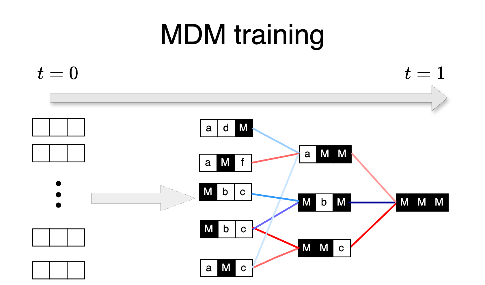
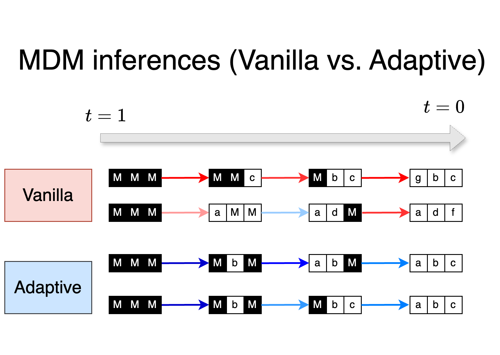
In first part of the paper, we show that the imbalance in complexity across subproblems during the training of MDMs results in some of the subproblems being poorly trained and the vanilla MDM inference that unmasks tokens in random order results in evaluating the poorly trained marginals. Therefore, in place of vanilla MDM inference, we consider adaptive strategies that carefully select which token to unmask next. Our key insight is that the adaptive strategies makes it possible to sidestep the hard subproblems from training (Figure 1). In particular, we find that even without modifying how MDMs are trained, the resulting models' logits contain enough information to determine the right order in which to unmask. We show the effectiveness of the adaptive inference in solving logic puzzles, coding, math and infilling tasks. For example, on Sudoku puzzles, a simple adaptive strategy (Section 4.1) improves the accuracy of MDMs from $<7$ % to almost 90%.

We show that the main effectiveness of MDMs lies in tasks that do not have the same natural token generation order across all sequences (e.g., logic puzzles and reasoning tasks like coding and math). By carefully designing experiments on logic puzzles, we show that MDMs without the knowledge of the correct token generation order during training and inference can outperform ARMs trained with the knowledge of the correct token generation order. In particular, we show that MDMs that decide the correct token generation order during inference via adaptive strategies can outperform ARMs that are trained to learn the right token generation order via supervised teacher forcing [15,16].

In Section 2, we provide preliminaries on MDMs and set notation. In Section 3, we examine MDM training and demonstrate the imbalance in computational intractability across subproblems. In Section 4, we consider adaptive inference in MDMs and investigate its impact on likelihood modeling across various tasks.

In this section, we explain the framework of Masked Diffusion Models [7,6] and highlight its interpretation as an order-agnostic learner. MDMs gradually add masking noise to the true discrete data and learn the marginal distribution of the induced reverse process. We formally define both the forward and reverse processes for MDMs below.

Let the distribution $p_{\rm{data}}$ on $\{1, \ldots, m\}^L$ be the data distribution over sequences of length $L$ and with vocabulary $\{1, \ldots, m\}$. We use $0$ to denote the "mask" token.

For a given $x_0 \sim p_{\rm{data}}$ and a noise level $t \in [0, 1]$, the forward process $x_t \sim q_{t|0}(\cdot \, | \, x_0)$ is a coordinate-independent masking process via $q_{t|0}(x_t | x_0) = \prod_{i=0}^{L-1} q_{t|0}(x_t^i | x_0^i)$, where

Here, $\alpha_t$ is a predefined noise schedule satisfying $\alpha_0 \approx 1, \alpha_1 \approx 0$ and $\mathbf{e}_{x_0^i} \in \mathbb{R}^{m+1}$ is a one-hot vector corresponding to the value of token $x_0^i$. $\mathrm{Cat}(\pi)$ denotes the categorical distribution given by $\pi \in \Delta^{m}$. In other words, for each $i$-th coordinate, $x_t^i$ is masked to the mask token $0$ with probability $1-\alpha_t$ and remains unchanged otherwise.

The reverse process of the above forward process is denoted by $q_{s|t}(x_s | x_t, x_0)$ and is given by $q_{s|t}(x_s | x_t, x_0) = \prod_{i=0}^{L-1} q_{s|t}(x_s^{i} | x_t, x_0)$ for any $s<t$, where

The reverse transition probability $q_{s|t}(x_s^i | x_t, x_0)$ is approximated using $g_{\theta}(x_s^i | x_t) \triangleq q_{s|t}(x_s^i \, \lvert\, x_t, x_0 \leftarrow p_{\theta}(\cdot | x_t, t))$ where $p_\theta(\cdot | x_t, t)$ is a denoising network trained to predict the marginal distribution on $x_0^i$ via an ELBO-based loss for all masked tokens at noise scale $t$ (i.e., for all $i$ such that $x_t^i = 0$). To be precise, $q_{s|t} \left(x_s^i \mid x_t, x_0 \leftarrow p_{\theta}(\cdot | x_t, t) \right)$ indicates the conditional probability where $p_{\theta}(\cdot | x_t, t)$ is placed in the position of $e_{x_0^i}$ within $q_{s|t}(x_s^i \mid x_t, x_0)$. The denoising network is trained to minimize the following loss derived from the score-entropy [4,6,7,17]:

where $\alpha_t'=\frac{d \alpha_t}{dt}$ and the summation is computed over masked tokens (i.e., all $i$ such that $x_t^i = 0$). In practice, a time-embedding-free architecture for the denoising network, i.e., $p_\theta(\cdot | x_t, t) = p_\theta(\cdot | x_t)$ is generally used as $x_t$ implicitly contains information about $t$ via the number of masked tokens.

The reverse sampling process starts from the fully masked sentence $x_1 = (0, \ldots, 0)$. Suppose we have a partially \fully masked sequence $x_t$ at a given noise level $t \in (0, 1]$ . Then, to obtain $x_s$ for a predetermined noise level $s < t$, we sample $x_s^i \sim g_\theta(\cdot | x_t)$ for all $i$. This process is repeated recursively from $t=1$ to $t=0$ .

In this section, we first discuss training of MDMs and compare it with ``left-to-right" order training of autoregressive models in Section 2.1.1. Then, we reformulate vanilla MDM inference in Section 2.1.2 to set the stage for the upcoming discussion.

Recent works [9,17] have observed that the learning problem of MDM is equivalent to a masked language model. Building upon their analysis, we reformulate the loss $\mathcal{L}_\theta$ to show that $\mathcal L_{\theta}$ is a linear combination of the loss for all possible infilling masks. We first define $x_0[M]$ as a masked sequence, obtained from original sequence $x_0$ where indices in the mask set $M$ (a subset of $[L]\triangleq\{1, 2, \ldots, L\}$) are replaced with mask token $0$.

Assume $\alpha_0=1$, $\alpha_1 =0$ and denoising network $p_\theta$ is time-embedding free.

Then $\mathcal{L}_\theta \le -\mathbb{E}_{x_0 \sim p_{\rm data}}[\log p_\theta(x_0)]$ and

where $|M|$ is the size of the set $M$ and $p_\theta(x_i \mid x_0[M])$ indicates the conditional probability of the $i$ -th coordinate from $p_\theta(x_t)$ .

The proof of the above proposition is given in Appendix E. As the MDM loss is a linear combination of the loss for all possible infilling mask $M$, the minimizer of the loss $\mathcal L_{\theta}$ learns to solve every masking problem. In other words, the optimal predictor $p_\theta$ is the posterior marginal of the $i$-th token, conditioned on $x_0[M]$ for all masks $M$.

On the other hand, Autoregressive Models (ARMs) learn to predict $i^{\textrm{th}}$ token $x^i$ based on all preceding tokens, from $x^0$ to $x^{i-1}$. This is equivalent to predicting $x^i$ by masking positions from $i$ to $L-1$. Therefore, the training objective for ARMs can be expressed as:

Typically, ARMs are trained to predict tokens sequentially from left to right. We refer to this as left-to-right training. However, it's also possible to train these models to predict tokens sequentially based on a fixed, known permutation of the sequence. We refer to this general approach as order-aware training.

To understand the comparison between the training objective of MDMs and ARMs, we want to highlight the equivalence between any-order autoregressive loss and MDM loss [18,17]. In particular, under conditions of Proposition 1, MDM loss is equal to

where $\textrm{Unif}(\mathbb S_L)$ is a uniform distribution over all the permutations of length $L$ (See Appendix E.1 for the proof). Observe that if the expectation is only with respect to the identity permutation, then the loss becomes an autoregressive loss. This shows that MDM loss solves exponentially more subproblems than ARM loss. In contrast to ARM loss, MDM does not prefer any particular (e.g., left-to-right) order during the training; therefore, we call its training order-agnostic training.

The MDM inference can be decomposed into two steps: (a) randomly selecting a set of positions to unmask and (b) assigning token values to each position via the denoising network $p_\theta$. More precisely, we can reformulate the reverse process $x_s \sim g_\theta(\cdot | x_t)$ as follows.

Therefore, the inference in MDM is implemented by randomly selecting $S$ and then filling each token value according to the posterior probability $p_{\theta}(x_s^i | x_t)$.

On the other hand, ARMs are trained to predict tokens sequentially from left to right and therefore, generate tokens also in left-to-right order. In contrast, vanilla MDM inference generates the tokens in a random order.

In this section, we provide theoretical and empirical evidence that when the data distribution has left-to-right order (or any fixed known order) then autoregressive training in left-to-right order (or in the known order) is more tractable than MDMs. In particular, for such distributions with fixed order, we show that ARMs can efficiently sample from the distributions but for MDMs, we theoretically and empirically demonstrate that a large portion of masking subproblems $p_\theta(x^i_0 \mid x_0[M])$ can be difficult to learn.

In Section 3.1, we show several examples of simple, non-pathological distributions for which: (1) the masking problems encountered during order-aware training (such as in ARMs) are computationally tractable, yet (2) many of the ones encountered during order-agnostic training (such as in MDMs) are computationally intractable. In Section 3.2, we empirically show that text data also exhibits this gap between the computational complexity of order-aware and order-agnostic training and therefore, MDMs train on subproblems of wide variety of complexity (depending on the order/masks). In Section 3.3, we empirically show that the variety in training complexity results in $\underline{\textbf{performance imbalance across subproblems}}$: MDMs trained on data from such distributions exhibits small errors on easy subproblems but suffers from large errors on harder ones.

We now describe a simple model of data under which we explore the computational complexity of masking problems and show the contrast between masking problems encountered by MDMs and ARMs.

A latents-and-observations (L&O) distribution is a data distribution $p_{\rm data}$ over sequence of length $L$ with alphabet size $m$ (precisely, $p_{\rm data}$ is over $\{0, \ldots, m\}^L$) is specified by a permutation $\pi$ over indices $\{1, 2, \ldots, L \}$, number of latent tokens $N$, number of observation tokens $P$ such that $N + P = L$, prior distribution $p_{\textrm{prior}}$ of latent variables over $\{1, \ldots, m\}$ and efficiently learnable observation functions $\mathcal{O}_1, \ldots, \mathcal{O}_P: \{1, \ldots, m\}^N \to \Delta(\{0, \ldots, m\})$, ¹

L&O distributions contain two types of tokens: (1) latent tokens and (2) observation tokens. Intuitively, latent tokens are tokens in the sequence, indexed by $\pi(1), \pi(2), \ldots, \pi(N)$ that serve as ``seeds" that provide randomness in the sequence; the remaining tokens, called observation tokens (indexed by $\pi(N+1), \pi(N+2), \ldots, \pi(N+P)$), are determined as (possibly randomized) functions of the latent tokens via $\mathcal{O}_1, \ldots, \mathcal{O}_P$. Observe that L&O distributions specified by a permutation $\pi$ have a natural generation order by permutation $\pi$.

Order-aware training, i.e. by permuting the sequence so that $\pi$ becomes the identity permutation and then performing autoregressive training, is computationally tractable: predicting $x^{\pi(i)}$ given $x^{\pi(1)}, \ldots, x^{\pi(i-1)}$ is trivial when $i \le N$ as the tokens are independent, and computationally tractable when $i > N$ because $x^{\pi(i)}$ only depends on $x^{\pi(1)}, \ldots, x^{\pi(N)}$ and is efficiently learnable by assumption. In contrast, below we will show examples where if one performs order-agnostic training à la MDMs, one will run into hard masking problems with high probability.

We first note that if the observations $(\mathcal{O}_1, \ldots, \mathcal{O}_P)$ are given by a cryptographic hash function, then the masking problem of predicting $(x^{\pi(1)}, \ldots, x^{\pi(L)})$ given $(x^{\pi(N+1)}, \ldots, x^{\pi(N+P)})$ is computationally intractable by design because it requires inverting the hash function. While this is a well-known folklore observation regarding the role of token ordering in language modeling, it is not entirely satisfying because this construction is worst-case in nature --- in real-world data, one rarely trains on sequences given by cryptographic hash functions. Furthermore, it only establishes hardness for a specific masking pattern which need not be encountered in the course of running the reverse process.

We provide several simple instances of L&O distributions that address these issues: instead of leveraging delicate cryptographic constructions, they are average-case in nature and furthermore we can establish hardness for typical masking problems encountered along the reverse process.

In all these examples, the hardness results we establish hold even if the algorithm knows all of the parameters of $p_{\rm data}$ as well as the observation functions $\mathcal{O}_1, \ldots, \mathcal{O}_P$. Due to space constraints, here we focus on the following example, deferring two others to Apps. Appendix B.1 and Appendix B.2.

Consider the following class of L&O distributions. Given arity $k\ge 2$, fix a predicate function $g: \{1, \ldots, m\}^k \to \{0, 1\}$. Consider the set of all ordered subsets of $\{1, 2, \ldots, N\}$ of size $k$ and set the total number of observation latents $P$ equal to the size of this set (hence $P = N ! / (N-k)! = N(N-1)\cdots(N-k+1)$). To sample a new sequence, we first sample latent tokens $x^{\pi(1)}, \ldots, x^{\pi(N)}$ from the prior distribution $p_{\textrm{prior}}$ and an observation latent corresponding to a $k$-sized subset $S$ is given by $g(\{ x^{\pi(i)} \}_{i \in S})$. In other words, each observation latent corresponds to a $k$-sized subset $S$ of $\{1, 2, \ldots, N\}$ and the corresponding observation function $\mathcal{O}_S(x^{\pi(1)}, \ldots, x^{\pi(N)})$ is given by $g(\{ x^{\pi(i)} \}_{i \in S})$.

Let $x$ be a sample from an L&O distribution $p_{\rm data}$ with sparse predicate observations as defined in Example 3, with arity $k$ and predicate $g$ satisfying Assumption 14, and let $\gamma$ be the probability that $g$ is satisfied by a random assignment from $\{1, \ldots, m\}^k$. Let $D_{\rm KS}$ and $D_{\rm cond}$ be some constants associated with the predicate function $g$ (see Definition 15). Suppose each token in $x$ is independently masked with probability $\alpha$, and $M$ is the set of indices for the masked tokens. If $1 - \gamma^{-1} D_{\rm KS}/kN^{k-1} \le \alpha \le 1 - \gamma^{-1} D_{\rm cond}/kN^{k-1}$, then under the 1RSB cavity prediction (see Conjecture 16), with probability $\Omega_k(1)$ over the randomness of the masking, no polynomial-time algorithm can solve the resulting subproblem of predicting any of the masked tokens among $x^{\pi(1)}, \ldots, x^{\pi(N)}$ given $x[M]$.

The complete proof of the proposition is given in Appendix B.4. We also provide a proof outline in Appendix B.3 for a comprehensive understanding.

In the previous section, we provided theoretical evidence that order-aware training is tractable when data has a natural order but the order-agnostic training is not. In this section, we provide empirical evidence to support this claim, using natural text data. Additionally, recent studies [8,9] have shown that masked diffusion models (MDMs) underperform compared to autoregressive models (ARMs) on natural text data. In this section, we provide evidence that this performance gap is primarily due to the order-agnostic training of MDMs. Natural text inherently follows a left-to-right token order, and we show that as training deviates from this order, model performance progressively declines.

To understand the importance of the order during the training, we use the following setting: Given a permutation $\pi$ of indices $\{0, 1, \ldots, L-1 \}$, define a * $\pi$-learner* to be a likelihood model $\log p_{\theta}(x_0)$ given as follows:

In other words, the $\pi$-learner predicts the token at position $\pi(i)$ given the clean tokens $x_0^{\pi(0)}, \ldots, x_0^{\pi(i-1)}$ and masked tokens $x_0^{\pi(i)}, \ldots, x_0^{\pi(L-1)}$. If $\pi$ is the identity permutation, this reduces to the standard (left-to-right) autoregressive training. Note that the MDM loss encodes a $\pi$-learner for every permutation $\pi$ because the MDM loss Equation 1 is equivalent to the average loss of those $\pi$-learners over $\pi$ sampled from $\mathrm{Unif}(\mathbb{S}_L)$:

where $\mathbb{S}_L$ denotes the set of all permutations over $\{0, 1, \ldots, L-1\}$. The proof of the above equivalence is given in Appendix E. Therefore, by measuring the 'hardness' of each $\pi$-learner, we can probe differences in hardness between arbitrary masking problems and left-to-right masking problems.

We use the Slimpajama dataset [19] to evaluate the performance of training in different orders. To train a $\pi$-learner, we employ a transformer with causal attention and use permuted data $\pi(x_0)$ as input. By varying $\pi$ while maintaining all other training configurations (e.g., model, optimization), we can use the resulting likelihood (computed using Equation 3) as a metric to capture the hardness of subproblems solved by the $\pi$-learner.

In our experiments, the sequence length $L$ is $2048$, so repeating the scaling laws for each $\pi$ is infeasible. Instead, we sample $\pi \sim \mathrm{Unif}(\mathbb{S}_L)$ and examine the scaling law of the $\pi$-learner's likelihood. We leverage the codebase from [8], where the baseline scaling laws of MDM and ARM were introduced. Moreover, given that RoPE has an inductive bias towards left-to-right ordering, we employ a learnable positional embedding layer for all experiments to correct this. Consequently, we also re-run the baseline results, where RoPE was employed. To investigate how the distance between $\pi$ and the identity permutation affects the scaling law, we consider two interpolating distributions over permutations between $\mathrm{Unif}(\mathbb{S}_L)$ (i.e, MDM training) and the point mass at the identical permutation (i.e, ARM training). We sample three permutations from the interpolating distribution and $\mathrm{Unif}(\mathbb{S}_L)$ and plot the scaling law for each of the permutation. Due to space constraints, we provide further experimental details in Appendix C.1.

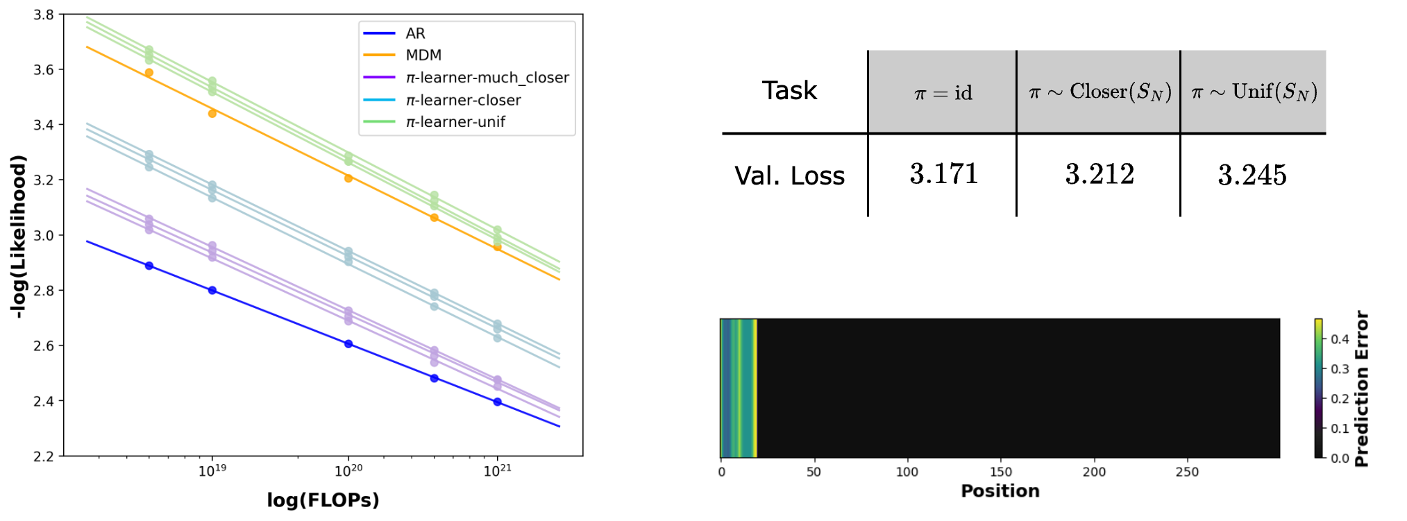
As shown in Figure 2, the scaling law for a $\pi$-learner with uniformly random $\pi$ is worse than that of an ARM. This elucidates the inherent hardness of masking problems $p_\theta(x_i \mid x_0[M])$ beyond left-to-right prediction and also explains why MDM, which is trained simultaneously on all $\pi \in \mathbb{S}_L$, is worse than ARM in likelihood modeling. Additionally, as $\pi$ gets closer to the identity permutation, the scaling laws also get closer to ARM ($\pi$-learner-closer and $\pi$-learner-much-closer in Figure 2). This also supports the common belief that ARM is a good fit for text data as it inherently follows a left-to-right ordering.

That said, it should also be noted that even though MDMs are trained on exponentially more masking problems than ARM ($\Theta(L2^L)$ versus $L$), its performance is not significantly worse than $\pi$-learners. We attribute this to the blessing of task diversity; multi-task training can benefit both the optimization dynamics [20] and validation performance [21,22,23] due to positive transfers across tasks.

In previous sections, we have demonstrated that the hardness of different masking problems $p_\theta(x^i \mid x_0[M])$ can vary significantly, potentially hindering the MDM's learning. In this section, we provide empirical evidence that the MDM's final performance exhibits a similar imbalance across subproblems. Details are provided in App. Appendix C.2.

Consider an L&O distribution with $\pi$ given by the identity permutation and where each observation $\mathcal{O}_j$ is deterministically given by $\mathrm{NAE}(x_{i_1}, x_{i_2}, x_{i_3}) \triangleq 1 - \mathbf{1}[x_{i_1} = x_{i_2} = x_{i_3}]$ for some randomly chosen (prefixed) triples $(i_1, i_2, i_3) \in[N]$. For an MDM trained on this distribution, we measure the error it achieves on each task $\log p_\theta(x_0 | x_0[M])$ via $\mathbb{E}_{x_0} \Bigl \| \log p_\theta(x_0 | x_0[M])- \log p_{\rm data}(x_0 | x_0[M]) \Bigr\|^2$, where $p_{\rm data}(x_0 | x_0[M])$ denotes the Bayes-optimal predictor. Technically, we do not have access to this, so instead we train another MDM for a much larger number of iterations and use this as a proxy. Figure 2 reveals that prediction tasks for latent positions (light region) exhibit larger errors compared to those for observation positions (dark region).

Here we revisit the text experiment from Section 3.2. Since we do not have access to the Bayes-optimal predictor, we use the metric $\mathbb{E}_{x_0 \sim p_{\rm{data}}}\left[\sum_{i=0}^{L-1} \log p_\theta \left(x_0^{\pi(i)} \Big| x_0 [\pi\{i, \ldots, L-1\}] \right) \right]$. This captures the accumulation of error across subproblems $p_\theta \left(x_0^{\pi(i)} \Big| x_0 [\pi\{i, \ldots, L-1\}] \right)$, since $p_\theta(x_0 | x_0[M]) = p_{\rm{data}}(x_0 | x_0[M])$ minimizes this metric. Figure 2 shows a clear gap between different subproblems.

The theoretical and empirical evidence demonstrates that MDMs perform better in estimating $p_{\theta}(x_0 | x_0[M])$ for some subproblems $M$ than for others. We therefore want to avoid encountering hard subproblems $M$ at inference time. In the next section, we show that while vanilla MDM inference can run into such subproblems, simple modifications at the inference stage can effectively circumvent these issues, resulting in dramatic, training-free performance improvements.

We previously argued that due to the complex nature of masking subproblems, MDM must perform poorly on certain ones $p_\theta(x^i | x_t)$. Therefore, during vanilla MDM inference, MDM inevitably encounters such difficult subproblems at Step (b). While this might suggest that we need to fundamentally revisit how MDMs are trained, in this section we show that, surprisingly, simple modifications at the inference stage—without any further training—can sidestep these issues and lead to significant performance improvements.

The vanilla MDM inference (Algorithm 1) aim to align the intermediate distributions with the forward process, as used in continuous diffusion. However, unlike continuous diffusion, the reverse process of MDM allows multiple valid sampling paths (different orders of unmasking the tokens) that match the starting distribution of the forward process of MDM.

We first show that when we have an ideal MDM that perfectly solves all masking problems, i.e., $p_\theta(x_0^i | x_0[M]) = p_{\rm{data}}(x_0^i | x_0[M])$, then using any sampling path (unmasking the tokens in any order) results in the same distribution. Consider the following sampler: For every step, $S$ is a set with one index selected agnostically (without following any distribution). For any clean sample $x_0$ generated by this sampler, note that $p_\theta(x_0) = \prod_{i=0}^{L-1} p_\theta \left(x_0^{\pi(i)} \Big| x_0 [\pi\{i, \ldots, L-1\}] \right)$ by chain rule, and this is equal to $\prod_{i=0}^{L-1} p_{\rm{data}} \left(x_0^{\pi(i)} \Big| x_0 [\pi\{i, \ldots, L-1\}] \right) = p_{\rm{data}}(x_0)$. Therefore, other choices of $S$, not necessarily following Algorithm 1, still capture the true likelihood.

In practice, unlike this ideal case, MDM does not perform equally well on all subproblems, as shown in Section 3.3. Consequently, different sampling paths result in varying likelihood modeling abilities. Motivated by this observation, we consider adaptive inference for MDMs:

Instead of selecting $S$ randomly, adaptive MDM inference leverages an oracle $\mathcal{F}(\theta, x_t)$ to select $S$ strategically to avoid hard masking problems. This naturally raises the question of how to design an effective oracle $\mathcal{F}$.

In the following sections, we demonstrate that adaptive MDM inference with careful choices of $\mathcal{F}$ enhance MDM's likelihood matching ability. In other words, a pretrained MDM, even if it performs poorly on certain hard subproblems, still contains sufficient information to avoid them when paired with an effective oracle $\mathcal{F}$.

We introduce two different oracles, Top probability and Top probability margin. Intuitively, both strategies are based on the idea that $S$ should be selected based on how "certain" the model is about each position. We caution that these strategies should not be confused with notions like nucleus sampling in ARMs [25]; the oracles we describe are for selecting the position of the next token to decode, rather than the value, and thus are only meaningful in the context of MDMs.

Suppose we want to unmask $K$ positions at time step $t$, i.e., select $|S|=K$. In the top probability, the uncertainty of a position is estimated by the maximum probability assigned to any value in the vocabulary. More precisely, the certainty at position $i$ is $\max_{j \in \{ 0, \ldots, m-1 \} } p_\theta(x^i = j | x_t)$ and $\mathcal{F}(\theta, x_t) = \text{Top } K \left(\max p_\theta(x^i | x_t) \right)$ .

Top probability strategy is a good proxy for many tasks and works well in practice [14,11,26]. However, this approach can often provide misleading estimates of uncertainty. Consider when an MDM is confused between two token values, thus assigning them almost equal but high probabilities. In this case, unmasking according to top probability may still choose to unmask this position, despite its uncertainty. To mitigate this issue, we propose the following alternative strategy.

In this strategy, the uncertainty of a position is instead estimated using the absolute difference between the two most probable values at position $i$. More precisely, if $j_1$ and $j_2$ are the two most probable values in vocabulary according to $p_\theta(x^i | x_t)$ in position $i$, the certainty in the position is given by $| p_\theta(x^i = j_1 | x_t) - p_\theta(x^i = j_2 | x_t) |$ and $\mathcal{F}(\theta, x_t) = \text{Top } K \left(| p_\theta(x^i = j_1 | x_t) - p_\theta(x^i = j_2 | x_t) | \right)$ . When multiple values have similar probabilities at a position, top probability margin strategy will provide a better estimate of the uncertainty of a position, and when there is a single best choice of value then top probability and top probability margin work similarly.

In this section, we experimentally validate that adaptive MDM inference helps MDMs avoid hard subproblems, leading to better likelihood matching. We first show our results on L&O-NAE-SAT and text data, before turning to our primary application to logic puzzles.

L&O-NAE-SAT and text data. For the L&O-NAE-SAT distribution defined in Section 3.3, we evaluate the effectiveness of adaptive inference by measuring the accuracy in predicting the observation tokens. Table 1 in the appendix reveals a clear improvement over vanilla inference. For the text dataset, we evaluate using the standard metric of generative perplexity, by which likelihood is measured by a large language model. We also compute the entropy of the generated samples to ensure both inference strategies exhibit similar levels of diversity. As shown in Figure 3, we observe a substantial decrease in generative perplexity using adaptive inference. We defer further experimental details to Appendix D.1.

Logic puzzles. We consider two different types of logic puzzles: Sudoku and Zebra (Einstein) puzzles. Intuitively, for Sudoku, some empty (masked) cells are significantly easier to predict than others and we want to choose the cells that are easier to predict during the inference. We evaluate the effectiveness of adaptive MDM inference over vanilla MDM inference in selecting such cells.²

To measure the performance of an inference method, we use the percentage of correctly solved puzzles. For both puzzles, we use train and test datasets from [15]. For the Sudoku puzzle (Table 2) we observe that adaptive MDM inference, in particular, Top probability margin strategy, obtains substantially higher accuracy (89.49%) compared to vanilla MDM inference (6.88%). Additionally, Top probability margin obtains higher accuracy (89.49%) than Top probability strategy (18.51%). As mentioned in Section 4.1, this is because Top probability margin strategy more reliably estimates uncertainty when multiple competing values are close in probability at a given position, as is often the case in Sudoku. For the Zebra puzzle, as shown in Table 3, we observe a consistent result: Top probability (98.5%) and Top probability margin (98.3%) outperform vanilla MDM inference (76.9%).

In this section, we study the effectiveness of adaptive MDM inference in finding the right reasoning/generation order for tasks where every sequence has a different "natural" order. To do so, we will compare the performance of adaptive MDM inference to that of ARM on Sudoku and Zebra puzzles. For these puzzles, the natural order of generation is not only different from left-to-right, but it is also sequence-dependent. For such tasks, prior works have shown that ARMs struggle if the information about the order is not provided during the training [15,16]. Therefore, to obtain a strong baseline, we not only consider an ARM trained without the order information but also consider an ARM trained with the order information for each sequence in the training data. Note that the latter is a much stronger baseline than the former as one can hope to teach the model to figure out the correct order by some form of supervised teacher forcing (as performed in [15,16]), eliminating the issue of finding the right order in an unsupervised manner.

We compare ARMs and MDMs for Sudoku in Table 2 and Zebra puzzles in Table 3. We observe that for both, Top probability margin-based adaptive MDM inference not only outperforms the ARM trained without ordering information, but it even outperforms the ARM trained with ordering information! This shows that the unsupervised way of finding the correct order and solving such logic puzzles using adaptive MDM inference outperforms the supervised way of finding the correct order and solving such puzzles using an ARM, and is significantly less computationally intensive.

To examine the effect of different inference strategies on text benchmarks, we adapted LLaDA, the 8B MDM model from [27]. We compare three inference strategies: vanilla, top probability, and top probability margin. The results are presented in Table 4.

We see that both adaptive MDM inference strategies, top probability and top probability margin, consistently outperform vanilla MDM inference. Notably, top probability margin demonstrates a clear advantage over top probability in challenging tasks like HumanEval-Multiline (infill), HumanEval-Split Line (infill), and Math. This is because Top probability margin provides a more reliable estimate of uncertainty when multiple tokens have similar probabilities, a frequent occurrence in these difficult tasks. These results further underscore the potential for developing new, sophisticated adaptive inference strategies for various tasks. We provide experimental details in Appendix D.3.

In the previous section we showed that when the training and inference sequences come from the same distribution, order-agnostic training of MDMs combined with adaptive inference can perform very well on logic puzzles. To evaluate if the model has learned the correct way of solving the puzzles and test the robustness of adaptive inference, we also test the MDMs on harder puzzles than the ones from training, for Sudoku.

We keep the training dataset the same as proposed in [15]. [15] created this dataset from [28] by selecting the puzzles that can be solved using 7 fixed strategies and do not require backtracking-based search. We use the remaining puzzles in [28] as our hard dataset. Hence, these puzzles all use a strategy not seen during training and/or backtracking to obtain the correct solution.

We measure the accuracy of MDMs and ARMs on the hard test set and present the results in Table 5. We see that the Top probability margin-based adaptive MDM inference strategy (49.88%) again significantly outperforms ARMs trained with order information (32.57%). In particular, although the accuracy drops for both methods due to the more challenging test set, MDMs with adaptive inference appear to be more robust to this distribution shift than ARMs. We believe this is due to the fact that MDMs try to solve a significantly higher number of infilling problems than ARMs ($\exp(L)$ compared to $L$) and therefore are able to extract knowledge about the problem more efficiently than ARMs.

In this work, we examined the impact of token generation order on training and inference in MDMs. We provided theoretical and experimental evidence that MDMs train on hard masking problems. We also demonstrated that adaptive inference strategies can be used to sidestep these hard problems. For logic puzzles, we find that this leads to dramatic improvements in performance not just over vanilla MDMs, but even over ARMs trained with teacher forcing to learn the right order of decoding. An important direction for future work is to go beyond the relatively simple adaptive strategies to find a better generation order like top probability and top probability margin considered here.

JK thanks Kiwhan Song for discussions about MDM training. KS and VK are supported by the NSF AI Institute for Foundations of Machine Learning (IFML). KS and VK thank the computing support on the Vista GPU Cluster through the Center for Generative AI (CGAI) and the Texas Advanced Computing Center (TACC) at UT Austin. KS thanks Nishanth Dikkala for the initial discussions about the project. SK acknowledges: this work has been made possible in part by a gift from the Chan Zuckerberg Initiative Foundation to establish the Kempner Institute for the Study of Natural and Artificial Intelligence and support from the Office of Naval Research under award N00014-22-1-2377. SC is supported by the Harvard Dean's Competitive Fund for Promising Scholarship and thanks Brice Huang and Sidhanth Mohanty for enlightening discussions about computational-statistical tradeoffs for planted CSPs.

This paper advances the understanding of discrete diffusion models, contributing to the broader field of Machine Learning. There are many potential societal consequences of our work, none of which we feel must be specifically highlighted here.

(Continuous) diffusion models were originally built on continuous-space Markov chains with Gaussian transition kernels [29,1]. This was later extended to continuous time through the theory of stochastic differential equations [2]. In a similar vein, discrete diffusion models have emerged from discrete-space Markov chains [5]. Specifically, [3] introduced D3PM with various types of transition matrices. Later, [4] proposed SEDD, incorporating a theoretically and practically robust score-entropy objective. Additionally, [30,31] introduced novel modeling strategies that classify tokens in a noisy sequence as either signal (coming from clean data) or noise (arising from the forward process). In particular, [31] uses this to give a planner that adaptively determines which tokens to denoise. While this is similar in spirit to our general discussion about devising adaptive inference strategies, we emphasize that their approach is specific to discrete diffusions for which the forward process scrambles the token values, rather than masking them.

Meanwhile, the absorbing transition kernel has gained popularity as a common choice due to its better performance than other kernels. Building on this, [6,7] aligned its framework with continuous diffusion, resulting in a simple and principled training recipe, referring to it as Masked Diffusion Model. Subsequent studies have explored various aspects of MDM. [12] efficiently trained MDM via adaptation from autoregressive models, scaling MDM up to 7B parameters. [9] interpreted MDMs as order-agnostic learners and proposed a first-hitting sampler based on this insight. [11,12] demonstrated that MDM outperforms autoregressive models in reasoning and planning tasks, emphasizing its impact on downstream applications. [8] examined the scaling laws of MDM, while [32,33] identified limitations in capturing coordinate dependencies when the number of sampling steps is small and proposed additional modeling strategies to address this issue. [34] studied conditional generation using MDM and [35] tackled the challenge of controlling generated data distributions through steering methodologies. [36] provided a theoretical analysis showing that sampling error is small given accurate score function estimation.

Even though language tasks generally have a natural order of left-to-right" token generation, in many tasks like planning, reasoning, and combinatorial optimization, the natural order of token generation can be quite different from left-to-right". Even though prominent autoregressive-based language models achieve impressive performance on various tasks, many works [37,38,10] have shown that this performance is tied to the training order of the tasks and therefore can cause brittleness from it. For example, [38] showed that simply permuting the premise order on math tasks causes a performance drop of 30%. The reason behind such brittleness regarding the ordering is the inherent ``left-to-right" nature of the autoregressive models. Several works [39] have tried to address this issue in the autoregressive framework. In particular, [40] highlighted the significance of left-to-right ordering in natural language by comparing its likelihood to that of the reverse (right-to-left) ordering.

Recently, discrete diffusion models have emerged as a promising approach for discrete data apart from autoregressive models. Additionally, the order-agnostic training of discrete diffusion models opens up the multiple sampling paths during the inference but it also faces some challenges during the training therefore, they seem a promising approach to elicit any order reasoning. [14] proposed different ways of implementing an adaptive inference strategy for MDM but a concrete understanding of why such an adaptive inference strategy is needed is still lacking. In this work, we explore various aspects of vanilla MDM training and how adaptive MDM inference can mitigate the issues raised by vanilla MDM training and elicit any order reasoning.

We also want to mention the concurrent work by [41] that proposes an alternative adaptive inference strategy by selecting $\mathcal F(\theta, x_t)$ based on the BERT model or the denoiser itself. In particular, [41] uses the BERT model or the denoiser to obtain the uncertainty of a token and then uses Top- $K$ to decide the positions to unmask it. In contrast to their work, we disentangle the impact of token ordering on MDM training vs. MDM inference and provide a more complete understanding of the motivations for and benefits of adaptive inference. Additionally, our results indicate drawbacks to using Top- $K$ strategy as opposed to Top- $K$ margin in deciding which tokens to unmask when there are multiple values with high probabilities.

Efforts to learn the natural language using non-autoregressive modeling began with BERT [42]. Non-causal approaches can take advantage of the understanding the text data representation. [13] adopted a similar approach for learning image representations. Building on these intuitions, [43,18] proposed any-order modeling, which allows a model to generate in any desired order. [43] made the same observation that any-order models by default have to solve exponentially more masking problems than autoregressive models. However, whereas our work shows that learning in the face of this challenging task diversity can benefit the model at inference time, their work sought to alleviate complexity at training time by reducing the number of masking problems that need to be solved.

Throughout this section, we use $x^i$ to denote the $i$-th coordinate of the vector $x$ and $z{(j)}$ to denote the $j$-th example. The $i$-th coordinate of the vector $z{(j)}$ is denoted by $z{(j)}^i$.

Let $m = 2$, $k\in\mathbb{N}$, and $N^2\log N \ll P \le N^{0.49k}$. Fix noise rate $\eta > 0$ as well as strings $z{(1)}, \ldots, z{(P)}$ sampled independently and uniformly at random from the set of $k$-sparse strings in $\{0, 1\}^N$. For each $j\in[P]$, define $\mathcal{O}_j(x)$ to be the distribution which places mass $1 -\eta$ on $1$ (resp. $2$) and mass $\eta$ on $2$ (resp. $1$) if $\sum_i x^i z{(j)}^i$ is odd (resp. even). Note that for $k = O(1)$, each of these observations is efficiently learnable by brute-force.

Below we show that for a certain range of masking fractions, a constant fraction of the masking problems for the corresponding L&O distributions are computationally hard under the Sparse Learning Parity with Noise assumption [44]. Formally we have:

Let $0 < \alpha < 1$ be an arbitrary absolute constant, and let $\eta = 1/\mathrm{poly}(N)$ be sufficiently large. Let $x$ be a sample from a L&O distribution $p_{\rm data}$ with noisy parity observations as defined in Example 5. Suppose each token is independently masked with probability $\alpha$, and $M$ is the set of indices for the masked tokens. If $1 - 1/N \le \alpha \le 1 - 1/2N$, then under the Sparse Learning Parity with Noise (SLPN) assumption (see Definition 7), with constant probability over $M$, no polynomial-time algorithm can solve the resulting masking problem of predicting any of the masked tokens among $x^{\pi(1)}, \ldots, x^{\pi(N)}$ given $x[M]$.

We note that it is important for us to take the observations to be sparse parities and to leverage the Sparse Learning Parity with Noise assumption. If instead we used dense parities and invoked the standard Learning Parity with Noise (LPN) assumption, we would still get the hardness of masking problems, but the observations themselves would be hard to learn, assuming LPN. This result is based on the following standard hardness assumption:

Given input dimension $N$, noise parameter $0 < \eta < 1/2$, and sample size $P$, an instance of the Sparse Learning Parity with Noise (SLPN) problem is generated as follows:

Given the examples $\{(x{(i)}, y{(i)})\}^P_{i=1}$, the goal is to recover $x$.

The SLPN assumption is that for any $P = N^{(1 - \rho)k/2}$ for constant $0 < \rho < 1$, and any sufficiently large inverse polynomial noise rate $\eta$, no $\mathrm{poly}(N)$-time algorithm can recover $x$ with high probability.

Proof of Proposition 6: With probability at least $1 - (1 - 1/N)^N \ge \Omega(1)$, all of the variable tokens $x^{\pi(i)}$ for $i \le N$ are masked. Independently, the number of unmasked tokens among the observation tokens $\mathcal{O}_j$ is distributed as $\mathrm{Bin}(P, 1-\alpha)$, so by a Chernoff bound, with probability at least $1 - e^{-\Omega(P/N^2)} = 1 - 1/\mathrm{poly}(N)$ we have that at least $P/4N = \Omega(N\log N)$ observation tokens are unmasked. The masking problem in this case amounts to an instance of SLPN with input dimension $N$ and sample size in $[\Omega(N\log N), O(N^{0.49k})]$. Because of the lower bound on the sample size, prediction of $\mathbf{x}^M$ is information-theoretically possible. Because of the upper bound on the sample size, the SLPN assumption makes it computationally hard. As a result, estimating the posterior mean on any entry of $\mathbf{x}^M$ given the unmasked tokens is computationally hard as claimed.

Let $m = 2$ and $P = \gamma N^2$ for constant $\gamma > 0$. Fix slab width $\beta$ and vectors $z{(1)}, \ldots, z{(P)}$ sampled independently from $\mathcal{N}(0, I)$. For each $j\in[P]$, define the corresponding observation $\mathcal{O}_j(x)$ to be deterministically $1$ if $|\langle z{(j)}, 2x - \mathbf{1}\rangle| \le \beta\sqrt{N}$, and deterministically $0$ otherwise.

In [45], it was shown that stable algorithms (Definition 10), which encompass many powerful methods for statistical inference like low-degree polynomial estimators, MCMC, and algorithmic stochastic localization [46], are unable to sample from the posterior distribution over a random bitstring conditioned on it satisfying $|\langle z{(j)}, x\rangle| \le \beta\sqrt{N}$ for any $\Theta(N)$ number of constraints $z{(1)}, \ldots, z{(P')}$, provided $P'$ is not too large that the support of the posterior is empty. This ensemble is the well-studied symmetric perceptron [47]. The following is a direct reinterpretation of the result of [45]:

Let $p_{\rm data}$ be a L&O distribution with random slab observations as defined in Example 8, with parameter $\gamma > 0$ and slab width $\beta > 0$. There exists a constant $c_\beta > 0$ such that for any absolute constant $0 < c < c_\beta$, if $1 - c_\beta N/2P \le \alpha \le 1 - c N / P$ and $\gamma > c_\beta$, the following holds. Let $p'_{\rm data}$ denote the distribution given by independently masking every coordinate in $p_{\rm data}$ with probability $\alpha$. Then any $(1 - \tilde{\Omega}(1/\sqrt{N}))$-stable algorithm, even one not based on masked diffusion, which takes as input a sample $x'$ from $p'_{\rm data}$ and, with probability $1 - o(1)$ outputs a Wasserstein-approximate³ sample from $p_{\rm data}$ conditioned on the unmasked tokens in $x'$, must run in super-polynomial time.

The upshot of this is that any stable, polynomial-time masked diffusion sampler will, with non-negligible probability, encounter a computationally hard masking problem at some point during the reverse process.

For the proof, we first formally define the (planted) symmetric Ising perceptron model:

Let $\alpha, \beta > 0$. The planted symmetric Ising perceptron model is defined as follows:

The goal is to sample from the posterior on $\sigma$ conditioned on these observations $\{z{(i)}\}^P_{i=1}$.

Next, we formalize the notion of stable algorithms.

Given a matrix $Z\sim\mathcal{N}(0, 1)^{\otimes P\times N}$, define $Z_t = tZ + \sqrt{1 - t^2}Z'$ for independent $Z'\sim\mathcal{N}(0, 1)^{\otimes P\times N}$.

A randomized algorithm $\mathcal{A}$ which takes as input $Z\in\mathbb{R}^{P\times N}$ and outputs an element of $\{\pm 1\}^N$ is said to be * $t_N$-stable* if $\lim_{N\to\infty} W_2(\mathrm{law}(\mathcal{A}(Z)), \mathrm{law}(\mathcal{A}(Z_t))) = 0$.

As discussed at depth in [46], many algorithms like low-degree polynomial estimators and Langevin dynamics are stable.

For any constant $\beta > 0$, there exists $c_\beta > 0$ such that the following holds for all constants $0 < \alpha < c_\beta$. For $t_N \le 1 - \Omega(\log^2(n) / n^2)$, any $t_N$-stable randomized algorithm $\mathcal{A}$ which takes as input $Z = (z{(1)}, \ldots, z{(P)})$ and outputs an element of $\{\pm 1\}^N$ will fail to sample from the posterior on $\sigma$ conditioned on $Z$ in the symmetric Ising perceptron model to Wasserstein error $o(\sqrt{N})$.

Proof of Proposition 9: By a union bound, with probability at least $1 - (1 - \alpha) N \ge 1 - c_\beta N^2/P \ge 1 - c_\beta /\gamma$ over a draw $x' \sim p'_{\rm data}$, all of the $x^{\pi(i)}$ tokens are masked. The number of unmasked tokens in $x'$ among the observations $\mathcal{O}_j$ is distributed as $\mathrm{Bin}(P, 1 - \alpha)$. By a Chernoff bound, this is in $[3cN/4, 3c_\beta N/4]$ with at least constant probability. The claim then follows immediately from Theorem 11 above.

To understand the proof idea, we consider the case where all the latent tokens are masked and some of the observation tokens are unmasked. In this case, the prediction task reduces to learning to recover the latent tokens that are consistent with the observations. Intuitively, each observation provides some constraints and the task is to recover an assignment that satisfies the constraints. This is reminiscent of Constraint Satisfaction Problems (CSPs). Indeed, to show the hardness result, we use the rich theory developed for planted CSPs at the intersection of statistical physics and average-case complexity.

In a planted CSP, there is an unknown randomly sampled vector $y$ of length $N$ and, one is given randomly chosen Boolean constraints which $y$ is promised to satisfy, and the goal is to recover $y$ as best as possible (see Definition 12). Prior works have shown the hardness of efficiently learning to solve the planted CSP problem [48,45]. We show the hardness of masking problems in L&O distributions based on these results. Consider the ground truth latent tokens as the random vector $y$ and each observation as a constraint. In this case, the problem of learning to recover the latent tokens from the observation tokens reduces to recovery for the planted CSP.

There are precise predictions for the values of vocabulary size $m$ and the number of observations for which the information-theoretically best possible overlap and the best overlap achievable by any computationally efficient algorithm are different. We show that these predictions directly translate to predictions about when masking problems become computationally intractable:

As a simple example, let us consider sparse predicate observations with $k=2$ and $g(x', x'') = \mathbf{1}[x' \neq x'']$. These can be formally related to the well-studied problem of planted $m$-coloring. In the planted $m$-coloring, a random graph of average degree $D$ is sampled consistent with an unknown vertex coloring and the goal is to estimate the coloring as well as possible [48], as measured by the overlap of the output of the algorithm to the ground-truth coloring (see Definition 12). As a corollary of our main result, we show that when all the latent tokens $x^{\pi(1)}, \ldots, x^{\pi(N)}$ are masked and a few unmasked observation tokens provide the information of the form $g(x^{\pi(i)}, x^{\pi(j)}) = \mathbf{1}[x^{\pi(i)} \neq x^{\pi(j)}]$ for $i, j \leq N$, then solving the masking problem can be reduced to solving planted coloring.

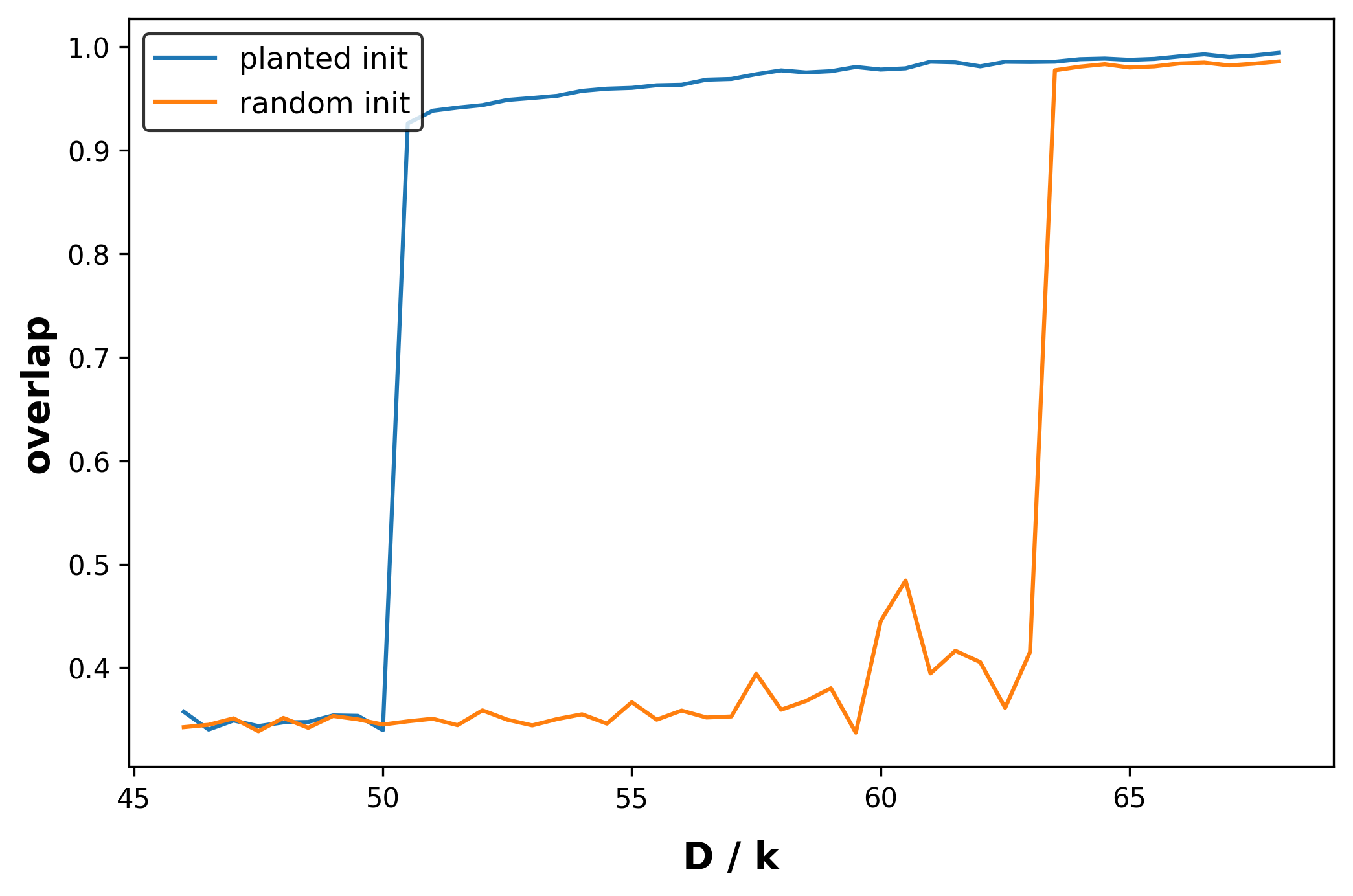
For planted $m$-coloring, when $m = 5$ the thresholds in Proposition 4 are given by $D_{\rm KS} / 2 = 16$ and $D_{\rm cond} / 2 \approx 13.23$ [48] (the factor of $2$ here is simply because the observations correspond to ordered subsets of size $2$). For general predicates and arities, there is an established recipe for numerically computing $D_{\rm KS}$ and $D_{\rm cond}$ based on the behavior of the belief propagation algorithm (see the discussion in Appendix B.4). As an example, in Figure 4, we execute this recipe for $m = 3$, $k = 3$, and $g$ given by the Not-All-Equal predicate $\mathrm{NAE}(x', x'', x'') = 1 - \mathbf{1}[x' = x'' = x''']$ to obtain thresholds that can be plugged into Proposition 4.

The above setup can also be generalized to capture Bayesian constraint satisfaction problems [49,50], one notable example of which is the stochastic block model [51]. There are analogous predictions for the onset of hardness of inference, which can likewise be translated to hardness of masking problems for seemingly benign L&O distributions. In Appendix B.1 and Appendix B.2, we give two more examples of L&O distributions for which order-aware training is tractable yet order-agnostic training of the MDM is computationally hard.

First, we consider L&O distributions whose observations are sparse, noisy parities in the latents and deduce hardness for order-agnostic training from the Sparse Learning Parity with Noise assumption [44]. We then consider L&O distributions whose observations are generalized linear models in the latents, and deduce hardness for a large class of efficient algorithms from existing results on Lipschitz hardness [45] for the symmetric binary perceptron [47].

Here we formally define the relevant notions needed to formalize our claim about hardness in Proposition 4.

Given arity $k\in\mathbb{N}$, vocabulary/alphabet size $m\in\mathbb{N}$, predicate $g: \{1, \ldots, m\}^k \to \{0, 1\}$, latent dimension $N$, and clause density $P/N$, the corresponding planted constraint satisfaction problem is defined as follows: Nature samples an unknown assignment $\sigma$ uniformly at random from $\{ 1, \ldots, m \}^N$, and then for each ordered $k$-tuple $S$ of distinct elements from $[N]$, we observe the clause $S$ independently with probability $\phi / N^{k-1}$ if $g(\sigma|_S) = 1$.

To measure the quality of an algorithm for recovering $\sigma$ given the observations, define the overlap between an estimate $\hat{\sigma}$ and the ground truth $\sigma$ by $d(\sigma, \hat{\sigma}) \triangleq \min_{\pi\in\mathbb{S}_N} \sum_i \mathbf{1}[\sigma_i = \pi(\hat{\sigma}_i)]$ where $\mathbb{S}_N$ denotes the set of all permutations of $\{0, 1, \ldots, N-1\}$. Define the average degree to be $kP/N$, i.e. the expected number of variables that share at least one clause with a given variable.

We begin by defining the central algorithm driving statistical physics predictions about hardness for random constraint satisfaction problems: belief propagation (BP).

Belief propagation is an algorithm that iteratively updates a set of messages $\{\textrm{MS}^{i\to S}_c[t], \textrm{MS}^{S\to i}_c[t]\}$, where $i, S$ range over all pairs of variable indices $i\in[N]$ and observations $S\ni i$. At time $t+1$, the messages are computed via

where $\overline{\sigma}\cup_i c \in \{1, \ldots, m \}^S$ assigns $c$ to entry $i$ and $\overline{\sigma}$ to the remaining entries.

A set of messages can be used to estimate the marginals of the posterior on $\sigma$ conditioned on the observations as follows. The marginal on the $i$-th variable has probability mass function over $\{1, \ldots, m\}$ proportional to $\{\prod_{T: i\in T} \textrm{MS}^{T\to i}_c\}$. Given a set of marginals, a natural way to extract an estimate for $\sigma$ is to round to the color in $\{1, \ldots, m\}$ at which the probability mass function is largest.

Throughout we will make the following assumption that ensures that the trivial messages $\textrm{MS}^{i\to S}_c = 1/m$ and $\textrm{MS}^{S\to i}_c = 1/m$ are a fixed point, sometimes called the paramagnetic fixed point, for the iteration above:

References

[1] Ho, J., Jain, A., and Abbeel, P. Denoising diffusion probabilistic models. Advances in neural information processing systems, 33:6840–6851, 2020.
[2] Song, Y., Sohl-Dickstein, J., Kingma, D. P., Kumar, A., Ermon, S., and Poole, B. Score-based generative modeling through stochastic differential equations. ICLR, 2021.
[3] Austin, J., Johnson, D. D., Ho, J., Tarlow, D., and van den Berg, R. Structured denoising diffusion models in discrete state-spaces. NeruIPS, 2021.
[4] Lou, A., Meng, C., and Ermon, S. Discrete diffusion modeling by estimating the ratios of the data distribution. ICML, 2024.
[5] Hoogeboom, E., Nielsen, D., Jaini, P., Forré, P., and Welling, M. Argmax flows and multinomial diffusion: Learning categorical distributions. NeurIPS, 2021b.
[6] Sahoo, S., Arriola, M., Schiff, Y., Gokaslan, A., Marroquin, E., Chiu, J., Rush, A., and Kuleshov, V. Simple and effective masked diffusion language models. Advances in Neural Information Processing Systems, 37:130136–130184, 2025.
[7] Shi, J., Han, K., Wang, Z., Doucet, A., and Titsias, M. K. Simplified and generalized masked diffusion for discrete data. NeurIPS, 2024.
[8] Nie, S., Zhu, F., Du, C., Pang, T., Liu, Q., Zeng, G., Lin, M., and Li, C. Scaling up masked diffusion models on text. arXiv preprint arXiv:2410.18514, 2024.
[9] Zheng, K., Chen, Y., Mao, H., Liu, M.-Y., Zhu, J., and Zhang, Q. Masked diffusion models are secretly time-agnostic masked models and exploit inaccurate categorical sampling. arXiv preprint arXiv:2409.02908, 2024.
[10] Kitouni, O., Nolte, N. S., Williams, A., Rabbat, M., Bouchacourt, D., and Ibrahim, M. The factorization curse: Which tokens you predict underlie the reversal curse and more. Advances in Neural Information Processing Systems, 37:112329–112355, 2025.
[11] Ye, J., Gao, J., Gong, S., Zheng, L., Jiang, X., Li, Z., and Kong, L. Beyond autoregression: Discrete diffusion for complex reasoning and planning. arXiv preprint arXiv: 2410.14157, 2024.
[12] Gong, S., Agarwal, S., Zhang, Y., Ye, J., Zheng, L., Li, M., An, C., Zhao, P., Bi, W., Han, J., et al. Scaling diffusion language models via adaptation from autoregressive models. arXiv preprint arXiv:2410.17891, 2024.
[13] Chang, H., Zhang, H., Jiang, L., Liu, C., and Freeman, W. T. Maskgit: Masked generative image transformer. CVPR, 2022.
[14] Zheng, L., Yuan, J., Yu, L., and Kong, L. A reparameterized discrete diffusion model for text generation. arXiv preprint arXiv:2302.05737, 2023.
[15] Shah, K., Dikkala, N., Wang, X., and Panigrahy, R. Causal language modeling can elicit search and reasoning capabilities on logic puzzles. arXiv preprint arXiv:2409.10502, 2024.
[16] Lehnert, L., Sukhbaatar, S., Su, D., Zheng, Q., McVay, P., Rabbat, M., and Tian, Y. Beyond a*: Better planning with transformers via search dynamics bootstrapping. 2024.
[17] Ou, J., Nie, S., Xue, K., Zhu, F., Sun, J., Li, Z., and Li, C. Your absorbing discrete diffusion secretly models the conditional distributions of clean data. arXiv preprint arXiv:2406.03736, 2024.
[18] Hoogeboom, E., Gritsenko, A. A., Bastings, J., Poole, B., Berg, R. v. d., and Salimans, T. Autoregressive diffusion models. arXiv preprint arXiv:2110.02037, 2021a.
[19] Soboleva, D., Al-Khateeb, F., Myers, R., Steeves, J. R., Hestness, J., and Dey, N. Slimpajama: A 627b token cleaned and deduplicated version of redpajama, June 2023.
[20] Kim, J., Kwon, S., Choi, J. Y., Park, J., Cho, J., Lee, J. D., and Ryu, E. K. Task diversity shortens the icl plateau. arXiv preprint arXiv:2410.05448, 2024.
[21] Tripuraneni, N., Jin, C., and Jordan, M. I. Provable meta-learning of linear representations. ICML, 2021.
[22] Maurer, A., Pontil, M., and Romera-Paredes, B. The benefit of multitask representation learning. JMLR, 17(81):1–32, 2016.
[23] Ruder, S. An overview of multi-task learning in deep neural networks. arXiv 1706.05098, 2017.
[24] Touvron, H., Martin, L., Stone, K., Albert, P., Almahairi, A., Babaei, Y., Bashlykov, N., Batra, S., Bhargava, P., Bhosale, S., Bikel, D., Blecher, L., Ferrer, C. C., Chen, M., Cucurull, G., Esiobu, D., Fernandes, J., Fu, J., Fu, W., Fuller, B., Gao, C., Goswami, V., Goyal, N., Hartshorn, A., Hosseini, S., Hou, R., Inan, H., Kardas, M., Kerkez, V., Khabsa, M., Kloumann, I., Korenev, A., Koura, P. S., Lachaux, M.-A., Lavril, T., Lee, J., Liskovich, D., Lu, Y., Mao, Y., Martinet, X., Mihaylov, T., Mishra, P., Molybog, I., Nie, Y., Poulton, A., Reizenstein, J., Rungta, R., Saladi, K., Schelten, A., Silva, R., Smith, E. M., Subramanian, R., Tan, X. E., Tang, B., Taylor, R., Williams, A., Kuan, J. X., Xu, P., Yan, Z., Zarov, I., Zhang, Y., Fan, A., Kambadur, M., Narang, S., Rodriguez, A., Stojnic, R., Edunov, S., and Scialom, T. Llama 2: Open foundation and fine-tuned chat models. arXiv preprint arXiv: 2307.09288, 2023.
[25] Holtzman, A., Buys, J., Du, L., Forbes, M., and Choi, Y. The curious case of neural text degeneration. arXiv preprint arXiv:1904.09751, 2019.
[26] Wang, X., Zheng, Z., Ye, F., Xue, D., Huang, S., and Gu, Q. Diffusion language models are versatile protein learners. ICML, 2024.
[27] Nie, S., Zhu, F., You, Z., Zhang, X., Ou, J., Hu, J., Zhou, J., Lin, Y., Wen, J.-R., and Li, C. Large language diffusion models. arXiv preprint arXiv:2502.09992, 2025.
[28] Radcliffe, D. G. 3 million sudoku puzzles with ratings, 2020. URL https://www.kaggle.com/dsv/1495975
[29] Sohl-Dickstein, J., Weiss, E. A., Maheswaranathan, N., and Ganguli, S. Deep unsupervised learning using nonequilibrium thermodynamics. ICML, 2015.
[30] Varma, H., Nagaraj, D., and Shanmugam, K. Glauber generative model: Discrete diffusion models via binary classification. arXiv preprint arXiv: 2405.17035, 2024.
[31] Liu, S., Nam, J., Campbell, A., Stärk, H., Xu, Y., Jaakkola, T., and Gómez-Bombarelli, R. Think while you generate: Discrete diffusion with planned denoising. arXiv preprint arXiv:2410.06264, 2024b.
[32] Xu, M., Geffner, T., Kreis, K., Nie, W., Xu, Y., Leskovec, J., Ermon, S., and Vahdat, A. Energy-based diffusion language models for text generation. arxiv preprint arXiv: 2410.21357, 2024.
[33] Liu, A., Broadrick, O., Niepert, M., and Broeck, G. V. d. Discrete copula diffusion. arXiv preprint arXiv:2410.01949, 2024a.
[34] Schiff, Y., Sahoo, S. S., Phung, H., Wang, G., Boshar, S., Dalla-torre, H., de Almeida, B. P., Rush, A., Pierrot, T., and Kuleshov, V. Simple guidance mechanisms for discrete diffusion models. arXiv preprint arXiv:2412.10193, 2024.
[35] Rector-Brooks, J., Hasan, M., Peng, Z., Quinn, Z., Liu, C., Mittal, S., Dziri, N., Bronstein, M., Bengio, Y., Chatterjee, P., et al. Steering masked discrete diffusion models via discrete denoising posterior prediction. arXiv preprint arXiv:2410.08134, 2024.
[36] Chen, H. and Ying, L. Convergence analysis of discrete diffusion model: Exact implementation through uniformization. arXiv preprint arXiv: 2402.08095, 2024.
[37] Golovneva, O., Allen-Zhu, Z., Weston, J., and Sukhbaatar, S. Reverse training to nurse the reversal curse. arXiv preprint arXiv:2403.13799, 2024.
[38] Chen, X., Chi, R. A., Wang, X., and Zhou, D. Premise order matters in reasoning with large language models. arXiv preprint arXiv:2402.08939, 2024.
[39] Liao, Y., Jiang, X., and Liu, Q. Probabilistically masked language model capable of autoregressive generation in arbitrary word order. In Proceedings of the 58th Annual Meeting of the Association for Computational Linguistics, pp.\ 263–274. Association for Computational Linguistics, 2020.
[40] Papadopoulos, V., Wenger, J., and Hongler, C. Arrows of time for large language models. arXiv preprint arXiv:2401.17505, 2024.
[41] Peng, F. Z., Bezemek, Z., Patel, S., Yao, S., Rector-Brooks, J., Tong, A., and Chatterjee, P. Path planning for masked diffusion model sampling. arXiv preprint arXiv:2502.03540, 2025.
[42] Devlin, J., Chang, M.-W., Lee, K., and Toutanova, K. BERT: Pre-training of deep bidirectional transformers for language understanding. In Proceedings of the 2019 Conference of the North American Chapter of the Association for Computational Linguistics: Human Language Technologies, Volume 1 (Long and Short Papers), pp.\ 4171–4186, 2019.
[43] Shih, A., Sadigh, D., and Ermon, S. Training and inference on any-order autoregressive models the right way. NeurIPS, 2022.
[44] Alekhnovich, M. More on average case vs approximation complexity. In 44th Annual IEEE Symposium on Foundations of Computer Science, 2003. Proceedings., pp.\ 298–307. IEEE, 2003.
[45] Alaoui, A. E. and Gamarnik, D. Hardness of sampling solutions from the symmetric binary perceptron. arXiv preprint arXiv:2407.16627, 2024.
[46] Gamarnik, D. The overlap gap property: A topological barrier to optimizing over random structures. Proceedings of the National Academy of Sciences, 118(41):e2108492118, 2021.
[47] Aubin, B., Perkins, W., and Zdeborová, L. Storage capacity in symmetric binary perceptrons. Journal of Physics A: Mathematical and Theoretical, 52(29):294003, 2019.
[48] Krzakala, F. and Zdeborová, L. Hiding quiet solutions in random constraint satisfaction problems. Physical review letters, 102(23):238701, 2009.
[49] Montanari, A. Estimating random variables from random sparse observations. European Transactions on Telecommunications, 19(4):385–403, 2008.
[50] Liu, S., Mohanty, S., and Raghavendra, P. On statistical inference when fixed points of belief propagation are unstable . In 2021 IEEE 62nd Annual Symposium on Foundations of Computer Science (FOCS), pp.\ 395–405. IEEE Computer Society, 2022.
[51] Decelle, A., Krzakala, F., Moore, C., and Zdeborová, L. Asymptotic analysis of the stochastic block model for modular networks and its algorithmic applications. Phys. Rev. E, 84:066106, Dec 2011.
[52] Bormashenko, O. A coupling argument for the random transposition walk. arXiv preprint arXiv: 1109.3915, 2011.
[53] Zhang, P., Zeng, G., Wang, T., and Lu, W. Tinyllama: An open-source small language model. arXiv preprint arXiv: 2401.02385, 2024.
[54] Loshchilov, I. and Hutter, F. Decoupled weight decay regularization. arXiv preprint arXiv:1711.05101, 2017.
[55] Hoffmann, J., Borgeaud, S., Mensch, A., Buchatskaya, E., Cai, T., Rutherford, E., Casas, D. d. L., Hendricks, L. A., Welbl, J., Clark, A., et al. Training compute-optimal large language models. arXiv preprint arXiv:2203.15556, 2022.
[56] Kaplan, J., McCandlish, S., Henighan, T., Brown, T. B., Chess, B., Child, R., Gray, S., Radford, A., Wu, J., and Amodei, D. Scaling laws for neural language models. arXiv preprint arXiv:2001.08361, 2020.
[57] Bavarian, M., Jun, H., Tezak, N., Schulman, J., McLeavey, C., Tworek, J., and Chen, M. Efficient training of language models to fill in the middle, 2022. URL https://arxiv.org/abs/2207.14255