Structured 3D Latents for Scalable and Versatile 3D Generation
Jianfeng Xiang$^{1,3}$ Zelong Lv$^{2,3\star}$ Sicheng Xu$^{3}$ Yu Deng$^{3}$ Ruicheng Wang$^{2,3\star}$
Bowen Zhang$^{2,3\star}$ Dong Chen$^{3}$ Xin Tong$^{3}$ Jiaolong Yang$^{3}$
$^{1}$ Tsinghua University $^{2}$ USTC $^{3}$ Microsoft Research
https://github.com/Microsoft/TRELLIS
Abstract
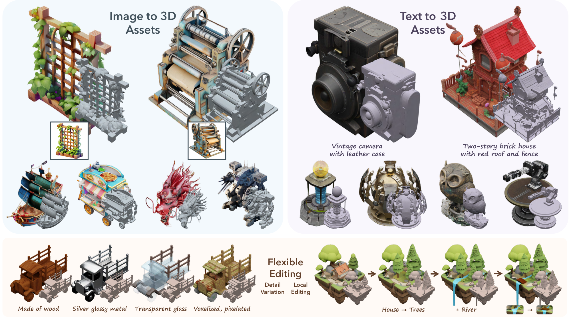
We introduce a novel 3D generation method for versatile and high-quality 3D asset creation. The cornerstone is a unified Structured LATent (SLat) representation which allows decoding to different output formats, such as Radiance Fields, 3D Gaussians, and meshes. This is achieved by integrating a sparsely-populated 3D grid with dense multiview visual features extracted from a powerful vision foundation model, comprehensively capturing both structural (geometry) and textural (appearance) information while maintaining flexibility during decoding. We employ rectified flow transformers tailored for SLat as our 3D generation models and train models with up to 2 billion parameters on a large 3D asset dataset of 500K diverse objects. Our model generates high-quality results with text or image conditions, significantly surpassing existing methods, including recent ones at similar scales. We showcase flexible output format selection and local 3D editing capabilities which were not offered by previous models.
Executive Summary: TRELLIS introduces a unified structured latent representation (SLat) that enables high-quality 3D asset generation from text or image prompts while supporting multiple output formats. The core challenge addressed is that existing 3D generative models produce lower visual quality than leading 2D systems and remain tied to single representations such as meshes, Radiance Fields, or 3D Gaussians, forcing trade-offs between geometry accuracy and appearance detail and preventing a consistent large-scale modeling approach.
The work sets out to demonstrate that a single latent space can encode both coarse geometry and fine appearance information sufficiently well to decode into any of these formats at high fidelity. The approach combines a sparsely occupied 3D grid of active voxels with dense visual features aggregated from multiview renderings through a pretrained DINOv2 vision model. Two separate rectified-flow transformer models—one operating on a compressed dense structure and one on the sparse local latents—are trained end-to-end on approximately 500,000 curated 3D assets using models up to two billion parameters.
Quantitative and qualitative results show clear gains over prior methods. On the held-out Toys4k benchmark the largest model records the highest prompt-alignment scores and the lowest distributional distances across appearance, geometry, and point-cloud metrics. User studies with more than one hundred participants indicate strong preference for TRELLIS outputs, with 67 percent of votes for text-to-3D cases and 94 percent for image-to-3D cases. Reconstruction experiments further confirm that the same latent can be decoded into Gaussians, Radiance Fields, or meshes with superior fidelity in both appearance and surface detail compared with recent latent representations. In addition, the explicit separation of structure and local features enables practical editing operations—detail variation across an entire object or region-specific addition, deletion, or replacement—without retraining or fine-tuning.
These capabilities matter because they reduce the fragmentation that currently forces separate pipelines for geometry, texturing, and downstream rendering or simulation. A single model can now serve multiple production needs while supporting rapid customization. The public release of code, models, and data lowers barriers for adoption and further research.
Next steps should focus on reducing inference cost through a single-stage generator and on separating material and lighting attributes during image-conditioned generation to support physically based rendering. Until these refinements are validated, organizations should treat the current two-stage pipeline as production-ready for preview and asset creation while budgeting additional artist polish for final lighting-critical assets. Results rest on a large but filtered training corpus and on standard reconstruction and distributional metrics; independent verification on domain-specific data remains advisable before heavy integration.
1. Introduction
Section Summary: Recent advances in AI for creating 3D objects have improved output but still lag behind 2D image generation in quality and ease of use, largely because 3D data comes in many incompatible formats such as meshes or point clouds that each handle shape or appearance differently. To address this, the authors propose a shared latent space called SLat that pairs sparse 3D structures with rich visual features from existing image models, allowing high-quality outputs that can be decoded into any common 3D representation without lengthy fitting steps. They then train large models called Trellis on this space to generate detailed 3D assets from text or images, supporting versatile uses like flexible editing while releasing all code, models, and data publicly.
While AI Generated Content (AIGC) for 3D has made tremendous progress in recent years [1, 2, 3], existing 3D generative models still fall short in generation quality compared to their 2D predecessors, where large image generation models [4, 5] have enabled ready-to-use tools that exert a profound impact on today's digital industry.
Unlike 2D images, typically represented by pixel grids, 3D data encompasses diverse representations like meshes, point clouds, Radiance Fields [6], and 3D Gaussians [7]. Each format is tailored for specific applications and may encounter difficulties when adapted for other tasks. For instance, while numerous studies [8, 9, 10, 11, 12, 13, 14] have utilized 3D representations like meshes or implicit fields [15, 16] for object geometry generation, they often falter in detailed appearance modeling compared to those relying on representations equipped with advanced volumetric rendering capabilities (e.g., 3D Gaussians and Radiance Fields). Conversely, generative models based on Radiance Fields or 3D Gaussians [17, 18, 19] excel in rendering high-quality appearances but strruggle with plausible geometry extraction. Moreover, the unique structured or unstructured characteristics of different representations complicate processing through a consistent network architecture. These issues hinder the development of a standardized 3D generative modeling paradigm, in contrast to the consensus in recent advanced 2D generation methods that learn generative models within a unified latent space [20, 4].
In this paper, we aim to develop a unified and versatile latent space that facilitates high-quality 3D generation across various representations, accommodating diverse downstream requirements. This problem is highly challenging and has rarely been addressed by previous approaches. To tackle this, our primary strategy is to introduce explicit sparse 3D structures in the latent space design. These structures enable decoding into different 3D representations by characterizing attributes within the local voxels surrounding an object, as is evidenced by recent advancements in the 3D reconstruction field [21, 22, 23]. This approach also allows for efficient high-resolution modeling by bypassing voxels without 3D information [24, 11], and introduces locality that facilitates flexible editing.
However, even with such structures, achieving high-quality decoding into different 3D representations is still non-trivial, as it requires the latent representation to encapsulate both comprehensive geometry and appearance information of the 3D assets. To address this issue, our second strategy is to equip the sparse structures with a powerful vision foundation model [25] for detailed information encoding, given its demonstrated strong 3D awareness [26] and capability for detailed representation [27]. This approach bypasses the need for a dedicated 3D encoder, and eliminates the costly pre-fitting process of aligning 3D data with specific representations [17, 19].
Given these two strategies, we introduce Structured LATents ($\textsc{SLat}$), a unified 3D latent representation for high-quality, versatile 3D generation. $\textsc{SLat}$ marries sparse structures with powerful visual representations. It defines local latents on active voxels intersecting the object's surface. The local latents are encoded by fusing and processing image features from densely rendered views of the 3D asset, while attaches them onto active voxels. These features, derived from powerful pretrained vision encoders [25], capture detailed geometric and visual characteristics, complementing the coarse structure provided by the active voxels. Different decoders can then be applied to map $\textsc{SLat}$ to diverse 3D representations of high quality.
Building on $\textsc{SLat}$, we train a family of large 3D generation models, dubbed $\textsc{Trellis}$ in this paper, with text prompts or images as conditions. A two stage pipeline is applied which first generates the sparse structure of $\textsc{SLat}$, followed by generating the latent vectors for non-empty cells. We employ rectified flow transformers as our backbone models and adapt them properly to handle the sparsity in $\textsc{SLat}$. We train $\textsc{Trellis}$ with up to 2 billion parameters on a large dataset of carefully-collected 3D assets. Through extensive experiments, we show that our model can create high-quality 3D assets with detailed geometry and vivid texture, significantly surpassing previous methods. Moreover, it can easily generate 3D assets with different output formats to meet diverse downstream requirements.
We summarize the notable features of our method below:
- High quality. It produces diverse 3D assets at high-quality with intricate shape and texture details.
- Versatile generation. It takes text or image prompts and can generate various final 3D representations including but not limited to Radiance Fields, 3D Gaussians, and meshes.
- Flexible editing. It enables flexible tuning-free 3D editing such as the deletion, addition, and replacement of local regions, guided by text or image prompts.
- Fitting-free training. No 3D fitting is needed for the training objects in the entire process.
Given these strong performance and multifold advantages, we believe our new models can serve as powerful 3D generation foundations and unlock new possibilities for the 3D vision community. We hope our work can shed some light on 3D-representation-agnostic asset modeling, in contrast to the field's relentless pursuit of and adaptation to new representations. All our code, model, and data are released to facilitate reproduction and downstream applications.
2. Related Works
Section Summary: Recent work on 3D generative models began with GAN-based approaches that struggled to scale, then shifted to diffusion models operating on point clouds, voxels, and other representations, though direct generation in raw 3D space remained inefficient. To improve quality and speed, many researchers now train models in compact latent spaces, yet these methods often compromise on fine surface details, accurate geometry, or the ability to produce complete textured assets without extra steps. An alternative line of work instead harnesses pre-trained 2D image generators to create 3D objects through distillation or multi-view rendering, but these outputs tend to suffer from geometric inconsistencies, prompting interest in newer rectified flow models as a potentially more scalable option for high-quality 3D synthesis.
3D generative models.
Early 3D generation methods primarily leveraged Generative Adversarial Nets (GANs) [28] to model 3D distributions [29, 30, 31, 32, 33, 34, 35], but faced challenges in scaling to more diverse scenarios. Later approaches employed diffusion models [36, 37] for various representations like point clouds [38, 39], voxel grids [40, 41, 42], Triplanes [43, 44, 17, 45], and 3D Gaussians [19, 46]. Some alternatives [47, 48] adopted GPT-style autoregressive models [49] for mesh generation. Despite these advancements, efficiency remains a challenge for generative modeling in raw data space.
To enhance both quality and efficiency, recent studies have resorted to generation in a more compact latent space [20]. Some methods [50, 51, 13, 14, 52, 53, 54, 11] mainly focused on shape modeling, often requiring an additional texturing phase for complete 3D asset generation. Among them, a few approaches [9, 12] incorporated appearance information, but faced difficulties to model highly detailed appearance due to their surface representations. Other works [55, 18, 56, 57] built latent representations for Radiance Fields or 3D Gaussians, which may pose challenges for accurate surface modeling. [58] encoded both geometry and appearance using latent primitives, but its pre-fitting process is both costly and lossy. In this work, we aim to build a versatile latent space that supports decoding into various 3D representations of high quality.
3D creation with 2D generative models.
Instead of directly training 3D generative models, some recent methods leveraged 2D generative models to create 3D assets due to their superior generalization abilities. A pivotal work, DreamFusion [1], optimized 3D assets by distilling from pre-trained image diffusion models [20], followed by a large group of successors [59, 60, 61, 62, 63] with more advanced distillation techniques. Another group of works [2, 64, 65, 66, 67, 68, 69, 70, 27, 71, 72] involves generating multiview images via 2D diffusions and reconstructing 3D assets from them. However, these 2D-assisted approaches often yield lower geometry quality compared to native 3D models learned from 3D data collections, due to inherent multiview inconsistency in 2D generative models.
Rectified flow models.
Rectified flow models [73, 74, 75] have recently emerged as a novel generative paradigm that challenges the dominance of diffusions [36, 37]. Recent works [4, 76] have demonstrated the effectiveness of them for large-scale image and video generation. In this paper, we also apply rectified flow models and demonstrate their abilities for 3D generation at scale.
3. Methodology
Section Summary: The methodology generates high-quality 3D assets from text or image inputs by first encoding objects into a compact structured latent called SLat. This consists of a sparse set of local feature vectors placed on the voxels of a 64^3 grid that intersect the object’s surface, capturing both coarse shape and fine appearance details. The latents are produced by aggregating DINOv2 features from many rendered views and training a sparse transformer VAE; two rectified-flow transformers then generate the grid structure and its latents, which specialized decoders can turn into 3D Gaussians, radiance fields, or meshes.
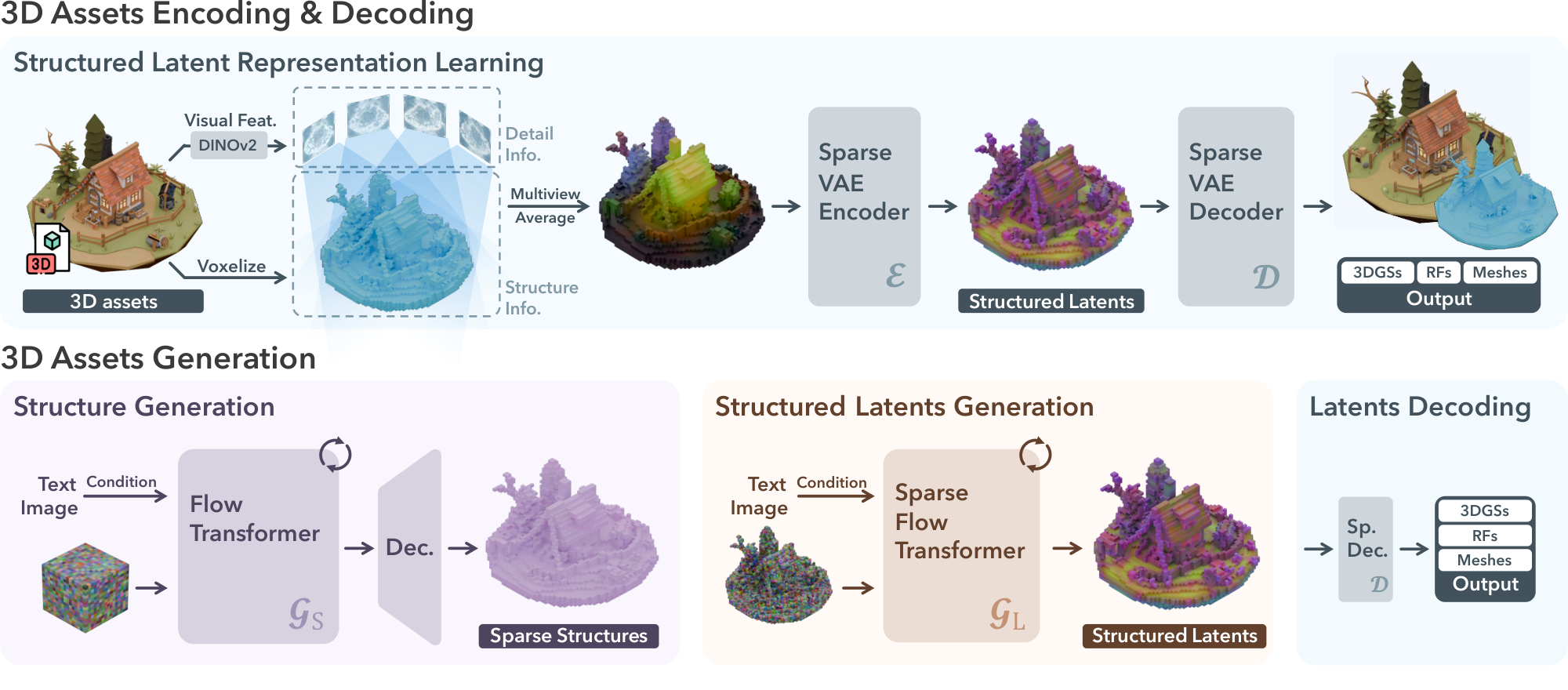
We aim to generate high-quality 3D assets in various 3D representation formats given text or image conditions. Figure 2 shows an overview, with details described below.
3.1 Structured Latent Representation
For a 3D asset $\mathcal{O}$, we encode its geometry and appearance information using a unified structured latent representation $\boldsymbol{z}$, which defines a set of local latents on a 3D grid:
$ \boldsymbol{z} = {(\boldsymbol{z}_i, \boldsymbol{p}i)}{i=1}^{L}, \quad \boldsymbol{z}_i\in\mathbb{R}^C, \ \boldsymbol{p}_i\in {0, 1, \ldots, N-1} ^3,\tag{1} $
where $\boldsymbol{p}_i$ is the positional index of an active voxel in the 3D grid intersecting with the surface of $\mathcal{O}$, $\boldsymbol{z}_i$ denotes a local latent attached to the corresponding voxel, the derivation of which will be described later, $N$ is the spatial length of the 3D grid, and $L$ is the total number of active voxels. Intuitively, the active voxels ${\boldsymbol{p}_i}$ outline the coarse structure of the 3D asset, while the latents ${\boldsymbol{z}_i}$ capture finer details of appearance and shape. Together, these structured latents encompass the entire surface of $\mathcal{O}$, effectively capturing both the overall form and intricate details.
Due to the sparsity of 3D data, the number of active voxels is significantly smaller than the total size of the grid, i.e., $L \ll N^3$, allowing to be constructed at a relatively high resolution. By default, we set $N=64$ which leads to an average value of $L=20$ K.
3.2 Structured Latents Encoding and Decoding
With the structured latent representation, we develop an effective encoding scheme to encode 3D assets to it, and introduce different decoders for reconstruction across various 3D representations. The details are outlined below.
Visual feature aggregation.
We first convert each 3D asset $\mathcal{O}$ into a voxelized feature $\boldsymbol{f}={(\boldsymbol{f}_i, \boldsymbol{p}i)}{i=1}^{L}$. Here, $\boldsymbol{p}_i$ is the active voxels as defined in Equation 1, and $\boldsymbol{f}_i$ is a visual feature recording detailed structure and appearance information of the local region.
To derive $\boldsymbol{f}_i$ for each active voxel, we aggregate features extracted from dense multiview images of $\mathcal{O}$. We render images from randomly sampled camera views on a sphere and extract feature maps using a pre-trained DINOv2 encoder [25]. Each voxel is projected onto the multiview feature maps to retrieve features at corresponding locations, and their average is used as $\boldsymbol{f}_i$, as shown in Figure 2 (left-top). We set $\boldsymbol{f}$ to match the resolution of the structured latents $\boldsymbol{z}$ (i.e., $64^3$). Empirically, this is sufficient to reconstruct the original 3D asset at high fidelity, thanks to the strong representation capabilities of DINOv2 features together with the coarse structure provided by the active voxels.
Sparse VAE for structured latents.
With the voxelized feature $\boldsymbol{f}$, we introduce a transformer-based VAE architecture for 3D assets encoding.
Specifically, an encoder $\boldsymbol{\mathcal{E}}$ first encodes $\boldsymbol{f}$ to structured latents $\boldsymbol{z}$, followed by a decoder $\boldsymbol{\mathcal{D}}$ that converts $\boldsymbol{z}$ into a 3D asset represented by certain 3D representation. Reconstruction losses are then applied between the decoded 3D assets and the ground truth to train the encoder and decoder in an end-to-end manner, along with a KL-penalty on $\boldsymbol{z_i}$ to encourage normal distribution regularization following [20].
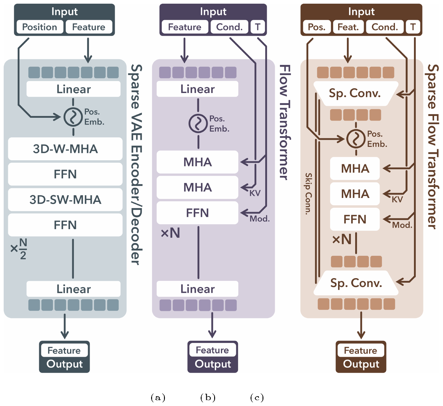
The encoder and decoder share the same transformer structure, as shown in Figure 3a. To handle sparse voxels, we serialize input features from active voxels and add sinusoidal positional encodings based on their voxel positions, creating tokens with variable context length $L$, which are subsequently processed through transformer blocks. Considering the locality characteristic of the latents, we incorporate shifted window attention [77, 78] in 3D space to enhance local information interaction, which also improves efficiency compared to a full attention implementation.
Decoding into versatile formats.
Our structured latents support decoding into diverse 3D representations, such as 3D Gaussians, Radiance Fields, and meshes, via respective decoders: $\boldsymbol{\mathcal{D}}\mathrm{GS}$, $\boldsymbol{\mathcal{D}}\mathrm{RF}$, and $\boldsymbol{\mathcal{D}}_\mathrm{M}$. These decoders share the same architecture except for their output layers, and can be trained using specific reconstruction losses tailored to their representations:
(a) 3D Gaussians. The decoding process is formulated as:
$ \boldsymbol{\mathcal{D}}_GS !:{(\boldsymbol{z}_i, \boldsymbol{p}i)}{i=1}^{L}! \rightarrow !{{(\boldsymbol{o}_i^k, \boldsymbol{c}_i^k, \boldsymbol{s}i^k, \alpha_i^k, \boldsymbol{r}i^k)}{k=1}^{K}}{i=1}^{L}, $
where each $\boldsymbol{z}_i$ is decoded into $K$ Gaussians with position offsets $\boldsymbol{o}$, colors $\boldsymbol{c}$, scales $\boldsymbol{s}$, opacities $\alpha$, and rotations $\boldsymbol{r}$. To maintain locality of $\boldsymbol{z_i}$, we constrain the final positions $\boldsymbol{x}$ of the Gaussians to the vicinity of their active voxel: $ \boldsymbol{x}^k_i = \boldsymbol{p}_i + \mathrm{tanh}(\boldsymbol{o}^k_i)$. The reconstruction losses consist of $\mathcal{L}_1$, D-SSIM and LPIPS [79] between rendered Gaussians and the ground truth images.
(b) Radiance Fields. The decoding process is defined as:
$ \boldsymbol{\mathcal{D}}_RF !:{(\boldsymbol{z}_i, \boldsymbol{p}i)}{i=1}^{L}! \rightarrow !{(\boldsymbol{v}_i^x, \boldsymbol{v}_i^y, \boldsymbol{v}_i^z, \boldsymbol{v}i^c)}{i=1}^{L}, $
where $\boldsymbol{v}_i^\mathrm{x}, \boldsymbol{v}_i^\mathrm{y}, \boldsymbol{v}_i^\mathrm{z}\in\mathbb{R}^{16\times 8}$ and $\boldsymbol{v}_i^\mathrm{c}\in\mathbb{R}^{16\times 4}$ are the CP-decomposition of a local radiance volume at $8^3$ following Strivec [23], while the reconstruction losses are similar to those for Gaussians.
(c) Meshes. The decoding process is as follows:
$ \boldsymbol{\mathcal{D}}_M !:{(\boldsymbol{z}i, \boldsymbol{p}i)}{i=1}^{L}! \rightarrow !{{(\boldsymbol{w}i^j, d_i^j)}{j=1}^{64}}{i=1}^{L}, $
where $\boldsymbol{w}_i^j\in\mathbb{R}^{45}$ are the flexible parameters in FlexiCubes [22] and $d_i^j\in\mathbb{R}^{8}$ is signed distance values for the eight vertices of the corresponding voxel. We append two convolutional upsampling blocks after the transformer backbone to increase the final output resolution to $256^3$ (i.e., each $\boldsymbol{z_i}$ for a grid of $4^3$), extract meshes from 0-level isosurfaces, and compute $\mathcal{L}_1$ between rendered depth (normal) maps and their ground truth as the reconstruction losses.
In practice, we adopt Gaussians to learn the encoder and decoder end-to-end due to their high fidelity and efficiency. For other output formats, we simply freeze the learned encoder and train their decoders from scratches as described above. Despite trained with Gaussians, the learned structured latents can faithfully reconstruct other formats, demonstrating strong extensibility (See Table 1). We leave more implementation details in Appendix A.2.
3.3 Structured Latents Generation
We introduce a two-stage generation pipeline to generate the structured latents, which first generates the sparse structure, followed by the local latents attached to it. For modeling the latent distribution, we employ rectified flow models [75]. We will first provide a brief introduction to these models before detailing our generation pipeline.
Rectified flow models.
Rectified flow models use a linear interpolation forward process, $\boldsymbol{x}(t)=(1-t)\boldsymbol{x}_0+t\boldsymbol{\epsilon}$, which interpolates between data samples $\boldsymbol{x}0$ and noises $\boldsymbol{\epsilon}$ with a timestep $t$. The backward process is represented as a time-dependent vector field, $\boldsymbol{v}(\boldsymbol{x}, t) = \nabla_t\boldsymbol{x}$, moving noisy samples toward the data distribution, and can be approximated with a neural network $\boldsymbol{v}\theta$ by minimizing the conditional flow matching (CFM) objective [75]:
$ \mathcal{L}{CFM}(\theta)=\mathbb{E}{t, \boldsymbol{x}0, \boldsymbol{\epsilon}} | \boldsymbol{v}\theta(\boldsymbol{x}, t)-(\boldsymbol{\epsilon}-\boldsymbol{x}_0) |^ 2_2.\tag{2} $
Sparse structure generation.
In the first stage, we aim to generate the sparse structure ${\boldsymbol{p}i}{i=1}^{L}$. To enable this with a tensorized neural network, we convert the sparse active voxels into a dense binary 3D grid $\boldsymbol{O} \in {0, 1}^{N\times N\times N}$, setting voxel values to $1$ if active, and $0$ otherwise.
Directly generating the dense grid $\boldsymbol{O}$ is computationally expensive. We introduce a simple VAE with 3D convolutional blocks to compress it into a low-resolution feature grid $\boldsymbol{S}\in\mathbb{R}^{D\times D\times D \times C_\mathrm{S}}$. Since $\boldsymbol{O}$ represents only coarse geometry, this compression is nearly lossless, enhancing efficiency significantly. It also converts the discrete values in $\boldsymbol{O}$ into continuous features suited for rectified flow training.
We introduce a simple transformer backbone $\boldsymbol{\mathcal{G}}_{\mathrm{S}}$ for generating $\boldsymbol{S}$, as shown in Figure 3b. An input dense noisy grid is serialized, combined with positional encodings (as in Section 3.2), and fed into the transformer for denoising. Timestep information is incorporated using adaptive layer normalization (adaLN) and a gating mechanism [80]. Conditions are injected through cross attention layers as keys and values. For text conditions, we use features from a pretrained CLIP [81] model. For image conditions, we adopt visual features from DINOv2. The denoised feature grid $\boldsymbol{S}$ is decoded into the discrete grid $\boldsymbol{O}$, and further converted back to active voxels ${\boldsymbol{p}i}{i=1}^{L}$ as the final sparse structure.
Structured latents generation.
In the second stage, we generate latents ${\boldsymbol{z}i}{i=1}^{L}$ given the structure ${\boldsymbol{p}i}{i=1}^{L}$ using a transformer $\boldsymbol{\mathcal{G}}_{\mathrm{L}}$ designed for sparse structures (Figure 3c).
Instead of directly serializing input noisy latents as in the sparse VAE encoder in Section 3.2, we improve efficiency by packing them into a shorter sequence before serialization, similarly as done by DiT [80]. Due to our sparse structure, we apply a downsampling block with sparse convolutions [82] to pack latents within a $2^3$ local region, followed by multiple time-modulated transformer blocks. A convolutional upsampling block is appended at the end of the transformer, with skip connections to the downsampling block that facilitates spatial information flow. Like in $\boldsymbol{\mathcal{G}}_{\mathrm{S}}$, timesteps are integrated via adaLN layers, and text/image conditions are injected through cross-attentions.
We train $\boldsymbol{\mathcal{G}}{\mathrm{S}}$ and $\boldsymbol{\mathcal{G}}{\mathrm{L}}$ separately using the CFM objective in Equation 2. After training, structured latents $\boldsymbol{z}={(\boldsymbol{z}i, \boldsymbol{p}i)}{i=1}^{L}$ can be sequentially generated by the two models and converted into high-quality 3D assets in various formats by different decoders: $\boldsymbol{\mathcal{D}}{\mathrm{GS}}$, $\boldsymbol{\mathcal{D}}{\mathrm{RF}}$, and $\boldsymbol{\mathcal{D}}{\mathrm{M}}$. See Appendix A for more details.
3.4 3D Editing with Structured Latents
Our method supports flexible 3D editing and we present two simple tuning-free editing strategies.
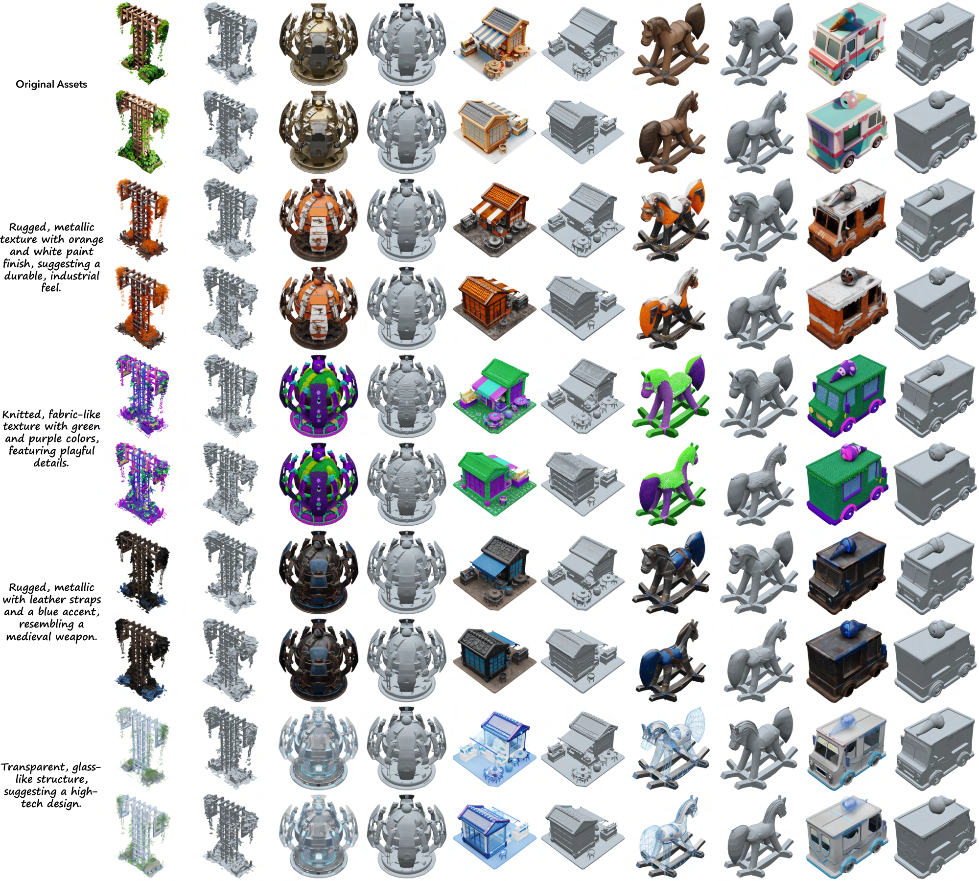
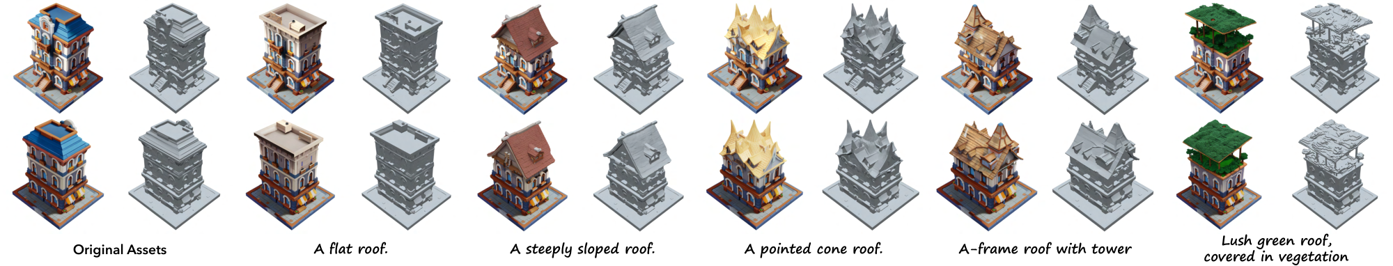
Detail variation.
The separation between the structure and latents enables detail variation of 3D assets without affecting the overall coarse geometry. This can be easily accomplished by preserving the asset's structure and executing the second generation stage with different text prompts.
Region-specific editing.
The locality of $\textsc{SLat}$ allows for region-specific editing by altering voxels and latents in targeted areas while leaving others unchanged. To this end, we adapt Repaint [83] to our two-stage generation pipeline. Given a bounding box for the voxels to be edited, we modify our flow models' sampling processes to create new content in that region, conditioned on the unchanged areas and any provided text or image prompts. Consequently, the first stage generates new structures within the specified region, and the second stage produces coherent details.
4. Experiments
Section Summary: In the experiments section, the authors describe training their models on roughly 500,000 high-quality 3D objects collected from public datasets, using rendered images and AI-generated captions to learn the mapping from text or image prompts to detailed 3D outputs. They compare their approach against prior methods by measuring how accurately it reconstructs shapes and appearances, as well as how well it generates new 3D assets, and report superior performance on standard metrics like visual fidelity and geometric accuracy. Visual examples and user studies further illustrate that the resulting 3D models exhibit richer details, more consistent structures, and higher overall quality than those produced by existing techniques.
Implementation details.
For training, we carefully collect approximately 500K high-quality 3D assets from 4 public datasets: Objaverse (XL) [84], ABO [85], 3D-FUTURE [86], and HSSD [87]. We render 150 images per asset, and employ GPT-4o [88] for captioning. Data augmentation is applied to both text and image prompts: texts are summarized to varying lengths, and images are rendered with different FoVs. We use classifier-free guidance (CFG) [89] with a drop rate of $0.1$ and AdamW [90] optimizer with a learning rate of $1e-4$. We train three models with total parameters of 342M (Basic), 1.1B (Large), and 2B (X-Large). The XL model is trained with 64 A100 GPUs (40G) for 400K steps with a batchsize of 256. At inference, CFG strength is set to $3$ and sampling steps to $50$.
For quantitative evaluations, we use Toys4k [91], which is not part of our training set or those of the compared methods. For visual results, comparisons, and user studies, we use text generated by GPT-4 [92] and images by DALL-E 3 [93]. Our method uses decoded Gaussians for appearance evaluation and meshes for geometry, unless specified otherwise. Refer to the suppl. material for more details.
\begin{tabular}{c|cc|cccc}
  \toprule
  \multirow{2}{*}{\textbf{Method}} & \multicolumn{2}{c|}{\textbf{Appearance}} & \multicolumn{4}{c}{\textbf{Geometry}} \\
     & \textbf{PSNR $\uparrow$} & \textbf{LPIPS $\downarrow$} & \textbf{CD $\downarrow$} & \textbf{F-score $\uparrow$} & \textbf{PSNR-N $\uparrow$} & \textbf{LPIPS-N $\downarrow$} \\
     \midrule
  LN3Diff & 26.44 & 0.076 & 0.0299 & 0.9649 & 27.10 & 0.094 \\
  3DTopia-XL &
  25.34$^{\dag}$ & 0.074$^{\dag}$ & 0.0128 & 0.9939 & 31.87 & 0.080 \\
  CLAY & -- & -- & 0.0124 & 0.9976 & 35.35 & 0.035 \\
        \textbf{Ours} & \textbf{32.74}/\tiny{32.19$^{\ddagger}$} & \textbf{0.025}/\tiny{0.029$^{\ddagger}$} & \textbf{0.0083} & \textbf{0.9999} & \textbf{36.11} & \textbf{0.024} \\
        \bottomrule
    \end{tabular}
\begin{tabular}{c|cccccc|cccccc}
        \toprule
        \multirow{2}{*}{\textbf{Method}} & \multicolumn{6}{c|}{\textbf{Text-to-3D}} & \multicolumn{6}{c}{\textbf{Image-to-3D}} \\
  & $\textbf{CLIP}\!\uparrow$ & $\textbf{FD}_\textbf{incep}\!\downarrow$ & $\textbf{KD}_\textbf{incep}\!\downarrow$ & $\textbf{FD}_\textbf{dinov2}\!\downarrow$ & $\textbf{KD}_\textbf{dinov2}\!\downarrow$ & $\textbf{FD}_\textbf{point}\!\downarrow$ & $\textbf{CLIP}\!\uparrow$ & $\textbf{FD}_\textbf{incep}\!\downarrow$ & $\textbf{KD}_\textbf{incep}\!\downarrow$ & $\textbf{FD}_\textbf{dinov2}\!\downarrow$ & $\textbf{KD}_\textbf{dinov2}\!\downarrow$ & $\textbf{FD}_\textbf{point}\!\downarrow$ \\
        \midrule
        Shap-E & 25.04 & 37.93 & 0.78 & 497.17 & 49.96 & 6.58 & 82.11 & 34.72 & 0.87 & 465.74 & 62.72 & 8.20 \\
        LGM & 24.83 & 36.18 & 0.77 & 507.47 & 61.89 & 24.73 & 83.97 & 26.31 & 0.48 & 322.71 & 38.27 & 15.90 \\
  InstantMesh & 25.56 & 36.73 & 0.62 & 478.92 & 49.77 & 10.79 & 84.43 & 20.22 & 0.30 & 264.36 & 25.99 & 9.63 \\
        3DTopia-XL & 22.48$^{\dag}$ & 53.46$^{\dag}$
 & 1.39$^{\dag}$ & 756.37$^{\dag}$ & 87.40$^{\dag}$ & 13.72 & 78.45$^{\dag}$ & 37.68$^{\dag}$ & 1.20$^{\dag}$ & 437.37$^{\dag}$ & 53.24$^{\dag}$ &	18.21 \\
  Ln3Diff & 18.69 & 71.79 & 2.85 & 976.40 & 154.18 & 19.40 & 82.74 & 26.61 & 0.68 & 357.93 & 50.72 & 7.86 \\
  GaussianCube & 24.91 & 27.35 & 0.30 & 460.07 & 39.01 & 29.95 & -- & -- & -- & -- & -- & -- \\
        \textbf{Ours L} & $\underline{26.60}$ & $\underline{20.54}$ & \textbf{0.08} & $\underline{238.60}$ & $\underline{4.24}$ & $\underline{5.24}$ & \textbf{85.77} & \textbf{9.35} & \textbf{0.02} & \textbf{67.21} & \textbf{0.72} & \textbf{2.03} \\
        \textbf{Ours XL} & \textbf{26.70} & \textbf{20.48} & \textbf{0.08} & \textbf{237.48} & \textbf{4.10} & \textbf{5.21} & -- & -- & -- & -- & -- & -- \\
        \bottomrule
    \end{tabular}
4.1 Reconstruction Results
We first assess the reconstruction fidelity of different latent representations. We compare $\textsc{SLat}$ with alternatives also learned from large-scale data: latent point clouds from 3DTopia-XL [58], latent vector sets from CLAY [14], and latent triplanes from LN3Diff [18].
For appearance fidelity, we report PSNR and LPIPS between rendered reconstruction results and ground truth. For geometry quality, we use Chamfer Distance (CD) and F-score to assess overall shape accuracy, and PSNR and LPIPS for rendered normal maps to evaluate surface details.
As shown in Table 1, our method outperforms all baselines across all evaluated metrics. For geometry, it even surpasses CLAY which focuses solely on shape encoding. The high-fidelity reconstruction results under diverse output formats demonstrates strong versatility of $\textsc{SLat}$.
4.2 Generation Results
In this section, we evaluate our generation quality. We first present various 3D generation results of our method, and then compare with other baseline methods.
Text/image-to-3D generation.
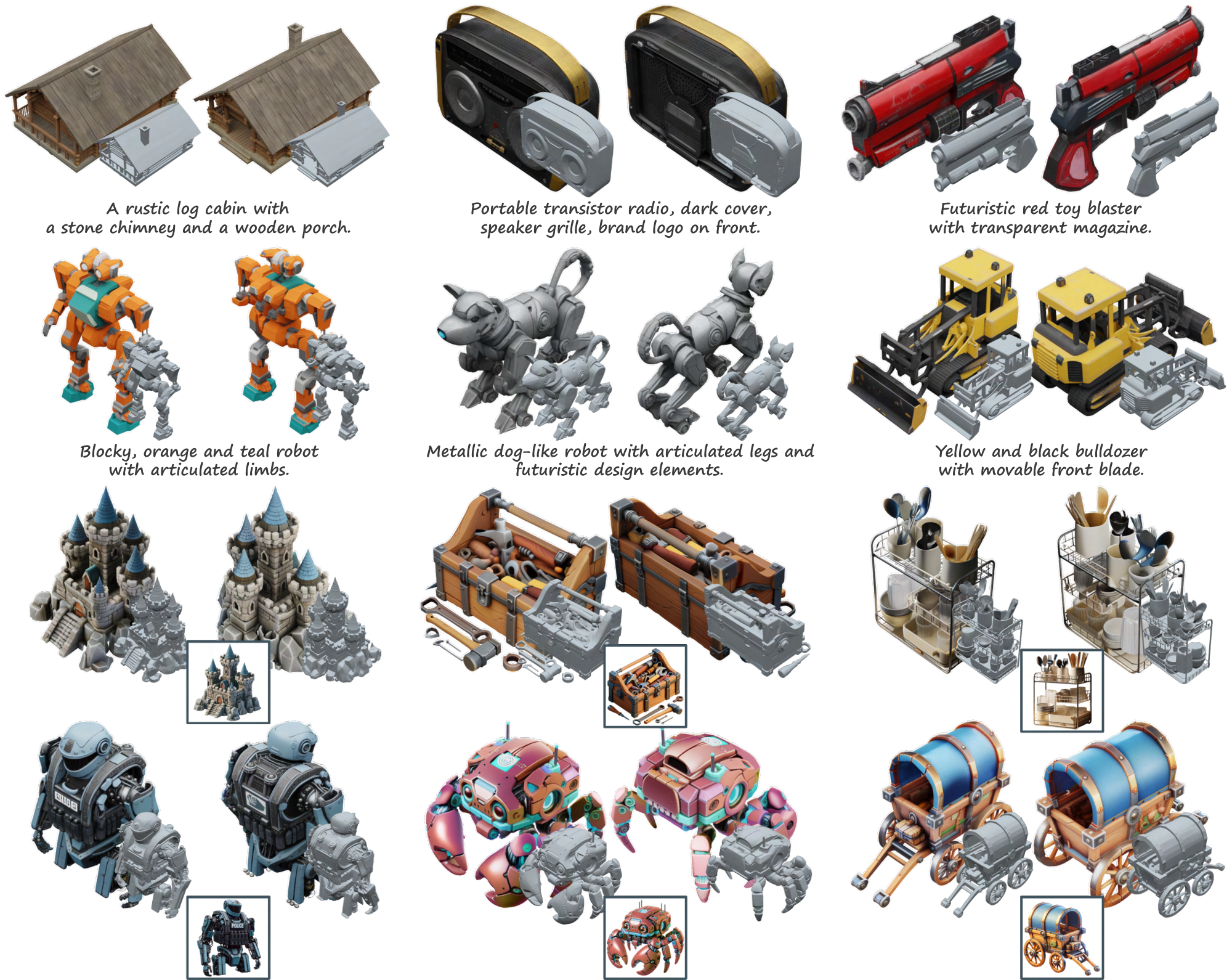
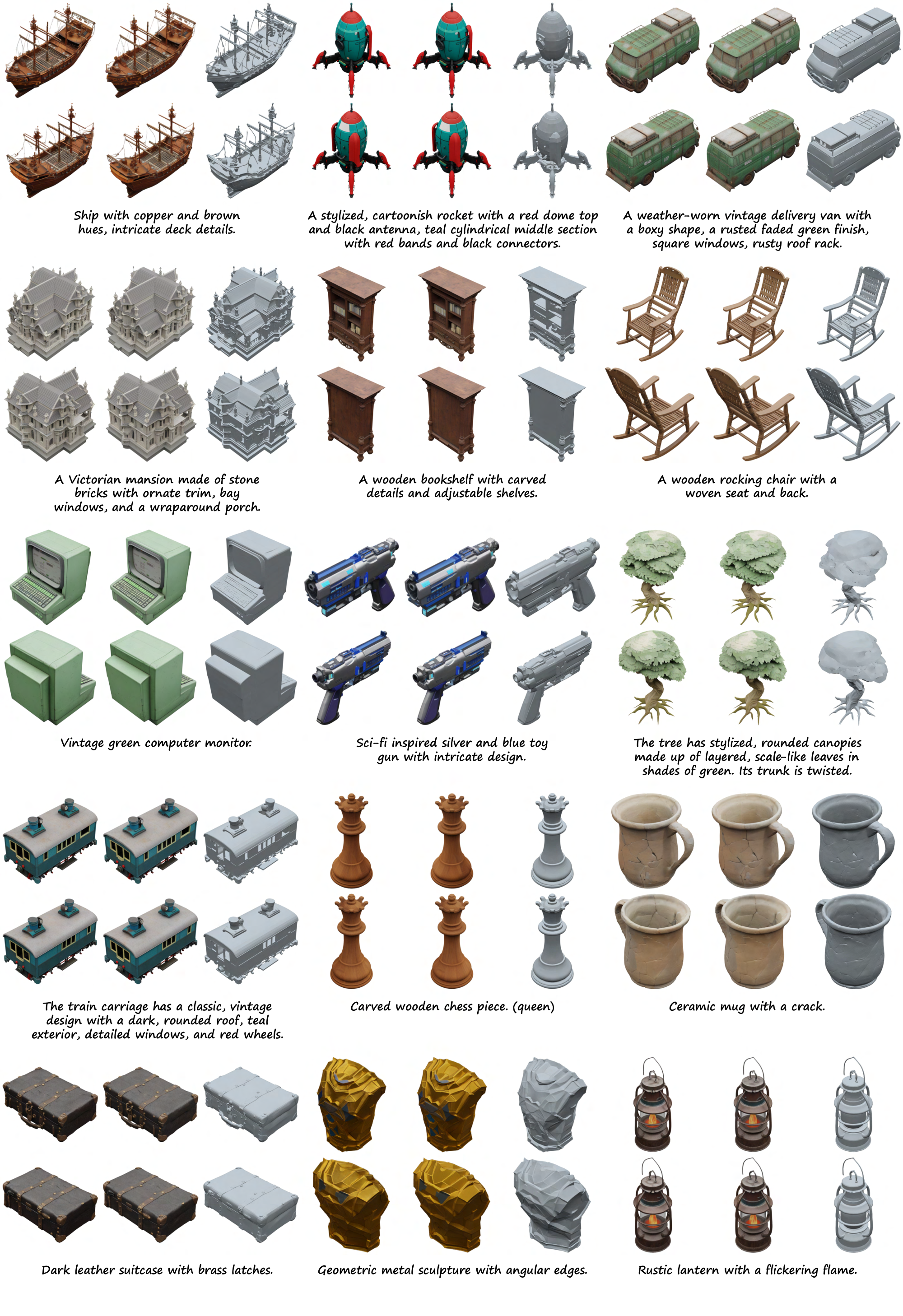
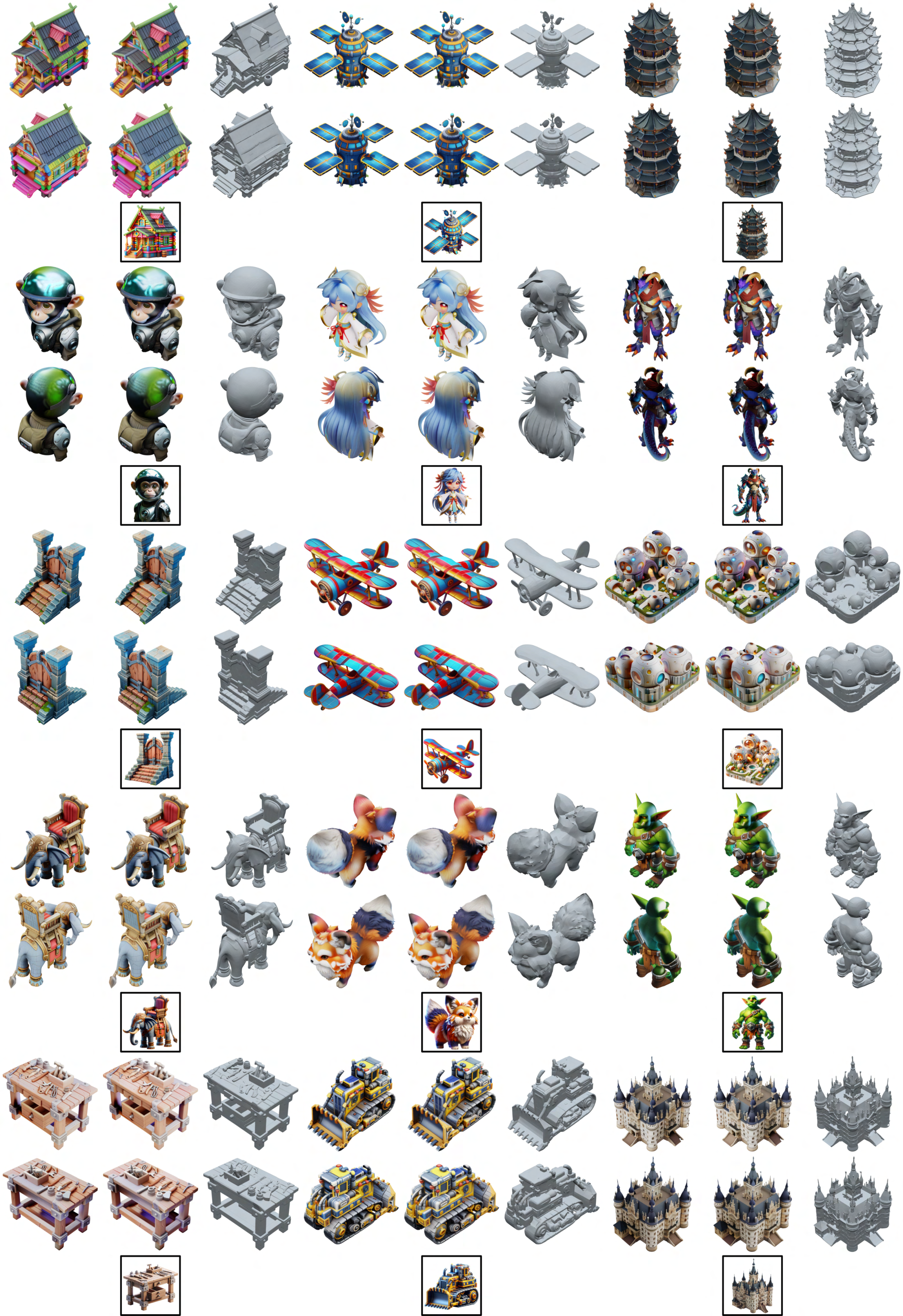
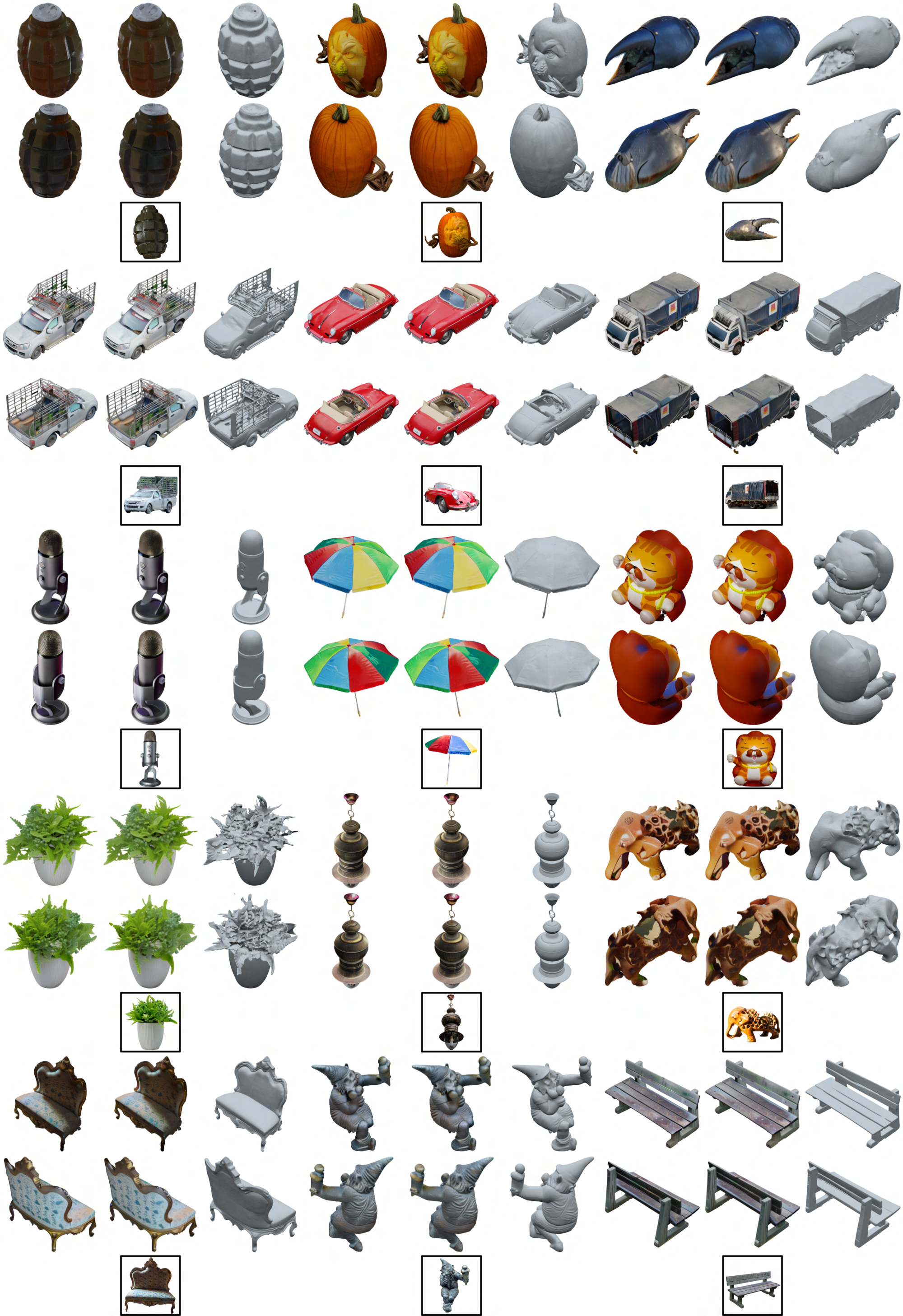
Figure 4 showcases 3D assets generated by our method, where the text and image prompts are given below. We present two views for each asset: front-left and back-right.
Upon visual inspection, our method produces 3D assets with an unprecedented level of quality. The generated appearances possess vibrant colors and vivid details, such as the radio speaker's grille and the toy blaster's scratches. The geometries reveal complex structures and fine shape details, with superior surface properties like flat faces and sharp edges (e.g., the bulldozer's hollow driving cab and the equipment on the police robot). It can even handle translucent objects such as the drinking glasses on the kitchen rack. Additionally, the generated contents closely match the elements from the provided text (e.g., the log cabin with a stone chimney and wooden porch) and faithfully adhere to details from input images (e.g., the castle with brick walls). More results can be found in Figure 1 and Appendix D.
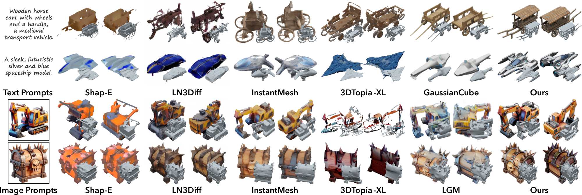
Qualitative comparisons.
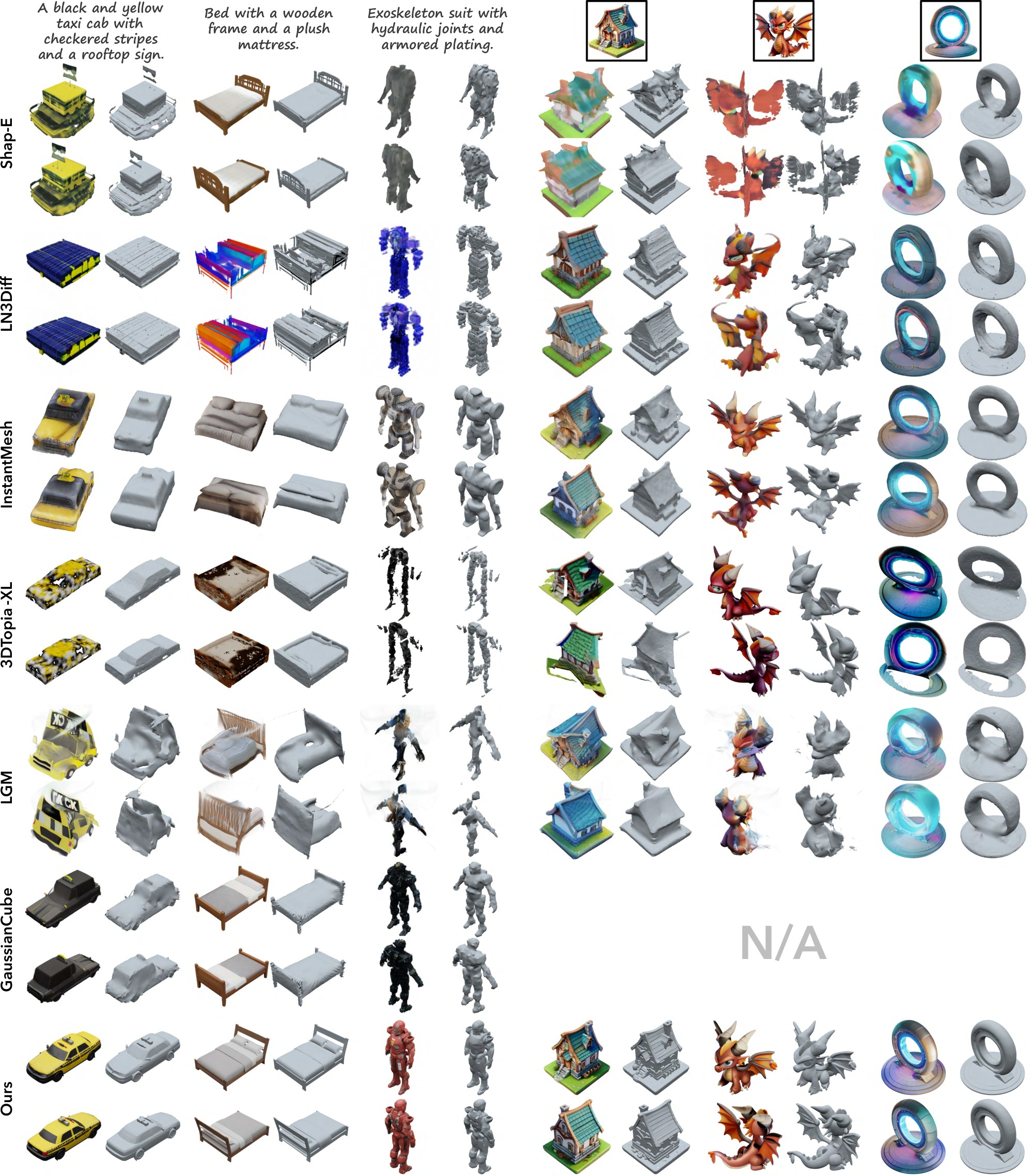
We compare our approach with existing 3D generation methods that utilize different generative paradigms, latent representations, and output formats, including 2D-assisted methods: InstantMesh [94] and LGM [69]; and 3D generative approaches: GaussianCube [19], Shap-E [55], 3DTopia-XL, and LN3Diff. We do not compare with CLAY in this phase, as their generation models are currently unavailable to us.
We begin by presenting visual comparisons in Figure 5. Our method outperforms all previous approaches, offering not only more vivid appearances and finer geometries but also more precise alignment with the provided text and image prompts. It excels at producing intricate and coherent details, whereas alternatives experience varying degrees of quality degradation: The 2D-assisted methods suffer from structural distortion due to multiview inconsistencies inherent in the 2D generative models they rely on; other 3D generative approaches encounter featureless appearances and geometries, constrained by the limited reconstruction fidelity of their latent representations. GaussianCube and LGM do not provide plausible geometries, which is an inherent issue with their 3D Gaussian representations.
Quantitative comparisons.
Furthermore, we perform quantitative comparisons using text and image prompts in Toys4k and present the results in Table 2. We utlize Fréchet distance (FD) [95] and kernel distance (KD) [96] with various feature extractors (i.e., Inception-v3 [97], DINOv2, and PointNet++ [98]) to assess overall quality of the generated outputs, and use CLIP score [81] to evaluate the consistency between the generated results and the input prompts. As demonstrated, our method significantly surpasses previous methods across all evaluated metrics.
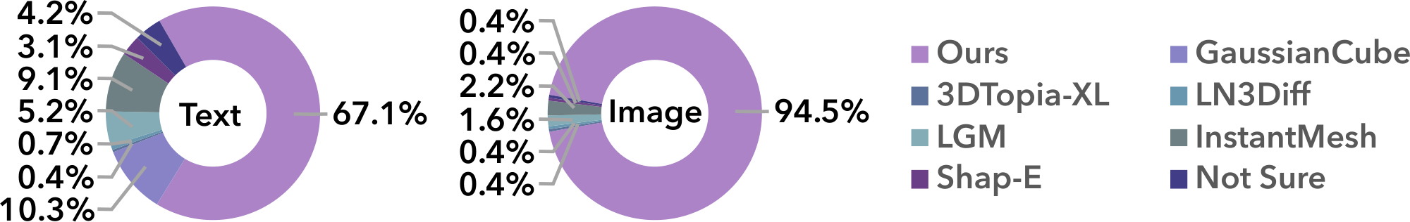
User study.
In addition, we conduct a user study with over 100 participants to compare different methods based on human preferences. We leverage 68 AI-generated text prompts and 67 image prompts, and create 3D assets from them via each method without any curation. As illustrated in Figure 6, our method is strongly preferred by users due to its significant improvements in generation quality. Details of the user study can be found in Appendix C.2.
: Table 3: Ablation study on the size of $\textsc{SLat}$.
| Resolution | Channel | PSNR $\uparrow$ | LPIPS $\downarrow$ |
|---|---|---|---|
| 32 | 16 | 31.64 | 0.0297 |
| 32 | 32 | 31.80 | 0.0289 |
| 32 | 64 | $\underline{31.85}$ | $\underline{0.0283}$ |
| 64 | 8 | 32.74 | 0.0250 |
\begin{tabular}{cc|cc|cc}
        \toprule
        & \multirow{2}{*}{\textbf{Method}} & \multicolumn{2}{c|}{\textbf{Training set}} & \multicolumn{2}{c}{\textbf{Toys4k}}\\
  && $\textbf{CLIP}\!\uparrow$ & $\textbf{FD}_\textbf{dinov2}\!\downarrow$ & $\textbf{CLIP}\!\uparrow$ & $\textbf{FD}_\textbf{dinov2}\!\downarrow$ \\
        \midrule
  \multirow{2}{*}{Stage 1}
  & Diffusion & 25.09 & 132.71 & 25.86 & 295.90 \\
  & Rectified flow & \textbf{25.40} & \textbf{113.42} & \textbf{26.37} & \textbf{269.56} \\
        \midrule
  \multirow{2}{*}{Stage 2}
  & Diffusion & 25.58 & 100.88 & 26.45 & 244.08 \\
  & Rectified flow & \textbf{25.65} & \textbf{95.97} & \textbf{26.61} & \textbf{240.20} \\
        \bottomrule
    \end{tabular}
\begin{tabular}{c|cc|cc}
  \toprule
  \multirow{2}{*}{\textbf{Method}} & \multicolumn{2}{c|}{\textbf{Training set}} & \multicolumn{2}{c}{\textbf{Toys4k}}\\
  & $\textbf{CLIP}\!\uparrow$ & $\textbf{FD}_\textbf{dinov2}\!\downarrow$ & $\textbf{CLIP}\!\uparrow$ & $\textbf{FD}_\textbf{dinov2}\!\downarrow$ \\
  \midrule
  B & 25.41 & 121.45 & 26.47 & 265.26 \\
  L & $\underline{25.62}$ & $\underline{99.92}$ & $\underline{26.60}$ & $\underline{238.60}$ \\
  XL & \textbf{25.71} & \textbf{93.96} & \textbf{26.70} & \textbf{237.48} \\
  \bottomrule
  \end{tabular}
4.3 Ablation Study
We conduct ablation studies to validate the design choices of our method under the text-to-3D configuration.
Size of structured latents.
To determine the size for $\textsc{SLat}$, we train sparse VAEs with varying latent resolutions and channels. As shown in Table 3, while the performance under $32^3$ is quite good, it tends to plateau as the number of latent channels increases. Switching to $64^3$ provides a significant boost. We prioritize quality over efficiency and adopt $64^3$ as our default setting for $\textsc{SLat}$.
Rectified flow v.s. diffusion.
We compare rectified flow models with a widely used diffusion baseline [80] in Table 4. We independently alter the generation method at each stage using the large model size, while maintaining the XL model unchanged for the other stages. As shown, replacing diffusion models with rectified flow models at any stage improves both generation quality and prompt alignment.
Model size.
We examine the model's performance with varying numbers of parameters. Table 5 shows that increasing the model size consistently improves the generation performance on both training distribution and Toys4k.
4.4 Applications
We demonstrate tuning-free applications of our method by utilizing the editing strategies described in Section 3.4.
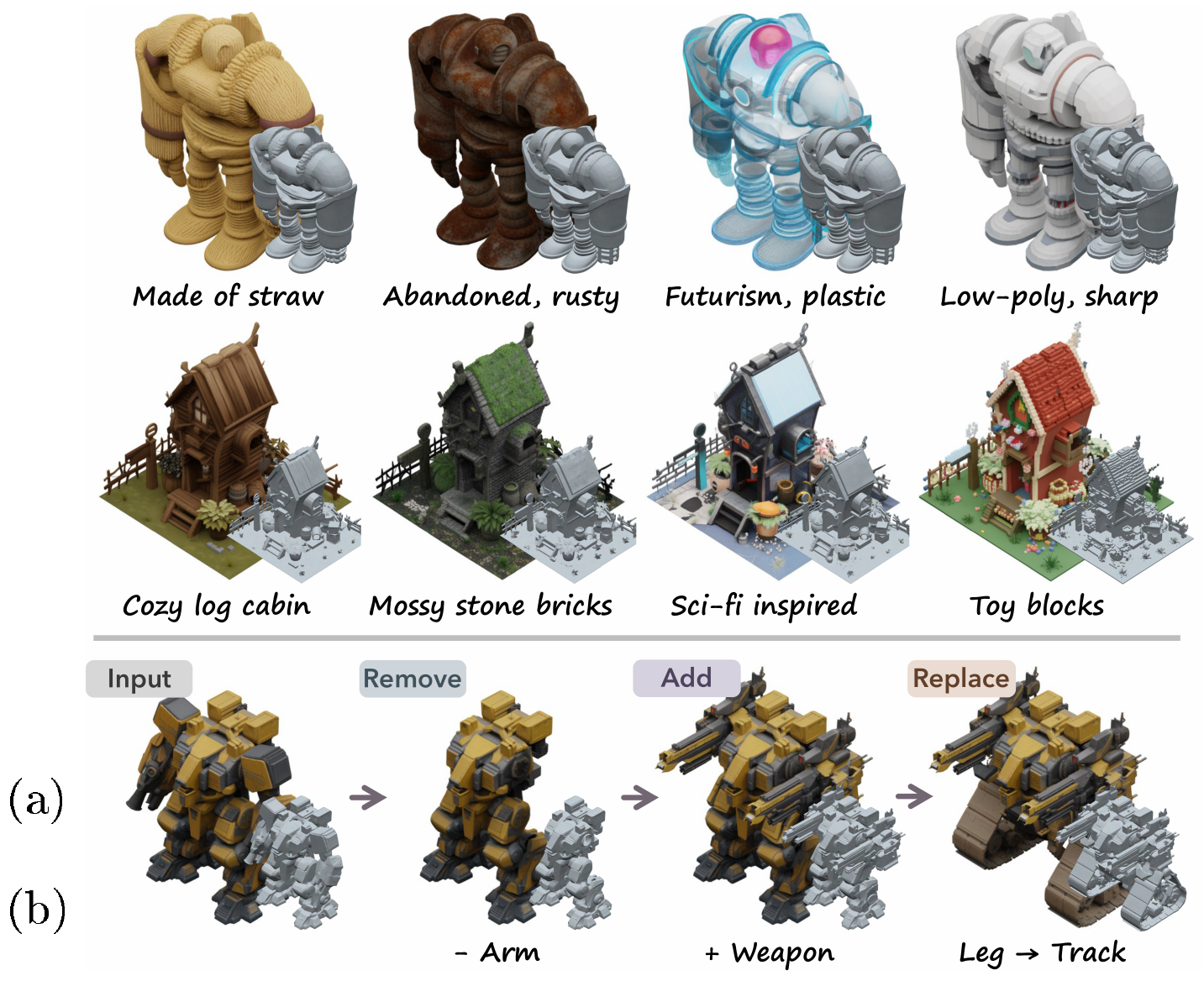
3D asset variations.
Figure 1 and Figure 7a show 3D asset variation results. Our method produces variants adhering to the overall shape of the given structures while exhibiting diverse appearance and geometry details guided by the text.
Region-specific editing of 3D assets.
Figure 1 and Figure 7b illustrate the editing sequences of two 3D assets, involving removal, addition, and replacement operations. Corresponding prompts (either text or image) for each step are provided. Our method enables detailed local region editing, such as adding a river and bridge in the island example.
5. Conclusion
Section Summary: The researchers developed a new method for creating high-quality, flexible 3D models that can be easily edited and adapted for different uses. Their approach captures both shape and surface details from multiple 2D images and processes them through large-scale AI models in two main steps to generate the final assets. Experiments confirmed that the results outperform earlier techniques across quality and versatility, pointing to broad applications in digital design and production.
We introduced a novel 3D generation method for versatile and high-quality 3D asset creation. At its core lies $\textsc{SLat}$, a structured latent representation that allows decoding to versatile output formats by comprehensively encoding both geometry and appearance information into localized latents anchored on a sparse 3D grid, where the latents are fused and processed from dense multiview image features extracted by a powerful vision foundation model. We proposed a two-stage generation pipeline utilizing rectified flow transformers tailored for $\textsc{SLat}$ generation at scale. Extensive experiments demonstrated the superiority of our method in 3D generation, in terms of quality, versatility, and editability, highlighting its strong potential for a wide range of real-world applications in digital production.
Appendix
Section Summary: The appendix presents detailed network configurations and architectural specifications for the various encoders, decoders, and generators employed in the paper, including their layer counts, dimensions, parameter sizes, and specialized components such as 3D convolutional U-Nets, shifted-window attention, and sparse convolutions. It explains how these elements, like query-key normalization and custom downsamplers, address practical issues in processing sparse 3D voxel data and maintaining training stability. Additional notes cover training procedures, hyperparameters, and loss designs for components such as the sparse structure VAE.
: Table 6: Network configurations used in this paper. SW stands for Shifted Window", MSA and MCA for Multihead Self-Attention" and Multihead Cross-Attention", and Sp. Conv. for Sparse Convolution".
| Network | #Layer | #Dim. | #Head | Block Arch. | Special Modules | #Param. |
|---|---|---|---|---|---|---|
| $\boldsymbol{\mathcal{E}}_\mathrm{S}$ | – | – | – | – | 3D Conv. U-Net | 59.3M |
| $\boldsymbol{\mathcal{D}}_\mathrm{S}$ | – | – | – | – | 3D Conv. U-Net | 73.7M |
| $\boldsymbol{\mathcal{E}}$ | 12 | 768 | 12 | 3D-SW-MSA + FFN | 3D Swin Attn. | 85.8M |
| $\boldsymbol{\mathcal{D}}_\mathrm{GS}$ | 12 | 768 | 12 | 3D-SW-MSA + FFN | 3D Swin Attn. | 85.4M |
| $\boldsymbol{\mathcal{D}}_\mathrm{RF}$ | 12 | 768 | 12 | 3D-SW-MSA + FFN | 3D Swin Attn. | 85.4M |
| $\boldsymbol{\mathcal{D}}_\mathrm{M}$ | 12 | 768 | 12 | 3D-SW-MSA + FFN | 3D Swin Attn. + Sp. Conv. Upsampler | 90.9M |
| $\boldsymbol{\mathcal{G}}_\mathrm{S}$-B (text ver.) | 12 | 768 | 12 | MSA + MCA + FFN | QK Norm. | 157M |
| $\boldsymbol{\mathcal{G}}_\mathrm{S}$-L (text ver.) | 24 | 1024 | 16 | MSA + MCA + FFN | QK Norm. | 543M |
| $\boldsymbol{\mathcal{G}}_\mathrm{S}$-XL (text ver.) | 28 | 1280 | 16 | MSA + MCA + FFN | QK Norm. | 975M |
| $\boldsymbol{\mathcal{G}}_\mathrm{S}$-L (image ver.) | 24 | 1024 | 16 | MSA + MCA + FFN | QK Norm. | 556M |
| $\boldsymbol{\mathcal{G}}_\mathrm{L}$-B (text ver.) | 12 | 768 | 12 | MSA + MCA + FFN | QK Norm. + Sp. Conv. Downsampler / Upsampler + Skip Conn. | 185M |
| $\boldsymbol{\mathcal{G}}_\mathrm{L}$-L (text ver.) | 24 | 1024 | 16 | MSA + MCA + FFN | QK Norm. + Sp. Conv. Downsampler / Upsampler + Skip Conn. | 588M |
| $\boldsymbol{\mathcal{G}}_\mathrm{L}$-XL (text ver.) | 28 | 1280 | 16 | MSA + MCA + FFN | QK Norm. + Sp. Conv. Downsampler / Upsampler + Skip Conn. | 1073M |
| $\boldsymbol{\mathcal{G}}_\mathrm{L}$-L (image ver.) | 24 | 1024 | 16 | MSA + MCA + FFN | QK Norm. + Sp. Conv. Downsampler / Upsampler + Skip Conn. | 600M |
A. More Implementation Details
A.1 Network Architectures
The networks used in our method primarily consist of transformers [99], augmented by a few specialized modules. The configurations and statistics for each network are listed in Table 6. In particular, $\boldsymbol{\mathcal{E}}\mathrm{S}$ and $\boldsymbol{\mathcal{D}}\mathrm{S}$ compose the VAE designed for sparse structures, as discussed in Section 3.3 in the main paper. The remaining networks are also defined in the main paper. Below, we provide detailed descriptions of the architectures of the specialized modules introduced.
3D convolutional U-net.
The VAE for sparse structures ($\boldsymbol{\mathcal{E}}\mathrm{S}$ and $\boldsymbol{\mathcal{D}}\mathrm{S}$) is introduced to enhance the efficiency of the structure generator $\boldsymbol{\mathcal{G}}\mathrm{S}$ and to convert the binary grids of active voxels into continuous latents for flow training. Its architecture is similar to the VAEs in LDM [20], but it employs 3D convolutions and omits self-attention metchanisms. $\boldsymbol{\mathcal{E}}\mathrm{S}$ ($\boldsymbol{\mathcal{D}}_\mathrm{S}$) consists of a series of residual blocks and downsampling (upsampling) blocks, reducing the spatial size from $64^3$ to $16^3$. The feature channels are set to $32$, $128$, $512$ for spatial sizes of $64^3$, $32^3$, $16^3$, respectively. The latent channel dimension is set to $8$. We utilize pixel shuffle [100] in the upsampling block and replace group normalizations with layer normalizations.
3D shifted window attention.
In the VAE for structured latents ($\textsc{SLat}$), we employ 3D shifted window attention to facilitate local information interaction and improve efficiency. Specifically, we partition the $64^3$ space into $8^3$ windows, with tokens inside each window performing self-attention independently. Despite the potential variation in the number of tokens per window, this challenge can be efficiently addressed using modern attention implementations (e.g., FlashAttention [101] and xformers [102]). The transformer blocks alternate between non-shifted window attention and window attention shifted by $(4, 4, 4)$, ensuring that the windows in adjacent layers overlap uniformly.
QK normalization.
Similar to the challenges reported in SD3 [4], we encounter training instability caused by the exploding norms of queries and keys within the multi-head attention blocks. To mitigate this issue, we follow [4] to apply root mean square normalizations [103] (RMSNorm) to the queries and keys before sending them into the attention operators.
Sparse convolutional downsampler/upsampler.
In $\boldsymbol{\mathcal{D}}\mathrm{M}$ and $\boldsymbol{\mathcal{G}}\mathrm{L}$, it is necessary to alter the spatial size of sparse tensors to increase the resolution of the SDF grid for meshes and to improve the efficiency of the $\textsc{SLat}$ generator, respectively. To achieve this, we employ downsampling and upsampling blocks equipped with sparse convolutions [82]. These blocks are composed of residual networks with two sparse convolutional layers, skip connections with optional linear mappings, and pooling or unpooling operators. We use average pooling and nearest-neighbor unpooling. For $\boldsymbol{\mathcal{G}}\mathrm{L}$, given that the structures of $64^3$ are pre-determined, we only average the features from active voxels within each $2^3$ pooling window and recover the $64^3$ structures during unpooling. This is done by assigning values to active voxels from their nearest neighbors in the $32^3$ space. For $\boldsymbol{\mathcal{D}}\mathrm{M}$, we simply subdivide each voxel into $2^3$, resulting in a new sparse tensor with doubled spatial dimensions in each upsampling block.
A.2 Training Details
We provide more details about the training process for each model, including hyperparameter tuning, algorithm details, and loss function designs.
Sparse structure VAE.
We frame the training of the sparse structure VAE as a binary classification problem, given the binary nature of the active voxels. Each decoded voxel is classified as either positive (active) or negative (inactive). Due to the imbalance between positive and negative labels, where active voxels are sparser than inactive ones, we adopt the Dice loss [104] to effectively manage this disparity.
Structured latent VAE.
For the versatile decoding of $\textsc{SLat}$, we implement decoders for various 3D representations, namely $\boldsymbol{\mathcal{D}}\mathrm{GS}$ for 3D Gaussians [7], $\boldsymbol{\mathcal{D}}\mathrm{RF}$ for Radiance Fields [6], and $\boldsymbol{\mathcal{D}}_\mathrm{M}$ for meshes. We provide detailed information on their respective training processes.
(a) 3D Gaussians. Following Mip-Splatting [105], we address aliasing by setting the minimal scale for Gaussians to $9e-4$ and the variance of the screen space Gaussian filter to $0.1$. The value $9e-4$ is derived from the assumption of a $512^3$ sampling rate within the $(-0.5, 0.5)^3$ cube. For each active voxel, 32 Gaussians are predicted (i.e., $K=32$ in the main paper). Since original density control schemes are not applicable when Gaussians are predicted by neural networks, we employ regularizations for volume [106] and opacity of the Gaussians to prevent their degeneration, specifically to avoid them becoming excessively large or transparent. The full training objective is:
$ \mathcal{L}{GS}=\mathcal{L}{recon}+\mathcal{L}{vol}+\mathcal{L}{\alpha}, $
where $\mathcal{L}{\mathrm{recon}}$, $\mathcal{L}{\mathrm{vol}}$ and $\mathcal{L}_{\alpha}$ are defined below:
$ \begin{split}\mathcal{L}{recon}=\mathcal{L}1&+0.2(1-SSIM)+0.2{LPIPS}, \\mathcal{L}{vol}&=\frac1{LK}\sum{i=1}^{L}\sum_{k=1}^K\prod\boldsymbol{s}i^k, \\mathcal{L}{\alpha}&=\frac1{LK}\sum_{i=1}^{L}\sum_{k=1}^K(1-\alpha_i^k)^2.\end{split}\tag{3} $
(b) Radiance Fields. We predict 4 orthogonal vectors $\boldsymbol{v}_i^\mathrm{x}, \boldsymbol{v}_i^\mathrm{y}, \boldsymbol{v}_i^\mathrm{z}, \boldsymbol{v}_i^\mathrm{c}$ for each active voxel. These vectors represent the CP-decomposition [107] of a local $8^3$ radiance volume $\boldsymbol{V}\in\mathbb{R}^{8\times 8\times 8\times 4}$:
$ \boldsymbol{V}{i, xyzc}=\sum{r=1}^{R}\boldsymbol{v}{i, rx}^x\boldsymbol{v}{i, ry}^y\boldsymbol{v}{i, rz}^z\boldsymbol{v}{i, rc}^c. $
The last dimension of $\boldsymbol{V}$, which has a size of 4, contains the color and density information. We set the rank $R=16$. The recovered local volumes are then assembled according to the position of their respective active voxels, forming a $512^3$ radiance field. Additionally, we implement an efficient differentiable renderer using CUDA, which enables real-time rendering by integrating sorting, ray marching, radiance integration, and the CP reconstruction into a single kernel. The training objective of $\boldsymbol{\mathcal{D}}\mathrm{RF}$ is $\mathcal{L}{\mathrm{recon}}$ as defined in Equation 3.
(c) Meshes. We increase the spatial size of sparse structures from $64^3$ to $256^3$, by appending two aforementioned sparse convolutional upsamplers after the transformer backbone. For $\boldsymbol{\mathcal{D}}_\mathrm{M}$, although our primary focus is on shape (geometry), we also predict colors and normal maps for the meshes. As a result, the final output for each high-resolution active voxel is:
$ (\boldsymbol{w}_i^j, \boldsymbol{d}_i^j, \boldsymbol{c}_i^j, \boldsymbol{n}_i^j). $
Here, $\boldsymbol{w}_i^j = (\boldsymbol{\alpha}_i^j, \boldsymbol{\beta}_i^j, \gamma_i^j, \boldsymbol{\delta}_i^j)$ are the flexible parameters defined in FlexiCubes [22], where $\boldsymbol{\alpha}_i^j \in\mathbb{R}^{8}$ and $\boldsymbol{\beta}_i^j \in\mathbb{R}^{12}$ are interpolation weights per voxel, $\gamma_i^j \in\mathbb{R}$ is the splitting weights per voxel, and $\boldsymbol{\delta}_i^j \in\mathbb{R}^{8\times 3}$ is per vertex deformation vectors of the voxel. In addition, $\boldsymbol{d}_i^j \in\mathbb{R}^{8}$ is the signed distance values for the eight vertices of the voxel, $\boldsymbol{c}_i^j \in\mathbb{R}^{8\times 3}$ denotes vertex colors, and $\boldsymbol{n}_i^j \in\mathbb{R}^{8\times 3}$ represents vertex normals. Since each vertex is connected to multiple voxels, we derive the final vertex attributes (i.e., $\boldsymbol{\delta}$, $\boldsymbol{d}$, $\boldsymbol{c}$, and $\boldsymbol{n}$) by averaging the predictions from all associated voxels.
To simplify implementation, we attach the sparse structure to a dense grid for differentiable surface extraction using FlexiCubes. For all inactive voxels in the dense grid, we set their signed distance values to $1.0$ and all other associated attributes to zero. We then extract meshes from the 0-level iso-surfaces of the dense grid. For each mesh vertex, its associated attributes (i.e., $\boldsymbol{c}$ and $\boldsymbol{n}$) are interpolated from those of the corresponding grid vertices. We utilize Nvdiffrast [108] to render the extracted mesh along with its attributes, producing a foreground mask $\boldsymbol{M}$, a depth map $\boldsymbol{D}$, a normal map $\boldsymbol{N}_m$ directly derived from the mesh, an RGB image $\boldsymbol{C}$, and a normal map $\boldsymbol{N}$ from the predicted normals. The training objective is then defined as follows:
$ \mathcal{L}_{M}=\mathcal{L}_geo+0.1\mathcal{L}color+\mathcal{L}{reg}, $
where $\mathcal{L}\mathrm{geo}$ and $\mathcal{L}\mathrm{color}$ are written as:
$ \begin{split} \mathcal{L}geo = \mathcal{L}1(\boldsymbol{M})+&10 \mathcal{L}{Huber}(\boldsymbol{D})+\mathcal{L}{recon}(\boldsymbol{N}{m}), \ \mathcal{L}color = &\mathcal{L}{recon}(\boldsymbol{C}) + \mathcal{L}{recon}(\boldsymbol{N}). \end{split} $
Here, $\mathcal{L}{\mathrm{recon}}$ is defined identically to 3. Finally, $\mathcal{L}{\mathrm{reg}}$ consists of three terms:
$ \mathcal{L}reg = \mathcal{L}{consist} +\mathcal{L}{dev} + 0.01\mathcal{L}{tsdf}, $
where $\mathcal{L}{\mathrm{consist}}$ penalizes the variance of attributes associated with the same voxel vertex, $\mathcal{L}{\mathrm{dev}}$ is a regularization term defined in FlexiCubes to ensure plausible mesh extraction, and $\mathcal{L}_{\mathrm{tsdf}}$ enforces the predicted signed distance values $\boldsymbol{d}$ to closely match the distances between grid vertices and the extracted mesh surface, helping to stablize the training process in its early stages.
Rectified flow models.
We employ rectified flow models $\boldsymbol{\mathcal{G}}\mathrm{S}$ and $\boldsymbol{\mathcal{G}}\mathrm{L}$ for sparse structure generation and structured latent generation, respectively. During training, we alter the timestep sampling distribution, replacing the $\mathrm{logitNorm}(0, 1)$ distribution used in SD3 with $\mathrm{logitNorm}(1, 1)$. We evaluate their performance at each stage of our generation pipeline using the Toys4k dataset. As shown in Table 7, the latter provides a better fit for our task and we set it as the default setting.
\begin{tabular}{cc|cc}
        \toprule
        & \textbf{Distribution} & $\textbf{CLIP}\!\uparrow$ & $\textbf{FD}_\textbf{dinov2}\!\downarrow$ \\
        \midrule
  \multirow{2}{*}{Stage 1}
  & $\mathrm{logitNorm}(0, 1)$ & 26.03 & 287.33 \\
  & $\mathrm{logitNorm}(1, 1)$ & \textbf{26.37} & \textbf{269.56} \\
        \midrule
  \multirow{2}{*}{Stage 2}
  & $\mathrm{logitNorm}(0, 1)$ & \textbf{26.61} & 242.36 \\
  & $\mathrm{logitNorm}(1, 1)$ & \textbf{26.61} & \textbf{240.20} \\
        \bottomrule
    \end{tabular}
B. Data Preparation Details
Recognizing the critical importance of both the quantity and quality of training data for scaling up the generative models, we carefully curate our training data from currently available open-source 3D datasets to construct a high-quality, large-scale 3D dataset. Moreover, we employed state-of-the-art multimodal model, GPT4o [88], to caption each 3D asset, ensuring precise and detailed text descriptions. This facilitates accurate and controllable generation of 3D assets from text prompts. In the following sections, we will first briefly introduce each 3D dataset utilized, and then provide details about our data curation pipeline. In addition, we provide a comprehensive explanation of both the captioning process and our rendering settings.
B.1 3D Datasets
Objaverse-XL [84].
Objaverse-XL is the largest open-source 3D dataset, comprising over 10 million 3D objects sourced from diverse platforms such as GitHub, Thingiverse, Sketchfab, Polycam, and the Smithsonian Institution. This extensive collection includes manually designed objects, photogrammetry scans of landmarks and everyday items, as well as professional scans of historic and antique artifacts. Despite its large scale, Objaverse-XL is quite noisy, containing a significant number of low-quality objects, such as those with missing parts, low-resolution textures, and simplified geometries. Therefore, we include only the objects from Sketchfab (also known as ObjaverseV1 [109]) and GitHub in our training dataset and perform a thorough filtering process to clean the dataset.
ABO [85].
ABO includes about 8K high-quality 3D models provided by Amazon.com. These models are designed by artists and feature complex geometries and high-resolution materials. The dataset encompasses 63 categories, primarily focusing on furniture and interior decoration.
3D-FUTURE [86].
3D-FUTURE contains around 16.5K 3D models created by experienced designers for industrial production, offering rich geometric details and informative textures. This dataset specifically focuses on 3D furniture shapes designed for household scenarios.
HSSD [87].
HSSD is a high-quality, human-authored synthetic 3D scene dataset designed to test navigation agent generalization to realistic 3D environments. It includes a total of 14K 3D models, primarily assets of indoor scenes such as furniture and decorations.
Toys4k [91].
Toys4k contains approximately 4K high-quality 3D objects from 105 object categories, featuring a diverse set of object instances within each category. Since previous works have not utilized this dataset for training, we leverage it as our testing dataset to evaluate the generalization of our model.
B.2 Data Curation Pipeline
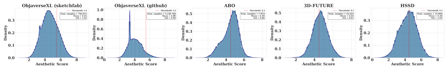
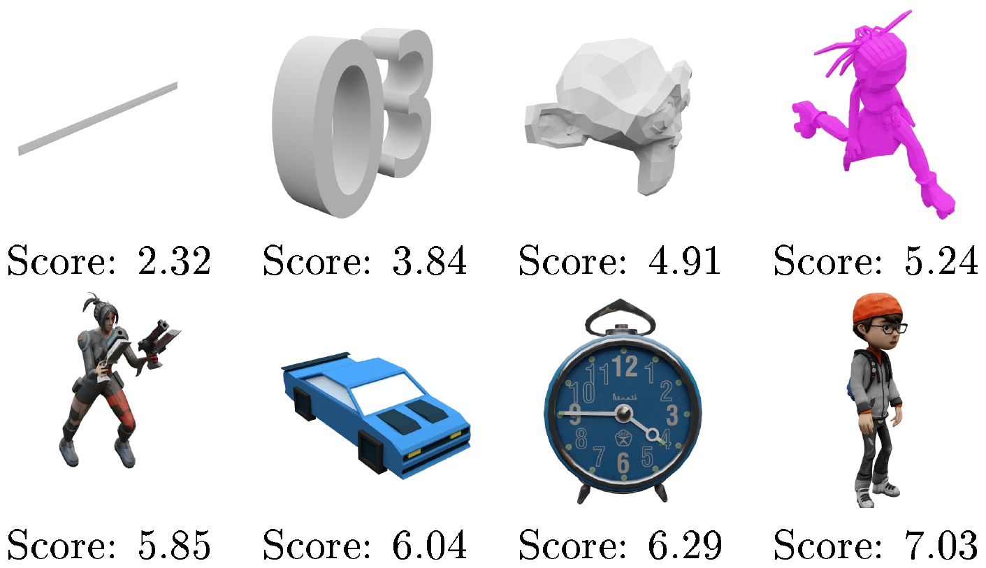
To ensure high-quality training data, we implement a systematic curation process. First, we render 4 images from uniformly distributed viewpoints around each 3D object. We then employ a pretrained aesthetic assessment model ^1 to evaluate the quality of each 3D asset. More specifically, we assess the average aesthetic score across 4 rendered view for each 3D object. We empirically find this scoring mechanism can effectively identify objects with poor visual quality -- those that receive low aesthetic scores typically exhibit undesirable characteristics such as minimal texturing or overly simplistic geometry. We visualize the distribution of aesthetic scores in each dataset in Figure 8, and further provide some examples in Figure 9 to illustrate the correspondance between the quality of 3D assets and their aesthetic scores. By filtering out objects with average aesthetic score below a certain aesthetic score threshold (i.e., 5.5 for Objaverse-XL and 4.5 for the other datasets), we maintain a high standard of geometric and textural complexity in our dataset. After filtering, there are about 500K high-quality 3D objects left (more details listed in Table 8), which comprise our training dataset.
\begin{tabular}{c|cc}
  \toprule
  \textbf{Source} & \textbf{Aesthetic Score Threshold} & \textbf{Filtered Size} \\
  \midrule
  ObjaverseXL (sketchfab) & 5.5 & 168307 \\
  ObjaverseXL (github) & 5.5 & 311843 \\
  ABO & 4.5 & 4485 \\
  3D-FUTURE & 4.5 & 9472 \\
  HSSD & 4.5 & 6670 \\
  \textbf{All (training set)} & -- & 500777 \\
  \midrule
  Toys4k (evaluation set) & 4.5 & 3229 \\
  \bottomrule
  \end{tabular}
B.3 Captioning Process
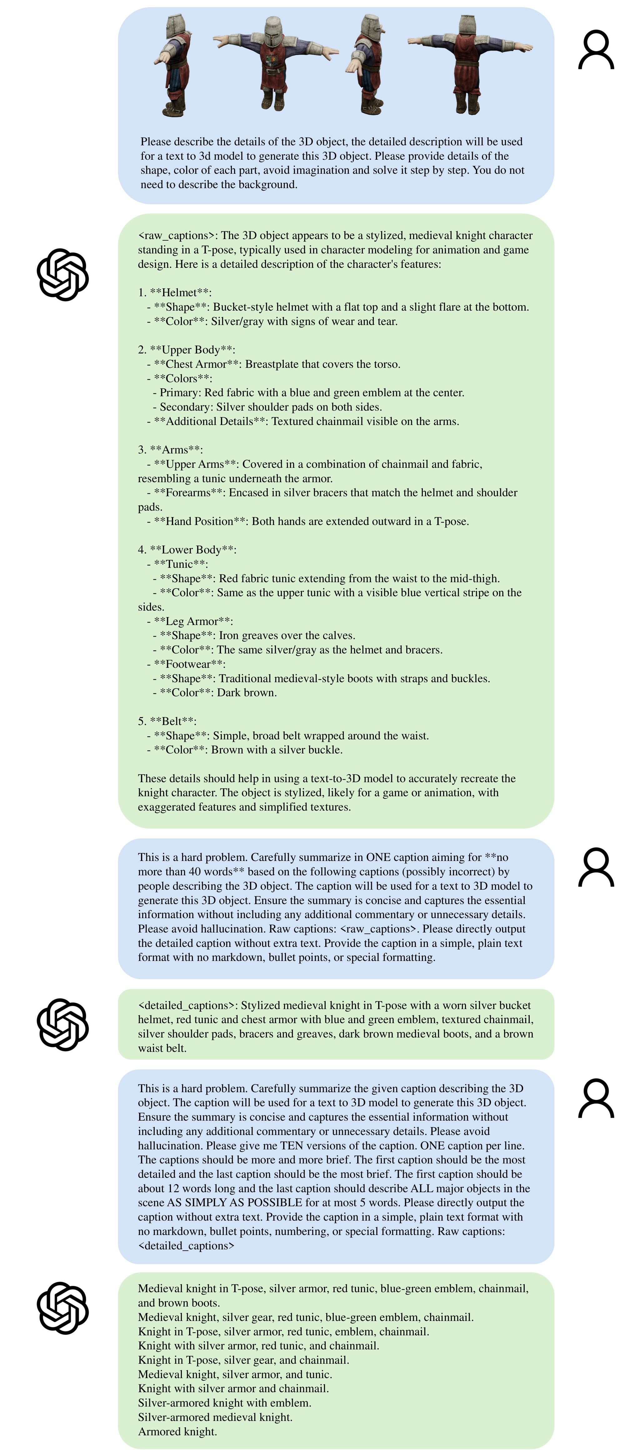
Current available captions [110] for 3D objects either suffer from poor alignment with the objects they describe or lack detailed descriptions [111], which hinders high-quality text-to-3D generation. Therefore, we carefully design a captioning process following [111] to make the model generate precise and detailed text descriptions for each 3D object. To be more specific, we first employ GPT4o to produce a highly detailed description lt;$ raw_captions gt;$ '' of the input rendered images. Subsequently, GPT4o distills the crucial information from
lt;$ detailed_captions gt;$ '', typically comprising no more than 40 words. Additionally, we summarize the lt;$ detailed_captions gt;$ '' into varying-length text prompts for augmentation in training. An illustration of the entire captioning process can be found in Figure 10, which also includes the prompts designed for GPT4o.
B.4 Rendering Process
For VAE training, we sample 150 cameras looking at the origin with a FoV of $40^\circ$, uniformly distributed across a sphere with a radius of 2. We render the assets using Blender, with a smooth area lighting. For the image-conditioned generation model, we render a different set of images with augmented FoVs ranging from $10^\circ$ to $70^\circ$, which serves as image prompts during training.
C. More Experiment Details
C.1 Evaluation Protocol
In Section 4.2 and Section 4.3 in the main paper, we conduct quantitative comparisons and ablation studies using a series of numerical metrics. We provide detailed protocols for their calculation below.
Reconstruction experiments.
We randomly sample a subset of 500 instances from the filtered Toys4k dataset, which comprises 3, 229 3D assets (see Table 8), as the evaluation set to assess the reconstruction fidelity of different latent representations. The evaluation is conducted in the following two aspects.
(a) Appearance fidelity. For each instance, we randomly sample one camera positioned on a sphere with a radius of 2, looking towards the origin with a FoV of $40^\circ$. We calculate PSNR and LPIPS between the rendered images from the reconstructed 3D assets and the ground truth images, and average the results as the final metrics. For 3DTopia-XL [58], which focuses on PBR materials, we report the reconstruction fidelity of albedo maps.
(b) Geometry accuracy. We employ Chamfer Distance (CD) and F-score of sampled point clouds to assess the overall geometry accuracy, as well as PSNR and LPIPS for rendered normal maps (i.e., PSNR-N and LPIPS-N) to evaluate surface details. Definitions for the point cloud metrics are listed below:
- Chamfer Distance:
$ \begin{split} CD(\boldsymbol{X}, \boldsymbol{Y})&=\frac1{|\boldsymbol{X}|}\sum_{\boldsymbol{x}\in\boldsymbol{X}}\min_{\boldsymbol{y}\in\boldsymbol{Y}}|\boldsymbol{x}-\boldsymbol{y}|2\&+\frac1{|\boldsymbol{Y}|}\sum{\boldsymbol{y}\in\boldsymbol{Y}}\min_{\boldsymbol{x}\in\boldsymbol{X}}|\boldsymbol{y}-\boldsymbol{x}|_2. \end{split} $
- F-score:
$ \begin{split}FN = \sum [\min_{\boldsymbol{y}\in \boldsymbol{Y}} &| \boldsymbol{x} -\boldsymbol{y}|2 > r], \FP = \sum [\min{\boldsymbol{x}\in \boldsymbol{X}} &|\boldsymbol{y} - \boldsymbol{x}|_2 > r], \TP = &|\boldsymbol{Y}| - FP, \precision = &\frac{TP}{TP+FP}, \recall = &\frac{TP}{TP+FN}, \\mathbf{F-score}(\boldsymbol{X}, \boldsymbol{Y})=&\frac{2\cdot precision\cdot recall}{precision+recall}.\end{split} $
The point clouds used to assess the overall geometry accuracy (CD and F-score with $r=0.05$) are sampled from the outer surface of the reconstructed meshes. Specifically, we render depth maps for each mesh from 100 uniformly sampled views, with camera settings identical to that for appearance evaluation. The depth maps are then unprojected to 3D points. We randomly sample 100K points from all the 3D points as the point clouds for evaluation.
For PSNR-N and LPIPS-N, as in the appearance metrics, we calculate the mean values across 500 image pairs (rendered results v.s. ground truth), with one pair per instance.
Generation experiments.
For comparisons and ablation studies regarding generation quality, we utilize two evaluation sets: a subset of Toys4k with 1, 250 randomly sampled instances and a subset of the training set with 5, 000 instances. We employ Fréchet Distance (FD) [95] and Kernel Distance (KD) [96] with various feature extractors (i.e., Inception-v3 [97], DINOv2, and PointNet++ [98]) to assess the overall quality of the generated outputs. Additionally, the CLIP score [81] is used to evaluate the consistency between the generated results and the input prompts. For each prompt in the evaluation set, we generate one asset using the generation model and use these assets as the generated set for metrics calculation. We provide detailed calculations for each metric below.
(a) Appearance quality. We employ $\mathrm{FD}\mathrm{incep}$, $\mathrm{KD}\mathrm{incep}$, $\mathrm{FD}\mathrm{dinov2}$, and $\mathrm{KD}\mathrm{dinov2}$ as evaluation metrics. For each instance, we render 4 views using cameras with yaw angles of ${0^\circ, 90^\circ, 180^\circ, 270^\circ}$, and a pitch angle of $30^\circ$. All other camera settings are consistent with those in the reconstruction experiments. The rendered images are then used to calculate different metrics. For Toys4k, we use 5, 000 images each for both the real and rendered sets, while for the training set, we use 20, 000 images.
(b) Geometry quality. We utilize $\mathrm{FD}_\mathrm{point}$. Following Point-E [38], we prepare the point clouds by sampling 4, 000 points from unprojected multiview depth maps using the farthest point sampling technique.
(c) Prompt alignment. We render 8 images per asset with yaw angles at every $45^\circ$, a pitch angle of $30^\circ$, and a radius of $2$. We calculate the cosine similarity between the CLIP features of images from the generated assets and their corresponding text or image prompts. The average of all similarities ($\times100$) is reported as the final CLIP score.
\begin{tabular}{c|cc|cc}
        \toprule
        \multirow{2}{*}{\textbf{Method}} & \multicolumn{2}{c|}{\textbf{Text-to-3D}} & \multicolumn{2}{c}{\textbf{Image-to-3D}} \\
  & $\textbf{Selections}\!\uparrow$ & $\textbf{Perentage}\!\uparrow$ & $\textbf{Selections}\!\uparrow$ & $\textbf{Perentage}\!\uparrow$ \\
        \midrule
  Not Sure & 56 & 4.2\% & 6 & 0.4\% \\
        Shap-E & 42 & 3.1\% & 6 & 0.4\% \\
        LGM & 70 & 5.2\% & 22 & 1.6\% \\
  InstantMesh & 123 & 9.1\% & 30 & 2.2\% \\
        3DTopia-XL & 5 & 0.4\% & 5 & 0.4\% \\
  Ln3Diff & 9 & 0.7\% & 6 & 0.4\% \\
        GaussianCube & 139 & 10.3\% & -- & -- \\
        \textbf{Ours} & \textbf{905} & \textbf{67.1\%} & \textbf{1277} & \textbf{94.5\%} \\
  \midrule
  \textbf{Total} & 1349 & 100\% & 1352 & 100\% \\
        \bottomrule
    \end{tabular}
C.2 User Study
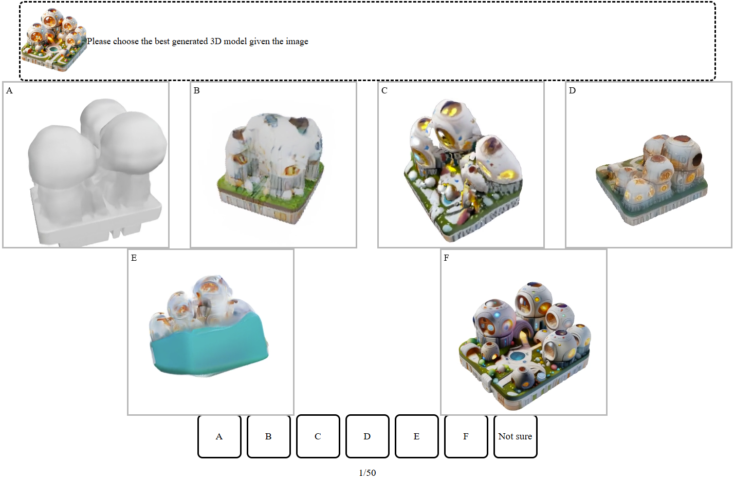
We conducted a user study to evaluate the performance of various methods based on human preferences. Participants were presented with side-by-side comparisons of 3D assets generated by different methods. In each trial, they were given a text prompt or reference image, along with several rotating videos of candidate 3D assets generated using different techniques. The interface, as depicted in Figure 11, displayed the reference image at the top, followed by options representing the generated 3D models. Participants were asked to select the model that best matched the reference image in terms of visual fidelity and overall quality, or they could choose "Not sure" if they were unable to make a decision. Each participant was assigned 50 trials, and their selections were recorded for analysis.
To ensure a diverse and unbiased evaluation, we implemented the following measures:
- The candidate 3D assets were not curated. Specifically, we sampled once per text or image prompt and used those samples directly in the study.
- The 50 trials for each participant were randomly selected from a pool of 68 text-to-3D cases and 67 image-to-3D cases. The order of candidates in each trial was also randomized.
We collected responses from 104 participants. In total, 2, 701 trials were answered, with an average of 25.97 responses each. Detailed statistics are in Figure 6.
D. More Results
D.1 3D Asset Generation
We present additional examples of 3D assets generated by our method. These include more text-to-3D results with AI-generated prompts in Figure 12 and more image-to-3D results from both AI-generated images (Figure 13) and real world images (Figure 14). For real-world images, we use segmented objects from SA-1B [112], which feature challenging materials, geometries, and camera views. Each $2\times3$ grid shows one generated asset, with front-left and back-right views in the top and bottom rows. Rendered images with 3D Gaussians (GS), Radiance Fields (RF), and meshes are displayed from left to right.
D.2 More Comparisons
In Figure 15, we provide additional comparisons of 3D assets generated by our method and those produced by alternative approaches described in Section 4.2 in the main paper.
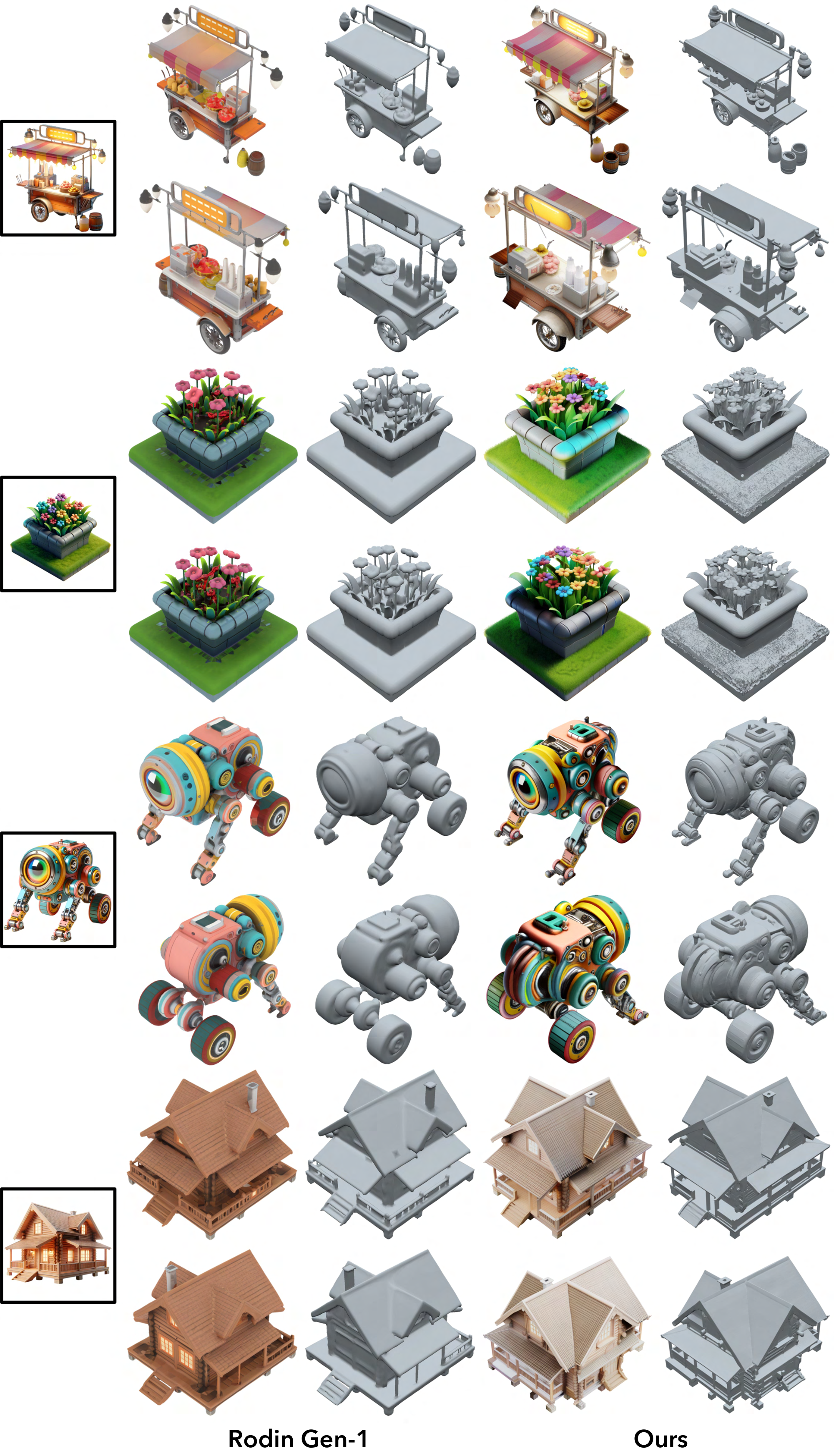
Figure 16 further compares our method with the commercial-level 3D generation model, Rodin Gen-1^2, using its default image-to-3D generation setting. Our method exhibits more detailed geometry structures on these complex cases, while being trained solely on open-source datasets and without commercial-specific designs.
D.3 3D Editing
Figure 17 and Figure 18 present additional editing results, highlighting the flexible capabilities of our method to edit and manipulate 3D assets.
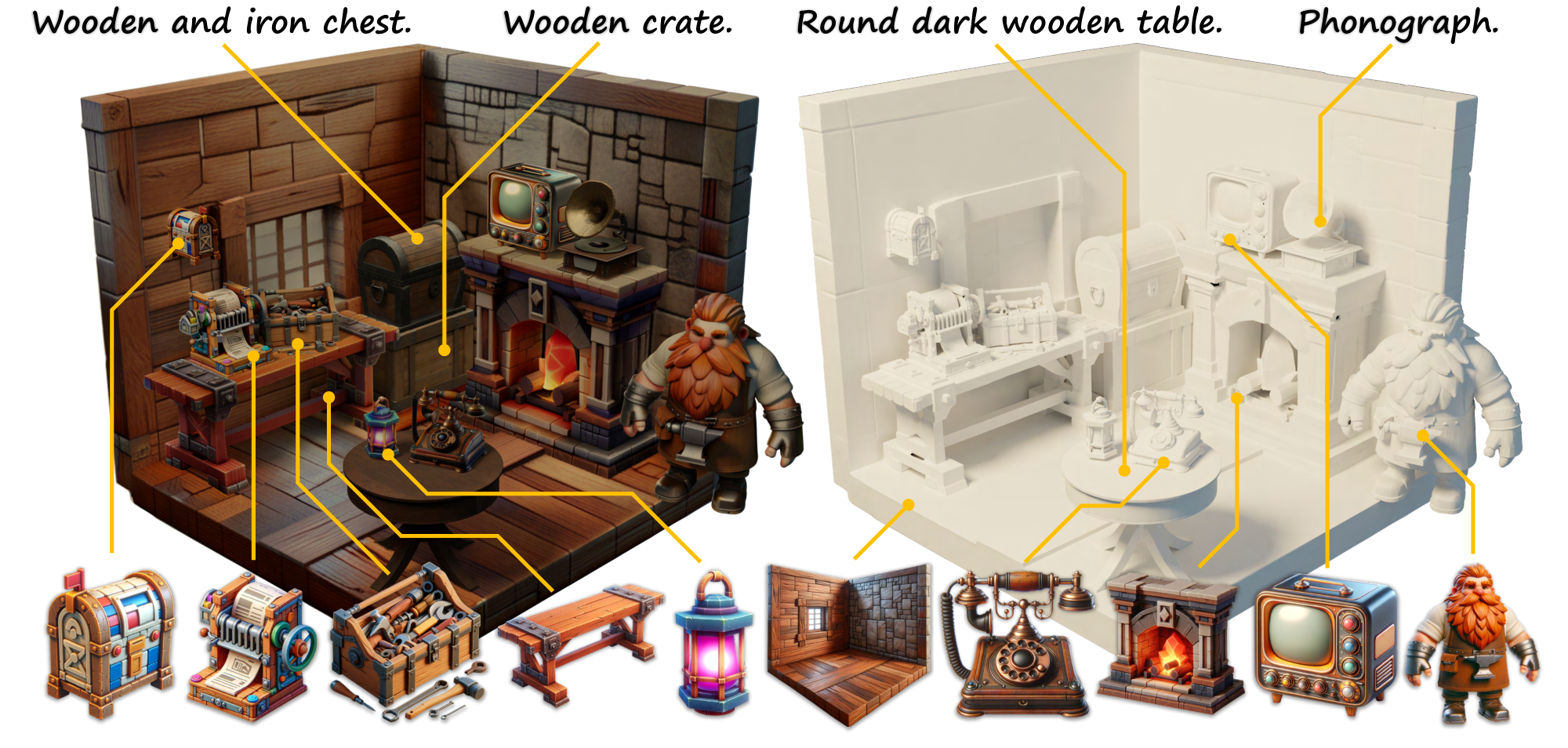
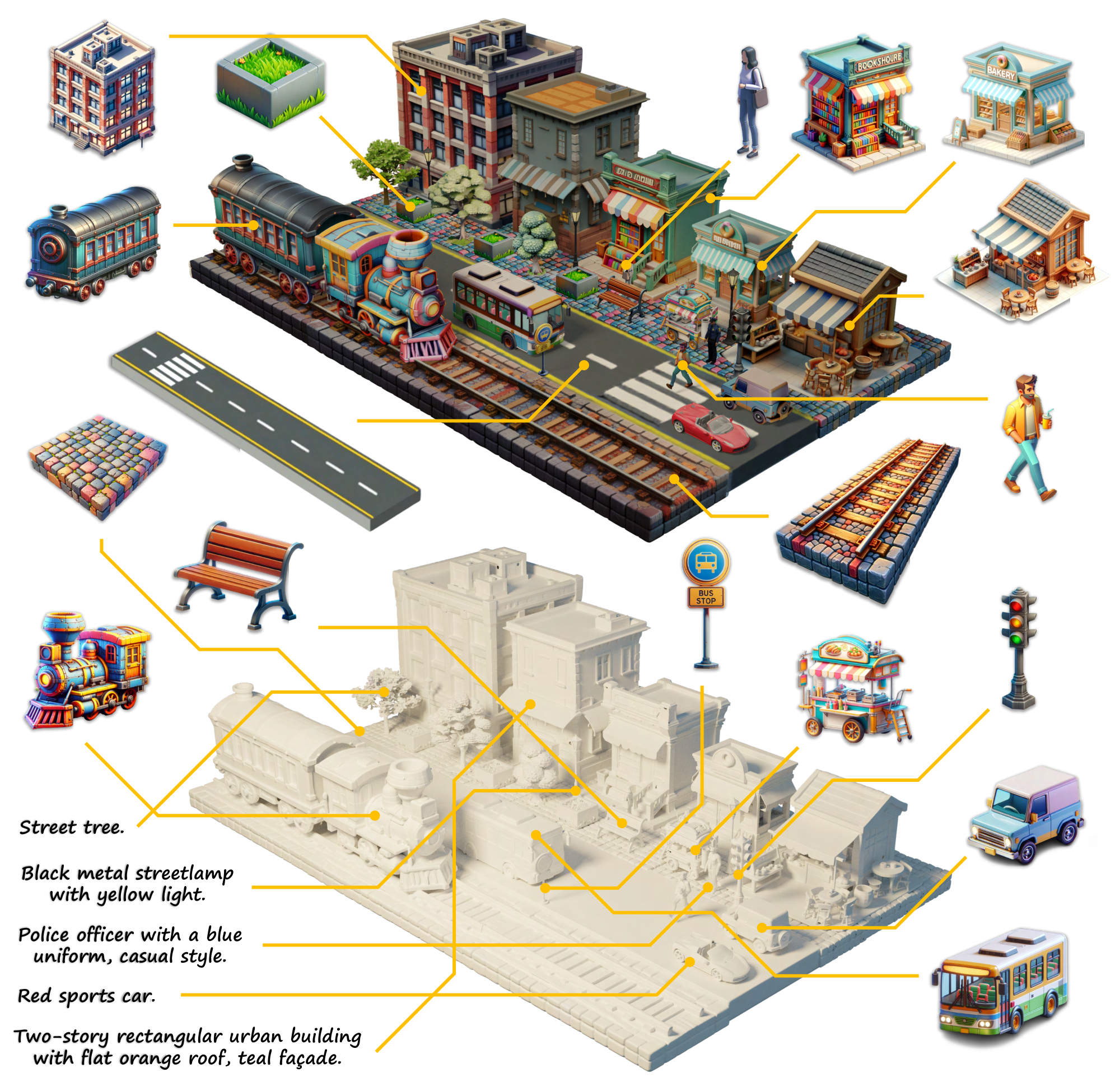
D.4 3D Scene Composition
Figure 19 and Figure 20 provide two supplementary visualizations of complex scenes constructed with assets from our model, demonstrating its potential for production use.
E. Limitations and Future works
While our model demonstrates strong performance on 3D generation, it still has some limitations. First, it uses a two-stage generation pipeline for the structured latent representation, which first generates the sparse structures, followed by the local latents on them. This approach can be less efficient than end-to-end methods that create complete 3D assets in a single stage.
Second, our image-to-3D model does not separate lighting effects in the generated 3D assets, resulting in baked-in shading and highlights from the reference image. A potential improvement is to apply more robust lighting augmentation for image prompts during training and enforce the model to predict materials for Physically Based Rendering (PBR), which we leave for future exploration.
References
Section Summary: This section compiles a list of academic papers and preprints that serve as foundational references for research on 3D content generation and reconstruction. The works focus on techniques such as text-to-3D synthesis via diffusion models, neural radiance fields for scene representation, and efficient rendering methods like Gaussian splatting. They also include advances in shape modeling, image synthesis, and scalable generative approaches for creating detailed 3D assets from limited inputs.
[1] Ben Poole, Ajay Jain, Jonathan T Barron, and Ben Mildenhall. Dreamfusion: Text-to-3d using 2d diffusion. In ICLR, 2023.
[2] Ruoshi Liu, Rundi Wu, Basile Van Hoorick, Pavel Tokmakov, Sergey Zakharov, and Carl Vondrick. Zero-1-to-3: Zero-shot one image to 3d object. In Proceedings of the IEEE/CVF international conference on computer vision, pages 9298–9309, 2023a.
[3] Dmitry Tochilkin, David Pankratz, Zexiang Liu, Zixuan Huang, Adam Letts, Yangguang Li, Ding Liang, Christian Laforte, Varun Jampani, and Yan-Pei Cao. Triposr: Fast 3d object reconstruction from a single image. arXiv preprint arXiv:2403.02151, 2024.
[4] Patrick Esser, Sumith Kulal, Andreas Blattmann, Rahim Entezari, Jonas Müller, Harry Saini, Yam Levi, Dominik Lorenz, Axel Sauer, Frederic Boesel, et al. Scaling rectified flow transformers for high-resolution image synthesis. In ICML, 2024.
[5] Junsong Chen, YU Jincheng, GE Chongjian, Lewei Yao, Enze Xie, Zhongdao Wang, James Kwok, Ping Luo, Huchuan Lu, and Zhenguo Li. Pixart- $\alpha$: Fast training of diffusion transformer for photorealistic text-to-image synthesis. In ICLR, 2024a.
[6] Ben Mildenhall, Pratul P Srinivasan, Matthew Tancik, Jonathan T Barron, Ravi Ramamoorthi, and Ren Ng. Nerf: Representing scenes as neural radiance fields for view synthesis. Communications of the ACM, 65(1):99–106, 2021.
[7] Bernhard Kerbl, Georgios Kopanas, Thomas Leimkühler, and George Drettakis. 3d gaussian splatting for real-time radiance field rendering. ACM Trans. Graph., 42(4):139–1, 2023.
[8] Yen-Chi Cheng, Hsin-Ying Lee, Sergey Tulyakov, Alexander G Schwing, and Liang-Yan Gui. Sdfusion: Multimodal 3d shape completion, reconstruction, and generation. In Proceedings of the IEEE/CVF Conference on Computer Vision and Pattern Recognition, pages 4456–4465, 2023.
[9] Anchit Gupta, Wenhan Xiong, Yixin Nie, Ian Jones, and Barlas Oğuz. 3dgen: Triplane latent diffusion for textured mesh generation. arXiv preprint arXiv:2303.05371, 2023.
[10] Yuhan Li, Yishun Dou, Xuanhong Chen, Bingbing Ni, Yilin Sun, Yutian Liu, and Fuzhen Wang. Generalized deep 3d shape prior via part-discretized diffusion process. In Proceedings of the IEEE/CVF Conference on Computer Vision and Pattern Recognition, pages 16784–16794, 2023.
[11] Xuanchi Ren, Jiahui Huang, Xiaohui Zeng, Ken Museth, Sanja Fidler, and Francis Williams. Xcube: Large-scale 3d generative modeling using sparse voxel hierarchies. In Proceedings of the IEEE/CVF Conference on Computer Vision and Pattern Recognition, pages 4209–4219, 2024.
[12] Bojun Xiong, Si-Tong Wei, Xin-Yang Zheng, Yan-Pei Cao, Zhouhui Lian, and Peng-Shuai Wang. Octfusion: Octree-based diffusion models for 3d shape generation. arXiv preprint arXiv:2408.14732, 2024.
[13] Biao Zhang, Jiapeng Tang, Matthias Niessner, and Peter Wonka. 3dshape2vecset: A 3d shape representation for neural fields and generative diffusion models. ACM Transactions on Graphics (TOG), 42(4):1–16, 2023.
[14] Longwen Zhang, Ziyu Wang, Qixuan Zhang, Qiwei Qiu, Anqi Pang, Haoran Jiang, Wei Yang, Lan Xu, and Jingyi Yu. Clay: A controllable large-scale generative model for creating high-quality 3d assets. ACM Transactions on Graphics (TOG), 43(4):1–20, 2024d.
[15] Lars Mescheder, Michael Oechsle, Michael Niemeyer, Sebastian Nowozin, and Andreas Geiger. Occupancy networks: Learning 3d reconstruction in function space. In Proceedings of the IEEE/CVF conference on computer vision and pattern recognition, pages 4460–4470, 2019.
[16] Jeong Joon Park, Peter Florence, Julian Straub, Richard Newcombe, and Steven Lovegrove. Deepsdf: Learning continuous signed distance functions for shape representation. In Proceedings of the IEEE/CVF conference on computer vision and pattern recognition, pages 165–174, 2019.
[17] Tengfei Wang, Bo Zhang, Ting Zhang, Shuyang Gu, Jianmin Bao, Tadas Baltrusaitis, Jingjing Shen, Dong Chen, Fang Wen, Qifeng Chen, et al. Rodin: A generative model for sculpting 3d digital avatars using diffusion. In Proceedings of the IEEE/CVF conference on computer vision and pattern recognition, pages 4563–4573, 2023.
[18] Yushi Lan, Fangzhou Hong, Shuai Yang, Shangchen Zhou, Xuyi Meng, Bo Dai, Xingang Pan, and Chen Change Loy. Ln3diff: Scalable latent neural fields diffusion for speedy 3d generation. In ECCV, 2024.
[19] Bowen Zhang, Yiji Cheng, Jiaolong Yang, Chunyu Wang, Feng Zhao, Yansong Tang, Dong Chen, and Baining Guo. Gaussiancube: Structuring gaussian splatting using optimal transport for 3d generative modeling. arXiv preprint arXiv:2403.19655, 2024b.
[20] Robin Rombach, Andreas Blattmann, Dominik Lorenz, Patrick Esser, and Björn Ommer. High-resolution image synthesis with latent diffusion models. In Proceedings of the IEEE/CVF conference on computer vision and pattern recognition, pages 10684–10695, 2022.
[21] Tao Lu, Mulin Yu, Linning Xu, Yuanbo Xiangli, Limin Wang, Dahua Lin, and Bo Dai. Scaffold-gs: Structured 3d gaussians for view-adaptive rendering. In Proceedings of the IEEE/CVF Conference on Computer Vision and Pattern Recognition, pages 20654–20664, 2024.
[22] Tianchang Shen, Jacob Munkberg, Jon Hasselgren, Kangxue Yin, Zian Wang, Wenzheng Chen, Zan Gojcic, Sanja Fidler, Nicholas Sharp, and Jun Gao. Flexible isosurface extraction for gradient-based mesh optimization. ACM Trans. Graph., 42(4), 2023.
[23] Quankai Gao, Qiangeng Xu, Hao Su, Ulrich Neumann, and Zexiang Xu. Strivec: Sparse tri-vector radiance fields. In Proceedings of the IEEE/CVF International Conference on Computer Vision, pages 17569–17579, 2023.
[24] Lingjie Liu, Jiatao Gu, Kyaw Zaw Lin, Tat-Seng Chua, and Christian Theobalt. Neural sparse voxel fields. Advances in Neural Information Processing Systems, 33:15651–15663, 2020.
[25] Maxime Oquab, Timothée Darcet, Théo Moutakanni, Huy V. Vo, Marc Szafraniec, Vasil Khalidov, Pierre Fernandez, Daniel HAZIZA, Francisco Massa, Alaaeldin El-Nouby, Mido Assran, Nicolas Ballas, Wojciech Galuba, Russell Howes, Po-Yao Huang, Shang-Wen Li, Ishan Misra, Michael Rabbat, Vasu Sharma, Gabriel Synnaeve, Hu Xu, Herve Jegou, Julien Mairal, Patrick Labatut, Armand Joulin, and Piotr Bojanowski. DINOv2: Learning robust visual features without supervision. Transactions on Machine Learning Research, 2024.
[26] Mohamed El Banani, Amit Raj, Kevis-Kokitsi Maninis, Abhishek Kar, Yuanzhen Li, Michael Rubinstein, Deqing Sun, Leonidas Guibas, Justin Johnson, and Varun Jampani. Probing the 3d awareness of visual foundation models. In Proceedings of the IEEE/CVF Conference on Computer Vision and Pattern Recognition, pages 21795–21806, 2024.
[27] Zi-Xin Zou, Zhipeng Yu, Yuan-Chen Guo, Yangguang Li, Ding Liang, Yan-Pei Cao, and Song-Hai Zhang. Triplane meets gaussian splatting: Fast and generalizable single-view 3d reconstruction with transformers. In Proceedings of the IEEE/CVF Conference on Computer Vision and Pattern Recognition, pages 10324–10335, 2024.
[28] Ian Goodfellow, Jean Pouget-Abadie, Mehdi Mirza, Bing Xu, David Warde-Farley, Sherjil Ozair, Aaron Courville, and Yoshua Bengio. Generative adversarial nets. Advances in Neural Information Processing Systems, 27, 2014.
[29] Jiajun Wu, Chengkai Zhang, Tianfan Xue, Bill Freeman, and Josh Tenenbaum. Learning a probabilistic latent space of object shapes via 3d generative-adversarial modeling. Advances in neural information processing systems, 29, 2016.
[30] Jun-Yan Zhu, Zhoutong Zhang, Chengkai Zhang, Jiajun Wu, Antonio Torralba, Josh Tenenbaum, and Bill Freeman. Visual object networks: Image generation with disentangled 3d representations. Advances in neural information processing systems, 31, 2018.
[31] Yu Deng, Jiaolong Yang, Jianfeng Xiang, and Xin Tong. Gram: Generative radiance manifolds for 3d-aware image generation. In IEEE/CVF International Conference on Computer Vision, 2022.
[32] Eric R Chan, Connor Z Lin, Matthew A Chan, Koki Nagano, Boxiao Pan, Shalini De Mello, Orazio Gallo, Leonidas Guibas, Jonathan Tremblay, Sameh Khamis, et al. Efficient geometry-aware 3d generative adversarial networks. In IEEE/CVF International Conference on Computer Vision, 2022.
[33] Jun Gao, Tianchang Shen, Zian Wang, Wenzheng Chen, Kangxue Yin, Daiqing Li, Or Litany, Zan Gojcic, and Sanja Fidler. Get3d: A generative model of high quality 3d textured shapes learned from images. Advances In Neural Information Processing Systems, 35:31841–31854, 2022.
[34] Ivan Skorokhodov, Aliaksandr Siarohin, Yinghao Xu, Jian Ren, Hsin-Ying Lee, Peter Wonka, and Sergey Tulyakov. 3d generation on imagenet. arXiv preprint arXiv:2303.01416, 2023.
[35] Xinyang Zheng, Yang Liu, Pengshuai Wang, and Xin Tong. Sdf-stylegan: Implicit sdf-based stylegan for 3d shape generation. In Computer Graphics Forum, pages 52–63, 2022.
[36] Jascha Sohl-Dickstein, Eric Weiss, Niru Maheswaranathan, and Surya Ganguli. Deep unsupervised learning using nonequilibrium thermodynamics. In International Conference on Machine Learning, pages 2256–2265. PMLR, 2015.
[37] Jonathan Ho, Ajay Jain, and Pieter Abbeel. Denoising diffusion probabilistic models. Advances in Neural Information Processing Systems, 33:6840–6851, 2020.
[38] Alex Nichol, Heewoo Jun, Prafulla Dhariwal, Pamela Mishkin, and Mark Chen. Point-e: A system for generating 3d point clouds from complex prompts. arXiv preprint arXiv:2212.08751, 2022.
[39] Shitong Luo and Wei Hu. Diffusion probabilistic models for 3d point cloud generation. In Proceedings of the IEEE/CVF conference on computer vision and pattern recognition, pages 2837–2845, 2021.
[40] Zhicong Tang, Shuyang Gu, Chunyu Wang, Ting Zhang, Jianmin Bao, Dong Chen, and Baining Guo. Volumediffusion: Flexible text-to-3d generation with efficient volumetric encoder. arXiv preprint arXiv:2312.11459, 2023b.
[41] Norman Müller, Yawar Siddiqui, Lorenzo Porzi, Samuel Rota Bulo, Peter Kontschieder, and Matthias Nießner. Diffrf: Rendering-guided 3d radiance field diffusion. In Proceedings of the IEEE/CVF Conference on Computer Vision and Pattern Recognition, pages 4328–4338, 2023.
[42] Ka-Hei Hui, Ruihui Li, Jingyu Hu, and Chi-Wing Fu. Neural wavelet-domain diffusion for 3d shape generation. In SIGGRAPH Asia 2022 Conference Papers, pages 1–9, 2022.
[43] Hansheng Chen, Jiatao Gu, Anpei Chen, Wei Tian, Zhuowen Tu, Lingjie Liu, and Hao Su. Single-stage diffusion nerf: A unified approach to 3d generation and reconstruction. In Proceedings of the IEEE/CVF international conference on computer vision, pages 2416–2425, 2023.
[44] J Ryan Shue, Eric Ryan Chan, Ryan Po, Zachary Ankner, Jiajun Wu, and Gordon Wetzstein. 3d neural field generation using triplane diffusion. In Proceedings of the IEEE/CVF Conference on Computer Vision and Pattern Recognition, pages 20875–20886, 2023.
[45] Bowen Zhang, Yiji Cheng, Chunyu Wang, Ting Zhang, Jiaolong Yang, Yansong Tang, Feng Zhao, Dong Chen, and Baining Guo. Rodinhd: High-fidelity 3d avatar generation with diffusion models. arXiv preprint arXiv:2407.06938, 2024a.
[46] Xianglong He, Junyi Chen, Sida Peng, Di Huang, Yangguang Li, Xiaoshui Huang, Chun Yuan, Wanli Ouyang, and Tong He. Gvgen: Text-to-3d generation with volumetric representation. In ECCV, 2024.
[47] Charlie Nash, Yaroslav Ganin, SM Ali Eslami, and Peter Battaglia. Polygen: An autoregressive generative model of 3d meshes. In International conference on machine learning, pages 7220–7229. PMLR, 2020.
[48] Yiwen Chen, Tong He, Di Huang, Weicai Ye, Sijin Chen, Jiaxiang Tang, Xin Chen, Zhongang Cai, Lei Yang, Gang Yu, et al. Meshanything: Artist-created mesh generation with autoregressive transformers. arXiv preprint arXiv:2406.10163, 2024b.
[49] Alec Radford, Jeffrey Wu, Rewon Child, David Luan, Dario Amodei, Ilya Sutskever, et al. Language models are unsupervised multitask learners. OpenAI blog, 1(8):9, 2019.
[50] Zibo Zhao, Wen Liu, Xin Chen, Xianfang Zeng, Rui Wang, Pei Cheng, Bin Fu, Tao Chen, Gang Yu, and Shenghua Gao. Michelangelo: Conditional 3d shape generation based on shape-image-text aligned latent representation. Advances in Neural Information Processing Systems, 36, 2024.
[51] Arash Vahdat, Francis Williams, Zan Gojcic, Or Litany, Sanja Fidler, Karsten Kreis, et al. Lion: Latent point diffusion models for 3d shape generation. Advances in Neural Information Processing Systems, 35:10021–10039, 2022.
[52] Weiyu Li, Jiarui Liu, Rui Chen, Yixun Liang, Xuelin Chen, Ping Tan, and Xiaoxiao Long. Craftsman: High-fidelity mesh generation with 3d native generation and interactive geometry refiner. arXiv preprint arXiv:2405.14979, 2024b.
[53] Shuang Wu, Youtian Lin, Feihu Zhang, Yifei Zeng, Jingxi Xu, Philip Torr, Xun Cao, and Yao Yao. Direct3d: Scalable image-to-3d generation via 3d latent diffusion transformer. arXiv preprint arXiv:2405.14832, 2024.
[54] Xin-Yang Zheng, Hao Pan, Peng-Shuai Wang, Xin Tong, Yang Liu, and Heung-Yeung Shum. Locally attentional sdf diffusion for controllable 3d shape generation. ACM Transactions on Graphics (ToG), 42(4):1–13, 2023.
[55] Heewoo Jun and Alex Nichol. Shap-e: Generating conditional 3d implicit functions. arXiv preprint arXiv:2305.02463, 2023.
[56] Evangelos Ntavelis, Aliaksandr Siarohin, Kyle Olszewski, Chaoyang Wang, Luc V Gool, and Sergey Tulyakov. Autodecoding latent 3d diffusion models. Advances in Neural Information Processing Systems, 36:67021–67047, 2023.
[57] Haitao Yang, Yuan Dong, Hanwen Jiang, Dejia Xu, Georgios Pavlakos, and Qixing Huang. Atlas gaussians diffusion for 3d generation with infinite number of points. arXiv preprint arXiv:2408.13055, 2024.
[58] Zhaoxi Chen, Jiaxiang Tang, Yuhao Dong, Ziang Cao, Fangzhou Hong, Yushi Lan, Tengfei Wang, Haozhe Xie, Tong Wu, Shunsuke Saito, et al. 3dtopia-xl: Scaling high-quality 3d asset generation via primitive diffusion. arXiv preprint arXiv:2409.12957, 2024c.
[59] Jiaxiang Tang, Jiawei Ren, Hang Zhou, Ziwei Liu, and Gang Zeng. Dreamgaussian: Generative gaussian splatting for efficient 3d content creation. In ICLR, 2024b.
[60] Chen-Hsuan Lin, Jun Gao, Luming Tang, Towaki Takikawa, Xiaohui Zeng, Xun Huang, Karsten Kreis, Sanja Fidler, Ming-Yu Liu, and Tsung-Yi Lin. Magic3d: High-resolution text-to-3d content creation. In Proceedings of the IEEE/CVF Conference on Computer Vision and Pattern Recognition, pages 300–309, 2023.
[61] Zhengyi Wang, Cheng Lu, Yikai Wang, Fan Bao, Chongxuan Li, Hang Su, and Jun Zhu. Prolificdreamer: High-fidelity and diverse text-to-3d generation with variational score distillation. Advances in Neural Information Processing Systems, 36, 2024.
[62] Junshu Tang, Tengfei Wang, Bo Zhang, Ting Zhang, Ran Yi, Lizhuang Ma, and Dong Chen. Make-it-3d: High-fidelity 3d creation from a single image with diffusion prior. In Proceedings of the IEEE/CVF international conference on computer vision, pages 22819–22829, 2023a.
[63] Yixun Liang, Xin Yang, Jiantao Lin, Haodong Li, Xiaogang Xu, and Yingcong Chen. Luciddreamer: Towards high-fidelity text-to-3d generation via interval score matching. In Proceedings of the IEEE/CVF Conference on Computer Vision and Pattern Recognition, pages 6517–6526, 2024.
[64] Yicong Hong, Kai Zhang, Jiuxiang Gu, Sai Bi, Yang Zhou, Difan Liu, Feng Liu, Kalyan Sunkavalli, Trung Bui, and Hao Tan. Lrm: Large reconstruction model for single image to 3d. In ICLR, 2024.
[65] Minghua Liu, Ruoxi Shi, Linghao Chen, Zhuoyang Zhang, Chao Xu, Xinyue Wei, Hansheng Chen, Chong Zeng, Jiayuan Gu, and Hao Su. One-2-3-45++: Fast single image to 3d objects with consistent multi-view generation and 3d diffusion. In Proceedings of the IEEE/CVF Conference on Computer Vision and Pattern Recognition, pages 10072–10083, 2024a.
[66] Jiahao Li, Hao Tan, Kai Zhang, Zexiang Xu, Fujun Luan, Yinghao Xu, Yicong Hong, Kalyan Sunkavalli, Greg Shakhnarovich, and Sai Bi. Instant3d: Fast text-to-3d with sparse-view generation and large reconstruction model. In ICLR, 2024a.
[67] Xiaoxiao Long, Yuan-Chen Guo, Cheng Lin, Yuan Liu, Zhiyang Dou, Lingjie Liu, Yuexin Ma, Song-Hai Zhang, Marc Habermann, Christian Theobalt, et al. Wonder3d: Single image to 3d using cross-domain diffusion. In Proceedings of the IEEE/CVF Conference on Computer Vision and Pattern Recognition, pages 9970–9980, 2024.
[68] Yichun Shi, Peng Wang, Jianglong Ye, Long Mai, Kejie Li, and Xiao Yang. Mvdream: Multi-view diffusion for 3d generation. In ICLR, 2024.
[69] Jiaxiang Tang, Zhaoxi Chen, Xiaokang Chen, Tengfei Wang, Gang Zeng, and Ziwei Liu. Lgm: Large multi-view gaussian model for high-resolution 3d content creation. In ECCV, 2024a.
[70] Kai Zhang, Sai Bi, Hao Tan, Yuanbo Xiangli, Nanxuan Zhao, Kalyan Sunkavalli, and Zexiang Xu. Gs-lrm: Large reconstruction model for 3d gaussian splatting. European Conference on Computer Vision, 2024c.
[71] Jianfeng Xiang, Jiaolong Yang, Binbin Huang, and Xin Tong. 3d-aware image generation using 2d diffusion models. In Proceedings of the IEEE/CVF International Conference on Computer Vision, pages 2383–2393, 2023.
[72] Minghua Liu, Chong Zeng, Xinyue Wei, Ruoxi Shi, Linghao Chen, Chao Xu, Mengqi Zhang, Zhaoning Wang, Xiaoshuai Zhang, Isabella Liu, et al. Meshformer: High-quality mesh generation with 3d-guided reconstruction model. arXiv preprint arXiv:2408.10198, 2024b.
[73] Xingchao Liu, Chengyue Gong, and Qiang Liu. Flow straight and fast: Learning to generate and transfer data with rectified flow. In ICLR, 2023b.
[74] Michael Samuel Albergo and Eric Vanden-Eijnden. Building normalizing flows with stochastic interpolants. In ICLR, 2023.
[75] Yaron Lipman, Ricky TQ Chen, Heli Ben-Hamu, Maximilian Nickel, and Matthew Le. Flow matching for generative modeling. In ICLR, 2023.
[76] The Movie Gen team. Movie gen: A cast of media foundation model. https://ai.meta.com/research/movie-gen/, 2024.
[77] Ze Liu, Yutong Lin, Yue Cao, Han Hu, Yixuan Wei, Zheng Zhang, Stephen Lin, and Baining Guo. Swin transformer: Hierarchical vision transformer using shifted windows. In Proceedings of the IEEE/CVF international conference on computer vision, pages 10012–10022, 2021.
[78] Yu-Qi Yang, Yu-Xiao Guo, Jian-Yu Xiong, Yang Liu, Hao Pan, Peng-Shuai Wang, Xin Tong, and Baining Guo. Swin3d: A pretrained transformer backbone for 3d indoor scene understanding, 2023.
[79] Richard Zhang, Phillip Isola, Alexei A Efros, Eli Shechtman, and Oliver Wang. The unreasonable effectiveness of deep features as a perceptual metric. In Proceedings of the IEEE conference on computer vision and pattern recognition, pages 586–595, 2018.
[80] William Peebles and Saining Xie. Scalable diffusion models with transformers. In Proceedings of the IEEE/CVF International Conference on Computer Vision, pages 4195–4205, 2023.
[81] Alec Radford, Jong Wook Kim, Chris Hallacy, Aditya Ramesh, Gabriel Goh, Sandhini Agarwal, Girish Sastry, Amanda Askell, Pamela Mishkin, Jack Clark, et al. Learning transferable visual models from natural language supervision. In International conference on machine learning, pages 8748–8763. PMLR, 2021.
[82] Peng-Shuai Wang, Yang Liu, Yu-Xiao Guo, Chun-Yu Sun, and Xin Tong. O-cnn: octree-based convolutional neural networks for 3d shape analysis. ACM Trans. Graph., 36(4), 2017.
[83] Andreas Lugmayr, Martin Danelljan, Andres Romero, Fisher Yu, Radu Timofte, and Luc Van Gool. Repaint: Inpainting using denoising diffusion probabilistic models. In Proceedings of the IEEE/CVF conference on computer vision and pattern recognition, pages 11461–11471, 2022.
[84] Matt Deitke, Ruoshi Liu, Matthew Wallingford, Huong Ngo, Oscar Michel, Aditya Kusupati, Alan Fan, Christian Laforte, Vikram Voleti, Samir Yitzhak Gadre, et al. Objaverse-xl: A universe of 10m+ 3d objects. Advances in Neural Information Processing Systems, 36, 2024.
[85] Jasmine Collins, Shubham Goel, Kenan Deng, Achleshwar Luthra, Leon Xu, Erhan Gundogdu, Xi Zhang, Tomas F Yago Vicente, Thomas Dideriksen, Himanshu Arora, et al. Abo: Dataset and benchmarks for real-world 3d object understanding. In Proceedings of the IEEE/CVF conference on computer vision and pattern recognition, pages 21126–21136, 2022.
[86] Huan Fu, Rongfei Jia, Lin Gao, Mingming Gong, Binqiang Zhao, Steve Maybank, and Dacheng Tao. 3d-future: 3d furniture shape with texture. International Journal of Computer Vision, pages 1–25, 2021.
[87] Mukul Khanna*, Yongsen Mao*, Hanxiao Jiang, Sanjay Haresh, Brennan Shacklett, Dhruv Batra, Alexander Clegg, Eric Undersander, Angel X. Chang, and Manolis Savva. Habitat Synthetic Scenes Dataset (HSSD-200): An Analysis of 3D Scene Scale and Realism Tradeoffs for ObjectGoal Navigation. arXiv preprint, 2023.
[88] Gpt-4o system card. 2024.
[89] Jonathan Ho and Tim Salimans. Classifier-free diffusion guidance. In NeurIPS 2021 Workshop on Deep Generative Models and Downstream Applications, 2021.
[90] I Loshchilov. Decoupled weight decay regularization. arXiv preprint arXiv:1711.05101, 2017.
[91] Stefan Stojanov, Anh Thai, and James M Rehg. Using shape to categorize: Low-shot learning with an explicit shape bias. In Proceedings of the IEEE/CVF conference on computer vision and pattern recognition, pages 1798–1808, 2021.
[92] Josh Achiam, Steven Adler, Sandhini Agarwal, Lama Ahmad, Ilge Akkaya, Florencia Leoni Aleman, Diogo Almeida, Janko Altenschmidt, Sam Altman, Shyamal Anadkat, et al. Gpt-4 technical report. arXiv preprint arXiv:2303.08774, 2023.
[93] James Betker, Gabriel Goh, Li Jing, Tim Brooks, Jianfeng Wang, Linjie Li, Long Ouyang, Juntang Zhuang, Joyce Lee, Yufei Guo, et al. Improving image generation with better captions. Computer Science. https://cdn. openai. com/papers/dall-e-3. pdf, 2(3):8, 2023.
[94] Jiale Xu, Weihao Cheng, Yiming Gao, Xintao Wang, Shenghua Gao, and Ying Shan. Instantmesh: Efficient 3d mesh generation from a single image with sparse-view large reconstruction models. arXiv preprint arXiv:2404.07191, 2024.
[95] Martin Heusel, Hubert Ramsauer, Thomas Unterthiner, Bernhard Nessler, and Sepp Hochreiter. Gans trained by a two time-scale update rule converge to a local nash equilibrium. Advances in neural information processing systems, 30, 2017.
[96] Mikołaj Bińkowski, Danica J Sutherland, Michael Arbel, and Arthur Gretton. Demystifying mmd gans. In International Conference on Learning Representations, 2018.
[97] Christian Szegedy, Vincent Vanhoucke, Sergey Ioffe, Jon Shlens, and Zbigniew Wojna. Rethinking the inception architecture for computer vision. In Proceedings of the IEEE conference on computer vision and pattern recognition, pages 2818–2826, 2016.
[98] Charles Ruizhongtai Qi, Li Yi, Hao Su, and Leonidas J Guibas. Pointnet++: Deep hierarchical feature learning on point sets in a metric space. Advances in neural information processing systems, 30, 2017.
[99] A Vaswani. Attention is all you need. Advances in Neural Information Processing Systems, 2017.
[100] Wenzhe Shi, Jose Caballero, Ferenc Huszár, Johannes Totz, Andrew P Aitken, Rob Bishop, Daniel Rueckert, and Zehan Wang. Real-time single image and video super-resolution using an efficient sub-pixel convolutional neural network. In Proceedings of the IEEE conference on computer vision and pattern recognition, pages 1874–1883, 2016.
[101] Tri Dao. Flashattention-2: Faster attention with better parallelism and work partitioning. In ICLR, 2024.
[102] Benjamin Lefaudeux, Francisco Massa, Diana Liskovich, Wenhan Xiong, Vittorio Caggiano, Sean Naren, Min Xu, Jieru Hu, Marta Tintore, Susan Zhang, Patrick Labatut, Daniel Haziza, Luca Wehrstedt, Jeremy Reizenstein, and Grigory Sizov. xformers: A modular and hackable transformer modelling library. https://github.com/facebookresearch/xformers, 2022.
[103] Biao Zhang and Rico Sennrich. Root mean square layer normalization. Advances in Neural Information Processing Systems, 32, 2019.
[104] Fausto Milletari, Nassir Navab, and Seyed-Ahmad Ahmadi. V-net: Fully convolutional neural networks for volumetric medical image segmentation. In 2016 fourth international conference on 3D vision (3DV), pages 565–571. Ieee, 2016.
[105] Zehao Yu, Anpei Chen, Binbin Huang, Torsten Sattler, and Andreas Geiger. Mip-splatting: Alias-free 3d gaussian splatting. In Proceedings of the IEEE/CVF Conference on Computer Vision and Pattern Recognition, pages 19447–19456, 2024.
[106] Stephen Lombardi, Tomas Simon, Gabriel Schwartz, Michael Zollhoefer, Yaser Sheikh, and Jason Saragih. Mixture of volumetric primitives for efficient neural rendering. ACM Transactions on Graphics (ToG), 40(4):1–13, 2021.
[107] Anpei Chen, Zexiang Xu, Andreas Geiger, Jingyi Yu, and Hao Su. Tensorf: Tensorial radiance fields. In European conference on computer vision, pages 333–350. Springer, 2022.
[108] Samuli Laine, Janne Hellsten, Tero Karras, Yeongho Seol, Jaakko Lehtinen, and Timo Aila. Modular primitives for high-performance differentiable rendering. ACM Transactions on Graphics (ToG), 39(6):1–14, 2020.
[109] Matt Deitke, Dustin Schwenk, Jordi Salvador, Luca Weihs, Oscar Michel, Eli VanderBilt, Ludwig Schmidt, Kiana Ehsani, Aniruddha Kembhavi, and Ali Farhadi. Objaverse: A universe of annotated 3d objects. In Proceedings of the IEEE/CVF Conference on Computer Vision and Pattern Recognition, pages 13142–13153, 2023.
[110] Tiange Luo, Chris Rockwell, Honglak Lee, and Justin Johnson. Scalable 3d captioning with pretrained models. Advances in Neural Information Processing Systems, 36, 2024.
[111] Yunhao Ge, Xiaohui Zeng, Jacob Samuel Huffman, Tsung-Yi Lin, Ming-Yu Liu, and Yin Cui. Visual fact checker: Enabling high-fidelity detailed caption generation. In Proceedings of the IEEE/CVF Conference on Computer Vision and Pattern Recognition, pages 14033–14042, 2024.
[112] Alexander Kirillov, Eric Mintun, Nikhila Ravi, Hanzi Mao, Chloe Rolland, Laura Gustafson, Tete Xiao, Spencer Whitehead, Alexander C Berg, Wan-Yen Lo, et al. Segment anything. In Proceedings of the IEEE/CVF International Conference on Computer Vision, pages 4015–4026, 2023.