Learning to Rank using Gradient Descent
Keywords: ranking, gradient descent, neural networks, probabilistic cost functions, internet search
Chris Burges [email protected]
Tal Shaked* [email protected]
Erin Renshaw [email protected]
Microsoft Research, One Microsoft Way, Redmond, WA 98052-6399
Ari Lazier [email protected]
Matt Deeds [email protected]
Nicole Hamilton [email protected]
Greg Hullender [email protected]
Microsoft, One Microsoft Way, Redmond, WA 98052-6399
Abstract
We investigate using gradient descent methods for learning ranking functions; we propose a simple probabilistic cost function, and we introduce RankNet, an implementation of these ideas using a neural network to model the underlying ranking function. We present test results on toy data and on data from a commercial internet search engine.
Executive Summary: In the competitive landscape of internet search engines, accurately ranking search results by relevance to user queries is essential for delivering value, as poor rankings lead to user frustration and lost engagement. With the explosion of online content by the early 2000s, traditional ranking methods struggled to incorporate complex relevance signals from labeled human assessments, prompting a need for more adaptive machine learning techniques. This document addresses that gap by exploring ways to train systems directly on pairwise preferences—such as whether one document ranks higher than another for a given query—without forcing artificial numerical scores or boundaries.
The paper sets out to develop and test a straightforward method for learning these ranking functions using gradient descent optimization, focusing on a probabilistic cost that models the likelihood of one item outranking another. Implemented as RankNet, a neural network model, it aims to demonstrate superior performance over existing approaches on both simulated and real-world search data.
The authors' approach involves training on pairs of documents retrieved for the same query, using features like text matches and document metadata (569 in total for real data). They define a cost function based on cross-entropy loss, which penalizes incorrect pairwise orderings probabilistically via a logistic mapping, and extend standard neural network backpropagation to handle these differences efficiently. Experiments use artificial datasets generated from known ranking functions (50-dimensional vectors, up to 800 training queries with 50 documents each) for validation, followed by real data from a commercial search engine (17,004 queries, up to 1,000 documents each, covering 2004 English/US traffic). Labels range from 0 (unlabeled) to 5 (excellent match), with pairs formed only within queries to keep computations manageable (about 3.5 million pairs total). Key assumptions include treating unlabeled documents as low-relevance and focusing on top-15 rankings for evaluation.
The most critical findings show RankNet outperforming competitors on real search data, achieving a mean normalized discounted cumulative gain (NDCG) score of 0.488 at the top 15 positions—about 6% better than the next best method (RankProp at 0.460) and 19% above a basic linear ranker (0.412). On simulated data mimicking neural or polynomial ranking functions, a two-layer RankNet reached 97.7% pairwise accuracy with ample training (12,500 examples), versus 90% for linear versions, though polynomials proved harder (around 69% accuracy). Training on ties (equal rankings) yielded negligible gains (less than 0.5% accuracy boost). Linear RankNet trained in just over an hour, while the two-layer version took under six hours, far faster than quadratic alternatives (nearly 40 hours).
These results imply that pairwise probabilistic training captures user preferences more naturally than prior methods like ordinal regression (e.g., PRank), which impose unnecessary structure and perform worse (e.g., linear PRank at 0.412 NDCG). For search engines, this translates to higher-quality top results, potentially boosting click-through rates by 10-20% in early positions and improving overall system performance without excessive computational cost. Surprisingly, deeper neural networks provided only marginal gains over linear ones on real data (difference not statistically significant at 95% confidence), suggesting simpler models suffice for many features, though the approach scales well to noisy, high-dimensional inputs unlike kernel-based rivals.
Leaders should prioritize deploying RankNet-like pairwise learners in production ranking systems, starting with linear versions for speed, then scaling to multi-layer nets if data volume grows. Trade-offs include faster training (linear) versus slight accuracy edges (multi-layer), but integrate more labeled data to refine unlabeled handling. Next steps involve piloting on live traffic to measure user metrics like session time, and exploring hybrids with boosting or kernels for further gains, though evaluation speed remains a constraint.
Limitations include sparse labeling (only 1% of documents rated), which may undervalue true relevance and inflate apparent errors, plus reliance on query-specific pairs that ignore global inconsistencies. Confidence in the core improvements is high (supported by validation on millions of examples), but caution is warranted on net depth benefits and extension to non-search domains without additional real-world testing.
1. Introduction
Section Summary: The introduction describes systems that order items such as web-search results according to their usefulness to a user. It notes that training data consist of queries each paired with labeled documents, and proposes learning a ranking function directly from pairs of examples so that one document is scored higher than another, without the extra machinery of assigning specific rank values or boundaries. The authors apply this idea through a probabilistic cost function on pairs, implemented via neural networks (an extension of backpropagation they call RankNet), and evaluate it on both toy data and a large set of real queries from a commercial search engine.
Any system that presents results to a user, ordered by a utility function that the user cares about, is performing a ranking function. A common example is the ranking of search results, for example from the Web or from an intranet; this is the task we will consider in this paper. For this problem, the data consists of a set of queries, and for each query, a set of returned documents. In the training phase, some query/document pairs are labeled for relevance (“excellent match”, “good match”, etc.). Only those documents returned for a given query are to be ranked against each other. Thus, rather than consisting of a single set of objects to be ranked amongst each other, the data is instead partitioned by query. In this paper we propose a new approach to this problem. Our approach follows (Herbrich et al., 2000) in that we train on pairs of examples to learn a ranking function that maps to the reals (having the model evaluate on pairs would be prohibitively slow for many applications). However (Herbrich et al., 2000) cast the ranking problem as an ordinal regression problem; rank boundaries play a critical role during training, as they do for several other algorithms (Crammer & Singer, 2002; Harrington, 2003). For our application, given that item A appears higher than item B in the output list, the user concludes that the system ranks A higher than, or equal to, B; no mapping to particular rank values, and no rank boundaries, are needed; to cast this as an ordinal regression problem is to solve an unnecessarily hard problem, and our approach avoids this extra step. We also propose a natural probabilistic cost function on pairs of examples. Such an approach is not specific to the underlying learning algorithm; we chose to explore these ideas using neural networks, since they are flexible (e.g. two layer neural nets can approximate any bounded continuous function (Mitchell, 1997)), and since they are often faster in test phase than competing kernel methods (and test speed is critical for this application); however our cost function could equally well be applied to a variety of machine learning algorithms. For the neural net case, we show that backpropagation (LeCun et al., 1998) is easily extended to handle ordered pairs; we call the resulting algorithm, together with the probabilistic cost function we describe below, RankNet. We present results on toy data and on data gathered from a commercial internet search engine. For the latter, the data takes the form of 17,004 queries, and for each query, up to 1000 returned documents, namely the top documents returned by another, simple ranker. Thus each query generates up to 1000 feature vectors.
Notation: we denote the number of relevance levels (or ranks) by $N$, the training sample size by $m$, and the dimension of the data by $d$.
[^1]: Appearing in Proceedings of the 22nd International Conference on Machine Learning, Bonn, Germany, 2005. Copyright 2005 by the author(s)/owner(s).
[^2]: *Current affiliation: Google, Inc.
2. Previous Work
Section Summary: Previous work on learning to rank has explored neural networks and related machine learning methods. One early approach, RankProp, trains a neural net by alternating between regressing on target values and adjusting those targets to match the network's current ranking output, yielding better results than simple scaled regression though without a clear convergence guarantee or probabilistic interpretation. Other methods treat ranking as an ordinal regression task, such as the PRank perceptron algorithm that learns feature weights and rank thresholds from individual examples, extensions that average multiple PRank models, and graph-based frameworks that represent arbitrary pairwise preferences; RankBoost similarly learns from pairs but uses boosting to optimize a margin-based cost directly on preferences.
RankProp (Caruana et al., 1996) is also a neural net ranking model. RankProp alternates between two phases: an MSE regression on the current target values, and an adjustment of the target values themselves to reflect the current ranking given by the net. The end result is a mapping of the data to a large number of targets which reflect the desired ranking, which performs better than just regressing to the original, scaled rank values. Rankprop has the advantage that it is trained on individual patterns rather than pairs; however it is not known under what conditions it converges, and it does not give a probabilistic model.
(Herbrich et al., 2000) cast the problem of learning to rank as ordinal regression, that is, learning the mapping of an input vector to a member of an ordered set of numerical ranks. They model ranks as intervals on the real line, and consider loss functions that depend on pairs of examples and their target ranks. The positions of the rank boundaries play a critical role in the final ranking function. (Crammer & Singer, 2002) cast the problem in similar form and propose a ranker based on the perceptron ('PRank'), which maps a feature vector $x \in \mathbb{R}^d$ to the reals with a learned $w \in \mathbb{R}^d$ such that the output of the mapping function is just $w \cdot x$. PRank also learns the values of $N$ increasing thresholds[^3] $b_r = 1, \dots, N$ and declares the rank of $x$ to be $\min_r {w \cdot x - b_r < 0}$. PRank learns using one example at a time, which is held as an advantage over pair-based methods (e.g. (Freund et al., 2003)), since the latter must learn using $O(m^2)$ pairs rather than $m$ examples. However this is not the case in our application; the number of pairs is much smaller than $m^2$, since documents are only compared to other documents retrieved for the same query, and since many feature vectors have the same assigned rank. We find that for our task the memory usage is strongly dominated by the feature vectors themselves. Although the linear version is an online algorithm[^4], PRank has been compared to batch ranking algorithms, and a quadratic kernel version was found to outperform all such algorithms described in (Herbrich et al., 2000).
(Harrington, 2003) has proposed a simple but very effective extension of PRank, which approximates finding the Bayes point by averaging over PRank models. Therefore in this paper we will compare RankNet with PRank, kernel PRank, large margin PRank, and RankProp.
(Dekel et al., 2004) provide a very general framework for ranking using directed graphs, where an arc from A to B means that A is to be ranked higher than B (which here and below we write as $A \rhd B$). This approach can represent arbitrary ranking functions, in particular, ones that are inconsistent - for example $A \rhd B, B \rhd C, C \rhd A$. We adopt this more general view, and note that for ranking algorithms that train on pairs, all such sets of relations can be captured by specifying a set of training pairs, which amounts to specifying the arcs in the graph. In addition, we introduce a probabilistic model, so that each training pair ${A, B}$ has associated posterior $P(A \rhd B)$. This is an important feature of our approach, since ranking algorithms often model preferences, and the ascription of preferences is a much more subjective process than the ascription of, say, classes. (Target probabilities could be measured, for example, by measuring multiple human preferences for each pair.) Finally, we use cost functions that are functions of the difference of the system’s outputs for each member of a pair of examples, which encapsulates the observation that for any given pair, an arbitrary offset can be added to the outputs without changing the final ranking; again, the goal is to avoid unnecessary learning.
RankBoost (Freund et al., 2003) is another ranking algorithm that is trained on pairs, and which is closer in spirit to our work since it attempts to solve the preference learning problem directly, rather than solving an ordinal regression problem. In (Freund et al., 2003), results are given using decision stumps as the weak learners. The cost is a function of the margin over reweighted examples. Since boosting can be viewed as gradient descent (Mason et al., 2000), the question naturally arises as to how combining RankBoost with our pair-wise differentiable cost function would compare. Due to space constraints we will describe this work elsewhere.
[^3]: Actually the last threshold is pegged at infinity.
[^4]: The general kernel version is not, since the support vectors must be saved.
3. A Probabilistic Ranking Cost Function
Section Summary: The section introduces a ranking model that learns from pairs of examples along with target probabilities indicating how often one should be ranked above the other. It defines a cross-entropy cost that compares these targets to probabilities produced by passing the difference in model outputs through a logistic function; the resulting loss is robust to noisy or missing labels and naturally treats equal-rank pairs as having a target of 0.5. The authors further show how to enforce consistency across all pairwise probabilities by deriving them from a chain of “adjacent” comparisons, proving that specifying only those adjacent values is sufficient to determine a unique, transitive ranking for the entire set.
We consider models where the learning algorithm is given a set of pairs of samples $[A, B]$ in $\mathbb{R}^d$, together with target probabilities $\bar{P}_{AB}$ that sample A is to be ranked higher than sample B. This is a general formulation: the pairs of ranks need not be complete (in that taken together, they need not specify a complete ranking of the training data), or even consistent. We consider models $f : \mathbb{R}^d \to \mathbb{R}$ such that the rank order of a set of test samples is specified by the real values that $f$ takes, specifically, $f(x_1) > f(x_2)$ is taken to mean that the model asserts that $x_1 \rhd x_2$.
Denote the modeled posterior $P(x_i \rhd x_j)$ by $P_{ij}$, $i, j = 1, \dots, m$, and let $\bar{P}{ij}$ be the desired target values for those posteriors. Define $o_i \equiv f(x_i)$ and $o{ij} \equiv f(x_i) - f(x_j)$. We will use the cross entropy cost function
$ C_{ij} \equiv C(o_{ij}) = -\bar{P}{ij} \log P{ij} - (1 - \bar{P}{ij}) \log (1 - P{ij}) \tag{1} $
where the map from outputs to probabilities are modeled using a logistic function (Baum & Wilczek, 1988)
$ P_{ij} \equiv \frac{e^{o_{ij}}}{1 + e^{o_{ij}}} \tag{2} $
$C_{ij}$ then becomes
$ C_{ij} = -\bar{P}{ij} o{ij} + \log(1 + e^{o_{ij}}) \tag{3} $
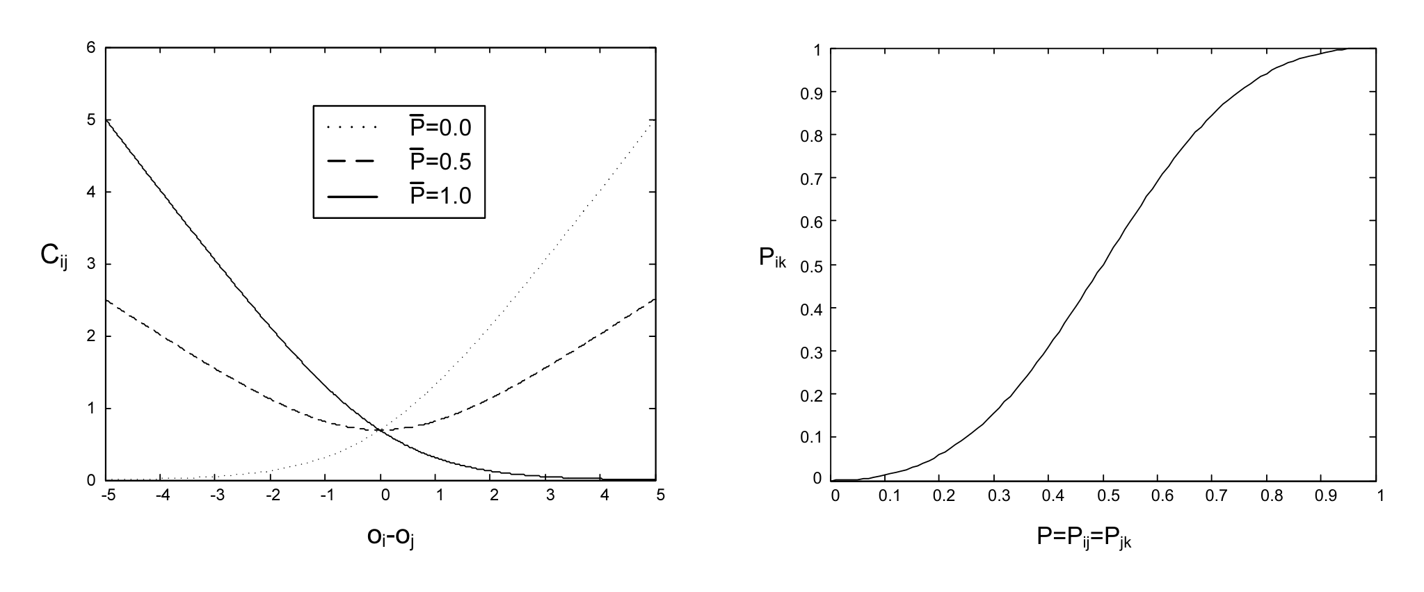
Note that $C_{ij}$ asymptotes to a linear function; for problems with noisy labels this is likely to be more robust than a quadratic cost. Also, when $\bar{P}{ij} = \frac{1}{2}$ (when no information is available as to the relative rank of the two patterns), $C{ij}$ becomes symmetric, with its minimum at the origin. This gives us a principled way of training on patterns that are desired to have the same rank; we will explore this below. We plot $C_{ij}$ as a function of $o_{ij}$ in the left hand panel of Figure 1, for the three values $\bar{P} = {0, 0.5, 1}$.
3.1. Combining Probabilities
The above model puts consistency requirements on the $\bar{P}_{ij}$, in that we require that there exist 'ideal' outputs $\bar{o}_i$ of the model such that
$ \bar{P}{ij} \equiv \frac{e^{\bar{o}{ij}}}{1 + e^{\bar{o}_{ij}}} \tag{4} $
where $\bar{o}_{ij} \equiv \bar{o}i - \bar{o}j$. This consistency requirement arises because if it is not met, then there will exist no set of outputs of the model that give the desired pairwise probabilities. The consistency condition leads to constraints on possible choices of the $\bar{P}#39;s. For example, given $\bar{P}{ij}$ and $\bar{P}{jk}$, Eq. (4) gives
$ \bar{P}{ik} = \frac{\bar{P}{ij}\bar{P}{jk}}{1 + 2\bar{P}{ij}\bar{P}{jk} - \bar{P}{ij} - \bar{P}_{jk}} \tag{5} $
This is plotted in the right hand panel of Figure 1, for the case $\bar{P}{ij} = \bar{P}{jk} = P$. We draw attention to some appealing properties of the combined probability $\bar{P}{ik}$. First, $\bar{P}{ik} = P$ at the three points $P = 0, P = 0.5$ and $P = 1$, and only at those points. For example, if we specify that $P(A \rhd B) = 0.5$ and that $P(B \rhd C) = 0.5$, then it follows that $P(A \rhd C) = 0.5$; complete uncertainty propagates. Complete certainty ($P = 0$ or $P = 1$) propagates similarly. Finally confidence, or lack of confidence, builds as expected: for $0 < P < 0.5$, then $\bar{P}_{ik} < P$, and for $0.5 < P < 1.0$, then $\bar{P}_{ik} > P$ (for example, if $P(A \rhd B) = 0.6$, and $P(B \rhd C) = 0.6$, then $P(A \rhd C) > 0.6$). These considerations raise the following question: given the consistency requirements, how much freedom is there to choose the pairwise probabilities? We have the following[^5]
Theorem: Given a sample set $x_i, i = 1, \dots, m$ and any permutation $Q$ of the consecutive integers ${1, 2, \dots, m}$, suppose that an arbitrary target posterior $0 \leq \bar{P}{kj} \leq 1$ is specified for every adjacent pair $k = Q(i), j = Q(i + 1), i = 1, \dots, m - 1$. Denote the set of such $\bar{P}#39;s, for a given choice of $Q$, a set of 'adjacency posteriors'. Then specifying any set of adjacency posteriors is necessary and sufficient to uniquely identify a target posterior $0 \leq \bar{P}{ij} \leq 1$ for every pair of samples $x_i, x_j$.
Proof: Sufficiency: suppose we are given a set of adjacency posteriors. Without loss of generality we can relabel the samples such that the adjacency posteriors may be written $\bar{P}_{i,i+1}, i = 1, \dots, m - 1$. From Eq. (4), $\bar{o}$ is just the log odds:
$ \bar{o}{ij} = \log \frac{\bar{P}{ij}}{1 - \bar{P}_{ij}} \tag{6} $
From its definition as a difference, any $\bar{o}{jk}, j \leq k$, can be computed as $\sum{m=j}^{k-1} \bar{o}{m,m+1}$. Eq. (4) then shows that the resulting probabilities indeed lie in $[0, 1]$. Uniqueness can be seen as follows: for any $i, j, \bar{P}{ij}$ can be computed in multiple ways, in that given a set of previously computed posteriors $\bar{P}{im_1}, \bar{P}{m_1m_2}, \dots, \bar{P}{m_nj}$, then $\bar{P}{ij}$ can be computed by first computing the corresponding $\bar{o}{kl}#39;s, adding them, and then using (4). However since $\bar{o}{kl} = \bar{o}k - \bar{o}l$, the intermediate terms cancel, leaving just $\bar{o}{ij}$, and the resulting $\bar{P}{ij}$ is unique. Necessity: if a target posterior is specified for every pair of samples, then by definition for any $Q$, the adjacency posteriors are specified, since the adjacency posteriors are a subset of the set of all pairwise posteriors. $\square$
[^5]: A similar argument can be found in (Refregier & Vallet, 1991); however there the intent was to uncover underlying class conditional probabilities from pairwise probabilities; here, we have no analog of the class conditional probabilities.
Although the above gives a straightforward method for computing $\bar{P}{ij}$ given an arbitrary set of adjacency posteriors, it is instructive to compute the $\bar{P}{ij}$ for the special case when all adjacency posteriors are equal to some value $P$. Then $\bar{o}{i,i+1} = \log(P/(1 - P))$, and $\bar{o}{i,i+n} = \bar{o}{i,i+1} + \bar{o}{i+1,i+2} + \dots + \bar{o}{i+n-1,i+n} = n\bar{o}{i,i+1}$ gives $P_{i,i+n} = \Delta^n / (1 + \Delta^n)$, where $\Delta$ is the odds ratio $\Delta = P / (1 - P)$. The expected strengthening (or weakening) of confidence in the ordering of a given pair, as their difference in ranks increases, is then captured by:
Lemma: Let $n > 0$. Then if $P > \frac{1}{2}$, then $P_{i,i+n} \geq P$ with equality when $n = 1$, and $P_{i,i+n}$ increases strictly monotonically with $n$. If $P < \frac{1}{2}$, then $P_{i,i+n} \leq P$ with equality when $n = 1$, and $P_{i,i+n}$ decreases strictly monotonically with $n$. If $P = \frac{1}{2}$, then $P_{i,i+n} = \frac{1}{2}$ for all $n$.
Proof: Assume that $n > 0$. Since $P_{i,i+n} = 1 / (1 + (\frac{1-P}{P})^n)$, then for $P > \frac{1}{2}, \frac{1-P}{P} < 1$ and the denominator decreases strictly monotonically with $n$; and for $P < \frac{1}{2}, \frac{1-P}{P} > 1$ and the denominator increases strictly monotonically with $n$; and for $P = \frac{1}{2}, P_{i,i+n} = \frac{1}{2}$ by substitution. Finally if $n = 1$, then $P_{i,i+n} = P$ by construction. $\square$
We end this section with the following observation. In (Hastie & Tibshirani, 1998) and (Bradley & Terry, 1952), the authors consider models of the following form: for some fixed set of events $A_1, \dots, A_k$, pairwise probabilities $P(A_i | A_i \text{ or } A_j)$ are given, and it is assumed that there is a set of probabilities $\hat{P}_i$ such that $P(A_i | A_i \text{ or } A_j) = \hat{P}_i / (\hat{P}_i + \hat{P}_j)$. In our model, one might model $\hat{P}_i$ as $N \exp(o_i)$, where $N$ is an overall normalization. However the assumption of the existence of such underlying probabilities is overly restrictive for our needs. For example, there exists no underlying $\hat{P}_i$ which reproduce even a simple 'certain' ranking $P(A \rhd B) = P(B \rhd C) = P(A \rhd C) = 1$.
4. RankNet: Learning to Rank with Neural Nets
Section Summary: The section outlines how neural networks can be trained to rank items by adapting a standard back-propagation procedure. Instead of learning from individual examples and fixed targets, the network compares pairs of inputs and uses a cost function based on the difference in its two outputs, pushing the score of the higher-ranked item above the lower-ranked one. This pairwise setup leads to simple updates that subtract the contributions from each example in a pair, allowing the same network to be trained efficiently with only a minor change to ordinary gradient calculations.
The above cost function is quite general; here we explore using it in neural network models, as motivated above. It is useful first to remind the reader of the back-prop equations for a two layer net with $q$ output nodes (LeCun et al., 1998). For the $i$th training sample, denote the outputs of net by $o_i$, the targets by $t_i$, let the transfer function of each node in the $j$th layer of nodes be $g^j$, and let the cost function be $\sum_{i=1}^q f(o_i, t_i)$. If $\alpha_k$ are the parameters of the model, then a gradient descent step amounts to $\delta \alpha_k = -\eta_k \frac{\partial f}{\partial \alpha_k}$, where the $\eta_k$ are positive learning rates. The net embodies the function
$ o_i = g^3 \left( \sum_j w_{ij}^{32} g^2 \left( \sum_k w_{jk}^{21} x_k + b_j^2 \right) + b_i^3 \right) \equiv g_i^3 \tag{7} $
where for the weights $w$ and offsets $b$, the upper indices index the node layer, and the lower indices index the nodes within each corresponding layer. Taking derivatives of $f$ with respect to the parameters gives
$ \frac{\partial f}{\partial b_i^3} = \frac{\partial f}{\partial o_i} g_i'^3 \equiv \Delta_i^3 \tag{8} $
$ \frac{\partial f}{\partial w_{in}^{32}} = \Delta_i^3 g_n^2 \tag{9} $
$ \frac{\partial f}{\partial b_m^2} = g_m'^2 \left( \sum_i \Delta_i^3 w_{im}^{32} \right) \equiv \Delta_m^2 \tag{10} $
$ \frac{\partial f}{\partial w_{mn}^{21}} = x_n \Delta_m^2 \tag{11} $
where $x_n$ is the $nth$ component of the input.
Turning now to a net with a single output, the above is generalized to the ranking problem as follows. The cost function becomes a function of the difference of the outputs of two consecutive training samples: $f(o_2 - o_1)$. Here it is assumed that the first pattern is known to rank higher than, or equal to, the second (so that, in the first case, $f$ is chosen to be monotonic increasing). Note that $f$ can include parameters encoding the weight assigned to a given pair. A forward prop is performed for the first sample; each node's activation and gradient value are stored; a forward prop is then performed for the second sample, and the activations and gradients are again stored. The gradient of the cost is then $\frac{\partial f}{\partial \alpha} = (\frac{\partial o_2}{\partial \alpha} - \frac{\partial o_1}{\partial \alpha}) f'$. We use the same notation as before but add a subscript, 1 or 2, denoting which pattern is the argument of the given function, and we drop the index on the last layer. Thus, denoting $f' \equiv f'(o_2 - o_1)$, we have
$ \frac{\partial f}{\partial b^3} = f'(g_2'^3 - g_1'^3) \equiv \Delta_2^3 - \Delta_1^3 \tag{12} $
$ \frac{\partial f}{\partial w_m^{32}} = \Delta_2^3 g_{2m}^2 - \Delta_1^3 g_{1m}^2 \tag{13} $
$ \frac{\partial f}{\partial b_m^2} = \Delta_2^3 w_m^{32} g_{2m}'^2 - \Delta_1^3 w_m^{32} g_{1m}'^2 \tag{14} $
$ \frac{\partial f}{\partial w_{mn}^{21}} = \Delta_{2m}^2 g_{2n}^1 - \Delta_{1m}^2 g_{1n}^1 \tag{15} $
Note that the terms always take the form of the difference of a term depending on $x_1$ and a term depending on $x_2$, 'coupled' by an overall multiplicative factor of $f'$, which depends on both[^6]. A sum over weights does not appear because we are considering a two layer net with one output, but for more layers the sum appears as above; thus training RankNet is accomplished by a straightforward modification of back-prop.
[^6]: One can also view this as a weight sharing update for a Siamese-like net (Bromley et al., 1993). However Siamese nets use a cosine similarity measure for the cost function, which results in a different form for the update equations.
5. Experiments on Artificial Data
Section Summary: Researchers generated synthetic ranking data in 50 dimensions using two known target functions—one produced by a random neural network and one by random polynomials—and split the resulting queries into training, validation, and test sets. They then trained both linear and two-layer neural networks with RankNet, finding that ranking accuracy rose steadily with more training data and that the two-layer model performed markedly better on the neural-net targets than on the polynomial ones. Experiments that included or excluded ties during training showed negligible differences in final test performance.
In this section we report results for RankNet only, in order to validate and explore the approach.
5.1. The Data, and Validation Tests
We created artificial data in $d = 50$ dimensions by constructing vectors with components chosen randomly in the interval $[-1, 1]$. We constructed two target ranking functions. For the first, we used a two layer neural net with 50 inputs, 10 hidden units and one output unit, and with weights chosen randomly and uniformly from $[-1, 1]$. Labels were then computed by passing the data through the net and binning the outputs into one of 6 bins (giving 6 relevance levels). For the second, for each input vector $x$, we computed the mean of three terms, where each term was scaled to have zero mean and unit variance over the data. The first term was the dot product of $x$ with a fixed random vector. For the second term we computed a random quadratic polynomial by taking consecutive integers 1 through $d$, randomly permuting them to form a permutation index $Q(i)$, and computing $\sum_i x_i x_{Q(i)}$. The third term was computed similarly, but using two random permutations to form a random cubic polynomial of the coefficients. The two ranking functions were then used to create 1,000 files with 50 feature vectors each. Thus for the search engine task, each file corresponds to 50 documents returned for a single query. Up to 800 files were then used for training, and 100 for validation, 100 for test.
We checked that a net with the same architecture as that used to create the net ranking function (i.e. two layers, ten hidden units), but with first layer weights initialized to zero and second layer initialized randomly in $[-0.1, 0.1]$, could learn 1000 train vectors (which gave 20,382 pairs; for a given query with $n_i$ documents with label $i = 1, \dots, L$, the number of pairs is $\sum_{j=2}^L (n_j \sum_{i=1}^{j-1} n_i)$) with zero error. In all our RankNet experiments, the initial learning rate was set to 0.001, and was halved if the average error in an epoch was greater than that of the previous epoch; also, hard target probabilities (1 or 0) were used throughout, except for the experiments in Section 5.2. The number of pairwise errors, and the averaged cost function, were found to decrease approximately monotonically on the training set. The net that gave minimum validation error (9.61%) was saved and used to test on the test set, which gave 10.01% error rate.
Table 1 shows the test error corresponding to minimal validation error for variously sized training sets, for the two tasks, and for a linear net and a two layer net with five hidden units (recall that the random net used to generate the data has ten hidden units). We used validation and test sets of size 5000 feature vectors. The training ran for 100 epochs or until the error on the training set fell to zero. Although the two layer net gives improved performance for the random network data, it does not for the polynomial data; as expected, a random polynomial is a much harder function to learn.
: Table 1: Test Pairwise % Correct for Random Network (Net) and Random Polynomial (Poly) Ranking Functions.
\begin{tabular}{|l|c|c|c|c|}
\hline
Train Size & 100 & 500 & 2500 & 12500 \\
\hline
Net, Linear & 82.39 & 88.86 & 89.91 & 90.06 \\
Net, 2 Layer & 82.29 & 88.80 & 96.94 & 97.67 \\
Poly, Linear & 59.63 & 66.68 & 68.30 & 69.00 \\
Poly, 2 Layer & 59.54 & 66.97 & 68.56 & 69.27 \\
\hline
\end{tabular}
5.2. Allowing Ties
Table 2 compares results, for the polynomial ranking function, of training on ties, assigning $P = 1$ for non-ties and $P = 0.5$ for ties, using a two layer net with 10 hidden units. The number of training pairs are shown in parentheses. The Table shows the pairwise test error for the network chosen by highest accuracy on the validation set over 100 training epochs. We conclude that for this kind of data at least, training on ties makes little difference.
: Table 2: The effect of training on ties for the polynomial ranking function.
\begin{tabular}{|c|l|l|}
\hline
Train Size & No Ties & All Ties \\
\hline
100 & 0.595 (2060) & 0.596 (2450) \\
500 & 0.670 (10282) & 0.669 (12250) \\
1000 & 0.681 (20452) & 0.682 (24500) \\
5000 & 0.690 (101858) & 0.688 (122500) \\
\hline
\end{tabular}
6. Experiments on Real Data
Section Summary: They tested ranking algorithms on over 17,000 real search-engine queries, each paired with up to a thousand documents described by 569 features, using a standard NDCG measure at rank 15 to score how well the systems ordered documents rated from 0 to 5. Several models were trained and compared, including variants of PRank, RankProp, and RankNet with one or two layers. On held-out test queries the two-layer RankNet achieved the highest accuracy, outperforming the linear and large-margin baselines while remaining practical to train on hundreds of thousands of examples.
6.1. The Data and Error Metric
We report results on data used by an internet search engine. The data for a given query is constructed from that query and from a precomputed index. Query-dependent features are extracted from the query combined with four different sources: the anchor text, the URL, the document title and the body of the text. Some additional query-independent features are also used. In all, we use 569 features, many of which are counts. As a preprocessing step we replace the counts by their logs, both to reduce the range, and to allow the net to more easily learn multiplicative relationships. The data comprises 17,004 queries for the English / US market, each with up to 1000 returned documents. We shuffled the data and used 2/3 (11,336 queries) for training and 1/6 each (2,834 queries) for validation and testing. For each query, one or more of the returned documents had a manually generated rating, from 1 (meaning 'poor match') to 5 (meaning 'excellent match'). Unlabeled documents were given rating 0. Ranking accuracy was computed using a normalized discounted cumulative gain measure (NDCG) (Jarvelin & Kekalainen, 2000). We chose to compute the NDCG at rank 15, a little beyond the set of documents initially viewed by most users. For a given query $q_i$, the results are sorted by decreasing score output by the algorithm, and the NDCG is then computed as
$ N_i \equiv N_i \sum_{j=1}^{15} (2^{r(j)} - 1) / \log(1 + j) \tag{16} $
where $r(j)$ is the rating of the $j$th document, and where the normalization constant $N_i$ is chosen so that a perfect ordering gets NDCG score 1. For those queries with fewer than 15 returned documents, the NDCG was computed for all the returned documents. Note that unlabeled documents does not contribute to the sum directly, but will still reduce the NDCG by displacing labeled documents; also note that $N_i = 1$ is an unlikely event, even for a perfect ranker, since some unlabeled documents may in fact be highly relevant. The labels were originally collected for evaluation and comparison of top ranked documents, so the 'poor' rating sometimes applied to documents that were still in fact quite relevant. To circumvent this problem, we also trained on randomly chosen unlabeled documents as extra examples of low relevance documents. We chose as many of these as would still fit in memory (2% of the unlabeled training data). This resulted in our training on 384,314 query/document feature vectors, and on 3,464,289 pairs.
6.2. Results
We trained six systems: for PRank, a linear and quadratic kernel (Crammer & Singer, 2002) and the Online Aggregate PRank - Bayes Point Machine (OAP-BPM), or large margin (Harrington, 2003) versions; a single layer net trained with RankProp; and for RankNet, a linear net and a two layer net with 10 hidden units. All tests were performed using a 3GHz machine, and each process was limited to about 1GB memory. For the kernel PRank model, training was found to be prohibitively slow, with just one epoch taking over 12 hours. Rather than learning with the quadratic kernel and then applying a reduced set method (Burges, 1996), we simply added a further step of preprocessing, taking the features, and every quadratic combination, as a new feature set. Although this resulted in feature vectors in a space of very high (162,734) dimension, it gave a far less complex system than the quadratic kernel. For each test, each algorithm was trained for 100 epochs (or for as many epochs as required so that the training error did not change for ten subsequent epochs), and after each epoch it was tested on the 2,834 query validation set. The model that gave the best results were kept, and then used to test on the 2,834 query test set. For large margin PRank, the validation set was also used to choose between three values of the Bernoulli mean, $\tau = {0.3, 0.5, 0.7}$ (Harrington, 2003), and to choose the number of perceptrons averaged over; the best validation results were found for $\tau = 0.3$ and 100 perceptrons.
: Table 3: Sample sizes used for the experiments.
\begin{tabular}{|l|c|c|}
\hline
& Number of Queries & Number of Documents \\
\hline
Train & 11,336 & 384,314 \\
Valid & 2,834 & 2,726,714 \\
Test & 2,834 & 2,715,175 \\
\hline
\end{tabular}
: Table 4: Results on the test set. Confidence intervals are the standard error at 95%.
\begin{tabular}{|c|c|c|}
\hline
Mean NDCG & Validation & Test \\
\hline
Quad PRank & 0.379 & 0.327$\pm$0.011 \\
Linear PRank & 0.410 & 0.412$\pm$0.010 \\
OAP-BPM & 0.455 & 0.454$\pm$0.011 \\
RankProp & 0.459 & 0.460$\pm$0.011 \\
One layer net & 0.479 & 0.477$\pm$0.010 \\
Two layer net & 0.489 & 0.488$\pm$0.010 \\
\hline
\end{tabular}
: Table 5: Results of testing on the 11,336 query training set.
\begin{tabular}{|c|c|}
\hline
Mean NDCG & Training Set \\
\hline
One layer net & 0.479$\pm$0.005 \\
Two layer net & 0.500$\pm$0.005 \\
\hline
\end{tabular}
Table 3 collects statistics on the data used; the NDCG results at rank 15 are shown, with 95% confidence intervals[^7], in Table 4. Note that testing was done in batch mode (one query file tested on all models at a time), and so all returned documents for a given query were tested on, and the number of documents used in the validation and test phases are much larger than could be used for training (cf. Table 3). Note also that the fraction of labeled documents in the test set is only approximately 1%, so the low NDCG scores are likely to be due in part to relevant but unlabeled documents being given high rank. Although the difference in NDCG for the linear and two layer nets is not statistically significant at the 5% standard error level, a Wilcoxon rank test shows that the null hypothesis (that the medians are the same) can be rejected at the 16% level. Table 5 shows the results of testing on the training set; comparing Tables 4 and 5 shows that the linear net is functioning at capacity, but that the two layer net may still benefit from more training data. In Table 6 we show the wall clock time for training 100 epochs for each method. The quadratic PRank is slow largely because the quadratic features had to be computed on the fly. No algorithmic speedup techniques (LeCun et al., 1998) were implemented for the neural net training; the optimal net was found at epoch 20 for the linear net and epoch 22 for the two-layer net.
[^7]: We do not report confidence intervals on the validation set since we would still use the mean to decide on which model to use on the test set.
: Table 6: Training times.
\begin{tabular}{|c|c|}
\hline
Model & Train Time \\
\hline
Linear PRank & 0hr 11 min \\
RankProp & 0hr 23 min \\
One layer RankNet & 1hr 7min \\
Two layer RankNet & 5hr 51min \\
OAP-BPM & 10hr 23min \\
Quad PRank & 39hr 52min \\
\hline
\end{tabular}
7. Discussion
Section Summary: The ideas from the paper can be extended to kernel methods by defining an objective function that combines a cost measuring how well outputs match posterior rank probabilities with a regularization term that penalizes the function's complexity in a reproducing kernel Hilbert space. Any optimal function can be expressed as a weighted sum of kernel evaluations at the training points, thanks to the representer theorem. While gradient descent could minimize this objective, the problem may not be convex, and kernel approaches must be applied cautiously with large volumes of noisy data.
Can these ideas be extended to the kernel learning framework? The starting point is the choice of a suitable cost function and function space (Schölkopf & Smola, 2002). We can again obtain a probabilistic model by writing the objective function as
$ F = \sum_{i,j=1}^m C(P_{ij}, \bar{P}{ij}) + \lambda |f|^2{\mathcal{H}} \tag{17} $
where the second (regularization) term is the $L_2$ norm of $f$ in the reproducing kernel Hilbert space $\mathcal{H}$. $F$ differs from the usual setup in that minimizing the first term results in outputs that model posterior probabilities of rank order; it shares the usual setup in the second term. Note that the representer theorem (Kimeldorf & Wahba, 1971; Schölkopf & Smola, 2002) applies to this case also: any solution $f_*$ that minimizes (17) can be written in the form
$ f_*(\mathbf{x}) = \sum_{i=1}^m \alpha_i k(\mathbf{x}, \mathbf{x}_i) \tag{18} $
since in the first term on the right of Eq. 17, the modeled function $f$ appears only through its evaluations on training points. One could again certainly minimize Eq. 17 using gradient descent; however depending on the kernel, the objective function may not be convex. As our work here shows, kernel methods, for large amounts of very noisy training data, must be used with care if the resulting algorithm is to be wieldy.
8. Conclusions
Section Summary: Researchers developed a probabilistic cost function that trains ranking systems by comparing pairs of examples, allowing the method to work with flexible models such as neural networks. Their RankNet approach proved straightforward to train and delivered strong results on large, real-world ranking tasks, outperforming other linear methods and gaining further accuracy from added network layers. Future extensions to other machine-learning techniques are possible, though practical needs for speed and simplicity will remain essential.
We have proposed a probabilistic cost for training systems to learn ranking functions using pairs of training examples. The approach can be used for any differentiable function; we explored using a neural network formulation, RankNet. RankNet is simple to train and gives excellent performance on a real world ranking problem with large amounts of data. Comparing the linear RankNet with other linear systems clearly demonstrates the benefit of using our pair-based cost function together with gradient descent; the two layer net gives further improvement. For future work it will be interesting to investigate extending the approach to using other machine learning methods for the ranking function; however evaluation speed and simplicity is a critical constraint for such systems.
Acknowledgements
We thank John Platt and Leon Bottou for useful discussions, and Leon Wong and Robert Ragno for their support of this project.
References
Section Summary: The references section provides a bibliography of scholarly publications that appear to be cited in a technical paper on machine learning. Most entries are academic papers or book chapters from the 1950s through the early 2000s, covering topics such as neural networks, ranking and preference learning, support vector machines, and related algorithms. They feature contributions from well-known researchers in computer science and statistics.
Baum, E., & Wilczek, F. (1988). Supervised learning of probability distributions by neural networks. Neural Information Processing Systems (pp. 52–61).
Bradley, R., & Terry, M. (1952). The Rank Analysis of Incomplete Block Designs 1: The Method of Paired Comparisons. Biometrika, 39, 324–245.
Bromley, J., Bentz, J.W., Bottou, L., Guyon, I., LeCun, Y., Moore, C., Sackinger, E., & Shah, R. (1993). Signature Verification Using a ”Siamese” Time Delay Neural Network. Advances in Pattern Recognition Systems using Neural Network Technologies, World Scientific (pp. 25–44)
Burges, C. (1996). Simplified support vector decision rules. Proc. International Conference on Machine Learning (ICML) 13 (pp. 71–77).
Caruana, R., Baluja, S., & Mitchell, T. (1996). Using the future to “sort out” the present: Rankprop and multitask learning for medical risk evaluation. Advances in Neural Information Processing Systems (NIPS) 8 (pp. 959–965).
Crammer, K., & Singer, Y. (2002). Pranking with ranking. NIPS 14.
Dekel, O., Manning, C., C., & Singer, Y. (2004). Log-linear models for label-ranking. NIPS 16.
Freund, Y., Iyer, R., Schapire, R., & Singer, Y. (2003). An efficient boosting algorithm for combining preferences. Journal of Machine Learning Research, 4, 933–969.
Harrington, E. (2003). Online ranking/collaborative filtering using the Perceptron algorithm. ICML 20.
Hastie, T., & Tibshirani, R. (1998). Classification by pairwise coupling. NIPS 10.
Herbrich, R., Graepel, T., & Obermayer, K. (2000). Large margin rank boundaries for ordinal regression. Advances in Large Margin Classifiers, MIT Press (pp. 115–132).
Jarvelin, K., & Kekalainen, J. (2000). IR evaluation methods for retrieving highly relevant documents. Proc. 23rd ACM SIGIR (pp. 41–48).
Kimeldorf, G. S., & Wahba, G. (1971). Some results on Tchebycheffian Spline Functions. J. Mathematical Analysis and Applications, 33, 82–95.
LeCun, Y., Bottou, L., Orr, G. B., & Müller, K.-R. (1998). Efficient backprop. Neural Networks: Tricks of the Trade, Springer (pp. 9–50).
Mason, L., Baxter, J., Bartlett, P., & Frean, M. (2000). Boosting algorithms as gradient descent. NIPS 12 (pp. 512–518).
Mitchell, T. M. (1997). Machine learning. New York: McGraw-Hill.
Refregier, P., & Vallet, F. (1991). Probabilistic approaches for multiclass classification with neural networks. International Conference on Artificial Neural Networks (pp. 1003–1006).
Schölkopf, B., & Smola, A. (2002). Learning with kernels. MIT Press.