Gated Recurrent Transformers: Expressive Depth through Recurrent Modulation

Amr Hegazy
The German University in Cairo
[email protected]

Amr Alanwar
Technical University of Munich
[email protected]

Mostafa Elhoushi
Cerebras Systems Inc.
[email protected]

Abstract

Scaling transformer language models creates an inherent tension between expressivity and memory efficiency. While unique weights across layers preserve functional specialization—from input-grounding to abstract refinement—they incur a substantial memory footprint. Conversely, standard depth-sharing enforces uniform transformations that collapse representational diversity and degrade modeling quality. We introduce the GATED RECURRENT TRANSFORMER (GRT), a recurrent depth transformer where fixed-depth prelude and coda blocks bracket a single shared core iterated $R$ times. Inspired by gated recurrent neural networks, we employ a lightweight projection and an elementwise update gate—conditioned on the hidden state, the fixed prelude output, and noise resampled at every step—to modulate the recurrent update. This allows the model to specialize the input to the same few layers across recurrences, rather than requiring many unique layers to achieve functional diversity. Under an isoFLOPS constraint, a 3-layer GATED RECURRENT TRANSFORMER matches the accuracy of a 12-layer GPT-2 Small baseline with similar training and inference FLOPs, and leads MoR and heavy-tail depth sampling in all nine scale-by-budget cells; at medium and large scale it approaches dense quality at the standard token budget and overtakes it at medium scale once that budget is doubled. Under an isoPARAMS constraint, deeper recurrence achieves a 2.76 validation loss versus 2.84 for a non-recurrent counterpart at matched parameter and data budget. Our results demonstrate that adaptive depth reuse is a principled strategy for trading parameters for quality: at large scale, 62% fewer parameters and 59% less peak decoding memory for a 10% increase in compiled generation latency. Code is available at https://github.com/Amr-Hegazy1/gated-recurrent-transformer.

Executive Summary: The document addresses a core tension in scaling transformer language models: increasing depth improves quality but drives up memory use through unique per-layer weights. Standard weight-sharing approaches reduce memory but apply the same transformation repeatedly, which collapses representational diversity and hurts performance. This matters now because hardware memory limits effective model depth, while test-time compute methods show that iterative refinement can boost reasoning without extra parameters.

The work set out to design and test a recurrent-depth architecture that reuses a small shared core across multiple iterations while preserving functional specialization. The goal was to achieve strong quality under both compute-matched and parameter-matched budgets at multiple scales.

The authors trained Gated Recurrent Transformer models on standard language-modeling data using roughly 9.8 billion tokens. They compared these models against dense GPT-2 baselines and four other recurrent methods across small, medium, and large scales. Experiments covered two regimes: one that matched total training and inference compute while using far fewer unique parameters, and one that matched parameter count while allowing more compute per step. They also measured downstream accuracy, generation latency, peak memory, and early-exit behavior.

Under compute-matched conditions, a Gated Recurrent Transformer with only 36–37 percent of the baseline parameters matched or beat the dense GPT-2 Small model and outperformed the other recurrent approaches at every scale. At medium and large scales the quality gap to the dense baseline narrowed or reversed when the token budget was doubled. Under parameter-matched conditions, deeper recurrence improved validation loss by 0.06–0.08 nats and raised average downstream accuracy by about two points. At large scale the approach delivered 62 percent fewer parameters and 59 percent lower peak decoding memory for a 10 percent increase in compiled generation latency. An early-exit property emerged without extra training, retaining roughly 92 percent of final accuracy after only half the recurrence steps.

These results show that adaptive depth reuse can trade memory for modest extra compute while maintaining or improving quality. The savings matter for deployment on smaller hardware, lower energy use, and serving more users at comparable cost. The method also offers a single checkpoint that can run at different quality levels depending on available compute.

Organizations facing memory constraints should evaluate Gated Recurrent Transformer for new training runs or distillation targets. A natural next step is to test dynamic per-token halting to further reduce average compute. Additional work is needed to confirm behavior at larger scales and outside the GPT-2 family, and to measure long-context and reasoning tasks more thoroughly. The main limitations are the fixed recurrence depth at inference and the modest scale of the experiments; results are consistent across seeds and ablations, but broader validation would increase confidence.

1. Introduction

Section Summary: The introduction argues that scaling up transformer language models improves performance but ties greater depth to more parameters and memory use, creating practical limits. It draws on the idea that intelligence emerges from repeated application of a small set of rules rather than ever-larger fixed structures, and proposes the Gated Recurrent Transformer as a way to achieve this by reusing the same weights across many iterations while using learned per-element gates and noise to keep each step functionally distinct. The design starts training simply and gradually allows the shared block to refine representations differently at each pass, supporting flexible compute-quality trade-offs and early exiting at inference time.

Scaling transformer language models has delivered remarkable gains, yet it necessitates a simultaneous increase in parameter count and training compute ([1]). In standard architectures, depth and parameters are rigidly coupled: every additional layer introduces a fresh set of weights, creating a memory bottleneck that constrains effective depth under fixed hardware budgets.

Beyond memory efficiency, however, there is a deeper computational motivation rooted in the nature of intelligence itself: Turing's foundational insight ([2]) is that a finite set of states and symbols, applied iteratively, is sufficient to compute anything computable — suggesting that the power of a reasoning system lies not in its breadth of parameters, but in its depth of iteration. This principle finds a striking modern echo in the test-time compute paradigm ([3]), where models allocate more compute at inference to improve reasoning ([4, 5]). While existing approaches realize this compute through chain-of-thought steps in the output space—consuming sequence length in the process ([6])—recurrent depth offers a complementary realization: by iterating a shared transformation over the input representation, the model "thinks" more deeply entirely within its hidden states without generating extra tokens or storing extra parameters.

Weight sharing is the natural response to memory-depth coupling, allowing effective depth to grow without inflating parameter count ([7, 8, 9, 10]). Prior work has utilized recurrent depth either as an efficiency tool to match quality at reduced parameter counts ([11, 12]) or as a performance tool to improve accuracy at matched parameter counts ([9, 10]). However, a unified treatment of these perspectives is missing, and a deeper architectural tension remains: standard weight sharing forces an identical transformation on an ever-evolving representation. Because the hidden state after the first recurrence differs fundamentally from the eighth, a static transformation collapses the functional diversity that makes depth valuable ([13]). This raises the question: Can a single fixed transformation serve meaningfully across such diverse representational stages, or does it inevitably collapse the functional diversity that makes depth valuable in the first place ([13]). Such questions motivate the design of $\textsc{Gated Recurrent Transformer}$.

To resolve this tension, $\textsc{Gated Recurrent Transformer}$ introduces a per-element learned gate that conditions on the current hidden state, a fixed prelude representation of the original input ([9]), and stochastic noise. This constructs a distinct, context-grounded input at every recurrence, allowing a single weight tensor to behave as multiple specialized layers. Gates are initialized such that training starts with the residual stream passing through nearly unchanged through all recurrences. As training progresses, gating emerges gradually as the shared block learns to selectively refine representations. The shared transformation is thus fixed in weights but dynamic in behavior — the model thinks differently at each pass despite reusing the same parameters. Combined with depth sampling during training ([9]), this architecture enables a continuous compute-quality tradeoff at inference and facilitates evaluation across both iso $\textsc{FLOPs}$ and iso $\textsc{Params}$ regimes.

We summarize our contributions as follows:

• Architecture: We propose $\textsc{Gated Recurrent Transformer}$, which uses per-element gating and stochastic perturbations to prevent representational collapse, allowing a shared core to behave distinctly across recurrence steps.
• Unified Evaluation: We evaluate $\textsc{Gated Recurrent Transformer}$ under both iso $\textsc{FLOPs}$ and iso $\textsc{Params}$ regimes at three scales. Under iso $\textsc{FLOPs}$ it leads MoR and heavy-tail depth sampling in all nine scale-by-budget cells and matches or leads RRT and Ouro at every scale at the standard budget, matches the dense GPT-2 baseline at small scale while using 64% fewer parameters, and closes on it at medium and large scale as the token budget grows. Under iso $\textsc{Params}$ it improves validation loss at matched parameter count, at a higher inference-FLOP cost.
• Emergent Early Exit: Without auxiliary losses, $\textsc{Gated Recurrent Transformer}$ naturally supports inference-time early exiting, retaining $\sim$ 92% accuracy when running only half of its recurrence steps.

2. Related Work

Section Summary: The related work traces the idea of sharing weights across repeated computations from early neural network papers through modern recurrent models like RNNs and LSTMs, then focuses on how recent transformer variants apply this recurrence selectively across layers to refine representations with fewer unique parameters. It distinguishes two main evaluation settings—one that trades extra computation for better accuracy at fixed size, and another that reduces memory use while matching overall compute—and contrasts prior adaptive methods that route or halt per token with the simpler gating approach used here. The section also notes connections to deep equilibrium models and scaling-law studies, positioning the current gated recurrent design as a way to improve performance across both parameter-matched and compute-matched regimes.

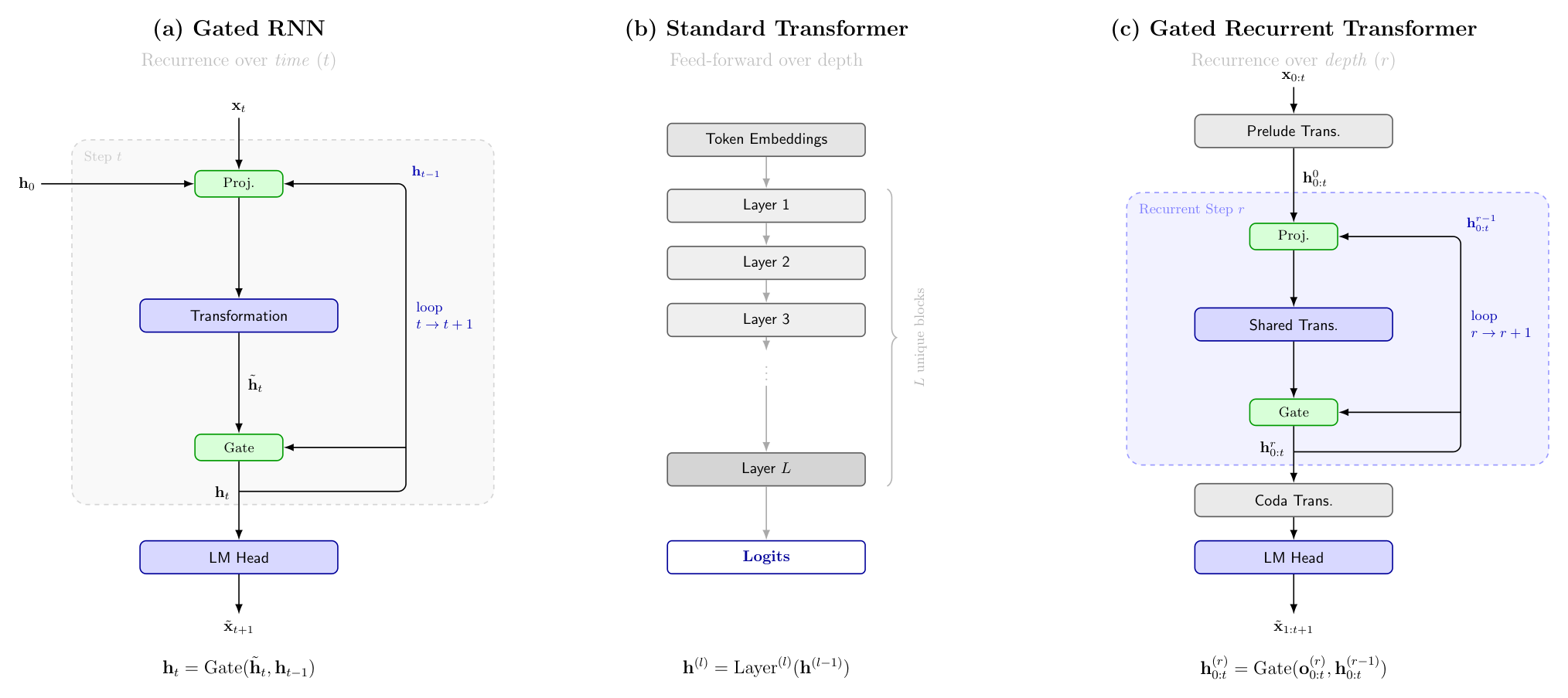
The concept of shared weights across repeated computational steps traces back to the seminal 1986 backpropagation paper of Rumelhart, Hinton, and Williams([14]), who briefly proposed at the end of their paper the synchronous iterative net: a network where each iteration corresponds to a layer with tied weights. ([15]) extended this to temporal sequence modeling via backpropagation through time (BPTT), inspiring recurrent architectures — RNNs ([16]), LSTMs ([17]), and GRUs ([18]) — that apply shared weights along the sequence dimension, processing inputs one timestep at a time. In contrast, this work applies recurrent depth across the full input, iterating a shared-weight transformation along network depth to progressively refine the input representation.

In the era of transformers, one of the earliest papers on recurrent depth was ALBERT ([7]), which proposed a BERT ([19]) model with all transformer layers sharing the same weights. Universal Transformers ([8]) further added a per-token adaptive halting mechanism. However, both methods shared the entire layer stack, forcing every layer to apply an identical transformation regardless of the representational stage of the input. ([9]) relaxed this constraint by assigning distinct roles to prelude, shared core, and coda layers. Similarly, [20] identified early, middle, and late layers of pretrained LLMs as encoding, reasoning, and decoding stages respectively, and proposed recurring only the middle layers while keeping the rest fixed. Our $\textsc{Gated Recurrent Transformer}$ follows this principle of selectively recurring middle layers.

Prior work has shown that parameters in feed-forward network (FFN) layers primarily store factual knowledge ([21]), while computational depth drives reasoning ability ([22]), motivating recurrence to improve reasoning. We organize prior work on recurrent depth transformers along two evaluation regimes. In the iso $\textsc{Params}$ regime — increasing FLOPs by recurring layers while keeping parameter count fixed, trading compute for improved accuracy — ([9, 10, 20]) demonstrate consistent quality gains. In the iso $\textsc{FLOPs}$ regime — reducing parameter count by recurring layers while matching training and inference compute, trading memory for efficiency — ([11]) and ([12]) show that depth reuse can achieve comparable quality at a smaller memory footprint. Our work spans both regimes, with iso $\textsc{FLOPs}$ as our primary contribution and complementary iso $\textsc{Params}$ results reported in Section 4.

A related line of work adapts the amount of computation dynamically rather than fixing it uniformly across tokens or layers. Adaptive Computation Time (ACT) ([23]) halts computation per-position based on learned termination signals, allowing different tokens to consume different amounts of compute. Mixture-of-Depths ([24]) takes a routing approach, dynamically assigning tokens to different subsets of layers rather than processing all tokens through all layers. More recently, Mixture-of-Recursions ([25]) extends this idea to the recurrent setting, routing subsets of tokens to different numbers of recursion steps. While all three methods adapt computation at the token level — through halting, layer routing, or recursion routing — they require dedicated termination signals or routing mechanisms. In contrast, $\textsc{Gated Recurrent Transformer}$ uses a simpler gating mechanism that modulates how much of the shared-block update is absorbed at each recurrence step, without any routing or halting logic.

Weight-tied iteration toward a fixed point is the defining feature of deep equilibrium models ([26]), which solve for the equilibrium directly and differentiate through it with implicit gradients, avoiding the memory cost of storing an unrolled trajectory. $\textsc{Gated Recurrent Transformer}$ shares the weight-tied update but not the equilibrium objective: we unroll a fixed number of discrete steps and backpropagate through them, and depth sampling trains each step to serve as an exit rather than as an approach to a single limit.

Scaling laws ([1, 27]) have established how model size and data jointly determine performance, with Pythia ([28]) providing controlled comparisons across scales. Notably, [1] directly evaluated parameter-sharing transformers and observed that recurrent models perform better at matched parameter count (iso $\textsc{Params}$) but worse at matched compute (iso $\textsc{FLOPs}$). The interplay between depth and width has received dedicated attention: ([29]) theoretically shows that increasing width can compensate for reduced depth in algorithmic reasoning tasks, while ([30]) empirically demonstrates that scaling law prescriptions are sensitive to depth-width ratio. In our $\textsc{Gated Recurrent Transformer}$, we propose a novel recurrent depth architecture that aims to improve the scaling laws of loss versus parameter count and loss versus training FLOPs, demonstrating consistent gains under both iso $\textsc{FLOPs}$ and iso $\textsc{Params}$ regimes as model size and training data scale.

3. Recurrent Depth Reuse for Language Modeling

Section Summary: The section introduces a Gated Recurrent Transformer that reuses a small set of shared blocks multiple times to increase effective model depth without a proportional rise in parameters. The architecture splits processing into an initial prelude stage that builds context, a recurrent core applied repeatedly with a learned projection and elementwise gate to evolve the hidden state, and a final coda stage that produces outputs. This design keeps the total unique parameters fixed while scaling computation through recurrence, drawing on GRU-style gating to maintain stability and preserve information across repeated applications.

3.1 Preliminaries

Let $\mathbf{X} = (x_1, \ldots, x_T)$ be a token sequence of length $T$ drawn from vocabulary $\mathcal{V}$. A standard autoregressive transformer with $L$ blocks defines a chain of residual updates: $\mathbf{h}^{(\ell)} = \mathbf{h}^{(\ell-1)} + \mathrm{Block}\ell(\mathbf{h}^{(\ell-1)})$ for $\ell = 1, \ldots, L$, where $d$ is the embedding dimension and $\mathbf{h}^{(0)} \in \mathbb{R}^{T \times d}$ are initial token embeddings. Each block comprises pre-norm multi-head self-attention and a token-wise MLP. The objective is to minimize the negative log-likelihood, $\mathcal{L} = -\sum_t \log p(x_t \mid x{<t})$. Standard transformers couple depth and parameters rigidly, as every additional layer adds a fresh set of weights. The total unique parameter count scales as $\Theta(L \cdot d^2)$.

3.2 The Prelude–Shared–Coda Architecture

$\textsc{Gated Recurrent Transformer}$ follows ([9]) in partitioning transformer blocks into three sets, denoted by the shorthand $n_{\text{pre}}\texttt{+}n_{\text{rec}}!\times! R\texttt{+}n_{\text{coda}}$. We have observed that this separation of fixed context encoders from a shared recurrent core yields more stable training than uniform weight sharing across all layers.

• Prelude ($n_{\text{pre}}$ blocks): Applied once to produce a stable, context-aware conditioning signal $\mathbf{h}^{(\mathrm{pre})} = \mathrm{Block}{n{\text{pre}}}\circ\cdots\circ\mathrm{Block}_1(\mathbf{h}^{(0)})$.
• Shared core ($n_{\text{rec}}$ blocks): Applied recurrently $R$ times. The first step is initialized with stochastic noise $\epsilon_x$ conditioned on the prelude output. In subsequent steps, the core iteratively processes the previous hidden state $\mathbf{h}^{(r-1)}$ alongside the fixed prelude anchor: $\mathbf{h}^{(R)} = \mathrm{Block}{n{\text{shared}}}\circ\cdots\circ\mathrm{Block}_1[\epsilon_x, , \mathbf{h}^{(\mathrm{pre})}]$. We provide more details on the operation in the subsequent section.
• Coda ($n_{\text{coda}}$ blocks): Receives the final refined state $\mathbf{h}^{(R)}$ and projects to output final hidden state $\mathbf{h}^{(\mathrm{coda})} = \mathrm{Block}{n{\text{coda}}}\circ\cdots\circ\mathrm{Block}_1(\mathbf{h}^{(R)})$ that are then fed into the language model to produce logits.

Total unique parameter count is $\Theta\bigl((n_{\text{pre}} + n_{\text{rec}} + n_{\text{coda}}) \cdot d^2\bigr)$, independent of $R$. A configuration such as 2+5 $\times$ 4+2 visits $2 + 5 \cdot 4 + 2 = 24$ block executions per forward pass while storing weights for only $2 + 5 + 2 = 9$ blocks— $2.6\times$ fewer unique blocks than the 24-layer GPT-2 medium baseline it is isoFLOP-matched to. Figure 2 illustrates this layout.

Per-token forward-pass cost for a $n_{\text{pre}} \texttt{+} n_{\text{rec}}!\times! R \texttt{+} n_{\text{coda}}$ configuration at sequence length $S$ is

$ \text{FLOPs} = \bigl(n_{\text{pre}} + n_{\text{rec}} R + n_{\text{coda}}\bigr)\bigl(24 d^2 + 4 S d\bigr) ;+; R \cdot 10 d^2,\tag{1} $

where $24d^2 + 4Sd$ is the standard per-block cost (attention and MLP projections plus the two attention matmuls) and $10 d^2$ is the per-step overhead of the recurrent projection $W_{\mathrm{proj}}$ and the gate MLP $f_\mathbf{g}$.

3.3 Recurrent Projection and Elementwise Gate

Merely feeding the output of each recurrence as the input to the next recurrence risks forgetting the original input context, suffers from vanishing or exploding gradients across deep recurrences, and taxes the representational capacity of a single shared weight tensor.

Inspired by RNNs ([16]) in general, and GRUs ([18]) in particular, we treat the hidden representation after each recurrence step as a state that evolves across recurrences (as illustrated in Figure 1). Each application of the shared core reads this state, transforms it, and writes an updated state back—analogous to an RNN cell, but operating over depth rather than time. This framing motivates the gating mechanism below: just as GRU gates control how much of its cell state is overwritten at each timestep, $\textsc{Gated Recurrent Transformer}$ 's elementwise gate controls how much of the current depth-state is replaced by the shared block's output.

Hence, we introduce our novel adaptive gating approach that aims to mitigate the 3 aforementioned problems. At each recurrence step $r$, $\textsc{Gated Recurrent Transformer}$ prepares the input to $\mathcal{B}_{\text{shared}}$ by projecting the current state together with the fixed prelude output, then selectively writes the block's output back to the residual stream via a learned elementwise gate. The full update is:

$ \begin{aligned} \tilde{\mathbf{h}}^{(r)} &= W_{\mathrm{proj}}, \bigl[\mathbf{h}^{(r-1)} + \epsilon_x, ; \mathbf{h}^{(\mathrm{pre})}\bigr], \ \mathbf{o}^{(r)} &= \mathcal{B}_{\text{shared}}!\left(\tilde{\mathbf{h}}^{(r)}\right), \ \mathbf{h}^{(r)} &= \mathbf{g}^{(r)} \odot \mathbf{h}^{(r-1)}

• \bigl(1 - \mathbf{g}^{(r)}\bigr) \odot \mathbf{o}^{(r)}, \end{aligned} $

where $[\cdot, \cdot]$ denotes concatenation along the feature axis, $\mathbf{g}^{(r)} \in [0, 1]^{T \times d}$ is a learned elementwise gate (defined in full below , $W_{\mathrm{proj}} \in \mathbb{R}^{d \times 2d}$ is a learned projection, $\epsilon_x \sim \mathcal{N}(0, , \sigma^2 \mathbf{I})$ is injected additive noise, and $\odot$ is elementwise multiplication.

The gate $\mathbf{g}^{(r)} \in [0, 1]^{T \times d}$ is produced by a small feed-forward network conditioned on the normalised current state and the normalised prelude output:

$ \mathbf{g}^{(r)} = \sigma!\left(f_\mathbf{g}!\bigl([\mathrm{LN}(\mathbf{h}^{(r-1)}), ; \mathrm{LN}(\mathbf{h}^{(\mathrm{pre})})]\bigr) / \tau + \epsilon_g \right),\tag{2} $

where $\sigma(\cdot) = 1/(1+e^{-(\cdot)})$ is the sigmoid function, $\mathrm{LN}$ denotes layer normalization ([31]), $\tau$ is a temperature hyperparameter (set to $1.0$ throughout our experiments), $\epsilon_g \sim \mathcal{N}(0, , \sigma_g^2)$ is per-scalar gate noise injected during training, and $f_\mathbf{g}$ is a two-layer MLP with SiLU activation and hidden dimension $d_\text{gate} = d$. The second linear layer of $f_\mathbf{g}$ has its bias initialised to $+4$, placing $\mathbf{g}^{(r)} \approx 0.98$ at the start of training: the copy branch of Eq. dominates, the residual stream passes through the recurrence almost unchanged, and the model learns which elements to overwrite as training proceeds. Positive initialisation of a forget gate is long-standing practice in recurrent networks ([32]), and [33] found a bias of $+1$ or $+2$ enough to bring a vanilla LSTM level with the best variants in their search. We simply apply the same principle over depth rather than time. We swept across ${-2, 0, +2, +4}$ at the full training horizon the spread is $0.019$ nats (Appendix B.6).

By defining $\mathbf{g}^{(r)}{t, i}$ as the $i^{\text{th}}$ element of the gate for token $t$ at recurrence $r$, $\textsc{Gated Recurrent Transformer}$ achieves a highly granular, per-element specialization. When $\mathbf{g}^{(r)}{t, i} \to \mathbf{1}$, the residual stream remains unchanged, whereas $\mathbf{g}^{(r)}_{t, i} \to \mathbf{0}$ allows the block output to fully replace the state. This per-recurrence specialization provides a more memory-efficient alternative to approaches such as Per-Layer Embeddings (PLE) (used in recent models like Gemma3n ([34]) and Gemma-4 ([35])). While PLE requires $L$ unique embedding layers to provide layer-specific context, our approach conditions the gate on $\mathbf{h}^{(\mathrm{pre})}$ to provide a constant view of the original input at every step, while modulating it with $\mathbf{h}^{r-1}$ and stochasticity $\epsilon_g$.

State noise $\epsilon_x$ ( perturbs the recurrent projection input, discouraging the model from learning brittle exact-match patterns across steps. Gate noise $\epsilon_g$ ( prevents the gate from collapsing to a near-constant value during training. Specific noise magnitudes ($\sigma_x$, $\sigma_g$) are reported in Section 4.

3.4 Recurrence Depth Sampling During Training

At each training step, we sample $r \sim \mathrm{Uniform}{1, \ldots, R}$. This serves two purposes: (1) it implicitly trains every exit point, enabling early exit at inference without auxiliary loss terms or the associated gradient interference common in multi-exit models ([36, 37]); and (2) it acts as stochastic depth regularization, improving final validation loss over fixed-depth schedules (as will be shown later in our ablations Section 5.

We summarize the forward pass of $\textsc{Gated Recurrent Transformer}$ in Algorithm 1.

4. Experiments & Results

Section Summary: The experiments trained Gated Recurrent Transformer models from scratch on roughly 9.8 billion tokens using a standard transformer setup, then compared them against dense GPT-2 baselines and other recurrent models under two conditions: equal computation budgets or equal parameter counts. In the equal-computation setting the recurrent model matched or slightly exceeded dense performance while using only 36–37 % as many parameters; when parameter counts were held fixed instead, adding more recurrence steps produced clear gains in validation loss and downstream accuracy. The approach also yielded strong early-exit behavior, letting a single checkpoint deliver usable results at lower depth or higher quality at greater depth without retraining.

Experimental Setup

We build on the nanoGPT codebase ([38]) for our transformer backbone implementation. All models are trained on a diverse dataset of text with sequence length $T = 1024$ tokens and GPT-2 BPE tokenisation (50,257-token vocabulary). We use AdamW ([39]) with $\beta_1 = 0.9$, $\beta_2 = 0.95$, weight decay $0.1$, a 2,000-step linear learning rate warmup, and a cosine learning-rate schedule from a peak of 6 x 10^-4 to 6 x 10^-5.

Gradient norms are clipped at $1.0$. All runs used bfloat16 mixed precision. State noise $\sigma_x = 0.1$ and gate noise $\sigma_g = 0.1$ are used throughout all $\textsc{Gated Recurrent Transformer}$ runs; the gate temperature is fixed at $\tau = 1.0$.

We train for 20,000-steps and use an effective batch size of $\approx$ 491,520 tokens per step (batch size 8, gradient accumulation 60, sequence length 1024), totalling approximately 9.8B tokens per run. Dense baselines (GPT-2 small, medium, and large ([40])) are trained from scratch under the identical setup; no pre-trained weights are used. We train four recurrent competitors from scratch under the same recipe: Mixture-of-Recursions (MoR) ([25]); a variant following [9] that uses the prelude–coda layout with heavy-tail Poisson depth sampling; Relaxed Recursive Transformers (RRT) ([12]), which relaxes weight tying with per-recurrence LoRA adapters; and Ouro ([10]), which supervises every loop iteration.

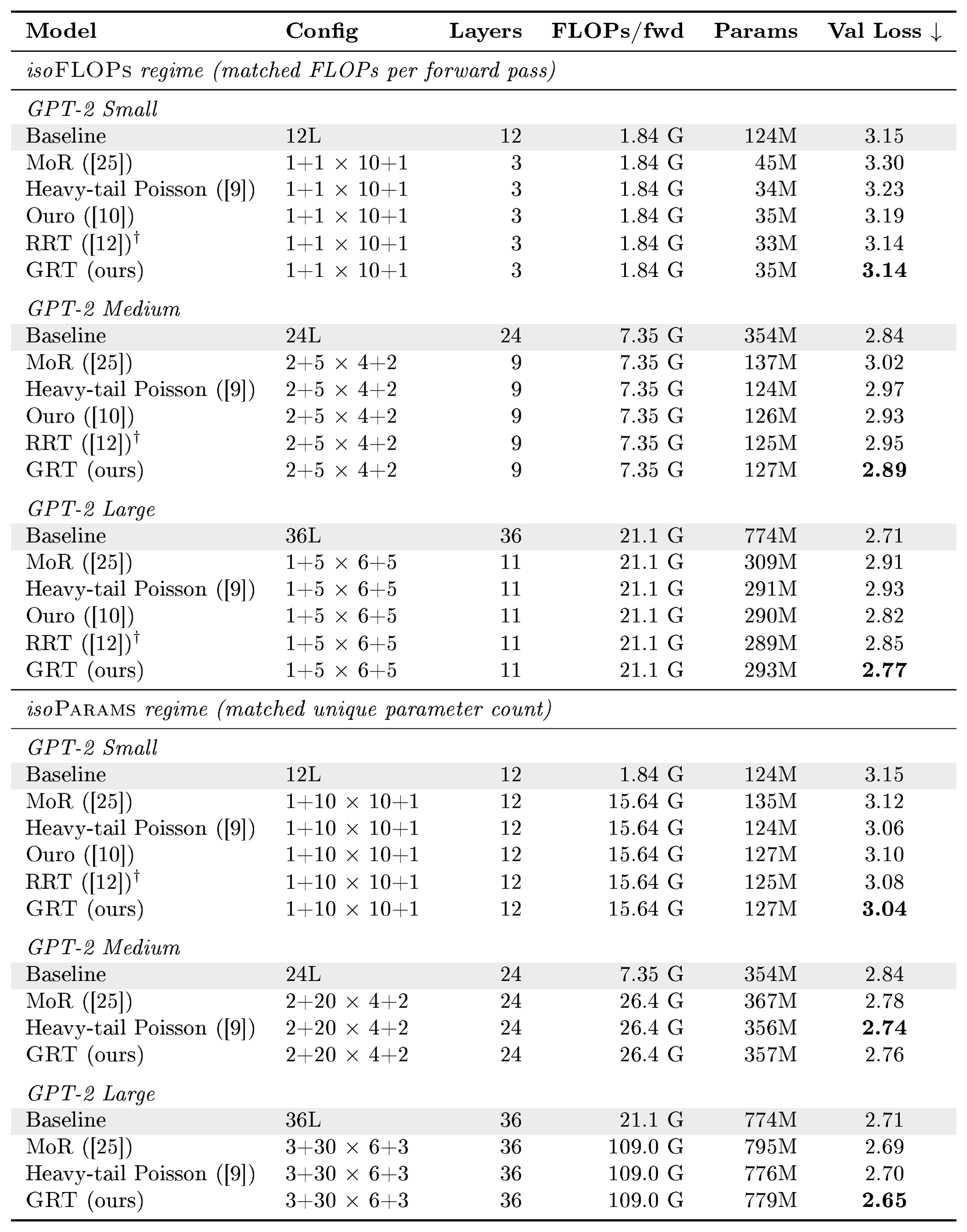
::: {caption="Table 1: Main results (validation loss). Upper: iso FLOPs regime— Gated Recurrent Transformer matches forward-pass FLOPs of the dense baseline with fewer unique parameters. Shaded rows are dense baselines. Lower: iso Params regime—matched unique parameters, higher FLOPs per step. Layers = unique transformer blocks. ↓ lower is better. †RRT adds one LoRA adapter per recurrence, so its weights are not identical across steps."}

:::

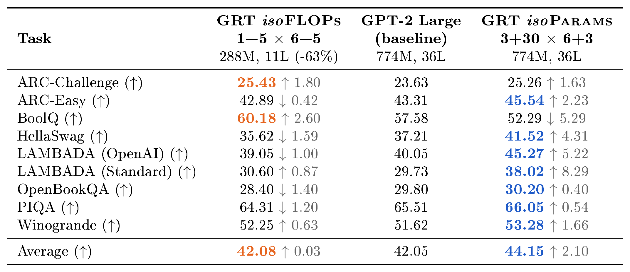
::: {caption="Table 2: Downstream task evaluation (large scale). Zero-shot accuracy on standard benchmarks using lm-eval-harness. ↑ higher is better; deltas relative to GPT-2 Large. Orange: best iso FLOPs result; blue: best iso Params result. The iso Params model outperforms the dense baseline on average by +2.10 points; the iso FLOPs model matches GPT-2 Large at only 37% of its parameter count."}

:::

Main Results

Table 1 summarizes performance across model sizes. In the iso $\textsc{FLOPs}$ regime, $\textsc{Gated Recurrent Transformer}$ achieves competitive quality while storing only 36–37% of the baseline's parameters. At small scale it reaches lower loss than the dense baseline on all three seeds we ran: $3.145 \pm 0.004$ against $3.188 \pm 0.056$, our worst seed at $3.148$ and the baseline's best at $3.154$ (Appendix B.1). At medium and large scale the dense baseline leads at the standard budget, by $0.05$ and $0.06$ nats respectively, and Section 5 shows both gaps closing as the token budget grows.

Against the recurrent baselines the margin widens with scale. RRT is the strongest of the four and reaches parity at small scale, $3.143$ against our $3.141$, a difference well inside the $\pm 0.004$ seed spread; at medium it trails by $0.06$ nats and at large by $0.08$. MoR and heavy-tail Poisson trail by $0.08$ to $0.16$ nats at every scale. We attribute the widening gap to what each method holds fixed. RRT's LoRA deltas are chosen at training time and applied identically to every input, so the diversity they buy is fixed in advance and does not grow with the number of recurrences, whereas the gate conditions on the state it is about to update and keeps successive states separable where uniform sharing collapses them. Ouro is competitive at small scale ($3.19$) but its medium run converged to $2.93$ and its large run converged to $2.82$. Strict weight tying is also what leaves $R^*$ free at inference and produces the early-exit curve of Figure 3a, which a fixed set of adapters cannot produce from a single checkpoint. Appendix B.3 tabulates the design differences alongside training cost.

In the iso $\textsc{Params}$ regime, increasing recurrence $R$ at a fixed parameter budget yields significant gains: a 0.08 nat improvement at Medium scale and 0.06 at Large scale. This demonstrates that for a fixed memory footprint, trading inference FLOPs for recurrent depth is a principled strategy for improving model expressivity.

Table 2 reports accuracy across nine benchmarks at large scale using lm-eval-harness ([41]). The iso $\textsc{FLOPs}$ variant matches the dense model on average (42.08 vs. 42.05), confirming that parameter efficiency translates across evaluation protocols, while the iso $\textsc{Params}$ variant outperforms the dense baseline on eight of nine tasks, consistent with the validation-loss advantage in Table 1.

Early Exit Analysis

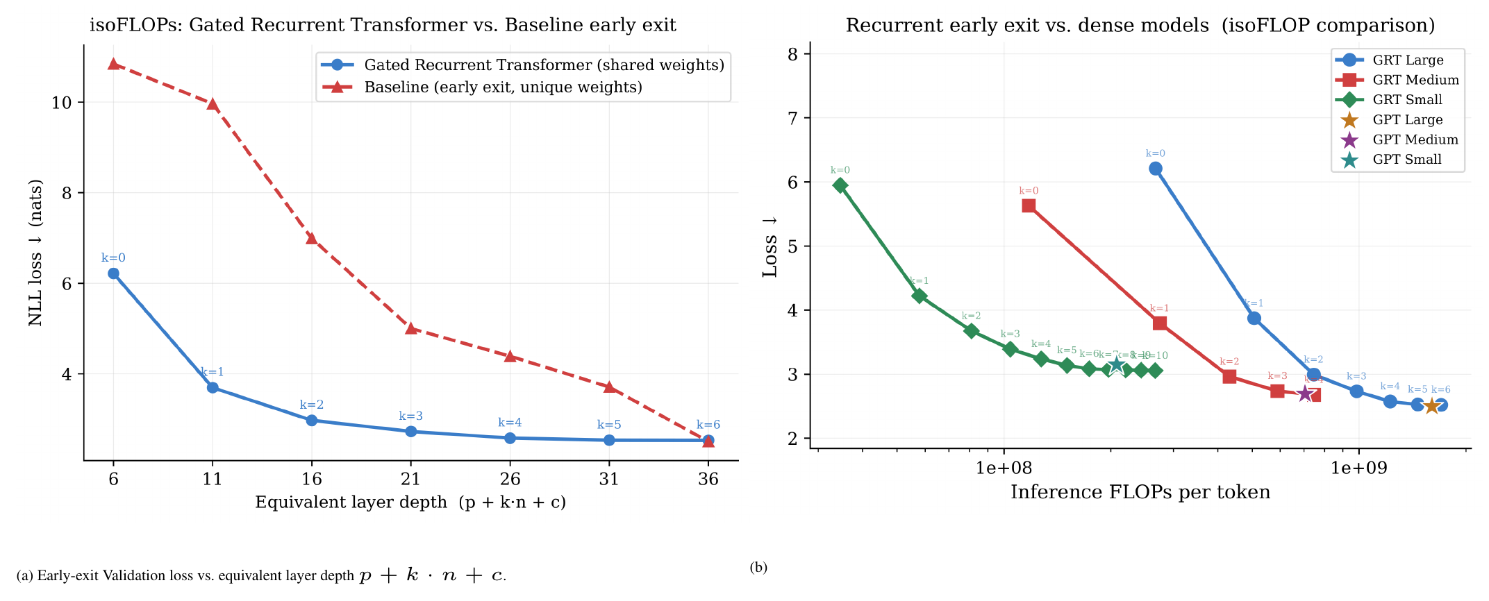
As shown in Figure 3a, $\textsc{Gated Recurrent Transformer}$ exhibits superior early-exit performance as an emergent property: at matched inference FLOPs $\textsc{Gated Recurrent Transformer}$ exiting with fewer recurrences has better loss than a dense model exiting at an earlier layer. Figure 3b extends the analysis across model scales. Because uniform depth sampling (Section 3.4) trains all intermediate recurrent states to predict final losses, the model provides a continuous "compute–quality dial". This allows a single checkpoint to transition from fast, shallow inference to high-quality deep inference without re-training or auxiliary losses.

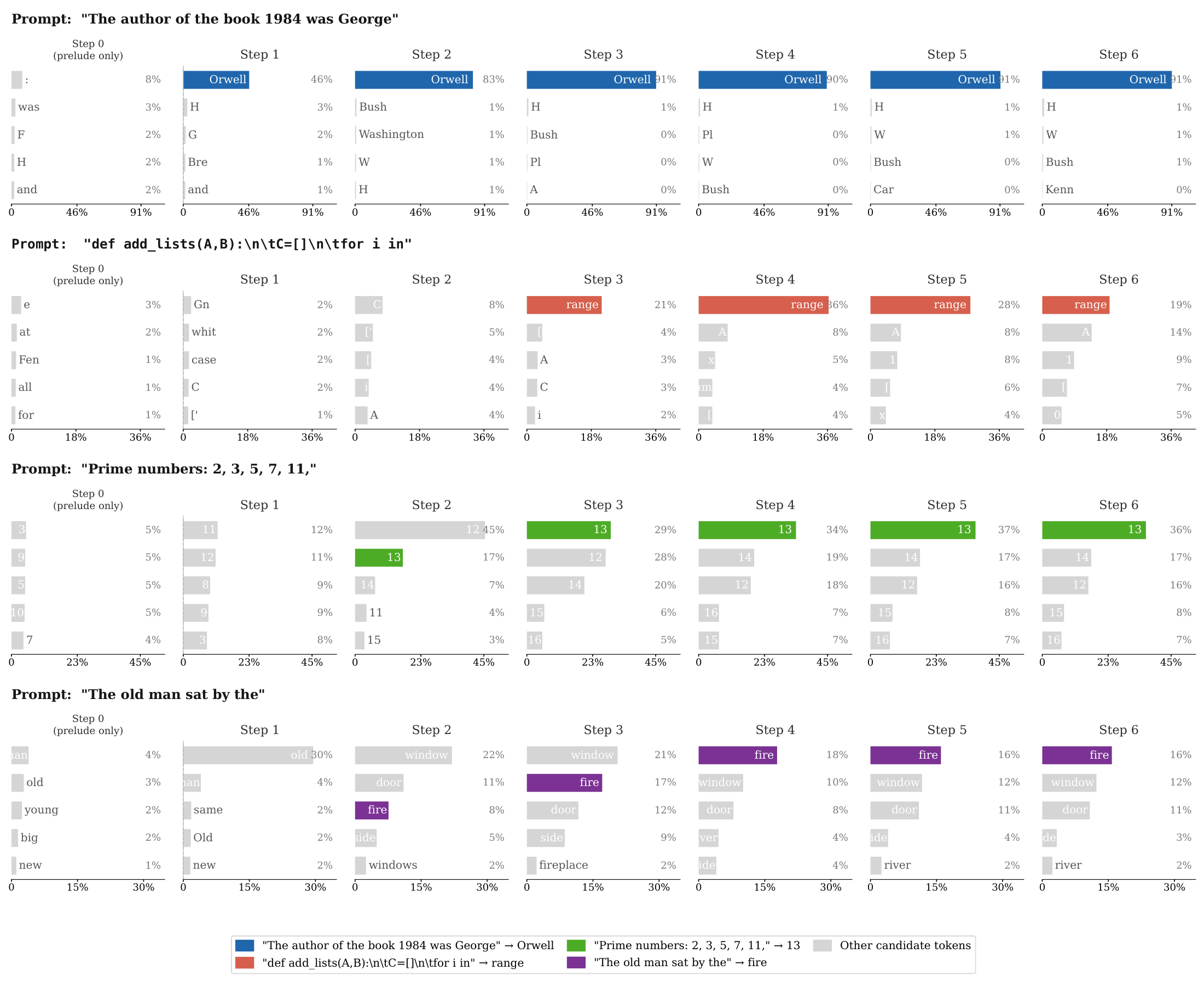
In Figure 4, we provide a qualitative analysis of how next-token predictions evolve across recurrence steps. Our findings reveal that $\textsc{Gated Recurrent Transformer}$ adapts its computational depth to the semantic demands of the prompt: (1) Knowledge-intensive tokens often stabilize early in the recurrence trajectory; (2) Reasoning-based tasks demonstrate progressive error correction and sharpening of the probability mass over deeper iterations; and (3) Open-ended or creative prompts exhibit continuous linguistic refinement, where deeper recurrence enhances local coherence despite the lack of a singular ground truth. This suggests that the model implicitly utilizes the recurrent core to modulate its internal "thinking time" based on task complexity.

KV Cache Sharing

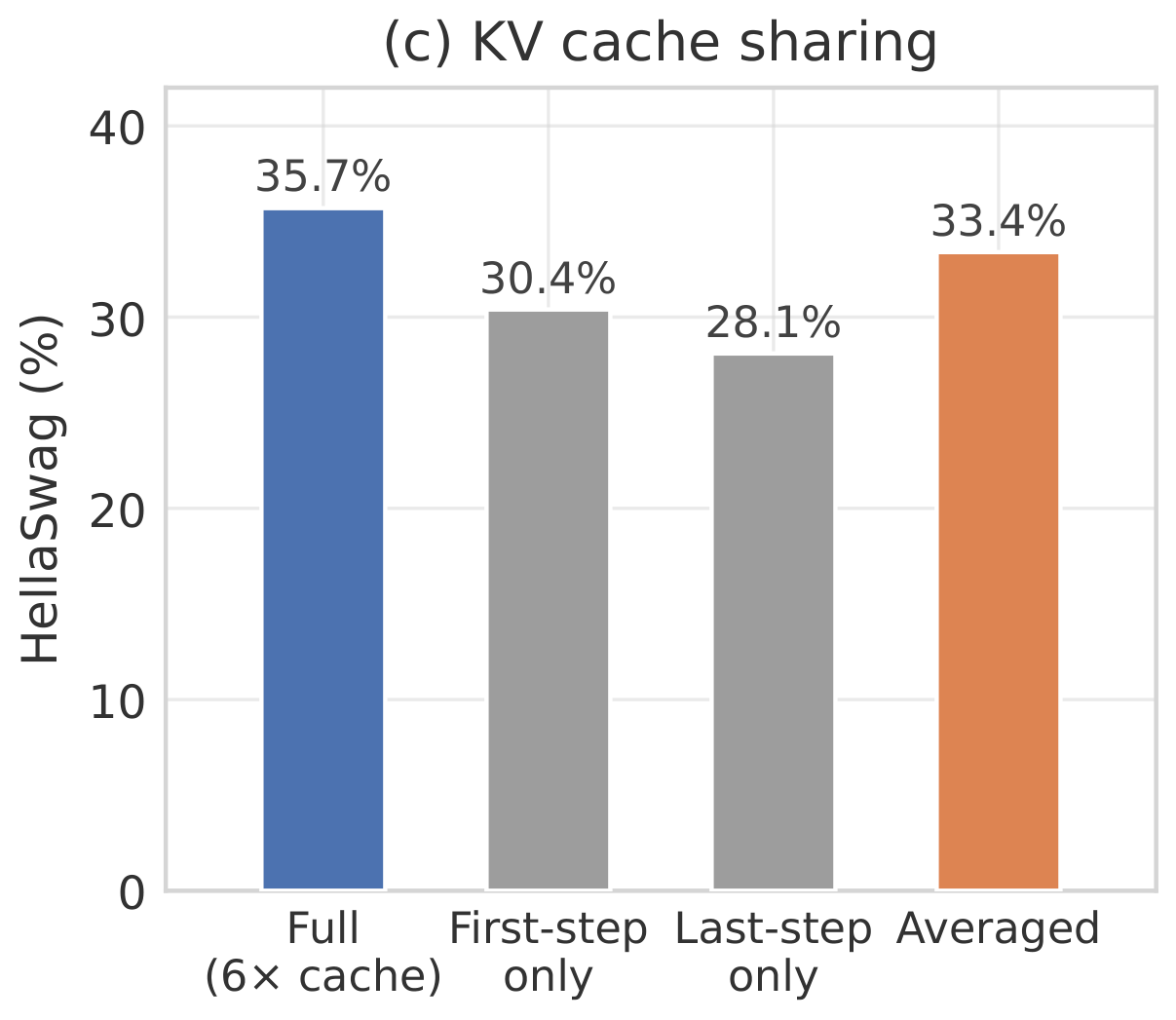
Naively, $\textsc{Gated Recurrent Transformer}$ requires $R$ separate KV caches during decoding—one per recurrence step—multiplying memory by $R$ over a standard transformer. Following ([10]), we evaluate three compressed strategies that each reduce recurrent KV memory over $R$ layers, equivalent to $3.27\times$ reduction across the model: reusing only the last step's cache, only the first step's, or an averaged K/V across steps. As shown in Figure 7, we observe that averaged leads to best accuracy, while last leads to the worst accuracy.

Wall-Clock Latency and Decoding Memory

$\textsc{Gated Recurrent Transformer}$ executes the same number of block applications as the dense model it is iso $\textsc{FLOPs}$-matched to, distributed over fewer unique weight tensors. Table 3 reports measured generation latency and peak GPU memory on identical hardware (batch size 4, prompt length 1024, 128 generated tokens). Under torch.compile, $\textsc{Gated Recurrent Transformer}$-Large costs $+10%$ generation latency for $62%$ fewer parameters and $59%$ less peak memory; at medium scale the overhead is $+11%$. In eager mode both overheads are $+23%$, so roughly half the gap is kernel-launch overhead from the additional elementwise operations rather than arithmetic.

: Table 3: Generation latency and peak memory (iso $\textsc{FLOPs}$ configurations). Batch size 4, prompt length 1024, 128 generated tokens, same hardware. Both arms are measured under torch.compile and in eager mode.

Model	Config	Params	Eager (ms/tok)	Compiled (ms/tok)	Peak mem.
GPT-2 Medium	24L	354M	2.95	2.54	747 MB
GRT Medium	2+5 × 4+2	127M	3.62	2.81	402 MB
GPT-2 Large	36L	774M	4.33	3.33	1570 MB
GRT Large	1+5 × 6+5	293M	5.33	3.67	639 MB

The $R\times$-expanded KV cache is a real cost, and whether it erodes the parameter saving depends on batch size. Table 4 reports end-to-end decoding memory (weights $+$ KV, bf16, $T=1024$) for the medium iso $\textsc{FLOPs}$ checkpoint. At $B{=}1$ decoding is weight-dominated and the parameter reduction lands at $0.55\times$ dense memory even with the naive $R\times$ cache; at $B{=}32$ the cache dominates and the naive strategy recovers only $0.91\times$. Averaging K/V across recurrence steps brings this to $0.39\times$ while improving HellaSwag accuracy over the full cache ($33.90$ vs. $33.65$), which suggests the averaging acts as a mild regulariser at this scale.

\begin{tabular}{lccc}
  \toprule
  \textbf{Configuration} & \textbf{HellaSwag} & Mem. @ $B{=}1$ & Mem. @ $B{=}32$ \\
  \midrule
  GPT-2 Medium (24L, 354M) & \textbf{34.45} & 0.75 GiB (1.00 $\times$) & 3.66 GiB (1.00 $\times$) \\
  \textsc{GRT} \textit{iso\textsc{FLOPs}}, full $R\times$ KV & 33.65 & 0.41 GiB (0.55 $\times$) & 3.32 GiB (0.91 $\times$) \\
  \textsc{GRT} \textit{iso\textsc{FLOPs}}, averaged KV & 33.90 & 0.35 GiB (0.47 $\times$) & 1.44 GiB (0.39 $\times$) \\
  \bottomrule
  \end{tabular}

Mechanistic Analysis Summary

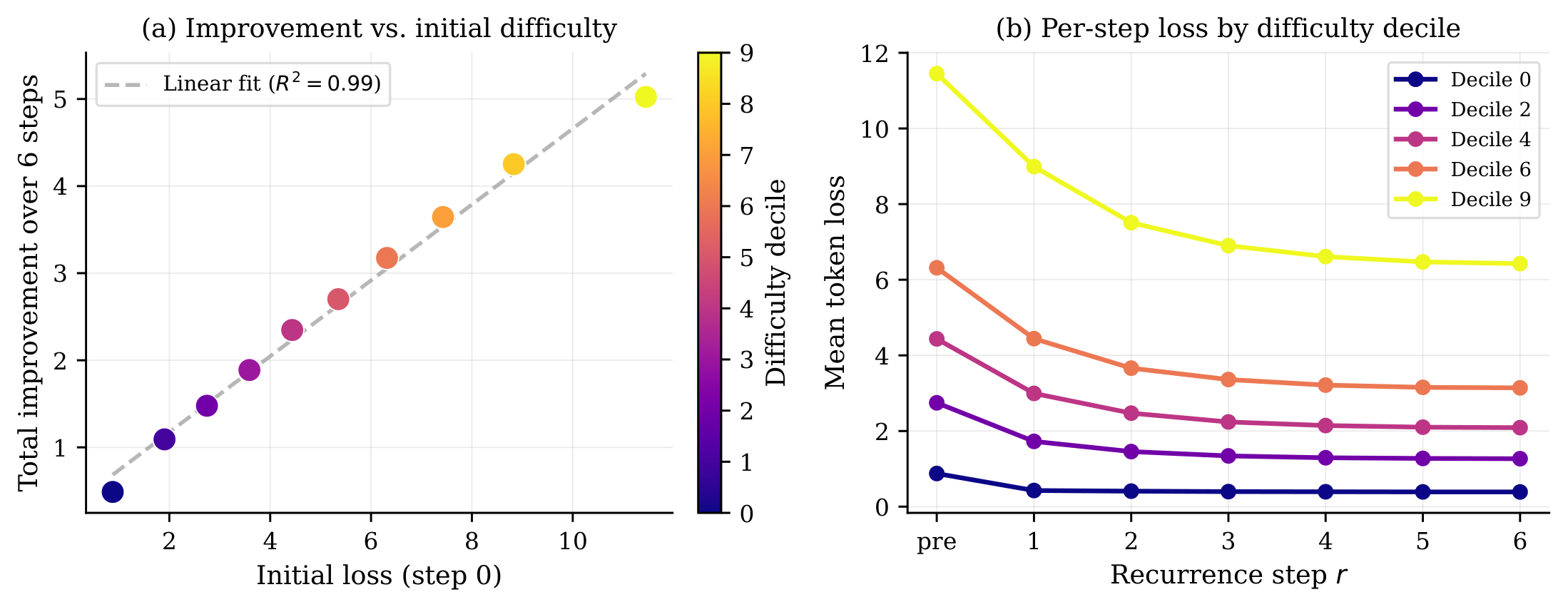
Detailed mechanistic analysis of the large 1+5 $\times$ 6+5 checkpoint is provided in Appendix E; we summarise the key findings here. We observe in Figure 10 that gate, $g^{(r)}$, behavior evolves across recurrence steps: early recurrences ($r \leq 2$) are write-heavy (gate values near $0$, block output dominates), while later steps transition to copy-heavy behavior (gate near $1$, residual stream preserved), consistent with a coarse-to-fine computation strategy. Centered Kernel Alignment ([42]) analysis in Figure 12 confirms that representations across recurrence steps are more similar to one another than representations across layers in a standard transformer of matched depth, suggesting the shared block learns a broadly applicable transformation rather than depth-specialized ones. In Figure 13, we observe that tokens that are more difficult for the model accumulate $10\times$ more improvement across recurrence steps, demonstrating implicit compute routing toward harder inputs without any explicit difficulty signal.

5. Ablations

Section Summary: The section examines how each part of the Gated Recurrent Transformer contributes to performance and how the model scales with different amounts of training data. Component tests on a small model show that recurrence initially increases loss by mixing processing steps, but adding boundaries, noise, re-injection, and especially an elementwise gate progressively improves results, with the full design eventually beating a standard dense baseline. Data-scaling experiments reveal that the recurrent approach maintains an advantage across data sizes at smaller scales, while at larger scales it starts behind but catches up as the data budget grows.

We study two complementary aspects of $\textsc{Gated Recurrent Transformer}$: the contribution of each architectural component (Section 5) and the model's behaviour as the training data budget varies (Section 5). All ablations use validation loss as the primary metric.

Component Ablation

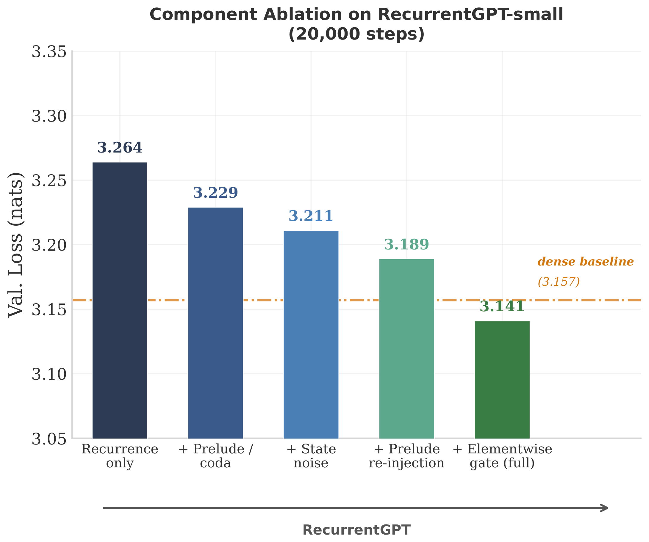
Figure 5 traces a sequential ablation on the small model at the full 20,000-step budget. Recurrence alone raises validation loss by 0.107 nats: without a mechanism to differentiate steps, the shared block conflates early and late processing into a single weight tensor. Adding prelude and coda boundaries (row 3) recovers 0.035 nats; state noise (row 4) contributes 0.018 more, which also isolates the value of injecting noise at every step rather than only at initialisation. Prelude re-injection into each recurrence (row 5) cuts loss by a further 0.022 nats. The elementwise gate (row 6) is the single largest contributor at $-$ 0.048 nats.

Data Efficiency

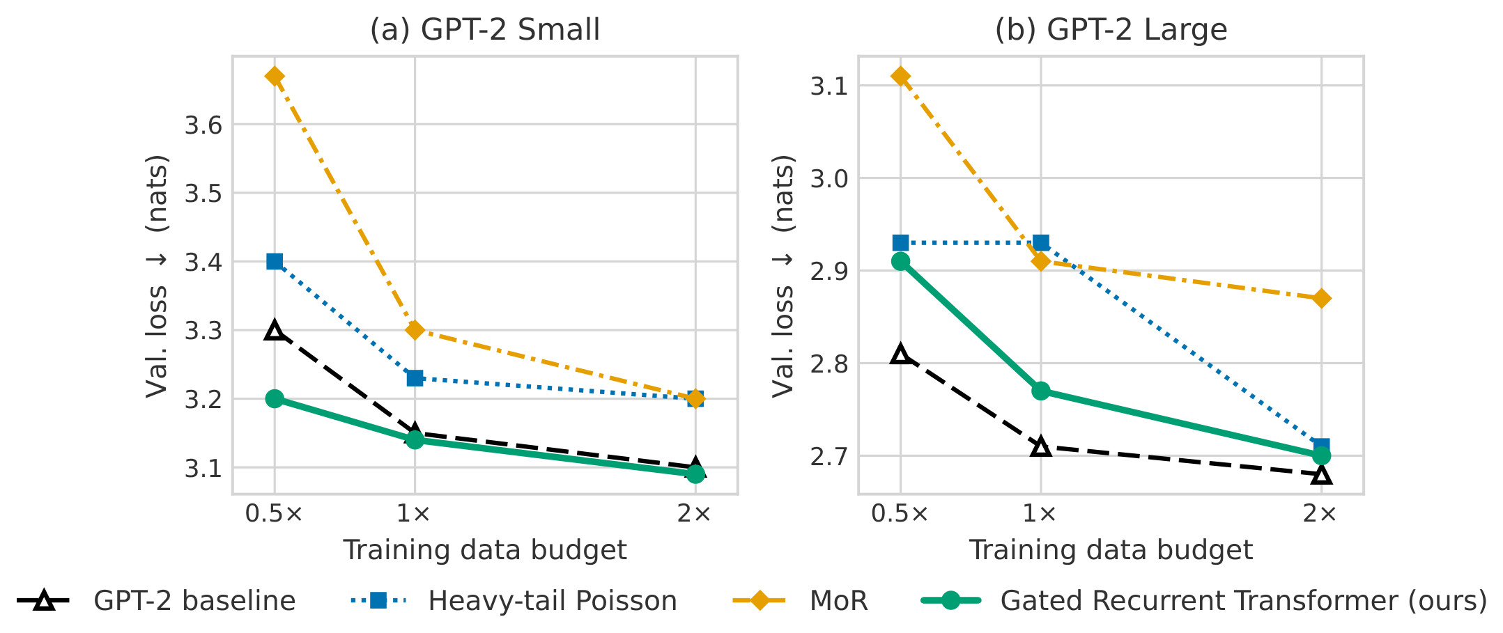
As illustrated in Figure 6, we analyze the performance of recurrent depth across varying training data budgets. At smaller model scales, $\textsc{Gated Recurrent Transformer}$ consistently maintains a superior Pareto frontier compared to the dense baseline across all observed data volumes. At larger scales, a more complex "crossover" dynamic emerges: while the dense model shows an initial lead under low-data regimes, the gap narrows significantly as the token budget increases. For the Large-scale configuration, the trajectories converge at higher data budgets, suggesting that recurrent sharing is particularly effective at saturating parameter capacity when provided with sufficient data.

6. Conclusion

Section Summary: The Gated Recurrent Transformer introduces a learned gating mechanism that conditions each element on the current hidden state, a fixed initial output, and added noise, allowing the model to increase its effective depth without adding many new parameters. In experiments with fixed computation budgets it uses roughly one-third the parameters of a standard dense model yet outperforms prior recurrent approaches on both validation loss and downstream tasks, while fixed-parameter tests show further gains from greater recurrence depth. The approach still relies on a preset recurrence depth at inference time, may need retuning for other model families, and leaves open questions about how much parameter sharing works best at different scales.

$\textsc{Gated Recurrent Transformer}$ demonstrates that a learned per-element gate conditioning on the current hidden state, the fixed prelude output, and injected stochastic noise is a principled strategy for decoupling model depth from parameter count. Under an iso $\textsc{FLOPs}$ constraint, $\textsc{Gated Recurrent Transformer}$ stores only $36$ – $37%$ of the dense baseline's unique parameters while beating both MoR ([25]) and heavy-tail Poisson sampling at every scale; under an iso $\textsc{Params}$ constraint, deeper recurrence yields consistent validation-loss gains (Table 1) and downstream improvements of up to $+8.29$ points (Table 2). Three limitations bound the current work: the recurrence depth $R$ is fixed at inference with no per-token halting ([23]); the gate bias and noise magnitudes may require re-tuning beyond the GPT-2 family; and the scale-dependent optimal sharing fraction warrants systematic study. Future directions include dynamic per-token halting and knowledge distillation from a dense language model into a recurrent student.

Appendix

Section Summary: The appendix presents the forward-pass algorithm for the Gated Recurrent Transformer, showing how token embeddings are processed through fixed prelude and coda blocks around a variable number of shared recurrent steps that incorporate Gaussian noise, a learned per-element gate, and a frozen pre-recurrence anchor. It supplies the full training hyperparameters for the reported GPT-2 and GRT model sizes and includes ablation tables that quantify run-to-run variance across seeds, the incremental effect of each architectural component at short training horizons, and the design distinctions between this approach and other recurrent-depth methods.

A. Implementation Details

def grt_forward(x, model, R, r_min=1):      # R = max recurrence depth
    h = token_embed(x) + pos_embed(x)             # [S, d]
    for block in model.prelude_blocks:
        h = h + block(h)
    h_pre = h                                   # h^(0) = h^(pre): frozen anchor
    r = R if not training else uniform_sample(r_min, R)  # depth sampling
    for step in range(r):                # r in {0,...,R-1}
        eps = sample_gaussian(0, sigma**2)  
        h_tilde = W_proj( cat([h + eps, h_pre]) ) # concat -> project to d
        o = B_shared(h_tilde)                     # same weights every step
        eps_g = sample_gaussian(0, sigma_g**2)
        g = sigmoid(f_gate(LN(h), LN(h_pre))/tau + eps_g) # gate in [0,1]^{Sxd}
        h = g * h + (1 - g) * o                  # gated residual update
    for block in model.coda_blocks:
        h = h + block(h)
    return lm_head(h)                        # [S, |V|]

A.1 Hyperparameter Table 5 lists the full training configuration for every run reported in the main paper.

: Table 5: Training configurations. $p$: prelude blocks; $b$: shared blocks; $R$: recurrence steps; $c$: coda blocks; $d$: embedding dimension; $h$: attention heads. Batch tokens = batch_size × gradient_accumulation × sequence_length × num_GPUs. All runs use AdamW ($\beta_1=0.9$, $\beta_2=0.95$), weight decay 0.1, gradient clip 1.0, bfloat16 mixed precision, cosine LR schedule.

Run	$p$	$b$	$R$	$c$	$d$	$h$	Batch tokens	Peak LR	Steps	Hardware
GPT-2 Small (baseline)	---	---	---	---	768	12	491, 520	6 × 10⁻⁴	20k	2 × H200
GRT Small (isoFLOP)	1	1	10	1	768	12	491, 520	6 × 10⁻⁴	20k	2 × H200
GPT-2 Medium (baseline)	---	---	---	---	1024	16	491, 520	6 × 10⁻⁴	20k	2 × H200
GRT Medium (isoFLOP)	2	5	4	2	1024	16	491, 520	6 × 10⁻⁴	20k	2 × H200
GRT Medium (isoParam)	2	20	4	2	1024	16	491, 520	6 × 10⁻⁴	20k	2 × H200
GPT-2 Large (baseline)	---	---	---	---	1280	20	491, 520	6 × 10⁻⁴	20k	2 × H200
GRT Large (isoFLOP)	1	5	6	5	1280	20	491, 520	6 × 10⁻⁴	20k	2 × H200
GRT Large (isoParam)	3	30	6	3	1280	20	491, 520	6 × 10⁻⁴	20k	2 × H200

All recurrent runs use gate bias initialisation $+4$ ($\mathbf{g} \approx 0.98$ at init), state noise $\sigma_x = 0.1$, gate noise $\sigma_g = 0.1$, and gate temperature $\tau = 1.0$. During training, recurrence depth is sampled uniformly from ${1, \ldots, R}$ at each training step.

B. Additional Ablations

B.1 Run-to-Run Variance Across Seeds

Table 6 reports three independent training runs (seeds 1337, 42, 123) of the small iso $\textsc{FLOPs}$ configuration and of its dense counterpart, all at the full 20,000-step budget. $\textsc{Gated Recurrent Transformer}$ averages $3.145 \pm 0.004$ against $3.188 \pm 0.056$ for the dense baseline. $\textsc{Gated Recurrent Transformer}$ 's worst seed ($3.148$) still falls below the dense baseline's best ($3.154$). Seed 1337 is the run reported throughout the main paper.

\begin{tabular}{lcccc}
  \toprule
  \textbf{Model} & \textbf{Seed 1337} & \textbf{Seed 42} & \textbf{Seed 123}
   {} & Mean $\pm$ std \\
  \midrule
  Dense baseline (12L) & 3.154 & 3.156 & 3.253 & $3.188 \pm 0.056$ \\
  \textsc{GRT} (\texttt{1+1 $\times$ 10+1}) & \textbf{3.141} & \textbf{3.146}
   {} & \textbf{3.148} & $\mathbf{3.145 \pm 0.004}$ \\
  \bottomrule
  \end{tabular}

B.2 Component Ablation at Short Horizon

Table 7 reports the sequential ablation of Section 5 run on the medium configuration at 2,000 steps. At this horizon the ordering of the last two rows is inverted relative to the full 20,000-step run: prelude re-injection contributes $-0.198$ nats against the gate's $-0.115$. We report both because the comparison is itself informative — the structural components land early, whereas the gate is a learned mechanism whose contribution accrues over training.

\begin{tabular}{clcc}
  \toprule
   {} & \textbf{Configuration} & \textbf{Val. loss} & $\boldsymbol{\Delta}$ \\
  \midrule
  1 & Dense baseline (non-recurrent) & 3.621 & --- \\
  \midrule
  2 & Recurrence & 4.163 & +0.542 \\
  3 & \quad + Prelude / coda ($2{+}\_+2$) & 4.118 & -0.045 \\
  4 & \quad + State noise ($\sigma_x{=}0.1$) & 4.099 & -0.019 \\
  5 & \quad + Prelude re-injection & 3.901 & $-$ \textbf{0.198} \\
  6 & \quad + Elementwise gate (full \textsc{Gated Recurrent Transformer}) & \textbf{3.786} & -0.115 \\
  \bottomrule
  \end{tabular}

B.3 Design Comparison of Recurrent-Depth Methods

Table 8 sets the small-scale results of Table 1 beside the design choices that produce them. MoR and Ouro gate the update, but Ouro supervises every iteration and MoR needs a router; heavy-tail Poisson shares strictly and updates unconditionally; RRT is input-independent and depth-fixed. $\textsc{Gated Recurrent Transformer}$ is the only column combining full sharing, an input-dependent update, and variable inference depth.

\begin{tabular}{lcccccc}
\toprule
\textbf{Property} & \textbf{Dense} & \textbf{MoR} & \textbf{Poisson} &
\textbf{RRT} & \textbf{Ouro} & \textbf{\textsc{GRT}} \\
  {} & & \scriptsize([25]) & \scriptsize([9])
  {} & \scriptsize([12]) & \scriptsize([10]) & \textbf{(ours)} \\
\midrule
Full weight sharing & n/a & Yes & Yes & No (LoRA) & Yes & \textbf{Yes} \\
Variable inference depth & No & Yes & Yes & No & Yes & \textbf{Yes} \\
Input-dependent gating & No & Yes & No & No & Yes & \textbf{Yes} \\
Per-step noise injection & No & No & Init only & No & No & \textbf{Yes} \\
Per-iteration loss & No & No & No & No & Yes & No \\
Emergent early exit & No & Yes & Yes & No & Yes & \textbf{Yes} \\
\midrule
Training time (small) & 3h18m & 12h19m & 4h16m & 6h42m & 8h20m & 6h18m \\
Small val. loss $\downarrow$ & 3.15 & 3.30 & 3.23 & 3.14 & 3.19 & \textbf{3.14} \\
\bottomrule
\end{tabular}

B.4 Gate Temperature Sensitivity

The gate temperature $\tau$ ( controls the sharpness of the sigmoid. We sweep $\tau \in {0.5, 1.0, 2.0}$ on the medium configuration at 5,000 steps. Validation loss is 3.62, 3.60, and 3.63 respectively, indicating that the optimal gate temperature is $\tau=1.0$.

B.5 Noise Magnitude Sensitivity

We ablate state noise $\sigma_x \in {0.0, 0.05, 0.1, 0.2}$ on the medium configuration at 5,000 steps. Removing noise entirely ($\sigma_x=0.0$) increases validation loss by 0.031 nats relative to $\sigma_x=0.1$; larger noise ($\sigma_x=0.2$) degrades by 0.018 nats. The optimal range is $\sigma_x \in [0.05, 0.1]$; we use 0.1 throughout.

B.6 Gate Bias and State Noise at Full Training Horizon

The sweeps above are at 5,000 steps. We repeated both at the full 20,000-step budget on the small configuration to check that the response surface does not sharpen at convergence. It does not. Moving the gate bias from the default $+4$ down to $0$ costs $0.019$ nats, and $-2$ recovers to $3.151$; the surface is shallow and non-monotonic rather than peaked, and no setting produced a loss spike or divergence. State noise behaves the same way: removing it costs $0.018$ nats and doubling it costs $0.019$, a symmetric optimum rather than a value that has to be hit precisely. This is weaker evidence than a cross-architecture study, but it does suggest the mechanism does not depend on the exact bias value.

\begin{tabular}{lc}
  \toprule
  \textbf{Gate bias} & Val. loss $\downarrow$ \\
  \midrule
  $+4$ (default) & \textbf{3.141} \\
  $+2$ & 3.152 \\
  $0$ & 3.160 \\
  $-2$ & 3.151 \\
  \bottomrule
  \end{tabular}

\begin{tabular}{lcc}
  \toprule
  $\sigma_x$ & Val. loss $\downarrow$ & $\boldsymbol{\Delta}$ \\
  \midrule
  $0$ & 3.229 & +0.018 \\
  $0.1$ (default) & \textbf{3.211} & --- \\
  $0.2$ & 3.230 & +0.019 \\
  \bottomrule
  \end{tabular}

C. Additional Qualitative Results

C.1 Per-Token Gate Activations Across Recurrence Steps

Figure 8 shows $\bar{g}^{(r)}_t = \mathrm{mean}d(g^{(r)}{t, :})$ — the elementwise gate averaged over the model dimension — for each token position $t$ and recurrence step $r$, on four example prompts. Brighter (yellow-green) cells indicate write-heavy positions where the gate is open ($\bar{g} \approx 0.70$ – $0.82$) and the shared block's proposal is substantially absorbed; darker (purple) cells indicate copy-heavy positions ($\bar{g} \approx 0.95$ – $1.00$) where the hidden state passes through largely unchanged.

Three consistent observations emerge across all four prompts. First, the per-step mean gate rises monotonically from step 2 onward: means fall from $\sim$ 0.87–0.89 at step 1 to a minimum around step 2 (write-heavy phase), then recover steadily toward $\sim$ 0.88–0.91 at step 6 (copy-heavy phase). Second, write-heavy positions are structurally consistent across steps: the same columns that light up at step 1 tend to be the same at step 6, indicating that token identity — not recurrence depth — drives the gate primary signal, with the gate progressively dimming those writes over steps rather than shifting which tokens are written. Third, content words and syntactically load-bearing tokens receive lower gate values than function words: in "The old man sat by the", man and sat are visibly brighter than the and by; in the code prompt, the operator and identifier tokens show write-heavy behaviour while keywords like def and for are copy-heavy. This implicit routing — without any explicit per-token mechanism — arises purely from the gate conditioning on both the evolving hidden state $x^{(r)}$ and the fixed prelude anchor $h$.

D. Broader Impact

Parameter-efficient language models have direct environmental and accessibility benefits: a $\textsc{Gated Recurrent Transformer}$ checkpoint at 37% of a baseline's parameter count requires proportionally less GPU memory at serving time, enabling deployment on hardware that cannot accommodate the full dense model and reducing energy consumption per inference step. Recurrent depth also provides a natural compute-quality tradeoff at inference time—the early-exit capability of Section 4 allows a single trained model to serve requests at multiple quality-FLOPs operating points without retraining.

The risks associated with $\textsc{Gated Recurrent Transformer}$ are not specific to its architecture: as a capable language model trained on web text, it inherits the standard dual-use risks of any such system, including the potential to generate misinformation or harmful content. These risks are addressed by standard deployment safeguards (content filtering, output monitoring, and responsible release practices) that apply equally to all current language models; the recurrent architecture does not introduce qualitatively new threat vectors.

E. Recurrence Dynamics Analysis

Beyond aggregate validation loss, we probe what the shared block computes at each recurrence step $r \in {1, \ldots, 6}$ using the large 1+5 $\times$ 6+5 checkpoint. Diagnostics are run on a validation split with inference noise disabled. We report ten interlocking findings—grouped first into behavioural diagnostics (Appendix E.1–Appendix E.6) and then into mechanistic analyses of weights and attribution (Appendix E.7–Appendix E.10)—before drawing them together in Appendix E.11.

E.1 Rapid Convergence of Loss Across Recurrence Steps

Figure 9(a) traces the per-step validation loss as the shared block is applied iteratively. The prelude output alone yields a loss of $5.29$; after a single application of the shared core the loss drops to $3.77$ —a reduction of $1.52$ nats (natural-log-scale bits; 1 nat $= \log_2 e \approx 1.44$ bits) in one step. By step 2 the loss reaches $3.14$, and the remaining four steps account for only an additional $0.46$ nats, converging to the final value of $2.68$. Stated differently, the first two recurrence steps account for roughly 77% of the total loss reduction from the prelude representation to the final output.

This front-loaded profile is confirmed by the KL-divergence trajectory in Figure 9(b), which measures residual uncertainty relative to the final-step output distribution. The KL falls from $2.61$ at the prelude to $0.46$ by step 2 and reaches $0.014$ at step 5, indicating that the output distribution is essentially committed after the fourth step. As a lower bound on the gate's utility, forcing the gate to zero throughout (the "no-recurrence" ablation) yields a catastrophic loss of $12.03$, confirming that the iterative refinements are not redundant. The complementary ablation—forcing the gate to one throughout, so that every block proposal is discarded and the hidden state is never updated—yields a loss of $5.26$, equivalent to the prelude-only output ($5.26$ at step $r=0$). This confirms that recurrence with a fully open gate is vacuous: without selective writing, six recurrence steps reduce to a single prelude pass. Together, Gate=0 ($12.03$) and Gate=1 ($5.26$) bracket the trained model ($2.68$): the learned gate neither skips recurrence nor blindly overwrites state, but acquires a fine-grained elementwise balance between retention and update.

We also evaluate extending the recurrence depth at inference time beyond the $R=6$ steps seen during training. Applying the trained shared block for $R \in {8, 10, 12}$ steps marginally degrades performance ($2.69$, $2.72$, $2.74$ respectively), suggesting the model has converged representationally by step 6 and that additional steps introduce noise rather than refinement.

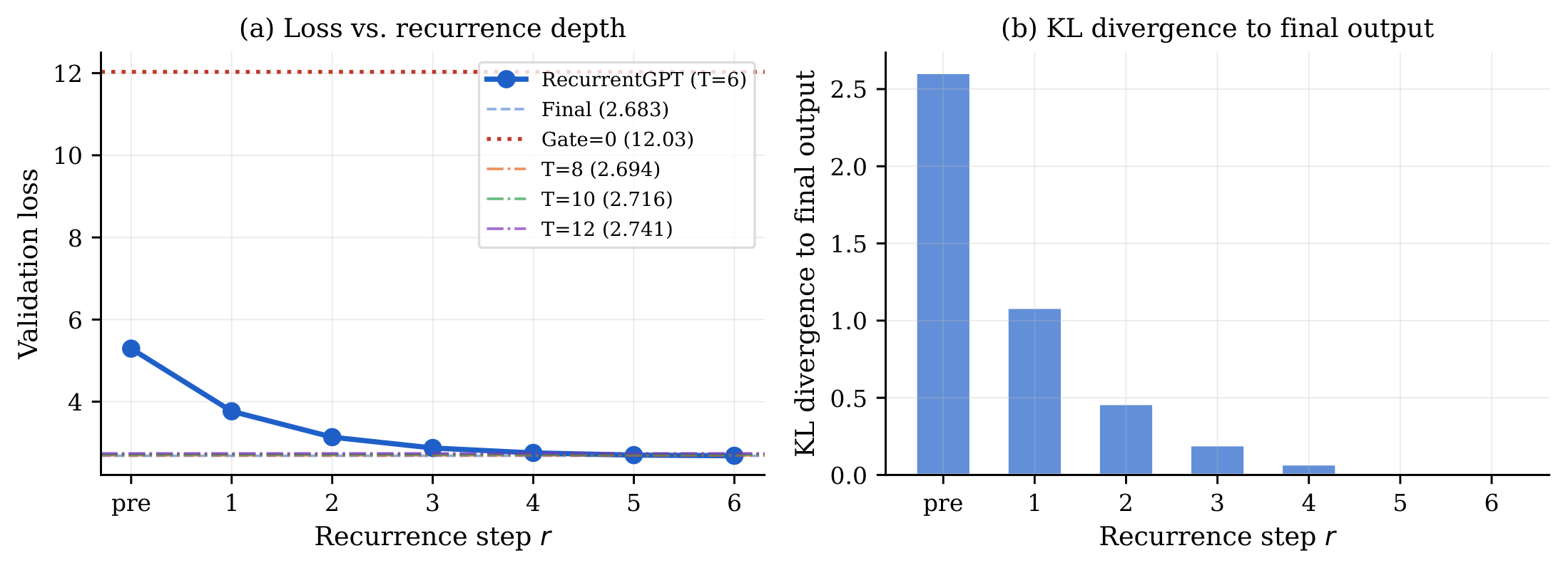
77% of the loss reduction from prelude to final output occurs within the first
  two recurrence steps; the remaining four steps provide targeted corrections.

  The model's output distribution is essentially committed by step 4.

E.2 Gate Behaviour: Write-Heavy Early, Copy-Heavy Late

The elementwise gate $\mathbf{g}^{(r)} \in [0, 1]^{S \times d}$ controls how much of the shared block's proposal is written into the residual stream at each step. Figure 10(a) plots the per-step mean and standard deviation. The gate is most open—and most variable—in the middle steps (steps 2–3, mean $\approx 0.82$, std $\approx 0.18$), corresponding to the highest information-writing regime, and tightens progressively toward step 6 (mean $0.87$, std $0.12$).

Figure 10(b) quantifies this transition via the fraction of dimensions where the gate is near-saturated. Copy-saturated dimensions ($g > 0.95$) grow monotonically from 19.7% at step 1 to 28.8% at step 6, while write-saturated dimensions ($g < 0.05$) remain negligibly rare (

lt;10^{-4}$) throughout. This asymmetry—abundant copying, scarce full-overwriting—indicates the model prefers selective blending over clean state replacement.

The effective gate openness (Figure 10(c)), measured as the ratio

$ \rho^{(r)} = \frac{| \mathbf{h}^{(r)} - \mathbf{h}^{(r-1)}|_2}{|\mathbf{o}^{(r)} - \mathbf{h}^{(r-1)}|_2} = \frac{|(1 - \mathbf{g}^{(r)}) \odot (\mathbf{o}^{(r)} - \mathbf{h}^{(r-1)})|_2}{|\mathbf{o}^{(r)} - \mathbf{h}^{(r-1)}|_2},\tag{3} $

where the numerator is the norm of the applied update (actual change to the hidden state) and the denominator is the norm of the proposal (the full update the block would write if the gate were fully open), decreases monotonically from $0.182$ at step 1 to $0.066$ at step 6. Taken together, the gate transitions the model from a write-heavy regime in early steps—where large fractions of the proposal are incorporated to rapidly restructure the representation—to a copy-heavy regime in later steps, where the representation is largely preserved and only small targeted corrections are applied.

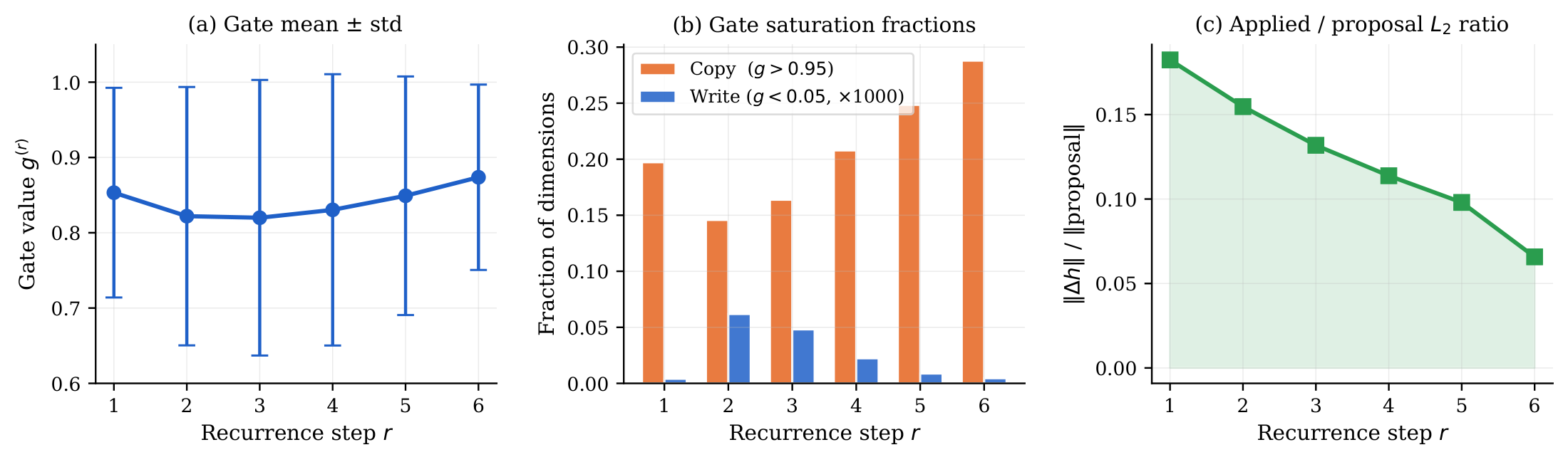
The gate transitions from a write-heavy regime (steps 1–2, mean $\approx 0.82$)
  to a copy-heavy regime (steps 3–6, mean $\approx 0.87$), with effective gate
  openness declining monotonically from $0.18$ to $0.07$.

E.3 Update Dynamics: Diminishing Magnitude, Increasing Alignment

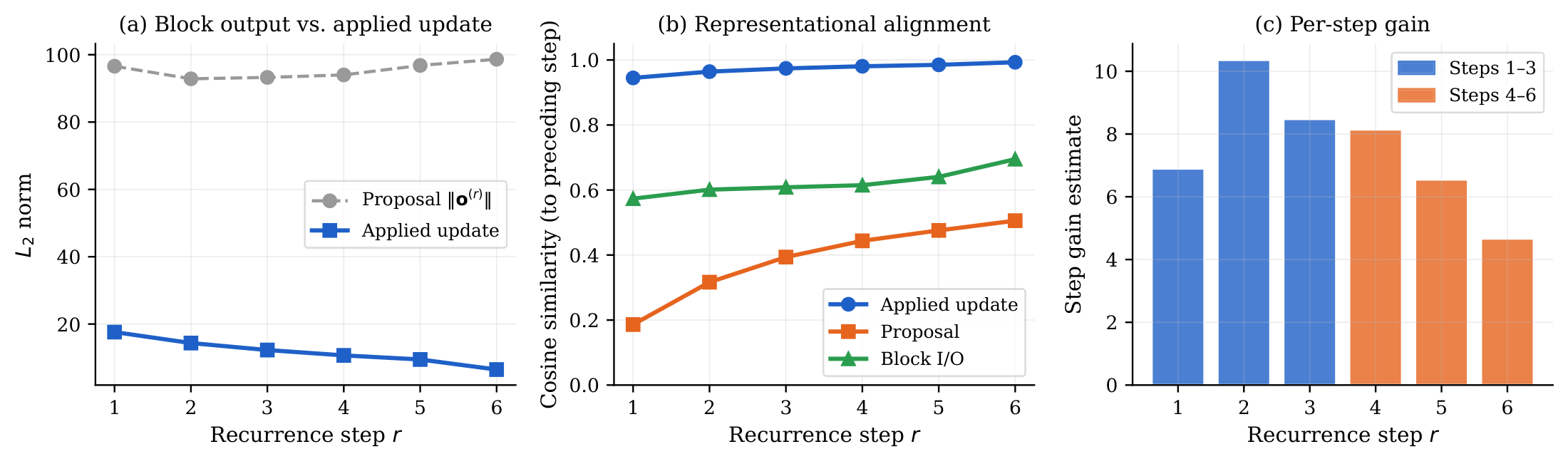
Figure 11(a) separates two quantities at each step: the $L_2$ norm of the shared block's raw proposal $\mathbf{o}^{(r)}$, and the $L_2$ norm of the gate-applied update that actually enters the residual stream. The proposal norms are nearly constant across all six steps ($93$ – $99$), possibly indicating that the shared block does not itself "know" it is being applied repeatedly—its output magnitude is stationary. The applied update, by contrast, declines from $17.6$ at step 1 to $6.5$ at step 6, driven entirely by the gate becoming more closed.

Figure 11(b) shows cosine similarity between successive representations, $\text{cos_sim}(\mathbf{h}^{r}, \mathbf{h}^{r-1})=\frac{\mathbf{h}^{r} \cdot \mathbf{h}^{r-1}}{| \mathbf{h}^{r} | | \mathbf{h}^{r-1} |}$. The proposal cosine similarity grows from $0.19$ at step 1 to $0.51$ at step 6, indicating that the block and the hidden state increasingly agree on direction as the representation stabilises. The applied update cosine similarity is already high at step 1 ($0.94$) and approaches $0.99$ by step 6, confirming that late-step corrections are directionally consistent refinements.

The per-step gain estimate (Figure 11(c)) peaks at step 2 ($10.4$), declining to $4.7$ at step 6. This concave gain profile, in which the most productive computation occurs before representational alignment is achieved, is consistent with the loss convergence plots in Appendix E.1.

E.4 Representational Geometry: Two-Phase Structure

We use Centered Kernel Alignment (CKA; [42]) to compare hidden-state representations across recurrence steps and against the corresponding layer representations of the GPT-2 Large dense baseline.

Within-model CKA

(Figure 12(a)). The $7 \times 7$ CKA matrix reveals a two-phase structure. Representations at step 0 (prelude) and step 1 are nearly identical (CKA $= 0.996$), while both are sharply dissimilar from all subsequent steps (CKA $\approx 0.33$ – $0.65$ with steps $\geq 2$). Steps 2 through 6 form a tightly cohesive cluster (pairwise CKA $\geq 0.907$), within which similarity decreases only gradually with step distance. This suggests the model undergoes a representational phase transition between steps 1 and 2.

Cross-model CKA

(Figure 12(b)). Prelude and step 1 representations align maximally with the shallow layers of the baseline (peak at layer 2, CKA $= 0.993$), while steps 2 through 6 all peak at baseline layer 11 (CKA $= 0.97$ – $0.90$ declining). No recurrent step aligns strongly with the deep layers of the baseline (layers

gt;20$, CKA lt; 0.50$), confirming that recurrent depth compresses the computational path but does not replicate the later representational hierarchy of the dense model.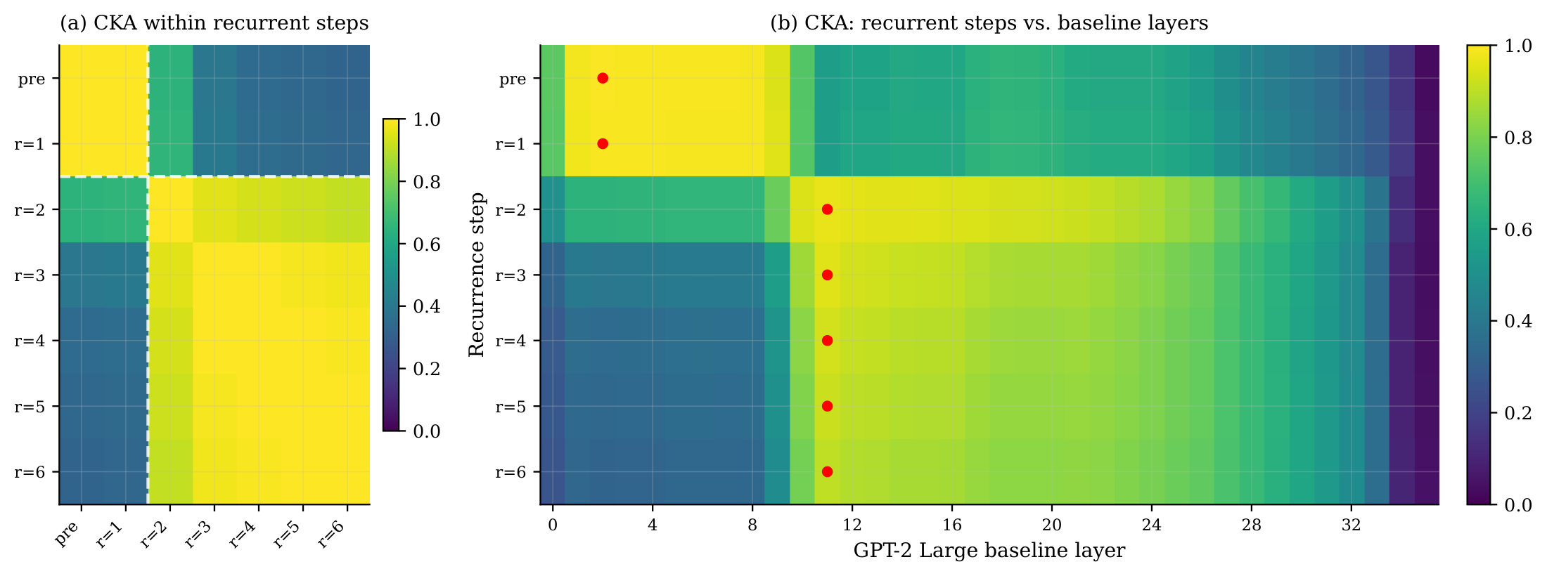

A representational phase transition occurs between steps 1 and 2: early steps
  resemble shallow baseline layers, while steps 2–6 all align with mid-depth
  baseline layer 11, compressing the computational path without replicating
  the deep-layer hierarchy.

E.5 Differential Routing by Token Difficulty

To test whether the gate allocates computation to where it is most needed, we sort tokens by their loss after the prelude (step 0) into ten deciles and track the total loss improvement accumulated over six recurrence steps. Figure 13(a) shows a near-linear relationship between initial token difficulty and total improvement ($R^2 = 0.998$): the easiest decile gains only $0.49$ nats, while the hardest decile gains $5.02$ nats—a ten-fold difference. The gate difficulty correlation—whether tokens with higher loss also receive lower (more open) gate values—is mildly negative across all steps ($-0.07$ to $-0.04$), consistent with the gate allowing slightly more writing for uncertain tokens.

E.6 Fixed-Point Convergence and Effective Rank

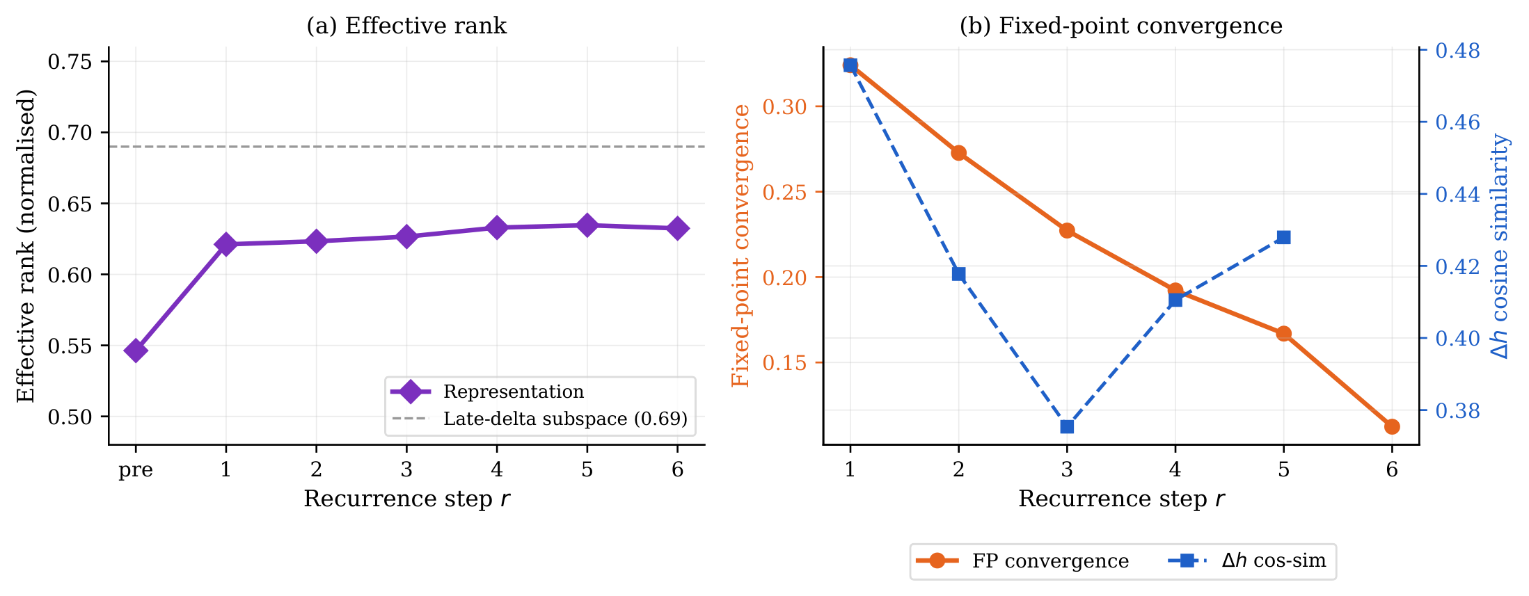
Figure 14(a) tracks the effective rank of the hidden-state tensor at each step. The rank increases from $0.546$ at the prelude to $0.635$ by step 3, after which it plateaus, indicating that iterative updates progressively spread information across more hidden dimensions. The effective rank of the delta subspace—the directions along which the hidden state changes in later steps—is $0.69$, higher than the rank of the representation itself, suggesting that late-step updates refine a diverse set of features.

Figure 14(b) plots the normalised fixed-point convergence metric, defined as

$ \delta_{\text{fp}}^{(r)} = \frac{| \mathbf{h}^{(r)} - \mathbf{h}^{(r-1)}|_F}{| \mathbf{h}^{(r-1)}|_F},\tag{4} $

the Frobenius-norm magnitude of the update relative to the current representation, which declines monotonically from $0.324$ at step 1 to $0.112$ at step 6, confirming that the recurrent dynamics are contractive.

Table 11 reports a sanity check via anchor ablations—swapping the fixed prelude output $\mathbf{h}^{(\mathrm{pre})}$ fed at each recurrence step for alternative anchors while keeping the gate and blocks identical. Crucially, the "previous hidden state" row uses $\mathbf{h}^{(r-1)}$ as anchor (i.e. the anchor drifts with the recurrence rather than being held fixed), while the learned gate remains fully active and adaptive. The $0.70$-nat gap between this condition ($3.38$) and the trained model ($2.68$) therefore quantifies the value of providing a stable, fixed reference point at every step, not merely the value of the gate.

\begin{tabular}{lcc}
  \toprule
  \textbf{Anchor type} & \textbf{Val. loss (nats)} & $\Delta$ vs. trained \\
  \midrule
  Zeros & 8.08 & +5.40 \\
  Input embedding & 3.73 & +1.05 \\
  Prev. hidden state $\mathbf{h}^{(r-1)}$ & 3.38 & +0.70 \\
  \midrule
  \textbf{Trained model} (fixed $\mathbf{h}^{(\mathrm{pre})}$) & \textbf{2.68} & --- \\
  \bottomrule
  \end{tabular}

E.7 Gate Attribution: Current State Gradually Supersedes the Anchor

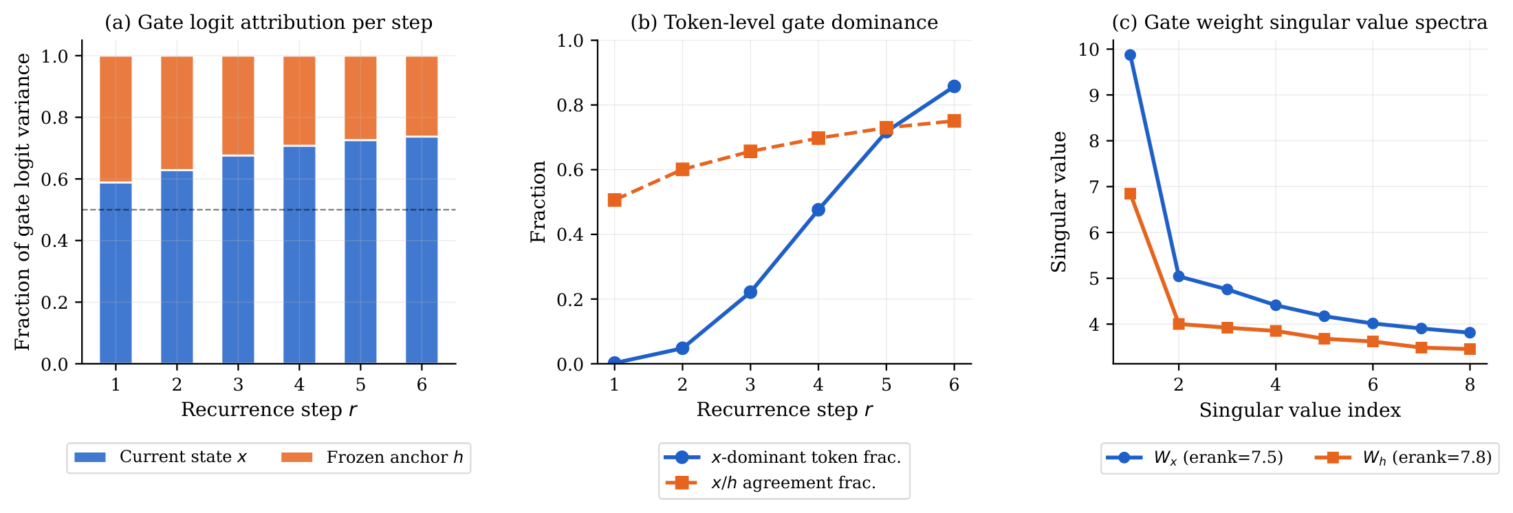
The elementwise ( reads from two sources simultaneously: $\hat{\mathbf{x}}^{(r)} \triangleq \mathrm{LN}(\mathbf{h}^{(r-1)})$, the LayerNorm-normalised current hidden state, [^1] and $\hat{\mathbf{h}} \triangleq \mathrm{LN}(\mathbf{h}^{(\mathrm{pre})})$, the normalised prelude anchor. The gate MLP $f_\mathbf{g}$ takes their concatenation as input; we write its first linear layer weight as $W_\mathbf{g} = [W_x \mid W_h] \in \mathbb{R}^{d_{\text{gate}} \times 2d}$, where $W_x \in \mathbb{R}^{d_{\text{gate}} \times d}$ acts on $\hat{\mathbf{x}}^{(r)}$ and $W_h \in \mathbb{R}^{d_{\text{gate}} \times d}$ acts on $\hat{\mathbf{h}}$. To quantify which source drives the gate at each step, we measure how much variance in the actual per-token gate logit each half explains. As seen in Figure 15(a), at step 1 the split is nearly even: 59% current state, 41% anchor. By step 6 this shifts substantially—74% current state, 26% anchor.

[^1]: We write $\hat{\mathbf{x}}^{(r)}$ rather than $x$ to avoid confusion with token IDs $(x_1, \ldots, x_S)$ introduced in the Preliminaries.

Figure 15(b) shows the same trend at the token level: the fraction of positions where the state half produces a larger absolute gate logit than the anchor grows from a near-zero 0.2% at step 1 to 86% at step 6. The answer to why is present in the weights before any forward pass: we find in Figure 15(c) that the leading singular value of $W_x$ is 9.87 versus 6.85 for $W_h$, giving the state half structurally greater sensitivity. At step 1 the hidden state is close to the prelude output, so the gap is small; as $x^{(r)}$ diverges from $h$ across steps, this structural asymmetry is amplified into the monotone attribution shift in Figure 15(a).

E.8 Projection Weight Analysis: State and Anchor as Complements

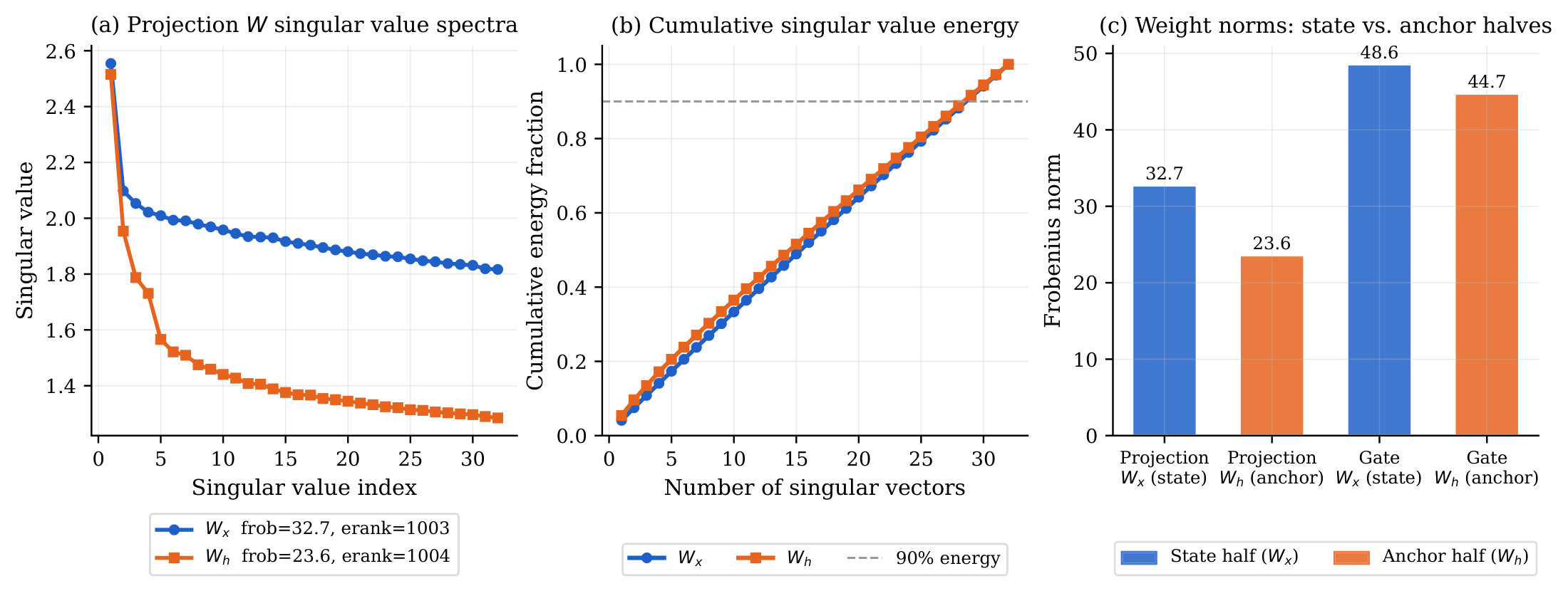
Before the shared blocks run, the recurrent projection, $W_{\text{proj}}$, maps the concatenated $[x^{(r)}, , h]$ into the $d$-dimensional input the transformer sees. A natural question is whether this projection simply averages the two sources or treats them as carrying distinct information. The answer is unambiguous: the mean row-wise cosine similarity between the $W_x$ and $W_h$ halves is $\mathbf{-0.189}$, with only $0.16%$ of the 1024 rows aligned above a cosine of $0.5$.

Both halves are nearly full-rank (effective ranks 1002.9 and 1004.3, Frobenius norms 32.7 and 23.6), with flat, slowly-decaying singular value spectra (Figure 16(a)–(b)). The negative mean row cosine means the projection reads the difference between current state and anchor rather than their average; we call this the contrastive projection property. Directions large in both $x^{(r)}$ and $h$ —stable features unchanged since the prelude—partially cancel; directions large only in $x^{(r)}$ are amplified. This provides a direct mechanistic explanation for why the fixed prelude is helpful: it supplies the reference needed to compute what has changed.

E.9 Attention Entropy: Stable Head Specialisations, Gradual Sharpening

Because identical weights govern every recurrence step, the shared block cannot self-modulate its attention patterns—any change must arise purely from changes in $\mathbf{h}^{(r)}$. In Figure 17(a), we capture the full $[B, n_\text{head}, S, S]$ attention tensors at each step (where $B$ is batch size and $n_\text{head}$ the number of attention heads) across all five shared blocks (100 heads total) and measure per-head Shannon entropy and diagonal mass.

Aggregate trend.

Mean attention entropy declines from 3.00 nats at step 1 to 2.77 at step 4, then rebounds to 2.82 at steps 5–6 (Figure 17(b)). This non-monotone profile mirrors the two-phase CKA structure from Appendix E.4: steps 1–4 are the refinement phase (lower entropy, more peaked patterns), while the rebound at steps 5–6 aligns with the final convergence plateau where small corrective updates scan broadly. Mean diagonal mass peaks at step 4 (0.108) then drops to 0.092 at step 6.

Head role stability.

The full $6 \times 100$ entropy heatmap (Figure 17(a)) makes the dominant pattern immediately visible: individual heads retain their character across all six steps. Of 100 heads, 2 are local/sharp (entropy

lt; 1.0$), 3 are previous-token (prev-mass gt; 0.35$), 2 are self-attention (diagonal mass gt; 0.35$), 7 are broad broadcast (entropy gt; 4.0$), and 86 are general. Here, prev-mass denotes the fraction of total attention weight placed on the immediately preceding token position (i.e. diagonal offset $-1$ of the attention matrix), averaged over the sequence. A head with prev-mass gt; 0.35$ predominantly attends to the token immediately before each query position. The clearest specialist—Block 0, Head 14—has entropy $0.298$ and prev-mass $0.878$ at step $r=1$,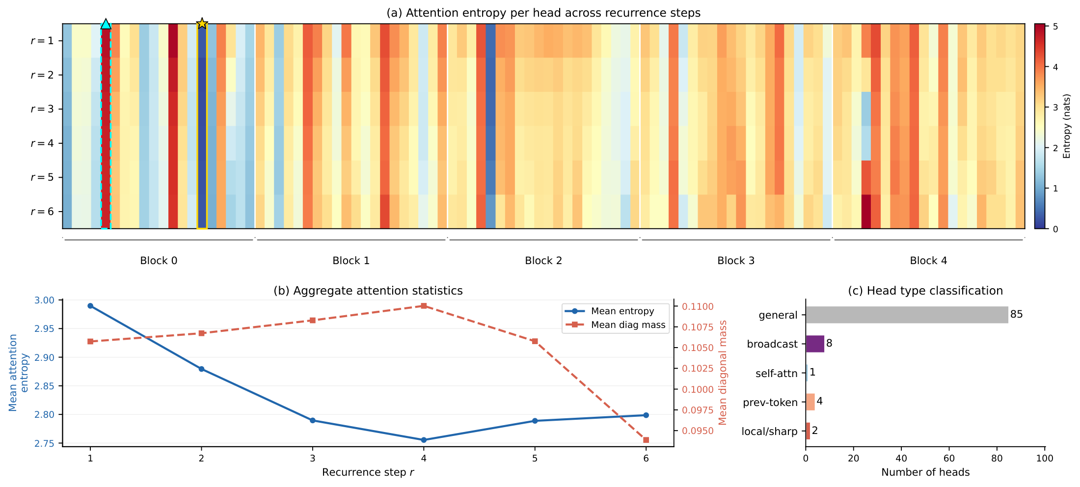

Head specialisations are locked in by weight and do not adapt to recurrence
  depth. What changes across steps is only the magnitude of each head's
  contribution, modulated by the gated update to the hidden state.

E.10 Recurrence Preferentially Serves Two Token Regimes

We split tokens into four BPE frequency bands: byte/punctuation (IDs 0–255, $n=5{,}763$), common (IDs 256–2,000, $n=15{,}789$), medium (IDs 2,001–10,000, $n=6{,}778$), and rare (IDs

gt;10{,}000$, $n=4{,}438$), where $n$ refers to the total occurrences of corresponding token id ranges in the validation set. Figure 18(a) shows that all four follow the familiar front-loaded loss-reduction profile, but at very different absolute scales: byte/punctuation tokens improve by just 1.92 nats while rare tokens improve by 3.39 nats.

Figure 18(b) plots the per-step relative improvement $\Delta_r^{\mathrm{rel}} = (L^{(r-1)} - L^{(r)}) / L^{(r-1)}$, i.e.\ the fraction of the preceding step's loss resolved at each step. At step $r=1$, byte/punctuation tokens already resolve 49% of their previous loss, compared to 23–28% for the other bands—recurrence is disproportionately productive for easy tokens first. Gains diminish uniformly beyond step 3 (

lt; 4$ % for all bands), consistent with the fixed-point convergence of Appendix E.6. Cumulatively over all six steps, byte/punctuation achieves 67% recovery of its initial loss versus 42% for rare tokens. We call these two roles completion (sharpening already-likely token predictions) and lexical narrowing (progressively concentrating probability mass for hard tokens). Both operate simultaneously in the same forward pass, possible because the elementwise gate allocates computation per-position rather than globally—no explicit routing mechanism is required.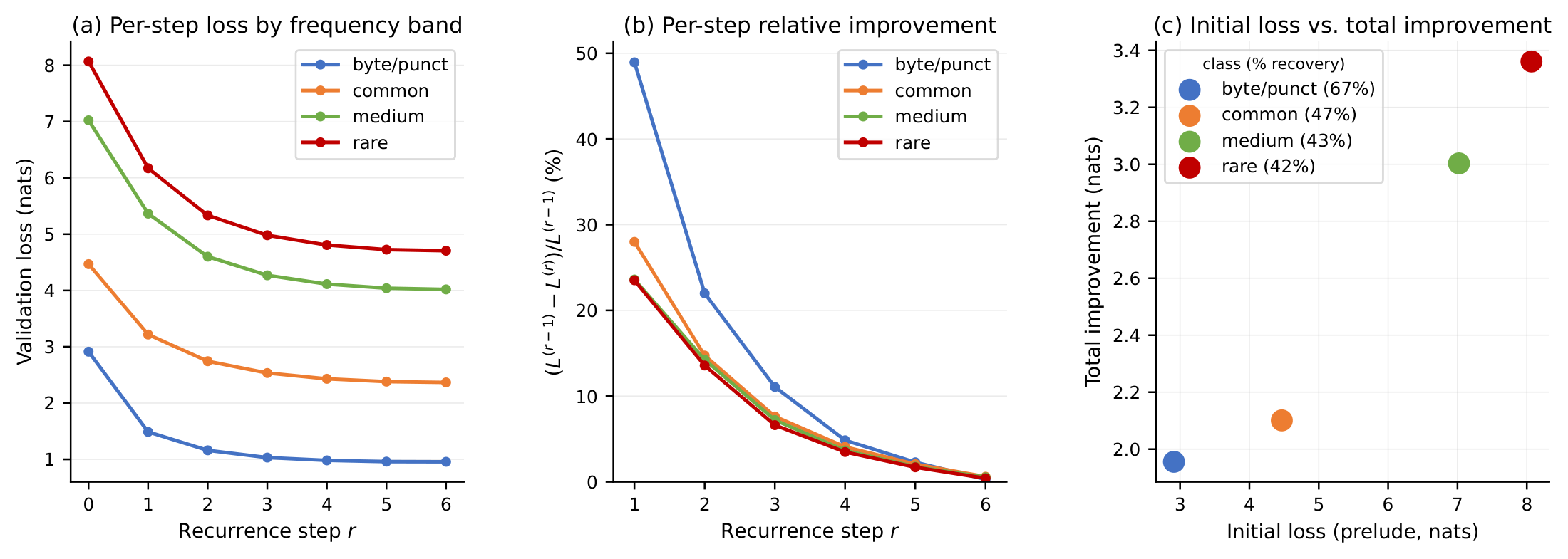

E.11 Unified Summary

The ten analyses above converge on a coherent computational and mechanistic account of how $\textsc{Gated Recurrent Transformer}$ 's shared block achieves its parameter efficiency.

Behaviourally, the model operates in two regimes separated by a representational phase transition between steps 1 and 2. In the early regime (steps 1–2), the gate is relatively open ($\approx 0.82$ mean, large update norms, high proposal cosine entropy), the hidden state undergoes a rapid restructuring that resolves $\sim$ 77% of predictive uncertainty, and CKA confirms a sharp departure from the prelude representation. In the late regime (steps 3–6), the gate progressively closes, updates shrink and align, the representation approaches a fixed point, and the attention patterns partially rebroadcast—consistent with targeted correction rather than coarse restructuring.

Mechanistically, four findings explain why this behaviour emerges from the learned weights. The gate weight asymmetry ($W_x$ leading singular values 44% larger than $W_h$) primes the gate to respond more strongly to changes in the hidden state than to the anchor, an advantage that is dynamically amplified as $x^{(r)}$ departs from $h$ across steps. The contrastive projection (mean row cosine $-0.19$) ensures the shared block receives an input that emphasises what has changed since the prelude, giving each step access to a difference signal rather than a raw state. The head specialisations are fixed by weight—the same 14 previous-token heads, 8 broadcast heads, and 11 self-attention heads appear at every step—so the block applies the same functional program each time; the gate, not the heads, decides how much of each step's output to incorporate. Finally, the token frequency breakdown reveals that a single forward pass simultaneously performs completion for common tokens and lexical narrowing for rare ones, made possible because the elementwise gate implicitly routes computation per-position without any explicit routing mechanism.

References

Section Summary: The references section lists dozens of academic papers and articles that underpin a discussion of neural language models, their scaling behavior, and techniques for improving reasoning through added computation or architectural tweaks. Spanning foundational works like Turing’s 1936 paper and early neural-network research through recent 2025–2026 studies on recurrent transformers and test-time scaling, the citations draw from arXiv preprints, conference proceedings, and journals such as Nature. Together they trace the evolution from classic recurrent models to modern methods that aim to make large language models more efficient reasoners.

[1] Jared Kaplan et al. (2020). Scaling Laws for Neural Language Models. https://arxiv.org/abs/2001.08361. arXiv:2001.08361.

[2] Alan Turing (1936). On Computable Numbers, with an Application to the Entscheidungsproblem. Proceedings of the London Mathematical Society. 42(1). pp. 230–265. doi:10.2307/2268810.

[3] Charlie Victor Snell et al. (2025). Scaling LLM Test-Time Compute Optimally Can be More Effective than Scaling Parameters for Reasoning. In The Thirteenth International Conference on Learning Representations. https://openreview.net/forum?id=4FWAwZtd2n.

[4] Learning to Reason with LLMs. https://openai.com/index/learning-to-reason-with-llms/.

[5] Guo et al. (2025). DeepSeek-R1 incentivizes reasoning in LLMs through reinforcement learning. Nature. 645(8081). pp. 633–638. doi:10.1038/s41586-025-09422-z. http://dx.doi.org/10.1038/s41586-025-09422-z.

[6] Guhao Feng et al. (2023). Towards Revealing the Mystery behind Chain of Thought: A Theoretical Perspective. In Thirty-seventh Conference on Neural Information Processing Systems. https://openreview.net/forum?id=qHrADgAdYu.

[7] Lan et al. (2020). ALBERT: A Lite BERT for Self-supervised Learning of Language Representations. In International Conference on Learning Representations.

[8] Mostafa Dehghani et al. (2019). Universal Transformers. In International Conference on Learning Representations. https://openreview.net/forum?id=HyzdRiR9Y7.

[9] Jonas Geiping et al. (2025). Scaling up Test-Time Compute with Latent Reasoning: A Recurrent Depth Approach. https://arxiv.org/abs/2502.05171. arXiv:2502.05171.

[10] Rui-Jie Zhu et al. (2025). Scaling Latent Reasoning via Looped Language Models. https://arxiv.org/abs/2510.25741. arXiv:2510.25741.

[11] Ahmadreza Jeddi et al. (2026). LoopFormer: Elastic-Depth Looped Transformers for Latent Reasoning via Shortcut Modulation. In The Fourteenth International Conference on Learning Representations. https://openreview.net/forum?id=RzYXb5YWBs.

[12] Sangmin Bae et al. (2025). Relaxed Recursive Transformers: Effective Parameter Sharing with Layer-wise LoRA. In The Thirteenth International Conference on Learning Representations. https://openreview.net/forum?id=WwpYSOkkCt.

[13] Bolya, Daniel and others (2025). Depth as Modulation in Weight-Sharing Transformers. In The Thirteenth International Conference on Learning Representations. https://openreview.net/forum?id=wm9jRInse3.

[14] Rumelhart et al. (1986). Learning representations by back-propagating errors. Nature. 323. pp. 533–536. doi:10.1038/323533a0.

[15] Werbos, P.J. (1990). Backpropagation through time: what it does and how to do it. Proceedings of the IEEE. 78(10). pp. 1550-1560. doi:10.1109/5.58337.

[16] Elman, Jeffrey L. (1990). Finding Structure in Time. Cognitive Science. 14(2). pp. 179-211. doi:https://doi.org/10.1207/s15516709cog140$2_1. $https://onlinelibrary.wiley.com/doi/abs/10.1207/s15516709cog140$2_1$.

[17] Hochreiter, Sepp and Schmidhuber, Jürgen (1997). Long Short-Term Memory. Neural Computation. 9(8). pp. 1735-1780. doi:10.1162/neco.1997.9.8.1735.

[18] Cho et al. (2014). Learning Phrase Representations using RNN Encoder–Decoder for Statistical Machine Translation. In Proceedings of the 2014 Conference on Empirical Methods in Natural Language Processing (EMNLP). pp. 1724–1734. doi:10.3115/v1/D14-1179. https://aclanthology.org/D14-1179/.

[19] Devlin et al. (2019). BERT: Pre-training of Deep Bidirectional Transformers for Language Understanding. In Proceedings of the 2019 Conference of the North American Chapter of the Association for Computational Linguistics: Human Language Technologies, Volume 1 (Long and Short Papers). pp. 4171–4186. doi:10.18653/v1/N19-1423. https://aclanthology.org/N19-1423/.

[20] Yeskendir Koishekenov et al. (2025). Encode, Think, Decode: Scaling test-time reasoning with recursive latent thoughts. https://arxiv.org/abs/2510.07358. arXiv:2510.07358.

[21] Geva et al. (2021). Transformer Feed-Forward Layers Are Key-Value Memories. In Proceedings of the 2021 Conference on Empirical Methods in Natural Language Processing. pp. 5484–5495. doi:10.18653/v1/2021.emnlp-main.446. https://aclanthology.org/2021.emnlp-main.446/.

[22] Ruike Zhu et al. (2025). Beyond Parameters: Exploring Virtual Logic Depth for Scaling Laws. https://arxiv.org/abs/2506.18233. arXiv:2506.18233.

[23] Alex Graves (2017). Adaptive Computation Time for Recurrent Neural Networks. https://arxiv.org/abs/1603.08983. arXiv:1603.08983.

[24] David Raposo et al. (2024). Mixture-of-Depths: Dynamically allocating compute in transformer-based language models. https://arxiv.org/abs/2404.02258. arXiv:2404.02258.

[25] Sangmin Bae et al. (2026). Mixture-of-Recursions: Learning Dynamic Recursive Depths for Adaptive Token-Level Computation. In The Thirty-ninth Annual Conference on Neural Information Processing Systems. https://openreview.net/forum?id=QuqsEIVWIG.

[26] Shaojie Bai et al. (2019). Deep Equilibrium Models. In Advances in Neural Information Processing Systems.

[27] Jordan Hoffmann et al. (2022). Training Compute-Optimal Large Language Models. https://arxiv.org/abs/2203.15556. arXiv:2203.15556.

[28] Stella Biderman et al. (2023). Pythia: A Suite for Analyzing Large Language Models Across Training and Scaling. https://arxiv.org/abs/2304.01373. arXiv:2304.01373.

[29] Gilad Yehudai et al. (2026). Depth-Width tradeoffs in Algorithmic Reasoning of Graph Tasks with Transformers. https://arxiv.org/abs/2503.01805. arXiv:2503.01805.

[30] Sean Michael McLeish et al. (2026). Gemstones: A Model Suite for Multi-Faceted Scaling Laws. In The Thirty-ninth Annual Conference on Neural Information Processing Systems. https://openreview.net/forum?id=iZk78dZ1Ap.

[31] Jimmy Lei Ba et al. (2016). Layer Normalization. https://arxiv.org/abs/1607.06450. arXiv:1607.06450.

[32] Gers et al. (2000). Learning to Forget: Continual Prediction with LSTM. Neural Computation. 12(10). pp. 2451–2471.

[33] Jozefowicz et al. (2015). An Empirical Exploration of Recurrent Network Architectures. In Proceedings of the 32nd International Conference on Machine Learning. pp. 2342–2350.

[34] Google DeepMind (2025). Gemma 3n Model Overview. https://ai.google.dev/gemma/docs/gemma-3n. Introduced Per-Layer Embeddings (PLE) for on-device LLMs.

[35] Google DeepMind (2026). Gemma 4 Model Overview. https://ai.google.dev/gemma/docs/core. Accessed: 2026-05-06. Last updated 2026-04-16.

[36] Yanxi Chen et al. (2024). EE-LLM: Large-Scale Training and Inference of Early-Exit Large Language Models with 3D Parallelism. In The Forty-first International Conference on Machine Learning.

[37] Elhoushi et al. (2024). LayerSkip: Enabling Early Exit Inference and Self-Speculative Decoding. In Proceedings of the 62nd Annual Meeting of the Association for Computational Linguistics (Volume 1: Long Papers). pp. 12622–12642. doi:10.18653/v1/2024.acl-long.681. https://aclanthology.org/2024.acl-long.681/.

[38] Karpathy, Andrej (2022). NanoGPT. https://github.com/karpathy/nanoGPT.

[39] Loshchilov, Ilya and Hutter, Frank (2019). Decoupled Weight Decay Regularization. In International Conference on Learning Representations.

[40] Radford et al. (2019). Language Models are Unsupervised Multitask Learners.

[41] Gao et al. (2024). The Language Model Evaluation Harness. doi:10.5281/zenodo.12608602. https://zenodo.org/records/12608602.

[42] Kornblith et al. (2019). Similarity of Neural Network Representations Revisited. In Proceedings of the 36th International Conference on Machine Learning. pp. 3519–3529.