Simplifying Graph Convolutional Networks

Felix Wu$^{,1}$, Tianyi Zhang$^{,1}$, Amauri Holanda de Souza Jr.$^{*,1,2}$, Christopher Fifty$^{1}$, Tao Yu$^{1}$, Kilian Q. Weinberger$^{1}$

$^{*}$Equal contribution

$^{1}$Cornell University

$^{2}$Federal Institute of Ceara (Brazil).

Correspondence to: Felix Wu [email protected], Tianyi Zhang [email protected].Proceedings of the $36^{\text{th}}$ International Conference on Machine Learning, Long Beach, California, PMLR 97, 2019. Copyright 2019 by the author(s).

Abstract

Graph Convolutional Networks (GCNs) and their variants have experienced significant attention and have become the de facto methods for learning graph representations. GCNs derive inspiration primarily from recent deep learning approaches, and as a result, may inherit unnecessary complexity and redundant computation. In this paper, we reduce this excess complexity through successively removing nonlinearities and collapsing weight matrices between consecutive layers. We theoretically analyze the resulting linear model and show that it corresponds to a fixed low-pass filter followed by a linear classifier. Notably, our experimental evaluation demonstrates that these simplifications do not negatively impact accuracy in many downstream applications. Moreover, the resulting model scales to larger datasets, is naturally interpretable, and yields up to two orders of magnitude speedup over FastGCN.

Executive Summary: Graph convolutional networks (GCNs) have become standard tools for analyzing data structured as graphs, such as social networks, citation databases, and molecular structures. These networks help predict node labels, like classifying research papers by topic or identifying user communities, by propagating information across connections. However, GCNs often incorporate layers of nonlinear transformations borrowed from deep learning, adding computational cost and reducing interpretability. With growing graph sizes in real-world applications, from recommendation systems to drug discovery, there is urgent need for simpler, faster models that preserve accuracy without unnecessary complexity.

This paper aims to derive and evaluate the simplest linear version of a GCN, called Simple Graph Convolution (SGC), by stripping away nonlinearities and collapsing multi-layer operations into a single transformation. It seeks to test whether this reduction harms performance or offers benefits in speed and clarity.

The authors conducted a theoretical analysis of the simplified model and ran experiments on benchmark datasets for node classification, including citation networks (Cora with 2,700 nodes, CiteSeer with 3,300 nodes, and PubMed with 19,700 nodes) and the larger Reddit social network (233,000 nodes). They also applied SGC to downstream tasks using public datasets for text classification, user geolocation, relation extraction, and zero-shot image classification. Key assumptions included sparse graph connectivity and the use of a "renormalization trick" (adding self-loops to edges) to stabilize propagation. Comparisons involved reimplementing or using code from baselines like standard GCNs, Graph Attention Networks (GATs), and FastGCN.

The core findings highlight SGC's effectiveness. First, SGC achieves test accuracies comparable to or slightly better than full GCNs on citation networks—81.0% versus 81.4% on Cora and 71.9% versus 70.9% on CiteSeer—while using far fewer parameters and avoiding overfitting. Second, it outperforms sampling-based methods like FastGCN by over 1% on Reddit (94.9% F1 score) and scales to this 233,000-node graph without memory issues. Third, theoretically, SGC acts as a fixed low-pass filter that smooths features across connected nodes, followed by a simple linear classifier, making it highly interpretable. Fourth, on downstream tasks, SGC rivals or exceeds GCN variants, such as 88.5% accuracy on 20 Newsgroups text classification (versus 87.9%) and 67.0% on relation extraction (versus 66.4%), often with 50-80 times faster training.

These results imply that the power of GCNs stems mainly from graph propagation rather than nonlinear layers, challenging assumptions in deep graph learning. For practitioners, SGC reduces computational costs dramatically—up to 100 times speedup on large graphs—lowering risks of resource-intensive training and enabling deployment on modest hardware. It enhances interpretability, aiding compliance in sensitive areas like social media analysis, and performs well even with limited labels, improving semi-supervised learning efficiency. Unlike expectations that deeper nonlinear models are essential, SGC shows simplicity can match complexity here, potentially simplifying policy for graph AI adoption.

Leaders should adopt SGC as an initial model for node classification and related tasks, especially on large or sparse graphs, and use it as a baseline for evaluating new methods. For broader applications, integrate it into pipelines for text or image tasks, weighing its speed against needs for high expressivity (e.g., pair with MLPs where needed). Further pilots on domain-specific graphs, like biological networks, would confirm generalizability; if results hold, prioritize it over complex GCNs to cut timelines and costs.

While confident in SGC's strengths for the tested scenarios—supported by consistent outperformance across datasets—limitations include potential underperformance on dense graphs or tasks requiring nuanced feature hierarchies, such as quantum chemistry prediction, where advanced models scored 3-4 times better. Data from 2017-2019 benchmarks may not capture newer graph types, so caution applies to evolving real-world data; additional validation on fresh datasets is advised.

1. Introduction

Section Summary: Graph Convolutional Networks, or GCNs, are a type of neural network designed for analyzing graph-structured data like social or citation networks, where they have excelled in tasks from chemistry to computer vision by layering filters and activations to learn useful patterns. However, unlike most machine learning tools that start simple and grow complex only when necessary, GCNs were built overly intricate from the outset, prompting researchers to create a streamlined alternative called Simple Graph Convolution, or SGC, which removes nonlinear steps to form a basic linear model. This SGC matches or beats GCN performance across various benchmarks while running much faster, using fewer resources, and offering clearer insights into how it processes graph data.

Graph Convolutional Networks (GCNs) [1] are an efficient variant of Convolutional Neural Networks (CNNs) on graphs. GCNs stack layers of learned first-order spectral filters followed by a nonlinear activation function to learn graph representations. Recently, GCNs and subsequent variants have achieved state-of-the-art results in various application areas, including but not limited to citation networks [1], social networks [2], applied chemistry [3], natural language processing [4, 5, 6], and computer vision [7, 8].

Historically, the development of machine learning algorithms has followed a clear trend from initial simplicity to need-driven complexity. For instance, limitations of the linear Perceptron [9] motivated the development of the more complex but also more expressive neural network (or multi-layer Perceptrons, MLPs) [10]. Similarly, simple pre-defined linear image filters [11, 12] eventually gave rise to nonlinear CNNs with learned convolutional kernels [13, 14]. As additional algorithmic complexity tends to complicate theoretical analysis and obfuscates understanding, it is typically only introduced for applications where simpler methods are insufficient. Arguably, most classifiers in real world applications are still linear (typically logistic regression), which are straight-forward to optimize and easy to interpret.

However, possibly because GCNs were proposed after the recent "renaissance" of neural networks, they tend to be a rare exception to this trend. GCNs are built upon multi-layer neural networks, and were never an extension of a simpler (insufficient) linear counterpart.

In this paper, we observe that GCNs inherit considerable complexity from their deep learning lineage, which can be burdensome and unnecessary for less demanding applications. Motivated by the glaring historic omission of a simpler predecessor, we aim to derive the simplest linear model that ``could have" preceded the GCN, had a more "traditional" path been taken. We reduce the excess complexity of GCNs by repeatedly removing the nonlinearities between GCN layers and collapsing the resulting function into a single linear transformation. We empirically show that the final linear model exhibits comparable or even superior performance to GCNs on a variety of tasks while being computationally more efficient and fitting significantly fewer parameters. We refer to this simplified linear model as Simple Graph Convolution (SGC).

In contrast to its nonlinear counterparts, the SGC is intuitively interpretable and we provide a theoretical analysis from the graph convolution perspective. Notably, feature extraction in SGC corresponds to a single fixed filter applied to each feature dimension. [1] empirically observe that the "renormalization trick", i.e. adding self-loops to the graph, improves accuracy, and we demonstrate that this method effectively shrinks the graph spectral domain, resulting in a low-pass-type filter when applied to SGC. Crucially, this filtering operation gives rise to locally smooth features across the graph [15].

Through an empirical assessment on node classification benchmark datasets for citation and social networks, we show that the SGC achieves comparable performance to GCN and other state-of-the-art graph neural networks. However, it is significantly faster, and even outperforms FastGCN ([2]) by up to two orders of magnitude on the largest dataset (Reddit) in our evaluation. Finally, we demonstrate that SGC extrapolates its effectiveness to a wide-range of downstream tasks. In particular, SGC rivals, if not surpasses, GCN-based approaches on text classification, user geolocation, relation extraction, and zero-shot image classification tasks. The code is available on Github^1.

2. Simple Graph Convolution

Section Summary: Graph Convolutional Networks (GCNs) help classify nodes in a graph by taking node features and iteratively updating them across layers, where each layer averages a node's features with those of its neighbors to spread information along connections, then applies a linear transformation and a nonlinear activation like ReLU. This creates smoothed representations that encourage similar nearby nodes to have similar predictions, much like how image convolutions capture local patterns. The Simple Graph Convolution method simplifies this by removing the nonlinear steps between layers, arguing that the main power comes from the neighbor-averaging process itself, which expands a node's view to farther connections with more layers.

We follow [1] to introduce GCNs (and subsequently SGC) in the context of node classification. Here, GCNs take a graph with some labeled nodes as input and generate label predictions for all graph nodes. Let us formally define such a graph as ${\mathcal{G}} = ({\mathcal{V}}, {\mathbf{A}})$, where $\mathcal{V}$ represents the vertex set consisting of nodes ${v_1, \dots, v_n}$, and ${\mathbf{A}}\in\mathbb{R}^{n \times n}$ is a symmetric (typically sparse) adjacency matrix where $a_{ij}$ denotes the edge weight between nodes $v_i$ and $v_j$. A missing edge is represented through $a_{ij} = 0$. We define the degree matrix ${\mathbf{D}} = \text{diag}(d_1, \dots, d_n)$ as a diagonal matrix where each entry on the diagonal is equal to the row-sum of the adjacency matrix $d_i = \sum_j a_{ij}$.

Each node $v_i$ in the graph has a corresponding $d$-dimensional feature vector ${\mathbf{x}}_i \in \mathbb{R}^{d}$. The entire feature matrix ${\mathbf{X}} \in \mathbb{R}^{n \times d}$ stacks $n$ feature vectors on top of one another, ${\mathbf{X}}=\left[{\mathbf{x}}_1, \dots, {\mathbf{x}}_n\right]^\top$. Each node belongs to one out of $C$ classes and can be labeled with a $C$-dimensional one-hot vector ${\mathbf{y}}_i\in{0, 1}^C$. We only know the labels of a subset of the nodes and want to predict the unknown labels.

2.1 Graph Convolutional Networks

Similar to CNNs or MLPs, GCNs learn a new feature representation for the feature $\mathbf{x}_i$ of each node over multiple layers, which is subsequently used as input into a linear classifier. For the $k$-th graph convolution layer, we denote the input node representations of all nodes by the matrix $\mathbf{H}^{(k-1)}$ and the output node representations $\mathbf{H}^{(k)}$. Naturally, the initial node representations are just the original input features:

$ \mathbf{H}^{(0)} = \mathbf{X},\tag{1} $

which serve as input to the first GCN layer.

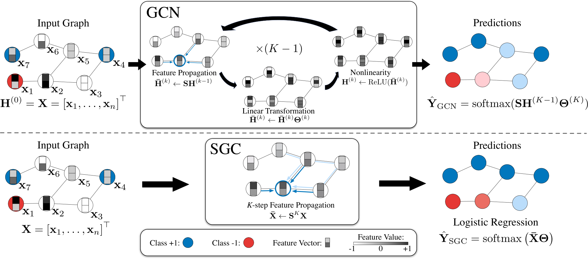
A $K$-layer GCN is identical to applying a $K$-layer MLP to the feature vector $\mathbf{x}_i$ of each node in the graph, except that the hidden representation of each node is averaged with its neighbors at the beginning of each layer. In each graph convolution layer, node representations are updated in three stages: feature propagation, linear transformation, and a pointwise nonlinear activation (see Figure 1). For the sake of clarity, we describe each step in detail.

Feature propagation

is what distinguishes a GCN from an MLP. At the beginning of each layer the features $\mathbf{h}_i$ of each node $v_i$ are averaged with the feature vectors in its local neighborhood,

$ \bar{\mathbf{h}}i^{(k)} \leftarrow \frac{1}{d_i + 1} \mathbf{h}i^{(k-1)}+\sum{j=1}^n \frac{a{ij}}{\sqrt{(d_i + 1) (d_j + 1)}}\mathbf{h}_j^{(k-1)}.\tag{2} $

More compactly, we can express this update over the entire graph as a simple matrix operation. Let ${\mathbf{S}}$ denote the ``normalized" adjacency matrix with added self-loops,

$ \begin{align} \mathbf{S} & = \tilde{{\mathbf{D}}}^{-\frac{1}{2}} \tilde{{\mathbf{A}}} \tilde{{\mathbf{D}}}^{-\frac{1}{2}}, \end{align}\tag{3} $

where $\tilde{{\mathbf{A}}} = {\mathbf{A}} + {\mathbf{I}}$ and $\tilde{{\mathbf{D}}}$ is the degree matrix of $\tilde{{\mathbf{A}}}$. The simultaneous update in Equation 2 for all nodes becomes a simple sparse matrix multiplication

$ \bar{\mathbf{H}}^{(k)} \leftarrow \mathbf{S} \mathbf{H}^{(k-1)}. $

Intuitively, this step smoothes the hidden representations locally along the edges of the graph and ultimately encourages similar predictions among locally connected nodes.

Feature transformation and nonlinear transition.

After the local smoothing, a GCN layer is identical to a standard MLP. Each layer is associated with a learned weight matrix $\boldsymbol{\Theta}^{(k)}$, and the smoothed hidden feature representations are transformed linearly. Finally, a nonlinear activation function such as $\mathrm{ReLU}$ is applied pointwise before outputting feature representation ${\mathbf{H}}^{(k)}$. In summary, the representation updating rule of the $k$-th layer is:

$ \begin{align} \mathbf{H}^{(k)} & \leftarrow \mathrm{ReLU} \left(\bar{\mathbf{H}}^{(k)} \boldsymbol{\Theta}^{(k)}\right). \end{align}\tag{4} $

The pointwise nonlinear transformation of the $k$-th layer is followed by the feature propagation of the $(k+1)$-th layer.

Classifier.

For node classification, and similar to a standard MLP, the last layer of a GCN predicts the labels using a softmax classifier. Denote the class predictions for $n$ nodes as $\hat{\mathbf{Y}} \in \mathbb{R}^{n\times C}$ where $\hat{y}_{ic}$ denotes the probability of node $i$ belongs to class $c$. The class prediction $\hat{\mathbf{Y}}$ of a $K$-layer GCN can be written as:

$ \begin{align} \hat{\mathbf{Y}}_{\text{GCN}} & = \mathrm{softmax}\left({\mathbf{S}} \mathbf{H}^{(K-1)} \boldsymbol{\Theta}^{(K)}\right), \end{align} $

where $\mathrm{softmax}({\mathbf{x}}) = \exp({\mathbf{x}}) / \sum_{c=1}^C \exp(x_c)$ acts as a normalizer across all classes.

2.2 Simple Graph Convolution

In a traditional MLP, deeper layers increase the expressivity because it allows the creation of feature hierarchies, e.g. features in the second layer build on top of the features of the first layer. In GCNs, the layers have a second important function: in each layer the hidden representations are averaged among neighbors that are one hop away. This implies that after $k$ layers a node obtains feature information from all nodes that are $k-$ hops away in the graph. This effect is similar to convolutional neural networks, where depth increases the receptive field of internal features [16]. Although convolutional networks can benefit substantially from increased depth [17], typically MLPs obtain little benefit beyond 3 or 4 layers.

Linearization.

We hypothesize that the nonlinearity between GCN layers is not critical - but that the majority of the benefit arises from the local averaging. We therefore remove the nonlinear transition functions between each layer and only keep the final softmax (in order to obtain probabilistic outputs). The resulting model is linear, but still has the same increased "receptive field" of a $K$-layer GCN,

$ \begin{align} \hat{\mathbf{Y}} & = \mathrm{softmax}\left(\mathbf{S}\ldots\mathbf{S}\mathbf{S} \mathbf{X} \boldsymbol{\Theta}^{(1)}\boldsymbol{\Theta}^{(2)}\ldots\boldsymbol{\Theta}^{(K)} \right). \end{align} $

To simplify notation we can collapse the repeated multiplication with the normalized adjacency matrix ${\mathbf{S}}$ into a single matrix by raising ${\mathbf{S}}$ to the $K$-th power, ${\mathbf{S}}^K$. Further, we can reparameterize our weights into a single matrix $\boldsymbol{\Theta}=\boldsymbol{\Theta}^{(1)} \boldsymbol{\Theta}^{(2)} \ldots \boldsymbol{\Theta}^{(K)}$. The resulting classifier becomes

$ \hat{\mathbf{Y}}_{\text{SGC}}= \mathrm{softmax}\left(\mathbf{S}^K \mathbf{X} \boldsymbol{\Theta} \right),\tag{5} $

which we refer to as Simple Graph Convolution (SGC).

Logistic regression.

Equation 5 gives rise to a natural and intuitive interpretation of SGC: by distinguishing between feature extraction and classifier, SGC consists of a fixed (i.e., parameter-free) feature extraction/smoothing component $\bar{{\mathbf{X}}}= {\mathbf{S}}^K {\mathbf{X}}$ followed by a linear logistic regression classifier $\hat{\mathbf{Y}}= \mathrm{softmax}(\bar{{\mathbf{X}}}\boldsymbol{\Theta})$. Since the computation of $\bar{{\mathbf{X}}}$ requires no weight it is essentially equivalent to a feature pre-processing step and the entire training of the model reduces to straight-forward multi-class logistic regression on the pre-processed features $\bar {\mathbf{X}}$.

Optimization details.

The training of logistic regression is a well studied convex optimization problem and can be performed with any efficient second order method or stochastic gradient descent [18]. Provided the graph connectivity pattern is sufficiently sparse, SGD naturally scales to very large graph sizes and the training of SGC is drastically faster than that of GCNs.

3. Spectral Analysis

Section Summary: This section examines the Simplified Graph Convolution (SGC) method through the lens of graph spectral analysis, showing that it applies a fixed filter in the graph's frequency domain to process node features. By adding self-loops to the graph—a technique called the renormalization trick—the method scales down the graph's spectrum, turning SGC into a low-pass filter that smooths features across connected nodes. As a result, nearby nodes end up with similar representations, leading to more consistent predictions.

We now study SGC from a graph convolution perspective. We demonstrate that SGC corresponds to a fixed filter on the graph spectral domain. In addition, we show that adding self-loops to the original graph, i.e. the renormalization trick ([1]), effectively shrinks the underlying graph spectrum. On this scaled domain, SGC acts as a low-pass filter that produces smooth features over the graph. As a result, nearby nodes tend to share similar representations and consequently predictions.

3.1 Preliminaries on Graph Convolutions

Analogous to the Euclidean domain, graph Fourier analysis relies on the spectral decomposition of graph Laplacians. The graph Laplacian $\boldsymbol{\Delta} = {\mathbf{D}} - {\mathbf{A}}$ (as well as its normalized version $\boldsymbol{\Delta}_{\text{sym}} = {\mathbf{D}}^{-1/2}\boldsymbol{\Delta} {\mathbf{D}}^{-1/2}$) is a symmetric positive semidefinite matrix with eigendecomposition $\boldsymbol{\Delta} = {\mathbf{U}} \boldsymbol{\Lambda} {\mathbf{U}}^{\top}$, where ${\mathbf{U}} \in \mathbb{R}^{n \times n}$ comprises orthonormal eigenvectors and $\boldsymbol{\Lambda} = \text{diag}(\lambda_1, \dots, \lambda_n)$ is a diagonal matrix of eigenvalues. The eigendecomposition of the Laplacian allows us to define the Fourier transform equivalent on the graph domain, where eigenvectors denote Fourier modes and eigenvalues denote frequencies of the graph. In this regard, let ${\mathbf{x}} \in \mathbb{R}^n$ be a signal defined on the vertices of the graph. We define the graph Fourier transform of ${\mathbf{x}}$ as $\hat{{\mathbf{x}}} = {\mathbf{U}}^{\top}{\mathbf{x}}$, with inverse operation given by ${\mathbf{x}} = {\mathbf{U}} \hat{{\mathbf{x}}}$. Thus, the graph convolution operation between signal ${\mathbf{x}}$ and filter ${\mathbf{g}}$ is

$ {\mathbf{g}} * {\mathbf{x}} = {\mathbf{U}} \left(({\mathbf{U}}^\top {\mathbf{g}}) \odot ({\mathbf{U}}^\top {\mathbf{x}}) \right) = {\mathbf{U}} \hat{{\mathbf{G}}} {\mathbf{U}}^\top {\mathbf{x}},\tag{6} $

where $\hat{{\mathbf{G}}} = \text{diag}\left(\hat{g}_1, \dots, \hat{g}_n\right)$ denotes a diagonal matrix in which the diagonal corresponds to spectral filter coefficients.

Graph convolutions can be approximated by $k$-th order polynomials of Laplacians

$ {\mathbf{U}}\hat{{\mathbf{G}}}{\mathbf{U}}^\top {\mathbf{x}} \approx \sum_{i=0}^{k} \theta_i \boldsymbol{\Delta}^i {\mathbf{x}} = {\mathbf{U}} \left(\sum_{i=0}^{k} \theta_i \boldsymbol{\Lambda}^i \right) {\mathbf{U}}^\top {\mathbf{x}},\tag{7} $

where $\theta_i$ denotes coefficients. In this case, filter coefficients correspond to polynomials of the Laplacian eigenvalues, i.e., $\hat{{\mathbf{G}}} = \sum_i \theta_i \boldsymbol{\Lambda}^i$ or equivalently $\hat{g}(\lambda_j) = \sum_i \theta_i \lambda_j^i$.

Graph Convolutional Networks (GCNs) [1] employ an affine approximation ($k=1$) of [@eq:polynomial_approximation] with coefficients $\theta_0=2\theta$ and $\theta_1=-\theta$ from which we attain the basic GCN convolution operation

$ {\mathbf{g}} * {\mathbf{x}} = \theta ({\mathbf{I}} + {\mathbf{D}}^{-1/2} {\mathbf{A}} {\mathbf{D}}^{-1/2}) {\mathbf{x}}.\tag{8} $

In their final design, [1] replace the matrix ${\mathbf{I}} + {\mathbf{D}}^{-1/2} {\mathbf{A}} {\mathbf{D}}^{-1/2}$ by a normalized version $\tilde{{\mathbf{D}}}^{-1/2} \tilde{{\mathbf{A}}} \tilde{{\mathbf{D}}}^{-1/2}$ where $\tilde{{\mathbf{A}}} = {\mathbf{A}} + {\mathbf{I}}$ and consequently $\tilde{{\mathbf{D}}} = {\mathbf{D}} + {\mathbf{I}}$, dubbed the renormalization trick. Finally, by generalizing the convolution to work with multiple filters in a $d$-channel input and layering the model with nonlinear activation functions between each layer, we have the GCN propagation rule as defined in Equation 4.

3.2 SGC and Low-Pass Filtering

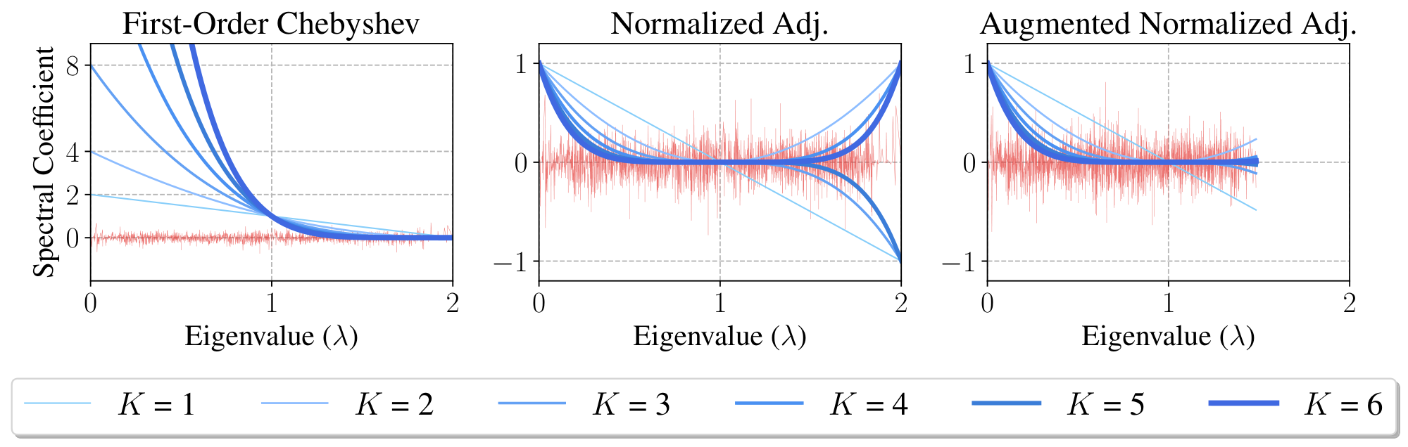
The initial first-order Chebyshev filter derived in GCNs corresponds to the propagation matrix ${\mathbf{S}}{\text{1-order}} = {\mathbf{I}} + {\mathbf{D}}^{-1/2} {\mathbf{A}} {\mathbf{D}}^{-1/2}$ (see Equation 8). Since the normalized Laplacian is $\boldsymbol{\Delta}{\text{sym}} = {\mathbf{I}} - {\mathbf{D}}^{-1/2} {\mathbf{A}} {\mathbf{D}}^{-1/2}$, then ${\mathbf{S}}{\text{1-order}} = 2 {\mathbf{I}} - \boldsymbol{\Delta}{\text{sym}}$. Therefore, feature propagation with ${\mathbf{S}}{\text{1-order}}^K$ implies filter coefficients $\hat{g}i = \hat{g}(\lambda_i) = (2 - \lambda_i)^K$, where $\lambda_i$ denotes the eigenvalues of $\boldsymbol{\Delta}{\text{sym}}$. Figure 2 illustrates the filtering operation related to ${\mathbf{S}}{\text{1-order}}$ for a varying number of propagation steps $K \in {1, \dots, 6}$. As one may observe, high powers of ${\mathbf{S}}_{\text{1-order}}$ lead to exploding filter coefficients and undesirably over-amplify signals at frequencies $\lambda_i < 1$.

To tackle potential numerical issues associated with the first-order Chebyshev filter, [1] propose the renormalization trick. Basically, it consists of replacing ${\mathbf{S}}{\text{1-order}}$ by the normalized adjacency matrix after adding self-loops for all nodes. We call the resulting propagation matrix the augmented normalized adjacency matrix $\tilde{{\mathbf{S}}}{\text{adj}} = \tilde{{\mathbf{D}}}^{-1/2}\tilde{{\mathbf{A}}}\tilde{{\mathbf{D}}}^{-1/2}$, where $\tilde{{\mathbf{A}}}= {\mathbf{A}}+ {\mathbf{I}}$ and $\tilde{{\mathbf{D}}}= {\mathbf{D}}+ {\mathbf{I}}$. Correspondingly, we define the augmented normalized Laplacian $\tilde{\boldsymbol{\Delta}}{\text{sym}} = {\mathbf{I}} - \tilde{{\mathbf{D}}}^{-1/2}\tilde{{\mathbf{A}}}\tilde{{\mathbf{D}}}^{-1/2}$. Thus, we can describe the spectral filters associated with $\tilde{{\mathbf{S}}}{\text{adj}}$ as a polynomial of the eigenvalues of the underlying Laplacian, i.e., $\hat{g}(\tilde{\lambda}_i) = (1 - \tilde{\lambda}_i)^K$, where $\tilde{\lambda}i$ are eigenvalues of $\tilde{\boldsymbol{\Delta}}{\text{sym}}$.

We now analyze the spectrum of $\tilde{\boldsymbol{\Delta}}_{\text{sym}}$ and show that adding self-loops to graphs shrinks the spectrum (eigenvalues) of the corresponding normalized Laplacian.

########## {caption="Theorem 1"}

Let ${\mathbf{A}}$ be the adjacency matrix of an undirected, weighted, simple graph $\mathcal{G}$ without isolated nodes and with corresponding degree matrix ${\mathbf{D}}$. Let $\tilde{{\mathbf{A}}} = {\mathbf{A}} + \gamma {\mathbf{I}}$, such that $\gamma > 0$, be the augmented adjacency matrix with corresponding degree matrix $\tilde{{\mathbf{D}}}$. Also, let $\lambda_1$ and $\lambda_n$ denote the smallest and largest eigenvalues of $\boldsymbol{\Delta}_{\text{sym}}= {\mathbf{I}} - {\mathbf{D}}^{-1/2}{\mathbf{A}}{\mathbf{D}}^{-1/2}$; similarly, let $\tilde{\lambda}_1$ and $\tilde{\lambda}n$ be the smallest and largest eigenvalues of $\tilde{\boldsymbol{\Delta}}{\text{sym}}= {\mathbf{I}} - \tilde{{\mathbf{D}}}^{-1/2}\tilde{{\mathbf{A}}}\tilde{{\mathbf{D}}}^{-1/2}$. We have that

$ 0 = \lambda_1 = \tilde{\lambda}_1 < \tilde{\lambda}_n < \lambda_n.\tag{9} $

Theorem 1 shows that the largest eigenvalue of the normalized graph Laplacian becomes smaller after adding self-loops $\gamma > 0$ (see supplementary materials for the proof).

Figure 2 depicts the filtering operations associated with the normalized adjacency ${\mathbf{S}}{\text{adj}} = {\mathbf{D}}^{-1/2}{\mathbf{A}}{\mathbf{D}}^{-1/2}$ and its augmented variant $\tilde{{\mathbf{S}}}{\text{adj}} = \tilde{{\mathbf{D}}}^{-1/2}\tilde{{\mathbf{A}}}\tilde{{\mathbf{D}}}^{-1/2}$ on the Cora dataset ([19]). Feature propagation with ${\mathbf{S}}{\text{adj}}$ corresponds to filters $g(\lambda_i) = (1-\lambda_i)^K$ in the spectral range $[0, 2]$; therefore odd powers of ${\mathbf{S}}{\text{adj}}$ yield negative filter coefficients at frequencies $\lambda_i > 1$. By adding self-loops ($\tilde{{\mathbf{S}}}{\text{adj}}$), the largest eigenvalue shrinks from $2$ to approximately $1.5$ and then eliminates the effect of negative coefficients. Moreover, this scaled spectrum allows the filter defined by taking powers $K>1$ of $\tilde{{\mathbf{S}}}{\text{adj}}$ to act as a low-pass-type filters. In supplementary material, we empirically evaluate different choices for the propagation matrix.

4. Related Works

Section Summary: This section reviews key developments in graph neural networks, starting with early spectral-based extensions of convolutional networks, such as ChebyNets and simplified graph convolutional networks (GCNs), which stack layers to process graph data efficiently, along with variants that use sampling, multi-scale information, or advanced structures like Graph Isomorphism Networks to improve performance on tasks like node classification. It also highlights simpler linear models that rival more complex ones, and graph attentional models that assign dynamic weights to edges but increase computational demands. Beyond neural networks, the discussion covers graph embedding techniques, like DeepWalk's random walks and DGI's mutual information maximization, as well as Laplacian regularization methods that propagate labels based on graph structure to encourage similar predictions for connected nodes.

4.1 Graph Neural Networks

[15] first propose a spectral graph-based extension of convolutional networks to graphs. In a follow-up work, ChebyNets [20] define graph convolutions using Chebyshev polynomials to remove the computationally expensive Laplacian eigendecomposition. GCNs [1] further simplify graph convolutions by stacking layers of first-order Chebyshev polynomial filters with a redefined propagation matrix $\mathbf{S}$. [2] propose an efficient variant of GCN based on importance sampling, and [21] propose a framework based on sampling and aggregation. [22], [23], and [3] exploit multi-scale information by raising $\mathbf{S}$ to higher order. [24] study the expressiveness of graph neural networks in terms of their ability to distinguish any two graphs and introduce Graph Isomorphism Network, which is proved to be as powerful as the Weisfeiler-Lehman test for graph isomorphism. [25] separate the non-linear transformation from propagation by using a neural network followed by a personalized random walk. There are many other graph neural models [26, 27, 28]; we refer to [29, 30, 31] for a more comprehensive review.

Previous publications have pointed out that simpler, sometimes linear models can be effective for node/graph classification tasks. [32] empirically show that a linear version of GCN can perform competitively and propose an attention-based GCN variant. [33] propose an effective linear baseline for graph classification using node degree statistics. [34] show that models which use linear feature/label propagation steps can benefit from self-training strategies. [35] propose a generalized version of label propagation and provide a similar spectral analysis of the renormalization trick.

Graph Attentional Models learn to assign different edge weights at each layer based on node features and have achieved state-of-the-art results on several graph learning tasks ([36, 32, 37, 8]). However, the attention mechanism usually adds significant overhead to computation and memory usage. We refer the readers to [38] for further comparison.

4.2 Other Works on Graphs

Graph methodologies can roughly be categorized into two approaches: graph embedding methods and graph laplacian regularization methods. Graph embedding methods ([39, 40, 41, 42]) represent nodes as high-dimensional feature vectors. Among them, DeepWalk ([40]) and Deep Graph Infomax (DGI) ([42]) use unsupervised strategies to learn graph embeddings. DeepWalk relies on truncated random walk and uses a skip-gram model to generate embeddings, whereas DGI trains a graph convolutional encoder through maximizing mutual information. Graph Laplacian regularization ([43, 44, 45, 46]) introduce a regularization term based on graph structure which forces nodes to have similar labels to their neighbors. Label Propagation ([43]) makes predictions by spreading label information from labeled nodes to their neighbors until convergence.

5. Experiments and Discussion

Section Summary: Researchers tested a graph neural network model called SGC on citation networks like Cora, Citeseer, and Pubmed, as well as a large social network from Reddit, to classify nodes and predict communities. SGC matched or slightly outperformed established models like GCN and GAT on these datasets, with particularly strong results on Citeseer due to its simpler design that avoids overfitting, and it excelled on Reddit compared to sampling-based alternatives. The model trained quickly, often in just a few steps, and proved more efficient overall, suggesting that added complexities in other networks may not always improve performance.

We first evaluate SGC on citation networks and social networks and then extend our empirical analysis to a wide range of downstream tasks.

5.1 Citation Networks & Social Networks

We evaluate the semi-supervised node classification performance of SGC on the Cora, Citeseer, and Pubmed citation network datasets (Table 2) [19]. We supplement our citation network analysis by using SGC to inductively predict community structure on Reddit (Table 3), which consists of a much larger graph. Dataset statistics are summarized in Table 1.

Datasets and experimental setup.

\begin{tabular}{l|cccccc}
\toprule
Dataset & \# Nodes & \# Edges & Train/Dev/Test Nodes \\
\midrule
Cora & $2, 708$ & $5, 429$ & $140/500/1, 000$ \\
Citeseer & $3, 327$ & $4, 732$ & $120/500/1, 000$ \\
Pubmed & $19, 717$ & $44, 338$ & $60/500/1, 000$ \\
\midrule
Reddit & $233$ K & $11.6$ M & $152$ K/ $24$ K/ $55$ K\\
\bottomrule
\end{tabular}

\begin{tabular}{l|c|c|c}
  \toprule
  & Cora & Citeseer & Pubmed \\ 
  \midrule
  \multicolumn{4}{l}{\textbf{Numbers from literature:}} \\
  GCN & $81.5$ & $70.3$ & $79.0$ \\
  GAT & $83.0 \pm 0.7$ & $72.5 \pm{0.7}$ & $79.0 \pm{0.3}$ \\
  GLN & $81.2 \pm 0.1$ & $70.9 \pm{0.1}$ & $78.9 \pm{0.1}$ \\
  AGNN & $83.1 \pm 0.1$ & $71.7 \pm{0.1}$ & $79.9 \pm{0.1}$ \\
  LNet & $79.5 \pm 1.8$ & $66.2 \pm 1.9$ & $78.3 \pm 0.3$ \\
  AdaLNet & $80.4 \pm 1.1$ & $68.7 \pm 1.0$ & $78.1 \pm 0.4$ \\
  DeepWalk & $70.7 \pm 0.6$ & $51.4 \pm 0.5$ & $76.8 \pm 0.6$ \\
  DGI & $82.3 \pm 0.6$ & $71.8 \pm 0.7$ & $76.8 \pm 0.6$ \\
  \midrule
  \multicolumn{4}{l}{\textbf{Our experiments:}} \\
  GCN & $81.4 \pm{0.4}$ & $70.9\pm 0.5$ & $79.0 \pm{0.4}$ \\
  GAT & $83.3 \pm{0.7}$ & $72.6 \pm{0.6}$ & $78.5 \pm{0.3}$ \\
  FastGCN & $79.8 \pm{0.3}$ & $68.8 \pm{0.6} $ & $77.4 \pm{0.3}$ \\
  GIN & $77.6 \pm 1.1$ & $66.1 \pm 0.9$ & $77.0 \pm 1.2$ \\
  LNet & $80.2 \pm 3.0^\dagger$ & $67.3 \pm 0.5$ & $78.3 \pm 0.6^\dagger$ \\
  AdaLNet & $81.9 \pm 1.9^\dagger$ & $70.6 \pm 0.8^\dagger$ & $77.8 \pm 0.7^\dagger$ \\
  DGI & $82.5 \pm 0.7$ & $71.6 \pm 0.7 $ & $78.4 \pm 0.7$ \\
  { SGC} & $81.0 \pm 0.0$ & $71.9 \pm 0.1$ & $78.9 \pm 0.0$ \\
  \bottomrule
  \end{tabular}

\begin{tabular}{l|l|l}
  \toprule
  Setting & Model & Test F1 \\
  \midrule
  \multirow{5}{*}{\shortstack[c]{Supervised}}
  & GaAN & $96.4$ \\
  & SAGE-mean & $95.0$ \\
  & SAGE-LSTM & $95.4$ \\
  & SAGE-GCN & $93.0$ \\
  & FastGCN & $93.7$ \\
  & GCN & \textbf{OOM} \\
  \midrule
  \multirow{3}{*}{\shortstack[c]{Unsupervised}} 
  & SAGE-mean & $89.7$ \\
  & SAGE-LSTM & $90.7$ \\
  & SAGE-GCN & $90.8$ \\
  & DGI & $94.0$ \\
  \midrule
  \multirow{2}{*}{\shortstack[c]{No Learning}} 
  & Random-Init DGI & $93.3$ \\
  & { SGC} & $94.9$ \\
  \bottomrule
  \end{tabular}

On the citation networks, we train SGC for 100 epochs using Adam ([47]) with learning rate 0.2. In addition, we use weight decay and tune this hyperparameter on each dataset using hyperopt ([48]) for 60 iterations on the public split validation set. Experiments on citation networks are conducted transductively. On the Reddit dataset, we train SGC with L-BFGS [49] using no regularization, and remarkably, training converges in 2 steps. We evaluate SGC inductively by following [2]: we train SGC on a subgraph comprising only training nodes and test with the original graph. On all datasets, we tune the number of epochs based on both convergence behavior and validation accuracy.

Baselines.

For citation networks, we compare against GCN ([1]) GAT ([36]) FastGCN ([2]) LNet, AdaLNet ([3]) and DGI ([42]) using the publicly released implementations. Since GIN is not initially evaluated on citation networks, we implement GIN following [24] and use hyperopt to tune weight decay and learning rate for 60 iterations. Moreover, we tune the hidden dimension by hand.

For Reddit, we compare SGC to the reported performance of GaAN [37], supervised and unsupervised variants of GraphSAGE [21], FastGCN, and DGI. Table 3 also highlights the setting of the feature extraction step for each method. We note that SGC involves no learning because the feature extraction step, ${\mathbf{S}}^K {\mathbf{X}}$, has no parameter. Both unsupervised and no-learning approaches train logistic regression models with labels afterward.

Performance.

Based on results in Table 2 and Table 3, we conclude that SGC is very competitive. Table 2 shows the performance of SGC can match the performance of GCN and state-of-the-art graph networks on citation networks. In particular on Citeseer, SGC is about 1% better than GCN, and we reason this performance boost is caused by SGC having fewer parameters and therefore suffering less from overfitting. Remarkably, GIN performs slight worse because of overfitting. Also, both LNet and AdaLNet are unstable on citation networks. On Reddit, Table 3 shows that SGC outperforms the previous sampling-based GCN variants, SAGE-GCN and FastGCN by more than 1%.

Notably, [42] report that the performance of a randomly initialized DGI encoder nearly matches that of a trained encoder; however, both models underperform SGC on Reddit. This result may suggest that the extra weights and nonlinearities in the DGI encoder are superfluous, if not outright detrimental.

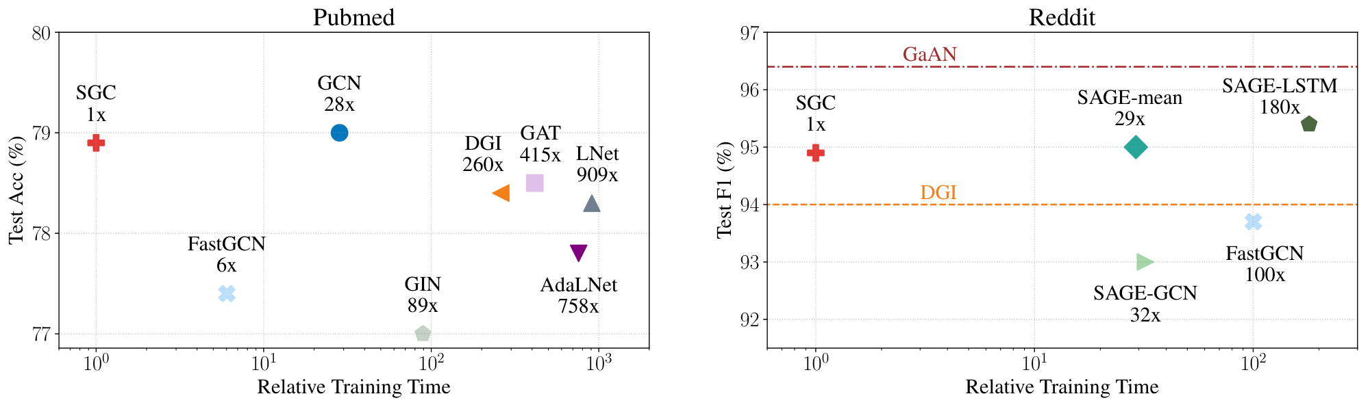
Efficiency.

In Figure 3, we plot the performance of the state-of-the-arts graph networks over their training time relative to that of SGC on the Pubmed and Reddit datasets. In particular, we precompute ${\mathbf{S}}^K {\mathbf{X}}$ and the training time of SGC takes into account this precomputation time. We measure the training time on a NVIDIA GTX 1080 Ti GPU and present the benchmark details in supplementary materials.

On large graphs (e.g. Reddit), GCN cannot be trained due to excessive memory requirements. Previous approaches tackle this limitation by either sampling to reduce neighborhood size [2, 21] or limiting their model sizes [42]. By applying a fixed filter and precomputing ${\mathbf{S}}^K {\mathbf{X}}$, SGC minimizes memory usage and only learns a single weight matrix during training. Since ${\mathbf{S}}$ is typically sparse and $K$ is usually small, we can exploit fast sparse-dense matrix multiplication to compute ${\mathbf{S}}^K {\mathbf{X}}$. Figure 3 shows that SGC can be trained up to two orders of magnitude faster than fast sampling-based methods while having little or no drop in performance.

5.2 Downstream Tasks

We extend our empirical evaluation to 5 downstream applications — text classification, semi-supervised user geolocation, relation extraction, zero-shot image classification, and graph classification — to study the applicability of SGC. We describe experimental setup in supplementary materials.

\begin{tabular}{l|l|cc}
\toprule
Dataset & Model & Test Acc. $\uparrow$ & Time (seconds) $\downarrow$ \\
\midrule
\multirow{2}{*}{20NG} & GCN & $87.9 \pm{0.2}$ & $1205.1 \pm{144.5}$ \\ & { SGC} & $88.5 \pm{0.1}$ & $19.06 \pm{0.15}$ \\
\midrule
\multirow{2}{*}{R8} & GCN & $97.0 \pm{0.2}$ & $129.6 \pm{9.9}$ \\ & { SGC} & $97.2 \pm{0.1}$ & $1.90 \pm{0.03}$ \\
\midrule
\multirow{2}{*}{R52} & GCN & $93.8 \pm{0.2}$ & $245.0 \pm{13.0}$ \\ & { SGC} & $94.0 \pm{0.2}$ & $3.01 \pm{0.01}$ \\
\midrule
\multirow{2}{*}{Ohsumed} & GCN & $68.2 \pm{0.4}$ & $252.4 \pm{14.7}$ \\ & { SGC} & $68.5 \pm{0.3}$ & $3.02 \pm{0.02}$ \\
\midrule
\multirow{2}{*}{MR} & GCN & $76.3 \pm{0.3}$ & $16.1 \pm{0.4}$ \\ & { SGC} & $75.9 \pm{0.3}$ & $4.00 \pm{0.04}$ \\
\bottomrule
\end{tabular}

Text classification

assigns labels to documents. [4] use a 2-layer GCN to achieve state-of-the-art results by creating a corpus-level graph which treats both documents and words as nodes in a graph. Word-word edge weights are pointwise mutual information (PMI) and word-document edge weights are normalized TF-IDF scores. Table 4 shows that an SGC ($K=2$) rivals their model on 5 benchmark datasets, while being up to $83.6\times$ faster.

\begin{tabular}{l|l|rrrr}
\toprule
Dataset & Model & Acc.@161 $\uparrow$ & Time $\downarrow$ \\
\midrule
\multirow{2}{*}{GEOTEXT} & GCN+H & $60.6 \pm 0.2$ & $153.0$ s\\
& { SGC} & $61.1 \pm 0.1$ & $5.6$ s\\
\midrule
\multirow{2}{*}{TWITTER-US} & GCN+H & $61.9 \pm 0.2$ & $9$ h $54$ m \\
& { SGC} & $62.5 \pm 0.1$ & $4$ h $33$ m \\
\midrule
\multirow{2}{*}{TWITTER-WORLD} & GCN+H & $53.6 \pm 0.2$ & $2$ d $05$ h $17$ m \\
& { SGC} & $54.1 \pm 0.2$ & $22$ h $53$ m \\
\bottomrule
\end{tabular}

Semi-supervised user geolocation

locates the "home" position of users on social media given users' posts, connections among users, and a small number of labelled users. [50] apply GCNs with highway connections on this task and achieve close to state-of-the-art results. Table 5 shows that SGC outperforms GCN with highway connections on GEOTEXT ([51]), TWITTER-US ([52]), and TWITTER-WORLD ([5]) under [50]'s framework, while saving $30+$ hours on TWITTER-WORLD.

:Table 6: Test Accuracy (%) on Relation Extraction. The numbers are averaged over 10 runs.

TACRED	Test Accuracy $\uparrow$
C-GCN ([6])	$66.4$
C-GCN	$66.4 \pm{0.4}$
C- SGC	$67.0 \pm{0.4}$

Relation extraction

involves predicting the relation between subject and object in a sentence. [6] propose C-GCN which uses an LSTM ([53]) followed by a GCN and an MLP. We replace GCN with SGC ($K=2$) and call the resulting model C-SGC. Table 6 shows that C-SGC sets new state-of-the-art on TACRED ([54]).

\begin{tabular}{l|l|l|l}
\toprule
Model & \# Param. $\downarrow$ & 2-hop Acc. $\uparrow$ & 3-hop Acc. $\uparrow$ \\
 \midrule
\multicolumn{4}{l}{\textbf{Unseen categories only:}} \\
EXEM 1-nns & - & $27.0$ & $7.1$ \\ 
ADGPM & - & $26.6$ & $6.3$ \\
GCNZ & - & $19.8$ & $4.1$ \\
GCNZ (ours) & $9.5M$ & $20.9 \pm 0.2$ & $4.3 \pm 0.0$ \\
{ MLP- SGCZ (ours)} & $4.3M$ & $21.2 \pm 0.2$ & $4.4 \pm 0.1$ \\
\midrule
\multicolumn{4}{l}{\textbf{Unseen categories \& seen categories:}} \\
ADGPM & - & $10.3$ & $2.9$ \\
GCNZ & - & $9.7$ & $2.2$ \\
GCNZ (ours) & $9.5M$ & $10.0 \pm 0.2$ & $2.4 \pm 0.0$ \\
{ MLP- SGCZ (ours)} & $4.3M$ & $10.5 \pm 0.1$ & $2.5 \pm 0.0$ \\
 \bottomrule
\end{tabular}

Zero-shot image classification

consists of learning an image classifier without access to any images or labels from the test categories. GCNZ ([7]) uses a GCN to map the category names — based on their relations in WordNet ([56]) — to image feature domain, and find the most similar category to a query image feature vector. Table 7 shows that replacing GCN with an MLP followed by SGC can improve performance while reducing the number of parameters by $55%$. We find that an MLP feature extractor is necessary in order to map the pretrained GloVe vectors to the space of visual features extracted by a ResNet-50. Again, this downstream application demonstrates that learned graph convolution filters are superfluous; similar to [55]'s observation that GCNs may not be necessary.

Graph classification

requires models to use graph structure to categorize graphs. [24] theoretically show that GCNs are not sufficient to distinguish certain graph structures and show that their GIN is more expressive and achieves state-of-the-art results on various graph classification datasets. We replace the GCN in DCGCN ([57]) with an SGC and get $71.0%$ and $76.2%$ on NCI1 and COLLAB datasets ([58]) respectively, which is on par with an GCN counterpart, but far behind GIN. Similarly, on QM8 quantum chemistry dataset ([59]), more advanced AdaLNet and LNet ([3]) get $0.01$ MAE on QM8, outperforming SGC's $0.03$ MAE by a large margin.

6. Conclusion

Section Summary: Researchers introduce SGC, a straightforward graph convolutional model that involves basic graph pre-processing followed by simple logistic regression, yet it matches or exceeds the performance of more complex models like GCNs on various tasks while training dramatically faster—for instance, up to 100 times quicker on large datasets. Their analysis views SGC as a low-pass filter that smooths features across graphs by focusing on low-frequency signals, revealing that GCNs' strength likely stems from repeated graph propagation rather than nonlinear transformations, and explaining enhancements like the renormalization trick. Overall, SGC offers clear benefits as an easy starting model for node classification, a strong baseline for comparisons, and a foundation for advancing graph learning research by building complexity from simplicity.

In order to better understand and explain the mechanisms of GCNs, we explore the simplest possible formulation of a graph convolutional model, SGC. The algorithm is almost trivial, a graph based pre-processing step followed by standard multi-class logistic regression. However, the performance of SGC rivals — if not surpasses — the performance of GCNs and state-of-the-art graph neural network models across a wide range of graph learning tasks. Moreover by precomputing the fixed feature extractor ${\mathbf{S}}^K$, training time is reduced to a record low. For example on the Reddit dataset, SGC can be trained up to two orders of magnitude faster than sampling-based GCN variants.

In addition to our empirical analysis, we analyze SGC from a convolution perspective and manifest this method as a low-pass-type filter on the spectral domain. Low-pass-type filters capture low-frequency signals, which corresponds with smoothing features across a graph in this setting. Our analysis also provides insight into the empirical boost of the ``renormalization trick" and demonstrates how shrinking the spectral domain leads to a low-pass-type filter which underpins SGC.

Ultimately, the strong performance of SGC sheds light onto GCNs. It is likely that the expressive power of GCNs originates primarily from the repeated graph propagation (which SGC preserves) rather than the nonlinear feature extraction (which it doesn't.)

Given its empirical performance, efficiency, and interpretability, we argue that the SGC should be highly beneficial to the community in at least three ways: (1) as a first model to try, especially for node classification tasks; (2) as a simple baseline for comparison with future graph learning models; (3) as a starting point for future research in graph learning — returning to the historic machine learning practice to develop complex from simple models.

Acknowledgement

Section Summary: This research received funding from various organizations, including multiple grants from the National Science Foundation, the Office of Naval Research, the Bill and Melinda Gates Foundation, and Facebook Research, along with support from SAP America Inc. One researcher, Amauri Holanda de Souza Jr., also acknowledges financial help from Brazil's National Council for Scientific and Technological Development. The team expresses gratitude for helpful discussions with colleagues Xiang Fu, Shengyuan Hu, Shangdi Yu, Wei-Lun Chao, and Geoff Pleiss, as well as assistance with figure designs from Boyi Li.

This research is supported in part by grants from the National Science Foundation (III-1618134, III-1526012, IIS1149882, IIS-1724282, and TRIPODS-1740822), the Office of Naval Research DOD (N00014-17-1-2175), Bill and Melinda Gates Foundation, and Facebook Research. We are thankful for generous support by SAP America Inc. Amauri Holanda de Souza Jr. thanks CNPq (Brazilian Council for Scientific and Technological Development) for the financial support. We appreciate the discussion with Xiang Fu, Shengyuan Hu, Shangdi Yu, Wei-Lun Chao and Geoff Pleiss as well as the figure design support from Boyi Li.

Appendix: Simplifying Graph Convolutional Networks (Supplementary Material)

Section Summary: This appendix explores the mathematical properties of a special matrix called the augmented normalized Laplacian, which is used in graph convolutional networks to process data on connected networks like social graphs. It proves that this matrix is always non-negative and symmetric, meaning it has no negative eigenvalues and treats inputs fairly, and that zero is its smallest eigenvalue, reflecting the graph's overall connectivity. Additionally, it establishes bounds on the matrix's other eigenvalues, linking them to the varying degrees of nodes in the graph, which helps simplify the design of these networks.

A. The spectrum of $\tilde{\boldsymbol{\Delta}}_{\text{sym}}$

The normalized Laplacian defined on graphs with self-loops, $\tilde{\boldsymbol{\Delta}}_{\text{sym}}$, consists of an instance of generalized graph Laplacians and hold the interpretation as a difference operator, i.e. for any signal ${\mathbf{x}} \in \mathbb{R}^n$ it satisfies

$ (\tilde{\boldsymbol{\Delta}}{\text{sym}} {\mathbf{x}})i = \sum{j} \frac{\tilde{a}{ij}}{\sqrt{d_i + \gamma}} \left(\frac{x_i}{\sqrt{d_i + \gamma}} - \frac{x_j}{\sqrt{d_j + \gamma}}\right). \nonumber $

Here, we prove several properties regarding its spectrum.

########## {type="Lemma"}

(Non-negativity of $\tilde{\boldsymbol{\Delta}}_{\text{sym}}$) The augmented normalized Laplacian matrix is symmetric positive semi-definite.

Proof: The quadratic form associated with $\tilde{\boldsymbol{\Delta}}_{\text{sym}}$ is

$ \begin{align} & {\mathbf{x}}^\top\tilde{\boldsymbol{\Delta}}{\text{sym}}{\mathbf{x}} = \sum_i x_i^2 - \sum_i \sum_j\frac{\tilde{a}{ij} x_i x_j}{\sqrt{(d_i + \gamma)(d_j + \gamma)}} \nonumber \ & = \frac{1}{2} \left(\sum_i x_i^2 + \sum_j x_j^2 - \sum_i \sum_j \frac{2\tilde{a}{ij} x_i x_j}{\sqrt{(d_i + \gamma)(d_j + \gamma)}}\right) \nonumber \ & = \frac{1}{2} \left(\sum_i \sum_j \frac{\tilde{a}{ij} x_i^2}{d_i + \gamma} + \sum_j \sum_i \frac{\tilde{a}{ij} x_j^2}{d_j + \gamma} \right. \nonumber \ & \left. \quad \quad - \sum_i \sum_j \frac{2\tilde{a}{ij} x_i x_j}{\sqrt{(d_i + \gamma)(d_j + \gamma)}}\right) \nonumber \ & = \frac{1}{2} \sum_i \sum_j \tilde{a}_{ij}\left(\frac{x_i}{\sqrt{d_i + \gamma}} - \frac{x_j}{\sqrt{d_j + \gamma}}\right)^2 \geq 0 \end{align}\tag{10} $

########## {caption="Lemma 2"}

$0$ is an eigenvalue of both $\boldsymbol{\Delta}{\text{sym}}$ and $\tilde{\boldsymbol{\Delta}}{\text{sym}}$.

Proof: First, note that ${\mathbf{v}}=[1, \ldots, 1]^\top$ is an eigenvector of $\boldsymbol{\Delta}$ associated with eigenvalue $0$, i.e., $\boldsymbol{\Delta} {\mathbf{v}} = ({\mathbf{D}}- {\mathbf{A}}){\mathbf{v}} = \mathbf{0}$.

Also, we have that $\tilde{\boldsymbol{\Delta}}_{\text{sym}} = \tilde{{\mathbf{D}}}^{-1/2}(\tilde{{\mathbf{D}}} - \tilde{{\mathbf{A}}})\tilde{{\mathbf{D}}}^{-1/2} = \tilde{{\mathbf{D}}}^{-1/2}\boldsymbol{\Delta}\tilde{{\mathbf{D}}}^{-1/2}$. Denote ${\mathbf{v}}_1=\tilde{{\mathbf{D}}}^{1/2}{\mathbf{v}}$, then

$ \tilde{\boldsymbol{\Delta}}_{\text{sym}}{\mathbf{v}}_1 = \tilde{{\mathbf{D}}}^{-1/2}\boldsymbol{\Delta}\tilde{{\mathbf{D}}}^{-1/2}\tilde{{\mathbf{D}}}^{1/2}{\mathbf{v}} = \tilde{{\mathbf{D}}}^{-1/2} \boldsymbol{\Delta} {\mathbf{v}} = \mathbf{0}. $

Therefore, ${\mathbf{v}}1=\tilde{{\mathbf{D}}}^{1/2}{\mathbf{v}}$ is an eigenvector of $\tilde{\boldsymbol{\Delta}}{\text{sym}}$ associated with eigenvalue $0$, which is then the smallest eigenvalue from the non-negativity of $\tilde{\boldsymbol{\Delta}}{\text{sym}}$. Likewise, 0 can be proved to be the smallest eigenvalues of $\boldsymbol{\Delta}{\text{sym}}$.

########## {caption="Lemma 3"}

Let $\beta_1 \leq \beta_2 \leq \dots \leq \beta_n$ denote eigenvalues of ${\mathbf{D}}^{-1/2}{\mathbf{A}} {\mathbf{D}}^{-1/2}$ and $\alpha_1 \leq \alpha_2 \leq \dots \leq \alpha_n$ be the eigenvalues of $\tilde{{\mathbf{D}}}^{-1/2}{\mathbf{A}}\tilde{{\mathbf{D}}}^{-1/2}$. Then,

$ \begin{align} & \alpha_1 \geq \frac{\max_i d_i}{\gamma+\max_i d_i}\beta_1, &\alpha_n \leq \frac{\min_i{d_i}}{\gamma + \min_i{d_i}}. \end{align}\tag{11} $

Proof: We have shown that 0 is an eigenvalue of $\boldsymbol{\Delta}{\text{sym}}$. Since ${\mathbf{D}}^{-1/2}{\mathbf{A}} {\mathbf{D}}^{-1/2} = {\mathbf{I}} - \boldsymbol{\Delta}{\text{sym}}$, then $1$ is an eigenvalue of ${\mathbf{D}}^{-1/2}{\mathbf{A}} {\mathbf{D}}^{-1/2}$. More specifically, $\beta_n = 1$. In addition, by combining the fact that $\operatorname{Tr}({\mathbf{D}}^{-1/2}{\mathbf{A}}{\mathbf{D}}^{-1/2})=0=\sum_i \beta_i$ with $\beta_n = 1$, we conclude that $\beta_1 < 0$.

By choosing ${\mathbf{x}}$ such that $\lVert {\mathbf{x}} \rVert =1$ and ${\mathbf{y}}= {\mathbf{D}}^{1/2}\tilde{{\mathbf{D}}}^{-1/2} {\mathbf{x}}$, we have that $| {\mathbf{y}}|^2=\sum\limits_i\frac{d_i}{d_i+\gamma}x_i^2$ and $\frac{\min_i d_i}{\gamma+\min_i d_i}\leq | {\mathbf{y}}|^2\leq \frac{\max_i d_i}{\gamma+\max_i d_i}$. Hence, we use the Rayleigh quotient to provide a lower bound to $\alpha_1$:

$ \begin{align*} \alpha_1 & = \min_{| {\mathbf{x}}|=1} \left({\mathbf{x}}^\top\tilde{{\mathbf{D}}}^{-1/2} {\mathbf{A}} \tilde{{\mathbf{D}}}^{-1/2} {\mathbf{x}} \right) \ & = \min_{| {\mathbf{x}}|=1} \left({\mathbf{y}}^\top {\mathbf{D}}^{-1/2} {\mathbf{A}} {\mathbf{D}}^{-1/2} {\mathbf{y}} \right) \text{(by replacing variable)} \ &= \min_{| {\mathbf{x}}|=1} \left(\frac{{\mathbf{y}}^\top {\mathbf{D}}^{-1/2} {\mathbf{A}} {\mathbf{D}}^{-1/2}{\mathbf{y}}}{| {\mathbf{y}}|^2}| {\mathbf{y}}|^2 \right) \ &\geq \min_{| {\mathbf{x}}|=1} \left(\frac{{\mathbf{y}}^\top {\mathbf{D}}^{-1/2} {\mathbf{A}} {\mathbf{D}}^{-1/2} {\mathbf{y}}}{| {\mathbf{y}}|^2} \right) \max_{| {\mathbf{x}}|=1} \left(| {\mathbf{y}}|^2 \right) \ & (\because \min (AB) \geq \min (A) \max(B) \text{ if } \min (A) < 0, \forall B > 0, \ &\text{ and \quad} \min_{| {\mathbf{x}}|=1} \left(\frac{{\mathbf{y}}^\top {\mathbf{D}}^{-1/2} {\mathbf{A}} {\mathbf{D}}^{-1/2} {\mathbf{y}}}{| {\mathbf{y}}|^2} \right) = \beta_1 < 0) \ &= \beta_1\max_{| {\mathbf{x}}|=1} | {\mathbf{y}}|^2 \ &\geq \frac{\max_i d_i}{\gamma+\max_i d_i}\beta_1.\ \end{align*} $

One may employ similar steps to prove the second inequality in Equation 11.

Proof of Theorem 1: Note that $\tilde{\boldsymbol{\Delta}}_{\text{sym}} = {\mathbf{I}} - \gamma \tilde{{\mathbf{D}}}^{-1} - \tilde{{\mathbf{D}}}^{-1/2}{\mathbf{A}}\tilde{{\mathbf{D}}}^{-1/2}$. Using the results in Lemma 3, we show that the largest eigenvalue $\tilde{\lambda}n$ of $\tilde{\boldsymbol{\Delta}}{\text{sym}}$ is

$ \begin{align} \tilde{\lambda}n & = \max{| {\mathbf{x}}|=1} {\mathbf{x}}^\top({\mathbf{I}} - \gamma \tilde{{\mathbf{D}}}^{-1} - \tilde{{\mathbf{D}}}^{-1/2}{\mathbf{A}}\tilde{{\mathbf{D}}}^{-1/2}){\mathbf{x}} \nonumber \ & \leq 1 - \min_{| {\mathbf{x}}|=1} \gamma {\mathbf{x}}^\top \tilde{{\mathbf{D}}}^{-1} {\mathbf{x}} - \min_{| {\mathbf{x}}|=1} {\mathbf{x}}^\top \tilde{{\mathbf{D}}}^{-1/2} {\mathbf{A}} \tilde{{\mathbf{D}}}^{-1/2} {\mathbf{x}} \nonumber \ & = 1 - \frac{\gamma}{\gamma + \max_{i} d_i} - \alpha_1 \nonumber \ & \leq 1 - \frac{\gamma}{\gamma + \max_{i} d_i} - \frac{\max_i d_i}{\gamma + \max_i d_i} \beta_1 \nonumber \ & < 1 - \frac{\max_i d_i}{\gamma + \max_i d_i} \beta_1 \quad (\gamma > 0 \text{ and } \beta_1 < 0) \nonumber \ & < 1 - \beta_1 = \lambda_n \end{align}\tag{12} $

B. Experiment Details

Node Classification.

We empirically find that on Reddit dataset for SGC, it is crucial to normalize the features into zero mean and univariate.

Training Time Benchmarking.

We hereby describe the experiment setup of Figure 3. [2] benchmark the training time of FastGCN on CPU, and as a result, it is difficult to compare numerical values across reports. Moreover, we found the performance of FastGCN improved with a smaller early stopping window (10 epochs); therefore, we could decrease the model's training time. We provide the data underpinning Figure 3 in Table 8 and Table 9.

:Table 8: Training time (seconds) of graph neural networks on Citation Networks. Numbers are averaged over 10 runs.

Models	Cora	Citeseer	Pubmed
GCN	$0.49$	$0.59$	$8.31$
GAT	$63.10$	$118.10$	$121.74$
FastGCN	$2.47$	$3.96 $	$1.77$
GIN	$2.09$	$4.47$	$26.15$
LNet	$15.02$	$49.16$	$266.47$
AdaLNet	$10.15$	$31.80$	$222.21$
DGI	$21.24$	$21.06$	$76.20$
SGC	$0.13$	$0.14$	$0.29$

:Table 9: Training time (seconds) on Reddit dataset.

Model	Time(s) $\downarrow$
SAGE-mean	$78.54$
SAGE-LSTM	$486.53$
SAGE-GCN	$86.86$
FastGCN	$270.45$
SGC	$2.70$

Text Classification.

[4] use one-hot features for the word and document nodes. In training SGC, we normalize the features to be between 0 and 1 after propagation and train with L-BFGS for 3 steps. We tune the only hyperparameter, weight decay, using hyperopt [48] for 60 iterations. Note that we cannot apply this feature normalization for TextGCN because the propagation cannot be precomputed.

Semi-supervised User Geolocation.

We replace the 4-layer, highway-connection GCN with a 3rd degree propagation matrix ($K=3$) SGC and use the same set of hyperparameters as [50]. All experiments on the GEOTEXT dataset are conducted on a single Nvidia GTX-1080Ti GPU while the ones on the TWITTER-NA and TWITTER-WORLD datasets are excuded with 10 cores of the Intel(R) Xeon(R) Silver 4114 CPU (2.20GHz). Instead of collapsing all linear transformations, we keep two of them which we find performing slightly better possibly due to . Despite of this subtle variation, the model is still linear.

Relation Extraction.

We replace the 2-layer GCN with a 2nd degree propagation matrix ($K=2$) SGC and remove the intermediate dropout. We keep other hyperparameters unchanged, including learning rate and regularization. Similar to [6], we report the best validation accuracy with early stopping.

Zero-shot Image Classification.

We replace the 6-layer GCN (hidden size: 2048, 2048, 1024, 1024, 512, 2048) baseline with an 6-layer MLP (hidden size: 512, 512, 512, 1024, 1024, 2048) followed by a SGC with $K=6$. Following [7], we only apply dropout to the output of SGC. Due to the slow evaluation of this task, we do not tune the dropout rate or other hyperparameters. Rather, we follow the GCNZ code and use learning rate of 0.001, weight decay of 0.0005, and dropout rate of 0.5. We also train the models with ADAM [47] for 300 epochs.

C. Additional Experiments

Random Splits for Citation Networks.

Possibly due to their limited size, the citation networks are known to be unstable. Accordingly, we conduct an additional 10 experiments on random splits of the training set while maintaining the same validation and test sets.

\begin{tabular}{l|c|c|c}
\toprule
 & Cora & Citeseer & Pubmed \\ 
\midrule
\multicolumn{4}{l}{\textbf{Ours:}} \\
GCN & $80.53 \pm{1.40}$ & $70.67\pm{2.90}$ & $77.09 \pm{2.95}$ \\
GIN & $76.94 \pm 1.24$ & $66.56 \pm 2.27$ & $74.46 \pm 2.19$ \\
LNet & $74.23 \pm 4.50^\dagger$ & $67.26 \pm 0.81^\dagger$ & $77.20 \pm 2.03^\dagger$ \\
AdaLNet & $72.68 \pm 1.45^\dagger$ & $71.04 \pm 0.95^\dagger$ & $77.53 \pm 1.76^\dagger$ \\
GAT & $82.29 \pm{1.16}$ & $72.6 \pm{0.58}$ & $78.79 \pm{1.41}$ \\
{ SGC} & $80.62 \pm{1.21}$ & $71.40 \pm{3.92}$ & $77.02 \pm{1.62} $ \\
 \bottomrule
\end{tabular}

Propagation choice.

We conduct an ablation study with different choices of propagation matrix, namely:

• Normalized Adjacency: $\mathbf{S}_{\text{adj}} = {\mathbf{D}}^{-1/2}{\mathbf{A}} {\mathbf{D}}^{-1/2}$
• Random Walk Adjacency $\mathbf{S}_{\text{rw}} = {\mathbf{D}}^{-1}{\mathbf{A}}$
• Aug. Normalized Adjacency $\tilde{\mathbf{S}}_{\text{adj}} = \tilde{{\mathbf{D}}}^{-1/2}\tilde{{\mathbf{A}}} \tilde{{\mathbf{D}}}^{-1/2}$
• Aug. Random Walk $\tilde{\mathbf{S}}_{\text{rw}} = \tilde{{\mathbf{D}}}^{-1} \tilde{{\mathbf{A}}}$
• First-Order Cheby $\mathbf{S}_{\text{1-order}}=({\mathbf{I}} + {\mathbf{D}}^{-1/2}{\mathbf{A}} {\mathbf{D}}^{-1/2})$

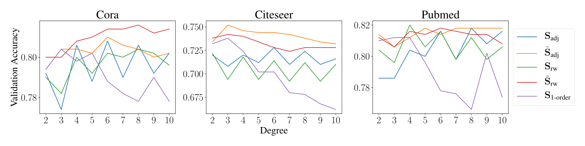
We investigate the effect of propagation steps $K \in {2..10}$ on validation set accuracy. We use hyperopt to tune L2-regularization and leave all other hyperparameters unchanged. Figure 4 depicts the validation results achieved by varying the degree of different propagation matrices.

We see that augmented propagation matrices (i.e. those with self-loops) attain higher accuracy and more stable performance across various propagation depths. Specifically, the accuracy of $\mathbf{S}_{\text{1-order}}$ tends to deteriorate as the power $K$ increases, and this results suggests using large filter coefficients on low frequencies degrades SGC performance on semi-supervised tasks.

Another pattern is that odd powers of $K$ cause a significant performance drop for the normalized adjacency and random walk propagation matrices. This demonstrates how odd powers of the un-augmented propagation matrix use negative filter coefficients on high frequency information. Adding self-loops to the propagation matrix shrinks the spectrum such that the largest eigenvalues decrease from $\approx 2$ to $\approx 1.5$ on the citation network datasets. By effectively shrinking the spectrum, the effect of negative filter coefficients on high frequencies is minimized, and as a result, using odd-powers of $K$ does not degrade the performance of augmented propagation matrices. For non-augmented propagation matrices — where the largest eigenvalue is approximately 2 — negative coefficients significantly distort the signal, which leads to decreased accuracy. Therefore, adding self-loops constructs a better domain in which fixed filters can operate.

:Table 11: Validation Accuracy (%) when SGC and GCN are trained with different amounts of data on Cora. The validation accuracy is averaged over 10 random training splits such that each class has the same number of training examples.

# Training Samples	SGC	GCN
1	33.16	32.94
5	63.74	60.68
10	72.04	71.46
20	80.30	80.16
40	85.56	85.38
80	90.08	90.44

Data amount.

We also investigated the effect of training dataset size on accuracy. As demonstrated in Table 11, SGC continues to perform similarly to GCN as the training dataset size is reduced, and even outperforms GCN when there are fewer than $5$ training samples. We reason this study demonstrates SGC has at least the same modeling capacity as GCN.

References

[1] Kipf, T. N. and Welling, M. Semi-supervised classification with graph convolutional networks. In International Conference on Learning Representations (ICLR'2017), 2017.

[2] Chen, J., Ma, T., and Xiao, C. FastGCN: Fast Learning with Graph Convolutional Networks via Importance Sampling. In International Conference on Learning Representations (ICLR'2018), 2018.

[3] Liao, R., Zhao, Z., Urtasun, R., and Zemel, R. Lanczosnet: Multi-scale deep graph convolutional networks. In International Conference on Learning Representations (ICLR'2019), 2019.

[4] Yao, L., Mao, C., and Luo, Y. Graph convolutional networks for text classification. In Proceedings of the 33rd AAAI Conference on Artificial Intelligence (AAAI'19), 2019.

[5] Han, B., Cook, P., and Baldwin, T. Geolocation prediction in social media data by finding location indicative words. In Proceedings of the 24th International Conference on Computational Linguistics, pp.\ 1045–1062, 2012.

[6] Zhang, Y., Qi, P., and Manning, C. D. Graph convolution over pruned dependency trees improves relation extraction. In Empirical Methods in Natural Language Processing (EMNLP), 2018c.

[7] Wang, X., Ye, Y., and Gupta, A. Zero-shot recognition via semantic embeddings and knowledge graphs. In Computer Vision and Pattern Recognition (CVPR), pp.\ 6857–6866. IEEE Computer Society, 2018.

[8] Kampffmeyer, M., Chen, Y., Liang, X., Wang, H., Zhang, Y., and Xing, E. P. Rethinking knowledge graph propagation for zero-shot learning. arXiv preprint arXiv:1805.11724, 2018.

[9] Rosenblatt, F. The Perceptron: a probabilistic model for information storage and organization in the brain. Psychological review, 65(6):386, 1958.

[10] Rosenblatt, F. Principles of neurodynamics: Perceptrons and the theory of brain mechanisms. Technical report, Cornell Aeronautical Lab Inc, 1961.

[11] Sobel, I. and Feldman, G. A 3x3 isotropic gradient operator for image processing. A talk at the Stanford Artificial Project, pp.\ 271–272, 1968.

[12] Harris, C. and Stephens, M. A combined corner and edge detector. In Proceedings of the 4th Alvey Vision Conference, pp.\ 147–151, 1988.

[13] Waibel, A., Hanazawa, T., and Hinton, G. Phoneme recognition using time-delay neural networks. IEEE Transactions on Acoustics, Speech. and Signal Processing, 37(3), 1989.

[14] LeCun, Y., Boser, B., Denker, J. S., Henderson, D., Howard, R. E., Hubbard, W., and Jackel, L. D. Backpropagation applied to handwritten zip code recognition. Neural Computation, 1(4):541–551, 1989.

[15] Bruna, J., Zaremba, W., Szlam, A., and Lecun, Y. Spectral networks and locally connected networks on graphs. In International Conference on Learning Representations (ICLR'2014), 2014.

[16] Hariharan, B., Arbeláez, P., Girshick, R., and Malik, J. Hypercolumns for object segmentation and fine-grained localization. In Proceedings of the IEEE conference on computer vision and pattern recognition, pp.\ 447–456, 2015.

[17] Huang, G., Sun, Y., Liu, Z., Sedra, D., and Weinberger, K. Q. Deep networks with stochastic depth. In European Conference on Computer Vision, pp.\ 646–661. Springer, 2016.

[18] Bottou, L. Large-scale machine learning with stochastic gradient descent. In Proceedings of 19th International Conference on Computational Statistics, pp.\ 177–186. Springer, 2010.

[19] Sen, P., Namata, G., Bilgic, M., Getoor, L., Galligher, B., and Eliassi-Rad, T. Collective classification in network data. AI magazine, 29(3):93, 2008.

[20] Defferrard, M., Bresson, X., and Vandergheynst, P. Convolutional neural networks on graphs with fast localized spectral filtering. In Lee, D. D., Sugiyama, M., Luxburg, U. V., Guyon, I., and Garnett, R. (eds.), Advances in Neural Information Processing Systems 29, pp.\ 3844–3852. Curran Associates, Inc., 2016.

[21] Hamilton, W., Ying, Z., and Leskovec, J. Inductive representation learning on large graphs. In Guyon, I., Luxburg, U. V., Bengio, S., Wallach, H., Fergus, R., Vishwanathan, S., and Garnett, R. (eds.), Advances in Neural Information Processing Systems 30, pp.\ 1024–1034. Curran Associates, Inc., 2017.

[22] Atwood, J. and Towsley, D. Diffusion-convolutional neural networks. In Lee, D. D., Sugiyama, M., Luxburg, U. V., Guyon, I., and Garnett, R. (eds.), Advances in Neural Information Processing Systems 29, pp.\ 1993–2001. Curran Associates, Inc., 2016.

[23] Abu-El-Haija, S., Kapoor, A., Perozzi, B., and Lee, J. N-GCN: Multi-scale graph convolution for semi-supervised node classification. arXiv preprint arXiv:1802.08888, 2018.

[24] Xu, K., Hu, W., Leskovec, J., and Jegelka, S. How powerful are graph neural networks? In International Conference on Learning Representations (ICLR'2019), 2019.

[25] Klicpera, J., Bojchevski, A., and Günnemann, S. Predict then propagate: Graph neural networks meet personalized pagerank. In International Conference on Learning Representations (ICLR'2019), 2019.

[26] Monti, F., Boscaini, D., Masci, J., Rodolà, E., Svoboda, J., and Bronstein, M. M. Geometric deep learning on graphs and manifolds using mixture model cnns. In 2017 IEEE Conference on Computer Vision and Pattern Recognition, CVPR 2017, Honolulu, HI, USA, July 21-26, 2017, pp.\ 5425–5434, 2017.

[27] Duran, A. G. and Niepert, M. Learning graph representations with embedding propagation. In Guyon, I., Luxburg, U. V., Bengio, S., Wallach, H., Fergus, R., Vishwanathan, S., and Garnett, R. (eds.), Advances in Neural Information Processing Systems 30, pp.\ 5119–5130. Curran Associates, Inc., 2017.

[28] Li, Q., Han, Z., and Wu, X. Deeper insights into graph convolutional networks for semi-supervised learning. CoRR, abs/1801.07606, 2018.

[29] Zhou, J., Cui, G., Zhang, Z., Yang, C., Liu, Z., and Sun, M. Graph Neural Networks: A Review of Methods and Applications. arXiv e-prints, 2018.

[30] Battaglia, P. W., Hamrick, J. B., Bapst, V., Sanchez-Gonzalez, A., Zambaldi, V., Malinowski, M., Tacchetti, A., Raposo, D., Santoro, A., Faulkner, R., et al. Relational inductive biases, deep learning, and graph networks. arXiv preprint arXiv:1806.01261, 2018.

[31] Wu, Z., Pan, S., Chen, F., Long, G., Zhang, C., and Yu, P. S. A comprehensive survey on graph neural networks. arXiv preprint arXiv:1901.00596, 2019.

[32] Thekumparampil, K. K., Wang, C., Oh, S., and Li, L. Attention-based graph neural network for semi-supervised learning. arXiv e-prints, 2018.

[33] Cai, C. and Wang, Y. A simple yet effective baseline for non-attribute graph classification, 2018.

[34] Eliav, B. and Cohen, E. Bootstrapped graph diffusions: Exposing the power of nonlinearity. Proceedings of the ACM on Measurement and Analysis of Computing Systems, 2(1):10:1–10:19, 2018.

[35] Li, Q., Wu, X.-M., Liu, H., Zhang, X., and Guan, Z. Label efficient semi-supervised learning via graph filtering. In IEEE/CVF Conference on Computer Vision and Pattern Recognition (CVPR), 2019.

[36] Velickovic, P., Cucurull, G., Casanova, A., Romero, A., Liò, P., and Bengio, Y. Graph Attention Networks. In International Conference on Learning Representations (ICLR'2018), 2018.

[37] Zhang, J., Shi, X., Xie, J., Ma, H., King, I., and Yeung, D. Gaan: Gated attention networks for learning on large and spatiotemporal graphs. In Proceedings of the Thirty-Fourth Conference on Uncertainty in Artificial Intelligence (UAI'2018), pp.\ 339–349. AUAI Press, 2018a.

[38] Lee, J. B., Rossi, R. A., Kim, S., Ahmed, N. K., and Koh, E. Attention models in graphs: A survey. arXiv e-prints, 2018.

[39] Weston, J., Ratle, F., and Collobert, R. Deep learning via semi-supervised embedding. In Proceedings of the 25th International Conference on Machine Learning, ICML '08, pp.\ 1168–1175, 2008.

[40] Perozzi, B., Al-Rfou, R., and Skiena, S. Deepwalk: Online learning of social representations. In Proceedings of the 20th ACM SIGKDD International Conference on Knowledge Discovery and Data Mining, KDD'14, pp.\ 701–710. ACM, 2014.

[41] Yang, Z., Cohen, W. W., and Salakhutdinov, R. Revisiting semi-supervised learning with graph embeddings. In Proceedings of the 33rd International Conference on International Conference on Machine Learning - Volume 48, ICML'16, pp.\ 40–48, 2016.

[42] Veličković, P., Fedus, W., Hamilton, W. L., Liò, P., Bengio, Y., and Hjelm, R. D. Deep Graph InfoMax. In International Conference on Learning Representations (ICLR'2019), 2019.

[43] Zhu, X., Ghahramani, Z., and Lafferty, J. Semi-supervised learning using gaussian fields and harmonic functions. In Proceedings of the Twentieth International Conference on International Conference on Machine Learning, ICML'03, pp.\ 912–919. AAAI Press, 2003.

[44] Zhou, D., Bousquet, O., Thomas, N. L., Weston, J., and Schölkopf, B. Learning with local and global consistency. In Thrun, S., Saul, L. K., and Schölkopf, B. (eds.), Advances in Neural Information Processing Systems 16, pp.\ 321–328. MIT Press, 2004.

[45] Belkin, M. and Niyogi, P. Semi-supervised learning on riemannian manifolds. Machine Learning, 56(1-3):209–239, 2004.

[46] Belkin, M., Niyogi, P., and Sindhwani, V. Manifold regularization: A geometric framework for learning from labeled and unlabeled examples. Journal of Machine Learning Research, 7:2399–2434, 2006.

[47] Kingma, D. P. and Ba, J. Adam: A method for stochastic optimization. In International Conference on Learning Representations (ICLR'2015), 2015.

[48] Bergstra, J., Komer, B., Eliasmith, C., Yamins, D., and Cox, D. D. Hyperopt: A python library for optimizing the hyperparameters of machine learning algorithms. Computational Science & Discovery, 8(1), 2015.

[49] Liu, D. C. and Nocedal, J. On the limited memory BFGS method for large scale optimization. Mathematical Programming, 45(1-3):503–528, 1989.

[50] Rahimi, S., Cohn, T., and Baldwin, T. Semi-supervised user geolocation via graph convolutional networks. In Proceedings of the 56th Annual Meeting of the Association for Computational Linguistics (Volume 1: Long Papers), pp.\ 2009–2019. Association for Computational Linguistics, 2018.

[51] Eisenstein, J., O'Connor, B., Smith, N. A., and Xing, E. P. A latent variable model for geographic lexical variation. In Proceedings of the 2010 Conference on Empirical Methods in Natural Language Processing, pp.\ 1277–1287. Association for Computational Linguistics, 2010.

[52] Roller, S., Speriosu, M., Rallapalli, S., Wing, B., and Baldridge, J. Supervised text-based geolocation using language models on an adaptive grid. In Proceedings of the 2012 Joint Conference on Empirical Methods in Natural Language Processing and Computational Natural Language Learning, pp.\ 1500–1510. Association for Computational Linguistics, 2012.

[53] Hochreiter, S. and Schmidhuber, J. Long Short-Term Memory. Neural Computation, 9:1735–1780, 1997.

[54] Zhang, Y., Zhong, V., Chen, D., Angeli, G., and Manning, C. D. Position-aware attention and supervised data improve slot filling. In Proceedings of the 2017 Conference on Empirical Methods in Natural Language Processing, pp.\ 35–45. Association for Computational Linguistics, 2017.

[55] Changpinyo, S., Chao, W.-L., Gong, B., and Sha, F. Classifier and exemplar synthesis for zero-shot learning. arXiv preprint arXiv:1812.06423, 2018.

[56] Miller, G. A. Wordnet: a lexical database for english. Communications of the ACM, 38(11):39–41, 1995.

[57] Zhang, M., Cui, Z., Neumann, M., and Chen, Y. An end-to-end deep learning architecture for graph classification. 2018b.

[58] Yanardag, P. and Vishwanathan, S. Deep graph kernels. In Proceedings of the 21th ACM SIGKDD International Conference on Knowledge Discovery and Data Mining, pp.\ 1365–1374. ACM, 2015.

[59] Ramakrishnan, R., Hartmann, M., Tapavicza, E., and von Lilienfeld, O. A. Electronic spectra from TDDFT and machine learning in chemical space. The Journal of chemical physics, 143(8):084111, 2015.