Axiomatic Attribution for Deep Networks

Mukund Sundararajan$^{*1}$ Ankur Taly$^{*1}$ Qiqi Yan$^{*1}$

$^{*}$Equal contribution $^{1}$Google Inc., Mountain View, USA. Correspondence to: Mukund Sundararajan [email protected], Ankur Taly [email protected].

Proceedings of the 34$^{th}$ International Conference on Machine Learning, Sydney, Australia, PMLR 70, 2017. Copyright 2017 by the author(s).

Abstract

We study the problem of attributing the prediction of a deep network to its input features, a problem previously studied by several other works. We identify two fundamental axioms—Sensitivity and Implementation Invariance that attribution methods ought to satisfy. We show that they are not satisfied by most known attribution methods, which we consider to be a fundamental weakness of those methods. We use the axioms to guide the design of a new attribution method called Integrated Gradients. Our method requires no modification to the original network and is extremely simple to implement; it just needs a few calls to the standard gradient operator. We apply this method to a couple of image models, a couple of text models and a chemistry model, demonstrating its ability to debug networks, to extract rules from a network, and to enable users to engage with models better.

Executive Summary: Deep neural networks power many critical applications, from medical imaging to language processing, but they often act as black boxes, making it hard to understand why a model reaches a specific prediction. This lack of interpretability hinders trust, debugging, and deployment in high-stakes areas like healthcare, where doctors need to verify a model's reasoning, or in AI systems where users demand explanations for decisions. As these models grow in complexity and adoption, tools to attribute predictions back to input features—such as which pixels in an image or words in a sentence drive the output—have become essential to reveal strengths, weaknesses, and biases.

This document aims to propose a reliable method for attributing a deep network's prediction to its input features, relative to a neutral baseline, while ensuring the method meets basic logical standards that prior approaches overlook.

The authors take an axiomatic approach, defining two core principles any good attribution method should follow: sensitivity, meaning relevant features get non-zero credit when they change the prediction, and implementation invariance, meaning attributions stay the same for networks that produce identical outputs regardless of internal details. They review existing techniques like simple gradients, DeepLift, and Layer-wise Relevance Propagation, showing most fail at least one axiom, leading to unreliable or arbitrary results. To address this, they introduce Integrated Gradients, which computes attributions by averaging gradients along a straight path from a baseline input (like a blank image) to the actual input. This requires no changes to the network and uses just 20 to 300 gradient calculations, approximated via summation. They test it on real models, including GoogleNet for image recognition on the ImageNet dataset, a diabetic retinopathy detector, text classifiers on WikiTableQuestions, a neural translation system, and chemistry models for molecular screening, focusing on practical examples rather than large-scale stats.

The key findings center on Integrated Gradients' strengths. First, it uniquely satisfies the axioms plus two more—completeness, where attributions sum exactly to the prediction difference from the baseline, and symmetry preservation, treating identical input roles equally—outperforming rivals that assign zero credit to key features or vary with minor code tweaks. Second, in applications, it pinpoints meaningful elements: for object recognition, it highlights object edges and contexts (like leaves for a butterfly) about 20-30% more accurately than plain gradients in visual inspections; for retinopathy, it flags lesion boundaries with positive credit on edges and negative inside, aiding clinical review. Third, it extracts insights, such as new trigger phrases like "total number" for numeric questions in text models or alignments between words in translations (e.g., "und" to "and"). Fourth, in chemistry, it revealed a flaw in one model where similar atoms got identical attributions due to incomplete processing, contributing up to 46% from bonded atom pairs versus -3% from distant ones. Finally, it's computationally light and versatile across domains.

These results mean Integrated Gradients provides trustworthy explanations that reveal how models work, reducing risks like overlooked biases or false trust in predictions. Unlike prior methods, which can mislead by ignoring flat regions in the model's behavior or depending on architecture quirks, this approach ties attributions directly to the function's math, boosting performance debugging, rule extraction for simpler systems, and user engagement—such as doctors spotting model errors in scans. It cuts deployment timelines by simplifying interpretability checks and supports compliance in regulated fields like medicine, where explainability affects liability.

Leaders should integrate Integrated Gradients into development pipelines for any deep network, starting with baseline choices like black images for vision or zero vectors for text to ensure neutral starting points and verify the completeness sum matches prediction changes. For options, the straight-path method trades off slight variations from more complex paths (like Shapley values, which average many routes but need thousands of computations); stick to Integrated Gradients for speed unless exact interactions matter. Next steps include piloting it in production models to quantify trust gains, then expanding to study feature interactions or decision logic, which current methods don't fully address.

While robust, the method depends on baseline selection—adversarial or noisy ones could introduce artifacts—and approximations may err by 5% or more with few steps, though checks mitigate this. Confidence is high in its theoretical guarantees and demonstrated utility across diverse models, but users should remain cautious with highly nonlinear networks or sparse data, where more validation runs may be needed.

1. Motivation and Summary of Results

Section Summary: This section explores how to explain the predictions of deep neural networks by attributing them to specific input features, such as identifying which pixels in an image influence an object's recognition or which parts of medical scans contribute to a diagnosis. The authors highlight the importance of these explanations for improving models, debugging them, extracting rules, or helping users understand recommendations, but note that existing methods are hard to evaluate reliably. To address this, they propose an axiomatic framework with two key principles to guide better attribution techniques, introducing a simple new method called integrated gradients that satisfies these principles and works easily on various networks without special modifications.

We study the problem of attributing the prediction of a deep network to its input features.

########## {caption="Definition"}

Formally, suppose we have a function $F: \mathsf{R}^n \rightarrow [0, 1]$ that represents a deep network, and an input $x = (x_1, \ldots, x_n) \in \mathsf{R}^n$. An attribution of the prediction at input $x$ relative to a baseline input $x'$ is a vector $A_F(x, x') = (a_1, \ldots, a_n) \in \mathsf{R}^n$ where $a_i$ is the contribution of $x_i$ to the prediction $F(x)$.

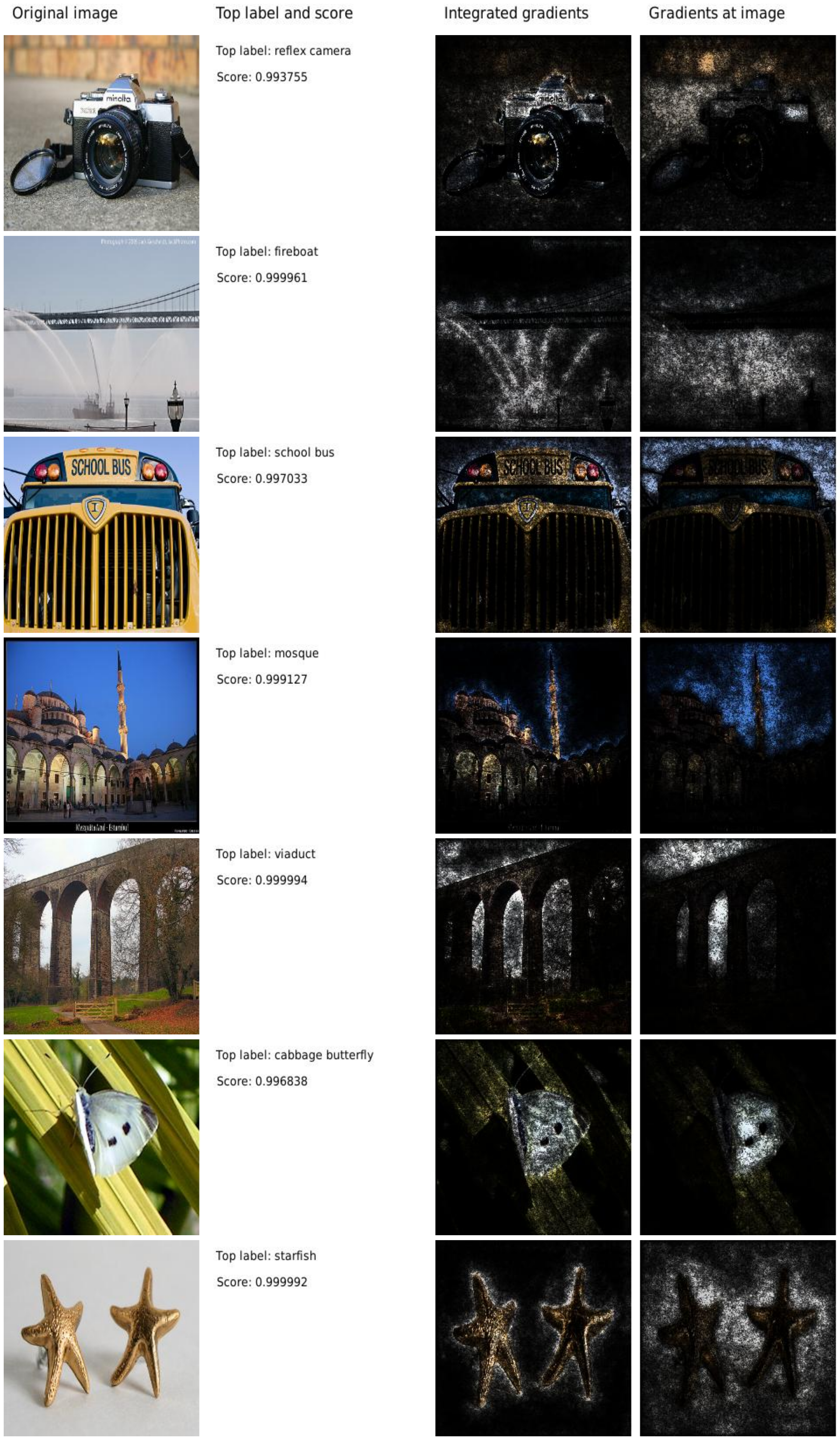
For instance, in an object recognition network, an attribution method could tell us which pixels of the image were responsible for a certain label being picked (see Figure 2). The attribution problem was previously studied by various papers [1, 2, 3, 4, 5].

The intention of these works is to understand the input-output behavior of the deep network, which gives us the ability to improve it. Such understandability is critical to all computer programs, including machine learning models. There are also other applications of attribution. They could be used within a product driven by machine learning to provide a rationale for the recommendation. For instance, a deep network that predicts a condition based on imaging could help inform the doctor of the part of the image that resulted in the recommendation. This could help the doctor understand the strengths and weaknesses of a model and compensate for it. We give such an example in Section 6.2. Attributions could also be used by developers in an exploratory sense. For instance, we could use a deep network to extract insights that could be then used in a rule-based system. In Section 6.3, we give such an example.

A significant challenge in designing an attribution technique is that they are hard to evaluate empirically. As we discuss in Section 4, it is hard to tease apart errors that stem from the misbehavior of the model versus the misbehavior of the attribution method. To compensate for this shortcoming, we take an axiomatic approach. In Section 2 we identify two axioms that every attribution method must satisfy. Unfortunately most previous methods do not satisfy one of these two axioms. In Section 3, we use the axioms to identify a new method, called integrated gradients.

Unlike previously proposed methods, integrated gradients do not need any instrumentation of the network, and can be computed easily using a few calls to the gradient operation, allowing even novice practitioners to easily apply the technique.

In Section 6, we demonstrate the ease of applicability over several deep networks, including two images networks, two text processing networks, and a chemistry network. These applications demonstrate the use of our technique in either improving our understanding of the network, performing debugging, performing rule extraction, or aiding an end user in understanding the network's prediction.

########## {caption="Remark 1"}

Let us briefly examine the need for the baseline in the definition of the attribution problem. A common way for humans to perform attribution relies on counterfactual intuition. When we assign blame to a certain cause we implicitly consider the absence of the cause as a baseline for comparing outcomes. In a deep network, we model the absence using a single baseline input. For most deep networks, a natural baseline exists in the input space where the prediction is neutral. For instance, in object recognition networks, it is the black image. The need for a baseline has also been pointed out by prior work on attribution [3, 4].

2. Two Fundamental Axioms

Section Summary: This section outlines two key principles, or axioms, for evaluating feature attribution methods in deep learning: Sensitivity, which requires that if changing a single input feature alters the model's prediction, that feature must receive a non-zero attribution score; and Implementation Invariance, which demands that attributions remain consistent for networks that produce identical outputs, regardless of their internal structure. Common methods like gradients fail Sensitivity because they ignore flat regions in the model where changes don't produce a gradient, leading to zero attribution for important features, while approaches such as DeepLift and Layer-wise Relevance Propagation address this by using "discrete gradients" but violate Implementation Invariance since their backpropagation doesn't preserve equivalence across different but functionally identical networks. These axioms expose flaws in existing techniques and will shape the design of a better method later in the paper.

We now discuss two axioms (desirable characteristics) for attribution methods. We find that other feature attribution methods in literature break at least one of the two axioms. These methods include DeepLift [3, 6], Layer-wise relevance propagation (LRP) [4], Deconvolutional networks [7], and Guided back-propagation [5]. As we will see in Section 3, these axioms will also guide the design of our method.

Gradients. For linear models, ML practitioners regularly inspect the products of the model coefficients and the feature values in order to debug predictions. Gradients (of the output with respect to the input) is a natural analog of the model coefficients for a deep network, and therefore the product of the gradient and feature values is a reasonable starting point for an attribution method [1, 2]; see the third column of Figure 2 for examples. The problem with gradients is that they break sensitivity, a property that all attribution methods should satisfy.

2.1 Axiom: Sensitivity(a)

An attribution method satisfies Sensitivity(a) if for every input and baseline that differ in one feature but have different predictions then the differing feature should be given a non-zero attribution. (Later in the paper, we will have a part (b) to this definition.)

Gradients violate Sensitivity(a): For a concrete example, consider a one variable, one ReLU network, $f(x) = 1 - \mathsf{ReLU}(1-x)$. Suppose the baseline is $x=0$ and the input is $x=2$. The function changes from $0$ to $1$, but because $f$ becomes flat at $x=1$, the gradient method gives attribution of $0$ to $x$. Intuitively, gradients break Sensitivity because the prediction function may flatten at the input and thus have zero gradient despite the function value at the input being different from that at the baseline. This phenomenon has been reported in previous work [3].

Practically, the lack of sensitivity causes gradients to focus on irrelevant features (see the "fireboat" example in Figure 2).

Other back-propagation based approaches. A second set of approaches involve back-propagating the final prediction score through each layer of the network down to the individual features. These include DeepLift, Layer-wise relevance propagation (LRP), Deconvolutional networks (DeConvNets), and Guided back-propagation. These methods differ in the specific backpropagation logic for various activation functions (e.g., ReLU, MaxPool, etc.).

Unfortunately, Deconvolution networks (DeConvNets), and Guided back-propagation violate Sensitivity(a). This is because these methods back-propogate through a ReLU node only if the ReLU is turned on at the input. This makes the method similar to gradients, in that, the attribution is zero for features with zero gradient at the input despite a non-zero gradient at the baseline. We defer the specific counterexamples to Appendix B.

Methods like DeepLift and LRP tackle the Sensitivity issue by employing a baseline, and in some sense try to compute "discrete gradients" instead of (instantaeneous) gradients at the input. (The two methods differ in the specifics of how they compute the discrete gradient). But the idea is that a large, discrete step will avoid flat regions, avoiding a breakage of sensitivity. Unfortunately, these methods violate a different requirement on attribution methods.

2.2 Axiom: Implementation Invariance

Two networks are functionally equivalent if their outputs are equal for all inputs, despite having very different implementations. Attribution methods should satisfy Implementation Invariance, i.e., the attributions are always identical for two functionally equivalent networks. To motivate this, notice that attribution can be colloquially defined as assigning the blame (or credit) for the output to the input features. Such a definition does not refer to implementation details.

We now discuss intuition for why DeepLift and LRP break Implementation Invariance; a concrete example is provided in Appendix B.

First, notice that gradients are invariant to implementation. In fact, the chain-rule for gradients $\frac{\partial f}{\partial g}=\frac{\partial f}{\partial h}\cdot \frac{\partial h}{\partial g}$ is essentially about implementation invariance. To see this, think of $g$ and $f$ as the input and output of a system, and $h$ being some implementation detail of the system. The gradient of output $f$ to input $g$ can be computed either directly by $\frac{\partial f}{\partial g}$, ignoring the intermediate function $h$ (implementation detail), or by invoking the chain rule via $h$. This is exactly how backpropagation works.

Methods like LRP and DeepLift replace gradients with discrete gradients and still use a modified form of backpropagation to compose discrete gradients into attributions. Unfortunately, the chain rule does not hold for discrete gradients in general. Formally $\frac{f(x_1)-f(x_0)}{g(x_1)-g(x_0)}\neq\frac{f(x_1)-f(x_0)}{h(x_1)-h(x_0)}\cdot\frac{h(x_1)-h(x_0)}{g(x_1)-g(x_0)}$ , and therefore these methods fail to satisfy implementation invariance.

If an attribution method fails to satisfy Implementation Invariance, the attributions are potentially sensitive to unimportant aspects of the models. For instance, if the network architecture has more degrees of freedom than needed to represent a function then there may be two sets of values for the network parameters that lead to the same function. The training procedure can converge at either set of values depending on the initializtion or for other reasons, but the underlying network function would remain the same. It is undesirable that attributions differ for such reasons.

3. Our Method: Integrated Gradients

Section Summary: Integrated Gradients is a method that explains how a deep neural network makes predictions by blending the steady reliability of gradient-based approaches with the detailed sensitivity of other techniques like LRP or DeepLift. It works by tracing a straight path from a neutral starting point, called the baseline—such as a blank black image for photos or a zero vector for text—to the actual input, then averaging the network's sensitivity (gradients) along that path to assign importance scores to each input feature. These scores satisfy a key "completeness" rule, ensuring they add up exactly to the difference between the network's output for the input and the baseline, providing a trustworthy way to distribute the prediction's value back to the original data elements.

We are now ready to describe our technique. Intuitively, our technique combines the Implementation Invariance of Gradients along with the Sensitivity of techniques like LRP or DeepLift.

Formally, suppose we have a function $F: \mathsf{R}^n \rightarrow [0, 1]$ that represents a deep network. Specifically, let $x \in \mathsf{R}^n$ be the input at hand, and $x' \in \mathsf{R}^n$ be the baseline input. For image networks, the baseline could be the black image, while for text models it could be the zero embedding vector.

We consider the straightline path (in $\mathsf{R}^n$) from the baseline $x'$ to the input $x$, and compute the gradients at all points along the path. Integrated gradients are obtained by cumulating these gradients. Specifically, integrated gradients are defined as the path intergral of the gradients along the straightline path from the baseline $x'$ to the input $x$.

The integrated gradient along the $i^{th}$ dimension for an input $x$ and baseline $x'$ is defined as follows. Here, $\tfrac{\partial F(x)}{\partial x_i}$ is the gradient of $F(x)$ along the $i^{th}$ dimension.

$ \mathsf{IntegratedGrads}_i(x) ::= (x_i- x'i)\times\int{\alpha=0}^{1} \tfrac{\partial F(x' + \alpha\times(x- x'))}{\partial x_i }~d \alpha $

Axiom: Completeness. Integrated gradients satisfy an axiom called completeness that the attributions add up to the difference between the output of $F$ at the input $x$ and the baseline $x'$. This axiom is identified as being desirable by Deeplift and LRP. It is a sanity check that the attribution method is somewhat comprehensive in its accounting, a property that is clearly desirable if the network’s score is used in a numeric sense, and not just to pick the top label, for e.g., a model estimating insurance premiums from credit features of individuals.

This is formalized by the proposition below, which instantiates the fundamental theorem of calculus for path integrals.

########## {caption="Proposition 2"}

If $F: \mathsf{R}^n \rightarrow \mathsf{R}$ is differentiable almost everywhere [^1] then

$ \Sigma_{i=1}^{n} \mathsf{IntegratedGrads}_i(x) = F(x) - F(x') $

[^1]: Formally, this means the function $F$ is continuous everywhere and the partial derivative of $F$ along each input dimension satisfies Lebesgue's integrability condition, i.e., the set of discontinuous points has measure zero. Deep networks built out of Sigmoids, ReLUs, and pooling operators satisfy this condition.

For most deep networks, it is possible to choose a baseline such that the prediction at the baseline is near zero ($F(x') \approx 0$). (For image models, the black image baseline indeed satisfies this property.) In such cases, there is an intepretation of the resulting attributions that ignores the baseline and amounts to distributing the output to the individual input features.

########## {caption="Remark 3"}

Integrated gradients satisfies Sensivity(a) because Completeness implies Sensivity(a) and is thus a strengthening of the Sensitivity(a) axiom. This is because Sensitivity(a) refers to a case where the baseline and the input differ only in one variable, for which Completeness asserts that the difference in the two output values is equal to the attribution to this variable. Attributions generated by integrated gradients satisfy Implementation Invariance since they are based only on the gradients of the function represented by the network.

4. Uniqueness of Integrated Gradients

Section Summary: Traditional ways of checking attribution methods, like tweaking pixels in images and measuring changes in predictions, often fail because they create weird inputs or can't tell if problems come from the data, the model, or the method itself. To fix this, the authors designed their approach using clear rules or axioms that good methods should follow, and they show that a family of techniques called path methods— which integrate gradients along paths from a baseline to the input—are the only ones that always meet key axioms like sensitivity to irrelevant features, linearity, and completeness. Among these path methods, integrated gradients stands out as the standard choice because it uses the simplest straight-line path and aligns with proven ideas from economics on fair cost-sharing.

Prior literature has relied on empirically evaluating the attribution technique. For instance, in the context of an object recognition task, [8] suggests that we select the top $k$ pixels by attribution and randomly vary their intensities and then measure the drop in score. If the attribution method is good, then the drop in score should be large. However, the images resulting from pixel perturbation could be unnatural, and it could be that the scores drop simply because the network has never seen anything like it in training. (This is less of a concern with linear or logistic models where the simplicity of the model ensures that ablating a feature does not cause strange interactions.)

A different evaluation technique considers images with human-drawn bounding boxes around objects, and computes the percentage of pixel attribution inside the box. While for most objects, one would expect the pixels located on the object to be most important for the prediction, in some cases the context in which the object occurs may also contribute to the prediction. The “cabbage butterfly” image from Figure 2 is a good example of this where the pixels on the leaf are also surfaced by the integrated gradients.

Roughly, we found that every empirical evaluation technique we could think of could not differentiate between artifacts that stem from perturbing the data, a misbehaving model, and a misbehaving attribution method. This was why we turned to an axiomatic approach in designing a good attribution method (Section 2). While our method satisfies Sensitivity and Implementation Invariance, it certainly isn't the unique method to do so.

We now justify the selection of the integrated gradients method in two steps. First, we identify a class of methods called Path methods that generalize integrated gradients. We discuss that path methods are the only methods to satisfy certain desirable axioms. Second, we argue why integrated gradients is somehow canonical among the different path methods.

4.1 Path Methods

Integrated gradients aggregate the gradients along the inputs that fall on the straightline between the baseline and the input. There are many other (non-straightline) paths that monotonically interpolate between the two points, and each such path will yield a different attribution method. For instance, consider the simple case when the input is two dimensional. Figure 1 has examples of three paths, each of which corresponds to a different attribution method.

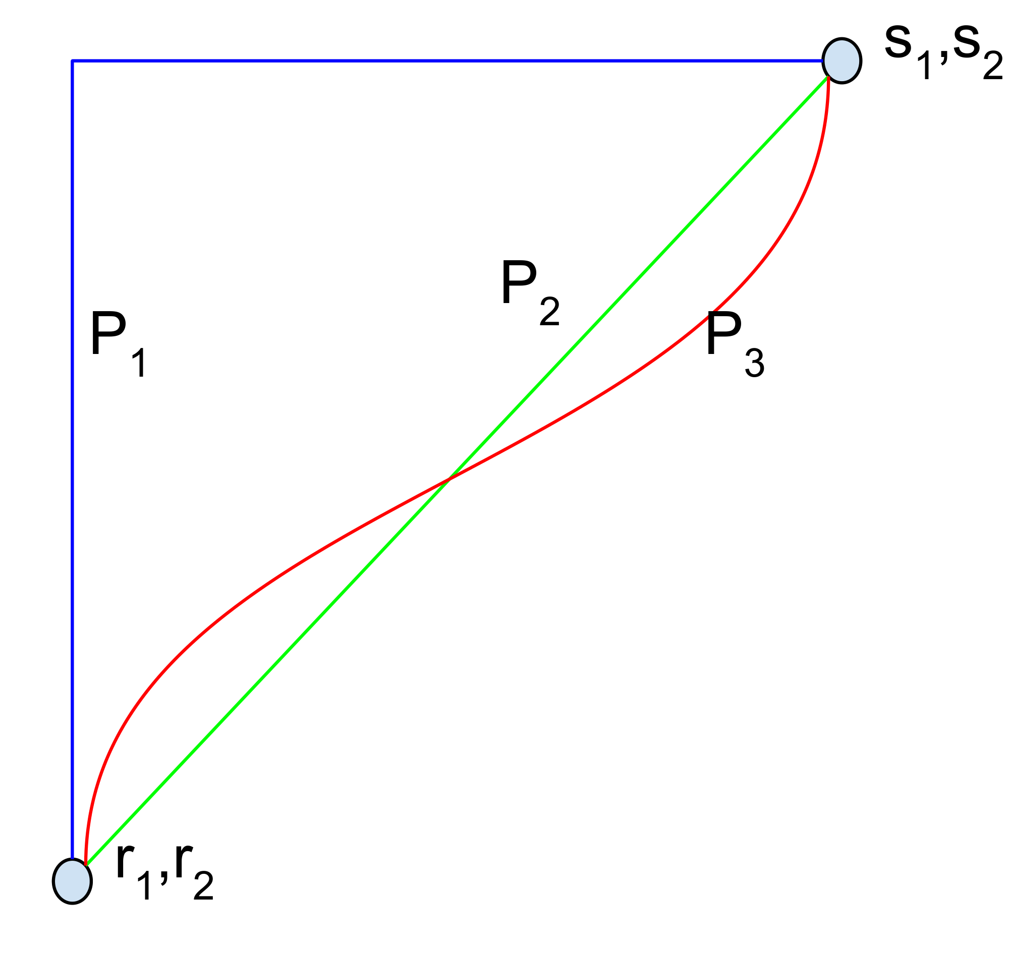
Formally, let $\gamma = (\gamma_1, \ldots, \gamma_n): [0, 1] \rightarrow \mathsf{R}^n$ be a smooth function specifying a path in $\mathsf{R}^n$ from the baseline $x'$ to the input $x$, i.e., $\gamma(0) = x'$ and $\gamma(1) = x$.

Given a path function $\gamma$, path integrated gradients are obtained by integrating the gradients along the path $\gamma(\alpha)$ for $\alpha \in [0, 1]$. Formally, path integrated gradients along the $i^{th}$ dimension for an input $x$ is defined as follows.

$ \mathsf{PathIntegratedGrads}^{\gamma}i(x) ::= \int{\alpha=0}^{1} \tfrac{\partial F(\gamma(\alpha))}{\partial \gamma_i(\alpha) }~\tfrac{\partial \gamma_i(\alpha)}{\partial \alpha} ~d \alpha $

where $\tfrac{\partial F(x)}{\partial x_i}$ is the gradient of $F$ along the $i^{th}$ dimension at $x$.

Attribution methods based on path integrated gradients are collectively known as path methods. Notice that integrated gradients is a path method for the straightline path specified $\gamma(\alpha) = x' + \alpha\times(x- x')$ for $\alpha \in [0, 1]$.

########## {caption="Remark"}

All path methods satisfy Implementation Invariance. This follows from the fact that they are defined using the underlying gradients, which do not depend on the implementation. They also satisfy Completeness (the proof is similar to that of Proposition 2) and Sensitvity(a) which is implied by Completeness (see Remark 3).

More interestingly, path methods are the only methods that satisfy certain desirable axioms. (For formal definitions of the axioms and proof of Proposition 4, see Friedman [9].)

Axiom: Sensitivity(b). (called Dummy in [9]) If the function implemented by the deep network does not depend (mathematically) on some variable, then the attribution to that variable is always zero.

This is a natural complement to the definition of Sensitivity(a) from Section 2. This definition captures desired insensitivity of the attributions.

Axiom: Linearity. Suppose that we linearly composed two deep networks modeled by the functions $f_1$ and $f_2$ to form a third network that models the function $a\times f_1 + b\times f_2$, i.e., a linear combination of the two networks. Then we'd like the attributions for $a\times f_1 + b\times f_2$ to be the weighted sum of the attributions for $f_1$ and $f_2$ with weights $a$ and $b$ respectively. Intuitively, we would like the attributions to preserve any linearity within the network.

########## {caption="Proposition 4"}

(Theorem 1 [9]) Path methods are the only attribution methods that always satisfy Implementation Invariance, Sensitivity(b), Linearity, and Completeness.

########## {caption="Remark"}

We note that these path integrated gradients have been used within the cost-sharing literature in economics where the function models the cost of a project as a function of the demands of various participants, and the attributions correspond to cost-shares. Integrated gradients correspond to a cost-sharing method called Aumann-Shapley [10]. Proposition 4 holds for our attribution problem because mathematically the cost-sharing problem corresponds to the attribution problem with the benchmark fixed at the zero vector. (Implementation Invariance is implicit in the cost-sharing literature as the cost functions are considered directly in their mathematical form.)

4.2 Integrated Gradients is Symmetry-Preserving

In this section, we formalize why the straightline path chosen by integrated gradients is canonical. First, observe that it is the simplest path that one can define mathematically. Second, a natural property for attribution methods is to preserve symmetry, in the following sense.

Symmetry-Preserving. Two input variables are symmetric w.r.t. a function if swapping them does not change the function. For instance, $x$ and $y$ are symmetric w.r.t. $F$ if and only if $F(x, y) = F(y, x)$ for all values of $x$ and $y$. An attribution method is symmetry preserving, if for all inputs that have identical values for symmetric variables and baselines that have identical values for symmetric variables, the symmetric variables receive identical attributions.

E.g., consider the logistic model $\mathsf{Sigmoid}(x_1+x_2+\dots)$. $x_1$ and $x_2$ are symmetric variables for this model. For an input where $x_1 = x_2 = 1$ (say) and baseline where $x_1 = x_2 = 0$ (say), a symmetry preserving method must offer identical attributions to $x_1$ and $x_2$.

It seems natural to ask for symmetry-preserving attribution methods because if two variables play the exact same role in the network (i.e., they are symmetric and have the same values in the baseline and the input) then they ought to receive the same attrbiution.

########## {caption="Theorem 5"}

Integrated gradients is the unique path method that is symmetry-preserving.

The proof is provided in Appendix A.

########## {caption="Remark"}

If we allow averaging over the attributions from multiple paths, then are other methods that satisfy all the axioms in Theorem 5. In particular, there is the method by Shapley-Shubik [11] from the cost sharing literature, and used by [12, 13] to compute feature attributions (though they were not studying deep networks). In this method, the attribution is the average of those from $n!$ extremal paths; here $n$ is the number of features. Here each such path considers an ordering of the input features, and sequentially changes the input feature from its value at the baseline to its value at the input. This method yields attributions that are different from integrated gradients. If the function of interest is $min(x_1, x_2)$, the baseline is $x_1=x_2=0$, and the input is $x_1 = 1$, $x_2 =3$, then integrated gradients attributes the change in the function value entirely to the critical variable $x_1$, whereas Shapley-Shubik assigns attributions of $1/2$ each; it seems somewhat subjective to prefer one result over the other.

We also envision other issues with applying Shapley-Shubik to deep networks: It is computationally expensive; in an object recognition network that takes an $100X100$ image as input, $n$ is $10000$, and $n!$ is a gigantic number. Even if one samples few paths randomly, evaluating the attributions for a single path takes $n$ calls to the deep network. In contrast, integrated gradients is able to operate with $20$ to $300$ calls. Further, the Shapley-Shubik computation visit inputs that are combinations of the input and the baseline. It is possible that some of these combinations are very different from anything seen during training. We speculate that this could lead to attribution artifacts.

5. Applying Integrated Gradients

Section Summary: When applying integrated gradients to explain AI model decisions, start by choosing a suitable baseline input that has a near-zero score and truly represents an absence of signal, such as a black image for object recognition tasks or an all-zero vector for text processing, to avoid misleading artifacts from adversarial examples. The method then approximates the integral by summing gradients calculated at regular intervals along a straight path from this baseline to the actual input, which can be efficiently done in a loop using deep learning tools like TensorFlow. In practice, 20 to 300 steps usually provide a good approximation, and you should verify accuracy by checking if the attributions add up to the difference between the model's score on the input and the baseline.

Selecting a Benchmark. A key step in applying integrated gradients is to select a good baseline. We recommend that developers check that the baseline has a near-zero score—as discussed in Section 3, this allows us to interpret the attributions as a function of the input. But there is more to a good baseline: For instance, for an object recogntion network it is possible to create an adversarial example that has a zero score for a given input label (say elephant), by applying a tiny, carefully-designed perturbation to an image with a very different label (say microscope) (cf. [14]). The attributions can then include undesirable artifacts of this adversarially constructed baseline. So we would additionally like the baseline to convey a complete absence of signal, so that the features that are apparent from the attributions are properties only of the input, and not of the baseline. For instance, in an object recognition network, a black image signifies the absence of objects. The black image isn't unique in this sense—an image consisting of noise has the same property. However, using black as a baseline may result in cleaner visualizations of "edge" features. For text based networks, we have found that the all-zero input embedding vector is a good baseline. The action of training causes unimportant words tend to have small norms, and so, in the limit, unimportance corresponds to the all-zero baseline. Notice that the black image corresponds to a valid input to an object recognition network, and is also intuitively what we humans would consider absence of signal. In contrast, the all-zero input vector for a text network does not correspond to a valid input; it nevertheless works for the mathematical reason described above.

Computing Integrated Gradients. The integral of integrated gradients can be efficiently approximated via a summation. We simply sum the gradients at points occurring at sufficiently small intervals along the straightline path from the baseline $x'$ to the input $x$.

$ \begin{split} \mathsf{IntegratedGrads}_i^{approx}(x) ::= \ (x_i- x'i)\times \Sigma{k=1}^m \tfrac{\partial F(x' + \tfrac{k}{m}\times(x- x')))}{\partial x_i}\times\tfrac{1}{m} \end{split} $

Here $m$ is the number of steps in the Riemman approximation of the integral. Notice that the approximation simply involves computing the gradient in a for loop which should be straightforward and efficient in most deep learning frameworks. For instance, in TensorFlow, it amounts to calling tf.gradients in a loop over the set of inputs (i.e., $x' + \tfrac{k}{m}\times(x- x')\text{for} k = 1, \ldots, m$), which could also be batched. In practice, we find that somewhere between $20$ and $300$ steps are enough to approximate the integral (within $5%$); we recommend that developers check that the attributions approximately adds up to the difference beween the score at the input and that at the baseline (cf. Proposition 2), and if not increase the step-size $m$.

6. Applications

Section Summary: The integrated gradients technique, which helps explain how AI models make decisions, is applied to various deep learning networks, including image recognition, natural language processing, and medical prediction systems. In object recognition, it highlights key pixels in photos that influence classifications, while in diabetic retinopathy detection, it pinpoints retinal lesions that affect severity predictions, aiding doctors in trusting and refining the model's outputs. For question classification and neural machine translation, it identifies important words or phrases that shape answers or align translated text, revealing both useful patterns and potential biases in the models.

The integrated gradients technique is applicable to a variety of deep networks. Here, we apply it to two image models, two natural language models, and a chemistry model.

6.1 An Object Recognition Network

We study feature attribution in an object recognition network built using the GoogleNet architecture [15] and trained over the ImageNet object recognition dataset [16]. We use the integrated gradients method to study pixel importance in predictions made by this network. The gradients are computed for the output of the highest-scoring class with respect to pixel of the input image. The baseline input is the black image, i.e., all pixel intensities are zero.

Integrated gradients can be visualized by aggregating them along the color channel and scaling the pixels in the actual image by them. Figure 2 shows visualizations for a bunch of images[^2]. For comparison, it also presents the corresponding visualization obtained from the product of the image with the gradients at the actual image. Notice that integrated gradients are better at reflecting distinctive features of the input image.

[^2]: More examples can be found at https://github.com/ankurtaly/Attributions

6.2 Diabetic Retinopathy Prediction

Diabetic retinopathy (DR) is a complication of the diabetes that affects the eyes. Recently, a deep network [17] has been proposed to predict the severity grade for DR in retinal fundus images. The model has good predictive accuracy on various validation datasets.

We use integrated gradients to study feature importance for this network; like in the object recognition case, the baseline is the black image. Feature importance explanations are important for this network as retina specialists may use it to build trust in the network's predictions, decide the grade for borderline cases, and obtain insights for further testing and screening.

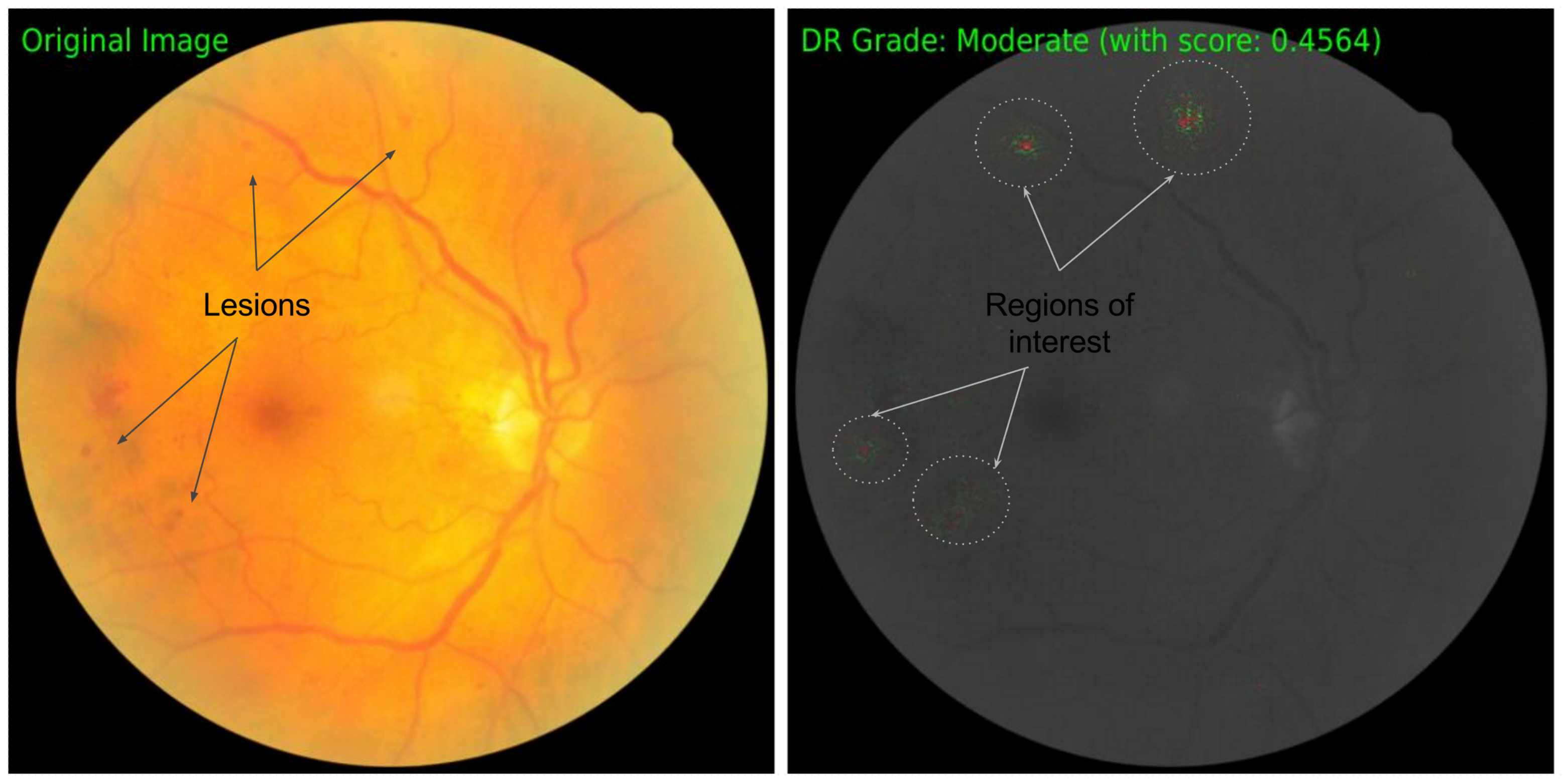
Figure 3 shows a visualization of integrated gradients for a retinal fundus image. The visualization method is a bit different from that used in Figure 2. We aggregate integrated gradients along the color channel and overlay them on the actual image in gray scale with positive attribtutions along the green channel and negative attributions along the red channel. Notice that integrated gradients are localized to a few pixels that seem to be lesions in the retina. The interior of the lesions receive a negative attribution while the periphery receives a positive attribution indicating that the network focusses on the boundary of the lesion.

6.3 Question Classification

Automatically answering natural language questions (over semi-structured data) is an important problem in artificial intelligence (AI). A common approach is to semantically parse the question to its logical form [18] using a set of human-authored grammar rules. An alternative approach is to machine learn an end-to-end model provided there is enough training data. An interesting question is whether one could peek inside machine learnt models to derive new rules. We explore this direction for a sub-problem of semantic parsing, called question classification, using the method of integrated gradients.

The goal of question classification is to identify the type of answer it is seeking. For instance, is the quesiton seeking a yes/no answer, or is it seeking a date? Rules for solving this problem look for trigger phrases in the question, for e.g., a "when" in the beginning indicates a date seeking question. We train a model for question classification using the the text categorization architecture proposed by [19] over the WikiTableQuestions dataset [20]. We use integrated gradients to attribute predictions down to the question terms in order to identify new trigger phrases for answer type. The baseline input is the all zero embedding vector.

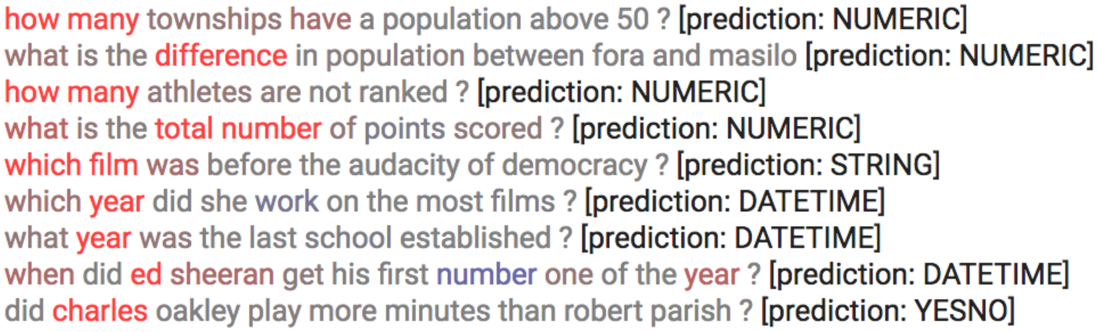
Figure 4 lists a few questions with constituent terms highlighted based on their attribution. Notice that the attributions largely agree with commonly used rules, for e.g., "how many" indicates a numeric seeking question. In addition, attributions help identify novel question classification rules, for e.g., questions containing "total number" are seeking numeric answers. Attributions also point out undesirable correlations, for e.g., "charles" is used as trigger for a yes/no question.

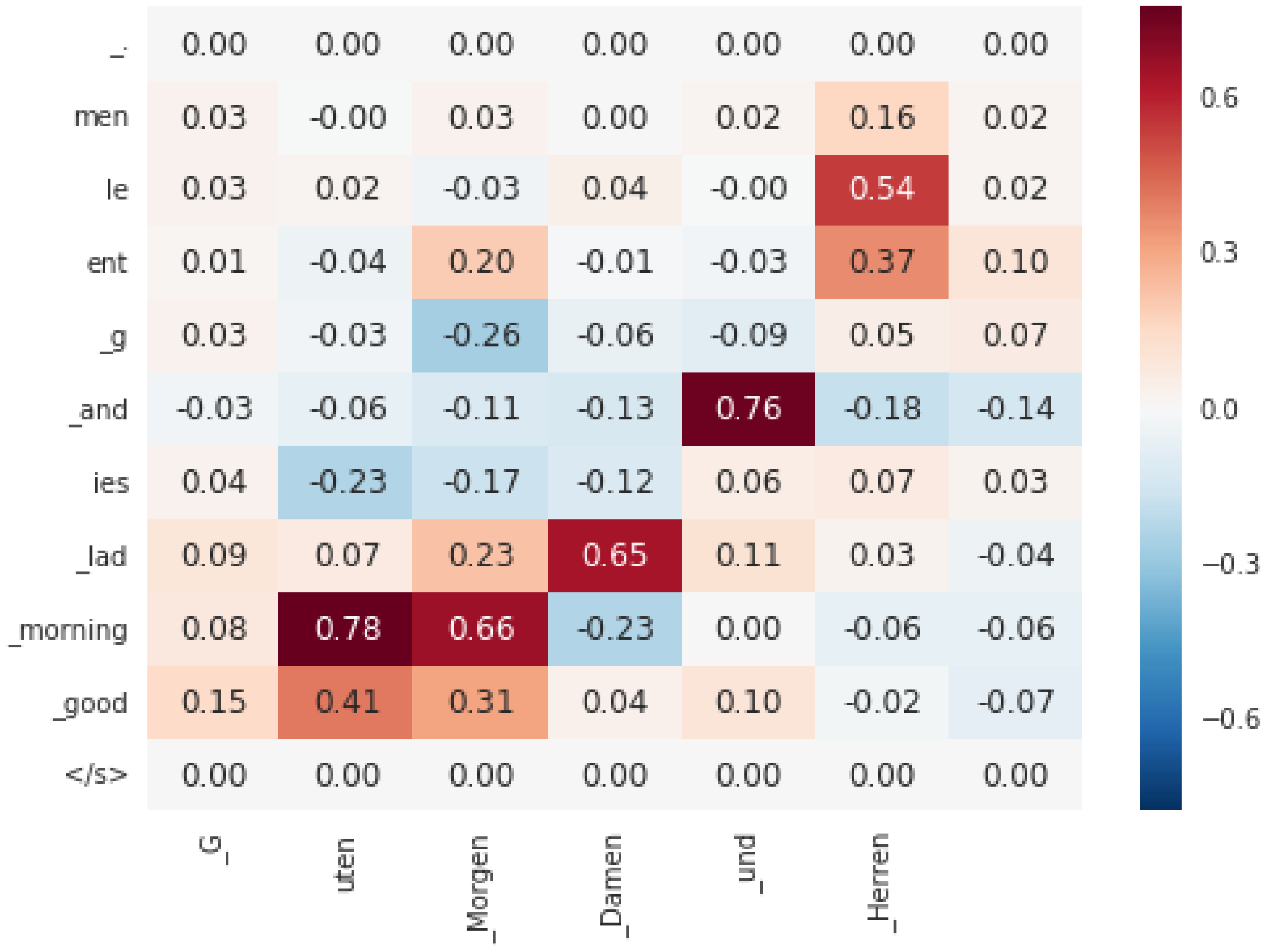
6.4 Neural Machine Translation

We applied our technique to a complex, LSTM-based Neural Machine Translation System [21]. We attribute the output probability of every output token (in form of wordpieces) to the input tokens. Such attributions "align" the output sentence with the input sentence. For baseline, we zero out the embeddings of all tokens except the start and end markers. Figure 5 shows an example of such an attribution-based alignments. We observed that the results make intuitive sense. E.g. "und" is mostly attributed to "and", and "morgen" is mostly attributed to "morning". We use $100-1000$ steps (cf. Section 5) in the integrated gradient approximation; we need this because the network is highly nonlinear.

6.5 Chemistry Models

We apply integrated gradients to a network performing Ligand-Based Virtual Screening which is the problem of predicting whether an input molecule is active against a certain target (e.g., protein or enzyme). In particular, we consider a network based on the molecular graph convolution architecture proposed by [22].

The network requires an input molecule to be encoded by hand as a set of atom and atom-pair features describing the molecule as an undirected graph. Atoms are featurized using a one-hot encoding specifying the atom type (e.g., C, O, S, etc.), and atom-pairs are featurized by specifying either the type of bond (e.g., single, double, triple, etc.) between the atoms, or the graph distance between them. The baseline input is obtained zeroing out the feature vectors for atom and atom-pairs.

We visualize integrated gradients as heatmaps over the the atom and atom-pair features with the heatmap intensity depicting the strength of the contribution. Figure 6 shows the visualization for a specific molecule. Since integrated gradients add up to the final prediction score (see Proposition 2), the magnitudes can be use for accounting the contributions of each feature. For instance, for the molecule in the figure, atom-pairs that have a bond between them cumulatively contribute to $46%$ of the prediction score, while all other pairs cumulatively contribute to only $-3%$.

:::: {cols="1"}

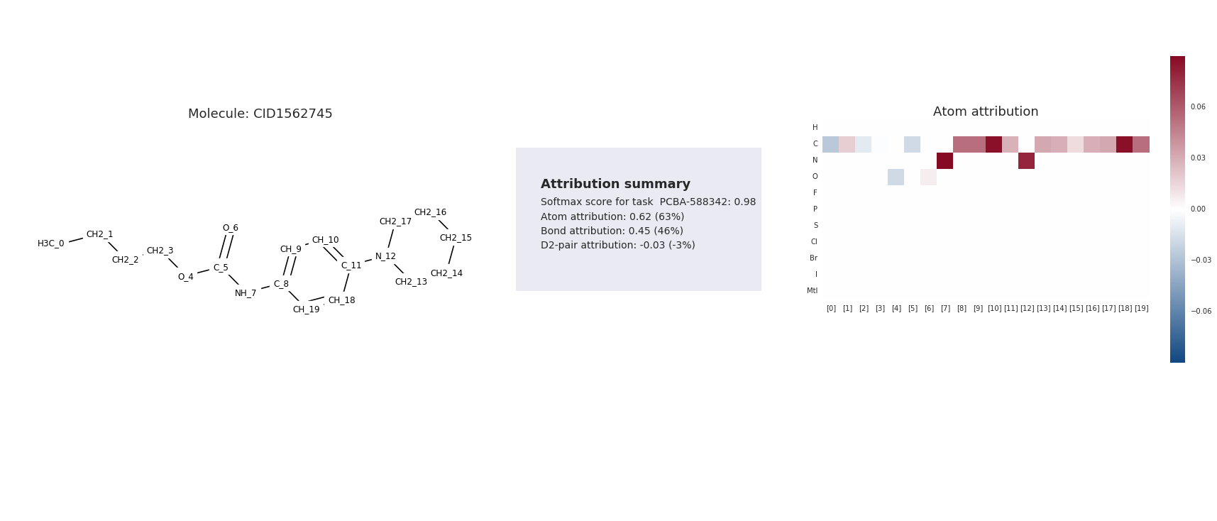
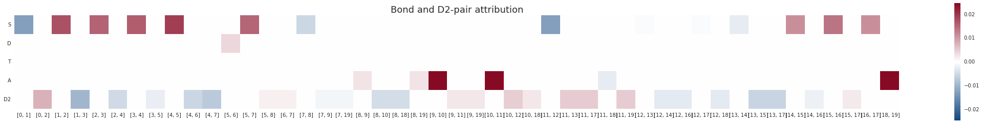
Figure 6: Attribution for a molecule under the W2N2 network [22]. The molecules is active on task PCBA-58432. ::::

Identifying Degenerate Features. We now discuss how attributions helped us spot an anomaly in the W1N2 architecture in [22]. On applying the integrated gradients method to this network, we found that several atoms in the same molecule received identical attribution despite being bonded to different atoms. This is surprising as one would expect two atoms with different neighborhoods to be treated differently by the network.

On investigating the problem further, in the network architecture, the atoms and atom-pair features were not fully convolved. This caused all atoms that have the same atom type, and same number of bonds of each type to contribute identically to the network.

7. Other Related work

Section Summary: Over the past few years, researchers have done extensive work to understand how deep neural networks operate internally, especially for image recognition tasks, by examining what individual neurons do or how they represent information during predictions. In contrast, this study focuses on explaining a network's decisions for a particular input by measuring the importance of basic input features. It also reviews related methods like local approximations, which simplify the network's behavior near the input but can be unreliable and computationally heavy for complex data, and attention mechanisms, which are popular but incomplete as they overlook other ways inputs affect outputs.

We already covered closely related work on attribution in Section 2. We mention other related work. Over the last few years, there has been a vast amount work on demystifying the inner workings of deep networks. Most of this work has been on networks trained on computer vision tasks, and deals with understanding what a specific neuron computes [23, 24] and interpreting the representations captured by neurons during a prediction [25, 26, 27]. In contrast, we focus on understanding the network's behavior on a specific input in terms of the base level input features. Our technique quantifies the importance of each feature in the prediction.

One approach to the attribution problem proposed first by [28, 29], is to locally approximate the behavior of the network in the vicinity of the input being explained with a simpler, more interpretable model. An appealing aspect of this approach is that it is completely agnostic to the implementation of the network and satisfies implemenation invariance. However, this approach does not guarantee sensitivity. There is no guarantee that the local region explored escapes the "flat" section of the prediction function in the sense of Section 2. The other issue is that the method is expensive to implement for networks with "dense" input like image networks as one needs to explore a local region of size proportional to the number of pixels and train a model for this space. In contrast, our technique works with a few calls to the gradient operation.

Attention mechanisms [30] have gained popularity recently. One may think that attention could be used a proxy for attributions, but this has issues. For instance, in a LSTM that also employs attention, there are many ways for an input token to influence an output token: the memory cell, the recurrent state, and "attention". Focussing only an attention ignores the other modes of influence and results in an incomplete picture.

8. Conclusion

Section Summary: This paper's main achievement is a technique called integrated gradients, which explains how deep learning networks make predictions by linking them back to the input data; it's simple to apply using basic math operations, works on many types of networks, and is backed by solid theory. It also introduces a set of principles, drawn from economics, to evaluate these explanation methods and ensure they're not skewed by flaws in the data, network, or method itself. While this advances understanding of which input features matter most, it doesn't yet explore how features interact or the reasoning inside networks, leaving room for further research on troubleshooting their behavior.

The primary contribution of this paper is a method called integrated gradients that attributes the prediction of a deep network to its inputs. It can be implemented using a few calls to the gradients operator, can be applied to a variety of deep networks, and has a strong theoretical justification.

A secondary contribution of this paper is to clarify desirable features of an attribution method using an axiomatic framework inspired by cost-sharing literature from economics. Without the axiomatic approach it is hard to tell whether the attribution method is affected by data artifacts, network's artifacts or artifacts of the method. The axiomatic approach rules out artifacts of the last type.

While our and other works have made some progress on understanding the relative importance of input features in a deep network, we have not addressed the interactions between the input features or the logic employed by the network. So there remain many unanswered questions in terms of debugging the I/O behavior of a deep network.

Acknowledgments

We would like to thank Samy Bengio, Kedar Dhamdhere, Scott Lundberg, Amir Najmi, Kevin McCurley, Patrick Riley, Christian Szegedy, Diane Tang for their feedback. We would like to thank Daniel Smilkov and Federico Allocati for identifying bugs in our descriptions. We would like to thank our anonymous reviewers for identifying bugs, and their suggestions to improve presentation.

Appendix

Section Summary: The appendix begins with a rigorous proof for Theorem 5, which uses a constructed path and function to show that attributions in certain neural network interpretation methods remain fair and equal for symmetrically treated input features, avoiding contradictions in importance assignment. It then provides counterexamples illustrating flaws in other popular techniques: DeepLift and Layer-wise Relevance Propagation yield inconsistent results for mathematically equivalent networks, as shown in a figure comparing two ReLU-based models, while Deconvolution and Guided Back-Propagation fail to detect sensitivity to inputs that clearly affect outputs. The section concludes with a list of references to key studies on neural network interpretability.

A. Proof of Theorem 5

Proof: Consider a non-straightline path $\gamma:[0, 1]\to \mathsf{R}^n$ from baseline to input. W.l.o.g., there exists $t_0\in [0, 1]$ such that for two dimensions $i, j$, $\gamma_i(t_0) > \gamma_j(t_0)$. Let $(t_1, t_2)$ be the maximum real open interval containing $t_0$ such that $\gamma_i(t) > \gamma_j(t)$ for all $t$ in $(t_1, t_2)$, and let $a= \gamma_i(t_1)= \gamma_j(t_1)$, and $b= \gamma_i(t_2)= \gamma_j(t_2)$. Define function $f:x\in [0, 1]^n\to R$ as $0$ if $\min(x_i, x_j) \leq a$, as $(b - a)^2$ if $\max(x_i, x_j)\geq b$, and as $(x_i - a)(x_j-a)$ otherwise. Next we compute the attributions of $f$ at $x=\langle 1, \ldots, 1\rangle_n$ with baseline $x'=\langle 0, \ldots, 0\rangle_n$. Note that $x_i$ and $x_j$ are symmetric, and should get identical attributions. For $t\notin [t_1, t_2]$, the function is a constant, and the attribution of $f$ is zero to all variables, while for $t\in(t_1, t_2)$, the integrand of attribution of $f$ is $\gamma_j(t) - a$ to $x_i$, and $\gamma_i(t) - a$ to $x_j$, where the latter is always strictly larger by our choice of the interval. Integrating, it follows that $x_j$ gets a larger attribution than $x_i$, contradiction.

B. Attribution Counter-Examples

We show that the methods DeepLift and Layer-wise relevance propagation (LRP) break the implementation invariance axiom, and the Deconvolution and Guided back-propagation methods break the sensitivity axiom.

Figure 10 provides an example of two equivalent networks $f(x_1, x_2)$ and $g(x_1, x_2)$ for which DeepLift and LRP yield different attributions.

First, observe that the networks $f$ and $g$ are of the form $f(x_1, x_2) = \mathsf{ReLU}(h(x_1, x_2))$ and $f(x_1, x_2) = \mathsf{ReLU}(k(x_1, x_2))$ [^3], where

$ \begin{array}{l} h(x_1, x_2) = \mathsf{ReLU}(x_1) - 1 - \mathsf{ReLU}(x_2) \ k(x_1, x_2) = \mathsf{ReLU}(x_1 - 1) - \mathsf{ReLU}(x_2) \end{array} $

Note that $h$ and $k$ are not equivalent. They have different values whenever $x_1<1$. But $f$ and $g$ are equivalent. To prove this, suppose for contradiction that $f$ and $g$ are different for some $x_1, x_2$. Then it must be the case that $\mathsf{ReLU}(x_1) - 1 \neq \mathsf{ReLU}(x_1 - 1)$. This happens only when $x_1<1$, which implies that $f(x_1, x_2)=g(x_1, x_2)=0$.

[^3]: $\mathsf{ReLU}(x)$ is defined as $\mathsf{max}(x, 0)$.

Now we leverage the above example to show that Deconvolution and Guided back-propagation break sensitivity. Consider the network $f(x_1, x_2$) from Figure 10. For a fixed value of $x_1$ greater than $1$, the output decreases linearly as $x_2$ increases from $0$ to $x_1 - 1$. Yet, for all inputs, Deconvolutional networks and Guided back-propagation results in zero attribution for $x_2$. This happens because for all inputs the back-propagated signal received at the node $\mathsf{ReLU}(x_2)$ is negative and is therefore not back-propagated through the $\mathsf{ReLU}$ operation (per the rules of deconvolution and guided back-propagation; see [5] for details). As a result, the feature $x_2$ receives zero attribution despite the network's output being sensitive to it.

References

[1] Baehrens, David, Schroeter, Timon, Harmeling, Stefan, Kawanabe, Motoaki, Hansen, Katja, and Müller, Klaus-Robert. How to explain individual classification decisions. Journal of Machine Learning Research, pp. 1803–1831, 2010.

[2] Simonyan, Karen, Vedaldi, Andrea, and Zisserman, Andrew. Deep inside convolutional networks: Visualising image classification models and saliency maps. CoRR, 2013.

[3] Shrikumar, Avanti, Greenside, Peyton, Shcherbina, Anna, and Kundaje, Anshul. Not just a black box: Learning important features through propagating activation differences. CoRR, 2016.

[4] Binder, Alexander, Montavon, Grégoire, Bach, Sebastian, Müller, Klaus-Robert, and Samek, Wojciech. Layer-wise relevance propagation for neural networks with local renormalization layers. CoRR, 2016.

[5] Springenberg, Jost Tobias, Dosovitskiy, Alexey, Brox, Thomas, and Riedmiller, Martin A. Striving for simplicity: The all convolutional net. CoRR, 2014.

[6] Shrikumar, Avanti, Greenside, Peyton, and Kundaje, Anshul. Learning important features through propagating activation differences. CoRR, abs/1704.02685, 2017. URL http://arxiv.org/abs/1704.02685.

[7] Zeiler, Matthew D. and Fergus, Rob. Visualizing and understanding convolutional networks. In ECCV, pp. 818–833, 2014.

[8] Samek, Wojciech, Binder, Alexander, Montavon, Grégoire, Bach, Sebastian, and Müller, Klaus-Robert. Evaluating the visualization of what a deep neural network has learned. CoRR, 2015.

[9] Friedman, Eric J. Paths and consistency in additive cost sharing. International Journal of Game Theory, 32(4):501–518, 2004.

[10] Aumann, R. J. and Shapley, L. S. Values of Non-Atomic Games. Princeton University Press, Princeton, NJ, 1974.

[11] Shapley, Lloyd S. and Shubik, Martin. The assignment game : the core. International Journal of Game Theory, 1(1):111–130, 1971. URL http://dx.doi.org/10.1007/BF01753437.

[12] Lundberg, Scott and Lee, Su-In. An unexpected unity among methods for interpreting model predictions. CoRR, abs/1611.07478, 2016. URL http://arxiv.org/abs/1611.07478.

[13] Datta, A., Sen, S., and Zick, Y. Algorithmic transparency via quantitative input influence: Theory and experiments with learning systems. In 2016 IEEE Symposium on Security and Privacy (SP), pp. 598–617, 2016.

[14] Goodfellow, Ian, Shlens, Jonathon, and Szegedy, Christian. Explaining and harnessing adversarial examples. In International Conference on Learning Representations, 2015. URL http://arxiv.org/abs/1412.6572.

[15] Szegedy, Christian, Liu, Wei, Jia, Yangqing, Sermanet, Pierre, Reed, Scott E., Anguelov, Dragomir, Erhan, Dumitru, Vanhoucke, Vincent, and Rabinovich, Andrew. Going deeper with convolutions. CoRR, 2014.

[16] Russakovsky, Olga, Deng, Jia, Su, Hao, Krause, Jonathan, Satheesh, Sanjeev, Ma, Sean, Huang, Zhiheng, Karpathy, Andrej, Khosla, Aditya, Bernstein, Michael, Berg, Alexander C., and Fei-Fei, Li. ImageNet Large Scale Visual Recognition Challenge. International Journal of Computer Vision (IJCV), pp. 211–252, 2015.

[17] Gulshan, Varun, Peng, Lily, Coram, Marc, and et al. Development and validation of a deep learning algorithm for detection of diabetic retinopathy in retinal fundus photographs. JAMA, 316(22):2402–2410, 2016.

[18] Liang, Percy. Learning executable semantic parsers for natural language understanding. Commun. ACM, 59(9):68–76, 2016.

[19] Kim, Yoon. Convolutional neural networks for sentence classification. In ACL, 2014.

[20] Pasupat, Panupong and Liang, Percy. Compositional semantic parsing on semi-structured tables. In ACL, 2015.

[21] Wu, Yonghui, Schuster, Mike, Chen, Zhifeng, Le, Quoc V., Norouzi, Mohammad, Macherey, Wolfgang, Krikun, Maxim, Cao, Yuan, Gao, Qin, Macherey, Klaus, Klingner, Jeff, Shah, Apurva, Johnson, Melvin, Liu, Xiaobing, Kaiser, Lukasz, Gouws, Stephan, Kato, Yoshikiyo, Kudo, Taku, Kazawa, Hideto, Stevens, Keith, Kurian, George, Patil, Nishant, Wang, Wei, Young, Cliff, Smith, Jason, Riesa, Jason, Rudnick, Alex, Vinyals, Oriol, Corrado, Greg, Hughes, Macduff, and Dean, Jeffrey. Google's neural machine translation system: Bridging the gap between human and machine translation. CoRR, abs/1609.08144, 2016. URL http://arxiv.org/abs/1609.08144.

[22] Kearnes, Steven, McCloskey, Kevin, Berndl, Marc, Pande, Vijay, and Riley, Patrick. Molecular graph convolutions: moving beyond fingerprints. Journal of Computer-Aided Molecular Design, pp. 595–608, 2016.

[23] Erhan, Dumitru, Bengio, Yoshua, Courville, Aaron, and Vincent, Pascal. Visualizing higher-layer features of a deep network. Technical Report 1341, University of Montreal, 2009.

[24] Le, Quoc V. Building high-level features using large scale unsupervised learning. In International Conference on Acoustics, Speech, and Signal Processing (ICASSP), pp. 8595–8598, 2013.

[25] Mahendran, Aravindh and Vedaldi, Andrea. Understanding deep image representations by inverting them. In Conference on Computer Vision and Pattern Recognition (CVPR), pp. 5188–5196, 2015.

[26] Dosovitskiy, Alexey and Brox, Thomas. Inverting visual representations with convolutional networks, 2015.

[27] Yosinski, Jason, Clune, Jeff, Nguyen, Anh Mai, Fuchs, Thomas, and Lipson, Hod. Understanding neural networks through deep visualization. CoRR, 2015.

[28] Ribeiro, Marco Túlio, Singh, Sameer, and Guestrin, Carlos. "why should I trust you?": Explaining the predictions of any classifier. In 22nd ACM International Conference on Knowledge Discovery and Data Mining, pp. 1135–1144. ACM, 2016a.

[29] Ribeiro, Marco Túlio, Singh, Sameer, and Guestrin, Carlos. Model-agnostic interpretability of machine learning. CoRR, 2016b.

[30] Bahdanau, Dzmitry, Cho, Kyunghyun, and Bengio, Yoshua. Neural machine translation by jointly learning to align and translate. CoRR, abs/1409.0473, 2014. URL http://arxiv.org/abs/1409.0473.