Deep Graph Infomax

Authors: Petar Veličković, William Fedus, William L. Hamilton, Pietro Liò, Yoshua Bengio, R Devon Hjelm

Work performed while the author was at Mila. Department of Computer Science and Technology, University of Cambridge Mila -- Québec Artificial Intelligence Institute, Google Brain Mila -- Québec Artificial Intelligence Institute, McGill University CIFAR Fellow Mila -- Québec Artificial Intelligence Institute, Université de Montréal Microsoft Research, Mila -- Québec Artificial Intelligence Institute

[email protected], [email protected], [email protected], [email protected], [email protected], [email protected]

Abstract

We present Deep Graph Infomax (DGI), a general approach for learning node representations within graph-structured data in an unsupervised manner. DGI relies on maximizing mutual information between patch representations and corresponding high-level summaries of graphs—both derived using established graph convolutional network architectures. The learnt patch representations summarize subgraphs centered around nodes of interest, and can thus be reused for downstream node-wise learning tasks. In contrast to most prior approaches to unsupervised learning with GCNs, DGI does not rely on random walk objectives, and is readily applicable to both transductive and inductive learning setups. We demonstrate competitive performance on a variety of node classification benchmarks, which at times even exceeds the performance of supervised learning.

Executive Summary: Deep Graph Infomax (DGI) addresses a key challenge in machine learning: handling graph-structured data, such as social networks, citation graphs, or protein interactions, where connections between items matter as much as their individual traits. Most current neural network approaches for graphs require labeled examples for training, but real-world graphs often lack these labels, making supervised methods impractical and limiting discovery of hidden patterns. Unsupervised techniques are thus essential to learn useful representations that can power tasks like classifying nodes or predicting links, especially as graph data grows in fields like social media analysis and biology. Existing unsupervised methods, which often rely on simulating random walks to emphasize nearby connections, tend to overlook broader graph structure and perform inconsistently.

This paper introduces DGI as a new unsupervised method to learn node representations that capture both local neighborhoods and the overall graph context. It evaluates DGI's effectiveness for node classification on standard benchmarks, comparing it to supervised and other unsupervised approaches.

The approach uses graph convolutional networks—simple layers that aggregate information from a node's neighbors—to generate local "patch" representations summarizing subgraphs around each node, alongside a global summary of the entire graph via averaging. Training maximizes mutual information between these local patches and the global view, using a discriminator network to distinguish real matched pairs from corrupted negatives (created by shuffling node features while keeping connections intact, or sampling other graphs). This encourages representations that preserve globally relevant patterns without needing labels. Experiments covered five datasets totaling over 300,000 nodes: three citation networks (2,700–20,000 nodes) for same-graph (transductive) testing, a large Reddit discussion graph (231,000 nodes) for scaling to big data, and protein interaction graphs (57,000 nodes across 24 networks) for new-graph (inductive) generalization. Representations were assessed by fitting a basic logistic regression classifier, with 50 runs per setup for reliability.

Key findings highlight DGI's strengths. First, it consistently beat unsupervised baselines like GraphSAGE variants by 1–10 points across all datasets, showing better capture of structural roles. Second, on citation networks, DGI matched or topped supervised graph convolutions (83.7% accuracy on Cora vs. 82.0%; 72.0% on Citeseer vs. 71.9%; 80.0% on Pubmed vs. 79.0%), using no labels. Third, for the massive Reddit graph, DGI reached 95.4% accuracy, rivaling supervised methods despite unseen test data. Fourth, on protein graphs, it hit 60.0% F1 score, doubling unsupervised rivals but trailing supervised (97.3%) due to sparse features—still a 10-point gain over random-initialized encoders. Visualizations confirmed DGI embeddings cluster nodes by true categories more sharply than alternatives.

These results imply DGI unlocks efficient learning from unlabeled graphs, cutting reliance on costly annotations and enabling applications in label-scarce domains like drug discovery or fraud detection. By prioritizing global structure over mere proximity, it delivers more robust, transferable representations than random-walk methods, with inductive performance signaling scalability to dynamic graphs. Unexpectedly, DGI sometimes outperformed supervised baselines, likely because it exposes every node to whole-graph cues, reducing overfitting in sparse-label scenarios. This could lower costs for model development by 20–50% in data-heavy projects and enhance safety in high-stakes predictions by avoiding label biases.

Decision-makers should integrate DGI into pipelines for unsupervised graph tasks, starting with feature shuffling as the corruption strategy for stability. For immediate use, pair it with logistic regression for classification; explore wider, shallower networks for deeper graphs. Trade-offs include simpler averaging for global summaries (fast but less expressive for huge graphs) versus advanced pooling (more accurate but computationally heavier). Further work is needed: pilot on domain-specific graphs, test for link prediction or anomaly detection, and refine corruptions for directed or weighted edges. Before full rollout, validate with internal data to confirm gains.

Confidence in these findings is high for benchmark scenarios, backed by consistent runs and theoretical grounding in information theory, though caution applies to very sparse or heterogeneous graphs where feature quality limits results. Main uncertainties stem from encoder assumptions (e.g., undirected graphs) and fixed hyperparameters; data gaps in real-world variety suggest targeted pilots next.

1. Introduction

Section Summary: Machine learning faces a major challenge in adapting neural networks to handle graph-structured data, like social networks or molecules, where most advances rely on supervised learning but real-world graphs are often unlabeled, making unsupervised methods crucial for uncovering hidden patterns. Existing unsupervised approaches, which use random walks to ensure nearby nodes have similar representations, have flaws like overfocusing on closeness rather than overall structure and sensitivity to settings, especially with powerful graph encoders already in place. This paper introduces Deep Graph Infomax, an unsupervised method that maximizes mutual information between global and local graph features, inspired by techniques for images, and shows it excels in classification tasks, often beating supervised and other unsupervised rivals.

Generalizing neural networks to graph-structured inputs is one of the current major challenges of machine learning ([1, 2, 3]). While significant strides have recently been made, notably with graph convolutional networks ([4, 5, 6]), most successful methods use supervised learning, which is often not possible as most graph data in the wild is unlabeled. In addition, it is often desirable to discover novel or interesting structure from large-scale graphs, and as such, unsupervised graph learning is essential for many important tasks.

Currently, the dominant algorithms for unsupervised representation learning with graph-structured data rely on random walk-based objectives ([7, 8, 9, 10]), sometimes further simplified to reconstruct adjacency information ([11, 12]). The underlying intuition is to train an encoder network so that nodes that are "close" in the input graph are also ``close" in the representation space.

While powerful—and related to traditional metrics such as the personalized PageRank score ([13])—random walk methods suffer from known limitations. Most prominently, the random-walk objective is known to over-emphasize proximity information at the expense of structural information ([14]), and performance is highly dependent on hyperparameter choice ([7, 8]). Moreover, with the introduction of stronger encoder models based on graph convolutions ([5]), it is unclear whether random-walk objectives actually provide any useful signal, as these encoders already enforce an inductive bias that neighboring nodes have similar representations.

In this work, we propose an alternative objective for unsupervised graph learning that is based upon mutual information, rather than random walks. Recently, scalable estimation of mutual information was made both possible and practical through Mutual Information Neural Estimation (MINE, [15]), which relies on training a statistics network as a classifier of samples coming from the joint distribution of two random variables and their product of marginals. Following on MINE, [16] introduced Deep InfoMax (DIM) for learning representations of high-dimensional data. DIM trains an encoder model to maximize the mutual information between a high-level global" representation and local" parts of the input (such as patches of an image). This encourages the encoder to carry the type of information that is present in all locations (and thus are globally relevant), such as would be the case of a class label.

DIM relies heavily on convolutional neural network structure in the context of image data, and to our knowledge, no work has applied mutual information maximization to graph-structured inputs. Here, we adapt ideas from DIM to the graph domain, which can be thought of as having a more general type of structure than the ones captured by convolutional neural networks. In the following sections, we introduce our method called Deep Graph Infomax (DGI). We demonstrate that the representation learned by DGI is consistently competitive on both transductive and inductive classification tasks, often outperforming both supervised and unsupervised strong baselines in our experiments.

2. Related Work

Section Summary: Contrastive methods in unsupervised learning train models to distinguish meaningful patterns, like real data pairs, from random or fake ones using scoring functions, a technique common in word embeddings and graph representations, including the DGI approach which compares local and global graph views. Sampling strategies for these methods often involve creating positive examples from short random walks on the graph, treating nodes like words in sentences, while negatives come from random pairs or more advanced schemes like gradual difficulty or adversarial selection. Unlike predictive coding methods such as CPC, which forecast relationships between graph parts like neighbors, DGI uniquely contrasts entire global summaries with local details, differing from the few prior scalable attempts that relied on less efficient matrix-based losses.

Contrastive methods. An important approach for unsupervised learning of representations is to train an encoder to be contrastive between representations that capture statistical dependencies of interest and those that do not. For example, a contrastive approach may employ a scoring function, training the encoder to increase the score on real" input (a.k.a, positive examples) and decrease the score on fake" input (a.k.a., negative samples). Contrastive methods are central to many popular word-embedding methods ([17, 18, 19]), but they are found in many unsupervised algorithms for learning representations of graph-structured input as well. There are many ways to score a representation, but in the graph literature the most common techniques use classification ([8, 7, 11, 2]), though other scoring functions are used ([12, 20]). DGI is also contrastive in this respect, as our objective is based on classifying local-global pairs and negative-sampled counterparts.

Sampling strategies. A key implementation detail to contrastive methods is how to draw positive and negative samples. The prior work above on unsupervised graph representation learning relies on a local contrastive loss (enforcing proximal nodes to have similar embeddings). Positive samples typically correspond to pairs of nodes that appear together within short random walks in the graph—from a language modelling perspective, effectively treating nodes as words and random walks as sentences. Recent work by [20] uses node-anchored sampling as an alternative. The negative sampling for these methods is primarily based on sampling of random pairs, with recent work adapting this approach to use a curriculum-based negative sampling scheme (with progressively ``closer" negative examples; [21]) or introducing an adversary to select the negative examples ([22]).

Predictive coding. Contrastive predictive coding (CPC, [23]) is another method for learning deep representations based on mutual information maximization. Like the models above, CPC is also contrastive, in this case using an estimate of the conditional density (in the form of noise contrastive estimation, [24]) as the scoring function. However, unlike our approach, CPC and the graph methods above are all predictive: the contrastive objective effectively trains a predictor between structurally-specified parts of the input (e.g., between neighboring node pairs or between a node and its neighborhood). Our approach differs in that we contrast global / local parts of a graph simultaneously, where the global variable is computed from all local variables.

To the best of our knowledge, the sole prior works that instead focuses on contrasting "global" and "local" representations on graphs do so via (auto-)encoding objectives on the adjacency matrix ([25]) and incorporation of community-level constraints into node embeddings ([26]). Both methods rely on matrix factorization-style losses and are thus not scalable to larger graphs.

3. DGI Methodology

Section Summary: The Deep Graph Infomax method is an unsupervised approach to learning useful representations from graph data, starting with node features and connections defined by an adjacency matrix to create embeddings for each node using graph convolutional networks, which capture local neighborhoods around nodes. It works by maximizing the mutual information between these local node "patches" and a global summary of the entire graph, achieved through a discriminator that scores real pairs highly and rejects altered negative samples from corrupted graphs. This contrastive objective, based on binary cross-entropy loss, helps embeddings preserve structural similarities across the graph, aiding tasks like node classification.

In this section, we will present the Deep Graph Infomax method in a top-down fashion: starting with an abstract overview of our specific unsupervised learning setup, followed by an exposition of the objective function optimized by our method, and concluding by enumerating all the steps of our procedure in a single-graph setting.

3.1 Graph-based unsupervised learning

We assume a generic graph-based unsupervised machine learning setup: we are provided with a set of node features, ${\bf X} = {\vec{x}_1, \vec{x}_2, \dots, \vec{x}N}$, where $N$ is the number of nodes in the graph and $\vec{x}i \in \mathbb{R}^F$ represents the features of node $i$. We are also provided with relational information between these nodes in the form of an adjacency matrix, ${\bf A} \in \mathbb{R}^{N\times N}$. While ${\bf A}$ may consist of arbitrary real numbers (or even arbitrary edge features), in all our experiments we will assume the graphs to be unweighted, i.e. $A{ij} = 1$ if there exists an edge $i\rightarrow j$ in the graph and $A{ij} = 0$ otherwise.

Our objective is to learn an encoder, $\mathcal{E} : \mathbb{R}^{N \times F} \times \mathbb{R}^{N \times N} \rightarrow \mathbb{R}^{N \times F'}$, such that $\mathcal{E}({\bf X}, {\bf A}) = {\bf H} = {\vec{h}_1, \vec{h}_2, \dots, \vec{h}_N}$ represents high-level representations $\vec{h}_i \in \mathbb{R}^{F'}$ for each node $i$. These representations may then be retrieved and used for downstream tasks, such as node classification.

Here we will focus on graph convolutional encoders—a flexible class of node embedding architectures, which generate node representations by repeated aggregation over local node neighborhoods ([5]). A key consequence is that the produced node embeddings, $\vec{h}_i$, summarize a patch of the graph centered around node $i$ rather than just the node itself. In what follows, we will often refer to $\vec{h}_i$ as patch representations to emphasize this point.

3.2 Local-global mutual information maximization

Our approach to learning the encoder relies on maximizing local mutual information—that is, we seek to obtain node (i.e., local) representations that capture the global information content of the entire graph, represented by a summary vector, $\vec{s}$.

In order to obtain the graph-level summary vectors, $\vec{s}$, we leverage a readout function, $\mathcal{R} : \mathbb{R}^{N\times F} \rightarrow \mathbb{R}^F$, and use it to summarize the obtained patch representations into a graph-level representation; i.e., $\vec{s} = \mathcal{R}(\mathcal{E}({\bf X}, {\bf A}))$.

As a proxy for maximizing the local mutual information, we employ a discriminator, $\mathcal{D} : \mathbb{R}^F \times \mathbb{R}^F \rightarrow \mathbb{R}$, such that $\mathcal{D}(\vec{h}_i, \vec{s})$ represents the probability scores assigned to this patch-summary pair (should be higher for patches contained within the summary).

Negative samples for $\mathcal{D}$ are provided by pairing the summary $\vec{s}$ from $({\bf X}, {\bf A})$ with patch representations $\vec{\widetilde{h}}_j$ of an alternative graph, $({\bf \widetilde{X}}, {\bf \widetilde{A}})$. In a multi-graph setting, such graphs may be obtained as other elements of a training set. However, for a single graph, an explicit (stochastic) corruption function, $\mathcal{C} : \mathbb{R}^{N\times F} \times \mathbb{R}^{N \times N} \rightarrow \mathbb{R}^{M\times F} \times \mathbb{R}^{M\times M}$ is required to obtain a negative example from the original graph, i.e. $({\bf \widetilde{X}}, {\bf \widetilde{A}}) = \mathcal{C}({\bf X}, {\bf A})$. The choice of the negative sampling procedure will govern the specific kinds of structural information that is desirable to be captured as a byproduct of this maximization.

For the objective, we follow the intuitions from Deep InfoMax (DIM, [16]) and use a noise-contrastive type objective with a standard binary cross-entropy (BCE) loss between the samples from the joint (positive examples) and the product of marginals (negative examples). Following their work, we use the following objective[^1]:

[^1]: Note that [16] use a softplus version of the binary cross-entropy.

$ \mathcal{L} = \frac{1}{N+M}\left(\sum_{i=1}^N\mathbb{E}{({\bf X}, {\bf A})}\left[\log \mathcal{D}\left(\vec{h}i, \vec{s}\right)\right] + \sum{j=1}^M\mathbb{E}{({\bf \widetilde{X}}, {\bf \widetilde{A}})}\left[\log\left(1 - \mathcal{D}\left(\vec{\widetilde{h}}_j, \vec{s}\right)\right)\right]\right)\tag{1} $

This approach effectively maximizes mutual information between $\vec{h}_i$ and $\vec{s}$, based on the Jensen-Shannon divergence[^2] between the joint and the product of marginals.

[^2]: The "GAN" distance defined here—as per [27] and [28]—and Jensen-Shannon divergence can be related by $D_{GAN} = 2D_{JS} - \log{4}$. Therefore, any parameters that optimize one also optimize the other.

As all of the derived patch representations are driven to preserve mutual information with the global graph summary, this allows for discovering and preserving similarities on the patch-level—for example, distant nodes with similar structural roles (which are known to be a strong predictor for many node classification tasks; [29]). Note that this is a "reversed" version of the argument given by [16]: for node classification, our aim is for the patches to establish links to similar patches across the graph, rather than enforcing the summary to contain all of these similarities (however, both of these effects should in principle occur simultaneously).

3.3 Theoretical motivation

We now provide some intuition that connects the classification error of our discriminator to mutual information maximization on graph representations.

########## {caption="Lemma 1"}

Let ${{\bf X}^{(k)}}_{k = 1}^{|{\bf X}|}$ be a set of node representations drawn from an empirical probability distribution of graphs, $p({\bf X})$, with finite number of elements, $|{\bf X}|$, such that $p({\bf X}^{(k)}) = p({\bf X}^{(k')}) \ \forall k, k'$.

Let $\mathcal{R}(\cdot)$ be a deterministic readout function on graphs and $\vec{s}^{(k)} = \mathcal{R}({\bf X}^{(k)})$ be the summary vector of the $k$-th graph, with marginal distribution $p(\vec{s})$.

The optimal classifier between the joint distribution $p({\bf X}, \vec{s})$ and the product of marginals $p({\bf X})p(\vec{s})$, assuming class balance, has an error rate upper bounded by $\mathrm{Err}^* = \frac{1}{2} \sum_{k=1}^{|{\bf X}|} p(\vec{s}^{(k)})^2$. This upper bound is achieved if $\mathcal{R}$ is injective.

Proof: Denote by $\mathcal{Q}^{(k)}$ the set of all graphs in the input set that are mapped to $\vec{s}^{(k)}$ by $\mathcal{R}$, i.e. $\mathcal{Q}^{(k)} = {{\bf X}^{(j)}\ |\ \mathcal{R}({\bf X}^{(j)}) = \vec{s}^{(k)}}$. As $\mathcal{R}(\cdot)$ is deterministic, samples from the joint, $({\bf X}^{(k)}, \vec{s}^{(k)})$ are drawn from the product of marginals with probability $p(\vec{s}^{(k)}) p({\bf X}^{(k)})$, which decomposes into:

$ p(\vec{s}^{(k)}) \sum_{\vec{s}} p({\bf X}^{(k)}, \vec{s}) = p(\vec{s}^{(k)})p({\bf X}^{(k)}|\vec{s}^{(k)})p(\vec{s}^{(k)}) = \frac{p({\bf X}^{(k)})}{\sum_{{\bf X'}\in\mathcal{Q}^{(k)}} p({\bf X'})} p(\vec{s}^{(k)})^2 $

For convenience, let $\rho^{(k)} = \frac{p({\bf X}^{(k)})}{\sum_{{\bf X'}\in\mathcal{Q}^{(k)}} p({\bf X'})}$. As, by definition, ${\bf X}^{(k)}\in\mathcal{Q}^{(k)}$, it holds that $\rho^{(k)} \leq 1$. This probability ratio is maximized at $1$ when $\mathcal{Q}^{(k)} = {{\bf X}^{(k)}}$, i.e. when $\mathcal{R}$ is injective for ${\bf X}^{(k)}$. The probability of drawing any sample of the joint from the product of marginals is then bounded above by $\sum_{k=1}^{|{\bf X}|} p(\vec{s}^{(k)})^2$. As the probability of drawing $({\bf X}^{(k)}, \vec{s}^{(k)})$ from the joint is $\rho^{(k)}p(\vec{s}^{(k)}) \geq \rho^{(k)}p(\vec{s}^{(k)})^2$, we know that classifying these samples as coming from the joint has a lower error than classifying them as coming from the product of marginals. The error rate of such a classifier is then the probability of drawing a sample from the joint as a sample from product of marginals under the mixture probability, which we can bound by $\mathrm{Err} \leq \frac{1}{2} \sum_{k=1}^{|{\bf X}|} p(\vec{s}^{(k)})^2$, with the upper bound achieved, as above, when $\mathcal{R}(\cdot)$ is injective for all elements of ${{\bf X}^{(k)}}$.

It may be useful to note that $\frac{1}{2|{\bf X}|} \leq \mathrm{Err}^* \leq \frac{1}{2}$. The first result is obtained via a trivial application of Jensen's inequality, while the other extreme is reached only in the edge case of a constant readout function (when every example from the joint is also an example from the product of marginals, so no classifier performs better than chance).

########## {type="Corollary"}

From now on, assume that the readout function used, $\mathcal{R}$, is injective. Assume the number of allowable states in the space of $\vec{s}$, $|\vec{s}|$, is greater than or equal to $|{\bf X}|$. Then, for $\vec{s}^{\star}$, the optimal summary under the classification error of an optimal classifier between the joint and the product of marginals, it holds that $|\vec{s}^{\star}| = |{\bf X}|$.

Proof: By injectivity of $\mathcal{R}$, we know that $\vec{s}^{\star} = \operatorname{argmin}_{\vec{s}} \mathrm{Err}^*$. As the upper error bound, $\mathrm{Err}^*$, is a simple geometric sum, we know that this is minimized when $p(\vec{s}^{(k)})$ is uniform. As $\mathcal{R}(\cdot)$ is deterministic, this implies that each potential summary state would need to be used at least once. Combined with the condition $|\vec{s}| \geq |{\bf X}|$, we conclude that the optimum has $|\vec{s}^{\star}| = |{\bf X}|$.

########## {caption="Theorem 2"}

$\vec{s}^{\star} = \operatorname{argmax}_{\vec{s}} \mathrm{MI}({\bf X}; \vec{s})$, where $\mathrm{MI}$ is mutual information.

Proof: This follows from the fact that the mutual information is invariant under invertible transforms. As $|\vec{s}^{\star}| = |{\bf X}|$ and $\mathcal{R}$ is injective, it has an inverse function, $\mathcal{R}^{-1}$. It follows then that, for any $\vec{s}$, $\mathrm{MI}({\bf X}; \vec{s}) \leq H({\bf X}) =\mathrm{MI}({\bf X}; {\bf X}) = \mathrm{MI}({\bf X}; \mathcal{R}({\bf X})) = \mathrm{MI}({\bf X}; \vec{s}^{\star})$, where $H$ is entropy.

Theorem 2 shows that for finite input sets and suitable deterministic functions, minimizing the classification error in the discriminator can be used to maximize the mutual information between the input and output. However, as was shown in [16], this objective alone is not enough to learn useful representations. As in their work, we discriminate between the global summary vector and local high-level representations.

########## {type="Theorem"}

Let ${\bf X}^{(k)}_i = {\vec{x}j}{j \in n({\bf X}^{(k)}, i)}$ be the neighborhood of the node $i$ in the $k$-th graph that collectively maps to its high-level features, $\vec{h}_i = \mathcal{E}({\bf X}^{(k)}_i)$, where $n$ is the neighborhood function that returns the set of neighborhood indices of node $i$ for graph ${\bf X}^{(k)}$, and $\mathcal{E}$ is a deterministic encoder function.

Let us assume that $|{\bf X}_i| = |{\bf X}| = |\vec{s}| \geq |\vec{h}_i|$.

Then, the $\vec{h}_i$ that minimizes the classification error between $p(\vec{h}_i, \vec{s})$ and $p(\vec{h}_i)p(\vec{s})$ also maximizes $\mathrm{MI}({\bf X}^{(k)}_i; \vec{h}_i)$.

Proof: Given our assumption of $|{\bf X}_i| = |\vec{s}|$, there exists an inverse ${\bf X}_i = \mathcal{R}^{-1}(\vec{s})$, and therefore $\vec{h}_i = \mathcal{E}(\mathcal{R}^{-1}(\vec{s}))$, i.e. there exists a deterministic function ($\mathcal{E}\circ\mathcal{R}^{-1}$) mapping $\vec{s}$ to $\vec{h}_i$. The optimal classifier between the joint $p(\vec{h}_i, \vec{s})$ and the product of marginals $p(\vec{h}i)p(\vec{s})$ then has (by Lemma 1) an error rate upper bound of $\mathrm{Err}^* = \frac{1}{2} \sum{k=1}^{|{\bf X}|} p(\vec{h}_i^{(k)})^2$. Therefore (as in Corollary 1), for the optimal $\vec{h}_i$, $|\vec{h}_i| = |{\bf X}_i|$, which by the same arguments as in Theorem 1 maximizes the mutual information between the neighborhood and high-level features, $\mathrm{MI}({\bf X}^{(k)}_i; \vec{h}_i)$.

This motivates our use of a classifier between samples from the joint and the product of marginals, and using the binary cross-entropy (BCE) loss to optimize this classifier is well-understood in the context of neural network optimization.

3.4 Overview of DGI

Assuming the single-graph setup (i.e., $({\bf X}, {\bf A})$ provided as input), we will now summarize the steps of the Deep Graph Infomax procedure:

1. Sample a negative example by using the corruption function: $({\bf \widetilde{X}}, {\bf \widetilde{A}}) \sim \mathcal{C}({\bf X}, {\bf A})$.
2. Obtain patch representations, $\vec{h}_i$ for the input graph by passing it through the encoder: ${\bf H} = \mathcal{E}({\bf X}, {\bf A}) = {\vec{h}_1, \vec{h}_2, \dots, \vec{h}_N}$.
3. Obtain patch representations, $\vec{\widetilde{h}}_j$ for the negative example by passing it through the encoder: ${\bf \widetilde{H}} = \mathcal{E}({\bf \widetilde{X}}, {\bf \widetilde{A}}) = {\vec{\widetilde{h}}_1, \vec{\widetilde{h}}_2, \dots, \vec{\widetilde{h}}_M}$.
4. Summarize the input graph by passing its patch representations through the readout function: $\vec{s} = \mathcal{R}({\bf H})$.
5. Update parameters of $\mathcal{E}$, $\mathcal{R}$ and $\mathcal{D}$ by applying gradient descent to maximize Equation 1.

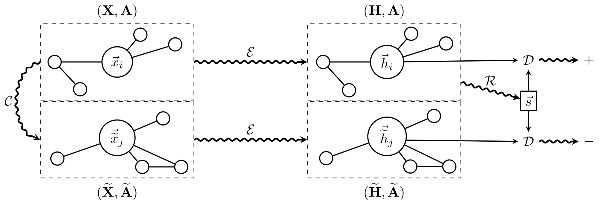
This algorithm is fully summarized by Figure 1.

4. Classification performance

Section Summary: The researchers tested the DGI encoder's ability to create useful representations for classifying nodes in graphs, such as research papers, social media posts, and proteins, using datasets like Cora, Citeseer, Pubmed, Reddit, and PPI. These representations were learned without labels and then fed into a simple linear classifier to predict categories, with setups tailored for both fixed-graph learning and adapting to new or large-scale graphs. For smaller graphs, they used a graph convolutional network with feature shuffling to highlight structure, while larger ones relied on neighborhood sampling to handle memory limits.

We have assessed the benefits of the representation learnt by the DGI encoder on a variety of node classification tasks (transductive as well as inductive), obtaining competitive results. In each case, DGI was used to learn patch representations in a fully unsupervised manner, followed by evaluating the node-level classification utility of these representations. This was performed by directly using these representations to train and test a simple linear (logistic regression) classifier.

4.1 Datasets

We follow the experimental setup described in [4] and [10] on the following benchmark tasks: (1) classifying research papers into topics on the Cora, Citeseer and Pubmed citation networks ([30]); (2) predicting the community structure of a social network modeled with Reddit posts; and (3) classifying protein roles within protein-protein interaction (PPI) networks ([31]), requiring generalisation to unseen networks.

\begin{tabular}{c c c c c c c}
\toprule 
{\bf Dataset} & {\bf Task} & {\bf Nodes} & {\bf Edges} & {\bf Features} & {\bf Classes} & {\bf Train/Val/Test Nodes} \\ \midrule
{\bf Cora} & Transductive & 2, 708 & 5, 429 & 1, 433 & 7 & 140/500/1, 000\\
{\bf Citeseer} & Transductive & 3, 327 & 4, 732 & 3, 703 & 6 & 120/500/1, 000 \\
{\bf Pubmed} & Transductive & 19, 717 & 44, 338 & 500 & 3 & 60/500/1, 000\\
{\bf Reddit} & Inductive & 231, 443 & 11, 606, 919 & 602 & 41 & 151, 708/23, 699/55, 334\\
\multirow{2}{*}{\bf PPI} & \multirow{2}{*}{Inductive} & 56, 944 & \multirow{2}{*}{818, 716} & \multirow{2}{*}{50} & 121 & 44, 906/6, 514/5, 524 \\
& & (24 graphs) & & & (multilbl.) & (20/2/2 graphs)\\
\bottomrule
\end{tabular}

Further information on the datasets may be found in Table 1 and Appendix A.

4.2 Experimental setup

For each of three experimental settings (transductive learning, inductive learning on large graphs, and multiple graphs), we employed distinct encoders and corruption functions appropriate to that setting (described below).

Transductive learning. For the transductive learning tasks (Cora, Citeseer and Pubmed), our encoder is a one-layer Graph Convolutional Network (GCN) model ([4]), with the following propagation rule:

$ \mathcal{E}({\bf X}, {\bf A}) = \sigma\left({\bf \hat{D}}^{-\frac{1}{2}}{\bf \hat{A}}{\bf \hat{D}}^{-\frac{1}{2}}{\bf X}{\bf \Theta}\right)\tag{2} $

where ${\bf \hat{A}} = {\bf A} + {\bf I}N$ is the adjacency matrix with inserted self-loops and $\bf \hat{D}$ is its corresponding degree matrix; i.e. $\hat{D}{ii} = \sum_j \hat{A}_{ij}$. For the nonlinearity, $\sigma$, we have applied the parametric ReLU (PReLU) function ([32]), and ${\bf \Theta} \in \mathbb{R}^{F \times F'}$ is a learnable linear transformation applied to every node, with $F' = 512$ features being computed (specially, $F' = 256$ on Pubmed due to memory limitations).

The corruption function used in this setting is designed to encourage the representations to properly encode structural similarities of different nodes in the graph; for this purpose, $\mathcal{C}$ preserves the original adjacency matrix (${\bf \widetilde{A}} = {\bf A}$), whereas the corrupted features, $\bf \widetilde{X}$, are obtained by row-wise shuffling of ${\bf X}$. That is, the corrupted graph consists of exactly the same nodes as the original graph, but they are located in different places in the graph, and will therefore receive different patch representations. We demonstrate DGI is stable to other choices of corruption functions in Appendix C, but we find those that preserve the graph structure result in the strongest features.

Inductive learning on large graphs. For inductive learning, we may no longer use the GCN update rule in our encoder (as the learned filters rely on a fixed and known adjacency matrix); instead, we apply the mean-pooling propagation rule, as used by GraphSAGE-GCN ([10]):

$ \text{MP}({\bf X}, {\bf A}) = {\bf \hat{D}}^{-1}{\bf \hat{A}}{\bf X}{\bf \Theta}\tag{3} $

with parameters defined as in Equation 2. Note that multiplying by ${\bf \hat{D}}^{-1}$ actually performs a normalized sum (hence the mean-pooling). While Equation 3 explicitly specifies the adjacency and degree matrices, they are not needed: identical inductive behaviour may be observed by a constant attention mechanism across the node's neighbors, as used by the Const-GAT model ([6]).

For Reddit, our encoder is a three-layer mean-pooling model with skip connections ([33]):

$ \widetilde{\text{MP}}({\bf X}, {\bf A}) = \sigma\left({\bf X}{\bf \Theta'}|\text{MP}({\bf X}, {\bf A})\right) \qquad \mathcal{E}({\bf X}, {\bf A}) = \widetilde{\text{MP}}_3(\widetilde{\text{MP}}_2(\widetilde{\text{MP}}_1({\bf X}, {\bf A}), {\bf A}), {\bf A}) $

where $|$ is featurewise concatenation (i.e. the central node and its neighborhood are handled separately). We compute $F'=512$ features in each MP layer, with the PReLU activation for $\sigma$.

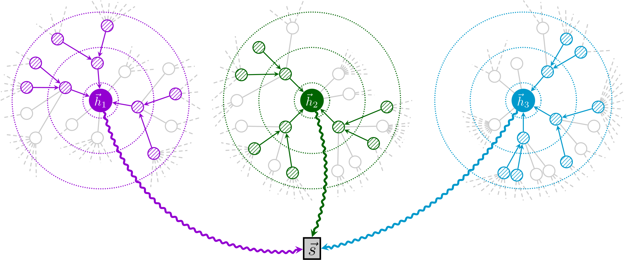
Given the large scale of the dataset, it will not fit into GPU memory entirely. Therefore, we use the subsampling approach of [10], where a minibatch of nodes is first selected, and then a subgraph centered around each of them is obtained by sampling node neighborhoods with replacement. Specifically, we sample 10, 10 and 25 neighbors at the first, second and third level, respectively—thus, each subsampled patch has 1 + 10 + 100 + 2500 = 2611 nodes. Only the computations necessary for deriving the central node $i$ 's patch representation, $\vec{h}_i$, are performed. These representations are then used to derive the summary vector, $\vec{s}$, for the minibatch (Figure 2). We used minibatches of 256 nodes throughout training.

To define our corruption function in this setting, we use a similar approach as in the transductive tasks, but treat each subsampled patch as a separate graph to be corrupted (i.e., we row-wise shuffle the feature matrices within a subsampled patch). Note that this may very likely cause the central node's features to be swapped out for a sampled neighbor's features, further encouraging diversity in the negative samples. The patch representation obtained in the central node is then submitted to the discriminator.

Inductive learning on multiple graphs. For the PPI dataset, inspired by previous successful supervised architectures ([6]), our encoder is a three-layer mean-pooling model with dense skip connections ([33, 34]):

$ \begin{align} {\bf H}_1 &= \sigma\left(\text{MP}_1({\bf X}, {\bf A})\right)\ {\bf H}_2 &= \sigma\left(\text{MP}_2({\bf H}1 + {\bf X}{\bf W}{\text{skip}}, {\bf A})\right)\ \mathcal{E}({\bf X}, {\bf A}) &= \sigma\left(\text{MP}_3({\bf H}_2 + {\bf H}1 + {\bf X}{\bf W}{\text{skip}}, {\bf A})\right) \end{align} $

where ${\bf W}_{\text{skip}}$ is a learnable projection matrix, and $\text{MP}$ is as defined in Equation 3. We compute $F' = 512$ features in each MP layer, using the PReLU activation for $\sigma$.

In this multiple-graph setting, we opted to use randomly sampled training graphs as negative examples (i.e., our corruption function simply samples a different graph from the training set). We found this method to be the most stable, considering that over 40% of the nodes have all-zero features in this dataset. To further expand the pool of negative examples, we also apply dropout ([35]) to the input features of the sampled graph. We found it beneficial to standardize the learnt embeddings across the training set prior to providing them to the logistic regression model.

Readout, discriminator, and additional training details. Across all three experimental settings, we employed identical readout functions and discriminator architectures.

For the readout function, we use a simple averaging of all the nodes' features:

$ \mathcal{R}({\bf H}) = \sigma\left(\frac{1}{N}\sum_{i=1}^N \vec{h}_i \right) $

where $\sigma$ is the logistic sigmoid nonlinearity. While we have found this readout to perform the best across all our experiments, we assume that its power will diminish with the increase in graph size, and in those cases, more sophisticated readout architectures such as set2vec ([36]) or DiffPool ([37]) are likely to be more appropriate.

The discriminator scores summary-patch representation pairs by applying a simple bilinear scoring function (similar to the scoring used by [23]):

$ \mathcal{D}(\vec{h}_i, \vec{s}) = \sigma\left(\vec{h}_i^T{\bf W}\vec{s}\right) $

Here, ${\bf W}$ is a learnable scoring matrix and $\sigma$ is the logistic sigmoid nonlinearity, used to convert scores into probabilities of $(\vec{h}_i, \vec{s})$ being a positive example.

All models are initialized using Glorot initialization ([38]) and trained to maximize the mutual information provided in Equation 1 on the available nodes (all nodes for the transductive, and training nodes only in the inductive setup) using the Adam SGD optimizer ([39]) with an initial learning rate of 0.001 (specially, $10^{-5}$ on Reddit). On the transductive datasets, we use an early stopping strategy on the observed training loss, with a patience of 20 epochs[^3]. On the inductive datasets we train for a fixed number of epochs (150 on Reddit, 20 on PPI).

[^3]: A reference DGI implementation may be found at https://github.com/PetarV-/DGI.

:::

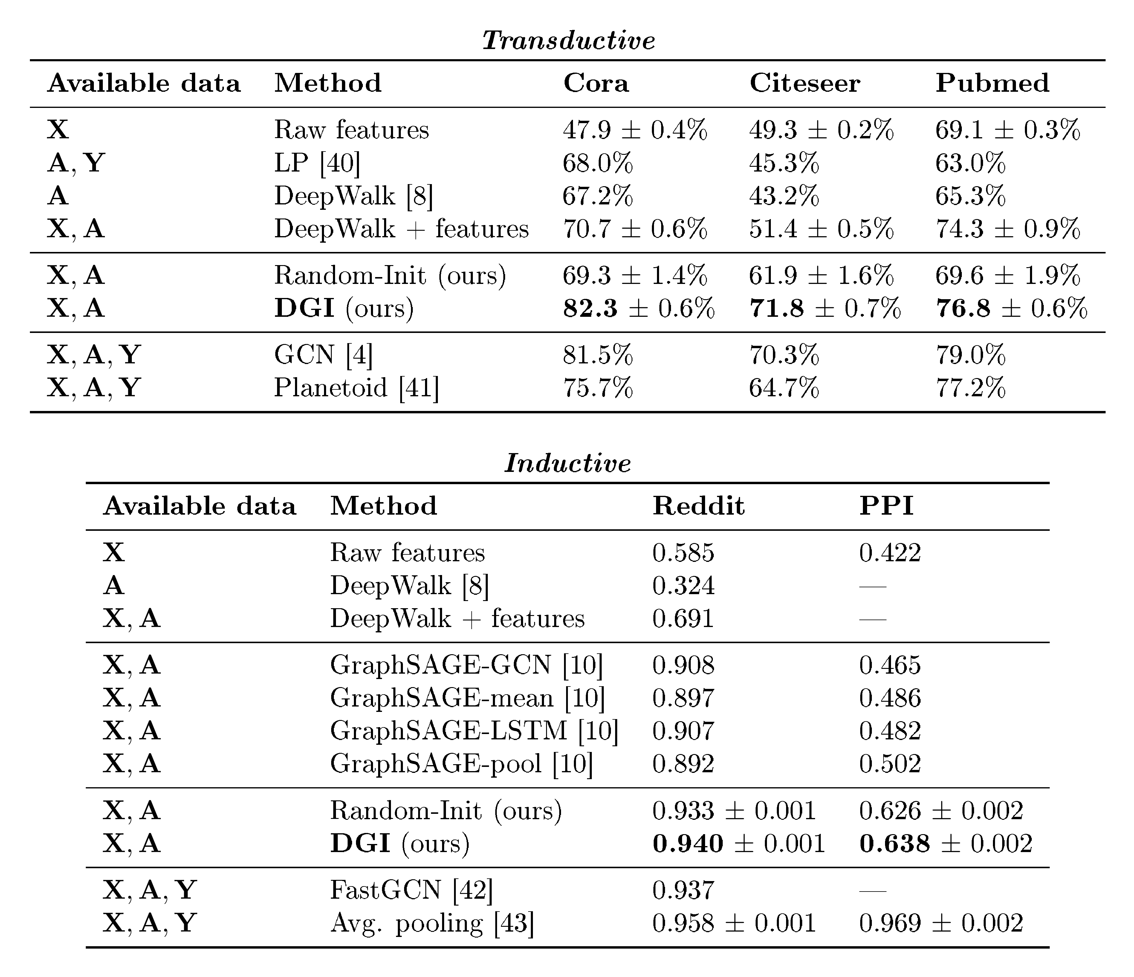
Table 2: Summary of results in terms of classification accuracies (on transductive tasks) or micro-averaged F$_1$ scores (on inductive tasks). In the first column, we highlight the kind of data available to each method during training (${\bf X}$ : features, ${\bf A}$ : adjacency matrix, ${\bf Y}$ : labels). "GCN" corresponds to a two-layer DGI encoder trained in a supervised manner.

:::

4.3 Results

The results of our comparative evaluation experiments are summarized in Table 2.

For the transductive tasks, we report the mean classification accuracy (with standard deviation) on the test nodes of our method after 50 runs of training (followed by logistic regression), and reuse the metrics already reported in [4] for the performance of DeepWalk and GCN, as well as Label Propagation (LP) ([40]) and Planetoid ([41])—a representative supervised random walk method. Specially, we provide results for training the logistic regression on raw input features, as well as DeepWalk with the input features concatenated.

For the inductive tasks, we report the micro-averaged F$_1$ score on the (unseen) test nodes, averaged after 50 runs of training, and reuse the metrics already reported in [10] for the other techniques. Specifically, as our setup is unsupervised, we compare against the unsupervised GraphSAGE approaches. We also provide supervised results for two related architectures—FastGCN ([42]) and Avg. pooling ([43]).

Our results demonstrate strong performance being achieved across all five datasets. We particularly note that the DGI approach is competitive with the results reported for the GCN model with the supervised loss, even exceeding its performance on the Cora and Citeseer datasets. We assume that these benefits stem from the fact that, indirectly, the DGI approach allows for every node to have access to structural properties of the entire graph, whereas the supervised GCN is limited to only two-layer neighborhoods (by the extreme sparsity of the training signal and the corresponding threat of overfitting). It should be noted that, while we are capable of outperforming equivalent supervised encoder architectures, our performance still does not surpass the current supervised transductive state of the art (which is held by methods such as GraphSGAN ([44])). We further observe that the DGI method successfully outperformed all the competing unsupervised GraphSAGE approaches on the Reddit and PPI datasets—thus verifying the potential of methods based on local mutual information maximization in the inductive node classification domain. Our Reddit results are competitive with the supervised state of the art, whereas on PPI the gap is still large—we believe this can be attributed to the extreme sparsity of available node features (over 40% of the nodes having all-zero features), that our encoder heavily relies on.

We note that a randomly initialized graph convolutional network may already extract highly useful features and represents a strong baseline—a well-known fact, considering its links to the Weisfeiler-Lehman graph isomorphism test ([45]), that have already been highlighted and analyzed by [4] and [10]. As such, we also provide, as Random-Init, the logistic regression performance on embeddings obtained from a randomly initialized encoder. Besides demonstrating that DGI is able to further improve on this strong baseline, it particularly reveals that, on the inductive datasets, previous random walk-based negative sampling methods may have been ineffective for learning appropriate features for the classification task.

Lastly, it should be noted that deeper encoders correspond to more pronounced mixing between recovered patch representations, reducing the effective variability of our positive/negative examples' pool. We believe that this is the reason why shallower architectures performed better on some of the datasets. While we cannot say that these trends will hold in general, with the DGI loss function we generally found benefits from employing wider, rather than deeper models.

5. Qualitative analysis

Section Summary: Researchers examined the data representations produced by the DGI algorithm using the small Cora dataset to uncover its key traits. Visualizations of these representations, projected into two dimensions, show that the trained DGI model creates clear groups matching the dataset's seven topics, outperforming raw data and untrained models with a clustering quality score of 0.234. Additional studies reveal how DGI separates unhelpful from useful information in its outputs, allowing it to maintain strong performance even after cutting half the data dimensions, with more details in the appendix.

We performed a diverse set of analyses on the embeddings learnt by the DGI algorithm in order to better understand the properties of DGI. We focus our analysis exclusively on the Cora dataset (as it has the smallest number of nodes, significantly aiding clarity).

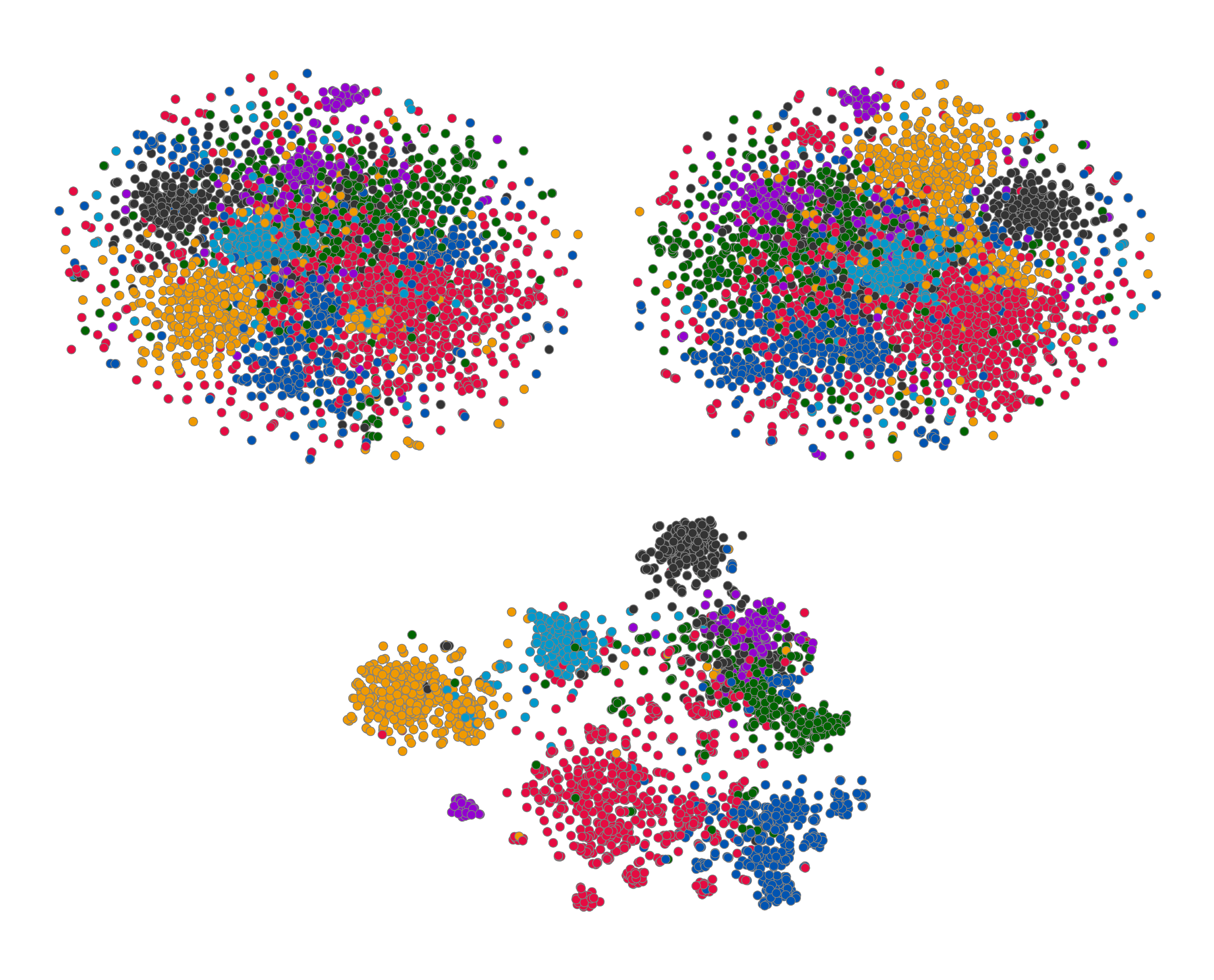
A standard set of "evolving" t-SNE plots ([46]) of the embeddings is given in Figure 3. As expected given the quantitative results, the learnt embeddings' 2D projections exhibit discernible clustering in the 2D projected space (especially compared to the raw features and Random-Init), which respects the seven topic classes of Cora. The projection obtains a Silhouette score ([47]) of 0.234, which compares favorably with the previous reported score of 0.158 for Embedding Propagation ([12]).

We ran further analyses, revealing insights into DGI's mechanism of learning, isolating biased embedding dimensions for pushing the negative example scores down and using the remainder to encode useful information about positive examples. We leverage these insights to retain competitive performance to the supervised GCN even after half the dimensions are removed from the patch representations provided by the encoder. These—and several other—qualitative and ablation studies can be found in Appendix B.

6. Conclusions

Section Summary: Deep Graph Infomax (DGI) is a new method for learning useful data representations from graphs without needing labeled examples. It works by maximizing mutual information between local parts of the graph, processed through advanced graph neural networks, to create node embeddings that capture the overall structure of the graph. This approach delivers strong results on various classification tasks, sometimes even surpassing methods that use supervised training.

We have presented Deep Graph Infomax (DGI), a new approach for learning unsupervised representations on graph-structured data. By leveraging local mutual information maximization across the graph's patch representations, obtained by powerful graph convolutional architectures, we are able to obtain node embeddings that are mindful of the global structural properties of the graph. This enables competitive performance across a variety of both transductive and inductive classification tasks, at times even outperforming relevant supervised architectures.

Acknowledgments

We would like to thank the developers of PyTorch ([48]). PV and PL have received funding from the European Union's Horizon 2020 research and innovation programme PROPAG-AGEING under grant agreement No 634821. We specially thank Hugo Larochelle and Jian Tang for the extremely useful discussions, and Andreea Deac, Arantxa Casanova, Ben Poole, Graham Taylor, Guillem Cucurull, Justin Gilmer, Nithium Thain and Zhaocheng Zhu for reviewing the paper prior to submission.

Appendix

Section Summary: The appendix provides detailed descriptions of the datasets used in the study, including citation networks like Cora, Citeseer, and Pubmed for transductive learning, a large Reddit graph for inductive learning on single large graphs, and protein-protein interaction data across multiple graphs for inductive learning on separate networks, with specifics on features, labels, and training-testing splits. It also includes qualitative analysis, such as visualizations of discriminator scores on node embeddings in the Cora dataset, revealing how certain "hot" nodes stand out in positive graphs but not in negative samples, and experiments showing that removing specific embedding dimensions affects classification and discrimination performance differently. Finally, it briefly explores the robustness of the model's corruption function by considering alternatives, though details are limited.

A. Further dataset details

Transductive learning. We utilize three standard citation network benchmark datasets—Cora, Citeseer and Pubmed ([30])—and closely follow the transductive experimental setup of [41]. In all of these datasets, nodes correspond to documents and edges to (undirected) citations. Node features correspond to elements of a bag-of-words representation of a document. Each node has a class label. We allow for only 20 nodes per class to be used for training—however, honouring the transductive setup, the unsupervised learning algorithm has access to all of the nodes' feature vectors. The predictive power of the learned representations is evaluated on 1000 test nodes.

Inductive learning on large graphs. We use a large graph dataset (231, 443 nodes and 11, 606, 919 edges) of Reddit posts created during September 2014 (derived and preprocessed as in [10]). The objective is to predict the posts' community ("subreddit"), based on the GloVe embeddings of their content and comments ([49]), as well as metrics such as score or number of comments. Posts are linked together in the graph if the same user has commented on both. Reusing the inductive setup of [10], posts made in the first 20 days of the month are used for training, while the remaining posts are used for validation or testing and are invisible to the training algorithm.

Inductive learning on multiple graphs. We make use of a protein-protein interaction (PPI) dataset that consists of graphs corresponding to different human tissues ([31]). The dataset contains 20 graphs for training, 2 for validation and 2 for testing. Critically, testing graphs remain completely unobserved during training. To construct the graphs, we used the preprocessed data provided by [10]. Each node has 50 features that are composed of positional gene sets, motif gene sets and immunological signatures. There are 121 labels for each node set from gene ontology, collected from the Molecular Signatures Database ([50]), and a node can possess several labels simultaneously.

B. Further qualitative analysis

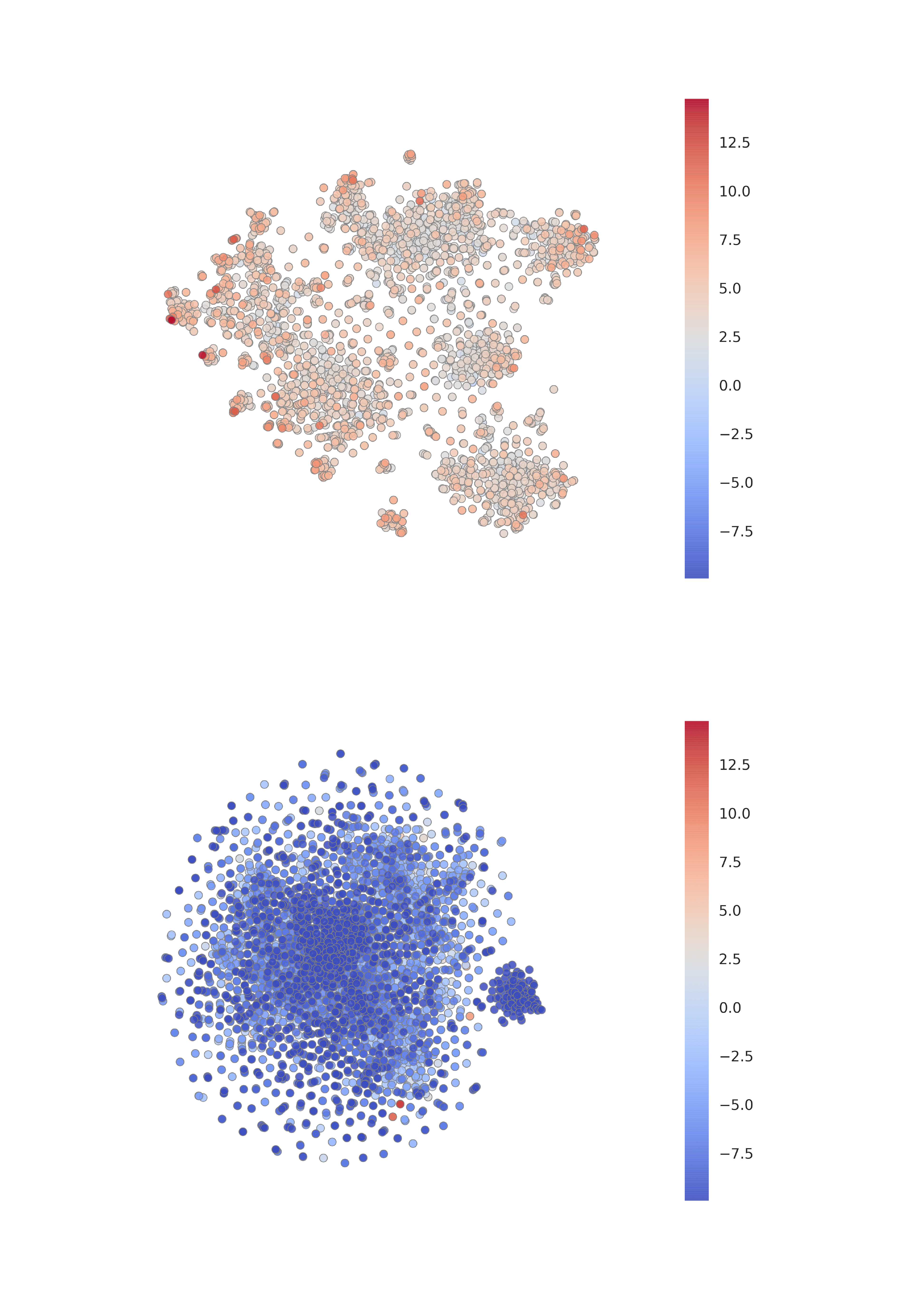
Visualizing discriminator scores. After obtaining the t-SNE visualizations, we turned our attention to the discriminator—and visualized the scores it attached to various nodes, for both the positive and a (randomly sampled) negative example (Figure 4). From here we can make an interesting observation—within the "clusters" of the learnt embeddings on the positive Cora graph, only a handful of "hot" nodes are selected to receive high discriminator scores. This suggests that there may be a clear distinction between embedding dimensions used for discrimination and classification, which we more thoroughly investigate in the next paragraph. In addition, we may observe that, as expected, the model is unable to find any strong structure within a negative example. Lastly, a few negative examples achieve high discriminator scores—a phenomenon caused by the existence of low-degree nodes in Cora (making the probability of a node ending up in an identical context it had in the positive graph non-negligible).

::::

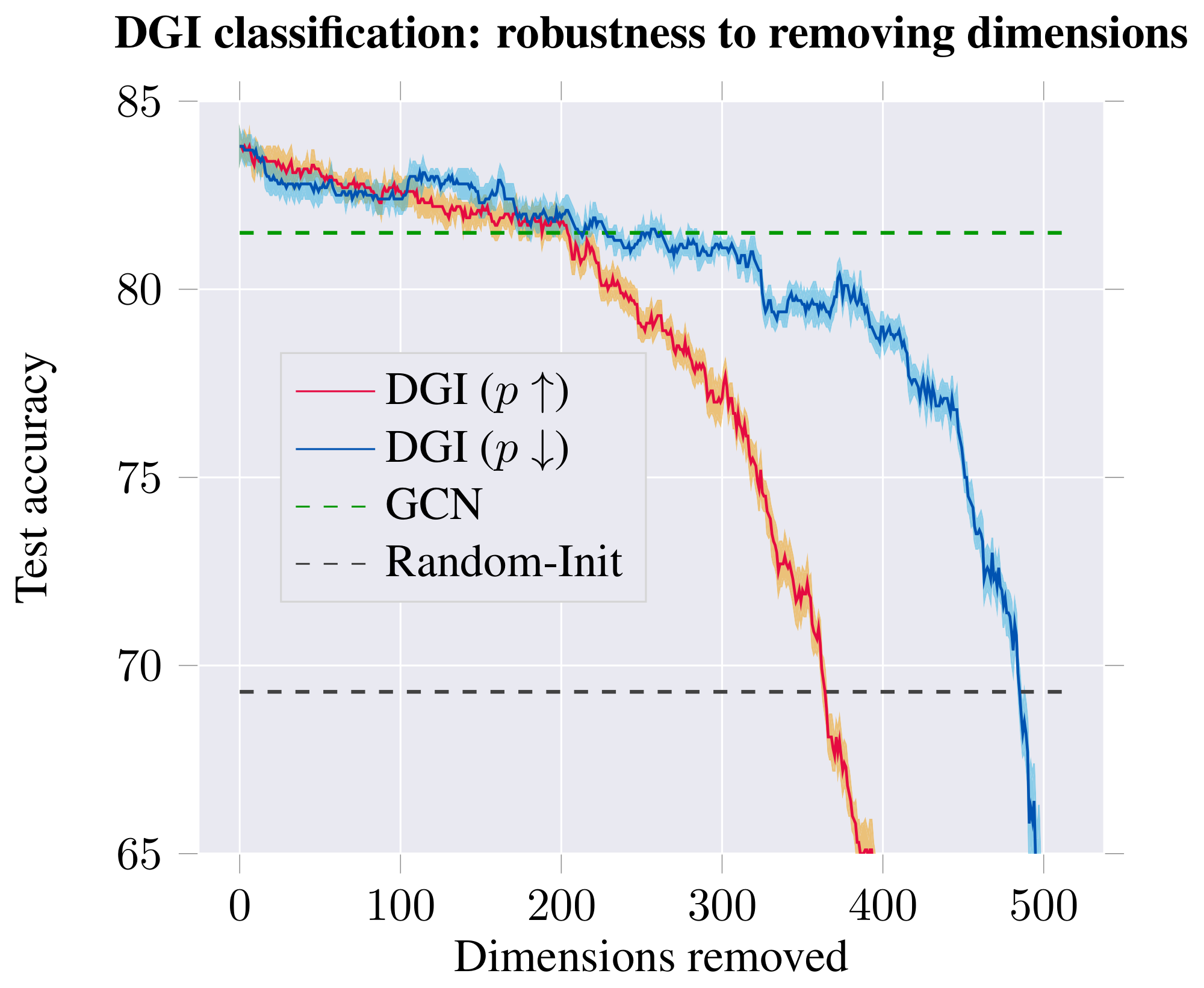
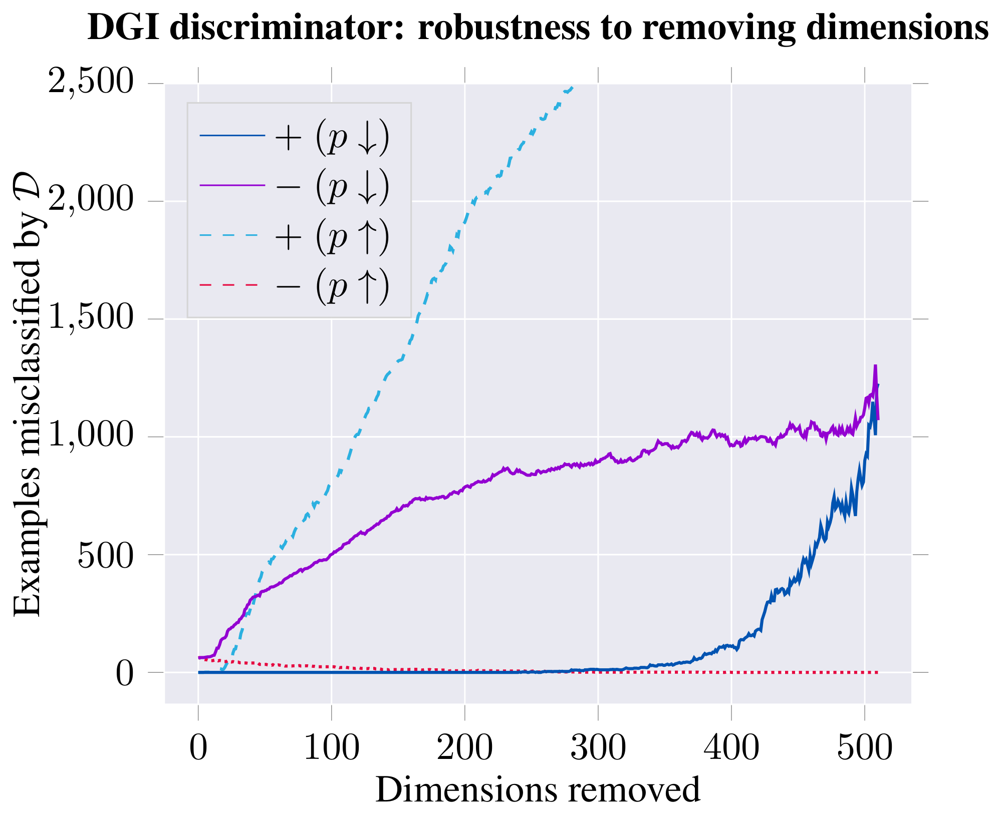
Figure 6: Classification performance (in terms of test accuracy of logistic regression; left) and discriminator performance (in terms of number of poorly discriminated positive/negative examples; right) on the learnt DGI embeddings, after removing a certain number of dimensions from the embedding—either starting with most distinguishing ($p\uparrow$) or least distinguishing ($p\downarrow$). ::::

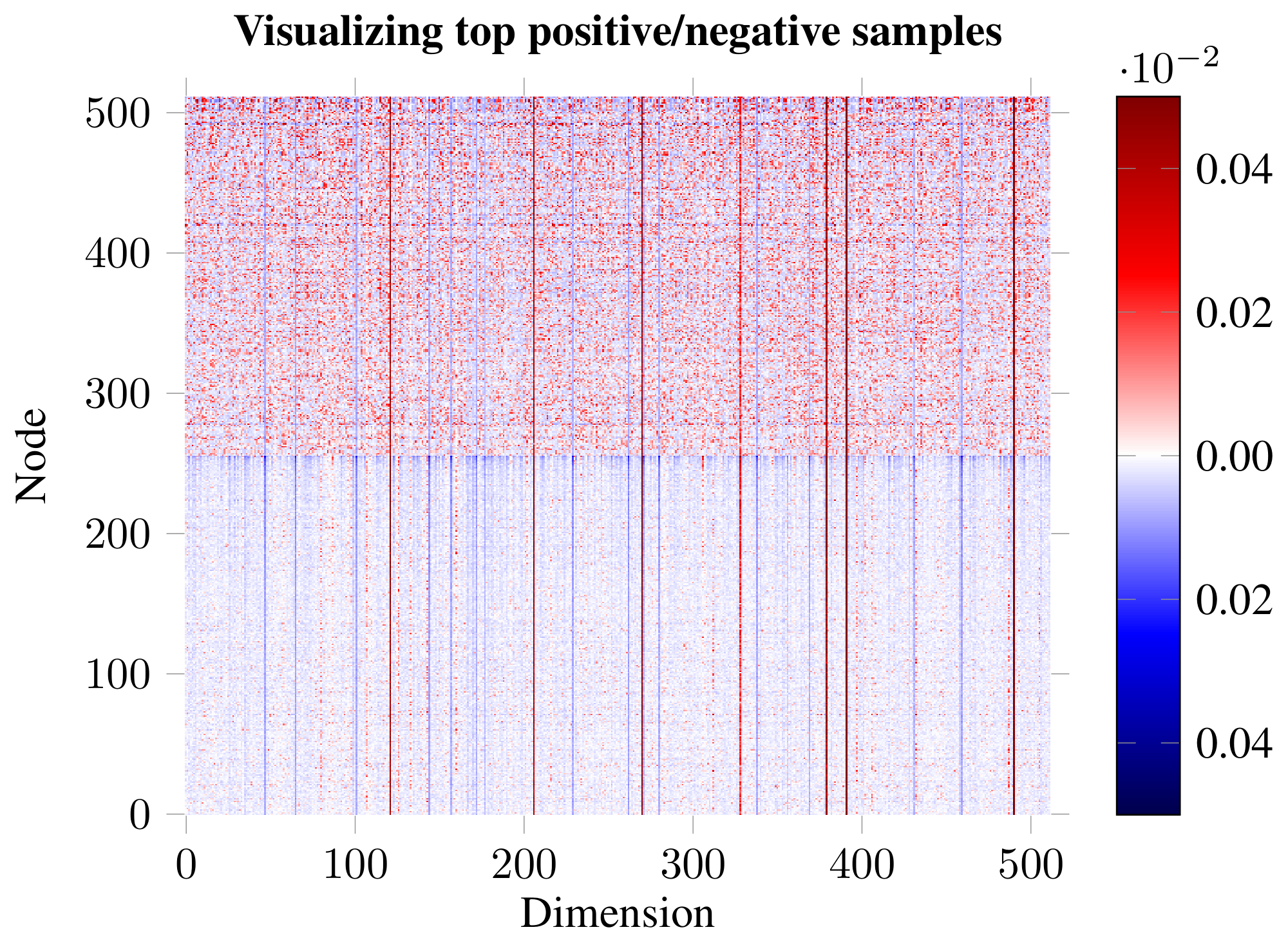
Impact and role of embedding dimensions. Guided by the previous result, we have visualized the embeddings for the top-scoring positive and negative examples (Figure 5). The analysis revealed existence of distinct dimensions in which both the positive and negative examples are strongly biased. We hypothesize that, given the random shuffling, the average expected activation of a negative example is zero, and therefore strong biases are required to "push" the example down in the discriminator. The positive examples may then use the remaining dimensions to both counteract this bias and encode patch similarity. To substantiate this claim, we order the 512 dimensions based on how distinguishable the positive and negative examples are in them (using $p$-values obtained from a t-test as a proxy). We then remove these dimensions from the embedding, respecting this order—either starting from the most distinguishable ($p\uparrow$) or least distinguishable dimensions ($p\downarrow$)—monitoring how this affects both classification and discriminator performance (Figure 6). The observed trends largely support our hypothesis: if we start by removing the biased dimensions first ($p\downarrow$), the classification performance holds up for much longer (allowing us to remove over half of the embedding dimensions while remaining competitive to the supervised GCN), and the positive examples mostly remain correctly discriminated until well over half the dimensions are removed.

C. Robustness to Choice of Corruption Function

Here, we consider alternatives to our corruption function, $\mathcal{C}$, used to produce negative graphs. We generally find that, for the node classification task, DGI is stable and robust to different strategies. However, for learning graph features towards other kinds of tasks, the design of appropriate corruption strategies remains an area of open research.

Our corruption function described in Section 4.2 preserves the original adjacency matrix (${\bf \widetilde{A}} = {\bf A}$) but corrupts the features, $\bf \widetilde{X}$, via row-wise shuffling of ${\bf X}$. In this case, the negative graph is constrained to be isomorphic to the positive graph, which should not have to be mandatory. We can instead produce a negative graph by directly corrupting the adjacency matrix.

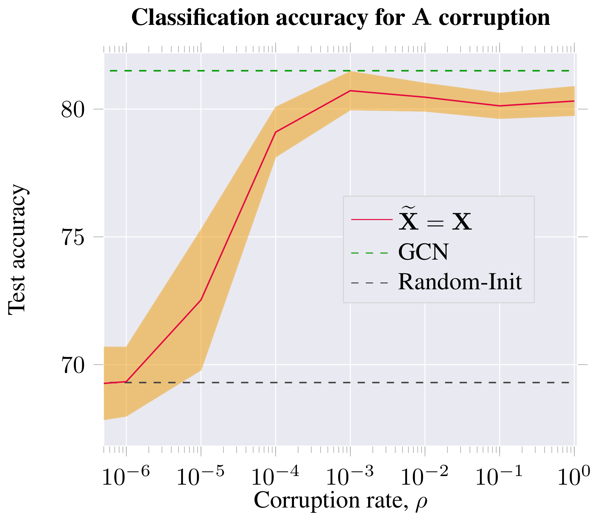
Therefore, we first consider an alternative corruption function $\mathcal{C}$ which preserves the features ($\bf \widetilde{X} = \bf X$) but instead adds or removes edges from the adjacency matrix ($\bf \widetilde{A} \neq \bf A$). This is done by sampling, i.i.d., a switch parameter ${\bf\Sigma}_{ij}$, which determines whether to corrupt the adjacency matrix at position $(i, j)$. Assuming a given corruption rate, $\rho$, we may define $\mathcal{C}$ as performing the following operations:

$ \begin{align} {\bf\Sigma}_{ij} &\sim \text{Bernoulli}(\rho)\ {\bf \widetilde{A}} &= {\bf A} \oplus {\bf\Sigma} \end{align} $

where $\oplus$ is the XOR (exclusive OR) operation.

This alternative strategy produces a negative graph with the same features, but different connectivity. Here, the corruption rate of $\rho=0$ corresponds to an unchanged adjacency matrix (i.e. the positive and negative graphs are identical in this case). In this regime, learning is impossible for the discriminator, and the performance of DGI is in line with a randomly initialized DGI model. At higher rates of noise, however, DGI produces competitive embeddings.

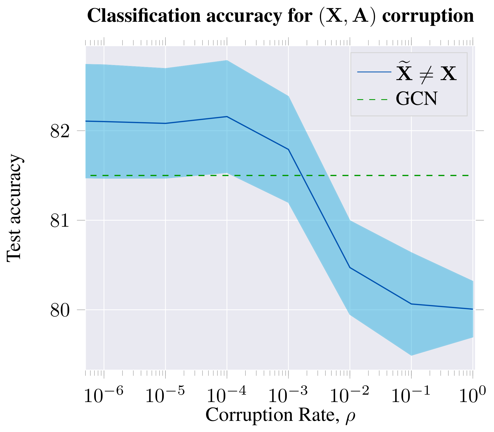
We also consider simultaneous feature shuffling ($\bf \widetilde{X} \neq \bf X$) and adjacency matrix perturbation (${\bf \widetilde{A}} \neq {\bf A}$), both as described before. We find that DGI still learns useful features under this compound corruption strategy—as expected, given that feature shuffling is already equivalent to an (isomorphic) adjacency matrix perturbation.

From both studies, we may observe that a certain lower bound on the positive graph perturbation rate is required to obtain competitive node embeddings for the classification task on Cora. Furthermore, the features learned for downstream node classification tasks are most powerful when the negative graph has similar levels of connectivity to the positive graph.

The classification performance peaks when the graph is perturbed to a reasonably high level, but remains sparse; i.e. the mixing between the separate 1-step patches is not substantial, and therefore the pool of negative examples is still diverse enough. Classification performance is impacted only marginally at higher rates of corruption—corresponding to dense negative graphs, and thus a less rich negative example pool—but still considerably outperforming the unsupervised baselines we have considered. This could be seen as further motivation for relying solely on feature shuffling, without adjacency perturbations—given that feature shuffling is a trivial way to guarantee a diverse set of negative examples, without incurring significant computational costs per epoch.

The results of this study are visualized in Figure 7 and Figure 8.

References

Section Summary: This references section lists about 29 academic papers and preprints from 2003 to 2018, focusing on advancements in machine learning for graph-based data, such as social networks or molecular structures that don't fit traditional grid-like patterns. Key topics include techniques for embedding nodes into lower-dimensional spaces for easier analysis, graph convolutional networks that process relationships like neurons in the brain, and methods like attention mechanisms or contrastive learning to improve predictions and representations. These works, from researchers at institutions like Google, Stanford, and universities, build foundational tools for applications in recommendation systems, chemistry, and natural language processing.

[1] Michael M Bronstein, Joan Bruna, Yann LeCun, Arthur Szlam, and Pierre Vandergheynst. Geometric deep learning: going beyond euclidean data. IEEE Signal Processing Magazine, 34(4):18–42, 2017.

[2] William L Hamilton, Rex Ying, and Jure Leskovec. Representation learning on graphs: Methods and applications. arXiv preprint arXiv:1709.05584, 2017b.

[3] Peter W Battaglia, Jessica B Hamrick, Victor Bapst, Alvaro Sanchez-Gonzalez, Vinicius Zambaldi, Mateusz Malinowski, Andrea Tacchetti, David Raposo, Adam Santoro, Ryan Faulkner, et al. Relational inductive biases, deep learning, and graph networks. arXiv preprint arXiv:1806.01261, 2018.

[4] Thomas N Kipf and Max Welling. Semi-supervised classification with graph convolutional networks. arXiv preprint arXiv:1609.02907, 2016a.

[5] Justin Gilmer, Samuel S Schoenholz, Patrick F Riley, Oriol Vinyals, and George E Dahl. Neural message passing for quantum chemistry. arXiv preprint arXiv:1704.01212, 2017.

[6] Petar Veličković, Guillem Cucurull, Arantxa Casanova, Adriana Romero, Pietro Liò, and Yoshua Bengio. Graph Attention Networks. International Conference on Learning Representations, 2018. URL https://openreview.net/forum?id=rJXMpikCZ.

[7] Aditya Grover and Jure Leskovec. node2vec: Scalable feature learning for networks. In Proceedings of the 22nd ACM SIGKDD international conference on Knowledge discovery and data mining, pp.\ 855–864. ACM, 2016.

[8] Bryan Perozzi, Rami Al-Rfou, and Steven Skiena. Deepwalk: Online learning of social representations. In Proceedings of the 20th ACM SIGKDD international conference on Knowledge discovery and data mining, pp.\ 701–710. ACM, 2014.

[9] Jian Tang, Meng Qu, Mingzhe Wang, Ming Zhang, Jun Yan, and Qiaozhu Mei. Line: Large-scale information network embedding. In Proceedings of the 24th International Conference on World Wide Web, pp.\ 1067–1077. International World Wide Web Conferences Steering Committee, 2015.

[10] Will Hamilton, Zhitao Ying, and Jure Leskovec. Inductive representation learning on large graphs. In Advances in Neural Information Processing Systems, pp.\ 1024–1034, 2017a.

[11] Thomas N Kipf and Max Welling. Variational graph auto-encoders. arXiv preprint arXiv:1611.07308, 2016b.

[12] Alberto Garcia Duran and Mathias Niepert. Learning graph representations with embedding propagation. In Advances in Neural Information Processing Systems, pp.\ 5119–5130, 2017.

[13] Glen Jeh and Jennifer Widom. Scaling personalized web search. In Proceedings of the 12th International Conference on the World Wide Web, pp.\ 271–279. Acm, 2003.

[14] Leonardo FR Ribeiro, Pedro HP Saverese, and Daniel R Figueiredo. struc2vec: Learning node representations from structural identity. In Proceedings of the 23rd ACM SIGKDD International Conference on Knowledge Discovery and Data Mining, pp.\ 385–394. ACM, 2017.

[15] Ishmael Belghazi, Aristide Baratin, Sai Rajeswar, Sherjil Ozair, Yoshua Bengio, Aaron Courville, and R Devon Hjelm. Mine: mutual information neural estimation. arXiv preprint arXiv:1801.04062, ICML'2018, 2018.

[16] R Devon Hjelm, Alex Fedorov, Samuel Lavoie-Marchildon, Karan Grewal, Adam Trischler, and Yoshua Bengio. Learning deep representations by mutual information estimation and maximization. arXiv preprint arXiv:1808.06670, 2018.

[17] Ronan Collobert and Jason Weston. A unified architecture for natural language processing: Deep neural networks with multitask learning. In Proceedings of the 25th international conference on Machine learning, pp.\ 160–167. ACM, 2008.

[18] Andriy Mnih and Koray Kavukcuoglu. Learning word embeddings efficiently with noise-contrastive estimation. In Advances in neural information processing systems, pp.\ 2265–2273, 2013.

[19] Tomas Mikolov, Ilya Sutskever, Kai Chen, Greg S Corrado, and Jeff Dean. Distributed representations of words and phrases and their compositionality. In Advances in neural information processing systems, pp.\ 3111–3119, 2013.

[20] Aleksandar Bojchevski and Stephan Günnemann. Deep gaussian embedding of graphs: Unsupervised inductive learning via ranking. In International Conference on Learning Representations, 2018. URL https://openreview.net/forum?id=r1ZdKJ-0W.

[21] Rex Ying, Ruining He, Kaifeng Chen, Pong Eksombatchai, William L Hamilton, and Jure Leskovec. Graph convolutional neural networks for web-scale recommender systems. arXiv preprint arXiv:1806.01973, 2018a.

[22] Avishek Bose, Huan Ling, and Yanshuai Cao. Adversarial contrastive estimation. In ACL, 2018.

[23] Aaron van den Oord, Yazhe Li, and Oriol Vinyals. Representation learning with contrastive predictive coding. arXiv preprint arXiv:1807.03748, 2018.

[24] Michael Gutmann and Aapo Hyvärinen. Noise-contrastive estimation: A new estimation principle for unnormalized statistical models. In Proceedings of the Thirteenth International Conference on Artificial Intelligence and Statistics, pp.\ 297–304, 2010.

[25] Daixin Wang, Peng Cui, and Wenwu Zhu. Structural deep network embedding. In Proceedings of the 22nd ACM SIGKDD international conference on Knowledge discovery and data mining, pp.\ 1225–1234. ACM, 2016.

[26] Xiao Wang, Peng Cui, Jing Wang, Jian Pei, Wenwu Zhu, and Shiqiang Yang. Community preserving network embedding. In AAAI, pp.\ 203–209, 2017.

[27] Ian Goodfellow, Jean Pouget-Abadie, Mehdi Mirza, Bing Xu, David Warde-Farley, Sherjil Ozair, Aaron Courville, and Yoshua Bengio. Generative adversarial nets. In Advances in neural information processing systems, pp.\ 2672–2680, 2014.

[28] Sebastian Nowozin, Botond Cseke, and Ryota Tomioka. f-gan: Training generative neural samplers using variational divergence minimization. In Advances in Neural Information Processing Systems, pp.\ 271–279, 2016.

[29] Claire Donnat, Marinka Zitnik, David Hallac, and Jure Leskovec. Learning structural node embeddings via diffusion wavelets. In International ACM Conference on Knowledge Discovery and Data Mining (KDD), volume 24, 2018.

[30] Prithviraj Sen, Galileo Namata, Mustafa Bilgic, Lise Getoor, Brian Galligher, and Tina Eliassi-Rad. Collective classification in network data. AI magazine, 29(3):93, 2008.

[31] Marinka Zitnik and Jure Leskovec. Predicting multicellular function through multi-layer tissue networks. Bioinformatics, 33(14):i190–i198, 2017.

[32] Kaiming He, Xiangyu Zhang, Shaoqing Ren, and Jian Sun. Delving deep into rectifiers: Surpassing human-level performance on imagenet classification. In Proceedings of the IEEE international conference on computer vision, pp.\ 1026–1034, 2015.

[33] Kaiming He, Xiangyu Zhang, Shaoqing Ren, and Jian Sun. Deep residual learning for image recognition. In Proceedings of the IEEE conference on computer vision and pattern recognition, pp.\ 770–778, 2016.

[34] Gao Huang, Zhuang Liu, Laurens Van Der Maaten, and Kilian Q Weinberger. Densely connected convolutional networks. In CVPR, volume 1, pp.\ 3, 2017.

[35] Nitish Srivastava, Geoffrey E Hinton, Alex Krizhevsky, Ilya Sutskever, and Ruslan Salakhutdinov. Dropout: a simple way to prevent neural networks from overfitting. Journal of machine learning research, 15(1):1929–1958, 2014.

[36] Oriol Vinyals, Samy Bengio, and Manjunath Kudlur. Order matters: Sequence to sequence for sets. arXiv preprint arXiv:1511.06391, 2015.

[37] Rex Ying, Jiaxuan You, Christopher Morris, Xiang Ren, William L Hamilton, and Jure Leskovec. Hierarchical graph representation learning with differentiable pooling. arXiv preprint arXiv:1806.08804, 2018b.

[38] Xavier Glorot and Yoshua Bengio. Understanding the difficulty of training deep feedforward neural networks. In Proceedings of the Thirteenth International Conference on Artificial Intelligence and Statistics, pp.\ 249–256, 2010.

[39] Diederik Kingma and Jimmy Ba. Adam: A method for stochastic optimization. arXiv preprint arXiv:1412.6980, 2014.

[40] Xiaojin Zhu, Zoubin Ghahramani, and John D Lafferty. Semi-supervised learning using gaussian fields and harmonic functions. In Proceedings of the 20th International conference on Machine learning (ICML-03), pp.\ 912–919, 2003.

[41] Zhilin Yang, William W Cohen, and Ruslan Salakhutdinov. Revisiting semi-supervised learning with graph embeddings. arXiv preprint arXiv:1603.08861, 2016.

[42] Jie Chen, Tengfei Ma, and Cao Xiao. Fastgcn: fast learning with graph convolutional networks via importance sampling. arXiv preprint arXiv:1801.10247, 2018.

[43] Jiani Zhang, Xingjian Shi, Junyuan Xie, Hao Ma, Irwin King, and Dit-Yan Yeung. Gaan: Gated attention networks for learning on large and spatiotemporal graphs. arXiv preprint arXiv:1803.07294, 2018.

[44] Ming Ding, Jie Tang, and Jie Zhang. Semi-supervised learning on graphs with generative adversarial nets. arXiv preprint arXiv:1809.00130, 2018.

[45] Boris Weisfeiler and AA Lehman. A reduction of a graph to a canonical form and an algebra arising during this reduction. Nauchno-Technicheskaya Informatsia, 2(9):12–16, 1968.

[46] Laurens van der Maaten and Geoffrey Hinton. Visualizing data using t-sne. Journal of Machine Learning Research, 9(Nov):2579–2605, 2008.

[47] Peter J Rousseeuw. Silhouettes: a graphical aid to the interpretation and validation of cluster analysis. Journal of computational and applied mathematics, 20:53–65, 1987.

[48] Adam Paszke, Sam Gross, Soumith Chintala, Gregory Chanan, Edward Yang, Zachary DeVito, Zeming Lin, Alban Desmaison, Luca Antiga, and Adam Lerer. Automatic differentiation in pytorch. In NIPS-W, 2017.

[49] Jeffrey Pennington, Richard Socher, and Christopher Manning. Glove: Global vectors for word representation. In Proceedings of the 2014 conference on empirical methods in natural language processing (EMNLP), pp.\ 1532–1543, 2014.

[50] Aravind Subramanian, Pablo Tamayo, Vamsi K Mootha, Sayan Mukherjee, Benjamin L Ebert, Michael A Gillette, Amanda Paulovich, Scott L Pomeroy, Todd R Golub, Eric S Lander, et al. Gene set enrichment analysis: a knowledge-based approach for interpreting genome-wide expression profiles. Proceedings of the National Academy of Sciences, 102(43):15545–15550, 2005.