A Reductions Approach to Fair Classification

Alekh Agarwal$^{1}$
Microsoft Research, New York

Alina Beygelzimer$^{2}$
Yahoo! Research, New York

Miroslav Dudík$^{1}$
Microsoft Research, New York

John Langford$^{1}$
Microsoft Research, New York

Hanna Wallach$^{1}$
Microsoft Research, New York

Abstract

We present a systematic approach for achieving fairness in a binary classification setting. While we focus on two well-known quantitative definitions of fairness, our approach encompasses many other previously studied definitions as special cases. The key idea is to reduce fair classification to a sequence of cost-sensitive classification problems, whose solutions yield a randomized classifier with the lowest (empirical) error subject to the desired constraints. We introduce two reductions that work for any representation of the cost-sensitive classifier and compare favorably to prior baselines on a variety of data sets, while overcoming several of their disadvantages.

$^{1}$ Microsoft Research, New York $^{2}$ Yahoo! Research, New York.
Correspondence to: A. Agarwal [email protected], A. Beygelzimer [email protected], M. Dudík [email protected], J. Langford [email protected], H. Wallach [email protected].
Proceedings of the 35$^{th}$ International Conference on Machine Learning, Stockholm, Sweden, PMLR 80, 2018. Copyright 2018 by the author(s).

Executive Summary: The document introduces a general reductions-based framework for training accurate binary classifiers subject to quantitative fairness constraints. The work responds to growing concerns that standard machine-learning systems can produce decisions with unintended disparate impact on protected groups such as race or sex. Existing methods either restrict the choice of base learner, enforce only approximate or weaker notions of fairness, require test-time access to the protected attribute, or fail to achieve the best attainable accuracy-fairness trade-off.

The authors set out to produce the lowest-error classifier (possibly randomized) that satisfies any fairness definition expressible as linear inequalities on conditional moments—most notably demographic parity and equalized odds—while treating the underlying classification algorithm as a black box. The key technical move is to rewrite the resulting constrained optimization problem as a saddle-point problem whose solution can be found by repeatedly solving ordinary cost-sensitive classification tasks. An exponentiated-gradient algorithm on the dual variables yields a sequence of base classifiers whose convex combination meets the fairness constraints up to a small, controllable violation. Finite-sample guarantees are derived that bound both excess error and constraint violation in terms of Rademacher complexity; the number of iterations required remains modest when the number of constraints is small.

Across four real-world data sets (adult income, COMPAS recidivism, law-school bar passage, and Dutch census), the resulting randomized classifiers achieve lower or statistically indistinguishable error for any given level of fairness violation compared with three established baselines: score-based post-processing, reweighting, and relabeling. The method works with logistic regression or gradient-boosted trees, supports both binary and non-binary protected attributes, needs the protected attribute only at training time, and can trace out the full accuracy–fairness frontier simply by varying a slack parameter. When the protected attribute is binary, an even simpler one-dimensional grid search over Lagrange multipliers recovers essentially the same performance.

These results matter for organizations that must deploy accurate models while satisfying legal or ethical requirements. Because the approach is modular and comes with explicit error and fairness guarantees, practitioners can enforce a chosen fairness definition without sacrificing more accuracy than necessary and without locking themselves into a particular model family. The experiments also show that earlier “wrapper” techniques often leave residual unfairness or incur larger accuracy penalties, underscoring the value of an optimization-based reduction.

The authors recommend that practitioners adopt the exponentiated-gradient procedure (or the cheaper grid search when feasible) whenever training-time access to the protected attribute is available and a single quantitative fairness definition is desired. When multiple, possibly conflicting fairness criteria must be satisfied simultaneously, or when the protected attribute is unavailable at training time, additional algorithmic work is required. In all cases, the framework’s statistical guarantees depend on sufficient sample sizes within each protected group; therefore, data-collection or stratification decisions should be revisited before deployment if any group is very small. Overall the empirical and theoretical evidence supports replacing prior ad-hoc methods with the reductions approach for most practical fairness-constrained classification tasks.

1. Introduction

Section Summary: Recent years have seen growing public concern about machine learning systems that unintentionally discriminate against protected groups when making decisions such as allocating jobs or loans. This paper focuses on binary classification subject to fairness constraints defined by a sensitive attribute like race or sex, and it introduces a general method that treats any existing classifier as a black box while reducing the constrained problem to a sequence of cost-sensitive classification tasks. The resulting randomized classifier achieves the lowest possible error among all fair solutions and avoids drawbacks of prior approaches, such as reliance on strong assumptions, limited flexibility, or the need for protected-attribute data at test time.

Over the past few years, the media have paid considerable attention to machine learning systems and their ability to inadvertently discriminate against minorities, historically disadvantaged populations, and other protected groups when allocating resources (e.g., loans) or opportunities (e.g., jobs). In response to this scrutiny—and driven by ongoing debates and collaborations with lawyers, policy-makers, social scientists, and others (e.g., [1])—machine learning researchers have begun to turn their attention to the topic of "fairness in machine learning, " and, in particular, to the design of fair classification and regression algorithms.

In this paper we study the task of binary classification subject to fairness constraints with respect to a pre-defined protected attribute, such as race or sex. Previous work in this area can be divided into two broad groups of approaches.

The first group of approaches incorporate specific quantitative definitions of fairness into existing machine learning methods, often by relaxing the desired definitions of fairness, and only enforcing weaker constraints, such as lack of correlation (e.g., [2, 3, 4, 5, 6]). The resulting fairness guarantees typically only hold under strong distributional assumptions, and the approaches are tied to specific families of classifiers, such as SVMs.

The second group of approaches eliminate the restriction to specific classifier families and treat the underlying classification method as a "black box, " while implementing a wrapper that either works by pre-processing the data or post-processing the classifier's predictions (e.g., [7, 8, 9, 10]). Existing pre-processing approaches are specific to particular definitions of fairness and typically seek to come up with a single transformed data set that will work across all learning algorithms, which, in practice, leads to classifiers that still exhibit substantial unfairness (see our evaluation in Section 4). In contrast, post-processing allows a wider range of fairness definitions and results in provable fairness guarantees. However, it is not guaranteed to find the most accurate fair classifier, and requires test-time access to the protected attribute, which might not be available.

We present a general-purpose approach that has the key advantage of this second group of approaches—i.e., the underlying classification method is treated as a black box—but without the noted disadvantages. Our approach encompasses a wide range of fairness definitions, is guaranteed to yield the most accurate fair classifier, and does not require test-time access to the protected attribute. Specifically, our approach allows any definition of fairness that can be formalized via linear inequalities on conditional moments, such as demographic parity or equalized odds (see Section 2.1). We show how binary classification subject to these constraints can be reduced to a sequence of cost-sensitive classification problems. We require only black-box access to a cost-sensitive classification algorithm, which does not need to have any knowledge of the desired definition of fairness or protected attribute. We show that the solutions to our sequence of cost-sensitive classification problems yield a randomized classifier with the lowest (empirical) error subject to the desired fairness constraints.

[11] and [12] begin with a similar goal to ours, but they analyze the Bayes optimal classifier under fairness constraints in the limit of infinite data. In contrast, our focus is algorithmic, our approach applies to any classifier family, and we obtain finite-sample guarantees. [13] also begin with a similar goal to ours. Their approach partitions the training examples into subsets according to protected attribute values and then leverages transfer learning to jointly learn from these separate data sets. Our approach avoids partitioning the data and assumes access only to a classification algorithm rather than a transfer learning algorithm.

A preliminary version of this paper appeared at the FAT/ML workshop ([14]), and led to extensions with more general optimization objectives ([15]) and combinatorial protected attributes ([16]).

In the next section, we formalize our problem. While we focus on two well-known quantitative definitions of fairness, our approach also encompasses many other previously studied definitions of fairness as special cases. In Section 3, we describe our reductions approach to fair classification and its guarantees in detail. The experimental study in Section 4 shows that our reductions compare favorably to three baselines, while overcoming some of their disadvantages and also offering the flexibility of picking a suitable accuracy–fairness tradeoff. Our results demonstrate the utility of having a general-purpose approach for combining machine learning methods and quantitative fairness definitions.

2. Problem Formulation

Section Summary: In a binary classification task, each data point consists of features X—which may include or correlate with a protected attribute A such as race—along with a binary label Y such as loan default. The aim is to train a classifier from a given family that predicts Y accurately while obeying formal fairness rules that limit dependence between the predictions and A. The section introduces two standard fairness criteria, demographic parity and equalized odds, and shows that both can be written as linear inequality constraints on certain conditional expectations involving the classifier.

We consider a binary classification setting where the training examples consist of triples $(X, A, Y)$, where $X\in \mathcal{X}$ is a feature vector, $A \in \mathcal{A}$ is a protected attribute, and $Y \in {0, 1}$ is a label. The feature vector $X$ can either contain the protected attribute $A$ as one of the features or contain other features that are arbitrarily indicative of $A$. For example, if the classification task is to predict whether or not someone will default on a loan, each training example might correspond to a person, where $X$ represents their demographics, income level, past payment history, and loan amount; $A$ represents their race; and $Y$ represents whether or not they defaulted on that loan. Note that $X$ might contain their race as one of the features or, for example, contain their zipcode—a feature that is often correlated with race. Our goal is to learn an accurate classifier $h: \mathcal{X}\to {0, 1}$ from some set (i.e., family) of classifiers $\mathcal{H}$, such as linear threshold rules, decision trees, or neural nets, while satisfying some definition of fairness. Note that the classifiers in $\mathcal{H}$ do not explicitly depend on $A$.

2.1 Fairness Definitions

We focus on two well-known quantitative definitions of fairness that have been considered in previous work on fair classification; however, our approach also encompasses many other previously studied definitions of fairness as special cases, as we explain at the end of this section.

The first definition—demographic (or statistical) parity—can be thought of as a stronger version of the US Equal Employment Opportunity Commission's "four-fifths rule, " which requires that the "selection rate for any race, sex, or ethnic group [must be at least] four-fifths (4/5) (or eighty percent) of the rate for the group with the highest rate."[^1]

[^1]: See the Uniform Guidelines on Employment Selection Procedures, 29 C.F.R. § 1607.4(D) (2015).

########## {caption="Definition 1: Demographic parity—DP"}

A classifier $h$ satisfies demographic parity under a distribution over $(X, A, Y)$ if its prediction $h(X)$ is statistically independent of the protected attribute $A$ —that is, if $\mathbb{P}[{h(X)=\hat{y}} \mathbin{\vert} A=a] = \mathbb{P}[h(X)=\hat{y}]$ for all $a$, $\hat{y}$. Because $\hat{y}\in{0, 1}$, this is equivalent to ${\mathbb{E}[h(X)\mathbin{\vert} A=a]}= \mathbb{E}[h(X)]$ for all $a$.

The second definition—equalized odds—was recently proposed by [9] to remedy two previously noted flaws with demographic parity ([17]). First, demographic parity permits a classifier which accurately classifies data points with one value ${A=a}$, such as the value $a$ with the most data, but makes random predictions for data points with ${A\ne a}$ as long as the probabilities of ${h(X)=1}$ match. Second, demographic parity rules out perfect classifiers whenever $Y$ is correlated with $A$. In contrast, equalized odds suffers from neither of these flaws.

########## {caption="Definition 2: Equalized odds—EO"}

A classifier $h$ satisfies equalized odds under a distribution over $(X, A, Y)$ if its prediction $h(X)$ is conditionally independent of the protected attribute $A$ given the label $Y$ —that is, if $\mathbb{P}[{h(X)=\hat{y}} \mathbin{\vert} A=a, Y=y] = \mathbb{P}[{h(X)=\hat{y}} \mathbin{\vert} Y=y]$ for all $a$, $y$, and $\hat{y}$. Because $\hat{y}\in{0, 1}$, this is equivalent to $\mathbb{E}[h(X)\mathbin{\vert} A=a, Y=y]= \mathbb{E}[h(X)\mathbin{\vert} Y=y]$ for all $a$, $y$.

We now show how each definition can be viewed as a special case of a general set of linear constraints of the form

$ \mathbf{M} \boldsymbol{\mu}(h) \leq {\mathbf{c}},\tag{1} $

where matrix $\mathbf{M} \in \mathbb{R}^{|\mathcal{K}| \times |\mathcal{J}|}$ and vector ${\mathbf{c}}\in \mathbb{R}^{|\mathcal{K}|}$ describe the linear constraints, each indexed by $k\in \mathcal{K}$, and $\boldsymbol{\mu}(h) \in \mathbb{R}^{|\mathcal{J}|}$ is a vector of conditional moments of the form

$ \mu_j(h) = \mathbb{E}\bigl[, g_j(X, A, Y, h(X)), \mathbin{\bigm\vert} , \mathcal{E}_j, \bigr] \quad \text{for }j \in \mathcal{J}, $

where $g_j : {\mathcal{X}\times \mathcal{A}\times{0, 1}\times{0, 1}} \to [0, 1]$ and $\mathcal{E}_j$ is an event defined with respect to $(X, A, Y)$. Crucially, $g_j$ depends on $h$, while $\mathcal{E}_j$ cannot depend on $h$ in any way.

########## {caption="Example: DP"}

In a binary classification setting, demographic parity can be expressed as a set of $|\mathcal{A}|$ equality constraints, each of the form $\mathbb{E}[h(X) \mathbin{\vert} A = a] = \mathbb{E}[h(X)]$. Letting $\mathcal{J} = \mathcal{A} \cup { \star }$, $g_j(X, A, Y, h(X)) = h(X)$ for all $j$, $\mathcal{E}{a} = {A = a}$, and $\mathcal{E}{\star} = {\textit{True}}$, where ${\textit{True}}$ refers to the event encompassing all points in the sample space, each equality constraint can be expressed as $\mu_a(h) = \mu_{\star}(h)$.[^2] Finally, because each such constraint can be equivalently expressed as a pair of inequality constraints of the form

[^2]: Note that $\mu_\star(h) = \mathbb{E}[h(X) , |, \textit{True}] = \mathbb{E}[h(X)]$.

$ \begin{aligned} \mu_a(h) - \mu_{\star}(h) &\leq 0\ -\mu_a(h) + \mu_{\star}(h) &\leq 0, \end{aligned} $

demographic parity can be expressed as equation 1, where $\mathcal{K} = \mathcal{A} \times {+, -}$, $M_{(a, +), a'} = \mathbf{1}{a' = a}$, $M_{(a, +), \star}=-1$, $M_{(a, -), a'} = -\mathbf{1}{a' = a}$, $M_{(a, -), \star} = 1$, and ${\mathbf{c}} = \boldsymbol{0}$. Expressing each equality constraint as a pair of inequality constraints allows us to control the extent to which each constraint is enforced by positing $c_k>0$ for some (or all) $k$.

########## {caption="Example: EO"}

In a binary classification setting, equalized odds can be expressed as a set of $2, \lvert\mathcal{A}\rvert$ equality constraints, each of the form $\mathbb{E}[h(X) \mathbin{\vert} A=a, {Y!=y}] = \mathbb{E}[h(X)\mathbin{\vert} {Y!=y}]$. Letting $\mathcal{J} = (\mathcal{A}\cup{\star})\times{0, 1}$, $g_j(X, A, Y, h(X)) = h(X)$ for all $j$, $\mathcal{E}{(a, y)} = {A=a, {Y!=y}}$, and $\mathcal{E}{(\star, y)} = {Y!=y}$, each equality constraint can be equivalently expressed as

$ \begin{aligned} \mu_{(a, y)}(h) - \mu_{(\star, y)}(h) &\leq 0\ -\mu_{(a, y)}(h) + \mu_{(\star, y)}(h) &\leq 0. \end{aligned} $

As a result, equalized odds can be expressed as equation 1, where $\mathcal{K} = {\mathcal{A} \times \mathcal{Y} \times {+, -}}$, $M_{(a, y, +), (a', y')} = \mathbf{1}{a'!!=!a, , y'!!=!y}$, $M_{(a, y, +), (\star, y')}=-1$, $M_{(a, y, -), (a', y')} = -\mathbf{1}{a'!!=!a, , y'!!=!y}$, $M_{(a, y, -), (\star, y')} = 1$, and ${\mathbf{c}}= \mathbf{0}$. Again, we can posit $c_k>0$ for some (or all) $k$ to allow small violations of some (or all) of the constraints.

Although we omit the details, we note that many other previously studied definitions of fairness can also be expressed as equation 1. For example, equality of opportunity [9] (also known as balance for the positive class; [18]), balance for the negative class [18], error-rate balance [19], overall accuracy equality [20], and treatment equality [20] can all be expressed as equation 1; in contrast, calibration [18] and predictive parity [19] cannot because to do so would require the event $\mathcal{E}_j$ to depend on $h$. We note that our approach can also be used to satisfy multiple definitions of fairness, though if these definitions are mutually contradictory, e.g., as described by [18], then our guarantees become vacuous.

2.2 Fair Classification

In a standard (binary) classification setting, the goal is to learn the classifier $h\in \mathcal{H}$ with the minimum classification error: $\textup{err}(h)\coloneqq \mathbb{P}[h(X) \neq Y]$. However, because our goal is to learn the most accurate classifier while satisfying fairness constraints, as formalized above, we instead seek to find the solution to the constrained optimization problem[^3]

[^3]: We consider misclassification error for concreteness, but all the results in this paper apply to any error of the form $\textup{err}(h) = \mathbb{E}[g_\textup{err}(X, A, Y, h(X))]$, where $g_\textup{err}(\cdot, \cdot, \cdot, \cdot)\in[0, 1]$.

$ \min_{h \in \mathcal{H}} err(h) \quad \text{subject to} \quad \mathbf{M} \boldsymbol{\mu}(h) \leq {\mathbf{c}}. $

Furthermore, rather than just considering classifiers in the set $\mathcal{H}$, we can enlarge the space of possible classifiers by considering randomized classifiers that can be obtained via a distribution over $\mathcal{H}$. By considering randomized classifiers, we can achieve better accuracy–fairness tradeoffs than would otherwise be possible. A randomized classifier $Q$ makes a prediction by first sampling a classifier $h \in \mathcal{H}$ from $Q$ and then using $h$ to make the prediction. The resulting classification error is $\textup{err}(Q)=\sum_{h \in \mathcal{H}} Q(h), \textup{err}(h)$ and the conditional moments are $\boldsymbol{\mu}(Q) = \sum_{h \in \mathcal{H}} Q(h)\boldsymbol{\mu}(h)$ (see Appendix A for the derivation). Thus we seek to solve

$ \min_{Q \in \Delta} \textup{err}(Q) \quad \text{subject to} \quad \mathbf{M} \boldsymbol{\mu}(Q) \leq {\mathbf{c}},\tag{2} $

where $\Delta$ is the set of all distributions over $\mathcal{H}$.

In practice, we do not know the true distribution over $(X, A, Y)$ and only have access to a data set of training examples ${(X_i, A_i, Y_i)}_{i=1}^n$. We therefore replace $\textrm{err}(Q)$ and $\boldsymbol{\mu}(Q)$ in equation 2 with their empirical versions $\widehat{\textup{err}}(Q)$ and $\widehat{\boldsymbol{\mu}}(Q)$. Because of the sampling error in $\widehat{\boldsymbol{\mu}}(Q)$, we also allow errors in satisfying the constraints by setting $\widehat{c}_k = c_k + \varepsilon_k$ for all $k$, where $\varepsilon_k \geq 0$. After these modifications, we need to solve the empirical version of equation 2:

$ \min_{Q \in \Delta}\widehat{\textup{err}}(Q) \quad \text{subject to} \quad \mathbf{M} \widehat{\boldsymbol{\mu}}(Q) \leq \widehat{\mathbf{c}} .\tag{3} $

3. Reductions Approach

Section Summary: The reductions approach reformulates a constrained fair-classification task as a saddle-point problem by introducing Lagrange multipliers for the fairness constraints and then solving the resulting zero-sum game. One player selects a randomized classifier while the other adjusts the multipliers; the classifier player’s best response at each step is obtained by calling a cost-sensitive classification routine that encodes the current costs induced by the multipliers. Averaging the sequence of best-response classifiers produced by this iterative procedure yields a randomized predictor whose empirical error is minimal among all predictors that approximately satisfy the original fairness requirements.

We now show how the problem Equation 3 can be reduced to a sequence of cost-sensitive classification problems. We further show that the solutions to our sequence of cost-sensitive classification problems yield a randomized classifier with the lowest (empirical) error subject to the desired constraints.

3.1 Cost-sensitive Classification

We assume access to a cost-sensitive classification algorithm for the set $\mathcal{H}$. The input to such an algorithm is a data set of training examples ${(X_i, C_i^0, C_i^1)}_{i=1}^n$, where $C_i^0$ and $C_i^1$ denote the losses—costs in this setting—for predicting the labels $0$ or $1$, respectively, for $X_i$. The algorithm outputs

$ \operatorname{arg, min}{h \in \mathcal{H}} \sum{i=1}^n h(X_i), C_i^1 + (1-h(X_i)), C_i^0.\tag{4} $

This abstraction allows us to specify different costs for different training examples, which is essential for incorporating fairness constraints. Moreover, efficient cost-sensitive classification algorithms are readily available for several common classifier representations (e.g., [21, 22, 23]). In particular, equation 4 is equivalent to a weighted classification problem, where the input consists of labeled examples ${(X_i, Y_i, W_i)}{i=1}^n$ with $Y_i\in{0, 1}$ and $W_i\ge 0$, and the goal is to minimize the weighted classification error $\sum{i=1}^n W_i, \mathbf{1}{h(X_i)\ne Y_i}$. This is equivalent to equation 4 if we set $W_i=\lvert C_i^0-C_i^1\rvert$ and $Y_i= \mathbf{1}{C_i^0\ge C_i^1}$.

3.2 Reduction

To derive our fair classification algorithm, we rewrite equation 3 as a saddle point problem. We begin by introducing a Lagrange multiplier $\lambda_k\ge 0$ for each of the $| \mathcal{K}|$ constraints, summarized as $\boldsymbol{\lambda}\in \mathbb{R}_+^{| \mathcal{K}|}$, and form the Lagrangian

$ \begin{aligned} \notag L(Q, \boldsymbol{\lambda}) &= \widehat{\textup{err}}(Q) +\boldsymbol{\lambda}^{!\top}\bigl(\mathbf{M}\widehat{\boldsymbol{\mu}}(Q)-\widehat{\mathbf{c}}\bigr). \end{aligned} $

Thus, equation 3 is equivalent to

$ \min_{Q\in\Delta} \max_{;;; \boldsymbol{\lambda}\in \mathbb{R}_+^{| \mathcal{K}|};;;} L(Q, \boldsymbol{\lambda}).\tag{5} $

For computational and statistical reasons, we impose an additional constraint on the $\ell_1$ norm of $\boldsymbol{\lambda}$ and seek to simultaneously find the solution to the constrained version of Equation 5 as well as its dual, obtained by switching min and max:

$ \begin{aligned} \quad\text{(a)} \quad\text{(\textup{P})} \min_{Q\in\Delta\mathstrut} \max_{;;; \boldsymbol{\lambda}\in \mathbb{R}+^{| \mathcal{K}|}, , \lVert\boldsymbol{\lambda}\rVert_1\le B;;;} L(Q, \boldsymbol{\lambda}), \ \quad\text{(b)} \quad\text{(\textup{D})} \max{\boldsymbol{\lambda}\in \mathbb{R}+^{| \mathcal{K}|}, , \lVert\boldsymbol{\lambda}\rVert_1\le B} \min{;;;Q\in\Delta;;;\mathstrut} L(Q, \boldsymbol{\lambda}). \end{aligned}\tag{6} $

Because $L$ is linear in $Q$ and $\boldsymbol{\lambda}$ and the domains of $Q$ and $\boldsymbol{\lambda}$ are convex and compact, both problems have solutions (which we denote by $Q^\dagger$ and $\boldsymbol{\lambda}^\dagger$) and the minimum value of Equation 6a and the maximum value of Equation 6b are equal and coincide with $L(Q^\dagger, \boldsymbol{\lambda}^\dagger)$. Thus, $(Q^\dagger, \boldsymbol{\lambda}^\dagger)$ is the saddle point of $L$ (Corollary 37.6.2 and Lemma 36.2 of [24]).

We find the saddle point by using the standard scheme of [25], developed for the equivalent problem of solving for an equilibrium in a zero-sum game. From game-theoretic perspective, the saddle point can be viewed as an equilibrium of a game between two players: the $Q$-player choosing $Q$ and the $\boldsymbol{\lambda}$-player choosing $\boldsymbol{\lambda}$. The Lagrangian $L(Q, \boldsymbol{\lambda})$ specifies how much the $Q$-player has to pay to the $\boldsymbol{\lambda}$-player after they make their choices. At the saddle point, neither player wants to deviate from their choice.

Our algorithm finds an approximate equilibrium in which neither player can gain more than $\nu$ by changing their choice (where $\nu>0$ is an input to the algorithm). Such an approximate equilibrium corresponds to a $\nu$-approximate saddle point of the Lagrangian, which is a pair $(\widehat{Q}, \widehat{\boldsymbol{\lambda}})$, where

$ \begin{aligned} L(\widehat{Q}, \widehat{\boldsymbol{\lambda}}) &\le L(Q, \widehat{\boldsymbol{\lambda}})+\nu && \text{for all }Q\in\Delta, \ L(\widehat{Q}, \widehat{\boldsymbol{\lambda}}) &\ge L(\widehat{Q}, \boldsymbol{\lambda})-\nu && \text{for all }\boldsymbol{\lambda}\in \mathbb{R}_+^{| \mathcal{K}|}\text{, }\lVert\boldsymbol{\lambda}\rVert_1\le B. \end{aligned} $

We proceed iteratively by running a no-regret algorithm for the $\boldsymbol{\lambda}$-player, while executing the best response of the $Q$-player. Following [25], the average play of both players converges to the saddle point. We run the exponentiated gradient algorithm ([26]) for the $\boldsymbol{\lambda}$-player and terminate as soon as the suboptimality of the average play falls below the pre-specified accuracy $\nu$. The best response of the $Q$-player can always be chosen to put all of the mass on one of the candidate classifiers $h\in \mathcal{H}$, and can be implemented by a single call to a cost-sensitive classification algorithm for the set $\mathcal{H}$.

Algorithm 1 fully implements this scheme, except for the functions $\textsc{Best}_{\boldsymbol{\lambda}}$ and $\textsc{Best}_h$, which correspond to the best-response algorithms of the two players. (We need the best response of the $\boldsymbol{\lambda}$-player to evaluate whether the suboptimality of the current average play has fallen below $\nu$.) The two best response functions can be calculated as follows.

Input: training examples ((X(i),Y(i),A(i))) for i=1..n
fairness constraints specified by g(j), E(j), M, ĉ
bound B, accuracy nu, learning rate η
Set θ₁₌ 0∈ R(| K|)
**for** t=1, 2, … **do**
  Set λ(t), k = B
                (exp(θ(k)))/(1+∑ over k'∈ K exp(θ(k)'))
  for all k∈ K
  h(t)← BEST(h)(λ(t))
  Q̂(t←1/t∑) over t'=1..t h(t)',

            L̄← L(Q̂(t), BEST(λ)(Q̂(t)))
  λ̂(t←1/t∑) over t'=1..t λ(t)',

            L̲← L(BEST(h)(λ̂(t)), λ̂(t))
  nu(t)←max(L(Q̂(t), λ̂(t)-L̲),
                                    L̄-L(Q̂(t), λ̂(t))
                                  )
  **if** nu(t)≤nu **then**
    Return (Q̂(t), λ̂(t))
  **end if**
  Set θ(t+1)= θ(t+η)(Mμ̂(h(t))-ĉ)
**end for**

$\textsc{Best}_{\boldsymbol{\lambda}}(Q)$: the best response of the $\boldsymbol{\lambda}$-player.

The best response of the $\boldsymbol{\lambda}$-player for a given $Q$ is any maximizer of $L(Q, \boldsymbol{\lambda})$ over all valid $\boldsymbol{\lambda}$ s. In our setting, it can always be chosen to be either $\mathbf{0}$ or put all of the mass on the most violated constraint. Letting $\widehat{\boldsymbol{\gamma}}(Q)\coloneqq \mathbf{M}\widehat{\boldsymbol{\mu}}(Q)$ and letting $\mathbf{e}k$ denote the $k^\textrm{th}$ vector of the standard basis, $\textsc{Best}{\boldsymbol{\lambda}}(Q)$ returns

$ \begin{cases} \mathbf{0} &\text{if }\widehat{\boldsymbol{\gamma}}(Q)\le \widehat{\mathbf{c}}, \ B \mathbf{e}_{k^*} &\text{otherwise, where }k^*= \operatorname{arg, max}_k[\widehat{\gamma}_k(Q)-\widehat{c}_k]. \end{cases} $

$\textsc{Best}_h(\boldsymbol{\lambda})$: the best response of the $Q$-player.

Here, the best response minimizes $L(Q, \boldsymbol{\lambda})$ over all $Q$ s in the simplex. Because $L$ is linear in $Q$, the minimizer can always be chosen to put all of the mass on a single classifier $h$. We show how to obtain the classifier constituting the best response via a reduction to cost-sensitive classification. Letting $p_j\coloneqq \widehat{\mathbb{P}}[\mathcal{E}_j]$ be the empirical event probabilities, the Lagrangian for $Q$ which puts all of the mass on a single $h$ is then

$ \begin{aligned} & L(h, \boldsymbol{\lambda})

\widehat{\textup{err}}(h) +\boldsymbol{\lambda}^{!\top}\bigl(\mathbf{M}\widehat{\boldsymbol{\mu}}(h)-\widehat{\mathbf{c}}\bigr) \ &;

\widehat{\mathbb{E}}\bigl[\mathbf{1}{h(X)\ne Y}\bigr] -\boldsymbol{\lambda}^{!\top}\widehat{\mathbf{c}} +!\sum_{k, j} M_{k, j}\lambda_k \widehat{\mu}j(h) \ &;= -\boldsymbol{\lambda}^{!\top}\widehat{\mathbf{c}} +\widehat{\mathbb{E}}\bigl[\mathbf{1}{h(X)\ne Y}\bigr] \ &;\quad{} +!\sum{k, j} \frac{M_{k, j}\lambda_k}{p_j}\widehat{\mathbb{E}}\Bigl[g_j\bigl(X!, !A, !Y!, !h(X)\bigr), \mathbf{1}{(X!, !A, !Y)\in \mathcal{E}_j}\Bigr] . \end{aligned} $

Assuming a data set of training examples ${(X_i, A_i, Y_i)}{i=1}^n$, the minimization of $L(h, \boldsymbol{\lambda})$ over $h$ then corresponds to cost-sensitive classification on ${(X_i, C_i^0, C_i^1)}{i=1}^n$ with costs [^4]

[^4]: For general error, $\textup{err}(h) = \mathbb{E}[g_\textup{err}(X, A, Y, h(X))]$, the costs $C_i^0$ and $C_i^1$ contain, respectively, the terms $g_\textup{err}(X_i, A_i, Y_i, 0)$ and $g_\textup{err}(X_i, A_i, Y_i, 1)$ instead of $\mathbf{1}{Y_i\ne 0}$ and $\mathbf{1}{Y_i\ne 1}$.

$ \begin{aligned} C_i^0 &

\mathbf{1}{Y_i\ne 0} \ &;\quad{} +!\sum_{k, j} \frac{M_{k, j}\lambda_k}{p_j}g_j(X_i, !A_i, !Y_i, 0), \mathbf{1}{(X_i, !A_i, !Y_i)\in \mathcal{E}_j} \ C_i^1 &

\mathbf{1}{Y_i\ne 1} \ &;\quad{} +!\sum_{k, j} \frac{M_{k, j}\lambda_k}{p_j}g_j(X_i, !A_i, !Y_i, 1), \mathbf{1}{(X_i, !A_i, !Y_i)\in \mathcal{E}_j} . \end{aligned} $

########## {caption="Theorem 3"}

Letting $\rho\coloneqq\max_h\lVert\mathbf{M}\widehat{\boldsymbol{\mu}}(h)-\widehat{\mathbf{c}}\rVert_\infty$, Algorithm 1 satisfies the inequality

$ \nu_t\le\frac{B\log(\lvert \mathcal{K}\rvert+1)}{\eta t}+\eta\rho^2 B. $

Thus, for $\eta =!\frac{\nu}{2\rho^2 B}$, Algorithm 1 will return a $\nu$-approximate saddle point of $L$ in at most $\frac{4\rho^2 B^2\log(\lvert \mathcal{K}\rvert+1)}{\nu^2}$ iterations.

This theorem, proved in Appendix B, bounds the suboptimality $\nu_t$ of the average play $(\widehat{Q}_t, \widehat{\boldsymbol{\lambda}}_t)$, which is equal to its suboptimality as a saddle point. The right-hand side of the bound is optimized by $\eta=\sqrt{\log(\lvert \mathcal{K}\rvert+1)}, /, (\rho\sqrt{t})$, leading to the bound $\nu_t\le 2\rho B\sqrt{\log(\lvert \mathcal{K}\rvert+1), /, t}$. This bound decreases with the number of iterations $t$ and grows very slowly with the number of constraints $\lvert \mathcal{K}\rvert$. The quantity $\rho$ is a problem-specific constant that bounds how much any single classifier $h \in \mathcal{H}$ can violate the desired set of fairness constraints. Finally, $B$ is the bound on the $\ell_1$-norm of $\boldsymbol{\lambda}$, which we introduced to enable this specific algorithmic scheme. In general, larger values of $B$ will bring the problem Equation 6a closer to 5, and thus also to 3, but at the cost of needing more iterations to reach any given suboptimality. In particular, as we derive in the theorem, achieving suboptimality $\nu$ may need up to $4\rho^2 B^2\log(\lvert \mathcal{K}\rvert+1), /, \nu^2$ iterations.

########## {caption="Example: DP"}

Using the matrix $\mathbf{M}$ for demographic parity as described in Section 2, the cost-sensitive reduction for a vector of Lagrange multipliers $\boldsymbol{\lambda}$ uses costs

$ C_i^0 = \mathbf{1}{Y_i \ne 0}, \quad C_i^1 = \mathbf{1}{Y_i \ne 1}

• \frac{\lambda_{A_i}}{p_{A_i}} - !\sum_{a\in \mathcal{A}}\lambda_a, $

where $p_a\coloneqq\smash{\widehat{\mathbb{P}}}[A=a]$ and $\lambda_a\coloneqq\lambda_{(a, +)}-\lambda_{(a, -)}$, effectively replacing two non-negative Lagrange multipliers by a single multiplier, which can be either positive or negative. Because $c_k=0$ for all $k$, $\widehat{c}_k= \varepsilon_k$. Furthermore, because all empirical moments are bounded in $[0, 1]$, we can assume $\varepsilon_k\le 1$, which yields the bound $\rho\le 2$. Thus, Algorithm 1 terminates in at most $16B^2\log(2, \lvert \mathcal{A}\rvert+1), /, \nu^2$ iterations.

########## {caption="Example: EO"}

For equalized odds, the cost-sensitive reduction for a vector of Lagrange multipliers $\boldsymbol{\lambda}$ uses costs

$ \begin{aligned} C_i^0 &= \mathbf{1}{Y_i \ne 0}, \ C_i^1 &= \mathbf{1}{Y_i \ne 1}

• \frac{\lambda_{(A_i, Y_i)}}{p_{(A_i, Y_i)}}-!\sum_{a\in \mathcal{A}}\frac{\lambda_{(a, Y_i)}}{p_{(\star, Y_i)}}, \end{aligned} $

where $p_{(a, y)}\coloneqq\smash{\widehat{\mathbb{P}}}[{A=a}, {Y!=y}]$, $p_{(\star, y)}\coloneqq\smash{\widehat{\mathbb{P}}}[{Y!=y}]$, and $\lambda_{(a, y)}\coloneqq\lambda_{(a, y, +)}-\lambda_{(a, y, -)}$. If we again assume ${\varepsilon_k\le 1}$, then we obtain the bound $\rho\le 2$. Thus, Algorithm 1 terminates in at most $16B^2\log(4, \lvert \mathcal{A}\rvert+1), /, \nu^2$ iterations.

3.3 Error Analysis

Our ultimate goal, as formalized in equation 2, is to minimize the classification error while satisfying fairness constraints under a true but unknown distribution over $(X, A, Y)$. In the process of deriving Algorithm 1, we introduced three different sources of error. First, we replaced the true classification error and true moments with their empirical versions. Second, we introduced a bound $B$ on the magnitude of $\boldsymbol{\lambda}$. Finally, we only run the optimization algorithm for a fixed number of iterations, until it reaches suboptimality level $\nu$. The first source of error, due to the use of empirical rather than true quantities, is unavoidable and constitutes the underlying statistical error. The other two sources of error, the bound $B$ and the suboptimality level $\nu$, stem from the optimization algorithm and can be driven arbitrarily small at the cost of additional iterations. In this section, we show how the statistical error and the optimization error affect the true accuracy and the fairness of the randomized classifier returned by Algorithm 1—in other words, how well Algorithm 1 solves our original problem Equation 2.

To bound the statistical error, we use the Rademacher complexity of the classifier family $\mathcal{H}$, which we denote by $R_n(\mathcal{H})$, where $n$ is the number of training examples. We assume that $R_n(\mathcal{H})\le C n^{-\alpha}$ for some $C\ge 0$ and $\alpha\le 1/2$. We note that $\alpha = 1/2$ in the vast majority of classifier families, including norm-bounded linear functions (see Theorem 1 of [27]), neural networks (see Theorem 18 of [28]), and classifier families with bounded VC dimension (see Lemma 4 and Theorem 6 of [28]).

Recall that in our empirical optimization problem we assume that ${\widehat{c}}_k = c_k+\varepsilon_k$, where $\varepsilon_k\ge 0$ are error bounds that account for the discrepancy between $\boldsymbol{\mu}(Q)$ and $\widehat{\boldsymbol{\mu}}(Q)$. In our analysis, we assume that these error bounds have been set in accordance with the Rademacher complexity of $\mathcal{H}$.

########## {caption="Assumption 4"}

There exists $C, C'\ge 0$ and $\alpha\le 1/2$ such that $R_n(\mathcal{H})\le C n^{-\alpha}$ and $\varepsilon_k=C'\sum_{j \in \mathcal{J}} \lvert M_{k, j}\rvert n_j^{-\alpha}$, where $n_j$ is the number of data points that fall in $\mathcal{E}_j$,

$ n_j\coloneqq\bigl\lvert\bigl{i::(X_i, A_i, Y_i)\in \mathcal{E}_j\bigr}\bigr\rvert. $

The optimization error can be bounded via a careful analysis of the Lagrangian and the optimality conditions of Equation 6a and 6b. Combining the three different sources of error yields the following bound, which we prove in Appendix C.

########## {caption="Theorem 5"}

Let Assumption 4 hold for $C'\ge 2C+2+\sqrt{\ln(4/\delta), /, 2}$, where $\delta > 0$. Let $(\widehat{Q}, \boldsymbol{\widehat{\lambda}})$ be any $\nu$-approximate saddle point of $L$, let $Q^\star$ minimize $\textup{err}(Q)$ subject to $\mathbf{M} \boldsymbol{\mu}(Q) \leq {\mathbf{c}}$, and let $p^\star_j= \mathbb{P}[\mathcal{E}_j]$. Then, with probability at least $1-(| \mathcal{J}|+1)\delta$, the distribution $\smash{\widehat{Q}}$ satisfies

$ \begin{aligned} \textup{err}(\widehat{Q}) & \le \textup{err}(Q^\star)

• 2\nu + \widetilde{O}(n^{!-\alpha}), \ \gamma_k(\widehat{Q}) & \le c_k + \frac{1!+!2\nu}{B} + !\sum_{j \in \mathcal{J}} \lvert M_{k, j}\rvert, \widetilde{O}(n_j^{!-\alpha}) && \text{for all }k, \end{aligned} $

where $\smash{\widetilde{O}(\cdot)}$ suppresses polynomial dependence on $\ln(1/\delta)$. If $np^\star_j\ge 8\log(2/\delta)$ for all $j$, then, for all $k$,

$ \gamma_k(\widehat{Q}) \le c_k +\frac{1!+!2\nu}{B} +!\sum_{j \in \mathcal{J}} \lvert M_{k, j}\rvert, \widetilde{O}\Bigl((np^\star_j)^{-\alpha}\Bigr). $

In other words, the solution returned by Algorithm 1 achieves the lowest feasible classification error on the true distribution up to the optimization error, which grows linearly with $\nu$, and the statistical error, which grows as $n^{-\alpha}$. Therefore, if we want to guarantee that the optimization error does not dominate the statistical error, we should set $\nu\propto n^{-\alpha}$. The fairness constraints on the true distribution are satisfied up to the optimization error $(1+2\nu), , /B$ and up to the statistical error. Because the statistical error depends on the moments, and the error in estimating the moments grows as $n_j^{-\alpha}\ge n^{-\alpha}$, we can set $B\propto n^{\alpha}$ to guarantee that the optimization error does not dominate the statistical error. Combining this reasoning with the learning rate setting of Theorem 3 yields the following theorem (proved in Appendix C).

########## {caption="Theorem 6"}

Let $\rho\coloneqq\max_h\lVert\mathbf{M}\widehat{\boldsymbol{\mu}}(h)-\widehat{\mathbf{c}}\rVert_\infty$. Let Assumption 4 hold for $C'\ge 2C+2+\sqrt{\ln(4/\delta), /, 2}$, where $\delta>0$. Let $Q^\star$ minimize $\textup{err}(Q)$ subject to $\mathbf{M} \boldsymbol{\mu}(Q) \leq {\mathbf{c}}$. Then Algorithm 1 with $\nu\propto n^{-\alpha}$, $B\propto n^{\alpha}$ and $\eta\propto\rho^{-2}n^{-2\alpha}$ terminates in $O(\rho^2 n^{4\alpha}\ln{\lvert \mathcal{K}\rvert})$ iterations and returns $\widehat{Q}$, which with probability at least $1-(| \mathcal{J}|+1)\delta$ satisfies

$ \begin{aligned} \textup{err}(\widehat{Q}) & \le \textup{err}(Q^\star) + \widetilde{O}(n^{-\alpha}), \ \gamma_k(\widehat{Q}) & \le c_k +!\sum_{j \in \mathcal{J}} \lvert M_{k, j}\rvert, \widetilde{O}(n_j^{-\alpha}) && \text{for all }k. \end{aligned} $

########## {caption="Example: DP"}

If $n_a$ denotes the number of training examples with $A_i=a$, then Assumption 4 states that we should set $\varepsilon_{(a, +)}= \varepsilon_{(a, -)}=C'(n_a^{-\alpha}+n^{-\alpha})$ and Theorem 6 then shows that for a suitable setting of $C'$, $\nu$, $B$, and $\eta$, Algorithm 1 will return a randomized classifier $\widehat{Q}$ with the lowest feasible classification error up to $\widetilde{O}(n^{-\alpha})$ while also approximately satisfying the fairness constraints

$ \Bigl\lvert \mathbb{E}[h(X)\mathbin{\vert} A=a]-\mathbb{E}[h(X)]\Bigr\rvert\le \widetilde{O}(n_a^{-\alpha}) \quad \text{for all }a\text{,} $

where $\mathbb{E}$ is with respect to $(X, A, Y)$ as well as $h\sim\smash{\widehat{Q}}$.

########## {caption="Example: EO"}

Similarly, if $n_{(a, y)}$ denotes the number of examples with $A_i=a$ and $Y_i=y$ and $n_{(\star, y)}$ denotes the number of examples with $Y_i=y$, then Assumption 4 states that we should set $\varepsilon_{(a, y, +)}= \varepsilon_{(a, y, -)}=C'(n_{(a, y)}^{-\alpha}+n_{(\star, y)}^{-\alpha})$ and Theorem 6 then shows that for a suitable setting of $C'$, $\nu$, $B$, and $\eta$, Algorithm 1 will return a randomized classifier $\widehat{Q}$ with the lowest feasible classification error up to $\widetilde{O}(n^{-\alpha})$ while also approximately satisfying the fairness constraints

$ \Bigl\lvert \mathbb{E}[h(X)\mathbin{\vert} A=a, Y!=y]-\mathbb{E}[h(X)\mathbin{\vert} Y!=y]\Bigr\rvert \le \widetilde{O}(n_{(a, y)}^{-\alpha}) $

for all $a$, $y$. Again, $\mathbb{E}$ includes randomness under the true distribution over $(X, A, Y)$ as well as $h\sim \widehat{Q}$.

3.4 Grid Search

In some situations, it is preferable to select a deterministic classifier, even if that means a lower accuracy or a modest violation of the fairness constraints. A set of candidate classifiers can be obtained from the saddle point $(Q^\dagger, \boldsymbol{\lambda}^\dagger)$. Specifically, because $Q^\dagger$ is a minimizer of $L(Q, \boldsymbol{\lambda}^\dagger)$ and $L$ is linear in $Q$, the distribution $Q^\dagger$ puts non-zero mass only on classifiers that are the $Q$-player's best responses to $\boldsymbol{\lambda}^\dagger$. If we knew $\boldsymbol{\lambda}^\dagger$, we could retrieve one such best response via the reduction to cost-sensitive learning introduced in Section 3.2.

We can compute $\boldsymbol{\lambda}^\dagger$ using Algorithm 1, but when the number of constraints is very small, as is the case for demographic parity or equalized odds with a binary protected attribute, it is also reasonable to consider a grid of values $\boldsymbol{\lambda}$, calculate the best response for each value, and then select the value with the desired tradeoff between accuracy and fairness.

########## {caption="Example: DP"}

When the protected attribute is binary, e.g., $A\in{a, a'}$, then the grid search can in fact be conducted in a single dimension. The reduction formally takes two real-valued arguments $\lambda_a$ and $\lambda_{a'}$, and then adjusts the costs for predicting $h(X_i)=1$ by the amounts

$ \delta_a = \frac{\lambda_a}{p_a} - \lambda_a-\lambda_{a'} \quad \text{and} \quad \delta_{a'} = \frac{\lambda_{a'}}{p_{a'}} - \lambda_a-\lambda_{a'}, $

respectively, on the training examples with $A_i=a$ and $A_i=a'$. These adjustments satisfy $p_a\delta_a + p_{a'}\delta_{a'}=0$, so instead of searching over $\lambda_a$ and $\lambda_{a'}$, we can carry out the grid search over $\delta_a$ alone and apply the adjustment $\delta_{a'}=-p_a\delta_a/p_{a'}$ to the protected attribute value $a'$.

With three attribute values, e.g., $A\in{a, a', a''}$, we similarly have $p_a\delta_a + p_{a'}\delta_{a'} + p_{a''}\delta_{a''}=0$, so it suffices to conduct grid search in two dimensions rather than three.

########## {caption="Example: EO"}

If $A\in{a, a'}$, we obtain the adjustment

$ \delta_{(a, y)}

\frac{\lambda_{(a, y)}}{p_{(a, y)}}-\frac{\lambda_{(a, y)}+\lambda_{(a', y)}}{p_{(\star, y)}} $

for an example with protected attribute value $a$ and label $y$, and similarly for protected attribute value $a'$. In this case, separately for each $y$, the adjustments satisfy

$ p_{(a, y)}\delta_{(a, y)}+p_{(a', y)}\delta_{(a', y)}=0, $

so it suffices to do the grid search over $\delta_{(a, 0)}$ and $\delta_{(a, 1)}$ and set the parameters for $a'$ to $\delta_{(a', y)}=-p_{(a, y)}\delta_{(a, y)}/p_{(a', y)}$.

4. Experimental Results

Section Summary: The authors evaluated their exponentiated-gradient algorithm for enforcing demographic parity or equalized odds on four real-world datasets, using logistic regression and gradient-boosted trees as base learners. They compared it against unconstrained models plus three prior fairness methods—post-processing of scores, reweighting, and relabeling—and found that their approach matched or improved upon these baselines by achieving large reductions in disparity with only small increases in classification error. The method also offered greater flexibility than post-processing, since it supports a continuous range of accuracy–fairness trade-offs and does not require access to the protected attribute at test time.

We now examine how our exponentiated-gradient reduction^5 performs at the task of binary classification subject to either demographic parity or equalized odds. We provide an evaluation of our grid-search reduction in Appendix D.

We compared our reduction with the score-based post-processing algorithm of [9], which takes as its input any classifier, (i.e., a standard classifier without any fairness constraints) and derives a monotone transformation of the classifier's output to remove any disparity with respect to the training examples. This post-processing algorithm works with both demographic parity and equalized odds, as well as with binary and non-binary protected attributes.

For demographic parity, we also compared our reduction with the reweighting and relabeling approaches of [7]. Reweighting can be applied to both binary and non-binary protected attributes and operates by changing importance weights on each example with the goal of removing any statistical dependence between the protected attribute and label.[^6] Relabeling was developed for binary protected attributes. First, a classifier is trained on the original data (without considering fairness). The training examples close to the decision boundary are then relabeled to remove all disparity while minimally affecting accuracy. The final classifier is then trained on the relabeled data.

[^6]: Although reweighting was developed for demographic parity, the weights that it induces are achievable by our grid search, albeit the grid search for equalized odds rather than demographic parity.

As the base classifiers for our reductions, we used the weighted classification implementations of logistic regression and gradient-boosted decision trees in scikit-learn ([29]). In addition to the three baselines described above, we also compared our reductions to the "unconstrained" classifiers trained to optimize accuracy only.

We used four data sets, randomly splitting each one into training examples (75%) and test examples (25%):

• The adult income data set ([30]) (48, 842 examples). Here the task is to predict whether someone makes more than \50k per year, with gender as the protected attribute. To examine the performance for non-binary protected attributes, we also conducted another experiment with the same data, using both gender and race (binarized into white and non-white) as the protected attribute. Relabeling, which requires binary protected attributes, was therefore not applicable here.
• ProPublica's COMPAS recidivism data (7, 918 examples). The task is to predict recidivism from someone's criminal history, jail and prison time, demographics, and COMPAS risk scores, with race as the protected attribute (restricted to white and black defendants).
• Law School Admissions Council's National Longitudinal Bar Passage Study ([31]) (20, 649 examples). Here the task is to predict someone's eventual passage of the bar exam, with race (restricted to white and black only) as the protected attribute.
• The Dutch census data set (Dutch Central Bureau for Statistics, 2001) (60, 420 examples). Here the task is to predict whether or not someone has a prestigious occupation, with gender as the protected attribute.

While all the evaluated algorithms require access to the protected attribute $A$ at training time, only the post-processing algorithm requires access to $A$ at test time. For a fair comparison, we included $A$ in the feature vector $X$, so all algorithms had access to it at both the training time and test time.

We used the test examples to measure the classification error for each approach, as well as the violation of the desired fairness constraints, i.e., ${\max_a\bigl\lvert \mathbb{E}[h(X)\mathbin{\vert} A=a]-\mathbb{E}[h(X)]\bigr\rvert}$ and $\max_{a, y}\bigl\lvert \mathbb{E}[h(X)\mathbin{\vert} A=a, Y=y]-\mathbb{E}[h(X)\mathbin{\vert}{Y=y}]\bigr\rvert$ for demographic parity and equalized odds, respectively.

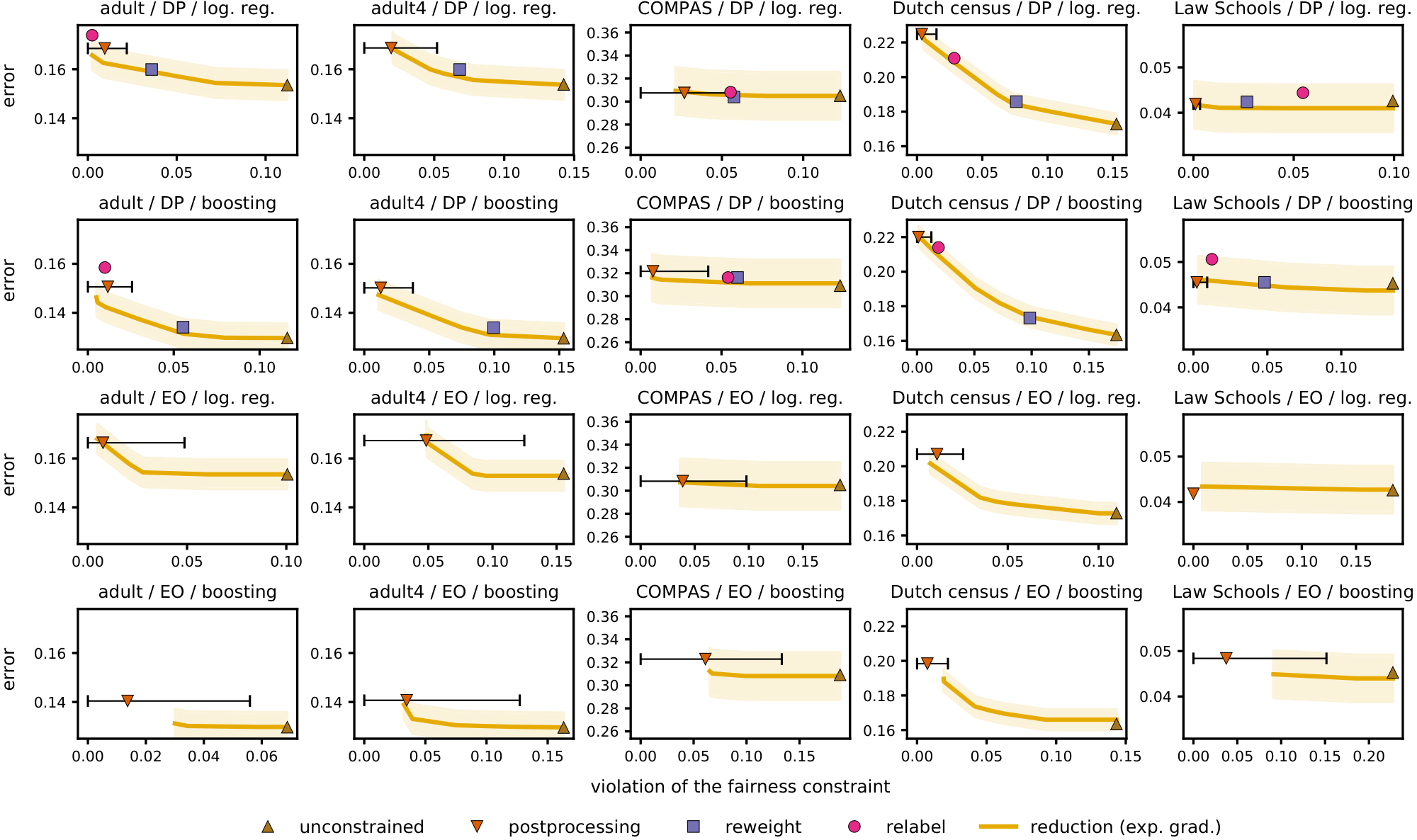
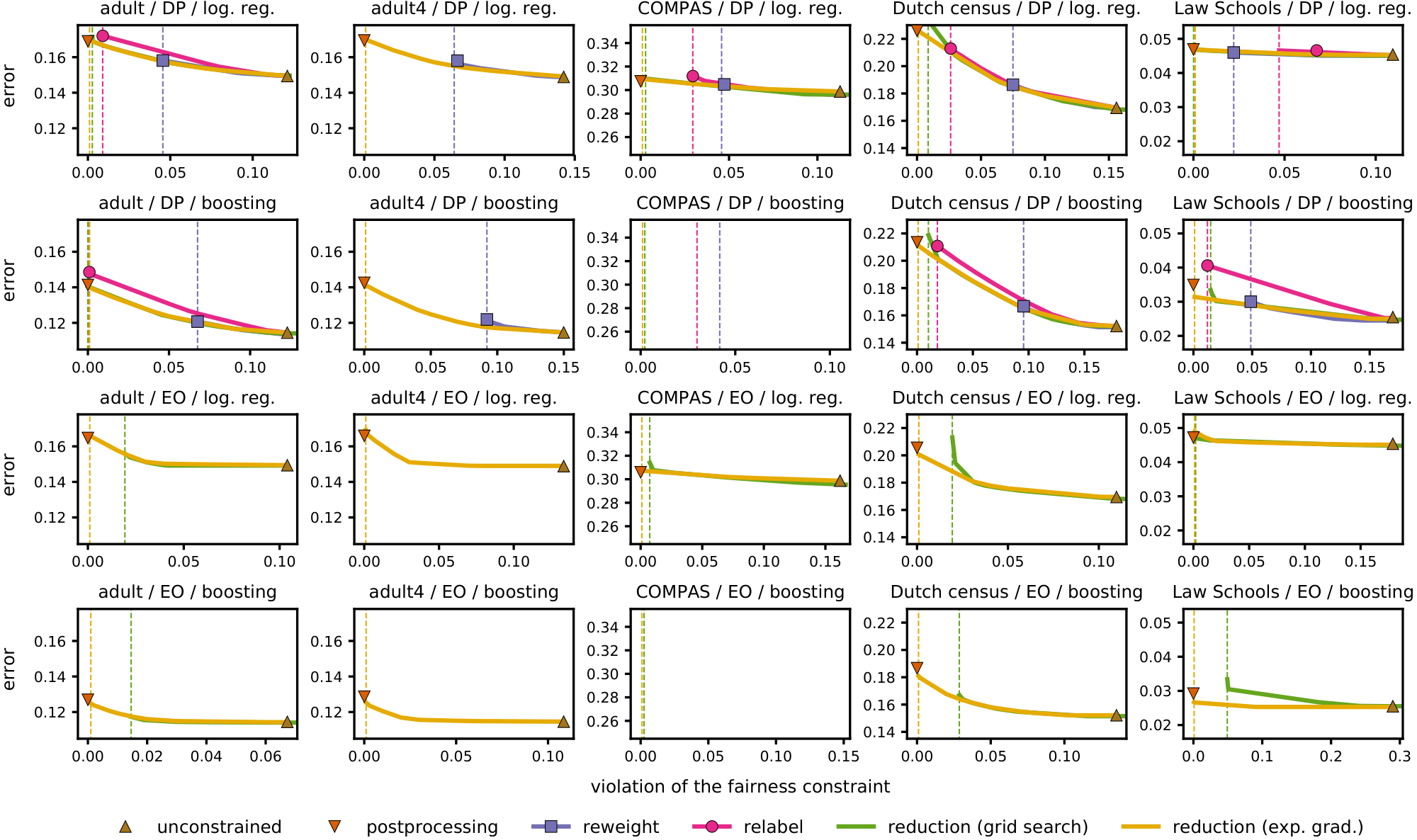
We ran our reduction across a wide range of tradeoffs between the classification error and fairness constraints. We considered $\varepsilon\in{0.001, \dotsc, 0.1}$ and for each value ran Algorithm 1 with $\widehat{c}_k= \varepsilon$ across all $k$. As expected, the returned randomized classifiers tracked the training Pareto frontier (see Figure 2 in Appendix D). In Figure 1, we evaluate these classifiers alongside the baselines on the test data.

For all the data sets, the range of classification errors is much smaller than the range of constraint violations. Almost all the approaches were able to substantially reduce or remove disparity without much impact on classifier accuracy. One exception was the Dutch census data set, where the classification error increased the most in relative terms.

Our reduction generally dominated or matched the baselines. The relabeling approach frequently yielded solutions that were not Pareto optimal. Reweighting yielded solutions on the Pareto frontier, but often with substantial disparity. As expected, post-processing yielded disparities that were statistically indistinguishable from zero, but the resulting classification error was sometimes higher than achieved by our reduction under a statistically indistinguishable disparity. In addition, and unlike the post-processing algorithm, our reduction can achieve any desired accuracy–fairness tradeoff, allows a wider range of fairness definitions, and does not require access to the protected attribute at test time.

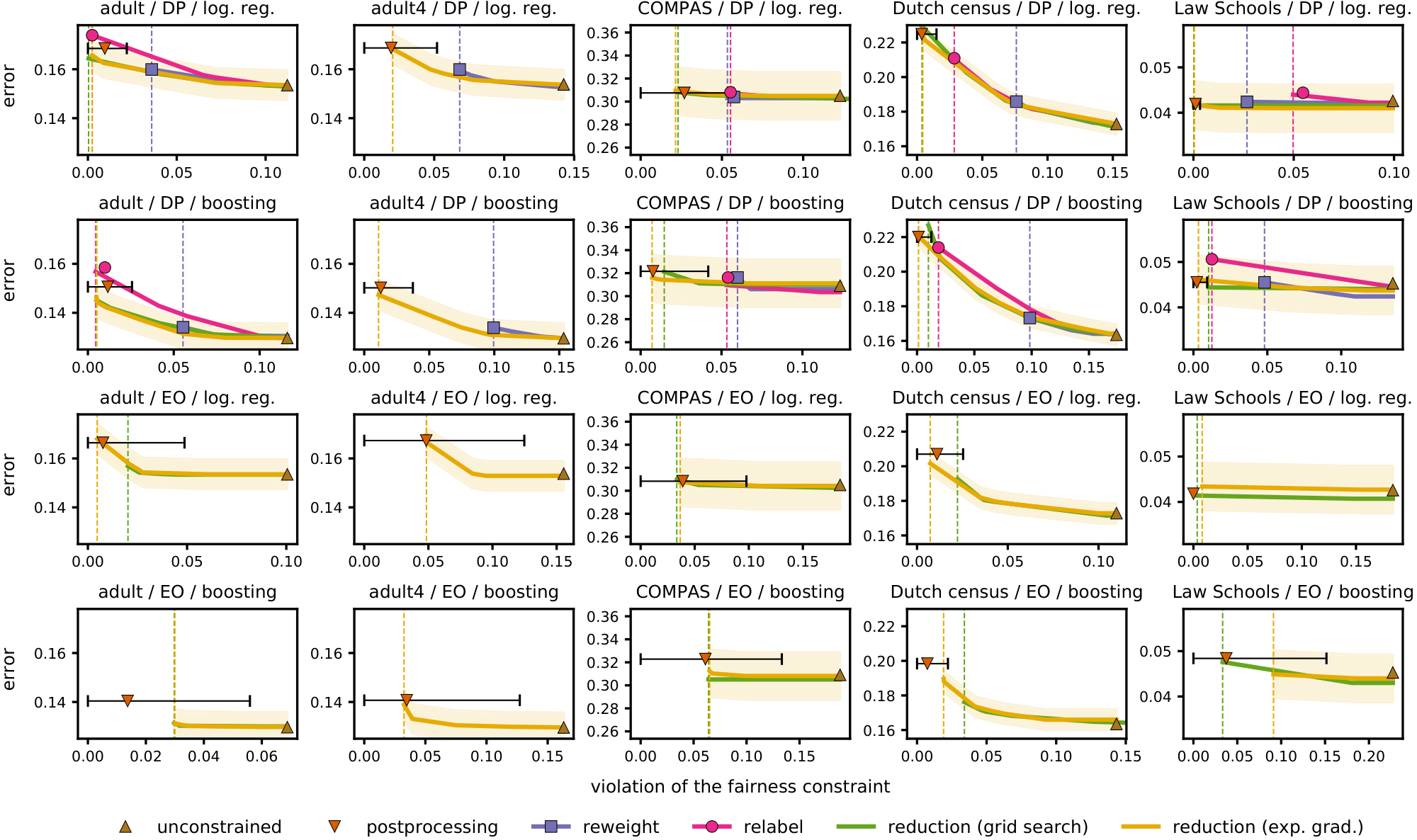
Our grid-search reduction, evaluated in Appendix D, sometimes failed to achieve the lowest disparities on the training data, but its performance on the test data very closely matched that of our exponentiated-gradient reduction. However, if the protected attribute is non-binary, then grid search is not feasible. For instance, for the version of the adult income data set where the protected attribute takes on four values, the grid search would need to span three dimensions for demographic parity and six dimensions for equalized odds, both of which are prohibitively costly.

5. Conclusion

Section Summary: The authors describe two flexible techniques for reducing bias in binary classifiers that apply across many fairness definitions, any underlying model, and practical settings while providing theoretical performance guarantees. These methods balance accuracy against a single fairness goal when sensitive attributes are available during training. The conclusion highlights two remaining challenges: achieving fairness without access to those attributes and managing tradeoffs across multiple fairness goals simultaneously.

We presented two reductions for achieving fairness in a binary classification setting. Our reductions work for any classifier representation, encompass many definitions of fairness, satisfy provable guarantees, and work well in practice.

Our reductions optimize the tradeoff between accuracy and any (single) definition of fairness given training-time access to protected attributes. Achieving fairness when training-time access to protected attributes is unavailable remains an open problem for future research, as does the navigation of tradeoffs between accuracy and multiple fairness definitions.

Acknowledgements

We would like to thank Aaron Roth, Sam Corbett-Davies, and Emma Pierson for helpful discussions.

Appendix

Section Summary: The appendix first extends standard error and fairness definitions to randomized classifiers by expressing both as convex combinations of the corresponding quantities for deterministic classifiers drawn from the distribution. It then proves Theorem 3 by applying known regret bounds for the Exponentiated Gradient algorithm to an online zero-sum game whose players alternately select classifiers and Lagrange multipliers, showing that the time-averaged pair of strategies forms an approximate saddle point of the Lagrangian with explicit sub-optimality controlled by the learning rate and bound parameters. The argument proceeds by rewriting the per-round payoffs, invoking linearity to interchange sums, and chaining the resulting inequalities to bound both sides of the saddle-point condition.

A. Error and Fairness for Randomized Classifiers

Let $D$ denote the distribution over triples $(X, A, Y)$. The accuracy of a classifier $h\in \mathcal{H}$ is measured by 0-1 error, $\textup{err}(h)\coloneqq \mathbb{P}_D[h(X)\ne Y]$, which for a randomized classifier $Q$ becomes

$ \textup{err}(Q)\coloneqq \mathop{\mathbb{P}}{(X, A, Y)\sim D, , h\sim Q}[h(X)\ne Y] =!\sum{h\in \mathcal{H}} Q(h), \textup{err}(h) \enspace . $

The fairness constraints on a classifier $h$ are $\mathbf{M}\boldsymbol{\mu}(h)\le {\mathbf{c}}$. Recall that $\mu_j(h)\coloneqq \mathbb{E}_D[g_j(X, A, Y, h(X))\mathbin{\vert}\mathcal{E}_j]$. For a randomized classifier $Q$ we define its moment $\mu_j$ as

$ \mu_j(Q) \coloneqq \mathop{\mathbb{E}}_{(X, A, Y)\sim D, , h\sim Q} \Bigl[g_j(X, A, Y, h(X))\mathbin{\Bigm\vert}\mathcal{E}j\Bigr] =!\sum{h\in \mathcal{H}} Q(h)\mu_j(h) \enspace, $

where the last equality follows because $\mathcal{E}_j$ is independent of the choice of $h$.

B. Proof of Theorem 3

The proof follows immediately from the analysis of [25] applied to the Exponentiated Gradient (EG) algorithm ([26]), which in our specific case is also equivalent to Hedge ([32]).

Let $\Lambda\coloneqq{\boldsymbol{\lambda}\in \mathbb{R}^{\lvert \mathcal{K}\rvert}+::\lVert\boldsymbol{\lambda}'\rVert_1\le B}$ and $\Lambda'\coloneqq{\boldsymbol{\lambda}'\in \mathbb{R}^{\lvert \mathcal{K}\rvert+1}+::\lVert\boldsymbol{\lambda}'\rVert_1=B}$. We associate any $\boldsymbol{\lambda}\in\Lambda$ with the $\boldsymbol{\lambda}'\in\Lambda'$ that is equal to $\boldsymbol{\lambda}$ on coordinates $1$ through $\lvert \mathcal{K}\rvert$ and puts the remaining mass on the coordinate $\lambda'_{\lvert \mathcal{K}\rvert+1}$.

Consider a run of Algorithm 1. For each $\boldsymbol{\lambda}_t$, let $\boldsymbol{\lambda}'_t\in\Lambda'$ be the associated element of $\Lambda'$. Let $\mathbf{r}_t\coloneqq \mathbf{M}\widehat{\boldsymbol{\mu}}(h_t)-\widehat{\mathbf{c}}$ and let $\mathbf{r}'_t\in \mathbb{R}^{\lvert \mathcal{K}\rvert+1}$ be equal to $\mathbf{r}t$ on coordinates $1$ through $\lvert \mathcal{K}\rvert$ and put zero on the coordinate $r'{t, \lvert \mathcal{K}\rvert+1}$. Thus, for any $\boldsymbol{\lambda}$ and the associated $\boldsymbol{\lambda}'$, we have, for all $t$,

$ \boldsymbol{\lambda}^{!\top}\mathbf{r}_t=(\boldsymbol{\lambda}')^{!\top}\mathbf{r}'_t \enspace,\tag{7} $

and, in particular,

$ \boldsymbol{\lambda}_t ^{!\top}\bigl(\mathbf{M}\widehat{\boldsymbol{\mu}}(h_t)-\widehat{\mathbf{c}}\bigr)

\boldsymbol{\lambda}_t ^{!\top}\mathbf{r}_t

(\boldsymbol{\lambda}'_t)^{!\top}\mathbf{r}'_t \enspace.\tag{8} $

We interpret $\mathbf{r}'_t$ as the reward vector for the $\boldsymbol{\lambda}$-player. The choices of $\boldsymbol{\lambda}'_t$ then correspond to those of the EG algorithm with the learning rate $\eta$. By the assumption of the theorem we have $\lVert \mathbf{r}'t\rVert\infty=\lVert \mathbf{r}t\rVert\infty\le\rho$. The regret bound for EG, specifically, Corollary 2.14 of [33], then states that for any $\boldsymbol{\lambda}'\in\Lambda'$,

$ \sum_{t=1}^T (\boldsymbol{\lambda}')^{!\top}\mathbf{r}'t \le \sum{t=1}^T (\boldsymbol{\lambda}'_t)^{!\top}\mathbf{r}'t + \underbrace{\frac{B\log(\lvert \mathcal{K}\rvert+1)}{\eta}+\eta\rho^2 B T}{\eqqcolon\zeta_T} \enspace. $

Therefore, by equations 7 and 8, we also have for any $\boldsymbol{\lambda}\in\Lambda$,

$ \sum_{t=1}^T \boldsymbol{\lambda}^{!\top}\mathbf{r}t \le \sum{t=1}^T \boldsymbol{\lambda}_t ^{!\top}\mathbf{r}_t + \zeta_T \enspace.\tag{9} $

This regret bound can be used to bound the suboptimality of $L(\widehat{Q}_T, \widehat{\boldsymbol{\lambda}}_T)$ in $\widehat{\boldsymbol{\lambda}}_T$ as follows:

$ \begin{aligned} \notag L(\widehat{Q}T, \boldsymbol{\lambda}) &=\frac{1}{T} \sum{t=1}^T\Bigl(\widehat{\textup{err}}(h_t)+\boldsymbol{\lambda}^{!\top}\bigl(\mathbf{M}\widehat{\boldsymbol{\mu}}(h_t)-\widehat{\mathbf{c}}\bigr)\Bigr) \ \notag &=\frac{1}{T} \sum_{t=1}^T\Bigl(\widehat{\textup{err}}(h_t)+\boldsymbol{\lambda}^{!\top}\mathbf{r}t\Bigr) \ \quad\text{(a)} &\le\frac{1}{T} \sum{t=1}^T\Bigl(\widehat{\textup{err}}(h_t)+\boldsymbol{\lambda}_t ^{!\top}\mathbf{r}t\Bigr) +\frac{\zeta_T}{T} \ \notag &=\frac{1}{T} \sum{t=1}^T L(h_t, \boldsymbol{\lambda}t) +\frac{\zeta_T}{T} \ \quad\text{(b)} &\le\frac{1}{T} \sum{t=1}^T L(\widehat{Q}_T, \boldsymbol{\lambda}_t) +\frac{\zeta_T}{T} \ \quad\text{(c)} &=L\Bigl(\widehat{Q}T, , \frac{1}{T}\sum{t=1}^T \boldsymbol{\lambda}_t\Bigr)+\frac{\zeta_T}{T} =L(\widehat{Q}_T, \widehat{\boldsymbol{\lambda}}_T)+\frac{\zeta_T}{T} \enspace. \end{aligned}\tag{10} $

Equation 10a follows from the regret bound Equation 9. Equation 10b follows because L(h_t, lambda_t)<= L(Q, lambda_t) for all Q by the choice of h_t as the best response of the Q-player. Finally, equation 10c follows by linearity of L(Q, lambda) in lambda. Thus, we have for all lambda in Lambda,

$ L(\widehat{Q}_T, \widehat{\boldsymbol{\lambda}}_T) \ge L(\widehat{Q}_T, \boldsymbol{\lambda})-\frac{\zeta_T}{T} \enspace.\tag{11} $

Also, for any Q,

$ \begin{aligned} \quad\text{(a)} L(Q, \widehat{\boldsymbol{\lambda}}T) &=\frac{1}{T} \sum{t=1}^T L(Q, \boldsymbol{\lambda}t) \ \quad\text{(b)} &\ge\frac{1}{T} \sum{t=1}^T L(h_t, \boldsymbol{\lambda}t) \ \quad\text{(c)} &\ge\frac{1}{T} \sum{t=1}^T L(h_t, \widehat{\boldsymbol{\lambda}}_T)-\frac{\zeta_T}{T} \ \quad\text{(d)} &= L(\widehat{Q}_T, \widehat{\boldsymbol{\lambda}}_T)-\frac{\zeta_T}{T} \enspace, \end{aligned}\tag{12} $

where equation 12a follows by linearity of L(Q, lambda) in lambda, equation 12b follows by the optimality of h_t with respect to lambda_hat_t, equation 12c from the regret bound Equation 9, and equation 12d by linearity of L(Q, lambda) in Q. Thus, for all Q,

$ L(\widehat{Q}_T, \widehat{\boldsymbol{\lambda}}_T) \le L(Q, \widehat{\boldsymbol{\lambda}}_T)+\frac{\zeta_T}{T} \enspace.\tag{13} $

Equations 11 and 13 immediately imply that for any T>= 1,

$ \nu_T\le\frac{\zeta_T}{T}=\frac{B\log(\lvert \mathcal{K}\rvert+1)}{\eta T}+\eta\rho^2 B \enspace, $

proving the first part of the theorem.

The second part of the theorem follows by plugging in eta=(nu)/(2rho^2 B) and verifying that if T>=(4rho^2 B^2log(| K|+1))/(nu^2) then

$ \nu_T \le\frac{B\log(\lvert \mathcal{K}\rvert+1)}{\frac{\nu}{2\rho^2 B}\cdot\frac{4\rho^2 B^2\log(\lvert \mathcal{K}\rvert+1)}{\nu^2}}+\frac{\nu}{2\rho^2 B}\cdot\rho^2 B =\frac{\nu}{2}+\frac{\nu}{2} \enspace. $

C. Proofs of Theorem 5 and Theorem 6

The bulk of this appendix proves the following theorem, which will immediately imply Theorem 5 and Theorem 6.

########## {caption="Theorem 7"}

Let (Q_hat, lambda_hat) be any nu-approximate saddle point of L with

$ {\widehat{c}}k = c_k + \varepsilon_k \quad \text{and} \quad \varepsilon_k\ge\sum{j \in \mathcal{J}} \lvert M_{k, j}\rvert\left(2R_{n_j}(\mathcal{H}) + \frac{2}{\sqrt{n_j}} + \sqrt{\frac{\ln(2/\delta)}{2n_j}} \right) \enspace. $

Let Q^* minimize err(Q) subject to M mu(Q) <= c. Then with probability at least 1-(| J|+1)delta, the distribution Q_hat satisfies

$ \begin{aligned} \textup{err}(\widehat{Q}) & \le \textup{err}(Q^\star) + 2\nu + 4R_n(\mathcal{H}) + \frac{4}{\sqrt{n}} + \sqrt{\frac{2\ln(2/\delta)}{n}} \enspace, \ \text{and for all }k\text{,} \quad \gamma_k(\widehat{Q}) & \le c_k +\frac{1+2\nu}{B} + 2 \varepsilon_k \enspace. \end{aligned} $

Let Lambda:=(lambda in R^| K|_+: ||lambda'||_1<= B) denote the domain of lambda. In the remainder of the section, we assume that we are given a pair (Q_hat, lambda_hat) which is a nu-approximate saddle point of L, i.e.,

$ \begin{aligned}L(\widehat{Q}, \boldsymbol{\widehat{\lambda}}) &\leq L(Q, \boldsymbol{\widehat{\lambda}}) + \nu \quad \text{for all }Q\in\Delta\text{,}\\text{and} \quad L(\widehat{Q}, \boldsymbol{\widehat{\lambda}}) &\geq L(\widehat{Q}, \boldsymbol{\lambda}) - \nu \quad \text{for all }\boldsymbol{\lambda}\in\Lambda\text{.}\end{aligned}\tag{14} $

We first establish that the pair (Q_hat, lambda_hat) satisfies an approximate version of complementary slackness. For the statement and proof of the following lemma, recall that gamma_hat(Q)= Mmu_hat(Q), so the empirical fairness constraints can be written as gamma_hat(Q)<= c_hat and the Lagrangian L can be written as

$ L(Q, \boldsymbol{\lambda})

\widehat{\textup{err}}(Q)+\sum_{k\in \mathcal{K}}\lambda_k(\widehat{\gamma}_k(Q)-\widehat{c}_k) \enspace.\tag{15} $

########## {caption="Lemma 8: Approximate complementary slackness"}

The pair (Q_hat, lambda_hat) satisfies

$ \sum_{k \in \mathcal{K}} \widehat{\lambda}_k({\widehat{\gamma}}_k(\widehat{Q}) - {\widehat{c}}k) \geq B\max{k \in \mathcal{K}} \bigl({\widehat{\gamma}}_k(\widehat{Q}) - {\widehat{c}}k\bigr)+ - \nu \enspace, $

where we abbreviate x_+ = max(x, 0) for any real number x.

Proof: We show that the lemma follows from the optimality conditions Equation 14. We consider a dual variable lambda defined as

$ \begin{aligned} \boldsymbol{\lambda} = \begin{cases} \mathbf{0} &\text{if }\widehat{\boldsymbol{\gamma}}(\widehat{Q})\le \widehat{\mathbf{c}}\text{,} \ B \mathbf{e}_{k^\star} &\text{otherwise, where }k^\star= \operatorname{arg, max}_k[\widehat{\gamma}_k(\widehat{Q})-\widehat{c}_k]\text{,} \end{cases} \end{aligned} $

where e_k denotes the k th vector of the standard basis. Then we have by equations 14 and 15 that

$ \begin{aligned} \widehat{\textup{err}}(\widehat{Q}) + \sum_{k \in \mathcal{K}} \widehat{\lambda}_k({\widehat{\gamma}}_k(\widehat{Q}) - {\widehat{c}}k) & = L(\widehat{Q}, \widehat{\boldsymbol{\lambda}}) \ & \ge L(\widehat{Q}, \boldsymbol{\lambda}) - \nu = \widehat{\textup{err}}(\widehat{Q}) + \sum{k \in \mathcal{K}} \lambda_k({\widehat{\gamma}}_k(\widehat{Q}) - {\widehat{c}}_k) - \nu \enspace, \end{aligned} $

and the lemma follows by our choice of lambda.

Next two lemmas bound the empirical error of Q_hat and also bound the amount by which Q_hat violates the empirical fairness constraints.

########## {caption="Lemma 9: Empirical error bound"}

The distribution Q_hat satisfies err_hat(Q_hat)<= err_hat(Q)+2nu for any Q satisfying the empirical fairness constraints, i.e., any Q such that gamma_hat(Q)<= c_hat.

Proof: Assume that Q satisfies gamma_hat(Q)<= c_hat. Since lambda_hat>= 0, we have

$ L(Q, \widehat{\boldsymbol{\lambda}})= \widehat{\textup{err}}(Q)+ \widehat{\boldsymbol{\lambda}}^{!\top}\bigl(\widehat{\boldsymbol{\gamma}}(Q)-\widehat{\mathbf{c}}\bigr) \le \widehat{\textup{err}}(Q) \enspace. $

The optimality conditions Equation 14 imply that

$ L(\widehat{Q}, \boldsymbol{\widehat{\lambda}}) \leq L(Q, \widehat{\boldsymbol{\lambda}}) + \nu \enspace. $

Putting these together, we obtain

$ L(\widehat{Q}, \widehat{\boldsymbol{\lambda}}) \le \widehat{\textup{err}}(Q)+\nu \enspace. $

We next invoke Lemma 8 to lower bound L(Q_hat, lambda_hat) as

$ \begin{aligned} L(\widehat{Q}, \widehat{\boldsymbol{\lambda}})

\widehat{\textup{err}}(\widehat{Q}) + \sum_{k \in \mathcal{K}} \widehat{\lambda}_k({\widehat{\gamma}}_k(\widehat{Q}) - {\widehat{c}}k) &\geq \widehat{\textup{err}}(\widehat{Q}) + B\max{k \in \mathcal{K}}\bigl({\widehat{\gamma}}_k(\widehat{Q}) - {\widehat{c}}k\bigr)+ - \nu \ &\geq \widehat{\textup{err}}(\widehat{Q}) - \nu \enspace. \end{aligned} $

Combining the upper and lower bounds on L(Q_hat, lambda_hat) completes the proof.

########## {caption="Lemma 10: Empirical fairness violation"}

Assume that the empirical fairness constraints gamma_hat(Q)<= c_hat are feasible. Then the distribution Q_hat approximately satisfies all empirical fairness constraints:

$ \max_{k \in \mathcal{K}} \left({\widehat{\gamma}}_k(\widehat{Q}) - {\widehat{c}}_k\right) \leq \frac{1+2\nu}{B} \enspace. $

Proof: Let Q satisfy gamma_hat(Q)<= c_hat. Applying the same upper and lower bound on L(Q_hat, lambda_hat) as in the proof of Lemma 9, we obtain

$ \widehat{\textup{err}}(\widehat{Q}) + B\max_{k \in \mathcal{K}}\bigl({\widehat{\gamma}}_k(\widehat{Q}) - {\widehat{c}}k\bigr)+ - \nu ;\leq; L(\widehat{Q}, \boldsymbol{\widehat{\lambda}}) ;\leq; \widehat{\textup{err}}(Q) + \nu \enspace. $

We can further upper bound err_hat(Q)-err_hat(Q_hat) by 1 and use x <= x_+ for any real number x to complete the proof.

It remains to lift the bounds on empirical classification error and constraint violation into the corresponding bounds on true classification error and the violation of true constraints. We will use the standard machinery of uniform convergence bounds via the (worst-case) Rademacher complexity.

Let F be a class of functions f: Z->[0, 1] over some space Z. Then the (worst-case) Rademacher complexity of F is defined as

$ R_n(\mathcal{F}) \coloneqq \sup_{z_1, \dotsc, z_n\in \mathcal{Z}} \mathbb{E}\left[\sup_{f\in \mathcal{F}}\left\lvert \frac{1}{n} \sum_{i=1}^n \sigma_i f(z_i) \right\rvert\right] \enspace, $

where the expectation is over the i.i.d. random variables sigma_1, dotsc, sigma_n with P[sigma_i=1]= P[sigma_i=-1]=1/2.

We first prove concentration of generic moments derived from classifiers h in H and then move to bounding the deviations from true classification error and true fairness constraints.

########## {caption="Lemma 11: Concentration of moments"}

Let g: Xx Ax(0, 1)x(0, 1)->[0, 1] be any function and let D be a distribution over (X, A, Y). Then with probability at least 1-delta, for all h in H,

$ \Bigl\lvert \widehat{\mathbb{E}}\bigl[g(X, A, Y, h(X))\bigr]-\mathbb{E}\bigl[g(X, A, Y, h(X))\bigr] \Bigr\rvert \le 2R_n(\mathcal{H}) + \frac{2}{\sqrt{n}} + \sqrt{\frac{\ln(2/\delta)}{2n}} \enspace, $

where the expectation is with respect to D and the empirical expectation is based on n i.i.d. draws from D.

Proof: Let F:=(f_h)_h in H be the class of functions f_h: (x, y, a)-> gbigl(x, y, a, h(x)bigr). By Theorem 3.2 of [34], we then have with probability at least 1-delta, for all h,

$ \Bigl\lvert \widehat{\mathbb{E}}\bigl[g(X, A, Y, h(X))\bigr]-\mathbb{E}\bigl[g(X, A, Y, h(X))\bigr] \Bigr\rvert

\Bigl\lvert \widehat{\mathbb{E}}[f_h]-\mathbb{E}[f_h]\Bigr\rvert \le 2 R_n(\mathcal{F}) + \sqrt{\frac{\ln(2/\delta)}{2n}} \enspace.\tag{16} $

We will next bound R_n(F) in terms of R_n(H). Since h(x) in (0, 1), we can write

$ f_h(x, y, a)=h(x) g(x, a, y, 1) + \Bigl(1-h(x)\Bigr)g(x, a, y, 0) =g(x, a, y, 0)+h(x)\Bigl(g(x, a, y, 1)-g(x, a, y, 0)\Bigr) \enspace. $

Since bigl| g(x, a, y, 0)bigr|<= 1 and bigl| g(x, a, y, 1)-g(x, a, y, 0)bigr|<= 1, we can invoke Theorem 12(5) of [28] for bounding function classes shifted by an offset, in our case g(x, a, y, 0), and Theorem 4.4 of [35] for bounding function classes under contraction, in our case g(x, a, y, 1)-g(x, a, y, 0), yielding

$ R_n(\mathcal{F})\le \frac{1}{\sqrt{n}} + R_n(\mathcal{H}) \enspace. $

Together with the bound Equation 16, this proves the lemma.

########## {caption="Lemma 12: Concentration of loss"}

With probability at least 1-delta, for all Q in Delta,

$ \left| \widehat{\textup{err}}(Q)-\textup{err}(Q) \right| \le 2R_n(\mathcal{H}) + \frac{2}{\sqrt{n}} + \sqrt{\frac{\ln(2/\delta)}{2n}} \enspace. $

Proof: We first use Lemma 11 with g:(x, a, y, y_hat)-> 1(yney_hat) to obtain, with probability 1-delta, for all h,

$ \Bigl\lvert \widehat{\textup{err}}(h)-\textup{err}(h)\Bigr\rvert

\Bigl\lvert \widehat{\mathbb{E}}[f_h]-\mathbb{E}[f_h]\Bigr\rvert \le 2R_n(\mathcal{H}) + \frac{2}{\sqrt{n}} + \sqrt{\frac{\ln(2/\delta)}{2n}} \enspace. $

The lemma now follows for any Q by taking a convex combination of the corresponding bounds on h in H.[^7]

[^7]: The same reasoning applies for general error, err(h) = E[g_err(X, A, Y, h(X))], by using g=g_err in Lemma 11.

Finally, we show a result for the concentration of the empirical constraint violations to their population counterparts. We will actually show the concentration of the individual moments mu_hat_j(Q) to mu_j(Q) uniformly for all Q in Delta. Since M is a fixed matrix not dependent on the data, this also directly implies concentration of the constraints gamma_hat(Q)= Mmu_hat(Q) to gamma(Q)= Mmu(Q). For this result, recall that n_j=|(i in [n]: (X_i, A_i, Y_i) in E_j)| and p^*_j = P[E_j].

########## {caption="Lemma 13: Concentration of conditional moments"}

For any j in J, with probability at least 1-delta, for all Q,

$ \bigl\lvert{\widehat{\mu}}j(Q) - \mu_j(Q)\bigr\rvert \leq 2R{n_j}(\mathcal{H}) + \frac{2}{\sqrt{n_j}} + \sqrt{\frac{\ln(2/\delta)}{2n_j}} \enspace. $

If np^*_j>= 8log(2/delta), then with probability at least 1-delta, for all Q,

$ \bigl\lvert{\widehat{\mu}}j(Q) - \mu_j(Q)\bigr\rvert \leq 2R{np^\star_j/2}(\mathcal{H}) + 2\sqrt{\frac{2}{np^\star_j}} + \sqrt{\frac{\ln(4/\delta)}{np^\star_j}} \enspace. $

Proof: Our proof largely follows the proof of Lemma 2 of [2], with appropriate modifications for our more general constraint definition. Let S_j:=(i in [n]: (X_i, A_i, Y_i) in E_j) be the set of indices such that the corresponding examples fall in the event E_j. Note that we have defined n_j = |S_j|. Let D() denote the joint distribution of (X, A, Y). Then, conditioned on i in S_j, the random variables g_j(X_i, A_i, Y_i, h(X_i)) are i.i.d. draws from the distribution D( mathbinvertE_j), with mean mu_j(h). Applying Lemma 11 with g_j and the distribution D(* mathbinvertE_j) therefore yields, with probability 1-delta, for all h,

$ \bigl\lvert{\widehat{\mu}}j(h) - \mu_j(h)\bigr\rvert \leq 2R{n_j}(\mathcal{H}) + \frac{2}{\sqrt{n_j}} + \sqrt{\frac{\ln(2/\delta)}{2n_j}} \enspace, $

The lemma now follows by taking a convex combination over h.

Proof of Theorem 7: We now use the lemmas derives so far to prove Theorem 7. We first use Lemma 13 to bound the gap between the empirical and population fairness constraints. The lemma implies that with probability at least 1-| J|delta, for all k in K and all Q in Delta,

$ \begin{aligned} \notag \bigl\lvert {\widehat{\gamma}}k(Q) - \gamma_k(Q)\bigr\rvert &= \Bigl\lvert \mathbf{M}k \Bigl(\boldsymbol{{\widehat{\mu}}}(Q) - \boldsymbol{\mu}(Q)\Bigr) \Bigr\rvert \ \notag &\leq \sum{j \in \mathcal{J}} \lvert M{k, j}\rvert\Bigl\lvert \widehat{\mu}j(Q)-\mu_j(Q)\Bigr\rvert \ \notag &\leq \sum{j \in \mathcal{J}} \lvert M_{k, j}\rvert \left(2R_{n_j}(\mathcal{H}) + \frac{2}{\sqrt{n_j}} + \sqrt{\frac{\ln(2/\delta)}{2n_j}} \right) \ &\le \varepsilon_k \enspace. \end{aligned}\tag{17} $

Note that our choice of c_hat along with equation 17 ensure that gamma_hat_k(Q^*) <= c_hat_k for all k in K. Using Lemma 9 allows us to conclude that

$ \widehat{\textup{err}}(\widehat{Q})\le \widehat{\textup{err}}(Q^\star)+2\nu \enspace. $

We now invoke Lemma 12 twice, once for err_hat(Q_hat) and once for err_hat(Q^*), proving the first statement of the theorem.

The above shows that Q^* satisfies the empirical fairness constraints, so we can use Lemma 10, which together with equation 17 yields

$ \gamma_k(\widehat{Q}) \le {\widehat{\gamma}}_k(\widehat{Q}) + \varepsilon_k \le \widehat{c}_k+\frac{1+2\nu}{B}+\varepsilon_k=c_k+\frac{1+2\nu}{B}+2 \varepsilon_k \enspace, $

proving the second statement of the theorem.

We are now ready to prove Theorem 5 and Theorem 6

Proof of Theorem 5: The first part of the theorem follows immediately from Assumption 4 and Theorem 7 (with $\delta/2$ instead of $\delta$). The statement in fact holds with probability at least $1-(\lvert \mathcal{J}\rvert+1)\delta/2$. For the second part, we use the multiplicative Chernoff bound for binomial random variables. Note that $\mathbb{E}[n_j]=np^\star_j$, and we assume that $np^\star_j\ge 8\ln(2/\delta)$, so the multiplicative Chernoff bound implies that $n_j\le np^\star_j/2$ with probability at most $\delta/2$. Taking the union bound across all $j$ and combining with the first part of the theorem then proves the second part.

Proof of Theorem 6: This follows immediately from Theorem 3 and the first part of Theorem 5.

D. Additional Experimental Results

In this appendix we present more complete experimental results. We present experimental results for both the training and test data. We evaluate the exponentiated-gradient as well as the grid-search variants of our reductions. And, finally, we consider extensions of reweighting and relabeling beyond the specific tradeoffs proposed by [7]. Specifically, we introduce a scaling parameter that interpolates between the prescribed tradeoff (specific importance weights or the number of examples to relabel) and the unconstrained classifier (uniform weights or zero examples to relabel). The training data results are shown in Figure 2. The test set results are shown in Figure 3.

References

Section Summary: This section lists dozens of academic papers, books, and data sources that the authors cite throughout their work. Most focus on detecting and reducing bias or unfairness in machine learning systems used for decisions such as hiring, lending, or criminal justice. The remaining references cover related technical tools in optimization, classification algorithms, and publicly available research datasets.

[1] Barocas, S. and Selbst, A. D. Big data's disparate impact. California Law Review, 104:671–732, 2016.

[2] Woodworth, B. E., Gunasekar, S., Ohannessian, M. I., and Srebro, N. Learning non-discriminatory predictors. In Proceedings of the 30th Conference on Learning Theory (COLT), pp. 1920–1953, 2017.

[3] Zafar, M. B., Valera, I., Rodriguez, M. G., and Gummadi, K. P. Fairness constraints: Mechanisms for fair classification. In Proceedings of the 20th International Conference on Artificial Intelligence and Statistics (AISTATS), pp. 962–970, 2017.

[4] Johnson, K. D., Foster, D. P., and Stine, R. A. Impartial predictive modeling: Ensuring fairness in arbitrary models. arXiv:1608.00528, 2016.

[5] Kamishima, T., Akaho, S., and Sakuma, J. Fairness-aware learning through regularization approach. In 2011 IEEE 11th International Conference on Data Mining Workshops, pp. 643–650, 2011.

[6] Donini, M., Oneto, L., Ben-David, S., Shawe-Taylor, J., and Pontil, M. Empirical risk minimization under fairness constraints. 2018. arXiv:1802.08626.

[7] Kamiran, F. and Calders, T. Data preprocessing techniques for classification without discrimination. Knowledge and Information Systems, 33(1):1–33, 2012.

[8] Feldman, M., Friedler, S. A., Moeller, J., Scheidegger, C., and Venkatasubramanian, S. Certifying and removing disparate impact. In Proceedings of the 21st ACM SIGKDD International Conference on Knowledge Discovery and Data Mining, 2015.

[9] Hardt, M., Price, E., and Srebro, N. Equality of opportunity in supervised learning. In Neural Information Processing Systems (NIPS), 2016.

[10] Calmon, F., Wei, D., Vinzamuri, B., Ramamurthy, K. N., and Varshney, K. R. Optimized pre-processing for discrimination prevention. In Advances in Neural Information Processing Systems 30, 2017.

[11] Corbett-Davies, S., Pierson, E., Feller, A., Goel, S., and Huq, A. Algorithmic decision making and the cost of fairness. In Proceedings of the 23rd ACM SIGKDD International Conference on Knowledge Discovery and Data Mining, pp. 797–806, 2017.

[12] Menon, A. K. and Williamson, R. C. The cost of fairness in binary classification. In Proceedings of the Conference on Fiarness, Accountability, and Transparency, 2018.

[13] Dwork, C., Immorlica, N., Kalai, A. T., and Leiserson, M. Decoupled classifiers for group-fair and efficient machine learning. In Conference on Fairness, Accountability and Transparency (FAT$^{ \star!}$), pp. 119–133, 2018.

[14] Agarwal, A., Beygelzimer, A., Dudík, M., and Langford, J. A reductions approach to fair classification. In Fairness, Accountability, and Transparency in Machine Learning (FATML), 2017.

[15] Alabi, D., Immorlica, N., and Kalai, A. T. Unleashing linear optimizers for group-fair learning and optimization. In Proceedings of the 31st Annual Conference on Learning Theory (COLT), 2018.

[16] Kearns, M., Neel, S., Roth, A., and Wu, Z. S. Preventing fairness gerrymandering: Auditing and learning for subgroup fairness. In Proceedings of the 35th International Conference on Machine Learning (ICML), 2018.

[17] Dwork, C., Hardt, M., Pitassi, T., Reingold, O., and Zemel, R. Fairness through awareness. In Proceedings of the 3rd Innovations in Theoretical Computer Science Conference, pp. 214–226, 2012.

[18] Kleinberg, J., Mullainathan, S., and Raghavan, M. Inherent trade-offs in the fair determination of risk scores. In Proceedings of the 8th Innovations in Theoretical Computer Science Conference, 2017.

[19] Chouldechova, A. Fair prediction with disparate impact: A study of bias in recidivism prediction instruments. Big Data, Special Issue on Social and Technical Trade-Offs, 2017.

[20] Berk, R., Heidari, H., Jabbari, S., Kearns, M., and Roth, A. Fairness in criminal justice risk assessments: The state of the art. arXiv:1703.09207, 2017.

[21] Beygelzimer, A., Dani, V., Hayes, T. P., Langford, J., and Zadrozny, B. Error limiting reductions between classification tasks. In Proceedings of the Twenty-Second International Conference on Machine Learning (ICML), pp. 49–56, 2005.

[22] Langford, J. and Beygelzimer, A. Sensitive error correcting output codes. In Proceedings of the 18th Annual Conference on Learning Theory (COLT), pp. 158–172, 2005.

[23] Fan, W., Stolfo, S. J., Zhang, J., and Chan, P. K. Adacost: Misclassification cost-sensitive boosting. In Proceedings of the Sixteenth International Conference on Machine Learning (ICML), pp. 97–105, 1999.

[24] Rockafellar, R. T. Convex analysis. Princeton University Press, 1970.

[25] Freund, Y. and Schapire, R. E. Game theory, on-line prediction and boosting. In Proceedings of the Ninth Annual Conference on Computational Learning Theory (COLT), pp. 325–332, 1996.

[26] Kivinen, J. and Warmuth, M. K. Exponentiated gradient versus gradient descent for linear predictors. Information and Computation, 132(1):1–63, 1997.

[27] Kakade, S. M., Sridharan, K., and Tewari, A. On the complexity of linear prediction: Risk bounds, margin bounds, and regularization. In Advances in neural information processing systems, pp. 793–800, 2009.

[28] Bartlett, P. L. and Mendelson, S. Rademacher and gaussian complexities: Risk bounds and structural results. Journal of Machine Learning Research, 3:463–482, 2002.

[29] Pedregosa, F., Varoquaux, G., Gramfort, A., Michel, V., Thirion, B., Grisel, O., Blondel, M., Prettenhofer, P., Weiss, R., Dubourg, V., Vanderplas, J., Passos, A., Cournapeau, D., Brucher, M., Perrot, M., and Duchesnay, E. Scikit-learn: Machine learning in Python. Journal of Machine Learning Research, 12:2825–2830, 2011.

[30] Lichman, M. UCI machine learning repository, 2013. URL http://archive.ics.uci.edu/ml.

[31] Wightman, L. LSAC National Longitudinal Bar Passage Study, 1998.

[32] Freund, Y. and Schapire, R. E. A decision-theoretic generalization of on-line learning and an application to boosting. Journal of Computer and System Sciences, 55(1):119–139, 1997.

[33] Shalev-Shwartz, S. Online learning and online convex optimization. Foundations and Trends in Machine Learning, 4(2):107–194, 2012.

[34] Boucheron, S., Bousquet, O., and Lugosi, G. Theory of classification: a survey of some recent advances. ESAIM: Probability and Statistics, 9:323–375, 2005.

[35] Ledoux, M. and Talagrand, M. Probability in Banach Spaces: Isoperimetry and Processes. Springer, 1991.