Scaling Distributed Machine Learning with the Parameter Server

Mu Li, Carnegie Mellon University and Baidu; David G. Andersen and Jun Woo Park, Carnegie Mellon University; Alexander J. Smola, Carnegie Mellon University and Google, Inc.; Amr Ahmed, Vanja Josifovski, James Long, Eugene J. Shekita, and Bor-Yiing Su, Google, Inc.

Abstract

We propose a parameter server framework for distributed machine learning problems. Both data and workloads are distributed over worker nodes, while the server nodes maintain globally shared parameters, represented as dense or sparse vectors and matrices. The framework manages asynchronous data communication between nodes, and supports flexible consistency models, elastic scalability, and continuous fault tolerance.

To demonstrate the scalability of the proposed framework, we show experimental results on petabytes of real data with billions of examples and parameters on problems ranging from Sparse Logistic Regression to Latent Dirichlet Allocation and Distributed Sketching.

Executive Summary: The rapid growth of data in applications like web search, advertising, and recommendations has made it impossible for single machines to train complex machine learning models efficiently. These models often involve petabytes of data and billions of parameters, requiring distributed systems to process them quickly. However, challenges such as high network demands, synchronization delays, and frequent hardware failures in cloud environments slow down or disrupt training, leading to lost productivity and higher costs for companies relying on accurate predictions.

This document introduces a parameter server framework designed to address these issues in distributed machine learning. It aims to enable scalable training of models by efficiently sharing and updating parameters across many machines, while supporting a range of algorithms from supervised prediction tasks to unsupervised topic modeling.

The authors developed an open-source system where worker machines process portions of the training data, and dedicated server machines maintain shared model parameters as sparse vectors or matrices. Communication between nodes is asynchronous to avoid blocking computation, with options for flexible consistency levels that balance speed and accuracy. The framework includes built-in fault recovery without restarts and allows adding or removing machines dynamically. To validate it, they ran experiments on real-world datasets from large internet companies, including over 170 billion training examples across 1,000 machines for prediction tasks, 5 billion user records on up to 6,000 machines for topic modeling, and 300 billion streaming events on 15 machines for data summarization. These tests spanned several months on shared production clusters.

Key results show the framework's superior performance. First, for sparse logistic regression on a 636-terabyte ad-click dataset with 65 billion features, it halved training time compared to two custom industry systems, achieving the same model accuracy by reducing worker idle time from over 50% to under 2% through asynchronous updates, and cutting network traffic by up to 50% via data compression and key caching. Second, it filtered out over 93% of unnecessary gradient updates, further speeding convergence. Third, in topic modeling on search logs from 5 billion users and 5 million domains, scaling from 1,000 to 6,000 machines yielded a fourfold speedup in model convergence. Fourth, for streaming data summarization, it processed 1.1 billion inserts per second per cluster with 4.4 gigabits per second bandwidth, recovering from failures in under one second. Finally, the system required only 300 lines of code for capabilities that took over 10,000 lines in specialized alternatives, simplifying development.

These findings mean companies can train more accurate models faster and at lower cost, as the framework tolerates faults and scales elastically without interrupting jobs—critical in unreliable cloud settings where failure rates exceed 20% for large jobs. It outperforms prior systems, like those using rigid synchronization, by adapting to machine learning's tolerance for slight inconsistencies, reducing risks in real-time applications such as ad targeting or fraud detection. Unlike expectations from synchronous frameworks, which struggle beyond hundreds of machines, this approach handles thousands effectively, enabling unprecedented data volumes.

Leaders should deploy this parameter server for large-scale machine learning projects, prioritizing its integration with cluster managers like Yarn for automated resource handling. For immediate gains, start with sparse models in prediction tasks, where traffic reductions yield the biggest time savings; for streaming, pair it with real-time data pipelines. If adapting to new algorithms, conduct pilots to tune consistency delays, as higher delays boost speed but may require 10-20% more iterations. Further work is needed on deeper integration with emerging hardware like GPUs and testing on even larger unsupervised models.

While robust, the system assumes sparse, range-based data patterns common in web tasks, and shared-cluster contention slightly lowered measured speeds. Confidence in scalability is high, backed by production-scale experiments, though caution is advised for dense models where communication overheads could rise.

1 Introduction

Section Summary: Large-scale machine learning problems require distributing computations across multiple machines because no single computer can handle the massive data volumes and complex models with billions to trillions of parameters quickly enough. This setup introduces major hurdles like high network demands for sharing parameters, synchronization delays from sequential algorithms, and frequent failures in cloud environments, as shown by job logs from a data center where failure rates rise sharply with job size due to machine preemptions. The paper introduces an advanced open-source parameter server system that tackles these issues through efficient asynchronous communication, flexible consistency options, elastic scaling without restarts, rapid fault recovery, and user-friendly tools for developers, enabling robust handling of diverse ML tasks at industrial scales.

Distributed optimization and inference is becoming a prerequisite for solving large scale machine learning problems. At scale, no single machine can solve these problems sufficiently rapidly, due to the growth of data and the resulting model complexity, often manifesting itself in an increased number of parameters. Implementing an efficient distributed algorithm, however, is not easy. Both intensive computational workloads and the volume of data communication demand careful system design.

Realistic quantities of training data can range between 1TB and 1PB. This allows one to create powerful and complex models with $10^9$ to $10^{12}$ parameters [9]. These models are often shared globally by all worker nodes, which must frequently accesses the shared parameters as they perform computation to refine it. Sharing imposes three challenges:

• Accessing the parameters requires an enormous amount of network bandwidth.
• Many machine learning algorithms are sequential. The resulting barriers hurt performance when the cost of synchronization and machine latency is high.
• At scale, fault tolerance is critical. Learning tasks are often performed in a cloud environment where machines can be unreliable and jobs can be preempted.

To illustrate the last point, we collected all job logs for a three month period from one cluster at a large internet company. We show statistics of batch machine learning tasks serving a production environment in Table 1. Here, task failure is mostly due to being preempted or losing machines without necessary fault tolerance mechanisms. Unlike in many research settings where jobs run exclusively on a cluster without contention, fault tolerance is a necessity in real world deployments.

: Table 1: Statistics of machine learning jobs for a three month period in a data center.

\begin{tabular}{|r|r|r|}
\hline
$\approx$ \#machine $\times$ time & \# of jobs & failure rate \\
\hline
100 hours & 13,187 & 7.8\% \\
1,000 hours & 1,366 & 13.7\% \\
10,000 hours & 77 & 24.7\% \\
\hline
\end{tabular}

1.1 Contributions

Since its introduction, the parameter server framework [43] has proliferated in academia and industry. This paper describes a third generation open source implementation of a parameter server that focuses on the systems aspects of distributed inference. It confers two advantages to developers: First, by factoring out commonly required components of machine learning systems, it enables application-specific code to remain concise. At the same time, as a shared platform to target for systems-level optimizations, it provides a robust, versatile, and high-performance implementation capable of handling a diverse array of algorithms from sparse logistic regression to topic models and distributed sketching. Our design decisions were guided by the workloads found in real systems. Our parameter server provides five key features:

Efficient communication: The asynchronous communication model does not block computation (unless requested). It is optimized for machine learning tasks to reduce network traffic and overhead.

Flexible consistency models: Relaxed consistency further hides synchronization cost and latency. We allow the algorithm designer to balance algorithmic convergence rate and system efficiency. The best trade-off depends on data, algorithm, and hardware.

Elastic Scalability: New nodes can be added without restarting the running framework.

Fault Tolerance and Durability: Recovery from and repair of non-catastrophic machine failures within 1s, without interrupting computation. Vector clocks ensure well-defined behavior after network partition and failure.

Ease of Use: The globally shared parameters are represented as (potentially sparse) vectors and matrices to facilitate development of machine learning applications. The linear algebra data types come with high-performance multi-threaded libraries.

The novelty of the proposed system lies in the synergy achieved by picking the right systems techniques, adapting them to the machine learning algorithms, and modifying the machine learning algorithms to be more systems-friendly. In particular, we can relax a number of otherwise hard systems constraints since the associated machine learning algorithms are quite tolerant to perturbations. The consequence is the first general purpose ML system capable of scaling to industrial scale sizes.

1.2 Engineering Challenges

When solving distributed data analysis problems, the issue of reading and updating parameters shared between different worker nodes is ubiquitous. The parameter server framework provides an efficient mechanism for aggregating and synchronizing model parameters and statistics between workers. Each parameter server node maintains only a part of the parameters, and each worker node typically requires only a subset of these parameters when operating. Two key challenges arise in constructing a high performance parameter server system:

Communication. While the parameters could be updated as key-value pairs in a conventional datastore, using this abstraction naively is inefficient: values are typically small (floats or integers), and the overhead of sending each update as a key value operation is high.

Our insight to improve this situation comes from the observation that many learning algorithms represent parameters as structured mathematical objects, such as vectors, matrices, or tensors. At each logical time (or an iteration), typically a part of the object is updated. That is, workers usually send a segment of a vector, or an entire row of the matrix. This provides an opportunity to automatically batch both the communication of updates and their processing on the parameter server, and allows the consistency tracking to be implemented efficiently.

Fault tolerance, as noted earlier, is critical at scale, and for efficient operation, it must not require a full restart of a long-running computation. Live replication of parameters between servers supports hot failover. Failover and self-repair in turn support dynamic scaling by treating machine removal or addition as failure or repair respectively.

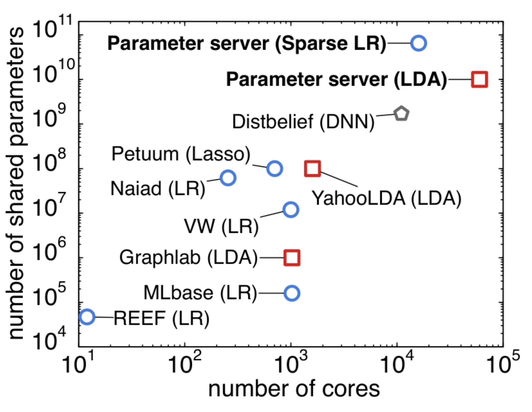
Figure 1 provides an overview of the scale of the largest supervised and unsupervised machine learning experiments performed on a number of systems. When possible, we confirmed the scaling limits with the authors of each of these systems (data current as of 4/2014). As is evident, we are able to cover orders of magnitude more data on orders of magnitude more processors than any other published system. Furthermore, Table 2 provides an overview of the main characteristics of several machine learning systems. Our parameter server offers the greatest degree of flexibility in terms of consistency. It is the only system offering continuous fault tolerance. Its native data types make it particularly friendly for data analysis.

: Table 2: Attributes of distributed data analysis systems.

\begin{tabular}{|l|l|l|l|}
\hline
& Shared Data & Consistency & Fault Tolerance \\
\hline
Graphlab [34] & graph & eventual & checkpoint \\
Petuum [12] & hash table & delay bound & none \\
REEF [10] & array & BSP & checkpoint \\
Naiad [37] & (key,value) & multiple & checkpoint \\
Mlbase [29] & table & BSP & RDD \\
\hline
Parameter & (sparse) & \multirow{2}{*}{various} & \multirow{2}{*}{continuous} \\
Server & vector/matrix & & \\
\hline
\end{tabular}

1.3 Related Work

Related systems have been implemented at Amazon, Baidu, Facebook, Google [13], Microsoft, and Yahoo [1]. Open source codes also exist, such as YahooLDA [1] and Petuum [24]. Furthermore, Graphlab [34] supports parameter synchronization on a best effort model.

The first generation of such parameter servers, as introduced by [43], lacked flexibility and performance — it repurposed memcached distributed (key,value) store as synchronization mechanism. YahooLDA improved this design by implementing a dedicated server with user-definable update primitives (set, get, update) and a more principled load distribution algorithm [1]. This second generation of application specific parameter servers can also be found in Distbelief [13] and the synchronization mechanism of [33]. A first step towards a general platform was undertaken by Petuum [24]. It improves YahooLDA with a bounded delay model while placing further constraints on the worker threading model. We describe a third generation system overcoming these limitations.

Finally, it is useful to compare the parameter server to more general-purpose distributed systems for machine learning. Several of them mandate synchronous, iterative communication. They scale well to tens of nodes, but at large scale, this synchrony creates challenges as the chance of a node operating slowly increases. Mahout [4], based on Hadoop [18] and MLI [44], based on Spark [50], both adopt the iterative MapReduce [14] framework. A key insight of Spark and MLI is preserving state between iterations, which is a core goal of the parameter server.

Distributed GraphLab [34] instead asynchronously schedules communication using a graph abstraction. At present, GraphLab lacks the elastic scalability of the map/reduce-based frameworks, and it relies on coarse-grained snapshots for recovery, both of which impede scalability. Its applicability for certain algorithms is limited by its lack of global variable synchronization as an efficient first-class primitive. In a sense, a core goal of the parameter server framework is to capture the benefits of GraphLab’s asynchrony without its structural limitations.

Piccolo [39] uses a strategy related to the parameter server to share and aggregate state between machines. In it, workers pre-aggregate state locally and transmit the updates to a server keeping the aggregate state. It thus implements largely a subset of the functionality of our system, lacking the machine learning specialized optimizations: message compression, replication, and variable consistency models expressed via dependency graphs.

2 Machine Learning

Section Summary: Machine learning systems help computers learn patterns from examples, like improving web searches or detecting spam, by breaking data into useful features, defining a goal through an objective function that measures success, and iteratively refining a model to meet that goal. These systems handle massive amounts of training data—sometimes trillions of examples from sources like ad logs—requiring efficient processing to update models daily without overwhelming resources. A key approach is risk minimization, which trains models to predict outcomes, such as whether someone will click an ad, by balancing prediction accuracy with model simplicity to avoid errors from overfitting or underfitting.

Machine learning systems are widely used in Web search, spam detection, recommendation systems, computational advertising, and document analysis. These systems automatically learn models from examples, termed training data, and typically consist of three components: feature extraction, the objective function, and learning.

Feature extraction processes the raw training data, such as documents, images and user query logs, to obtain feature vectors, where each feature captures an attribute of the training data. Preprocessing can be executed efficiently by existing frameworks such as MapReduce, and is therefore outside the scope of this paper.

2.1 Goals

The goal of many machine learning algorithms can be expressed via an “objective function.” This function captures the properties of the learned model, such as low error in the case of classifying e-mails into ham and spam, how well the data is explained in the context of estimating topics in documents, or a concise summary of counts in the context of sketching data.

The learning algorithm typically minimizes this objective function to obtain the model. In general, there is no closed-form solution; instead, learning starts from an initial model. It iteratively refines this model by processing the training data, possibly multiple times, to approach the solution. It stops when a (near) optimal solution is found or the model is considered to be converged.

The training data may be extremely large. For instance, a large internet company using one year of an ad impression log [27] to train an ad click predictor would have trillions of training examples. Each training example is typically represented as a possibly very high-dimensional “feature vector” [9]. Therefore, the training data may consist of trillions of trillion-length feature vectors. Iteratively processing such large scale data requires enormous computing and bandwidth resources. Moreover, billions of new ad impressions may arrive daily. Adding this data into the system often improves both prediction accuracy and coverage. But it also requires the learning algorithm to run daily [35], possibly in real time. Efficient execution of these algorithms is the main focus of this paper.

To motivate the design decisions in our system, next we briefly outline the two widely used machine learning technologies that we will use to demonstrate the efficacy of our parameter server. More detailed overviews can be found in [36, 28, 42, 22, 6].

2.2 Risk Minimization

The most intuitive variant of machine learning problems is that of risk minimization. The “risk” is, roughly, a measure of prediction error. For example, if we were to predict tomorrow’s stock price, the risk might be the deviation between the prediction and the actual value of the stock.

The training data consists of $n$ examples. $x_i$ is the $i$th such example, and is often a vector of length $d$. As noted earlier, both $n$ and $d$ may be on the order of billions to trillions of examples and dimensions, respectively. In many cases, each training example $x_i$ is associated with a label $y_i$. In ad click prediction, for example, $y_i$ might be $1$ for “clicked” or $-1$ for “not clicked”.

Risk minimization learns a model that can predict the value $y$ of a future example $x$. The model consists of parameters $w$. In the simplest example, the model parameters might be the “clickiness” of each feature in an ad impression. To predict whether a new impression would be clicked, the system might simply sum its “clickiness” based upon the features present in the impression, namely $x^{\top} w := \sum_{j=1}^d x_j w_j$, and then decide based on the sign.

In any learning algorithm, there is an important relationship between the amount of training data and the model size. A more detailed model typically improves accuracy, but only up to a point: If there is too little training data, a highly-detailed model will overfit and become merely a system that uniquely memorizes every item in the training set. On the other hand, a too-small model will fail to capture interesting and relevant attributes of the data that are important to making a correct decision.

Regularized risk minimization [48, 19] is a method to find a model that balances model complexity and training error. It does so by minimizing the sum of two terms: a loss $\ell(x, y, w)$ representing the prediction error on the training data and a regularizer $\Omega[w]$ penalizing the model complexity. A good model is one with low error and low complexity. Consequently we strive to minimize

$ F(w) = \sum_{i=1}^n \ell(x_i, y_i, w) + \Omega(w).\tag{1} $

The specific loss and regularizer functions used are important to the prediction performance of the machine learning algorithm, but relatively unimportant for the purpose of this paper: the algorithms we present can be used with all of the most popular loss functions and regularizers.

In Section 5.1 we use a high-performance distributed learning algorithm to evaluate the parameter server. For the sake of simplicity we describe a much simpler model called distributed subgradient descent.[^1]

[^1]: The unfamiliar reader could read this as gradient descent; the subgradient aspect is simply a generalization to loss functions and regularizers that need not be continuously differentiable, such as $|w|$ at $w = 0$.

Algorithm 1 Distributed Subgradient Descent
Task Scheduler:
1: issue LoadData() to all workers
2: for iteration $t = 0, \dots, T$ do
3:   issue WORKERITERATE($t$) to all workers.
4: end for
Worker $r = 1, \dots, m$:
1: function LOADDATA()
2:   load a part of training data $\{y_{ik}, x_{ik}\}_{k=1}^{n_r}$
3:   pull the working set $w_r^{(0)}$ from servers
4: end function
5: function WORKERITERATE($t$)
6:   gradient $g_r^{(t)} \leftarrow \sum_{k=1}^{n_r} \partial \ell(x_{ik}, y_{ik}, w_r^{(t)})$
7:   push $g_r^{(t)}$ to servers
8:   pull $w_r^{(t+1)}$ from servers
9: end function
Servers:
1: function SERVERITERATE($t$)
2:   aggregate $g^{(t)} \leftarrow \sum_{r=1}^m g_r^{(t)}$
3:   $w^{(t+1)} \leftarrow w^{(t)} - \eta (g^{(t)} + \partial \Omega(w^{(t)}))$
4: end function

As shown in Figure 2 and Algorithm 1, the training data is partitioned among all of the workers, which jointly learn the parameter vector $w$. The algorithm operates iteratively. In each iteration, every worker independently uses its own training data to determine what changes should be made to $w$ in order to get closer to an optimal value. Because each worker’s updates reflect only its own training data, the system needs a mechanism to allow these updates to mix. It does so by expressing the updates as a subgradient—a direction in which the parameter vector $w$ should be shifted—and aggregates all subgradients before applying them to $w$. These gradients are typically scaled down, with considerable attention paid in algorithm design to the right learning rate $\eta$ that should be applied in order to ensure that the algorithm converges quickly.

The most expensive step in Algorithm 1 is computing the subgradient to update $w$. This task is divided among all of the workers, each of which execute WORKERITERATE. As part of this, workers compute $w^{\top} x_{ik}$, which could be infeasible for very high-dimensional $w$. Fortunately, a worker needs to know a coordinate of $w$ if and only if some of its training data references that entry.

For instance, in ad-click prediction one of the key features are the words in the ad. If only very few advertisements contain the phrase OSDI 2014, then most workers will not generate any updates to the corresponding entry in $w$, and hence do not require this entry. While the total size of $w$ may exceed the capacity of a single machine, the working set of entries needed by a particular worker can be trivially cached locally. To illustrate this, we randomly assigned data to workers and then counted the average working set size per worker on the dataset that is used in Section 5.1. Figure 3 shows that for 100 workers, each worker only needs 7.8% of the total parameters. With 10,000 workers this reduces to 0.15%.

2.3 Generative Models

In a second major class of machine learning algorithms, the label to be applied to training examples is unknown. Such settings call for unsupervised algorithms (for labeled training data one can use supervised or semi-supervised algorithms). They attempt to capture the underlying structure of the data. For example, a common problem in this area is topic modeling: Given a collection of documents, infer the topics contained in each document.

When run on, e.g., the SOSP’13 proceedings, an algorithm might generate topics such as “distributed systems”, “machine learning”, and “performance.” The algorithms infer these topics from the content of the documents themselves, not an external topic list. In practical settings such as content personalization for recommendation systems [2], the scale of these problems is huge: hundreds of millions of users and billions of documents, making it critical to parallelize the algorithms across large clusters.

Because of their scale and data volumes, these algorithms only became commercially applicable following the introduction of the first-generation parameter servers [43]. A key challenge in topic models is that the parameters describing the current estimate of how documents are supposed to be generated must be shared.

A popular topic modeling approach is Latent Dirichlet Allocation (LDA) [7]. While the statistical model is quite different, the resulting algorithm for learning it is very similar to Algorithm 1.[^2] The key difference, however, is that the update step is not a gradient computation, but an estimate of how well the document can be explained by the current model. This computation requires access to auxiliary metadata for each document that is updated each time a document is accessed. Because of the number of documents, metadata is typically read from and written back to disk whenever the document is processed.

[^2]: The specific algorithm we use in the evaluation is a parallelized variant of a stochastic variational sampler [25] with an update strategy similar to that used in YahooLDA [1].

This auxiliary data is the set of topics assigned to each word of a document, and the parameter $w$ being learned consists of the relative frequency of occurrence of a word. As before, each worker needs to store only the parameters for the words occurring in the documents it processes. Hence, distributing documents across workers has the same effect as in the previous section: we can process much bigger models than a single worker may hold.

3 Architecture

Section Summary: The parameter server architecture organizes computing nodes into a central server group that stores and manages shared parameters for machine learning models, divided among multiple servers for reliability and scalability, while worker groups handle the actual computations like calculating gradients from local data. Workers communicate only with servers to update or retrieve parameters, guided by a scheduler that assigns and monitors tasks, allowing multiple groups to run independent or shared applications without interference. This setup uses simple key-value pairs optimized for math operations, efficient range-based data transfers, and flexible features like custom server functions to make building distributed machine learning easier.

An instance of the parameter server can run more than one algorithm simultaneously. Parameter server nodes are grouped into a server group and several worker groups as shown in Figure 4. A server node in the server group maintains a partition of the globally shared parameters. Server nodes communicate with each other to replicate and/or to migrate parameters for reliability and scaling. A server manager node maintains a consistent view of the metadata of the servers, such as node liveness and the assignment of parameter partitions.

Each worker group runs an application. A worker typically stores locally a portion of the training data to compute local statistics such as gradients. Workers communicate only with the server nodes (not among themselves), updating and retrieving the shared parameters. There is a scheduler node for each worker group. It assigns tasks to workers and monitors their progress. If workers are added or removed, it reschedules unfinished tasks.

The parameter server supports independent parameter namespaces. This allows a worker group to isolate its set of shared parameters from others. Several worker groups may also share the same namespace: we may use more than one worker group to solve the same deep learning application [13] to increase parallelization. Another example is that of a model being actively queried by some nodes, such as online services consuming this model. Simultaneously the model is updated by a different group of worker nodes as new training data arrives.

The parameter server is designed to simplify developing distributed machine learning applications such as those discussed in Section 2. The shared parameters are presented as (key,value) vectors to facilitate linear algebra operations (Sec. 3.1). They are distributed across a group of server nodes (Sec. 4.3). Any node can both push out its local parameters and pull parameters from remote nodes (Sec. 3.2). By default, workloads, or tasks, are executed by worker nodes; however, they can also be assigned to server nodes via user defined functions (Sec. 3.3). Tasks are asynchronous and run in parallel (Sec. 3.4). The parameter server provides the algorithm designer with flexibility in choosing a consistency model via the task dependency graph (Sec. 3.5) and predicates to communicate a subset of parameters (Sec. 3.6).

3.1 (Key,Value) Vectors

The model shared among nodes can be represented as a set of (key, value) pairs. For example, in a loss minimization problem, the pair is a feature ID and its weight. For LDA, the pair is a combination of the word ID and topic ID, and a count. Each entry of the model can be read and written locally or remotely by its key. This (key,value) abstraction is widely adopted by existing approaches [37, 29, 12].

Our parameter server improves upon this basic approach by acknowledging the underlying meaning of these key value items: machine learning algorithms typically treat the model as a linear algebra object. For instance, $w$ is used as a vector for both the objective function (1) and the optimization in Algorithm 1 by risk minimization. By treating these objects as sparse linear algebra objects, the parameter server can provide the same functionality as the (key,value) abstraction, but admits important optimized operations such as vector addition $w + u$, multiplication $Xw$, finding the 2-norm $|w|_2$, and other more sophisticated operations [16].

To support these optimizations, we assume that the keys are ordered. This lets us treat the parameters as (key,value) pairs while endowing them with vector and matrix semantics, where non-existing keys are associated with zeros. This helps with linear algebra in machine learning. It reduces the programming effort to implement optimization algorithms. Beyond convenience, this interface design leads to efficient code by leveraging CPU-efficient multithreaded self-tuning linear algebra libraries such as BLAS [16], LAPACK [3], and ATLAS [49].

3.2 Range Push and Pull

Data is sent between nodes using push and pull operations. In Algorithm 1 each worker pushes its entire local gradient into the servers, and then pulls the updated weight back. The more advanced algorithm described in Algorithm 3 uses the same pattern, except that only a range of keys is communicated each time.

The parameter server optimizes these updates for programmer convenience as well as computational and network bandwidth efficiency by supporting range-based push and pull. If $\mathcal{R}$ is a key range, then w.push(R, dest) sends all existing entries of $w$ in key range $\mathcal{R}$ to the destination, which can be either a particular node, or a node group such as the server group. Similarly, w.pull(R, dest) reads all existing entries of $w$ in key range $\mathcal{R}$ from the destination. If we set $\mathcal{R}$ to be the whole key range, then the whole vector $w$ will be communicated. If we set $\mathcal{R}$ to include a single key, then only an individual entry will be sent.

This interface can be extended to communicate any local data structures that share the same keys as $w$. For example, in Algorithm 1, a worker pushes its temporary local gradient $g$ to the parameter server for aggregation. One option is to make $g$ globally shared. However, note that $g$ shares the keys of the worker’s working set $w$. Hence the programmer can use w.push(R, g, dest) for the local gradients to save memory and also enjoy the optimization discussed in the following sections.

3.3 User-Defined Functions on the Server

Beyond aggregating data from workers, server nodes can execute user-defined functions. It is beneficial because the server nodes often have more complete or up-to-date information about the shared parameters. In Algorithm 1, server nodes evaluate subgradients of the regularizer $\Omega$ in order to update $w$. At the same time a more complicated proximal operator is solved by the servers to update the model in Algorithm 3. In the context of sketching (Sec. 5.3), almost all operations occur on the server side.

3.4 Asynchronous Tasks and Dependency

A task is issued by a remote procedure call. It can be a push or a pull that a worker issues to servers. It can also be a user-defined function that the scheduler issues to any node. Tasks may include any number of subtasks. For example, the task WorkerIterate in Algorithm 1 contains one push and one pull.

Tasks are executed asynchronously: the caller can perform further computation immediately after issuing a task. The caller marks a task as finished only once it receives the callee’s reply. A reply could be the function return of a user-defined function, the (key,value) pairs requested by the pull, or an empty acknowledgement. The callee marks a task as finished only if the call of the task is returned and all subtasks issued by this call are finished.

By default, callees execute tasks in parallel, for best performance. A caller that wishes to serialize task execution can place an execute-after-finished dependency between tasks. Figure 5 depicts three example iterations of WorkerIterate. Iterations 10 and 11 are independent, but 12 depends on 11. The callee therefore begins iteration 11 immediately after the local gradients are computed in iteration 10. Iteration 12, however, is postponed until the pull of 11 finishes.

Task dependencies help implement algorithm logic. For example, the aggregation logic in ServerIterate of Algorithm 1 updates the weight $w$ only after all worker gradients have been aggregated. This can be implemented by having the updating task depend on the push tasks of all workers. The second important use of dependencies is to support the flexible consistency models described next.

3.5 Flexible Consistency

Independent tasks improve system efficiency via parallelizing the use of CPU, disk and network bandwidth. However, this may lead to data inconsistency between nodes. In the diagram above, the worker $r$ starts iteration 11 before $w_r^{(11)}$ has been pulled back, so it uses the old $w_r^{(10)}$ in this iteration and thus obtains the same gradient as in iteration 10, namely $g_r^{(11)} = g_r^{(10)}$. This inconsistency potentially slows down the convergence progress of Algorithm 1. However, some algorithms may be less sensitive to this type of inconsistency. For example, only a segment of $w$ is updated each time in Algorithm 3. Hence, starting iteration 11 without waiting for 10 causes only a part of $w$ to be inconsistent.

The best trade-off between system efficiency and algorithm convergence rate usually depends on a variety of factors, including the algorithm’s sensitivity to data inconsistency, feature correlation in training data, and capacity difference of hardware components. Instead of forcing the user to adopt one particular dependency that may be ill-suited to the problem, the parameter server gives the algorithm designer flexibility in defining consistency models. This is a substantial difference to other machine learning systems.

We show three different models that can be implemented by task dependency. Their associated directed acyclic graphs are given in Figure 6.

Sequential In sequential consistency, all tasks are executed one by one. The next task can be started only if the previous one has finished. It produces results identical to the single-thread implementation, and also named Bulk Synchronous Processing.

Eventual Eventual consistency is the opposite: all tasks may be started simultaneously. For instance, [43] describes such a system. However, this is only recommendable if the underlying algorithms are robust with regard to delays.

Bounded Delay When a maximal delay time $\tau$ is set, a new task will be blocked until all previous tasks $\tau$ times ago have been finished. Algorithm 3 uses such a model. This model provides more flexible controls than the previous two: $\tau = 0$ is the sequential consistency model, and an infinite delay $\tau = \infty$ becomes the eventual consistency model.

Note that the dependency graphs may be dynamic. For instance the scheduler may increase or decrease the maximal delay according to the runtime progress to balance system efficiency and convergence of the underlying optimization algorithm. In this case the caller traverses the DAG. If the graph is static, the caller can send all tasks with the DAG to the callee to reduce synchronization cost.

3.6 User-defined Filters

Complementary to a scheduler-based flow control, the parameter server supports user-defined filters to selectively synchronize individual (key,value) pairs, allowing fine-grained control of data consistency within a task. The insight is that the optimization algorithm itself usually possesses information on which parameters are most useful for synchronization. One example is the significantly modified filter, which only pushes entries that have changed by more than a threshold since their last synchronization. In Section 5.1, we discuss another filter named KKT which takes advantage of the optimality condition of the optimization problem: a worker only pushes gradients that are likely to affect the weights on the servers.

Algorithm 2 Set vector clock to $t$ for range $\mathcal{R}$ and node $i$
1: for $S \in \{S_i : S_i \cap \mathcal{R} \neq \emptyset, i = 1, \dots, n\}$ do
2:   if $S \subseteq \mathcal{R}$ then $vc_i(S) \leftarrow t$ else
3:     $a \leftarrow \max(S^b, R^b)$ and $b \leftarrow \min(S^e, R^e)$
4:     split range $S$ into $[S^b, a), [a, b), [b, S^e)$
5:     $vc_i([a, b)) \leftarrow t$
6:   end if
7: end for

4 Implementation

Section Summary: The parameter server system stores data as key-value pairs across multiple servers using consistent hashing to distribute workloads evenly, while replicating entries to nearby servers for fault tolerance through a chain replication method. To handle complex dependencies efficiently, it employs compressed vector clocks that track timestamps for groups of keys in ranges rather than individually, saving significant memory and bandwidth since many parameters update together. Messages between nodes carry these compressed data packets and can be optimized by caching repeated keys, sending only nonzero values, and using compression tools to speed up communication in machine learning tasks.

The servers store the parameters (key-value pairs) using consistent hashing [45] (Sec. 4.3). For fault tolerance, entries are replicated using chain replication [47] (Sec. 4.4). Different from prior (key,value) systems, the parameter server is optimized for range based communication with compression on both data (Sec. 4.2) and range based vector clocks (Sec. 4.1).

4.1 Vector Clock

Given the potentially complex task dependency graph and the need for fast recovery, each (key,value) pair is associated with a vector clock [30, 15], which records the time of each individual node on this (key,value) pair. Vector clocks are convenient, e.g., for tracking aggregation status or rejecting doubly sent data. However, a naive implementation of the vector clock requires $O(nm)$ space to handle $n$ nodes and $m$ parameters. With thousands of nodes and billions of parameters, this is infeasible in terms of memory and bandwidth.

Fortunately, many parameters share the same timestamp as a result of the range-based communication pattern of the parameter server: If a node pushes the parameters in a range, then the timestamps of the parameters associated with the node are likely the same. Therefore, they can be compressed into a single range vector clock. More specifically, assume that $vc_i(k)$ is the time of key $k$ for node $i$. Given a key range $\mathcal{R}$, the ranged vector clock $vc_i(\mathcal{R}) = t$ means for any key $k \in \mathcal{R}, vc_i(k) = t$.

Initially, there is only one range vector clock for each node $i$. It covers the entire parameter key space as its range with 0 as its initial timestamp. Each range set may split the range and create at most 3 new vector clocks (see Algorithm 2). Let $k$ be the total number of unique ranges communicated by the algorithm, then there are at most $O(mk)$ vector clocks, where $m$ is the number of nodes. $k$ is typically much smaller than the total number of parameters. This significantly reduces the space required for range vector clocks.[^3]

[^3]: Ranges can also be merged to reduce the number of fragments. However, in practice both $m$ and $k$ are small enough to be easily handled. We leave merging for future work.

4.2 Messages

Nodes may send messages to individual nodes or node groups. A message consists of a list of (key,value) pairs in the key range $\mathcal{R}$ and the associated range vector clock:

$ [vc(\mathcal{R}), (k_1, v_1), \ldots, (k_p, v_p)] \quad k_j \in \mathcal{R} \text{ and } j \in {1, \ldots p} $

This is the basic communication format of the parameter server not only for shared parameters but also for tasks. For the latter, a (key,value) pair might assume the form (task ID, arguments or return results).

Messages may carry a subset of all available keys within range $\mathcal{R}$. The missing keys are assigned the same timestamp without changing their values. A message can be split by the key range. This happens when a worker sends a message to the whole server group, or when the key assignment of the receiver node has changed. By doing so, we partition the (key,value) lists and split the range vector clock similar to Algorithm 2.

Because machine learning problems typically require high bandwidth, message compression is desirable. Training data often remains unchanged between iterations. A worker might send the same key lists again. Hence it is desirable for the receiving node to cache the key lists. Later, the sender only needs to send a hash of the list rather than the list itself. Values, in turn, may contain many zero entries. For example, a large portion of parameters remain unchanged in sparse logistic regression, as evaluated in Section 5.1. Likewise, a user-defined filter may also zero out a large fraction of the values (see Figure 12). Hence we need only send nonzero (key,value) pairs. We use the fast Snappy compression library [21] to compress messages, effectively removing the zeros. Note that key caching and value-compression can be used jointly.

4.3 Consistent Hashing

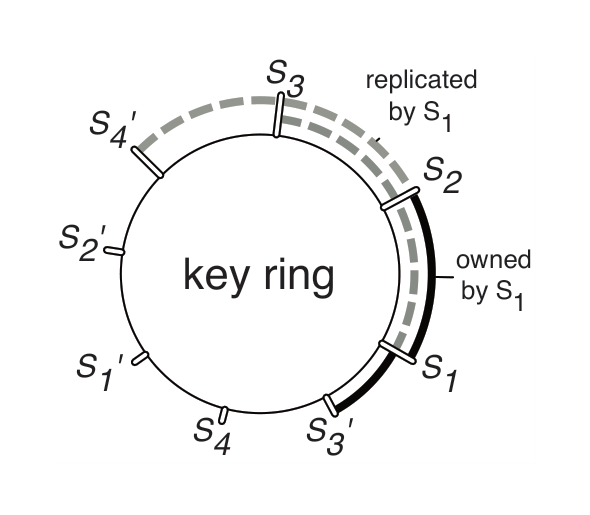
The parameter server partitions keys much as a conventional distributed hash table does [8, 41]: keys and server node IDs are both inserted into the hash ring (Figure 7). Each server node manages the key range starting with its insertion point to the next point by other nodes in the counter-clockwise direction. This node is called the master of this key range. A physical server is often represented in the ring via multiple “virtual” servers to improve load balancing and recovery.

We simplify the management by using a direct-mapped DHT design. The server manager handles the ring management. All other nodes cache the key partition locally. This way they can determine directly which server is responsible for a key range, and are notified of any changes.

4.4 Replication and Consistency

Each server node stores a replica of the $k$ counter-clockwise neighbor key ranges relative to the one it owns. We refer to nodes holding copies as slaves of the appropriate key range. The above diagram shows an example with $k = 2$, where server 1 replicates the key ranges owned by server 2 and server 3.

Worker nodes communicate with the master of a key range for both push and pull. Any modification on the master is copied with its timestamp to the slaves. Modifications to data are pushed synchronously to the slaves. Figure 8 shows a case where worker 1 pushes $x$ into server 1, which invokes a user defined function $f$ to modify the shared data. The push task is completed only once the data modification $f(x)$ is copied to the slave.

Naive replication potentially increases the network traffic by $k$ times. This is undesirable for many machine learning applications that depend on high network bandwidth. The parameter server framework permits an important optimization for many algorithms: replication after aggregation. Server nodes often aggregate data from the worker nodes, such as summing local gradients. Servers may therefore postpone replication until aggregation is complete. In the righthand side of the diagram, two workers push $x$ and $y$ to the server, respectively. The server first aggregates the push by $x + y$, then applies the modification $f(x+y)$, and finally performs the replication. With $n$ workers, replication uses only $k/n$ bandwidth. Often $k$ is a small constant, while $n$ is hundreds to thousands. While aggregation increases the delay of the task reply, it can be hidden by relaxed consistency conditions.

4.5 Server Management

To achieve fault tolerance and dynamic scaling we must support addition and removal of nodes. For convenience we refer to virtual servers below. The following steps happen when a server joins.

1. The server manager assigns the new node a key range to serve as master. This may cause another key range to split or be removed from a terminated node.
2. The node fetches the range of data to maintains as master and $k$ additional ranges to keep as slave.
3. The server manager broadcasts the node changes. The recipients of the message may shrink their own data based on key ranges they no longer hold and to resubmit unfinished tasks to the new node.

Fetching the data in the range $\mathcal{R}$ from some node $S$ proceeds in two stages, similar to the Ouroboros protocol [38]. First $S$ pre-copies all (key,value) pairs in the range together with the associated vector clocks. This may cause a range vector clock to split similar to Algorithm 2. If the new node fails at this stage, $S$ remains unchanged. At the second stage $S$ no longer accepts messages affecting the key range $\mathcal{R}$ by dropping the messages without executing and replying. At the same time, $S$ sends the new node all changes that occurred in $\mathcal{R}$ during the pre-copy stage.

On receiving the node change message a node $N$ first checks if it also maintains the key range $\mathcal{R}$. If true and if this key range is no longer to be maintained by $N$, it deletes all associated (key,value) pairs and vector clocks in $\mathcal{R}$. Next, $N$ scans all outgoing messages that have not received replies yet. If a key range intersects with $\mathcal{R}$, then the message will be split and resent.

Due to delays, failures, and lost acknowledgements $N$ may send messages twice. Due to the use of vector clocks both the original recipient and the new node are able to reject this message and it does not affect correctness.

The departure of a server node (voluntary or due to failure) is similar to a join. The server manager tasks a new node with taking the key range of the leaving node. The server manager detects node failure by a heartbeat signal. Integration with a cluster resource manager such as Yarn [17] or Mesos [23] is left for future work.

4.6 Worker Management

Adding a new worker node $W$ is similar but simpler than adding a new server node:

1. The task scheduler assigns $W$ a range of data.
2. This node loads the range of training data from a network file system or existing workers. Training data is often read-only, so there is no two-phase fetch. Next, $W$ pulls the shared parameters from servers.
3. The task scheduler broadcasts the change, possibly causing other workers to free some training data.

When a worker departs, the task scheduler may start a replacement. We give the algorithm designer the option to control recovery for two reasons: If the training data is huge, recovering a worker node be may more expensive than recovering a server node. Second, losing a small amount of training data during optimization typically affects the model only a little. Hence the algorithm designer may prefer to continue without replacing a failed worker. It may even be desirable to terminate the slowest workers.

5 Evaluation

Section Summary: The evaluation section tests a parameter server system on tasks like sparse logistic regression, which predicts ad clicks using a massive 170-billion-example dataset, and other methods like Latent Dirichlet Allocation, running experiments across clusters at big internet companies and a university. For sparse logistic regression, the system uses 1000 machines to handle the complex algorithm, outperforming two custom-built rivals by cutting network traffic and allowing workers to stay busy without waiting, which halves overall processing time. Results show quicker progress toward accurate models, with workers idle less than 2% of the time compared to over 30% in the competitors.

We evaluate our parameter server based on the use cases of Section 2 — Sparse Logistic Regression and Latent Dirichlet Allocation. We also show results of sketching to illustrate the generality of our framework. The experiments were run on clusters in two (different) large internet companies and a university research cluster to demonstrate the versatility of our approach.

5.1 Sparse Logistic Regression

Problem and Data: Sparse logistic regression is one of the most popular algorithms for large scale risk minimization [9]. It combines the logistic loss[^4] with the $\ell_1$ regularizer[^5] of Section 2.2. The latter biases a compact solution with a large portion of 0 value entries. The non-smoothness of this regularizer, however, makes learning more difficult.

[^4]: $\ell(x_i, y_i, w) = \log(1 + \exp(-y_i x_i, w))$

[^5]: $\Omega(w) = \sum_{i=1}^n |w_i|$

We collected an ad click prediction dataset with 170 billion examples and 65 billion unique features. This dataset is 636 TB uncompressed (141 TB compressed). We ran the parameter server on 1000 machines, each with 16 physical cores, 192GB DRAM, and connected by 10 Gb Ethernet. 800 machines acted as workers, and 200 were parameter servers. The cluster was in concurrent use by other (unrelated) tasks during operation.

Algorithm: We used a state-of-the-art distributed regression algorithm (Algorithm 3, [31, 32]). It differs from the simpler variant described earlier in four ways: First, only a block of parameters is updated in an iteration. Second, the workers compute both gradients and the diagonal part of the second derivative on this block. Third, the parameter servers themselves must perform complex computation: the servers update the model by solving a proximal operator based on the aggregated local gradients. Fourth, we use a bounded-delay model over iterations and use a “KKT” filter to suppress transmission of parts of the generated gradient update that are small enough that their effect is likely to be negligible.[^6]

[^6]: A user-defined Karush-Kuhn-Tucker (KKT) filter [26]. Feature $k$ is filtered if $w_k = 0$ and $|\hat{g}_k| \leq \Delta$. Here $\hat{g}_k$ is an estimate of the global gradient based on the worker’s local information and $\Delta > 0$ is a user-defined parameter.

Algorithm 3 Delayed Block Proximal Gradient [31]
Scheduler:
1: Partition features into $b$ ranges $R_1, \dots, R_b$
2: for $t = 0$ to $T$ do
3:   Pick random range $R_{it}$ and issue task to workers
4: end for
Worker $r$ at iteration $t$
1: Wait until all iterations before $t - \tau$ are finished
2: Compute first-order gradient $g_r^{(t)}$ and diagonal second-order gradient $u_r^{(t)}$ on range $R_{it}$
3: Push $g_r^{(t)}$ and $u_r^{(t)}$ to servers with the KKT filter
4: Pull $w_r^{(t+1)}$ from servers
Servers at iteration $t$
1: Aggregate gradients to obtain $g^{(t)}$ and $u^{(t)}$
2: Solve the proximal operator

   $
   w^{(t+1)} \leftarrow \text{argmin}_u \Omega(u) + \frac{1}{2\eta} \|u - (w^{(t)} - \eta g^{(t)})\|_H^2,
   $

   where $H = \text{diag}(h^{(t)})$ and $\|x\|_H^2 = x^{\top} H x$

To the best of our knowledge, no open source system can scale sparse logistic regression to the scale described in this paper.[^7] We compare the parameter server with two special-purpose systems, named System A and B, developed by a large internet company.

[^7]: Graphlab provides only a multi-threaded, single machine implementation, while Petuum, Mlbase and REEF do not support sparse logistic regression. We confirmed this with the authors as per 4/2014.

Notably, both Systems A and B consist of more than 10K lines of code. The parameter server only requires 300 lines of code for the same functionality as System B.[^8] The parameter server successfully moves most of the system complexity from the algorithmic implementation into a reusable generalized component.

[^8]: System B was developed by an author of this paper.

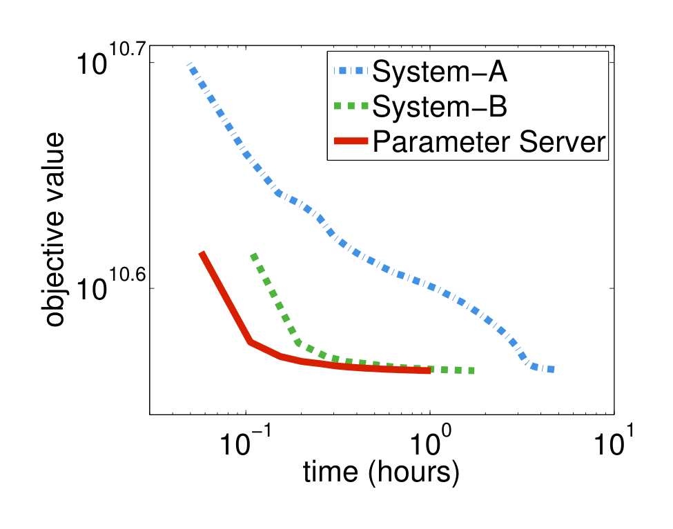
Results: We first compare these three systems by running them to reach the same objective value. A better system achieves a lower objective in less time. Figure 9 shows the results: System B outperforms system A because it uses a better algorithm. The parameter server, in turn, outperforms System B while using the same algorithm. It does so because of the efficacy of reducing the network traffic and the relaxed consistency model.

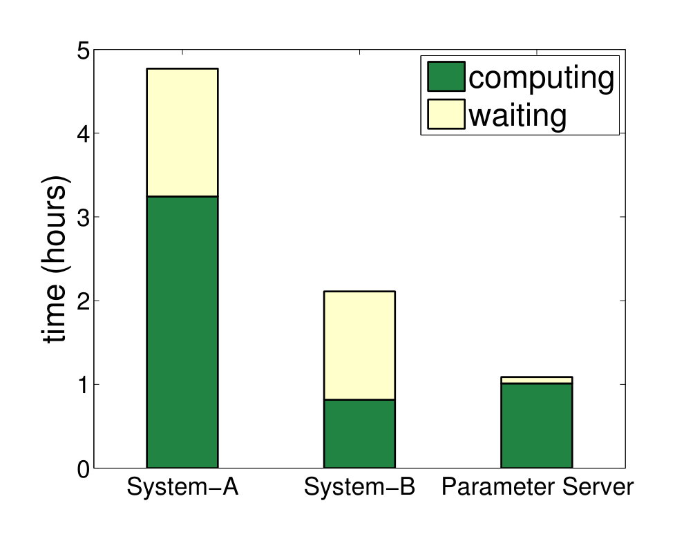
Figure 10 shows that the relaxed consistency model substantially increases worker node utilization. Workers can begin processing the next block without waiting for the previous one to finish, hiding the delay otherwise imposed by barrier synchronization. Workers in System A are 32% idle, and in system B, they are 53% idle, while waiting for the barrier in each block. The parameter server reduces this cost to under 2%. This is not entirely free: the parameter server uses slightly more CPU than System B for two reasons: First, and less fundamentally, System B optimizes its gradient calculations by careful data preprocessing. Second, asynchronous updates with the parameter server require more iterations to achieve the same objective value. Due to the significantly reduced communication cost, the parameter server halves the total time.

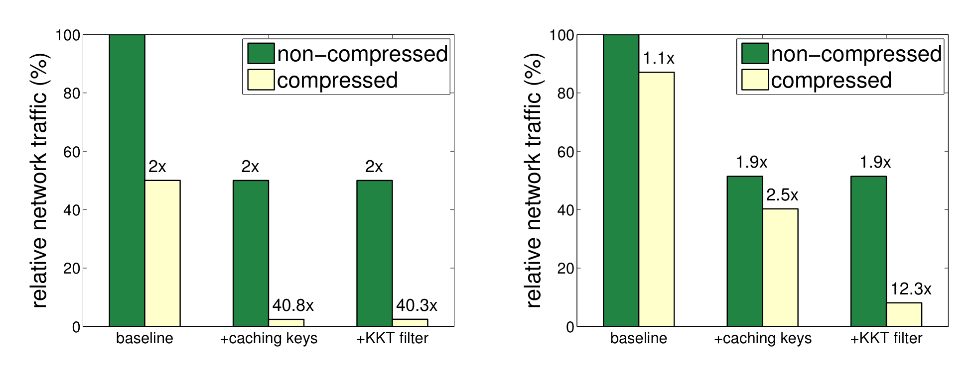
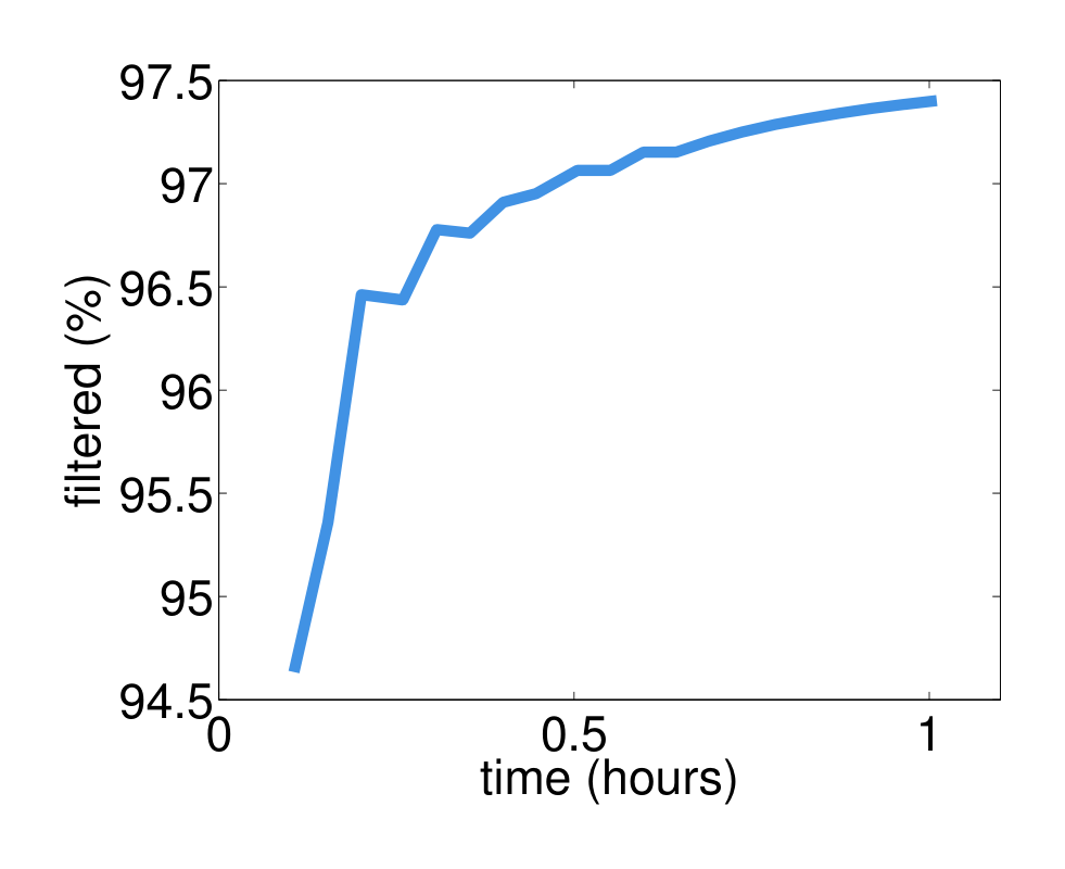
Next we evaluate the reduction of network traffic by each system components. Figure 11 shows the results for servers and workers. As can be seen, allowing the senders and receivers to cache the keys can save near 50% traffic. This is because both key (int64) and value (double) are of the same size, and the key set is not changed during optimization. In addition, data compression is effective for compressing the values for both servers (>20x) and workers when applying the KKT filter (>6x). The reason is twofold. First, the $\ell_1$ regularizer encourages a sparse model ($w$), so that most of values pulled from servers are 0. Second, the KKT filter forces a large portion of gradients sending to servers to be 0. This can be seen more clearly in Figure 12, which shows that more than 93% unique features are filtered by the KKT filter.

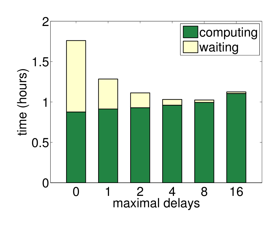
Finally, we analyze the bounded delay consistency model. The time decomposition of workers to achieve the same convergence criteria under different maximum allowed delay ($\tau$) is shown in Figure 13. As expected, the waiting time decreases when the allowed delay increases. Workers are 50% idle when using the sequential consistency model ($\tau = 0$), while the idle rate is reduced to 1.7% when $\tau$ is set to be 16. However, the computing time increases nearly linearly with $\tau$. Because the data inconsistency slows convergence, more iterations are needed to achieve the same convergence criteria. As a result, $\tau = 8$ is the best trade-off between algorithm convergence and system performance.

5.2 Latent Dirichlet Allocation

Problem and Data: To demonstrate the versatility of our approach, we applied the same parameter server architecture to the problem of modeling user interests based upon which domains appear in the URLs they click on in search results. We collected search log data containing 5 billion unique user identifiers and evaluated the model for the 5 million most frequently clicked domains in the result set. We ran the algorithm using 800 workers and 200 servers and 5000 workers and 1000 servers respectively. The machines had 10 physical cores, 128GB DRAM, and at least 10 Gb/s of network connectivity. We again shared the cluster with production jobs running concurrently.

Algorithm: We performed LDA using a combination of Stochastic Variational Methods [25], Collapsed Gibbs sampling [20] and distributed gradient descent. Here, gradients are aggregated asynchronously as they arrive from workers, along the lines of [1].

We divided the parameters in the model into local and global parameters. The local parameters (i.e. auxiliary metadata) are pertinent to a given user and they are streamed the from disk whenever we access a given user. The global parameters are shared among users and they are represented as (key,value) pairs to be stored using the parameter server. User data is sharded over workers. Each of them runs a set of computation threads to perform inference over its assigned users. We synchronize asynchronously to send and receive local updates to the server and receive new values of the global parameters.

To our knowledge, no other system (e.g., YahooLDA, Graphlab or Petuum) can handle this amount of data and model complexity for LDA, using up to 10 billion (5 million tokens and 2000 topics) shared parameters. The largest previously reported experiments [2] had under 100 million users active at any time, less than 100,000 tokens and under 1000 topics (2% the data, 1% the parameters).

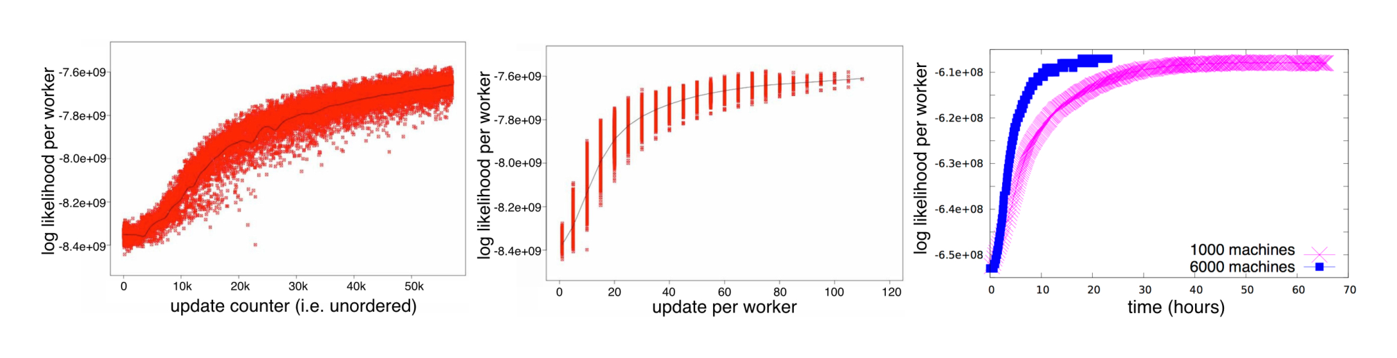
Results: To evaluate the quality of the inference algorithm we monitor how rapidly the training log-likelihood (measuring goodness of fit) converges. As can be seen in Figure 14, we observe an approximately 4x speedup in convergence when increasing the number of machines from 1000 to 6000. The stragglers observed in Figure 14 (leftmost) also illustrate the importance of having an architecture that can cope with performance variation across workers.

: Table 4: Example topics learned using LDA over the .5 billion dataset. Each topic represents a user interest.

\begin{tabular}{|l|l|}
\hline
Topic name & \# Top urls \\
\hline
Programming & stackoverflow.com w3schools.com cplusplus.com github.com tutorials- \\
& point.com jquery.com codeproject.com oracle.com qt-project.org bytes.com \\
& android.com mysql.com \\
\hline
Music & ultimate-guitar.com guitaretab.com 911tabs.com e-chords.com song- \\
& sterr.com chordify.net musicnotes.com ukulele-tabs.com \\
\hline
Baby Related & babycenter.com whattoexpect.com babycentre.co.uk circleofmoms.com \\
& thebump.com parents.com momtastic.com parenting.com americanpreg- \\
& nancy.org kidshealth.org \\
\hline
Strength Train- & bodybuilding.com muscleandfitness.com mensfitness.com menshealth.com \\
ing & t-nation.com livestrong.com muscleandstrength.com myfitnesspal.com elit- \\
& efitness.com crossfit.com steroid.com gnc.com askmen.com \\
\hline
\end{tabular}

5.3 Sketches

Problem and Data: We include sketches as part of our evaluation as a test of generality, because they operate very differently from machine learning algorithms. They typically observe a large number of writes of events coming from a streaming data source [11, 5].

We evaluate the time required to insert a streaming log of pageviews into an approximate structure that can efficiently track pageview counts for a large collection of web pages. We use the Wikipedia (and other Wiki projects) page view statistics as benchmark. Each entry is an unique key of a webpage with the corresponding number of requests served in a hour. From 12/2007 to 1/2014, there are 300 billion entries for more than 100 million unique keys. We run the parameter server with 90 virtual server nodes on 15 machines of a research cluster [40] (each has 64 cores and is connected by a 40Gb Ethernet).

Algorithm: Sketching algorithms efficiently store summaries of huge volumes of data so that approximate queries can be quickly answered. These algorithms are particularly important in streaming applications where data and queries arrive in real-time. Some of the highest-volume applications involve examples such as Cloudflare’s DDoS-prevention service, which must analyze page requests across its entire content delivery service architecture to identify likely DDoS targets and attackers. The volume of data logged in such applications considerably exceeds the capacity of a single machine. While a conventional approach might be to shard a workload across a key-value cluster such as Redis, these systems typically do not allow the user-defined aggregation semantics needed to implement approximate aggregation.

Algorithm 4 gives a brief overview of the CountMin sketch [11]. By design, the result of a query is an upper bound on the number of observed keys $x$. Splitting keys into ranges automatically allows us to parallelize the sketch. Unlike the two previous applications, the workers simply dispatch updates to the appropriate servers.

Algorithm 4 CountMin Sketch
Init: $M[i, j] = 0$ for $i \in \{1, \dots, n\}$ and $j \in \{1, \dots, k\}$.
Insert($x$)
1: for $i = 1$ to $k$ do
2:   $M[i, \text{hash}(i, x)] \leftarrow M[i, \text{hash}(i, x)] + 1$
Query($x$)
1: return $\min \{M[i, \text{hash}(i, x)] \text{ for } 1 \leq i \leq k\}$

Results: The system achieves very high insert rates, which are shown in Table 5. It performs well for two reasons: First, bulk communication reduces the communication cost. Second, message compression reduces the average (key,value) size to around 50 bits. Importantly, when we terminated a server node during the insertion, the parameter server was able to recover the failed node within 1 second, making our system well equipped for realtime.

: Table 5: Results of distributed CountMin.

\begin{tabular}{|l|l|}
\hline
Peak inserts per second & 1.3 billion \\
Average inserts per second & 1.1 billion \\
Peak net bandwidth per machine & 4.37 GBit/s \\
Time to recover a failed node & 0.8 second \\
\hline
\end{tabular}

6 Summary and Discussion

Section Summary: This section summarizes a parameter server framework designed to handle distributed machine learning tasks by allowing shared parameters to act like simple local data structures for computations with training information. The framework is user-friendly and efficient, using asynchronous communication and adjustable consistency options to speed up results while supporting scalability and error recovery for long-term use. Experiments on large real-world datasets with billions of data points confirm its effectiveness, positioning it as a key tool for advanced machine learning, with open-source code available online.

We described a parameter server framework to solve distributed machine learning problems. This framework is easy to use: Globally shared parameters can be used as local sparse vectors or matrices to perform linear algebra operations with local training data. It is efficient: All communication is asynchronous. Flexible consistentcy models are supported to balance the trade-off between system efficiency and fast algorithm convergence rate. Furthermore, it provides elastic scalability and fault tolerance, aiming for stable long term deployment. Finally, we show experiments for several challenging tasks on real datasets with billions of variables to demonstrate its efficiency. We believe that this third generation parameter server is an important building block for scalable machine learning. The codes are available at parameterserver.org.

Acknowledgments: This work was supported in part by gifts and/or machine time from Google, Amazon, Baidu, PRObE, and Microsoft; by NSF award 1409802; and by the Intel Science and Technology Center for Cloud Computing. We are grateful to our reviewers and colleagues for their comments on earlier versions of this paper.

References

Section Summary: This section lists over 30 references cited in a technical document, primarily focusing on research papers, books, and software tools related to machine learning, data processing, and distributed computing systems. It includes influential works on scalable inference in latent variable models, distributed deep networks, probabilistic graphical models, and frameworks like MapReduce, Hadoop, and parameter servers, authored by prominent researchers such as David Blei, Jeff Dean, and Andrew Ng. The sources span conferences, journals, theses, and project websites from 1988 to 2014, providing foundational support for topics in large-scale data analysis and algorithm optimization.

[1] A. Ahmed, M. Aly, J. Gonzalez, S. Narayanamurthy, and A. J. Smola. Scalable inference in latent variable models. In Proceedings of The 5th ACM International Conference on Web Search and Data Mining (WSDM), 2012.

[2] A. Ahmed, Y. Low, M. Aly, V. Josifovski, and A. J. Smola. Scalable inference of dynamic user interests for behavioural targeting. In Knowledge Discovery and Data Mining, 2011.

[3] E. Anderson, Z. Bai, C. Bischof, J. Demmel, J. Dongarra, J. Du Croz, A. Greenbaum, S. Hammarling, A. McKenney, S. Ostrouchov, and D. Sorensen. LAPACK Users’ Guide. SIAM, Philadelphia, second edition, 1995.

[4] Apache Foundation. Mahout project, 2012. http://mahout.apache.org.

[5] R. Berinde, G. Cormode, P. Indyk, and M.J. Strauss. Space-optimal heavy hitters with strong error bounds. In J. Paredaens and J. Su, editors, Proceedings of the TwentyEigth ACM SIGMOD-SIGACT-SIGART Symposium on Principles of Database Systems, PODS, pages 157–166. ACM, 2009.

[6] C. Bishop. Pattern Recognition and Machine Learning. Springer, 2006.

[7] D. Blei, A. Ng, and M. Jordan. Latent Dirichlet allocation. Journal of Machine Learning Research, 3:993–1022, January 2003.

[8] J. Byers, J. Considine, and M. Mitzenmacher. Simple load balancing for distributed hash tables. In Peer-to-peer systems II, pages 80–87. Springer, 2003.

[9] K. Canini. Sibyl: A system for large scale supervised machine learning. Technical Talk, 2012.

[10] B.-G. Chun, T. Condie, C. Curino, C. Douglas, S. Matusevych, B. Myers, S. Narayanamurthy, R. Ramakrishnan, S. Rao, J. Rosen, R. Sears, and M. Weimer. Reef: Retainable evaluator execution framework. Proceedings of the VLDB Endowment, 6(12):1370–1373, 2013.

[11] G. Cormode and S. Muthukrishnan. Summarizing and mining skewed data streams. In SDM, 2005.

[12] W. Dai, J. Wei, X. Zheng, J. K. Kim, S. Lee, J. Yin, Q. Ho, and E. P. Xing. Petuum: A framework for iterative-convergent distributed ml. arXiv preprint arXiv:1312.7651, 2013.

[13] J. Dean, G. Corrado, R. Monga, K. Chen, M. Devin, Q. Le, M. Mao, M. Ranzato, A. Senior, P. Tucker, K. Yang, and A. Ng. Large scale distributed deep networks. In Neural Information Processing Systems, 2012.

[14] J. Dean and S. Ghemawat. MapReduce: simplified data processing on large clusters. CACM, 51(1):107–113, 2008.

[15] G. DeCandia, D. Hastorun, M. Jampani, G. Kakulapati, A. Lakshman, A. Pilchin, S. Sivasubramanian, P. Vosshall, and W. Vogels. Dynamo: Amazon’s highly available key-value store. In T. C. Bressoud and M. F. Kaashoek, editors, Symposium on Operating Systems Principles, pages 205–220. ACM, 2007.

[16] J. J. Dongarra, J. Du Croz, S. Hammarling, and R. J. Hanson. An extended set of fortran basic linear algebra subprograms. ACM Transactions on Mathematical Software, 14:18–32, 1988.

[17] The Apache Software Foundation. Apache hadoop nextgen mapreduce (yarn). http://hadoop.apache.org/.

[18] The Apache Software Foundation. Apache hadoop, 2009. http://hadoop.apache.org/core/.

[19] F. Girosi, M. Jones, and T. Poggio. Priors, stabilizers and basis functions: From regularization to radial, tensor and additive splines. A.I. Memo 1430, Artificial Intelligence Laboratory, Massachusetts Institute of Technology, 1993.

[20] T.L. Griffiths and M. Steyvers. Finding scientific topics. Proceedings of the National Academy of Sciences, 101:5228–5235, 2004.

[21] S. H. Gunderson. Snappy: A fast compressor/decompressor. https://code.google.com/p/snappy/.

[22] T. Hastie, R. Tibshirani, and J. Friedman. The Elements of Statistical Learning. Springer, New York, 2 edition, 2009.

[23] B. Hindman, A. Konwinski, M. Zaharia, A. Ghodsi, A. D. Joseph, R. Katz, S. Shenker, and I. Stoica. Mesos: A platform for fine-grained resource sharing in the data center. In Proceedings of the 8th USENIX conference on Networked systems design and implementation, pages 22–22, 2011.

[24] Q. Ho, J. Cipar, H. Cui, S. Lee, J. Kim, P. Gibbons, G. Gibson, G. Ganger, and E. Xing. More effective distributed ml via a stale synchronous parallel parameter server. In NIPS, 2013.

[25] M. Hoffman, D. M. Blei, C. Wang, and J. Paisley. Stochastic variational inference. In International Conference on Machine Learning, 2012.

[26] W. Karush. Minima of functions of several variables with inequalities as side constraints. Master’s thesis, Dept. of Mathematics, Univ. of Chicago, 1939.

[27] L. Kim. How many ads does Google serve in a day?, 2012. http://goo.gl/oIidXO.

[28] D. Koller and N. Friedman. Probabilistic Graphical Models: Principles and Techniques. MIT Press, 2009.

[29] T. Kraska, A. Talwalkar, J. C. Duchi, R. Griffith, M. J. Franklin, and M. I. Jordan. Mlbase: A distributed machine-learning system. In CIDR, 2013.

[30] L. Lamport. Paxos made simple. ACM Sigact News, 32(4):18–25, 2001.

[31] M. Li, D. G. Andersen, and A. J. Smola. Distributed delayed proximal gradient methods. In NIPS Workshop on Optimization for Machine Learning, 2013.

[32] M. Li, D. G. Andersen, and A. J. Smola. Communication Efficient Distributed Machine Learning with the Parameter Server. In Neural Information Processing Systems, 2014.

[33] M. Li, L. Zhou, Z. Yang, A. Li, F. Xia, D.G. Andersen, and A. J. Smola. Parameter server for distributed machine learning. In Big Learning NIPS Workshop, 2013.

[34] Y. Low, J. Gonzalez, A. Kyrola, D. Bickson, C. Guestrin, and J. M. Hellerstein. Distributed Graphlab: A framework for machine learning and data mining in the cloud. In PVLDB, 2012.

[35] H. B. McMahan, G. Holt, D. Sculley, M. Young, D. Ebner, J. Grady, L. Nie, T. Phillips, E. Davydov, and D. Golovin. Ad click prediction: a view from the trenches. In KDD, 2013.

[36] K. P. Murphy. Machine learning: a probabilistic perspective. MIT Press, 2012.

[37] D. G. Murray, F. McSherry, R. Isaacs, M. Isard, P. Barham, and M. Abadi. Naiad: a timely dataflow system. In Proceedings of the Twenty-Fourth ACM Symposium on Operating Systems Principles, pages 439–455. ACM, 2013.

[38] A. Phanishayee, D. G. Andersen, H. Pucha, A. Povzner, and W. Belluomini. Flex-KV: Enabling high-performance and flexible KV systems. In Proceedings of the 2012 workshop on Management of big data systems, pages 19–24. ACM, 2012.

[39] R. Power and J. Li. Piccolo: Building fast, distributed programs with partitioned tables. In R. H. Arpaci-Dusseau and B. Chen, editors, Operating Systems Design and Implementation, OSDI, pages 293–306. USENIX Association, 2010.

[40] PRObE Project. Parallel Reconfigurable Observational Environment. https://www.nmc-probe.org/wiki/Machines:Susitna,

[41] A. Rowstron and P. Druschel. Pastry: Scalable, decentralized object location and routing for large-scale peer-topeer systems. In IFIP/ACM International Conference on Distributed Systems Platforms (Middleware), pages 329– 350, Heidelberg, Germany, November 2001.

[42] B. Scholkopf and A. J. Smola. Learning with Kernels. MIT Press, Cambridge, MA, 2002.

[43] A. J. Smola and S. Narayanamurthy. An architecture for parallel topic models. In Very Large Databases (VLDB), 2010.

[44] E. Sparks, A. Talwalkar, V. Smith, J. Kottalam, X. Pan, J. Gonzalez, M. J. Franklin, M. I. Jordan, and T. Kraska. Mli: An api for distributed machine learning. 2013.

[45] I. Stoica, R. Morris, D. Karger, M. F. Kaashoek, and H. Balakrishnan. Chord: A scalable peer-to-peer lookup service for internet applications. ACM SIGCOMM Computer Communication Review, 31(4):149–160, 2001.

[46] C.H. Teo, Q. Le, A. J. Smola, and S. V. N. Vishwanathan. A scalable modular convex solver for regularized risk minimization. In Proc. ACM Conf. Knowledge Discovery and Data Mining (KDD). ACM, 2007.

[47] R. van Renesse and F. B. Schneider. Chain replication for supporting high throughput and availability. In OSDI, volume 4, pages 91–104, 2004.

[48] V. Vapnik. The Nature of Statistical Learning Theory. Springer, New York, 1995.

[49] R.C. Whaley, A. Petitet, and J.J. Dongarra. Automated empirical optimization of software and the ATLAS project. Parallel Computing, 27(1–2):3–35, 2001.

[50] M. Zaharia, M. Chowdhury, T. Das, A. Dave, J. M. Ma, M. McCauley, M. J. Franklin, S. Shenker, and I. Stoica. Fast and interactive analytics over Hadoop data with Spark. USENIX ;login:, 37(4):45–51, August 2012.