Deep & Cross Network for Ad Click Predictions

Ruoxi Wang Stanford University Stanford, CA [email protected]

Bin Fu Google Inc. New York, NY [email protected]

Gang Fu Google Inc. New York, NY [email protected]

Mingliang Wang Google Inc. New York, NY [email protected]

Abstract

Feature engineering has been the key to the success of many prediction models. However, the process is nontrivial and often requires manual feature engineering or exhaustive searching. DNNs are able to automatically learn feature interactions; however, they generate all the interactions implicitly, and are not necessarily efficient in learning all types of cross features. In this paper, we propose the Deep & Cross Network (DCN) which keeps the benefits of a DNN model, and beyond that, it introduces a novel cross network that is more efficient in learning certain bounded-degree feature interactions. In particular, DCN explicitly applies feature crossing at each layer, requires no manual feature engineering, and adds negligible extra complexity to the DNN model. Our experimental results have demonstrated its superiority over the state-of-art algorithms on the CTR prediction dataset and dense classification dataset, in terms of both model accuracy and memory usage.

Executive Summary: The document addresses click-through rate (CTR) prediction for large-scale online advertising, where revenue depends on accurate forecasts of user clicks. Data is high-dimensional and sparse, consisting mostly of categorical features. Linear models such as logistic regression have long dominated because they scale well, yet they require costly manual feature engineering or exhaustive search to capture useful feature interactions; standard deep neural networks can learn interactions automatically but do so implicitly, often at high parameter cost and without guaranteed efficiency for bounded-degree crossings.

The paper therefore introduces the Deep & Cross Network (DCN). Its goal is to combine the nonlinear capacity of a DNN with an explicit, parameter-efficient cross network that automatically forms higher-order feature interactions whose maximum degree is controlled by network depth.

The model begins with an embedding layer that converts sparse categorical inputs into dense vectors. These are processed in parallel by a cross network (each layer multiplies the original input vector by the previous layer output and adds a residual) and a conventional fully-connected DNN. Outputs are concatenated and passed through a final logistic layer. Training uses standard mini-batch Adam optimization on the log-loss. Experiments compare DCN with logistic regression, factorization machines, Wide & Deep, Deep Crossing, and a pure DNN baseline, using the 41-million-record Criteo display-ads data set (first six days for training, seventh day for validation and test) plus two UCI classification sets.

DCN records the lowest test log-loss (0.4419) on Criteo while using roughly 40 % of the parameters required by the best pure DNN. Under identical memory budgets it consistently outperforms the DNN baseline; the advantage is largest at modest parameter counts and remains material even when the DNN is given several times more capacity. Accuracy gains appear after the first cross layer and continue, though diminishingly, with added depth. The same pattern holds on the non-CTR data sets, where DCN again matches or exceeds DNN accuracy at half the memory.

These results indicate that explicit, low-degree feature crossing is both learnable and cheaper than implicit learning inside a large DNN. The practical payoff is higher prediction accuracy at lower memory and compute cost, which matters directly for revenue in CPC advertising and for serving latency at web scale.

The authors recommend replacing or augmenting existing DNN pipelines with cross layers when memory is constrained or when domain knowledge suggests low-to-moderate-order interactions dominate. Further work is needed on very deep cross networks, on systematic integration with other architectures, and on theoretical characterization of the function class the cross network can efficiently approximate. Results rely on grid search over a modest range of depths and widths and on early stopping; therefore new data distributions or substantially larger models should be re-tuned before production deployment.

1. Introduction

Section Summary: Click-through rate prediction is essential for revenue in online advertising under pay-per-click models, yet the vast, sparse, and categorical nature of web data makes it difficult for simple linear models to discover useful combinations of features without laborious manual engineering. The paper introduces a Deep & Cross Network that pairs a novel cross network—designed to automatically build higher-order feature interactions layer by layer—with a conventional deep neural network, capturing predictive patterns more explicitly and efficiently than either component alone. Experiments show this hybrid yields state-of-the-art accuracy on large CTR datasets while using nearly an order of magnitude fewer parameters than a deep network by itself.

Click-through rate (CTR) prediction is a large-scale problem that is essential to multi-billion dollar online advertising industry. In the advertising industry, advertisers pay publishers to display their ads on publishers'sites. One popular payment model is the cost-per-click (CPC) model, where advertisers are charged only when a click occurs. As a consequence, a publisher's revenue relies heavily on the ability to predict CTR accurately.

Identifying frequently predictive features and at the same time exploring unseen or rare cross features is the key to making good predictions. However, data for Web-scale recommender systems is mostly discrete and categorical, leading to a large and sparse feature space that is challenging for feature exploration. This has limited most large-scale systems to linear models such as logistic regression.

Linear models [1] are simple, interpretable and easy to scale; however, they are limited in their expressive power. Cross features, on the other hand, have been shown to be significant in improving the models' expressiveness. Unfortunately, it often requires manual feature engineering or exhaustive search to identify such features; moreover, generalizing to unseen feature interactions is difficult.

In this paper, we aim to avoid task-specific feature engineering by introducing a novel neural network structure – a cross network – that explicitly applies feature crossing in an automatic fashion. The cross network consists of multiple layers, where the highest-degree of interactions are provably determined by layer depth. Each layer produces higher-order interactions based on existing ones, and keeps the interactions from previous layers. We train the cross network jointly with a deep neural network (DNN) [2, 3]. DNN has the promise to capture very complex interactions across features; however, compared to our cross network it requires nearly an order of magnitude more parameters, is unable to form cross features explicitly, and may fail to efficiently learn some types of feature interactions. Jointly training the cross and DNN components together, however, efficiently captures predictive feature interactions, and delivers state-of-the-art performance on the Criteo CTR dataset.

1.1 Related Work

Due to the dramatic increase in size and dimensionality of datasets, a number of methods have been proposed to avoid extensive task-specific feature engineering, mostly based on embedding techniques and neural networks.

Factorization machines (FMs) [4, 5] project sparse features onto low-dimensional dense vectors and learn feature interactions from vector inner products. Field-aware factorization machines (FFMs) [6, 7] further allow each feature to learn several vectors where each vector is associated with a field. Regrettably, the shallow structures of FMs and FFMs limit their representative power. There have been work extending FMs to higher orders [8, 9], but one downside lies in their large number of parameters which yields undesirable computational cost. Deep neural networks (DNN) are able to learn non-trivial high-degree feature interactions due to embedding vectors and nonlinear activation functions. The recent success of the Residual Network [10] has enabled training of very deep networks. Deep Crossing [11] extends residual networks and achieves automatic feature learning by stacking all types of inputs.

The remarkable success of deep learning has elicited theoretical analyses on its representative power. There has been research [12, 13] showing that DNNs are able to approximate an arbitrary function under certain smoothness assumptions to an arbitrary accuracy, given sufficiently many hidden units or hidden layers. Moreover, in practice, it has been found that DNNs work well with a feasible number of parameters. One key reason is that most functions of practical interest are not arbitrary.

Yet one remaining question is whether DNNs are indeed the most efficient ones in representing such functions of practical interest. In the Kaggle^3 competition, the manually crafted features in many winning solutions are low-degree, in an explicit format and effective. The features learned by DNNs, on the other hand, are implicit and highly nonlinear. This has shed light on designing a model that is able to learn bounded-degree feature interactions more efficiently and explicitly than a universal DNN.

The wide-and-deep [14] is a model in this spirit. It takes cross features as inputs to a linear model, and jointly trains the linear model with a DNN model. However, the success of wide-and-deep hinges on a proper choice of cross features, an exponential problem for which there is yet no clear efficient method.

1.2 Main Contributions

In this paper, we propose the Deep & Cross Network (DCN) model that enables Web-scale automatic feature learning with both sparse and dense inputs. DCN efficiently captures effective feature interactions of bounded degrees, learns highly nonlinear interactions, requires no manual feature engineering or exhaustive searching, and has low computational cost.

The main contributions of the paper include:

• We propose a novel cross network that explicitly applies feature crossing at each layer, efficiently learns predictive cross features of bounded degrees, and requires no manual feature engineering or exhaustive searching.
• The cross network is simple yet effective. By design, the highest polynomial degree increases at each layer and is determined by layer depth. The network consists of all the cross terms of degree up to the highest, with their coefficients all different.
• The cross network is memory efficient, and easy to implement.
• Our experimental results have demonstrated that with a cross network, DCN has lower logloss than a DNN with nearly an order of magnitude fewer number of parameters.

The paper is organized as follows: Section 2 describes the architecture of the Deep & Cross Network. Section 3 analyzes the cross network in detail. Section 4 shows the experimental results.

2. Deep & Cross Network (DCN)

Section Summary: The Deep & Cross Network (DCN) is a neural network architecture designed for large-scale recommendation tasks that processes input features through an initial embedding layer to convert high-dimensional categorical data into compact vectors, which are then stacked with dense features. These processed inputs feed in parallel into a cross network that explicitly builds higher-order feature interactions through simple layered operations and a conventional deep network that captures complex nonlinear patterns. The outputs of the two parallel networks are finally concatenated in a combination layer to produce the model's prediction.

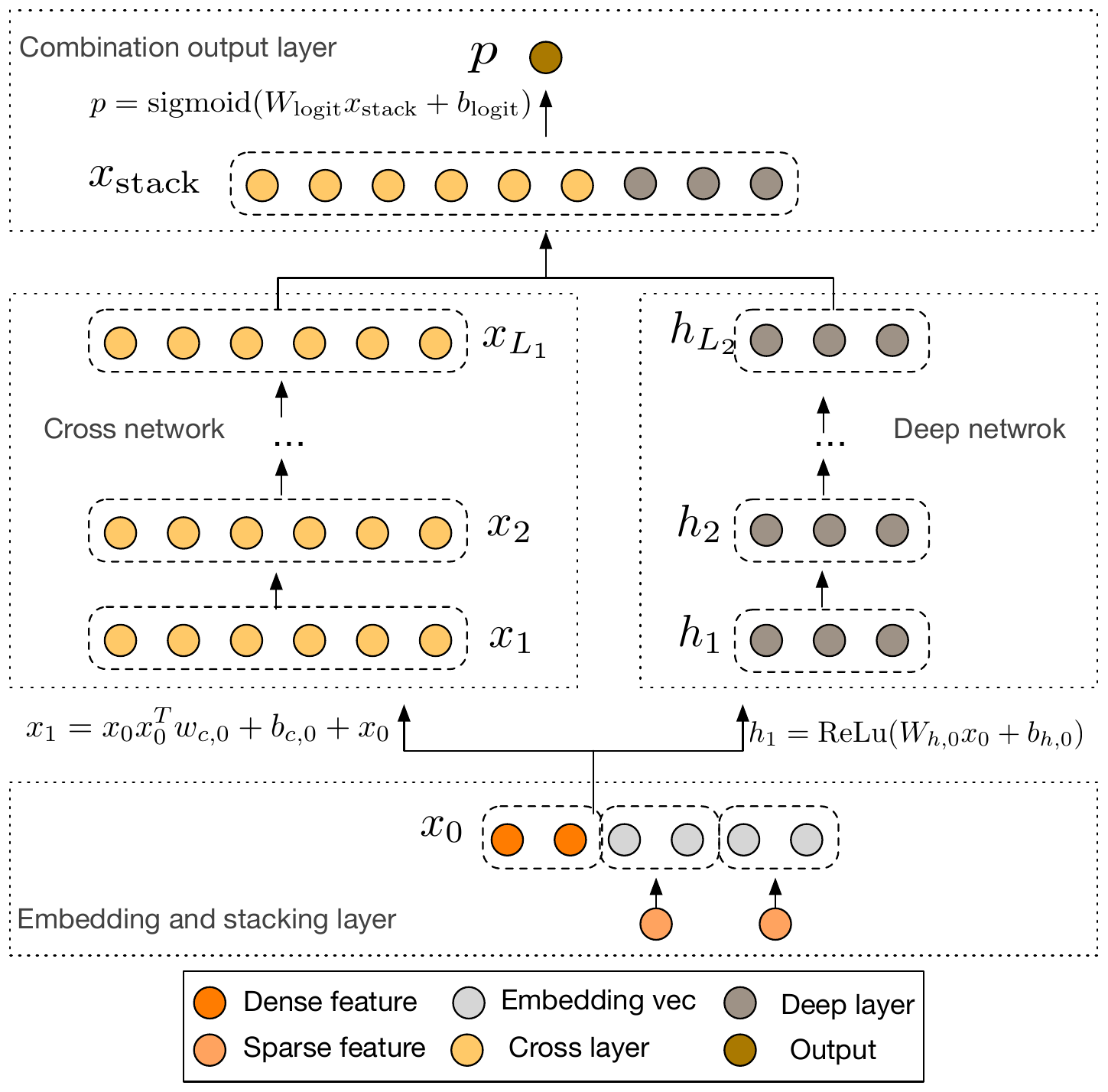
In this section we describe the architecture of Deep & Cross Network (DCN) models. A DCN model starts with an embedding and stacking layer, followed by a cross network and a deep network in parallel. These in turn are followed by a final combination layer which combines the outputs from the two networks. The complete DCN model is depicted in Figure 1.

2.1 Embedding and Stacking Layer

We consider input data with sparse and dense features. In Web-scale recommender systems such as CTR prediction, the inputs are mostly categorical features, e.g. "country=usa". Such features are often encoded as one-hot vectors e.g. "[0, 1, 0]"; however, this often leads to excessively high-dimensional feature spaces for large vocabularies.

To reduce the dimensionality, we employ an embedding procedure to transform these binary features into dense vectors of real values (commonly called embedding vectors):

$ {\bf x}{\text{embed}, i} = W{\text{embed}, i}{\bf x}_i, $

where ${\bf x}_{\text{embed}, i}$ is the embedding vector, ${\bf x}i$ is the binary input in the $i$-th category, and $W{\text{embed}, i} \in \mathbb{R}^{n_e \times n_v}$ is the corresponding embedding matrix that will be optimized together with other parameters in the network, and $n_e, n_v$ are the embedding size and vocabulary size, respectively.

In the end, we stack the embedding vectors, along with the normalized dense features ${\bf x}_{\text{dense}}$, into one vector:

$ {\bf x}0 = \left[{\bf x}{\text{embed}, 1}^T, \ldots, {\bf x}{\text{embed}, k}^T, {\bf x}{\text{dense}}^T\right], $

and feed ${\bf x}_0$ to the network.

2.2 Cross Network

The key idea of our novel cross network is to apply explicit feature crossing in an efficient way. The cross network is composed of cross layers, with each layer having the following formula:

$ {\bf x}_{l+1} = {\bf x}_0 {\bf x}_l^T {\bf w}_l + {\bf b}_l +{\bf x}_l = f({\bf x}_l, {\bf w}_l, {\bf b}_l) +{\bf x}_l,\tag{1} $

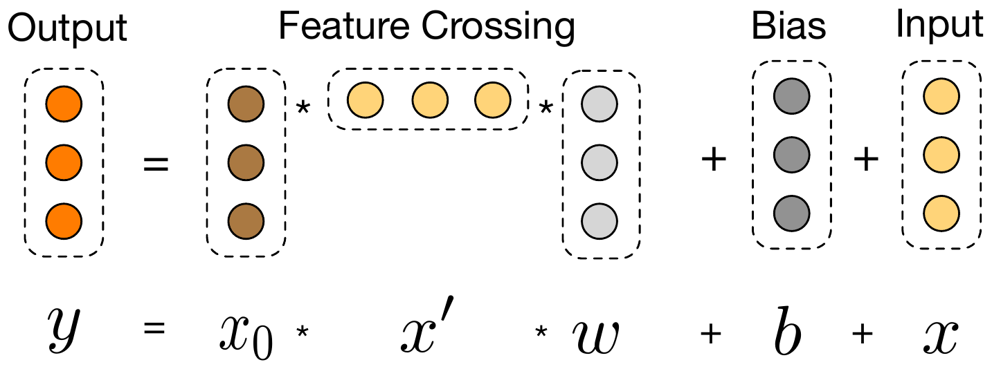
where ${\bf x}l, {\bf x}{l+1} \in \mathbb{R}^{d}$ are column vectors denoting the outputs from the $l$-th and $(l+1)$-th cross layers, respectively; ${\bf w}_l, {\bf b}l \in \mathbb{R}^{d}$ are the weight and bias parameters of the $l$-th layer. Each cross layer adds back its input after a feature crossing $f$, and the mapping function $f: \mathbb{R}^{d} \mapsto \mathbb{R}^{d}$ fits the residual of ${\bf x}{l+1} -{\bf x}_l$. A visualization of one cross layer is shown in Figure 2.

High-degree Interaction Across Features. The special structure of the cross network causes the degree of cross features to grow with layer depth. The highest polynomial degree (in terms of input ${\bf x}_0$) for an $l$-layer cross network is $l+1$. In fact, the cross network comprises all the cross terms $x_1^{\alpha_1}x_2^{\alpha_2}\ldots x_d^{\alpha_d}$ of degree from 1 to $l+1$. Detailed analysis is in Section 3.

Complexity Analysis. Let $L_c$ denote the number of cross layers, and $d$ denote the input dimension. Then, the number of parameters involved in the cross network is

$ d \times L_c \times 2. $

The time and space complexity of a cross network are linear in input dimension. Therefore, a cross network introduces negligible complexity compared to its deep counterpart, keeping the overall complexity for DCN at the same level as that of a traditional DNN. This efficiency benefits from the rank-one property of ${\bf x}_0 {\bf x}_l^T$, which enables us to generate all cross terms without computing or storing the entire matrix.

The small number of parameters of the cross network has limited the model capacity. To capture highly nonlinear interactions, we introduce a deep network in parallel.

2.3 Deep Network

The deep network is a fully-connected feed-forward neural network, with each deep layer having the following formula:

$ {\bf h}_{l+1} = f(W_l {\bf h}_l + {\bf b}_l), $

where ${\bf h}l \in \mathbb{R}^{n_l}, {\bf h}{l+1}\in \mathbb{R}^{n_{l+1}}$ are the $l$-th and $(l+1)$-th hidden layer, respectively; $W_l \in \mathbb{R}^{n_{l+1} \times n_l}, {\bf b}l \in \mathbb{R}^{n{l+1}}$ are parameters for the $l$-th deep layer; and $f(\cdot)$ is the ReLU function.

Complexity Analysis. For simplicity, we assume all the deep layers are of equal size. Let $L_d$ denote the number of deep layers and $m$ denote the deep layer size. Then, the number of parameters in the deep network is

$ d \times m + m + (m^2+ m) \times (L_d-1). $

2.4 Combination Layer

The combination layer concatenates the outputs from two networks and feed the concatenated vector into a standard logits layer.

The following is the formula for a two-class classification problem:

$ p = \sigma\left([{\bf x}{L_1}^T, {\bf h}{L_2}^T] {\bf w}_{\text{logits}} \right),\tag{2} $

where ${\bf x}{L_1} \in \mathbb{R}^{d}, {\bf h}{L_2} \in \mathbb{R}^{m}$ are the outputs from the cross network and deep network, respectively, ${\bf w}_{\text{logits}} \in \mathbb{R}^{(d + m)}$ is the weight vector for the combination layer, and $\sigma(x) = 1/(1+\exp(-x))$.

The loss function is the log loss along with a regularization term,

$ \begin{split} \text{loss} = &-\frac{1}{N} \sum_{i = 1}^N y_i \log(p_i) + (1 - y_i) \log(1 - p_i) + \lambda \sum_l | {\bf w}_l|^2, \end{split} $

where $p_i$ 's are the probabilities computed from Equation 2, $y_i$ 's are the true labels, $N$ is the total number of inputs, and $\lambda$ is the $L_2$ regularization parameter.

We jointly train both networks, as this allows each individual network to be aware of the others during the training.

3. Cross Network Analysis

Section Summary: The cross network in DCN is examined from three angles to explain its strong performance. It can approximate high-degree multivariate polynomials using only a linear number of parameters, extends the parameter-sharing approach of factorization machines to deeper layers and higher-order feature interactions for better generalization on sparse data, and performs an efficient linear-cost projection of all pairwise feature crosses back into the original input dimension. Together these properties let the model capture rich interactions without the usual explosion in parameters or compute.

In this section, we analyze the cross network of DCN for the purpose of understanding its effectiveness. We offer three perspectives: polynomial approximation, generalization to FMs, and efficient projection. For simplicity, we assume ${\bf b}_i = 0$.

Notations. Let the $i$-th element in ${\bf w}j$ be $w{j}^{(i)}$. For multi-index ${\bm \alpha} = [\alpha_1, \cdot s, \alpha_d] \in \mathbb{N}^d$ and ${\bf x} = [x_1, \cdot s, x_d] \in \mathbb{R}^d$, we define $| {\bm \alpha}| = \sum_{i=1}^d \alpha_i$.

Terminology. The degree of a cross term (monomial) $x_1^{\alpha_1}x_2^{\alpha_2}\cdot s x_d^{\alpha_d}$ is defined by $| {\bm \alpha}|$. The degree of a polynomial is defined by the highest degree of its terms.

3.1 Polynomial Approximation

By the Weierstrass approximation theorem [15], any function under certain smoothness assumption can be approximated by a polynomial to an arbitrary accuracy. Therefore, we analyze the cross network from the perspective of polynomial approximation. In particular, the cross network approximates the polynomial class of the same degree in a way that is efficient, expressive and generalizes better to real-world datasets.

We study in detail the approximation of a cross network to the polynomial class of the same degree. Let us denote by $P_n({\bf x})$ the multivariate polynomial class of degree $n$:

$ P_{n}({\bf x}) = \biggl{\sum_{{\bm \alpha}} w_{{\bm \alpha}} x_1^{\alpha_1}x_2^{\alpha_2}\ldots x_d^{\alpha_d} \mathrel{\bigg|} 0 \le | {\bm \alpha}| \le n, {\bm \alpha} \in \mathbb{N}^d \biggr}. $

Each polynomial in this class has $O(d^n)$ coefficients. We show that, with only $O(d)$ parameters, the cross network contains all the cross terms occurring in the polynomial of the same degree, with each term's coefficient distinct from each other.

########## caption="Theorem 1"

Consider an $l$-layer cross network with the $i+1$-th layer defined as ${\bf x}{i+1} = {\bf x}{0}{\bf x}{i}^T {\bf w}{i} +{\bf x}_{i}$. Let the input to the network be ${\bf x}_0 = [x_1, x_2, \ldots, x_d]^T$, the output be $g_l({\bf x}_0) = {\bf x}_l^T {\bf w}_l$, and the parameters be ${\bf w}_i, {\bf b}_i \in \mathbb{R}^d$. Then, the multivariate polynomial $g_l({\bf x}_0)$ reproduces polynomials in the following class:

$ \biggl{\sum_{{\bm \alpha}} c_{{\bm \alpha}}({\bf w}_0, \ldots, {\bf w}_l) x_1^{\alpha_1}x_2^{\alpha_2}\ldots x_d^{\alpha_d} \mathrel{\bigg|} 0 \le | {\bm \alpha}| \le l+1, {\bm \alpha} \in \mathbb{N}^d \biggr}, $

where $c_{{\bm \alpha}} = M_{{\bm \alpha}}\sum_{{\bf i} \in B_{\bm \alpha}}\sum_{{\bf j} \in P_{\bm \alpha} } \prod_{k=1}^{| {\bm \alpha}|} w_{i_k}^{(j_k)}$, $M_{\bm \alpha}$ is a constant independent of ${\bf w}i$ 's, ${\bf i} = [i_1, \ldots, i{| {\bm \alpha}|}]$ and ${\bf j} = [j_1, \ldots, j_{| {\bm \alpha}|}]$ are multi-indices, $B_{{\bm \alpha}} = \bigl{{\bf y} \in {0, 1, \cdot s, l}^{| {\bm \alpha}|} \mathrel{\big|} y_i < y_j \wedge y_{| {\bm \alpha}|} = l\bigr}$, and $P_{\bm \alpha}$ is the set of all the permutations of the indices $(\underbrace{1, \cdot s, 1}{\alpha_1 , \text{times}} \cdot s \underbrace{d, \cdot s, d}{\alpha_d, \text{times}})$.

The proof of Theorem 1 is in the Appendix. Let us give an example. Consider the coefficient $c_{{\bm \alpha}}$ for $x_1x_2x_3$ with ${\bm \alpha} = (1, 1, 1, 0, \ldots, 0)$. Up to some constant, when $l=2$, $c_{\bm \alpha} = \sum_{i, j, k \in P_{\bm \alpha}} w_0^{(i)}w_1^{(j)}w_2^{(k)}$; when $l=3$, $c_{\bm \alpha} = \sum_{i, j, k \in P_{\bm \alpha}} w_0^{(i)}w_1^{(j)}w_3^{(k)} + w_0^{(i)}w_2^{(j)}w_3^{(k)} + w_1^{(i)}w_2^{(j)}w_3^{(k)}$.

3.2 Generalization of FMs

The cross network shares the spirit of parameter sharing as the FM model and further extends it to a deeper structure.

In a FM model, feature $x_i$ is associated with a weight vector ${\bf v}i$, and the weight of cross term $x_ix_j$ is computed by $\langle {\bf v}i, {\bf v}j\rangle$. In DCN, $x_i$ is associated with scalars ${w_k^{(i)}}{k=1}^l$, and the weight of $x_ix_j$ is the multiplications of parameters from the sets ${w{k}^{(i)}}{k=0}^l$ and ${w_{k}^{(j)}}_{k=0}^l$. Both models have each feature learned some parameters independent from other features, and the weight of a cross term is a certain combination of corresponding parameters.

Parameter sharing not only makes the model more efficient, but also enables the model to generalize to unseen feature interactions and be more robust to noise. For example, take datasets with sparse features. If two binary features $x_i$ and $x_j$ rarely or never co-occur in the training data, i.e., $x_i \neq 0 \wedge x_j \neq 0$, then the learned weight of $x_ix_j$ would carry no meaningful information for prediction.

The FM is a shallow structure and is limited to representing cross terms of degree 2. DCN, in contrast, is able to construct all the cross terms $x_1^{\alpha_1}x_2^{\alpha_2}\ldots x_d^{\alpha_d}$ with degree $| {\bm \alpha}|$ bounded by some constant determined by layer depth, as claimed in Theorem 1. Therefore, the cross network extends the idea of parameter sharing from a single layer to multiple layers and high-degree cross-terms. Note that different from the higher-order FMs, the number of parameters in a cross network only grows linearly with the input dimension.

3.3 Efficient Projection

Each cross layer projects all the pairwise interactions between ${\bf x}_0$ and ${\bf x}_l$, in an efficient manner, back to the input's dimension.

Consider $\tilde {\bf x} \in \mathbb{R}^{d}$ as the input to a cross layer. The cross layer first implicitly constructs $d^2$ pairwise interactions $x_i\tilde{x}_j$, and then implicitly projects them back to dimension $d$ in a memory-efficient way. A direct approach, however, comes with a cubic cost.

Our cross layer provides an efficient solution to reduce the cost to linear in dimension $d$. Consider ${\bf x}_p = {\bf x}_0 \tilde {\bf x}^T {\bf w}$. This is in fact equivalent to

$ \begin{split} {\bf x}_p^T = \begin{bmatrix} x_1\tilde{x}_1 \ldots x_1 \tilde{x}_d & \ldots & x_d \tilde{x}_1 \ldots x_d \tilde{x}_d \end{bmatrix} \left[\begin{smallmatrix} \begin{smallmatrix} \mid \ {\bf w} \ \mid \end{smallmatrix} & {\bf 0} & \ldots & {\bf 0} \ {\bf 0} & \begin{smallmatrix} \mid \ {\bf w} \ \mid \end{smallmatrix} & \ldots & {\bf 0} \ \vdots & \vdots& \ddots & \vdots \ {\bf 0} & {\bf 0} & \ldots & \begin{smallmatrix} \mid \ {\bf w} \ \mid \end{smallmatrix} \end{smallmatrix}\right] \end{split} $

where the row vector contains all $d^2$ pairwise interactions $x_i\tilde{x}_j$ 's, the projection matrix has a block diagonal structure with ${\bf w} \in \mathbb{R}^{d}$ being a column vector.

4. Experimental Results

Section Summary: The section evaluates the DCN model's performance on the large-scale Criteo ad click-through dataset, which contains millions of records with both numerical and high-cardinality categorical features. After detailing data preprocessing, training setup with Adam optimization and early stopping, and comparisons against baselines such as plain DNNs, logistic regression, factorization machines, and deep crossing models, the authors report that DCN achieves the lowest logloss of 0.4419. This result outperforms the competing approaches while requiring substantially fewer parameters than a standard deep network to reach equivalent accuracy levels.

In this section, we evaluate the performance of DCN on some popular classification datasets.

4.1 Criteo Display Ads Data

The Criteo Display Ads^4 dataset is for the purpose of predicting ads click-through rate. It has 13 integer features and 26 categorical features where each category has a high cardinality. For this dataset, an improvement of 0.001 in logloss is considered as practically significant. When considering a large user base, a small improvement in prediction accuracy can potentially lead to a large increase in a company's revenue. The data contains 11 GB user logs from a period of 7 days ($\sim$ 41 million records). We used the data of the first 6 days for training, and randomly split day 7 data into validation and test sets of equal size.

4.2 Implementation Details

DCN is implemented on TensorFlow, we briefly discuss some implementation details for training with DCN.

• Data processing and embedding. Real-valued features are normalized by applying a log transform. For categorical features, we embed the features in dense vectors of dimension $6 \times (\text{category cardinality})^{1/4}.$ Concatenating all embeddings results in a vector of dimension 1026.
• Optimization. We applied mini-batch stochastic optimization with Adam optimizer [16]. The batch size is set at 512. Batch normalization [17] was applied to the deep network and gradient clip norm was set at 100.
• Regularization. We used early stopping, as we did not find $L_2$ regularization or dropout to be effective.
• Hyperparameters. We report results based on a grid search over the number of hidden layers, hidden layer size, initial learning rate and number of cross layers. The number of hidden layers ranged from 2 to 5, with hidden layer sizes from 32 to 1024. For DCN, the number of cross layers[^1] is from 1 to 6. The initial learning rate[^2] was tuned from 0.0001 to 0.001 with increments of 0.0001. All experiments applied early stopping at training step 150, 000, beyond which overfitting started to occur.

[^1]: More cross layers did not lead to significant improvement, so we restrict ourselves in a small range for finer tuning.

[^2]: Experimentally we observe that for the Criteo dataset, a learning rate larger than 0.001 usually degrades the performance.

4.3 Models for Comparisons

We compare DCN with five models: the DCN model with no cross network (DNN), logistic regression (LR), Factorization Machines (FMs), Wide and Deep Model (W&D), and Deep Crossing (DC).

• DNN. The embedding layer, the output layer, and the hyperparameter tuning process are the same as DCN. The only change from the DCN model was that there are no cross layers.
• LR. We used Sibyl [18]—a large-scale machine-learning system for distributed logistic regression. The integer features were discretized on a log scale. The cross features were selected by a sophisticated feature selection tool. All of the single features were used.
• FM. We used an FM-based model with proprietary details.
• W&D. Different than DCN, its wide component takes as input raw sparse features, and relies on exhaustive searching and domain knowledge to select predictive cross features. We skipped the comparison as no good method is known to select cross features.
• DC. Compared to DCN, DC does not form explicit cross features. It mainly relies on stacking and residual units to create implicit crossings. We applied the same embedding (stacking) layer as DCN, followed by another ReLu layer to generate input to a sequence of residual units. The number of residual units was tuned form 1 to 5, with input dimension and cross dimension from 100 to 1026.

4.4 Model Performance

In this section, we first list the best performance of different models in logloss, then we compare DCN with DNN in detail, that is, we investigate further into the effects introduced by the cross network.

Performance of different models. The best test logloss of different models are listed in Table 1. The optimal hyperparameter settings were 2 deep layers of size 1024 and 6 cross layers for the DCN model, 5 deep layers of size 1024 for the DNN, 5 residual units with input dimension 424 and cross dimension 537 for the DC, and 42 cross features for the LR model. That the best performance was found with the deepest cross architecture suggests that the higher-order feature interactions from the cross network are valuable. As we can see, DCN outperforms all the other models by a large amount. In particular, it outperforms the state-of-art DNN model but uses only 40% of the memory consumed in DNN.

: Table 1: Best test logloss from different models. "DC" is deep crossing, DNN" is DCN with no cross layer, FM" is Factorization Machine based model, "LR" is logistic regression.

Model	DCN	DC	DNN	FM	LR
Logloss	0.4419	0.4425	0.4428	0.4464	0.4474

For the optimal hyperparameter setting of each model, we also report the mean and standard deviation of the test logloss out of 10 independent runs: DCN: ${\bf 0.4422 \pm 9 \times 10^{-5}}$, DNN: $0.4430 \pm 3.7 \times 10^{-4}$, DC: $0.4430 \pm 4.3 \times 10^{-4}$. As can be seen, DCN consistently outperforms other models by a large amount.

Comparisons Between DCN and DNN. Considering that the cross network only introduces $O(d)$ extra parameters, we compare DCN to its deep network—a traditional DNN, and present the experimental results while varying memory budget and loss tolerance.

In the following, the loss for a certain number of parameters is reported as the best validation loss among all the learning rates and model structures. The number of parameters in the embedding layer was omitted in our calculation as it is identical to both models.

Table 2 reports the minimal number of parameters needed to achieve a desired logloss threshold. From Table 2, we see that DCN is nearly an order of magnitude more memory efficient than a single DNN, thanks to the cross network which is able to learn bounded-degree feature interactions more efficiently.

\begin{tabular}{c|cccc}
\toprule
{\bf Logloss} & 0.4430 & 0.4460 & 0.4470 & 0.4480\\
\midrule
DNN & $3.2 \times 10^6$ & $1.5 \times 10^5$ & $1.5 \times 10^5$ & $7.8 \times 10^4$ \\
DCN & ${\bf 7.9 \times 10^5}$ & ${\bf 7.3 \times 10^4}$ & ${\bf 3.7 \times 10^4}$ & ${\bf 3.7 \times 10^4}$ \\
\bottomrule
\end{tabular}

Table 3 compares performance of the neural models subject to fixed memory budgets. As we can see, DCN consistently outperforms DNN. In the small-parameter regime, the number of parameters in the cross network is comparable to that in the deep network, and the clear improvement indicates that the cross network is more efficient in learning effective feature interactions. In the large-parameter regime, the DNN closes some of the gap; however, DCN still outperforms DNN by a large amount, suggesting that it can efficiently learn some types of meaningful feature interactions that even a huge DNN model cannot.

: Table 3: Best logloss achieved with various memory budgets.

#Params	5 × 10⁴	1 × 10⁵	4 × 10⁵	1.1 × 10⁶	2.5 × 10⁶
DNN	0.4480	0.4471	0.4439	0.4433	0.4431
DCN	0.4465	0.4453	0.4432	0.4426	0.4423

We analyze DCN in finer detail by illustrating the effect from introducing a cross network to a given DNN model. We first compare the best performance of DNN with that of DCN under the same number of layers and layer size, and then for each setting, we show how the validation logloss changes as more cross layers are added. Table 4 shows the differences between the DCN and DNN model in logloss. Under the same experimental setting, the best logloss from the DCN model consistently outperforms that from a single DNN model of the same structure. That the improvement is consistent for all the hyperparameters has mitigated the randomness effect from the initialization and stochastic optimization.

\begin{tabular}{c|cccccc}
\toprule
\diagbox[width=6.5em]{\bf #Layers}{\bf #Nodes} & 32 & 64 & 128 & 256 & 512 & 1024 \\
\midrule
2& -0.28& -0.10& -0.16& -0.06& -0.05& -0.08\\
3& -0.19& -0.10& -0.13& -0.18& -0.07& -0.05\\
4& -0.12& -0.10& -0.06& -0.09& -0.09& -0.21\\
5& -0.21& -0.11& -0.13& -0.00& -0.06& -0.02\\
\bottomrule
\end{tabular}

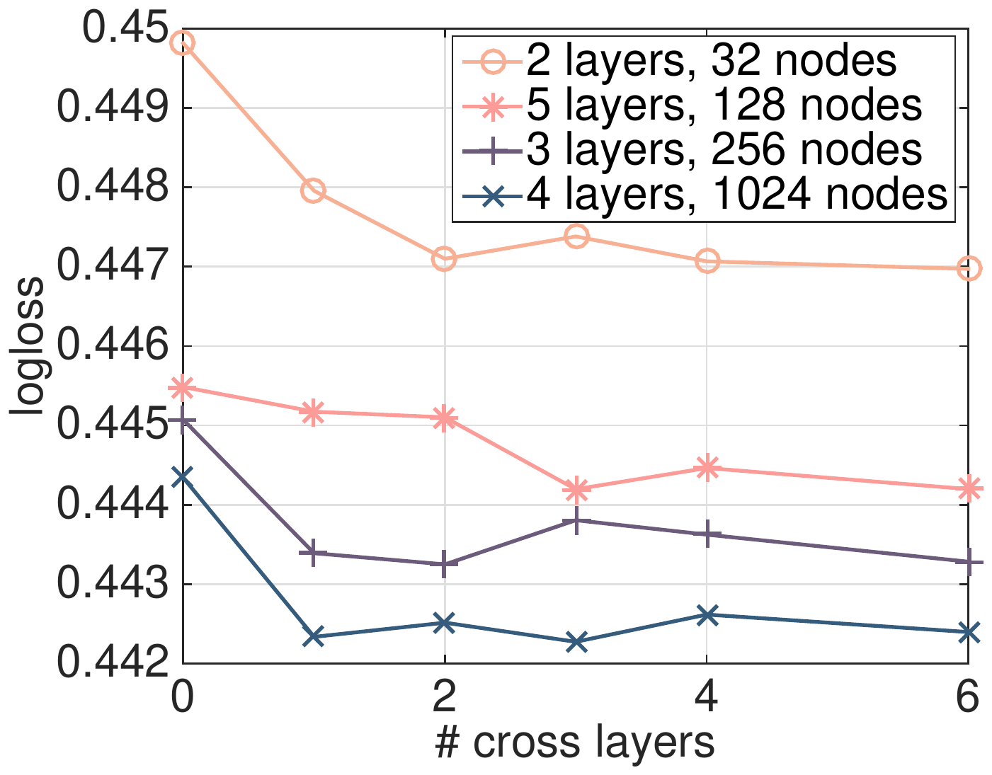
Figure 3 shows the improvement as we increase the number of cross layers on randomly selected settings. For the deep networks in Figure 3, there is a clear improvement when 1 cross layer is added to the model. As more cross layers are introduced, for some settings the logloss continues to decrease, indicating the introduced cross terms are effective in the prediction; whereas for others the logloss starts to fluctuate and even slightly increase, which indicates the higher-degree feature interactions introduced are not helpful.

4.5 Non-CTR datasets

We show that DCN performs well on non-CTR prediction problems. We used the forest covertype (581012 samples and 54 features) and Higgs (11M samples and 28 features) datasets from the UCI repository. The datasets were randomly split into training (90%) and testing (10%) set. A grid search over the hyperparameters was performed. The number of deep layers ranged from 1 to 10 with layer size from 50 to 300. The number of cross layers ranged from 4 to 10. The number of residual units ranged from 1 to 5 with their input dimension and cross dimension from 50 to 300. For DCN, the input vector was fed to the cross network directly.

For the forest covertype data, DCN achieved the best test accuracy 0.9740 with the least memory consumption. Both DNN and DC achieved 0.9737. The optimal hyperparameter settings were 8 cross layers of size 54 and 6 deep layers of size 292 for DCN, 7 deep layers of size 292 for DNN, and 4 residual units with input dimension 271 and cross dimension 287 for DC.

For the Higgs data, DCN achieved the best test logloss 0.4494, whereas DNN achieved 0.4506. The optimal hyperparameter settings were 4 cross layers of size 28 and 4 deep layers of size 209 for DCN, and 10 deep layers of size 196 for DNN. DCN outperforms DNN with half of the memory used in DNN.

5. Conclusion and Future Directions

Section Summary: The conclusion notes that manually designing feature interactions is tedious and that standard deep networks, while automatic, tend to produce implicit and inefficient representations. The proposed Deep & Cross Network overcomes these limits by jointly learning explicit, bounded-degree cross features together with conventional deep representations, delivering higher accuracy and lower memory use on both sparse and dense data. Future work will examine cross layers as modular components in other models, methods for training deeper cross networks, and the mathematical and optimization behavior of the architecture.

Identifying effective feature interactions has been the key to the success of many prediction models. Regrettably, the process often requires manual feature crafting and exhaustive searching. DNNs are popular for automatic feature learning; however, the features learned are implicit and highly nonlinear, and the network could be unnecessarily large and inefficient in learning certain features. The Deep & Cross Network proposed in this paper can handle a large set of sparse and dense features, and learns explicit cross features of bounded degree jointly with traditional deep representations. The degree of cross features increases by one at each cross layer. Our experimental results have demonstrated its superiority over the state-of-art algorithms on both sparse and dense datasets, in terms of both model accuracy and memory usage.

We would like to further explore using cross layers as building blocks in other models, enable effective training for deeper cross networks, investigate the efficiency of the cross network in polynomial approximation, and better understand its interaction with deep networks during optimization.

Appendix: Proof of Theorem 3.1

Proof: Notations. Let ${\bf i}$ be a multi-index vector of 0's and 1's with its last entry fixed at 1. For multi-index ${\bm \alpha} = [\alpha_1, \cdot s, \alpha_d] \in \mathbb{N}^d$ and ${\bf x} = [x_1, \cdot s, x_d]^T$, we define $| {\bm \alpha}| = \sum_{i=1}^d \alpha_i$, and ${\bf x}^{{\bm \alpha}} = x_1^{\alpha_1}x_2^{\alpha_2}\cdot s x_d^{\alpha_d}$.

We first proof by induction that

$ g_l({\bf x}0) = {\bf x}l^T {\bf w}l = \sum{p=1}^{l+1} \sum{\substack{| {\bf i}| = p }} \prod{j=0}^{l} ({\bf x}_0^T {\bf w}_j)^{i_j},\tag{3} $

and then we rewrite the above form to obtain the desired claim.

• Base case. When $l = 0$, $g_0({\bf x}_0) = {\bf x}_0^T {\bf w}_0$. Clearly Equation 3 holds.
• Induction step. We assume that when $l = k$,

$ g_k({\bf x}0) = {\bf x}k^T {\bf w}k = \sum{p=1}^{k+1} \sum{\substack{| {\bf i}| = p}} \prod{j=0}^{k} ({\bf x}_0^T {\bf w}_j)^{i_j}. $

When $l = k+1$,

$ \begin{split} {\bf x}{k+1}^T {\bf w}{k+1} = ({\bf x}_k^T {\bf w}_k) ({\bf x}0^T {\bf w}{k+1}) + {\bf x}k^T {\bf w}{k+1} \end{split} $

Because ${\bf x}k$ only contains ${\bf w}0, \ldots, {\bf w}{k-1}$, it follows that the formula of ${\bf x}{k}^T {\bf w}{k+1}$ can be obtained from that of ${\bf x}{k}^T {\bf w}{k}$ by replacing all the ${\bf w}k$ 's occurred in ${\bf x}{k}^T {\bf w}{k}$ to ${\bf w}_{k+1}$. Then

$ \begin{split}& {\bf x}{k+1}^T {\bf w}{k+1} =\& \sum_{p=1}^{k+1} \sum_{\substack{| {\bf i}| = p}}({\bf x}0^T {\bf w}{k+1}) \prod_{j=0}^{k} ({\bf x}0^T {\bf w}j)^{i_j} + \sum{p=1}^{k+1} \sum{\substack{| {\bf i}| = p }} ({\bf x}0^T {\bf w}{k+1})^{i_k}\prod_{j=0}^{k-1} ({\bf x}0^T {\bf w}j)^{i_j}\= & \sum{p=2}^{k+2} \sum{\substack{| {\bf i}| = p\ i_k = 1}} \prod_{j=0}^{k+1} ({\bf x}0^T {\bf w}j)^{i_j} + \sum{p=1}^{k+1} \sum{\substack{| {\bf i}| = p\ i_{k} = 0}} \prod_{j=0}^{k+1} ({\bf x}0^T {\bf w}j)^{i_j}\= &\sum{p=2}^{k+1} \sum{\substack{| {\bf i}| = p}} \prod_{j=0}^{k+1} ({\bf x}0^T {\bf w}j)^{i_j} + ({\bf x}0^T {\bf w}{k+1}) + \prod{j=0}^{k+1} ({\bf x}0^T {\bf w}j)\= & \sum{p=1}^{k+2} \sum{\substack{| {\bf i}| = p}} \prod{j=0}^{k+1} ({\bf x}_0^T {\bf w}_j)^{i_j}.\end{split} $

The first equality is a result of increasing the size of ${\bf i}$ from $k+1$ to $k+2$.

The second equality used the fact that the last entry of ${\bf i}$ is always 1 by definition, and the same was applied to the last equality.

By induction hypothesis, Equation 3 holds for all $l \in \mathbb{Z}$.

Next, we compute $c_{\bm \alpha}({\bf w}0, \cdot s, {\bf w}l)$, the coefficient of ${\bf x}^{\bm \alpha}$, by rearranging the terms in Equation 3. Note that all the different permutations of $\underbrace{x_1 \cdot s x_1}{\alpha_1} \cdot s \underbrace{x_d \cdot s x_d}{\alpha_d}$ are in the form of ${\bf x}^{\bm \alpha}$. Therefore, $c_{\bm \alpha}$ is the summation of all the weights associated with each permutation occurred in Equation 3. The weight for permutation $x_{j_1} x_{j_2} \cdot s x_{j_p}$ is

$ \sum_{i_1, \cdot s, i_p} w_{i_1}^{(j_1)} w_{i_2}^{(j_2)} \cdot s w_{i_p}^{(j_p)}, $

where $(i_1, \cdot s, i_p)$ belongs to the set of all the corresponding active indices for $| {\bf i}|=p$, specifically,

$ (i_1, \cdot s, i_p) \in B_p =: \bigl{{\bf y} \in {0, 1, \cdot s, l}^{p} \mathrel{\big|} y_i < y_j \wedge y_{p} = l\bigr}. $

Therefore, if we denote $P_{\bm \alpha}$ to be the set of all the permutations of $(\underbrace{1 \cdot s 1}{\alpha_1} \cdot s \underbrace{d \cdot s d}{\alpha_d})$, then we arrive at our claim

$ c_{\bm \alpha} = \sum_{j_1, \cdot s, j_p \in P_p} \sum_{i_1, \cdot s, i_p \in B_p} \prod_{k=1}^p w_{i_k}^{(j_k)}. $

References

Section Summary: The references list foundational and recent research papers primarily on machine learning techniques for large-scale recommendation and advertising systems. They cover core topics such as deep learning architectures, factorization machines and their extensions for predicting user clicks, and hybrid models that combine wide linear and deep neural components. Additional citations address practical tools for training these systems, including optimization methods and normalization strategies used in real-world deployments.

[1] Olivier Chapelle, Eren Manavoglu, and Romer Rosales.2015. Simple and scalable response prediction for display advertising. *ACM Transactions on Intelligent Systems and Technology (TIST)*5, 4(2015), 61.

[2] Yann LeCun, Yoshua Bengio, and Geoffrey Hinton.2015. Deep learning. Nature521, 7553(2015), 436–444.

[3] Jürgen Schmidhuber.2015. Deep learning in neural networks: An overview. Neural networks61(2015), 85–117.

[4] Steffen Rendle.2010. Factorization machines. In 2010 IEEE International Conference on Data Mining. IEEE, 995–1000.

[5] Steffen Rendle.2012. Factorization Machines with libFM. *ACM Trans. Intell. Syst. Technol.*3, 3, Article 57(May2012), 22 pages.

[6] Yuchin Juan, Yong Zhuang, Wei-Sheng Chin, and Chih-Jen Lin.2016. Field-aware factorization machines for CTR prediction. In Proceedings of the 10th ACM Conference on Recommender Systems. ACM, 43–50.

[7] Yuchin Juan, Damien Lefortier, and Olivier Chapelle.2017. Field-aware factorization machines in a real-world online advertising system. In Proceedings of the 26th International Conference on World Wide Web Companion. International World Wide Web Conferences Steering Committee, 680–688.

[8] Mathieu Blondel, Akinori Fujino, Naonori Ueda, and Masakazu Ishihata.2016. Higher-Order Factorization Machines. In Advances in Neural Information Processing Systems. 3351–3359.

[9] Jiyan Yangand Alex Gittens.2015. Tensor machines for learning target-specific polynomial features. arXiv preprint arXiv:1504.01697(2015).

[10] Kaiming He, Xiangyu Zhang, Shaoqing Ren, and Jian Sun.2015. Deep residual learning for image recognition. arXiv preprint arXiv:1512.03385(2015).

[11] Ying Shan, T Ryan Hoens, Jian Jiao, Haijing Wang, Dong Yu, and JC Mao.2016. Deep Crossing: Web-Scale Modeling without Manually Crafted Combinatorial Features. In Proceedings of the 22nd ACM SIGKDD International Conference on Knowledge Discovery and Data Mining. ACM, 255–262.

[12] Gregory Valiant.2014. Learning polynomials with neural networks. (2014).

[13] Andreas Veit, Michael J Wilber, and Serge Belongie.2016. Residual Networks Behave Like Ensembles of Relatively Shallow Networks. In Advances in Neural Information Processing Systems 29, D. D. Lee, M. Sugiyama, U. V. Luxburg, I. Guyon, and R. Garnett(Eds.). Curran Associates, Inc., 550–558.

[14] Heng-Tze Cheng, Levent Koc, Jeremiah Harmsen, Tal Shaked, Tushar Chandra, Hrishi Aradhye, Glen Anderson, Greg Corrado, Wei Chai, Mustafa Ispir, and others.2016. Wide & Deep Learning for Recommender Systems. arXiv preprint arXiv:1606.07792(2016).

[15] Walter Rudinand others.1964. Principles of mathematical analysis. Vol. 3. McGraw-Hill New York.

[16] Diederik Kingmaand Jimmy Ba.2014. Adam: A method for stochastic optimization. arXiv preprint arXiv:1412.6980(2014).

[17] Sergey Ioffeand Christian Szegedy.2015. Batch normalization: Accelerating deep network training by reducing internal covariate shift. arXiv preprint arXiv:1502.03167(2015).

[18] K. Canini.2012. Sibyl: A system for large scale supervised machine learning.Technical Talk(2012).