Variational Diffusion Models

Diederik P. Kingma$^{}$, Tim Salimans$^{}$, Ben Poole, Jonathan Ho
Google Research

* Equal contribution.35th Conference on Neural Information Processing Systems (NeurIPS 2021).

Abstract

Section Summary: Diffusion-based generative models, which create realistic images by gradually adding and removing noise, have long excelled at visual synthesis but were questioned for their ability to accurately estimate data probabilities. This work introduces a new type of these models that achieves top performance on standard image probability benchmarks, with innovations like efficiently tuning the noise process alongside the model and simplifying key math to a brief formula based on signal-to-noise ratios. These advances also reveal connections between existing models, enable faster training by minimizing estimation errors, and outperform traditional autoregressive methods, while supporting near-optimal image compression techniques.

Diffusion-based generative models have demonstrated a capacity for perceptually impressive synthesis, but can they also be great likelihood-based models? We answer this in the affirmative, and introduce a family of diffusion-based generative models that obtain state-of-the-art likelihoods on standard image density estimation benchmarks. Unlike other diffusion-based models, our method allows for efficient optimization of the noise schedule jointly with the rest of the model. We show that the variational lower bound (VLB) simplifies to a remarkably short expression in terms of the signal-to-noise ratio of the diffused data, thereby improving our theoretical understanding of this model class. Using this insight, we prove an equivalence between several models proposed in the literature. In addition, we show that the continuous-time VLB is invariant to the noise schedule, except for the signal-to-noise ratio at its endpoints. This enables us to learn a noise schedule that minimizes the variance of the resulting VLB estimator, leading to faster optimization. Combining these advances with architectural improvements, we obtain state-of-the-art likelihoods on image density estimation benchmarks, outperforming autoregressive models that have dominated these benchmarks for many years, with often significantly faster optimization. In addition, we show how to use the model as part of a bits-back compression scheme, and demonstrate lossless compression rates close to the theoretical optimum. Code is available at https://github.com/google-research/vdm.

Executive Summary: Generative models in machine learning aim to capture the underlying distribution of data, such as images, to enable tasks like synthesis, compression, and anomaly detection. For years, autoregressive models have led in accurately estimating data likelihoods on benchmarks like CIFAR-10 and ImageNet, measuring how well a model assigns probabilities to real images. Diffusion models, which progressively add and remove noise to generate data, have excelled in producing visually striking samples but trailed in likelihood accuracy. With growing demands for efficient, high-fidelity generative tools in fields like computer vision and data compression, improving diffusion models' density estimation capabilities is timely to challenge autoregressive dominance and expand their practical use.

This paper introduces variational diffusion models (VDMs), a new class designed to maximize likelihoods while retaining diffusion's strengths in sample quality. The goal was to develop and test these models on standard image benchmarks, demonstrating superior performance over prior approaches, including autoregressive baselines.

The authors built VDMs by treating diffusion processes as variational autoencoders, where data is gradually noised forward and denoised backward through a hierarchy of latent variables. They derived a simplified objective function based on signal-to-noise ratios, proved theoretical equivalences between diffusion variants, and optimized noise schedules jointly with model parameters using neural networks. Key innovations included Fourier features to better capture pixel-level details and continuous-time formulations for deeper hierarchies. Experiments used CIFAR-10 (50,000 training images of 32x32 pixels) and downsampled ImageNet (1.2 million 32x32 or 64x64 images), with training on GPU/TPU hardware over days to weeks; assumptions included Gaussian noise and variance-preserving diffusion, evaluated via variational bounds without full likelihood computation.

The core results show VDMs achieving state-of-the-art likelihoods: 2.65 bits per dimension (BPD, a lower value indicates better density estimation) on unaugmented CIFAR-10, improving to 2.49 with augmentations—about 10% better than the prior best autoregressive model and 5-10% ahead of concurrent diffusion works. On ImageNet, scores reached 3.72 BPD for 32x32 and 3.40 for 64x64, surpassing previous leaders by 4-8%. Continuous-time versions optimized 10 times faster than top autoregressive models on equivalent hardware. Additional tests confirmed near-optimal lossless compression rates on CIFAR-10, with net lengths 0.03-0.07 BPD above the theoretical minimum for moderate depths. Samples retained strong perceptual quality, with Fréchet Inception Distance scores of 4.0-7.4, competitive but not optimized for visuals.

These findings mean diffusion models can now rival or exceed autoregressive ones in precise probability modeling, unlocking benefits like faster training (hours vs. days) and scalability to complex data. This shifts risks in generative tasks toward more reliable likelihoods, reducing errors in applications like image compression (saving 5-10% more bits) or anomaly detection (better identifying outliers). Unlike expectations that diffusion would lag in exactness due to its noise-based nature, VDMs close the gap through theoretical insights, proving many prior models equivalent and invariant to schedule shapes—simplifying design and explaining past inconsistencies.

Leaders should prioritize VDMs for new density estimation projects, integrating them into pipelines for image synthesis or compression to gain efficiency gains. For compression, deploy discrete-time versions with bits-back coding at 250-1000 steps, balancing cost and performance; trade-offs include higher compute for deeper models yielding 1-2% better rates. Next steps involve piloting on higher-resolution datasets (e.g., 128x128+), refining bits-back for very deep hierarchies to close the 0.05 BPD gap, and testing weighted objectives for hybrid likelihood-perceptual goals. Further analysis could explore conditional variants for tasks like editing.

While robust across hardware and validated on established benchmarks, limitations include reliance on variational bounds (potentially underestimating true likelihood by 0.05-0.10 BPD) and focus on images, with untested generalization to video or text. Assumptions like fixed endpoints in noise schedules hold under experiments but may falter in diverse domains. Confidence is high in benchmark superiority, supported by ablations showing Fourier features and learned schedules driving 20-30% gains, though readers should verify on custom data before broad decisions.

1 Introduction

Section Summary: Likelihood-based generative modeling is a key area in machine learning that powers applications like speech synthesis, translation, and data compression. For years, autoregressive models have led the way because they efficiently estimate data probabilities and capture complex patterns, outperforming newer diffusion models—which excel at creating high-quality images and audio but fall short on standard density estimation tests. This paper introduces Variational Diffusion Models, a new type of diffusion model enhanced with techniques like Fourier features and customizable noise processes, which now achieve top results on image benchmarks and come with fresh theoretical insights into how these models work under the hood.

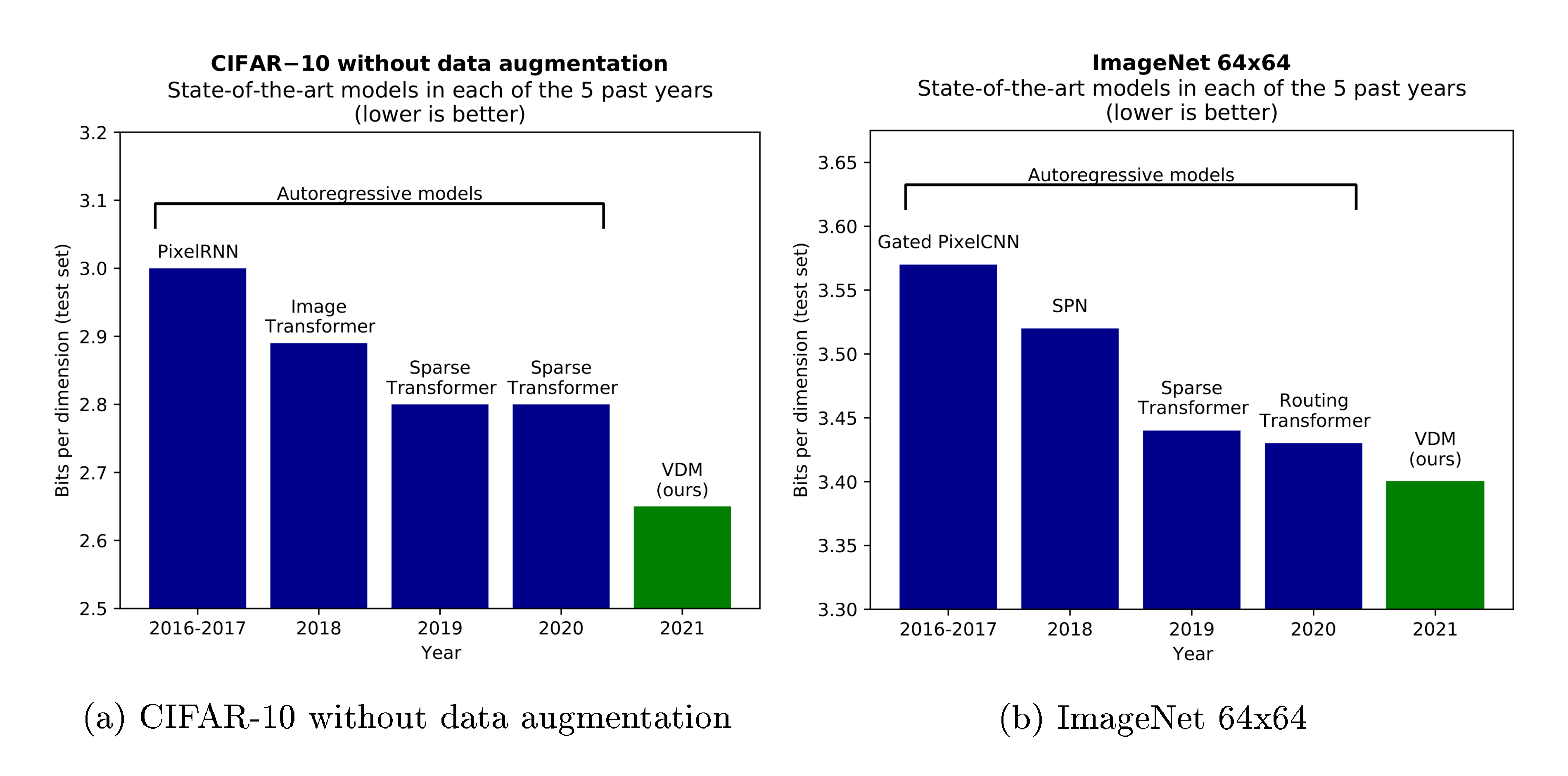
Likelihood-based generative modeling is a central task in machine learning that is the basis for a wide range of applications ranging from speech synthesis [1], to translation [2], to compression [3], to many others. Autoregressive models have long been the dominant model class on this task due to their tractable likelihood and expressivity, as shown in Figure 1. Diffusion models have recently shown impressive results in image [4, 5, 6] and audio generation [7, 8] in terms of perceptual quality, but have yet to match autoregressive models on density estimation benchmarks. In this paper we make several technical contributions that allow diffusion models to challenge the dominance of autoregressive models in this domain.

Our main contributions are as follows:

• We introduce a flexible family of diffusion-based generative models that achieve new state-of-the-art log-likelihoods on standard image density estimation benchmarks (CIFAR-10 and ImageNet). This is enabled by incorporating Fourier features into the diffusion model and using a learnable specification of the diffusion process, among other modeling innovations.
• We improve our theoretical understanding of density modeling using diffusion models by analyzing their variational lower bound (VLB), deriving a remarkably simple expression in terms of the signal-to-noise ratio of the diffusion process. This result delivers new insight into the model class: for the continuous-time (infinite-depth) setting we prove a novel invariance of the generative model and its VLB to the specification of the diffusion process, and we show that various diffusion models from the literature are equivalent up to a trivial time-dependent rescaling of the data.

2 Related work

Section Summary: This section discusses how the authors' research draws from diffusion probabilistic models, a type of generative AI similar to variational autoencoders, which have gained popularity for creating high-quality images. It reviews key advancements, such as improvements in training techniques by Ho and others for better image generation, score matching methods by Song and Ermon for efficient learning, and extensions to continuous-time processes with variational bounds in recent works by Song, Huang, Vahdat, and colleagues. Unlike prior approaches that fixed the diffusion process, the authors optimize it alongside the model, use direct parameterization of data distributions, and incorporate Fourier features to achieve superior performance, with empirical comparisons showing their advantages.

Our work builds on diffusion probabilistic models (DPMs) [9], or diffusion models in short. DPMs can be viewed as a type of variational autoencoder (VAE) [10, 11], whose structure and loss function allows for efficient training of arbitrarily deep models. Interest in diffusion models has recently reignited due to their impressive image generation results [4, 12].

Ho et al. [4] introduced a number of model innovations to the original DPM, with impressive results on image generation quality benchmarks. They showed that the VLB objective, for a diffusion model with discrete time and diffusion variances shared across input dimensions, is equivalent to multi-scale denoising score matching, up to particular weightings per noise scale. Further improvements were proposed by Nichol and Dhariwal [6], resulting in better log-likelihood scores. Gao et al. [13] show how diffusion can also be used to efficiently optimize energy-based models (EBMs) towards a close approximation of the log-likelihood objective, resulting in high-fidelity samples even after long MCMC chains.

Song and Ermon [14] first proposed learning generative models through a multi-scale denoising score matching objective, with improved methods in Song and Ermon [12]. This was later extended to continuous-time diffusion with novel sampling algorithms based on reversing the diffusion process [5].

Concurrent to our work, Song et al. [15], Huang et al. [16], and Vahdat et al. [17] also derived variational lower bounds to the data likelihood under a continuous-time diffusion model. Where we consider the infinitely deep limit of a standard VAE, Song et al. [15] and Vahdat et al. [17] present different derivations based on stochastic differential equations. Huang et al. [16] considers both perspectives and discusses the similarities between the two approaches. An advantage of our analysis compared to these other works is that we present an intuitive expression of the VLB in terms of the signal-to-noise ratio of the diffused data, leading to much simplified expressions of the discrete-time and continuous-time loss, allowing for simple and numerically stable implementation. This also leads to new results on the invariance of the generative model and its VLB to the specification of the diffusion process. We empirically compare to these works, as well as others, in Table 1.

Previous approaches to diffusion probabilistic models fixed the diffusion process; in contrast optimize the diffusion process parameters jointly with the rest of the model. This turns the model into a type of VAE ([10, 11]). This is enabled by directly parameterizing the mean and variance of the marginal $q({\mathbf{z}}_t| {\mathbf{z}}0)$, where previous approaches instead parameterized the individual diffusion steps $q({\mathbf{z}}{t+\epsilon}| {\mathbf{z}}_t)$. In addition, our denoising models include several architecture changes, the most important of which is the use of Fourier features, which enable us to reach much better likelihoods than previous diffusion probabilistic models.

3 Model

Section Summary: This section describes a basic generative model for estimating the distribution of data, like images, by using a diffusion process that starts with the original data and gradually adds noise over time to create a series of increasingly blurry latent versions, from clear at the start to pure noise at the end. The noise level is controlled by a learnable schedule, ensuring the process gets steadily messier, and this forward diffusion follows Gaussian patterns with a decreasing signal-to-noise ratio. To generate new data, the model reverses this by starting from noise and step by step removing it to reconstruct clear samples, forming a hierarchical structure that's optimized using a simple bound on the data likelihood.

We will focus on the most basic case of generative modeling, where we have a dataset of observations of ${\mathbf{x}}$, and the task is to estimate the marginal distribution $p({\mathbf{x}})$. As with most generative models, the described methods can be extended to the case of multiple observed variables, and/or the task of estimating conditional densities $p({\mathbf{x}}| {\mathbf{y}})$. The proposed latent-variable model consists of a diffusion process (Section 3.1) that we invert to obtain a hierarchical generative model (Section 3.3). As we will show, the model choices below result in a surprisingly simple variational lower bound (VLB) of the marginal likelihood, which we use for optimization of the parameters.

3.1 Forward time diffusion process

Our starting point is a Gaussian diffusion process that begins with the data ${\mathbf{x}}$, and defines a sequence of increasingly noisy versions of ${\mathbf{x}}$ which we call the latent variables ${\mathbf{z}}_t$, where $t$ runs from $t=0$ (least noisy) to $t=1$ (most noisy). The distribution of latent variable ${\mathbf{z}}_t$ conditioned on ${\mathbf{x}}$, for any $t \in [0, 1]$ is given by:

$ \begin{align} q({\mathbf{z}}_t| {\mathbf{x}}) &= \mathcal{N}\left(\alpha_t {\mathbf{x}}, \sigma^2_t \mathbf{I}\right), \end{align}\tag{1} $

where $\alpha_t$ and $\sigma^{2}_t$ are strictly positive scalar-valued functions of $t$. Furthermore, let us define the signal-to-noise ratio (SNR):

$ \begin{align} \text{SNR}(t) = \alpha^2_t / \sigma^2_t. \end{align} $

We assume that the $\text{SNR}(t)$ is strictly monotonically decreasing in time, i.e. that $\text{SNR}(t) < \text{SNR}(s)$ for any $t > s$. This formalizes the notion that the ${\mathbf{z}}t$ is increasingly noisy as we go forward in time. We also assume that both $\alpha{t}$ and $\sigma^{2}_t$ are smooth, such that their derivatives with respect to time $t$ are finite. This diffusion process specification includes the variance-preserving diffusion process as used by [9, 4] as a special case, where $\alpha_t = \sqrt{1 - \sigma^2_t}$. Another special case is the variance-exploding diffusion process as used by [14, 5], where $\alpha^2_t = 1$. In experiments, we use the variance-preserving version.

The distributions $q({\mathbf{z}}_t| {\mathbf{z}}_s)$ for any $t > s$ are also Gaussian, and given in Appendix A. The joint distribution of latent variables $({\mathbf{z}}_s, {\mathbf{z}}_t, {\mathbf{z}}_u)$ at any subsequent timesteps $0 \leq s < t < u \leq 1$ is Markov: $q({\mathbf{z}}_u | {\mathbf{z}}_t, {\mathbf{z}}_s) = q({\mathbf{z}}_u | {\mathbf{z}}_t)$. Given the distributions above, it is relatively straightforward to verify through Bayes rule that $q({\mathbf{z}}_s| {\mathbf{z}}_t, {\mathbf{x}})$, for any $0 \leq s < t \leq 1$, is also Gaussian. This distribution is also given in Appendix A.

3.2 Noise schedule

In previous work, the noise schedule has a fixed form (see Appendix H, Figure 4a). In contrast, we learn this schedule through the parameterization

$ \begin{align} \sigma^{2}t = \text{sigmoid}(\gamma{{\boldsymbol{\eta}}}(t)) \end{align} $

where $\gamma_{{\boldsymbol{\eta}}}(t)$ is a monotonic neural network with parameters ${{\boldsymbol{\eta}}}$, as detailed in Appendix H.

Motivated by the equivalence discussed in Section 5.1, we use $\alpha_t = \sqrt{1 - \sigma^2_t}$ in our experiments for both the discrete-time and continuous-time models, i.e. variance-preserving diffusion processes. It is straightforward to verify that $\alpha^2_t$ and $\text{SNR}(t)$, as a function of $\gamma_{{\boldsymbol{\eta}}}(t)$, then simplify to:

$ \begin{align} \alpha^{2}t = \text{sigmoid}(-\gamma{{\boldsymbol{\eta}}}(t)) \ \text{SNR}(t) = \exp(-\gamma_{{\boldsymbol{\eta}}}(t)) \end{align} $

3.3 Reverse time generative model

We define our generative model by inverting the diffusion process of Section 3.1, yielding a hierarchical generative model that samples a sequence of latents ${\mathbf{z}}_t$, with time running backward from $t=1$ to $t=0$. We consider both the case where this sequence consists of a finite number of steps $T$, as well as a continuous time model corresponding to $T\rightarrow\infty$. We start by presenting the discrete-time case.

Given finite $T$, we discretize time uniformly into $T$ timesteps (segments) of width $\tau = 1/T$. Defining $s(i) = (i-1)/T$ and $t(i) = i/T$, our hierarchical generative model for data ${\mathbf{x}}$ is then given by:

$ \begin{align} p({\mathbf{x}}) &= \int_{{\mathbf{z}}} p({\mathbf{z}}{1})p({\mathbf{x}}| {\mathbf{z}}{0}) \prod_{i=1}^T p({\mathbf{z}}{s(i)}| {\mathbf{z}}{t(i)}). \end{align} $

With the variance preserving diffusion specification and sufficiently small $\text{SNR}(1)$, we have that $q({\mathbf{z}}_1| {\mathbf{x}}) \approx \mathcal{N}({\mathbf{z}}_1; 0, \mathbf{I})$. We therefore model the marginal distribution of ${\mathbf{z}}_1$ as a spherical Gaussian:

$ \begin{align} p({\mathbf{z}}_1) = \mathcal{N}({\mathbf{z}}_1; 0, \mathbf{I}). \end{align} $

We wish to choose a model $p({\mathbf{x}}| {\mathbf{z}}_0)$ that is close to the unknown $q({\mathbf{x}}| {\mathbf{z}}0)$. Let $x_i$ and $z{0, i}$ be the $i$-th elements of ${\mathbf{x}}, {\mathbf{z}}_0$, respectively. We then use a factorized distribution of the form:

$ \begin{align} p({\mathbf{x}}| {\mathbf{z}}0) = \prod_i p(x_i|z{0, i}), \end{align}\tag{2} $

where we choose $p(x_i |z_{0, i}) \propto q(z_{0, i}|x_i)$, which is normalized by summing over all possible discrete values of $x_i$ (256 in the case of 8-bit image data). With sufficiently large $\text{SNR}(0)$, this becomes a very close approximation to the true $q({\mathbf{x}}| {\mathbf{z}}_0)$, as the influence of the unknown data distribution $q({\mathbf{x}})$ is overwhelmed by the likelihood $q({\mathbf{z}}_0| {\mathbf{x}})$. Finally, we choose the conditional model distributions as

$ \begin{align} p({\mathbf{z}}_s| {\mathbf{z}}_t) = q({\mathbf{z}}_s| {\mathbf{z}}t, {\mathbf{x}}=\hat{{\mathbf{x}}}{{\boldsymbol{\theta}}}({\mathbf{z}}_t; t)), \end{align} $

i.e. the same as $q({\mathbf{z}}_s| {\mathbf{z}}t, \mathbf{x})$, but with the original data ${\mathbf{x}}$ replaced by the output of a denoising model $\hat{{\mathbf{x}}}{{\boldsymbol{\theta}}}({\mathbf{z}}_t; t)$ that predicts ${\mathbf{x}}$ from its noisy version ${\mathbf{z}}_t$. Note that in practice we parameterize the denoising model as a function of a noise prediction model (Section 3.4), bridging the gap with previous work on diffusion models [4]. The means and variances of $p({\mathbf{z}}_s| {\mathbf{z}}_t)$ simplify to a remarkable degree; see Appendix A.

3.4 Noise prediction model and Fourier features

We parameterize the denoising model in terms of a noise prediction model $\hat{{\boldsymbol{\epsilon}}}_{{\boldsymbol{\theta}}}({\mathbf{z}}_t; t)$:

$ \begin{align} \hat{{\mathbf{x}}}_{{\boldsymbol{\theta}}}({\mathbf{z}}_t; t) = ({\mathbf{z}}t - \sigma_t \hat{{\boldsymbol{\epsilon}}}{{\boldsymbol{\theta}}}({\mathbf{z}}_t; t))/\alpha_t, \end{align}\tag{3} $

where $\hat{{\boldsymbol{\epsilon}}}_{{\boldsymbol{\theta}}}({\mathbf{z}}_t; t)$ is parameterized as a neural network. The noise prediction models we use in experiments closely follow [4], except that they process the data solely at the original resolution. The exact parameterization of the noise prediction model and noise schedule is discussed in Appendix B.

Prior work on diffusion models has mainly focused on the perceptual quality of generated samples, which emphasizes coarse scale patterns and global consistency of generated images. Here, we optimize for likelihood, which is sensitive to fine scale details and exact values of individual pixels. To capture the fine scale details of the data, we propose adding a set of Fourier features to the input of our noise prediction model. Let ${\mathbf{x}}$ be the original data, scaled to the range $[-1, 1]$, and let ${\mathbf{z}}$ be the resulting latent variable, with similar magnitudes. We then append channels $\sin(2^n\pi {\mathbf{z}})$ and $\cos(2^n\pi {\mathbf{z}})$, where $n$ runs over a range of integers ${n_{min}, ..., n_{max}}$. These features are high frequency periodic functions that amplify small changes in the input data ${\mathbf{z}}_t$; see Appendix C for further details. Including these features in the input of our denoising model leads to large improvements in likelihood as demonstrated in Section 6 and Figure 5, especially when combined with a learnable SNR function. We did not observe such improvements when incorporating Fourier features into autoregressive models.

3.5 Variational lower bound

We optimize the parameters towards the variational lower bound (VLB) of the marginal likelihood, which is given by

$ \begin{align}

• \log p({\mathbf{x}}) \leq
  • \text{VLB}({\mathbf{x}}) = \underbrace{ D_{KL}(q({\mathbf{z}}_1| {\mathbf{x}})||p({\mathbf{z}}1)) }{\text{Prior loss}}
  • \underbrace{ \mathbb{E}_{q({\mathbf{z}}_0| {\mathbf{x}})}\left[- \log p({\mathbf{x}}| {\mathbf{z}}0) \right] }{\text{Reconstruction loss}}
  • \underbrace{ \mathcal{L}T({\mathbf{x}}). }{\text{Diffusion loss}} \end{align}\tag{4} $

The prior loss and reconstruction loss can be (stochastically and differentiably) estimated using standard techniques; see ([10]). The diffusion loss, $\mathcal{L}_T({\mathbf{x}})$, is more complicated, and depends on the hyperparameter $T$ that determines the depth of the generative model.

4 Discrete-time model

Section Summary: This section describes a discrete-time version of the diffusion model, where the process is broken into a finite number of steps T, leading to a simplified loss function that measures how well the model predicts noise or images at different points along the way. By using specific noise schedules, the loss becomes a straightforward average of errors weighted by changes in signal-to-noise ratios, which can be efficiently optimized with random sampling and is stable even on basic computer hardware. It also explains that using more steps T generally reduces the overall loss, as it provides a closer approximation to the ideal continuous process, much like refining a rough sketch into a detailed drawing.

In the case of finite $T$, using $s(i) = (i-1)/T$, $t(i) = i/T$, the diffusion loss is:

$ \begin{align} \mathcal{L}T({\mathbf{x}}) &= \sum{i=1}^T \mathbb{E}{q({\mathbf{z}}{t(i)}| {\mathbf{x}})} D_{KL}[q({\mathbf{z}}{s(i)}| {\mathbf{z}}{t(i)}, {\mathbf{x}})||p({\mathbf{z}}{s(i)}| {\mathbf{z}}{t(i)})]. \end{align}\tag{5} $

In Appendix E we show that this expression simplifies considerably, yielding:

$ \begin{align} \mathcal{L}T({\mathbf{x}}) = \frac{T}{2} \mathbb{E}{{\boldsymbol{\epsilon}} \sim \mathcal{N}(0, \mathbf{I}), i \sim U{1, T}} \left[\left(\text{SNR}(s)-\text{SNR}(t)\right) || {\mathbf{x}} - \hat{{\mathbf{x}}}_{{\boldsymbol{\theta}}}({\mathbf{z}}_t;t) ||_2^2 \right], \end{align}\tag{6} $

where $U{1, T}$ is the uniform distribution on the integers ${1, \ldots, T}$, and ${\mathbf{z}}t = \alpha_t {\mathbf{x}} + \sigma_t {\boldsymbol{\epsilon}}$. This is the general discrete-time loss for any choice of forward diffusion parameters $(\sigma_t, \alpha_t)$. When plugging in the specifications of $\sigma_t$, $\alpha_t$ and $\hat{{\mathbf{x}}}{{\boldsymbol{\theta}}}({\mathbf{z}}_t; t)$ that we use in experiments, given in Section 3.2 and Section 3.4, the loss simplifies to:

$ \begin{align} \mathcal{L}T({\mathbf{x}}) = \frac{T}{2} \mathbb{E}{{\boldsymbol{\epsilon}} \sim \mathcal{N}(0, \mathbf{I}), i \sim U{1, T}} \left[(\exp(\gamma_{{\boldsymbol{\eta}}}(t)-\gamma_{{\boldsymbol{\eta}}}(s))-1) \left\lVert {\boldsymbol{\epsilon}} - \hat{{\boldsymbol{\epsilon}}}_{{\boldsymbol{\theta}}}({\mathbf{z}}_t; t) \right\lVert_2^2 \right] \end{align}\tag{7} $

where ${\mathbf{z}}t = \text{sigmoid}(-\gamma{{\boldsymbol{\eta}}}(t)) {\mathbf{x}} + \text{sigmoid}(\gamma_{{\boldsymbol{\eta}}}(t)) {\boldsymbol{\epsilon}}$. In the discrete-time case, we simply jointly optimize ${\boldsymbol{\eta}}$ and ${\boldsymbol{\theta}}$ by maximizing the VLB through a Monte Carlo estimator of Equation 7.

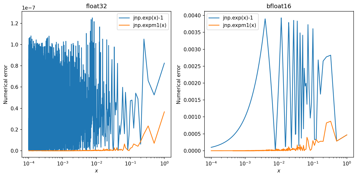
Note that $\exp(.)-1$ has a numerically stable primitive $expm1(.)$ in common numerical computing packages; see Figure 6. Equation 7 allows for numerically stable implementation in 32-bit or lower-precision floating point, in contrast with previous implementations of discrete-time diffusion models (e.g. ([4])), which had to resort to 64-bit floating point.

4.1 More steps leads to a lower loss

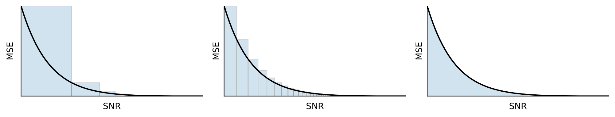
A natural question to ask is what the number of timesteps $T$ should be, and whether more timesteps is always better in terms of the VLB. In Appendix F we analyze the difference between the diffusion loss with $T$ timesteps, $\mathcal{L}T({\mathbf{x}})$, and the diffusion loss with double the timesteps, $\mathcal{L}{2T}({\mathbf{x}})$, while keeping the SNR function fixed. We then find that if our trained denoising model $\hat{{\mathbf{x}}}{{\boldsymbol{\theta}}}$ is sufficiently good, we have that $\mathcal{L}{2T}({\mathbf{x}}) < \mathcal{L}_T({\mathbf{x}})$, i.e. that our VLB will be better for a larger number of timesteps. Intuitively, the discrete time diffusion loss is an upper Riemann sum approximation of an integral of a strictly decreasing function, meaning that a finer approximation yields a lower diffusion loss. This result is illustrated in Figure 2.

5 Continuous-time model: $T\rightarrow\infty$

Section Summary: To improve the model's accuracy, researchers extend the discrete time steps to an infinite number, effectively turning time into a continuous flow described by a diffusion process, much like how particles spread in a fluid. In this setup, the model's training loss simplifies to an integral that measures prediction errors weighted by changes in the signal-to-noise ratio, and it can focus on predicting added noise rather than the original data. Crucially, different ways of defining the diffusion process become equivalent in this continuous limit as long as they share the same noise levels at the start and end, ensuring the generated data distributions remain the same regardless of the details in between; this equivalence even holds for weighted versions of the loss that emphasize noisier data to boost visual quality.

Since taking more time steps leads to a better VLB, we now take $T\rightarrow\infty$, effectively treating time $t$ as continuous rather than discrete. The model for $p({\mathbf{z}}_t)$ can in this case be described as a continuous time diffusion process [5] governed by a stochastic differential equation; see Appendix D. In Appendix E we show that in this limit the diffusion loss $\mathcal{L}_T({\mathbf{x}})$ simplifies further. Letting $\text{SNR}'(t) = d \text{SNR}(t)/dt$, we have, with ${\mathbf{z}}_t = \alpha_t {\mathbf{x}} + \sigma_t {\boldsymbol{\epsilon}}$:

$ \begin{align} \mathcal{L}{\infty}({\mathbf{x}}) &= -\frac{1}{2}\mathbb{E}{{\boldsymbol{\epsilon}}\sim\mathcal{N}(0, \mathbf{I})} \int_{0}^{1} \text{SNR}'(t) \left\rVert {\mathbf{x}} - \hat{{\mathbf{x}}}{{\boldsymbol{\theta}}}({\mathbf{z}}t;t) \right\lVert{2}^{2} dt, \tag{8a} \ &= -\frac{1}{2}\mathbb{E}{{\boldsymbol{\epsilon}}\sim\mathcal{N}(0, \mathbf{I}), t \sim \mathcal{U}(0, 1)} \left[\text{SNR}'(t) \left\rVert {\mathbf{x}} - \hat{{\mathbf{x}}}_{{\boldsymbol{\theta}}}({\mathbf{z}}t;t) \right\lVert{2}^{2} \right]. \tag{8b} \end{align} $

This is the general continuous-time loss for any choice of forward diffusion parameters $(\sigma_t, \alpha_t)$. When plugging in the specifications of $\sigma_t$, $\alpha_t$ and $\hat{{\mathbf{x}}}_{{\boldsymbol{\theta}}}({\mathbf{z}}_t; t)$ that we use in experiments, given in Section 3.2 and Section 3.4, the loss simplifies to:

$ \begin{align} \mathcal{L}{\infty}({\mathbf{x}}) &= \frac{1}{2}\mathbb{E}{{\boldsymbol{\epsilon}}\sim\mathcal{N}(0, \mathbf{I}), t \sim \mathcal{U}(0, 1)} \left[\gamma'{{\boldsymbol{\eta}}}(t) \left\rVert {\boldsymbol{\epsilon}} - \hat{{\boldsymbol{\epsilon}}}{{\boldsymbol{\theta}}}({\mathbf{z}}t;t) \right\lVert{2}^{2} \right], \end{align} $

where $\gamma'{{\boldsymbol{\eta}}}(t) = d \gamma{{\boldsymbol{\eta}}}(t)/dt$. We use the Monte Carlo estimator of this loss for evaluation and optimization.

5.1 Equivalence of diffusion models in continuous time

The signal-to-noise function $\text{SNR}(t)$ is invertible due to the monotonicity assumption in Section 3.1. Due to this invertibility, we can perform a change of variables, and make everything a function of $v \equiv \text{SNR}(t)$ instead of $t$, such that $t = \text{SNR}^{-1}(v)$. Let $\alpha_v$ and $\sigma_v$ be the functions $\alpha_t$ and $\sigma_t$ evaluated at $t = \text{SNR}^{-1}(v)$, and correspondingly let ${\mathbf{z}}v = \alpha_v {\mathbf{x}} + \sigma_v {\boldsymbol{\epsilon}}$. Similarly, we rewrite our noise prediction model as $\tilde{{\mathbf{x}}}{{\boldsymbol{\theta}}}({\mathbf{z}}, v) \equiv \hat{{\mathbf{x}}}_{{\boldsymbol{\theta}}}({\mathbf{z}}, \text{SNR}^{-1}(v))$. With this change of variables, our continuous-time loss in Equation 8a can equivalently be written as:

$ \begin{align} \mathcal{L}{\infty}({\mathbf{x}}) = \frac{1}{2}\mathbb{E}{{\boldsymbol{\epsilon}}\sim\mathcal{N}(0, \mathbf{I})} \int_{\text{SNR}{\text{min}}}^{\text{SNR}{\text{max}}} \left\rVert {\mathbf{x}} - \tilde{{\mathbf{x}}}_{{\boldsymbol{\theta}}}({\mathbf{z}}v, v) \right\lVert{2}^{2} dv, \end{align}\tag{9} $

where instead of integrating w.r.t. time $t$ we now integrate w.r.t. the signal-to-noise ratio $v$, and where $\text{SNR}\text{min}= \text{SNR}(1)$ and $\text{SNR}\text{max}= \text{SNR}(0)$.

What this equation shows us is that the only effect the functions $\alpha(t)$ and $\sigma(t)$ have on the diffusion loss is through the values $\text{SNR}(t) = \alpha^{2}t/\sigma^{2}t$ at endpoints $t=0$ and $t=1$. Given these values $\text{SNR}\text{max}$ and $\text{SNR}\text{min}$, the diffusion loss is invariant to the shape of function $\text{SNR}(t)$ between $t=0$ and $t=1$. The VLB is thus only impacted by the function $\text{SNR}(t)$ through its endpoints $\text{SNR}{\text{min}}$ and $\text{SNR}{\text{max}}$.

Furthermore, we find that the distribution $p({\mathbf{x}})$ defined by our generative model is also invariant to the specification of the diffusion process. Specifically, let $p^{A}({\mathbf{x}})$ denote the distribution defined by the combination of a diffusion specification and denoising function ${\alpha^A_v, \sigma^A_v, \tilde{{\mathbf{x}}}^A_{{\boldsymbol{\theta}}}}$, and similarly let $p^{B}({\mathbf{x}})$ be the distribution defined through a different specification ${\alpha^B_v, \sigma^B_v, \tilde{{\mathbf{x}}}^B_{{\boldsymbol{\theta}}}}$, where both specifications have equal $$\text{SNR}\text{min}, \text{SNR}\text{max}$$; as shown in Appendix G, we then have that $p^{A}({\mathbf{x}}) = p^{B}({\mathbf{x}})$ if $\tilde{{\mathbf{x}}}^B_{{\boldsymbol{\theta}}}({\mathbf{z}}, v) \equiv \tilde{{\mathbf{x}}}^A_{{\boldsymbol{\theta}}}((\alpha^A_v/\alpha^B_v){\mathbf{z}}, v)$. The distribution on all latents ${\mathbf{z}}_v$ is then also the same under both specifications, up to a trivial rescaling. This means that any two diffusion models satisfying the mild constraints set in 3.1 (which includes e.g. the variance exploding and variance preserving specifications considered by [5]), can thus be seen as equivalent in continuous time.

5.2 Weighted diffusion loss

This equivalence between diffusion specifications continues to hold even if, instead of the VLB, these models optimize a weighted diffusion loss of the form:

$ \begin{align} \mathcal{L}{\infty}({\mathbf{x}}, w) = \frac{1}{2}\mathbb{E}{{\boldsymbol{\epsilon}}\sim\mathcal{N}(0, \mathbf{I})} \int_{\text{SNR}{\text{min}}}^{\text{SNR}{\text{max}}} w(v) \left\rVert {\mathbf{x}} - \tilde{{\mathbf{x}}}_{{\boldsymbol{\theta}}}({\mathbf{z}}v, v) \right\lVert{2}^{2} dv, \end{align} $

which e.g. captures all the different objectives discussed by [5], see Appendix K. Here, $w(v)$ is a weighting function that generally puts increased emphasis on the noisier data compared to the VLB, and which thereby can sometimes improve perceptual generation quality as measured by certain metrics like FID and Inception Score. For the models presented in this paper, we further use $w(v)=1$ as corresponding to the (unweighted) VLB.

5.3 Variance minimization

Lowering the variance of the Monte Carlo estimator of the continuous-time loss generally improves the efficiency of optimization. We found that using a low-discrepancy sampler for $t$, as explained in Appendix I.1, leads to a significant reduction in variance. The endpoints of the noise schedule are simply optimized w.r.t. the VLB.

6 Experiments

Section Summary: The experiments evaluate Variational Diffusion Models (VDMs) on popular image datasets like CIFAR-10 and downsampled ImageNet, where the models excel at capturing data patterns by achieving the highest-ever accuracy in likelihood measurements, outperforming prior techniques from methods like VAEs, flows, and other diffusion models. Key results include superior test performance with or without data tweaks, faster training times, and high-quality image samples that rival cutting-edge visuals, even when the focus was on accuracy rather than appearance. Ablation tests confirm that features like continuous-time training, variance reduction, and special signal processing enhancements drive these gains, enabling practical uses such as efficient image compression.

\begin{tabular}{lccccc}
\textbf{Model} & Type & CIFAR10 & CIFAR10 & ImageNet & ImageNet 
\\
(Bits per dim on test set)& & no data aug. & data aug. & 32x32 & 64x64
\\
\midrule
\textit{Previous work}\\
ResNet VAE with IAF [18] & VAE & 3.11 & & & \\
Very Deep VAE [19] & VAE & 2.87 & & 3.80 & 3.52 \\
NVAE [20] & VAE & 2.91 & & 3.92 & \\
Glow [21] & Flow & & $3.35^{(B)}$ & 4.09 & 3.81 \\
Flow++ [22] & Flow & 3.08 & & 3.86 & 3.69 \\
PixelCNN [23] & AR & 3.03 & & 3.83 & 3.57\\
PixelCNN++ [24] & AR & 2.92 & & & \\
Image Transformer [25] & AR & 2.90 & & 3.77 & \\
SPN [26] & AR & & & & 3.52 \\
Sparse Transformer [27]& AR & 2.80 & & & 3.44 
\\
Routing Transformer [28] & AR & & & & 3.43\\
Sparse Transformer + DistAug [29] & AR & & $2.53^{(A)}$ & & \\
DDPM [4] & Diff & & $3.69^{(C)}$ & & 
\\
EBM-DRL [13] & Diff & & $3.18^{(C)}$ & & \\
Score SDE [5] & Diff & 2.99 & & & 
\\
Improved DDPM [6] & Diff & 2.94 & & & 3.54 
\\
\midrule
\textit{Concurrent work}\\
CR-NVAE [30] & VAE & & $2.51^{(A)}$ & & \\ 
LSGM [17] & Diff & 2.87 & & & \\
ScoreFlow [15] (variational bound) & Diff & & $2.90^{(C)}$ & 3.86 & \\
ScoreFlow [15] (cont. norm. flow) & Diff & 2.83 & $2.80^{(C)}$ & 3.76 & \\
\midrule
\textit{Our work}\\
\textbf{VDM (variational bound)} & Diff & \textbf{2.65} & $\textbf{2.49}^{(A)}$ & \textbf{3.72} & \textbf{3.40} 
\\
\bottomrule
\end{tabular}

We demonstrate our proposed class of diffusion models, which we call Variational Diffusion Models (VDMs), on the CIFAR-10 ([31]) dataset, and the downsampled ImageNet ([23, 32]) dataset, where we focus on maximizing likelihood. For our result with data augmentation we used random flips, 90-degree rotations, and color channel swapping. More details of our model specifications are in Appendix B.

6.1 Likelihood and samples

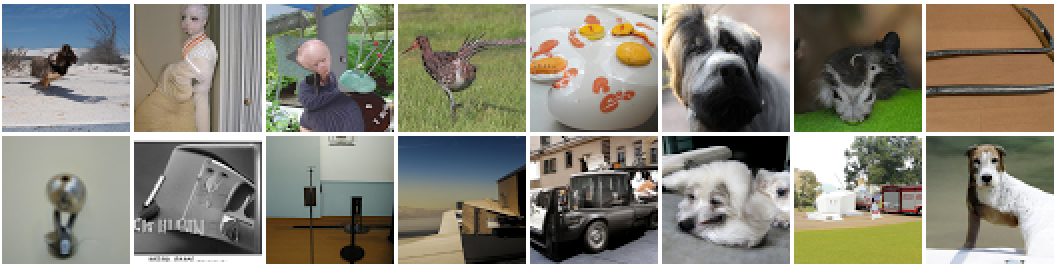
Table 1 shows our results on modeling the CIFAR-10 dataset, and the downsampled ImageNet dataset. We establish a new state-of-the-art in terms of test set likelihood on all considered benchmarks, by a significant margin. Our model for CIFAR-10 without data augmentation surpasses the previous best result of $2.80$ about 10x faster than it takes the Sparse Transformer to reach this, in wall clock time on equivalent hardware. Our CIFAR-10 model, whose hyper-parameters were tuned for likelihood, results in a FID (perceptual quality) score of 7.41. This would have been state-of-the-art until recently, but is worse than recent diffusion models that specifically target FID scores ([6, 5, 4]). By instead using a weighted diffusion loss, with the weighting function $w(\text{SNR})$ used by [4] and described in Appendix K, our FID score improves to 4.0. We did not pursue further tuning of the model to improve FID instead of likelihood. A random sample of generated images from our model is provided in Figure 3. We provide additional samples from this model, as well as our other models for the other datasets, in Appendix M.

6.2 Ablations

Next, we investigate the relative importance of our contributions. In Table 2 we compare our discrete-time and continuous-time specifications of the diffusion model: When evaluating our model with a small number of steps, our discretely trained models perform better by learning the diffusion schedule to optimize the VLB. However, as argued theoretically in Section 4.1, we find experimentally that more steps $T$ indeed gives better likelihood. When $T$ grows large, our continuously trained model performs best, helped by training its diffusion schedule to minimize variance instead.

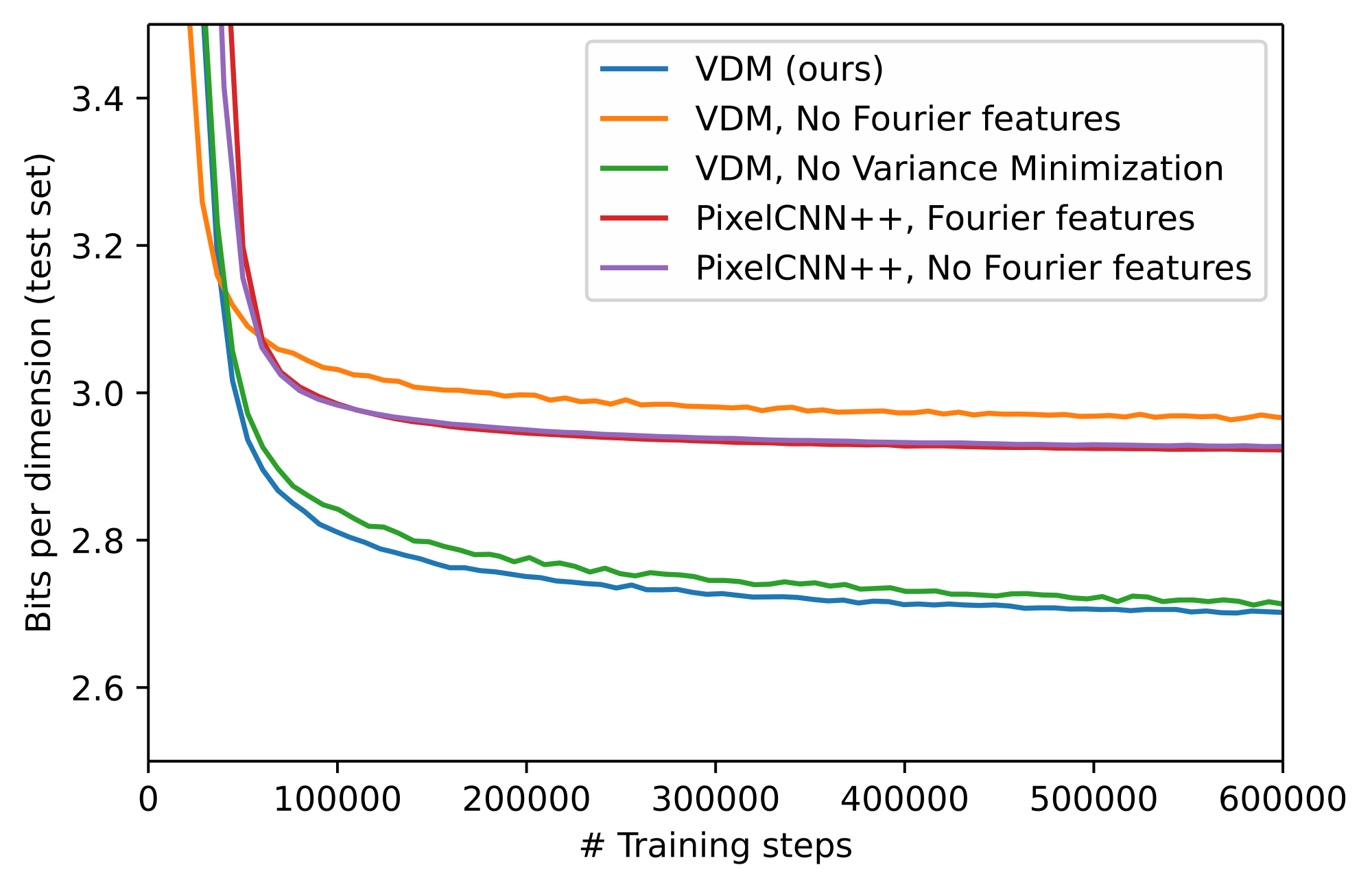
Minimizing the variance also helps the continuous time model to train faster, as shown in Figure 5. This effect is further examined in Table 4b, where we find dramatic variance reductions compared to our baselines in continuous time. Figure 4a shows how this effect is achieved: Compared to the other schedules, our learned schedule spends much more time in the high $\text{SNR}(t)$ / low $\sigma^{2}_{t}$ range.

In Figure 5 we further show training curves for our model including and excluding the Fourier features proposed in Appendix C: with Fourier features enabled our model achieves much better likelihood. For comparison we also implemented Fourier features in a PixelCNN++ model ([24]), where we do not see a benefit. In addition, we find that learning the SNR is necessary to get the most out of including Fourier features: if we fix the SNR schedule to that used by [4], the maximum log-SNR is fixed to approximately 8 (see Figure 7), and test set negative likelihood stays above 4 bits per dim. When learning the SNR endpoints, our maximum log-SNR ends up at $13.3$, which, combined with the inclusion of Fourier features, leads to the SOTA test set likelihoods reported in Table 1.

6.3 Lossless compression

For a fixed number of evaluation timesteps $T_{eval}$, our diffusion model in discrete time is a hierarchical latent variable model that can be turned into a lossless compression algorithm using bits-back coding ([33]). As a proof of concept of practical lossless compression, Table 2 reports net codelengths on the CIFAR10 test set for various settings of $T_{eval}$ using BB-ANS ([34]), an implementation of bits-back coding based on asymmetric numeral systems ([35]). Details of our implementation are given in Appendix N. We achieve state-of-the-art net codelengths, proving our model can be used as the basis of a lossless compression algorithm. However, for large $T_{eval}$ a gap remains with the theoretically optimal codelength corresponding to the negative VLB, and compression becomes computationally expensive due to the large number of neural network forward passes required. Closing this gap with more efficient implementations of bits-back coding suitable for very deep models is an interesting avenue for future work.

\begin{tabular}{rrrc}
$T_{train}$ & $T_{eval}$ & BPD & \makecell{Bits-Back \\ Net BPD} \\
\midrule
10 & 10 & 4.31 & \\
100 & 100 & 2.84 & \\
250 & 250 & 2.73 & \\
500 & 500 & 2.68 & \\
1000 & 1000 & 2.67 & \\
10000 & 10000 & 2.66 & \\
\midrule
$\infty$ & 10 & 7.54 & 7.54 \\
$\infty$ & 100 & 2.90 & 2.91 \\
$\infty$ & 250 & 2.74 & 2.76 \\
$\infty$ & 500 & 2.69 & 2.72 \\
$\infty$ & 1000 & 2.67 & 2.72 \\
$\infty$ & 10000 & \textbf{2.65} & \\
\midrule
$\infty$ & \infty & \textbf{2.65} & \\
\bottomrule
\end{tabular}

7 Conclusion

Section Summary: This research introduces advanced diffusion models that achieve top performance in estimating the density of natural images, featuring customizable diffusion processes, Fourier features for capturing fine details, and other design improvements. It also provides fresh theoretical understanding of these models for generative tasks, revealing that a key evaluation metric remains unchanged regardless of the specific noise-adding process used over time, and demonstrating that several previously distinct diffusion methods are essentially equivalent.

We presented state-of-the-art results on modeling the density of natural images using a new class of diffusion models that incorporates a learnable diffusion specification, Fourier features for fine-scale modeling, as well as other architectural innovations. In addition, we obtained new theoretical insight into likelihood-based generative modeling with diffusion models, showing a surprising invariance of the VLB to the forward time diffusion process in continuous time, as well as an equivalence between various diffusion processes from the literature previously thought to be different.

Acknowledgments

We thank Yang Song, Kevin Murphy, Mohammad Norouzi and Chin-Yun Yu for helpful feedback on the paper, and Ruiqi Gao for helping with writing an open source version of the code.

A Distribution details

Section Summary: This section outlines the key probability distributions in a diffusion model, which gradually adds noise to data and then learns to reverse the process. It details the forward distribution of a noisy state at time t given an earlier state at time s as a Gaussian centered on a scaled version of the earlier state, along with the backward posterior distribution that combines this with the original data to estimate earlier states. Finally, it introduces a model's predicted distribution for reversing noise, interpretable through denoising the data, predicting added noise, or estimating density scores, with practical focus on noise prediction for training.

A.1 $q({\mathbf{z}}_t| {\mathbf{z}}_s)$

The distribution of ${\mathbf{z}}_t$ given ${\mathbf{z}}_s$, for any $0 \leq s < t \leq 1$, is given by:

$ \begin{align} q({\mathbf{z}}_t| {\mathbf{z}}s) = \mathcal{N}\left(\alpha{t|s} {\mathbf{z}}s, \sigma^2{t|s} \mathbf{I}\right), \end{align}\tag{11} $

where

$ \begin{align} \alpha_{t|s} = \alpha_t/\alpha_s, \end{align} $

and

$ \begin{align} \sigma_{t|s}^2 = \sigma_t^2 - \alpha_{t|s}^2\sigma_s^2. \end{align} $

A.2 $q({\mathbf{z}}_s| {\mathbf{z}}_t, {\mathbf{x}})$

Due to the Markov property of the forward process, for $t > s$, we have that $q({\mathbf{z}}_s, {\mathbf{z}}_t | {\mathbf{x}}) = q({\mathbf{z}}_s | {\mathbf{x}}) q({\mathbf{z}}_t | {\mathbf{z}}_s)$. The term $q({\mathbf{z}}_s| {\mathbf{z}}_t, {\mathbf{x}})$ can be viewed as a Bayesian posterior resulting from a prior $q({\mathbf{z}}_s| {\mathbf{x}})$, updated with a likelihood term $q({\mathbf{z}}_t| {\mathbf{z}}_s)$.

Generally, when we have a Gaussian prior of the form $p(x) = \mathcal{N}(\mu_A, \sigma_A^2)$ and a linear-Gaussian likelihood of the form $p(y|x) = \mathcal{N}(a x, \sigma_B^2)$, then the general solution for the posterior is $p(x|y) = \mathcal{N}(\tilde{\mu}, \tilde{\sigma}^2)$, where $\tilde{\sigma}^{-2} = \sigma_A^{-2} + a^2 \sigma_B^{-2}$, and $\tilde{\mu} = \tilde{\sigma}^{-2} (\sigma_A^{-2} \mu_A + a \sigma_B^{-2} y)$.

Plugging our prior term $q({\mathbf{z}}_s| {\mathbf{x}}) = \mathcal{N}\left(\alpha_s {\mathbf{x}}, \sigma^2_s \mathbf{I}\right)$ Equation (1) and linear-Gaussian likelihood term $q({\mathbf{z}}_t| {\mathbf{z}}s) = \mathcal{N}(\alpha{t|s} {\mathbf{z}}s, \sigma^2{t|s})$ Equation (11) into this general posterior equation, yields a posterior:

$ \begin{align} q({\mathbf{z}}s| {\mathbf{z}}t, {\mathbf{x}}) &= \mathcal{N}({\boldsymbol{\mu}}{Q}({\mathbf{z}}{t}, {\mathbf{x}}; s, t), \sigma^2_Q(s, t) \mathbf{I})\ \text{where;;} \sigma^{-2}Q(s, t) &= \sigma_s^{-2} + \alpha{t|s}^{2}\sigma^{-2}{t|s} = \sigma^2_t / (\sigma^2{t|s}\sigma^2_s)\ \sigma^{2}Q(s, t) &= \sigma^2{t|s}\sigma^2_s / \sigma^2_t\ \text{and;;} {\boldsymbol{\mu}}{Q}({\mathbf{z}}{t}, {\mathbf{x}}; s, t) & = \frac{\alpha_{t|s}\sigma^{2}s}{\sigma^{2}t}{\mathbf{z}}{t} + \frac{\alpha_s \sigma^{2}{t|s}}{\sigma^{2}_{t}}{\mathbf{x}}. \end{align}\tag{12} $

A.3 $p({\mathbf{z}}_s| {\mathbf{z}}_t)$

Finally, we choose the conditional model distributions as

$ \begin{align} p({\mathbf{z}}_s| {\mathbf{z}}_t) = q({\mathbf{z}}_s| {\mathbf{z}}t, {\mathbf{x}}=\hat{{\mathbf{x}}}{{\boldsymbol{\theta}}}({\mathbf{z}}_t; t)), \end{align}\tag{13} $

i.e. the same as $q({\mathbf{z}}_s| {\mathbf{z}}t, \mathbf{x})$, but with the original data ${\mathbf{x}}$ replaced by the output of a denoising model $\hat{{\mathbf{x}}}{{\boldsymbol{\theta}}}({\mathbf{z}}_t; t)$ that predicts ${\mathbf{x}}$ from its noisy version ${\mathbf{z}}_t$. We then have

$ \begin{align} p({\mathbf{z}}_s| {\mathbf{z}}t) = \mathcal{N}({\mathbf{z}}s; {\boldsymbol{\mu}}{{\boldsymbol{\theta}}}({\mathbf{z}}{t}; s, t), \sigma^2_Q(s, t) \mathbf{I}) \end{align} $

with variance $\sigma^2_Q(s, t)$ the same as in Equation 12, and

$ \begin{align} {\boldsymbol{\mu}}{{\boldsymbol{\theta}}}({\mathbf{z}}t; s, t) &= \frac{\alpha{t|s}\sigma^{2}s}{\sigma^{2}t}{\mathbf{z}}{t} + \frac{\alpha_s \sigma^{2}{t|s}}{\sigma^{2}{t}}\hat{{\mathbf{x}}}{{\boldsymbol{\theta}}}({\mathbf{z}}t; t) \nonumber\ &= \frac{1}{\alpha{t|s}}{\mathbf{z}}{t} - \frac{\sigma^{2}{t|s}}{\alpha{t|s}\sigma_{t}}\hat{{\boldsymbol{\epsilon}}}{{\boldsymbol{\theta}}}({\mathbf{z}}t; t) \nonumber\ &= \frac{1}{\alpha{t|s}}{\mathbf{z}}t + \frac{\sigma^2{t|s}}{\alpha{t|s}} \mathbf{s}_{{\boldsymbol{\theta}}}({\mathbf{z}}_t;t), \end{align}\tag{14} $

where

$ \begin{align} \hat{{\boldsymbol{\epsilon}}}_{{\boldsymbol{\theta}}}({\mathbf{z}}_t; t) = ({\mathbf{z}}t - \alpha_t\hat{{\mathbf{x}}}{{\boldsymbol{\theta}}}({\mathbf{z}}_t; t))/\sigma_t \end{align} $

and

$ \begin{align} \mathbf{s}_{{\boldsymbol{\theta}}}({\mathbf{z}}t;t) = (\alpha_t\hat{{\mathbf{x}}}{{\boldsymbol{\theta}}}({\mathbf{z}}_t; t) - {\mathbf{z}}_t)/\sigma^{2}_t. \end{align} $

Equation 14 shows that we can interpret our model in three different ways:

1. In terms of the denoising model $\hat{{\mathbf{x}}}_{{\boldsymbol{\theta}}}({\mathbf{z}}_t; t)$ that recovers ${\mathbf{x}}$ from its corrupted version ${\mathbf{z}}_t$.
2. In terms of a noise prediction model $\hat{{\boldsymbol{\epsilon}}}_{{\boldsymbol{\theta}}}({\mathbf{z}}_t; t)$ that directly infers the noise ${\boldsymbol{\epsilon}}$ that was used to generate ${\mathbf{z}}_t$.
3. In terms of a score model $\mathbf{s}_{{\boldsymbol{\theta}}}({\mathbf{z}}_t;t)$, that at its optimum equals the scores of the marginal density: $\mathbf{s}^*({\mathbf{z}}t;t) = \nabla{{\mathbf{z}}} \log q({\mathbf{z}}_t)$; see Appendix L.

These are three equally valid views on the same model class, that have been used interchangeably in the literature. We find the denoising interpretation the most intuitive, and will therefore mostly use $\hat{{\mathbf{x}}}_{{\boldsymbol{\theta}}}({\mathbf{z}}t; t)$ in the theoretical part of this paper, although in practice we parameterize our model via $\hat{{\boldsymbol{\epsilon}}}{{\boldsymbol{\theta}}}({\mathbf{z}}_t; t)$ following [4]. The parameterization of our model is discussed in Appendix B.

A.4 Further simplification of $p({\mathbf{z}}_s| {\mathbf{z}}_t)$

After plugging in the specifications of $\sigma_t$, $\alpha_t$ and $\hat{{\mathbf{x}}}_{{\boldsymbol{\theta}}}({\mathbf{z}}_t; t)$ that we use in experiments, given in Section 3.2 and Section 3.4, it can be verified that the distribution $p({\mathbf{z}}s| {\mathbf{z}}t) = \mathcal{N}({\boldsymbol{\mu}}{{\boldsymbol{\theta}}}({\mathbf{z}}{t}; s, t), \sigma^2_Q(s, t) \mathbf{I})$ simplifies to:

$ \begin{align} {\boldsymbol{\mu}}{{\boldsymbol{\theta}}}({\mathbf{z}}{t}; s, t) &= \frac{\alpha_s}{\alpha_t}\left({\mathbf{z}}t + \sigma_t \text{expm1}(\gamma{{\boldsymbol{\eta}}}(s)-\gamma_{{\boldsymbol{\eta}}}(t)) \hat{{\boldsymbol{\epsilon}}}{{\boldsymbol{\theta}}}({\mathbf{z}}t; t) \right) \ \sigma^2_Q(s, t) &= \sigma^2_s \cdot (- \text{expm1}(\gamma{{\boldsymbol{\eta}}}(s)-\gamma{{\boldsymbol{\eta}}}(t))) \end{align} $

where $\alpha_s = \sqrt{\text{sigmoid}(-\gamma_{{\boldsymbol{\eta}}}(s))}$, $\alpha_t = \sqrt{\text{sigmoid}(-\gamma_{{\boldsymbol{\eta}}}(t))}$, $\sigma^2_s = \text{sigmoid}(\gamma_{{\boldsymbol{\eta}}}(s))$, $\sigma_s = \sqrt{\text{sigmoid}(\gamma_{{\boldsymbol{\eta}}}(s))}$, and where $\text{expm1}(.) = \exp(.)-1$; see Figure 6. Ancestral sampling from this distribution can be performed through simply doing:

$ \begin{align} {\mathbf{z}}_s &= \sqrt{\alpha^2_s/\alpha^2_t}({\mathbf{z}}t - \sigma_t c \hat{{\boldsymbol{\epsilon}}}{{\boldsymbol{\theta}}}({\mathbf{z}}_t; t)) + \sqrt{(1-\alpha^2_s) c} {\boldsymbol{\epsilon}} \end{align} $

where $\alpha^2_s = \text{sigmoid}(-\gamma_{{\boldsymbol{\eta}}}(s))$, $\alpha^2_t = \text{sigmoid}(-\gamma_{{\boldsymbol{\eta}}}(t))$, $c = -\text{expm1}(\gamma_{{\boldsymbol{\eta}}}(s) - \gamma_{{\boldsymbol{\eta}}}(t))$, and ${\boldsymbol{\epsilon}} \sim \mathcal{N}(0, \mathbf{I})$.

B Hyperparameters, architecture, and implementation details

Section Summary: This section outlines the technical setup for the experiments, including shared model designs and training methods, with plans to release the code publicly. The models use a U-Net neural network style to predict noise in data, adapted from prior work by avoiding resizing steps, adding depth and special features for time and input data, limiting attention mechanisms to prevent overfitting, and training with standard optimization techniques on powerful TPU hardware for up to 10 million steps. For specific datasets like CIFAR-10 and ImageNet at various resolutions, the setups vary in network depth, channel counts, batch sizes, and whether data augmentation like flips or rotations is applied to improve performance.

In this section we provide details on the exact setup for each of our experiments. In Appendix B.1 we describe the choices in common to each of our experiments. Hyperparameters specific to the individual experiments are given in Appendix B.2. We are currently working towards open sourcing our code.

B.1 Model and implementation

Our denoising models are parameterized in terms of noise prediction models $\hat{{\boldsymbol{\epsilon}}}{{\boldsymbol{\theta}}}({\mathbf{z}}{t}; \gamma_t)$, as explained in Section 3.4. Our noise prediction models $\hat{{\boldsymbol{\epsilon}}}_{{\boldsymbol{\theta}}}$ closely follow the architecture used by [4], which is based on a U-Net type neural net ([36]) that maps from the input ${\mathbf{z}} \in \mathbb{R}^{d}$ to output of the same dimension. As compared to their publically available code at https://github.com/hojonathanho/diffusion, our implementation differs in the following ways:

• Our networks don't perform any internal downsampling or upsampling: we process all the data at the original input resolution.
• Our models are deeper than those used by [4]. Specific numbers are given in Appendix B.2.
• Instead of taking time $t$ as input to the noise prediction model, we use $\gamma_t$, which we rescale to have approximately the same range as $t$ of $[0, 1]$ before using it to form 'time' embeddings in the same way as Ho et al. [4].
• Our models calculate Fourier features on the input data ${\mathbf{z}}_t$ as discussed in Appendix C, which are then concatenated to ${\mathbf{z}}_t$ before being fed to the U-Net.
• Apart from the middle attention block that connects the upward and downward branches of the U-Net, we remove all other attention blocks from the model. We found that these attention blocks made it more likely for the model to overfit to the training set.
• All of our models use dropout at a rate of 0.1 in the intermediate layers, as did Ho et al. [4]. In addition we regularize the model by using decoupled weight decay ([37]) with coefficient 0.01.
• We use the Adam optimizer with a learning rate of $2e^{-4}$ and exponential decay rates of $\beta_{1}=0.9, \beta_{2}=0.99$. We found that higher values for $\beta_{2}$ resulted in training instabilities.
• For evaluation, we use an exponential moving average of our parameters, calculated with an exponential decay rate of $0.9999$.

We regularly evaluate the variational bound on the likelihood on the validation set and find that our models do not overfit during training, using the current settings. We therefore do not use early stopping and instead allow the network to be optimized for 10 million parameter updates for CIFAR-10, and for 2 million updates for ImageNet, before obtaining the test set numbers reported in this paper. It looks like our models keep improving even after this number of updates, in terms of likelihood, but we did not explore this systematically due to resource constraints.

All of our models are trained on TPUv3 hardware (see https://cloud.google.com/tpu) using data parallelism. We also evaluated our trained models using CPU and GPU to check for robustness of our reported numbers to possible rounding errors. We found only very small differences when evaluating on these other hardware platforms.

B.2 Settings for each dataset

Our model for CIFAR-10 with no data augmentation uses a U-Net of depth 32, consisting of 32 ResNet blocks in the forward direction and 32 ResNet blocks in the reverse direction, with a single attention layer and two additional ResNet blocks in the middle. We keep the number of channels constant throughout at 128. This model was trained on 8 TPUv3 chips, with a total batch size of 128 examples. Reaching a test-set BPD of $2.65$ after 10 million updates takes 9 days, although our model already surpasses sparse transformers (the previous state-of-the-art) of $2.80$ BPD after only $2.5$ hours of training.

For CIFAR-10 with data augmentation we used random flips, 90-degree rotations, and color channel swapping, which were previously shown to help for density estimation by Jun et al. [29]. Each of the three augmentations independently were given a $50%$ probability of being applied to each example, which means that 1 in 8 training examples was not augmented at all. For this experiment, we doubled the number of channels in our model to 256, and decreased the dropout rate from $10%$ to $5%$. Since overfitting was less of a problem with data augmentation, we add back the attention blocks after each ResNet block, following Ho et al. [4]. We also experimented with conditioning our model on an additional binary feature that indicates whether or not the example was augmented, which can be seen as a simplified version of the augmentation conditioning proposed by Jun et al. [29]. Conditioning made almost no difference to our results, which may be explained by the relatively large fraction ($12.5%$) of clean data fed to our model during training. We trained our model for slightly over a week on 128 TPUv3 chips to obtain the reported result.

Our model for 32x32 ImageNet looks similar to that for CIFAR-10 without data augmentation, with a U-Net depth of 32, but uses double the number of channels at 256. It is trained using data parallelism on 32 TPUv3 chips, with a total batch size of 512.

Our model for 64x64 ImageNet uses double the depth at 64 ResNet layers in both the forward and backward direction in the U-Net. It also uses a constant number of channels of 256. This model is trained on 128 TPUv3 chips at a total batch size of 512 examples.

C Fourier features for improved fine scale prediction

Section Summary: Previous research on diffusion models prioritized the overall look and big-picture consistency of generated images, but this approach focuses on precise pixel-level details to improve accuracy in predictions. To handle these fine details, especially at low noise levels where the discrete nature of image data creates sharp patterns, the model incorporates Fourier features—high-frequency sine and cosine transformations of the input values added as extra channels. This enhancement allows the network to learn better at lower noise levels, significantly boosting prediction accuracy without similar gains in other model types.

Prior work on diffusion models has mainly focused on the perceptual quality of generated samples, which emphasizes coarse scale patterns and global consistency of generated images. Here, we optimize for likelihood, which is sensitive to fine scale details and exact values of individual pixels. Since our reconstruction model $p({\mathbf{x}}| {\mathbf{z}}{0})$ given in Equation 2 is weak, the burden of modeling these fine scale details falls on our denoising diffusion model $\hat{{\mathbf{x}}}{{\boldsymbol{\theta}}}$. In initial experiments, we found that the denoising model had a hard time accurately modeling these details. At larger noise levels, the latents ${\mathbf{z}}_t$ follow a smooth distribution due to the added Gaussian noise, but at the smallest noise levels the discrete nature of 8-bit image data leads to sharply peaked marginal distributions $q({\mathbf{z}}_t)$.

To capture the fine scale details of the data, we propose adding a set of Fourier features to the input of our denoising model $\hat{{\mathbf{x}}}_{{\boldsymbol{\theta}}}({\mathbf{z}}_t; t)$. Such Fourier features consist of a linear projection of the original data onto a set of periodic basis functions with high frequency, which allows the network to more easily model high frequency details of the data. Previous work [38] has used these features for input coordinates to model high frequency details across the spatial dimension, and for time embeddings to condition denoising networks over the temporal dimension ([5]). Here we apply it to color channels for single pixels, in order to model fine distributional details at the level of each scalar input.

Concretely, let $z_{i, j, k}$ be the scalar value in the $k$-th channel in the $(i, j)$ spatial position of network input ${\mathbf{z}}_t$. We then add additional channels to the input of the denoising model of the form

$ \begin{align} f^{n}{i, j, k} = \sin(z{i, j, k}2^{n}\pi), \text{;;and;;} g^{n}{i, j, k} = \cos(z{i, j, k}2^{n}\pi), \end{align} $

where $n$ runs over a range of integers ${n_{min}, ..., n_{max}}$. These additional channels are then concatenated to ${\mathbf{z}}t$ before being used as input in a standard convolutional denoising model similar to that used by Ho et al. [4]. We find that the presence of these high frequency features allows our network to learn with much higher values of $\text{SNR}{\text{max}}$, or conversely lower noise levels $\sigma^{2}_{0}$, than is otherwise optimal. This leads to large improvements in likelihood as demonstrated in Section 6 and Figure 5. We did not observe such improvements when incorporating Fourier features into autoregressive models.

In our expreriments, we got best results with $n_{min}=7$ and $n_{max}=8$, probably since Fourier features with these frequencies are most relevant; features with lower frequencies can be learned by the network from ${\mathbf{z}}$, and higher frequencies are not present in the data thus irrelevant for likelihood.

D As a SDE

Section Summary: As the number of steps in the model increases indefinitely, the probability distribution for the variable z at time t evolves as a continuous diffusion process, much like a gradual random spread over time. This process is captured by a stochastic differential equation that describes how z changes: it includes a drift term pulling it toward a learned direction based on a function s, plus random noise from a Wiener process, all while time flows backward from 1 to 0.

When we take the number of steps $T\rightarrow\infty$, our model for $p({\mathbf{z}}_t)$ can best be described as a continuous time diffusion process ([5]), governed by the stochastic differential equation

$ \begin{align} d {\mathbf{z}}t = [f(t){\mathbf{z}}{t} - g^{2}(t)s_{{\boldsymbol{\theta}}}({\mathbf{z}}t; t)] dt + g(t)d {\mathbf{W}}{t}, \end{align} $

with time running backwards from $t=1$ to $t=0$, where ${\mathbf{W}}$ denotes a Wiener process.

E Derivation of the VLB estimators

Section Summary: This section derives practical ways to compute the Variational Lower Bound (VLB), a key approximation used in training diffusion models that generate data by reversing a noise-adding process. It decomposes the VLB into three parts—prior loss, reconstruction loss, and diffusion loss—and focuses on simplifying the diffusion loss into a formula involving signal-to-noise ratios and the squared error between original and predicted data. For efficiency, it introduces an unbiased estimator by randomly sampling time steps instead of calculating every one, and discusses how this extends to a continuous version when the number of steps grows infinite.

E.1 Discrete-time VLB

Similar to [9], we decompose the negative variational lower bound (VLB) as:

$ \begin{align}

• \log p({\mathbf{x}}) \leq
  • \text{VLB}({\mathbf{x}}) = \underbrace{ D_{KL}(q({\mathbf{z}}_1| {\mathbf{x}})||p({\mathbf{z}}1)) }{\text{Prior loss}}
  • \underbrace{ \mathbb{E}_{q({\mathbf{z}}_0| {\mathbf{x}})}\left[- \log p({\mathbf{x}}| {\mathbf{z}}0) \right] }{\text{Reconstruction loss}}
  • \underbrace{ \mathcal{L}T({\mathbf{x}}). }{\text{Diffusion loss}} \end{align} $

The prior loss and reconstruction loss can be (stochastically and differentiably) estimated using standard techniques. We will now derive an estimator for the diffusion loss $\mathcal{L}_T({\mathbf{x}})$, the remaining and more challenging term. In the case of finite $T$, using $s(i) = (i-1)/T$, $t(i) = i/T$, the diffusion loss is:

$ \begin{align} \mathcal{L}T({\mathbf{x}}) &= \sum{i=1}^T \mathbb{E}{q({\mathbf{z}}{t(i)}| {\mathbf{x}})} D_{KL}[q({\mathbf{z}}{s(i)}| {\mathbf{z}}{t(i)}, {\mathbf{x}})||p({\mathbf{z}}{s(i)}| {\mathbf{z}}{t(i)})]. \end{align} $

We will use $s$ and $t$ as shorthands for $s(i)$ and $t(i)$. We will first derive an expression of $D_{KL}(q({\mathbf{z}}_s| {\mathbf{z}}_t, {\mathbf{x}})||p({\mathbf{z}}_s| {\mathbf{z}}_t))$.

Recall that $p({\mathbf{z}}_s| {\mathbf{z}}_t) = q({\mathbf{z}}_s| {\mathbf{z}}t, {\mathbf{x}}=\hat{{\mathbf{x}}}{{\boldsymbol{\theta}}}({\mathbf{z}}_t; t))$, and thus $q({\mathbf{z}}_s| {\mathbf{z}}t, {\mathbf{x}}) = \mathcal{N}({\mathbf{z}}s; {\boldsymbol{\mu}}{Q}({\mathbf{z}}{t}, {\mathbf{x}}; s, t), \sigma^2_Q(s, t) \mathbf{I})$ and $p({\mathbf{z}}_s| {\mathbf{z}}t) = \mathcal{N}({\mathbf{z}}s; {\boldsymbol{\mu}}{{\boldsymbol{\theta}}}({\mathbf{z}}{t}; s, t), \sigma^2_Q(s, t) \mathbf{I})$, with

$ \begin{align} {\boldsymbol{\mu}}{Q}({\mathbf{z}}t, {\mathbf{x}}; s, t) &= \frac{\alpha{t|s}\sigma^{2}s}{\sigma^{2}t}{\mathbf{z}}{t} + \frac{\alpha_s \sigma^{2}{t|s}}{\sigma^{2}{t}}{\mathbf{x}}\ {\boldsymbol{\mu}}{{\boldsymbol{\theta}}}({\mathbf{z}}t; s, t) &= \frac{\alpha{t|s}\sigma^{2}s}{\sigma^{2}t}{\mathbf{z}}{t} + \frac{\alpha_s \sigma^{2}{t|s}}{\sigma^{2}{t}}\hat{{\mathbf{x}}}_{{\boldsymbol{\theta}}}({\mathbf{z}}t; t), \ \text{and;;} \sigma^2_Q(s, t) &= \sigma^2{t|s}\sigma^2_s / \sigma^2_t. \end{align} $

Since $q({\mathbf{z}}_s| {\mathbf{z}}_t, {\mathbf{x}})$ and $p({\mathbf{z}}_s| {\mathbf{z}}_t)$ are Gaussians, their KL divergence is available in closed form as a function of their means and variances, which due to their with equal variances simplifies as:

$ \begin{align} D_{KL}(q({\mathbf{z}}_s| {\mathbf{z}}_t, {\mathbf{x}})||p({\mathbf{z}}_s| {\mathbf{z}}_t)) &= \frac{1}{2\sigma^2_Q(s, t)} || {\boldsymbol{\mu}}Q - {\boldsymbol{\mu}}{\boldsymbol{\theta}}||_2^2

\ &= \frac{\sigma^2_t}{2\sigma^2_{t|s}\sigma^2_s} \frac{\alpha_s^{2} \sigma^{4}{t|s}}{\sigma^{4}{t}} || {\mathbf{x}} - \hat{{\mathbf{x}}}{{\boldsymbol{\theta}}}({\mathbf{z}}t; t)||2^2\ &= \frac{1}{2\sigma^2_s} \frac{\alpha_s^{2} \sigma^{2}{t|s}}{\sigma^{2}{t}} || {\mathbf{x}} - \hat{{\mathbf{x}}}{{\boldsymbol{\theta}}}({\mathbf{z}}_t; t)||2^2\ &= \frac{1}{2\sigma^2_s} \frac{\alpha_s^{2}(\sigma^{2}t - \alpha{t|s}^{2}\sigma^{2}s)}{\sigma^{2}{t}} || {\mathbf{x}} - \hat{{\mathbf{x}}}{{\boldsymbol{\theta}}}({\mathbf{z}}t; t)||2^2\ &= \frac{1}{2} \frac{\alpha_s^{2}\sigma^{2}t/\sigma^2_s - \alpha{t}^{2}}{\sigma^{2}{t}} || {\mathbf{x}} - \hat{{\mathbf{x}}}{{\boldsymbol{\theta}}}({\mathbf{z}}_t; t)||_2^2\ &= \frac{1}{2}\left(\frac{\alpha_s^{2}}{\sigma^2_s} - \frac{\alpha_t^{2}}{\sigma^{2}t}\right) || {\mathbf{x}} - \hat{{\mathbf{x}}}{{\boldsymbol{\theta}}}({\mathbf{z}}_t; t)||2^2\ &= \frac{1}{2}\left(\text{SNR}(s) - \text{SNR}(t)\right) || {\mathbf{x}} - \hat{{\mathbf{x}}}{{\boldsymbol{\theta}}}({\mathbf{z}}_t; t)||_2^2 \end{align}\tag{15} $

Reparameterizing ${\mathbf{z}}_t \sim q({\mathbf{z}}_t| {\mathbf{x}})$ as ${\mathbf{z}}_t = \alpha_t {\mathbf{x}} + \sigma_t {\boldsymbol{\epsilon}}$, where ${\boldsymbol{\epsilon}} \sim \mathcal{N}(0, \mathbf{I})$, our diffusion loss becomes:

$ \begin{align} \mathcal{L}T({\mathbf{x}}) &= \sum{i=1}^T \mathbb{E}_{q({\mathbf{z}}t| {\mathbf{x}})}[D{KL}(q({\mathbf{z}}_s| {\mathbf{z}}t, {\mathbf{x}})||p({\mathbf{z}}s| {\mathbf{z}}t))]\ &= \frac{1}{2}\mathbb{E}{{\boldsymbol{\epsilon}} \sim \mathcal{N}(0, \mathbf{I})}[\sum{i=1}^T \left(\text{SNR}(s) - \text{SNR}(t)\right) || {\mathbf{x}} - \hat{{\mathbf{x}}}{{\boldsymbol{\theta}}}({\mathbf{z}}_t; t)||_2^2] \end{align} $

E.2 Estimator of $\mathcal{L}_T({\mathbf{x}})$

To avoid having to compute all $T$ terms when calculating the diffusion loss, we construct an unbiased estimator of $\mathcal{L}_T({\mathbf{x}})$ using

$ \begin{align} \mathcal{L}T({\mathbf{x}}) = \frac{T}{2} \mathbb{E}{{\boldsymbol{\epsilon}} \sim \mathcal{N}(0, \mathbf{I}), i \sim U{1, T}} \left[\left(\text{SNR}(s)-\text{SNR}(t)\right) || {\mathbf{x}} - \hat{{\mathbf{x}}}_{{\boldsymbol{\theta}}}({\mathbf{z}}_t;t) ||_2^2 \right] \end{align} $

where $U{1, T}$ is the discrete uniform distribution from $1$ to (and including) $T$, $s = (i-1)/T$, $t = i/T$ and ${\mathbf{z}}_t = \alpha_t {\mathbf{x}} + \sigma_t {\boldsymbol{\epsilon}}$. This trivially yields an unbiased Monte Carlo estimator, by drawing random samples $i \sim U{1, T}$ and ${\boldsymbol{\epsilon}} \sim \mathcal{N}(0, \mathbf{I})$.

E.3 Infinite depth ($T \to \infty$)

To calculate the limit of the diffusion loss as $T\rightarrow\infty$, we express $\mathcal{L}_T({\mathbf{x}})$ as a function of $\tau = 1/T$:

$ \begin{align} \mathcal{L}T({\mathbf{x}}) = \frac{1}{2} \mathbb{E}{{\boldsymbol{\epsilon}} \sim \mathcal{N}(0, \mathbf{I}), i \sim U{1, T}} \left[\frac{\text{SNR}(t-\tau)-\text{SNR}(t)}{\tau} || {\mathbf{x}} - \hat{{\mathbf{x}}}_{{\boldsymbol{\theta}}}({\mathbf{z}}_t;t) ||_2^2 \right], \end{align} $

where again $t = i/T$ and ${\mathbf{z}}_t = \alpha_t {\mathbf{x}} + \sigma_t {\boldsymbol{\epsilon}}$.

As $\tau \rightarrow 0, T \rightarrow \infty$, and letting $\text{SNR}'(t)$ denote the derivative of the SNR function, this then gives

$ \begin{align} \mathcal{L}{\infty}({\mathbf{x}}) &= -\frac{1}{2} \mathbb{E}{{\boldsymbol{\epsilon}} \sim \mathcal{N}(0, \mathbf{I}), t \sim U[0, 1]} \left[\text{SNR}'(t)|| {\mathbf{x}} - \hat{{\mathbf{x}}}{{\boldsymbol{\theta}}}({\mathbf{z}}t;t) ||2^2 \right]\ &= -\frac{1}{2}\mathbb{E}{{\boldsymbol{\epsilon}}\sim\mathcal{N}(0, \mathbf{I})} \int{0}^{1} \text{SNR}'(t) \left\rVert {\mathbf{x}} - \hat{{\mathbf{x}}}{{\boldsymbol{\theta}}}({\mathbf{z}}t;t) \right\lVert{2}^{2} dt . \end{align} $

F Influence of the number of steps $T$ on the VLB

Section Summary: The section explains how increasing the number of steps, or timesteps, in a diffusion model affects its training loss, showing through equations that doubling the steps from T to 2T always lowers the loss. This improvement happens because, with more steps, the model often predicts the original data from versions that are less corrupted by noise, making the task easier and leading to better accuracy. As a result, the authors recommend using a continuous-time approach, which is like taking an infinite number of steps, to achieve the best possible performance.

Recall that the diffusion loss for our choice of model $p, q$, when using $T$ timesteps, is given by

$ \begin{align} \mathcal{L}T({\mathbf{x}}) = \frac{1}{2}\mathbb{E}{{\boldsymbol{\epsilon}} \sim \mathcal{N}(0, \mathbf{I})} \left[\sum_{i=1}^T \left(\text{SNR}(s(i))- \text{SNR}(t(i))\right) || {\mathbf{x}} - \hat{{\mathbf{x}}}{{\boldsymbol{\theta}}}({\mathbf{z}}{t(i)};t(i)) ||_2^2 \right], \end{align} $

with $s(i) = (i-1)/T$, $t(i) = i/T$.

This can then be written equivalently as

$ \begin{align} \mathcal{L}T({\mathbf{x}}) = \frac{1}{2}\mathbb{E}{{\boldsymbol{\epsilon}} \sim \mathcal{N}(0, \mathbf{I})} \left[\sum_{i=1}^T \left(\text{SNR}(s)- \text{SNR}(t') + \text{SNR}(t')- \text{SNR}(t)\right) || {\mathbf{x}} - \hat{{\mathbf{x}}}{{\boldsymbol{\theta}}}({\mathbf{z}}{t};t) ||_2^2 \right], \end{align} $

with $t' = t - 0.5/T$.

In contrast, the diffusion loss with 2T timesteps can be written as

$ \begin{align} \mathcal{L}{2T}({\mathbf{x}}) = \frac{1}{2}\mathbb{E}{{\boldsymbol{\epsilon}} \sim \mathcal{N}(0, \mathbf{I})} & \sum_{i=1}^T \left(\text{SNR}(s)- \text{SNR}(t')\right) || {\mathbf{x}} - \hat{{\mathbf{x}}}{{\boldsymbol{\theta}}}({\mathbf{z}}{t'};t') ||2^2 \nonumber\ &+ \sum{i=1}^T \left(\text{SNR}(t')- \text{SNR}(t)\right) || {\mathbf{x}} - \hat{{\mathbf{x}}}{{\boldsymbol{\theta}}}({\mathbf{z}}{t};t) ||_2^2. \end{align} $

Subtracting the two results, we get

$ \begin{align} & \mathcal{L}{2T}({\mathbf{x}}) - \mathcal{L}T({\mathbf{x}}) = \nonumber\ &\frac{1}{2}\mathbb{E}{{\boldsymbol{\epsilon}} \sim \mathcal{N}(0, \mathbf{I})} \left[\sum{i=1}^T (\text{SNR}(s)- \text{SNR}(t')) \left(|| {\mathbf{x}} - \hat{{\mathbf{x}}}{{\boldsymbol{\theta}}}({\mathbf{z}}{t'};t') ||2^2 - || {\mathbf{x}} - \hat{{\mathbf{x}}}{{\boldsymbol{\theta}}}({\mathbf{z}}_{t};t) ||_2^2 \right)\right]. \end{align} $

Since $t' < t$, ${\mathbf{z}}{t'}$ is a less noisy version of the data from earlier in the diffusion process compared to ${\mathbf{z}}{t}$. Predicting the original data ${\mathbf{x}}$ from ${\mathbf{z}}{t'}$ is thus strictly easier than from ${\mathbf{z}}{t}$, leading to lower mean squared error if our model $\hat{\mathbf{x}}{{\boldsymbol{\theta}}}$ is good enough. We thus have that $\mathcal{L}{2T}({\mathbf{x}}) - \mathcal{L}_T({\mathbf{x}}) < 0$, which means that doubling the number of timesteps always improves our diffusion loss. For this reason we argue for using the continuous-time VLB corresponding to $T\rightarrow\infty$ in this paper.

G Equivalence of diffusion specifications

Section Summary: Different ways of defining how noise is added to data in diffusion models, such as varying the scaling factors alpha and sigma, turn out to be equivalent because the noisy versions of the data, known as latents, are identical up to a simple rescaling based on their signal-to-noise ratio. This means that by tweaking the denoising function to account for the scaling, models using different specifications achieve the same accuracy in reconstructing the original data and the same overall training loss. As a result, all these approaches generate new data in fundamentally the same way, differing only in the scale of the intermediate noisy steps.

(Continuation of Section 5.1.)

Let $p^{A}({\mathbf{x}})$ denote the distribution on observed data ${\mathbf{x}}$ as defined by the combination of a diffusion specification ${\alpha^A_v, \sigma^A_v}$ and denoising function $\tilde{{\mathbf{x}}}^A_{{\boldsymbol{\theta}}}$, and let ${\mathbf{z}}^{A}_v$ denote the latents of this diffusion process. Similarly, let $p^{B}({\mathbf{x}}), {\mathbf{z}}^{B}v$ be defined through a different specification ${\alpha^B_v, \sigma^B_v, \tilde{{\mathbf{x}}}^B{{\boldsymbol{\theta}}}}$.

Since $v \equiv \alpha_v^2/\sigma_v^2$, we have that $\sigma_v = \alpha_v/\sqrt{v}$, which means that ${\mathbf{z}}_v({\mathbf{x}}, {\boldsymbol{\epsilon}}) = \alpha_v {\mathbf{x}} + \sigma_v {\boldsymbol{\epsilon}} = \alpha_v({\mathbf{x}} + {\boldsymbol{\epsilon}}/\sqrt{v})$. This holds for any diffusion specification by definition, and therefore we have ${\mathbf{z}}^A_v({\mathbf{x}}, {\boldsymbol{\epsilon}}) = (\alpha^A_v/\alpha^B_v) {\mathbf{z}}_v^B({\mathbf{x}}, {\boldsymbol{\epsilon}})$. The latents ${\mathbf{z}}_v$ for different diffusion specifications are thus identical, up to a trivial rescaling, and their information content only depends on the signal-to-noise ratio $v$, not on $\alpha_v, \sigma_v$ separately.

For the purpose of denoising from a latent ${\mathbf{z}}^{B}{v}$, this means we can simply define the denoising model as $\tilde{{\mathbf{x}}}^B{{\boldsymbol{\theta}}}({\mathbf{z}}^{B}{v}, v) \equiv \tilde{{\mathbf{x}}}^A{{\boldsymbol{\theta}}}((\alpha^A_v/\alpha^B_v){\mathbf{z}}^{B}{v}, v)$, and we will then get the same reconstruction loss as when denoising from ${\mathbf{z}}^{A}{v}$ using model $\tilde{{\mathbf{x}}}^A_{{\boldsymbol{\theta}}}$. Assuming endpoints $\text{SNR}{\text{max}}$ and $\text{SNR}{\text{min}}$ are equal for both specifications, Equation 9 then tells us that $\mathcal{L}^A_{\infty}({\mathbf{x}}) = \mathcal{L}^B_{\infty}({\mathbf{x}})$, i.e. they both produce the same diffusion loss in continuous time.

Similarly, the conditional model distributions over the latents ${\mathbf{z}}{v}$ in our generative model are functions of the denoising model $\tilde{{\mathbf{x}}}{{\boldsymbol{\theta}}}({\mathbf{z}}{v}, v)$ (see Equation 13), and we therefore have that the specification ${\alpha^A_v, \sigma^A_v, \tilde{{\mathbf{x}}}^A{{\boldsymbol{\theta}}}}$ defines the same generative model over ${\mathbf{z}}{v}, {\mathbf{x}}$ as the specification ${\alpha^B_v, \sigma^B_v, \tilde{{\mathbf{x}}}^B{{\boldsymbol{\theta}}}}$, again up to a rescaling of the latents by $\alpha^A_v/\alpha^B_v$.

H Implementation of monotonic neural net noise schedule $\gamma_{\eta}(t)$

Section Summary: To create a smoothly changing noise schedule for their model, the researchers define the signal-to-noise ratio as an exponential function of a special neural network output called γ_η(t), which is designed to always increase steadily. This network uses three layers of simple linear calculations with positive weights only, structured so the input time t flows through the first layer, then a wide middle layer with 1024 connections activated by a sigmoid function, and finally added to outputs from the first and third layers. For the continuous-time version, they refine this schedule afterward to minimize variations in noise, as explained in an appendix.

To learn the signal-to-noise ratio $\text{SNR}(t)$, we parameterize it as $\text{SNR}(t) = \exp(-\gamma_{{\boldsymbol{\eta}}}(t))$ with $\gamma_{{\boldsymbol{\eta}}}(t)$ a monotonic neural network. This network consists of 3 linear layers with weights that are restricted to be positive, $l_{1}, l_{2}, l_{3}$, which are composed as $\tilde{\gamma}{{\boldsymbol{\eta}}}(t) = l{1}(t)+l_{3}(\phi(l_{2}(l_{1}(t))))$, with $\phi$ the sigmoid function. Here, the $l_2$ layer has 1024 outputs, and the other layers have a single output.

In case of the continuous-time model, for the purpose of variance minimization, we postprocess the noise schedule as detailed in Appendix I.

I Variance minimization

Section Summary: Reducing the variance in the diffusion loss estimator helps speed up the optimization process in this continuous-time model. One approach uses a low-discrepancy sampler to spread out the timesteps more evenly across a batch of examples, ensuring better coverage and lowering variance in the estimate without independent random sampling. The other method fine-tunes the noise schedule by optimizing its parameters to minimize the variance of the loss through a post-processing step and efficient gradient calculations, though both techniques are optional for simpler setups at the cost of slower training.

Reduction of the variance diffusion loss estimator can lead to faster optimization.

For the continuous-time model, we reduce the variance of the diffusion loss estimator through two methods: (1) optimizing the noise schedule w.r.t. the variance of the diffusion loss, and (2) using a low-discrepancy sampler. Note that these methods can be omitted if one aims for a simple implementation of our methods, at the expense of slower optimization.

I.1 Low-discrepancy sampler

When processing a minibatch of $k$ examples ${\mathbf{x}}^{i}$, $i \in {1, \ldots, k}$, we require $k$ timesteps $t^{i}$ sampled from a uniform distribution. Instead of sampling these timesteps independently, we sample a single uniform random number $u_{0} \sim U[0, 1]$ and then set $t^{i} = \text{mod}(u_{0} + i/k, 1)$. Each $t^{i}$ now has the correct uniform marginal distribution, but the minibatch of timesteps covers the space in $[0, 1]$ more equally than when sampling independently, which we find to reduce the variance in our VLB estimate.

I.2 Optimizing the noise schedule w.r.t. the variance of the diffusion loss

In case of the continuous-time model, for the purpose of variance minimization, we postprocess the noise schedule as follows. At this point, the range of $\tilde{\gamma}{{\boldsymbol{\eta}}}(t)$ is unbounded and so the resulting $\text{SNR}$ is not yet restricted to $[\text{SNR}{\text{min}}, \text{SNR}_{\text{max}}]$. We therefore postprocess the monotonic neural network as

$ \begin{align} \gamma_{{\boldsymbol{\eta}}}(t) = \gamma_0 + (\gamma_1 - \gamma_0)\frac{\tilde{\gamma}{{\boldsymbol{\eta}}}(t) - \tilde{\gamma}{{\boldsymbol{\eta}}}(0)}{\tilde{\gamma}{{\boldsymbol{\eta}}}(1) - \tilde{\gamma}{{\boldsymbol{\eta}}}(0)}, \end{align} $

with $\gamma_0 = -\log(\text{SNR}{\text{max}}), \gamma_1 = -\log(\text{SNR}{\text{min}})$. Now $\text{SNR}(t) = \exp(-\gamma_{{\boldsymbol{\eta}}}(t))$ has the correct range and interpolates exactly between $\text{SNR}{\text{min}}$ and $\text{SNR}{\text{max}}$. We treat $\gamma_0, \gamma_1$ as free parameters that we optimize directly w.r.t. the VLB. The remaining parameters ${\boldsymbol{\eta}}$ are instead learned by minimizing the variance of the stochastic estimate of the VLB.

We minimize the variance by performing stochastic gradient descent on our squared diffusion loss $\mathcal{L}^{MC}{\infty}({\mathbf{x}}, w, \gamma)^{2}$. We have that $\mathbb{E}{t, {\boldsymbol{\epsilon}}}[\mathcal{L}^{MC}{\infty}({\mathbf{x}}, w, \gamma)^{2}] = \mathcal{L}{\infty}({\mathbf{x}}, w)^{2} + \mathrm{Var}{t, {\boldsymbol{\epsilon}}}[\mathcal{L}^{MC}{\infty}({\mathbf{x}}, w, \gamma)]$, where the first part is independent of $\gamma_{{\boldsymbol{\eta}}}(t)$, and hence that

$ \begin{align} \mathbb{E}{t, {\boldsymbol{\epsilon}}}[\nabla{{\boldsymbol{\eta}}} \mathcal{L}^{MC}{\infty}({\mathbf{x}}, w, \gamma{{\boldsymbol{\eta}}})^{2}] = \nabla_{{\boldsymbol{\eta}}} \mathrm{Var}{t, {\boldsymbol{\epsilon}}}[\mathcal{L}^{MC}{\infty}({\mathbf{x}}, w, \gamma_{{\boldsymbol{\eta}}})]. \end{align} $

We can calculate this gradient with negligible computational overhead as a by-product of calculating the gradient of the VLB, details of which are given in Appendix H.

We wish to calculate $\nabla_{{\boldsymbol{\eta}}}[\mathcal{L}^{MC}{\infty}({\mathbf{x}}, \gamma{{\boldsymbol{\eta}}})^{2}]$ without performing a second backpropagation pass through the denoising model due to this objective being different than for the other parameters. To do this, we decompose the gradient as

$ \begin{align} \frac{d}{d {\boldsymbol{\eta}}}[\mathcal{L}^{MC}{\infty}({\mathbf{x}}, \gamma{{\boldsymbol{\eta}}})^{2}] &= \frac{d}{d \text{SNR}}\left[\mathcal{L}^{MC}{\infty}({\mathbf{x}}, \text{SNR})^{2}\right]\frac{d}{d {\boldsymbol{\eta}}}\left[\text{SNR}({\boldsymbol{\eta}})\right], \ \text{and;;} \frac{d}{d \text{SNR}}\left[\mathcal{L}^{MC}{\infty}({\mathbf{x}}, \text{SNR})^{2}\right] &= 2\frac{d}{d \text{SNR}}\left[\mathcal{L}^{MC}{\infty}({\mathbf{x}}, \text{SNR})\right] \odot \mathcal{L}^{MC}{\infty}({\mathbf{x}}, \text{SNR}), \end{align} $

where $\odot$ denotes elementwise multiplication. Here $\frac{d}{d \text{SNR}}\left[\mathcal{L}^{MC}{\infty}({\mathbf{x}}, \text{SNR})\right]$ is computed along with the other gradients when performing the single backpropagation pass for calculating $\nabla{{\boldsymbol{\theta}}}[\mathcal{L}^{MC}{\infty}]$. The remaining operations required to get $\nabla{{\boldsymbol{\eta}}} [\mathcal{L}^{MC}{\infty}({\mathbf{x}}, \gamma{{\boldsymbol{\eta}}})^{2}]$ have negligible computational cost.

This strategy of minimizing the variance of our diffusion loss estimate remains valid for weighted diffusion losses, $w(v) \neq 1$, not corresponding to the VLB, and we therefore expect it to be useful beyond the goal of optimizing for likelihood that we consider in this paper.

J Numerical stability

Section Summary: Floating-point numbers in computers struggle more with accurately representing values close to 1 compared to those near 0, which can cause errors in the model's calculations when intermediate results get rounded incorrectly to exactly 1. This leads to numerical instability in simple implementations of the discrete-time diffusion model, though earlier versions fixed it by using higher-precision 64-bit floats, which wasn't needed here. To handle a tricky term like sigma squared, the authors rewrote it using stable math functions like expm1 and softplus, available in standard computing tools, to prevent these rounding problems during sampling.

Floating point numbers are much worse at representing numbers close to 1, than at representing numbers close to 0. Since a naïve implementation of our model and its discrete-time loss function requires computing intermediate values that are close to 1, those numbers are erroneously rounded to 1, leading to numerical issues and incorrect results. Note that previous implementations of discrete-time diffusion models (e.g. ([4])) used 64-bit floating point numbers to avoid numerical problems. We found this unnecessary in our model.

A numerically problematic term, for example, is ${\boldsymbol{\sigma}}_{t|s}^2$ which is used for sampling. It is straightforward to verify that:

$ \begin{align} {\boldsymbol{\sigma}}_{t|s}^2 &= -\text{expm1}(\text{softplus}(\gamma(s))-\text{softplus}(\gamma(t))), \end{align} $

where $\text{expm1}(x) \equiv \exp(x) - 1$ and $\text{softplus}(x) \equiv \log(1 + \exp(x))$ are functions with numerically stable primitives in common numerical computing packages.

K loss used by Ho et al. [4], Song and Ermon [14], Nichol and Dhariwal [6]

Section Summary: Previous works on denoising diffusion models by researchers like Ho et al., Song and Ermon, and Nichol and Dhariwal relied on a simplified training loss that weights predictions unevenly across different noise levels, emphasizing images with low to medium amounts of added noise over cleaner or heavily distorted ones. This approach contrasts with methods that apply constant weighting to maximize the model's match to the original data's likelihood, and it may explain why their models produced better-looking generated images in tests. The section outlines the noise addition schedules these studies used, along with continuous-time approximations to visualize how they shape the overall emphasis in training.

Previous works using denoising diffusion models ([4, 14, 6]) used a training objective that can be understood as a weighted diffusion loss of the form given in Equation 10:

$ \begin{align} \mathcal{L}{\infty}({\mathbf{x}}, w) &= \frac{1}{2}\mathbb{E}{{\boldsymbol{\epsilon}}\sim\mathcal{N}(0, \mathbf{I})} \int_{\text{SNR}{\text{min}}}^{\text{SNR}{\text{max}}} w(v) \left\rVert {\mathbf{x}} - \tilde{{\mathbf{x}}}{{\boldsymbol{\theta}}}({\mathbf{z}}v, v) \right\lVert{2}^{2} dv \tag{16a}\ &= -\frac{1}{2}\mathbb{E}{{\boldsymbol{\epsilon}}\sim\mathcal{N}(0, \mathbf{I})} \int_{0}^{1} \text{SNR}'(t)w(\text{SNR}(t)) \left\rVert {\mathbf{x}} - \hat{{\mathbf{x}}}{{\boldsymbol{\theta}}}({\mathbf{z}}t;t) \right\lVert{2}^{2} dt \nonumber \ &= \frac{1}{2}\mathbb{E}{{\boldsymbol{\epsilon}}\sim\mathcal{N}(0, \mathbf{I})} \int_{0}^{1} \gamma'(t)w(\exp(-\gamma(t))) \left\rVert {\boldsymbol{\epsilon}} - \hat{{\boldsymbol{\epsilon}}}_{{\boldsymbol{\theta}}}({\mathbf{z}}t;t) \right\lVert{2}^{2} dt, \tag{16b} \end{align} $

where $\gamma(t)=-\log \text{SNR}(t)$.

When using the loss in Equation 16a, we set $w(v)=1$, corresponding to optimization of a variational bound on the likelihood of the data. [4, 14, 6] instead choose to minimize the simple objective defined as

$ \begin{align} L_{\text{simple}}({\mathbf{x}}) \equiv \int_{0}^{1} \lVert {\boldsymbol{\epsilon}} - \hat{{\boldsymbol{\epsilon}}}{{\boldsymbol{\theta}}}({\mathbf{z}}{t}, t)\rVert_{2}^{2} dt, \end{align}\tag{17} $

or a discrete-time version of this.

Comparing Equation 17 with Equation 16b, we can see that the loss used by [4, 14, 6] corresponds to a weighting function $w(\text{SNR}(t))=1/\gamma'(t)$. used by Ho et al. [4], Song and Ermon [14], Nichol and Dhariwal [6] We visualize these weighting functions in Figure 7.

For DDPM, Ho et al. [4] use a diffusion process in discrete time with $\alpha_i = \sqrt{\prod_{j=1}^{i}(1-\beta_j)}$, $\sigma^{2}i = 1 - \alpha^{2}i$, where $\beta_i$ linearly interpolates between $\beta{1}=1e^{-4}$ and $\beta{T}=0.02$ in $T=1000$ discrete steps. When defining time $t = i/T$, this can be closely approximated as $\alpha^{2}_t = \exp(-1e^{-4} - 10t^{2})$, and correspondingly with $\text{SNR}(t) = 1/\text{expm1}(1e^{-4} + 10t^{2})$ or $\gamma(t) = \log[\text{expm1}(1e^{-4} + 10t^{2})]$, where $\text{expm1}(x) = \exp(x)-1$. This approximation is shown in Figure 8.

For NCSNv2, Song and Ermon [12] instead use $\alpha_t = 1$ and let $\sigma_{t}$ be a geometric series interpolating between $0.01$ and $50$, i.e. $\sigma^{2}_t = \exp(\gamma(t))$ with $\gamma(t)=2\log[0.01] + 2\log[5000] t$. This means that $\gamma'(t)=2\log[5000]$ and thus that $w(v)$ is a constant. The procedure proposed by Song and Ermon [12] is thus consistent with maximization of the VLB like we propose here. The same holds for [14].

For IDDPM, Nichol and Dhariwal [6] use $\tilde{\alpha}{t} = \cos(\frac{t+0.008}{1.008}\frac{\pi}{2})/\cos(\frac{0.008}{1.008}\frac{\pi}{2})$. The values for $\tilde{\alpha}{t}$ are then translated into value for $\beta_t$, which are then clipped to $0.999$. Subsequently we can then derive the $\alpha_{t}, \sigma_t, \gamma(t)$ corresponding to those $\beta_t$. Due to the clipping these expressions do not simplify, but we include their numerical results in Figure 7.

L Consistency

Section Summary: This section demonstrates that the estimators in diffusion models are consistent, meaning that with an infinite amount of data, the model's learned score function perfectly captures the true probability gradient of the noisy data distribution at any given time step. It connects this to the diffusion training loss, which resembles a technique called denoising score matching, and extends an earlier proof to accommodate uneven noise levels across data dimensions and flexible weighting in the objective. By equating key expectations in the mathematical setup, the authors confirm that the model converges accurately to the underlying data patterns without bias from finite samples.

Let $q({\mathbf{x}})$ denote the marginal distribution of data ${\mathbf{x}}$, and let:

$ \begin{align} q({\mathbf{z}}_t) = \int q({\mathbf{z}}_t| {\mathbf{x}}) q({\mathbf{x}}) d {\mathbf{x}} \end{align} $

Here we will show that derived estimators are consistent estimators, in the sense that with infinite data, the optimal score model $\mathbf{s}_{{\boldsymbol{\theta}}}^*({\mathbf{z}}_t;t)$ is such that:

$ \begin{align} \mathbf{s}_{{\boldsymbol{\theta}}}^*({\mathbf{z}}t;t) = \nabla{{\mathbf{z}}} \log q({\mathbf{z}}_t) \end{align} $

Note that $\nabla_{{\mathbf{z}}_t} \log q({\mathbf{z}}_t| {\mathbf{x}}) = - {\boldsymbol{\epsilon}}/ {\boldsymbol{\sigma}}_t$. We can rewrite the diffusion loss (discrete time or continuous time) for timestep $t$ as:

$ \begin{align} \mathcal{L}T({\mathbf{x}}; t) &= \frac{1}{2} \mathbb{E}{q({\mathbf{x}}, {\mathbf{z}}t)} \left[\left\lVert \sqrt{{\mathbf{c}}(t)} \left(\nabla{{\mathbf{z}}_t} \log q({\mathbf{z}}t| {\mathbf{x}}) - \mathbf{s}{{\boldsymbol{\theta}}}({\mathbf{z}}_t; t)\right) \right\rVert_2^2 \right] \end{align} $

where $\sqrt{{\mathbf{c}}(t)}$ is a time-dependent weighting factor.

In Ho et al. [4], it is noted that the discrete-time VLB, when using equal variances across dimensions, is equivalent to a Denoising Score Matching (DSM) objective [40]. This is interesting, since it implies consistency. We generalize this original consistency proof of DSM to a more general case of different noises schedules per dimension, and arbitrary multipliers $\sqrt{{\mathbf{c}}_1}$ and $\sqrt{{\mathbf{c}}_2}$ in front of the scores, i.e. where the dimensions of ${\mathbf{z}}$ are differently weighted. Note, however that we'll only need the special case where $\sqrt{{\mathbf{c}}}=\sqrt{{\mathbf{c}}_1}=\sqrt{{\mathbf{c}}_2}$. First, note that:

$ \begin{align} \tfrac{1}{2} \mathbb{E}_{q({\mathbf{z}}_t)} \left[||\sqrt{{\mathbf{c}}1}\nabla{{\mathbf{z}}_t} \log q({\mathbf{z}}_t) - \sqrt{{\mathbf{c}}2}\mathbf{s}{{\boldsymbol{\theta}}}({\mathbf{z}}_t)||2^2 \right] &= \tfrac{1}{2} \mathbb{E}{q({\mathbf{z}}_t)} \left[||\sqrt{{\mathbf{c}}1}\nabla{{\mathbf{z}}_t} \log q({\mathbf{z}}_t)||2^2 \right] \nonumber\ &+ \tfrac{1}{2} \mathbb{E}{q({\mathbf{z}}_t)} \left[||\sqrt{{\mathbf{c}}2}\mathbf{s}{{\boldsymbol{\theta}}}({\mathbf{z}}_t)||2^2 \right] \nonumber\ &- \mathbb{E}{q({\mathbf{z}}_t)} \left[\langle \sqrt{{\mathbf{c}}1} \nabla{{\mathbf{z}}_t} \log q({\mathbf{z}}_t), \sqrt{{\mathbf{c}}2}\mathbf{s}{{\boldsymbol{\theta}}}({\mathbf{z}}_t) \rangle \right] \end{align}\tag{18} $

Where $\langle ., . \rangle$ denotes a dot product. Similarly:

$ \begin{align} \tfrac{1}{2} \mathbb{E}_{q({\mathbf{z}}_t| {\mathbf{x}})} \left[||\sqrt{{\mathbf{c}}1}\nabla{{\mathbf{z}}_t} \log q({\mathbf{z}}_t| {\mathbf{x}}) - \sqrt{{\mathbf{c}}2}\mathbf{s}{{\boldsymbol{\theta}}}({\mathbf{z}}_t)||2^2 \right] &= \tfrac{1}{2} \mathbb{E}{q({\mathbf{z}}_t| {\mathbf{x}})} \left[||\sqrt{{\mathbf{c}}1}\nabla{{\mathbf{z}}_t} \log q({\mathbf{z}}_t| {\mathbf{x}})||2^2 \right] \nonumber\ &+ \tfrac{1}{2} \mathbb{E}{q({\mathbf{z}}_t| {\mathbf{x}})} \left[||\sqrt{{\mathbf{c}}2}\mathbf{s}{{\boldsymbol{\theta}}}({\mathbf{z}}_t)||2^2 \right] \nonumber\ &- \mathbb{E}{q({\mathbf{z}}_t| {\mathbf{x}})} \left[\langle \sqrt{{\mathbf{c}}1}\nabla{{\mathbf{z}}_t} \log q({\mathbf{z}}_t| {\mathbf{x}}), \sqrt{{\mathbf{c}}2}\mathbf{s}{{\boldsymbol{\theta}}}({\mathbf{z}}_t) \rangle \right] \end{align}\tag{19} $

The second terms of the right-hand sides of Equation 18 and 19 are equal. The third terms of the right-hand sides of Equation 18 and 19 are also equal:

$ \begin{align} & \mathbb{E}_{q({\mathbf{z}}_t)} \left[\langle \sqrt{{\mathbf{c}}2}\mathbf{s}{{\boldsymbol{\theta}}}({\mathbf{z}}_t), \sqrt{{\mathbf{c}}1}\nabla{{\mathbf{z}}_t} \log q({\mathbf{z}}t) \rangle \right]\ &= \mathbb{E}{q({\mathbf{z}}_t)} \left[\left\langle \sqrt{{\mathbf{c}}2} \mathbf{s}{{\boldsymbol{\theta}}}({\mathbf{z}}_t), \sqrt{{\mathbf{c}}1} \frac{\nabla{{\mathbf{z}}_t} q({\mathbf{z}}_t)}{q({\mathbf{z}}t)} \right\rangle \right]\ &= \int{{\mathbf{z}}_t} \left\langle \sqrt{{\mathbf{c}}2}\mathbf{s}{{\boldsymbol{\theta}}}({\mathbf{z}}_t), \sqrt{{\mathbf{c}}1}\nabla{{\mathbf{z}}_t} q({\mathbf{z}}_t) \right\rangle d {\mathbf{z}}t\ &= \int{{\mathbf{z}}_t} \left\langle \sqrt{{\mathbf{c}}2}\mathbf{s}{{\boldsymbol{\theta}}}({\mathbf{z}}_t), \sqrt{{\mathbf{c}}1}\nabla{{\mathbf{z}}t} \int{{\mathbf{x}}} q({\mathbf{x}}) q({\mathbf{z}}_t| {\mathbf{x}}) d {\mathbf{x}} \right\rangle d {\mathbf{z}}t\ &= \int{{\mathbf{z}}_t} \left\langle \sqrt{{\mathbf{c}}2}\mathbf{s}{{\boldsymbol{\theta}}}({\mathbf{z}}t), \sqrt{{\mathbf{c}}1}\int{{\mathbf{x}}} q({\mathbf{x}}) \nabla{{\mathbf{z}}_t} q({\mathbf{z}}_t| {\mathbf{x}}) d {\mathbf{x}} \right\rangle d {\mathbf{z}}t\ &= \int{{\mathbf{z}}_t} \left\langle \sqrt{{\mathbf{c}}2}\mathbf{s}{{\boldsymbol{\theta}}}({\mathbf{z}}_t), \sqrt{{\mathbf{c}}1}\int{{\mathbf{x}}} q({\mathbf{x}}) q({\mathbf{z}}t| {\mathbf{x}}) \nabla{{\mathbf{z}}_t} \log q({\mathbf{z}}t| {\mathbf{x}}) d {\mathbf{x}} \right\rangle d {\mathbf{z}}t\ &= \int{{\mathbf{x}}} \int{{\mathbf{z}}_t} q({\mathbf{x}}) q({\mathbf{z}}_t| {\mathbf{x}}) \left\langle \sqrt{{\mathbf{c}}2}\mathbf{s}{{\boldsymbol{\theta}}}({\mathbf{z}}_t), \sqrt{{\mathbf{c}}1} \nabla{{\mathbf{z}}_t} \log q({\mathbf{z}}_t| {\mathbf{x}}) \right\rangle d {\mathbf{z}}t d {\mathbf{x}}\ &= \mathbb{E}{q({\mathbf{x}}, {\mathbf{z}}_t)} \left[\left\langle \sqrt{{\mathbf{c}}2}\mathbf{s}{{\boldsymbol{\theta}}}({\mathbf{z}}_t), \sqrt{{\mathbf{c}}1}\nabla{{\mathbf{z}}_t} \log q({\mathbf{z}}_t| {\mathbf{x}}) \right\rangle \right] \end{align}\tag{20} $

So, only the first term of the right-hand sides of Equation 18 and 19 are not equal. It follows that:

$ \begin{align} \tfrac{1}{2} \mathbb{E}_{q({\mathbf{z}}_t)} \left[||\sqrt{{\mathbf{c}}1}\nabla{{\mathbf{z}}_t} \log q({\mathbf{z}}_t) - \sqrt{{\mathbf{c}}2}\mathbf{s}{{\boldsymbol{\theta}}}({\mathbf{z}}_t)||2^2 \right] &= \tfrac{1}{2} \mathbb{E}{q({\mathbf{x}}, {\mathbf{z}}_t)} \left[||\sqrt{{\mathbf{c}}1}\nabla{{\mathbf{z}}_t} \log q({\mathbf{z}}_t| {\mathbf{x}}) - \sqrt{{\mathbf{c}}2}\mathbf{s}{{\boldsymbol{\theta}}}({\mathbf{z}}_t)||_2^2 \right]\nonumber\ &+ \text{constant} \end{align}\tag{21} $

where $\text{constant} = \tfrac{1}{2} \mathbb{E}_{q({\mathbf{z}}_t)} \left[||\sqrt{{\mathbf{c}}1}\nabla{{\mathbf{z}}_t} \log q({\mathbf{z}}_t)||2^2 \right] - \tfrac{1}{2} \mathbb{E}{q({\mathbf{x}}, {\mathbf{z}}_t)} \left[||\sqrt{{\mathbf{c}}1}\nabla{{\mathbf{z}}_t} \log q({\mathbf{z}}_t| {\mathbf{x}})||_2^2 \right]$ is constant w.r.t. the energy-based model (EBM) $E()$. In the special case where $\sqrt{{\mathbf{c}}_1}=\sqrt{{\mathbf{c}}_2}$, we have:

$ \begin{align} \tfrac{1}{2} \mathbb{E}_{q({\mathbf{z}}_t)} \left[||\sqrt{{\mathbf{c}}1}(\nabla{{\mathbf{z}}_t} \log q({\mathbf{z}}t) - \mathbf{s}{{\boldsymbol{\theta}}}({\mathbf{z}}_t))||2^2 \right] &= \tfrac{1}{2} \mathbb{E}{q({\mathbf{x}}, {\mathbf{z}}_t)} \left[||\sqrt{{\mathbf{c}}1}(\nabla{{\mathbf{z}}_t} \log q({\mathbf{z}}t| {\mathbf{x}}) - \mathbf{s}{{\boldsymbol{\theta}}}({\mathbf{z}}_t))||_2^2 \right]\nonumber\ &+ \text{constant} \end{align}\tag{22} $

Therefore, minimizing the first term on the right-hand side of Equation 22 w.r.t. $E()$ (a denoising score matching objective with differently weighted dimensions) is equivalent to minimizing the left-hand side of Equation 22 w.r.t. $E()$. From this equation, it is clear that at the optimum of this DSM objective, for any positive ${\mathbf{c}}_1$:

$ \begin{align} \mathbf{s}_{{\boldsymbol{\theta}}}^*({\mathbf{z}}t) = \nabla{{\mathbf{z}}_t} \log q({\mathbf{z}}_t) \end{align} $

If the score model is parameterized as the gradient of an EBM $E()$, then this implies that for all $t \in [0, 1]$:

$ \begin{align} \exp(-E^*({\mathbf{z}}_t; t)) \propto q({\mathbf{z}}_t) \end{align}\tag{23} $

So, when optimizing for the diffusion loss, the EBM $E(.;t)$ will approximate the correct marginals corresponding the inference model.

M Additional samples from our models

We include additional uncurated random samples from our unconditional models trained on CIFAR-10, 32x32 Imagenet, and 64x64 Imagenet. See Figure 9, Figure 10, and Figure 11.

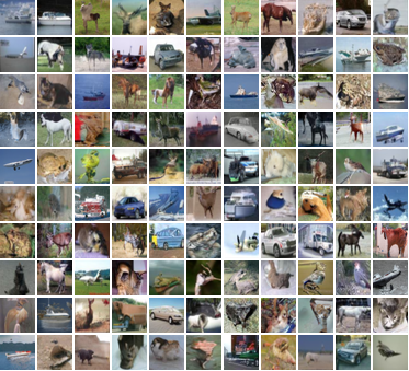
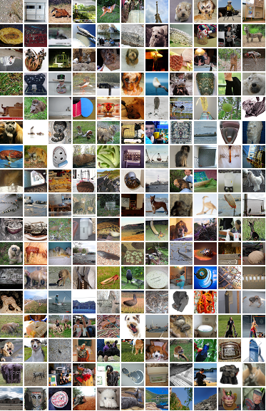
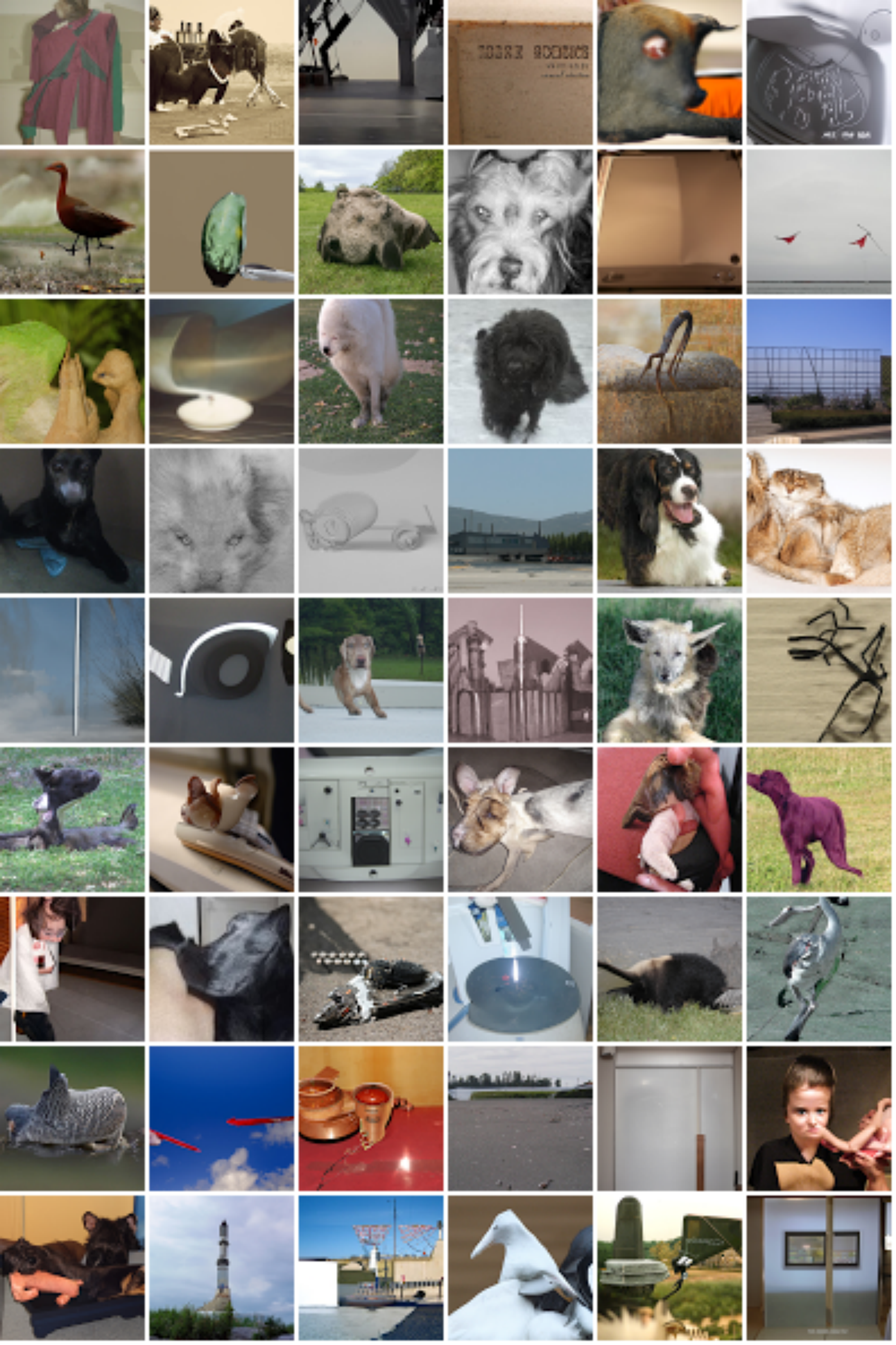
N Lossless compression

Section Summary: The section explains how a diffusion model can be adapted into a lossless data compression technique using a method called bits-back coding, which efficiently encodes both the data and hidden variables by borrowing random bits and relating the compression efficiency to a key model metric known as the negative VLB. As a demonstration, the authors tested this on the CIFAR10 image dataset, achieving compression rates close to theoretical limits for shorter processing steps, but with some gaps for longer ones due to challenges in handling tiny probabilities and the high computational demands. They improved practical performance by discretizing continuous elements and encrypting data streams, suggesting further refinements for scaling to more steps as an area for future exploration.

For a fixed number of evaluation timesteps $T_{eval}$, our diffusion model in discrete time is a hierarchical latent variable model that can be turned into a lossless compression algorithm using bits-back coding ([33]). Assuming a source of auxiliary random bits is available alongside the data, bits-back coding encodes a latent and data together, with the latent sampled from the approximate posterior using the auxiliary random bits. The net coding cost of bits-back coding is given by subtracting the number of bits needed to sample the latent from the number of bits needed to encode the latent and data using the reverse process, so the negative VLB of our discrete time model is the theoretical expected coding cost for bits-back coding.

As a proof of concept for lossless compression using our model, Table 2 reports net codelengths on the CIFAR10 test set for various settings of $T_{eval}$ using BB-ANS ([34]), a practical implementation of bits-back coding based on asymmetric numeral systems ([35]). Since diffusion models have Markov forward and reverse processes, we use the Bit-Swap implementation of BB-ANS [41]. Practical implementations of bits-back coding must discretize continuous latent variables and their associated continuous probability distributions; for simplicity, our implementation uses a uniform discretization of the continuous latents and their associated Gaussian conditionals from the forward and reverse processes. Additionally, we found it crucial to encrypt the ANS bitstream before each decoding operation to ensure clean bits for sampling from the approximate posterior; we did so by applying the XOR operation to the ANS bitstream with pseudorandom bits from a fixed sequence of seeds. For example, without cleaning the bitstream using encryption, compressing a batch of 100 examples using $T_{eval}=250$ costs 2.74 bits per byte, but with encryption, the cost improves to 2.68 bits per dimension.

For a small number of timesteps $T_{eval}$, our bits-back implementation attains net codelengths that agree closely with the negative VLB, but there is some discrepancy for large $T_{eval}$. This is due to inaccuracies in the compression algorithm to represent discretized Gaussians with small standard deviations, and small discrepancies in codelength compound into a gap of up to 0.05 bits per dimension when $T$ is large. (In prior work, e.g. [41, 42, 43], practical implementations of bits-back coding have been tested on latent variable models with only tens of layers, not hundreds.) In addition, a large number of timesteps makes compression computationally expensive, because a neural network forward pass must be run for each timestep. Closing the codelength gap with an efficient implementation of bits-back coding for a large number of timesteps is an interesting avenue for future work.

O Density estimation on additional data sets

Section Summary: In response to a reviewer, the researchers tested their image density estimation model on two new datasets featuring higher-resolution but less varied images, achieving a test set likelihood of 2.14 bits per dimension on CelebA-HQ and 1.44 on LSUN bedrooms, both at 128 by 128 pixels. These datasets lack standard benchmarks for comparison, so the results simply offer a rough idea of how well the method performs with sharper images. The model builds on their earlier version for 64 by 64 pixel images by adding a layer of 16 processing steps with 128 channels to handle the higher resolution, including a downsampling technique similar to prior work.

At the request of one of the reviewers we also ran our model on additional data sets of higher resolution, less diverse, images. Specifically, we obtain a test set likelihood of $2.14$ bits per dim on CelebA-HQ ([44]), and $1.44$ on LSUN bedrooms [45], both at $128 \times 128$ resolution. Since these are not established benchmarks in density estimation, and since downsampling methods in the literature are not consistent, we don't compare against previous methods for these data sets. Our results are provided purely to give a ballpark estimate of how well our proposed method scales to higher resolution images.

The model used for these data sets is based on that used for Imagenet $64 \times 64$, with an additional level in the UNet at resolution $128 \times 128$, consisting of 16 residual layers using 128 channels. Our model downsamples between the $128 \times 128$ and $64 \times 64$ resolutions, similar to e.g. Ho et al. [4], but unlike the models we used for the other data sets we considered.

References

Section Summary: This references section lists numerous academic papers and books that form the foundational works in machine learning, focusing on generative models for creating audio, images, and other data. It includes influential studies on techniques like WaveNet for raw audio generation, sequence-to-sequence learning with neural networks, and diffusion probabilistic models that help computers learn and reproduce complex patterns from data. Key contributors such as Ilya Sutskever, Diederik P. Kingma, and Geoffrey Hinton are cited, covering developments from 2003 to 2021, with the list ending abruptly on a work about neural networks.

[1] Aaron van den Oord, Sander Dieleman, Heiga Zen, Karen Simonyan, Oriol Vinyals, Alex Graves, Nal Kalchbrenner, Andrew Senior, and Koray Kavukcuoglu. Wavenet: A generative model for raw audio. arXiv preprint arXiv:1609.03499, 2016.

[2] Ilya Sutskever, Oriol Vinyals, and Quoc V Le. Sequence to sequence learning with neural networks. arXiv preprint arXiv:1409.3215, 2014.

[3] David JC MacKay. Information theory, inference and learning algorithms. Cambridge university press, 2003.

[4] Jonathan Ho, Ajay Jain, and Pieter Abbeel. Denoising diffusion probabilistic models. arXiv preprint arXiv:2006.11239, 2020.

[5] Yang Song, Jascha Sohl-Dickstein, Diederik P Kingma, Abhishek Kumar, Stefano Ermon, and Ben Poole. Score-Based Generative Modeling Through Stochastic Differential Equations. In International Conference on Learning Representations, 2021b.

[6] Alex Nichol and Prafulla Dhariwal. Improved denoising diffusion probabilistic models. arXiv preprint arXiv:2102.09672, 2021.

[7] Zhifeng Kong, Wei Ping, Jiaji Huang, Kexin Zhao, and Bryan Catanzaro. Diffwave: A versatile diffusion model for audio synthesis. arXiv preprint arXiv:2009.09761, 2020.

[8] Nanxin Chen, Yu Zhang, Heiga Zen, Ron J. Weiss, Mohammad Norouzi, and William Chan. Wavegrad: Estimating gradients for waveform generation. arXiv preprint arXiv:2009.00713, 2020.

[9] Jascha Sohl-Dickstein, Eric Weiss, Niru Maheswaranathan, and Surya Ganguli. Deep unsupervised learning using nonequilibrium thermodynamics. In International Conference on Machine Learning, pages 2256–2265, 2015.

[10] Diederik P Kingma and Max Welling. Auto-encoding variational Bayes. International Conference on Learning Representations, 2013.

[11] Danilo J Rezende, Shakir Mohamed, and Daan Wierstra. Stochastic backpropagation and approximate inference in deep generative models. In International Conference on Machine Learning, pages 1278–1286, 2014.

[12] Yang Song and Stefano Ermon. Improved techniques for training score-based generative models. In Hugo Larochelle, Marc'Aurelio Ranzato, Raia Hadsell, Maria-Florina Balcan, and Hsuan-Tien Lin, editors, Advances in Neural Information Processing Systems 33: Annual Conference on Neural Information Processing Systems 2020, NeurIPS 2020, December 6-12, 2020, virtual, 2020.

[13] Ruiqi Gao, Yang Song, Ben Poole, Ying Nian Wu, and Diederik P Kingma. Learning energy-based models by diffusion recovery likelihood. arXiv preprint arXiv:2012.08125, 2020.

[14] Yang Song and Stefano Ermon. Generative modeling by estimating gradients of the data distribution. In Advances in Neural Information Processing Systems, pages 11895–11907, 2019.

[15] Yang Song, Conor Durkan, Iain Murray, and Stefano Ermon. Maximum likelihood training of score-based diffusion models. arXiv e-prints, pages arXiv–2101, 2021a.

[16] Chin-Wei Huang, Jae Hyun Lim, and Aaron Courville. A variational perspective on diffusion-based generative models and score matching. arXiv preprint arXiv:2106.02808, 2021.

[17] Arash Vahdat, Karsten Kreis, and Jan Kautz. Score-based generative modeling in latent space. arXiv preprint arXiv:2106.05931, 2021.

[18] Diederik P Kingma, Tim Salimans, Rafal Jozefowicz, Xi Chen, Ilya Sutskever, and Max Welling. Improved variational inference with inverse autoregressive flow. In Advances in Neural Information Processing Systems, pages 4743–4751, 2016.

[19] Rewon Child. Very deep VAEs generalize autoregressive models and can outperform them on images. arXiv preprint arXiv:2011.10650, 2020.

[20] Arash Vahdat and Jan Kautz. Nvae: A deep hierarchical variational autoencoder. arXiv preprint arXiv:2007.03898, 2020.

[21] Diederik P Kingma and Prafulla Dhariwal. Glow: Generative flow with invertible 1x1 convolutions. arXiv preprint arXiv:1807.03039, 2018.

[22] Jonathan Ho, Xi Chen, Aravind Srinivas, Yan Duan, and Pieter Abbeel. Flow++: Improving flow-based generative models with variational dequantization and architecture design. In International Conference on Machine Learning, pages 2722–2730. PMLR, 2019a.

[23] Aaron Van Oord, Nal Kalchbrenner, and Koray Kavukcuoglu. Pixel recurrent neural networks. In International Conference on Machine Learning, pages 1747–1756, 2016.

[24] Tim Salimans, Andrej Karpathy, Xi Chen, and Diederik P Kingma. Pixelcnn++: Improving the pixelcnn with discretized logistic mixture likelihood and other modifications. arXiv preprint arXiv:1701.05517, 2017.

[25] Niki Parmar, Ashish Vaswani, Jakob Uszkoreit, Lukasz Kaiser, Noam Shazeer, Alexander Ku, and Dustin Tran. Image transformer. In International Conference on Machine Learning, pages 4055–4064. PMLR, 2018.

[26] Jacob Menick and Nal Kalchbrenner. Generating high fidelity images with subscale pixel networks and multidimensional upscaling. arXiv preprint arXiv:1812.01608, 2018.

[27] Rewon Child, Scott Gray, Alec Radford, and Ilya Sutskever. Generating long sequences with sparse transformers. arXiv preprint arXiv:1904.10509, 2019.

[28] Aurko Roy, Mohammad Saffar, Ashish Vaswani, and David Grangier. Efficient content-based sparse attention with routing transformers. Transactions of the Association for Computational Linguistics, 9:53–68, 2021.

[29] Heewoo Jun, Rewon Child, Mark Chen, John Schulman, Aditya Ramesh, Alec Radford, and Ilya Sutskever. Distribution augmentation for generative modeling. In International Conference on Machine Learning, pages 5006–5019. PMLR, 2020.

[30] Samarth Sinha and Adji B Dieng. Consistency regularization for variational auto-encoders. arXiv preprint arXiv:2105.14859, 2021.

[31] Alex Krizhevsky, Geoffrey Hinton, et al. Learning multiple layers of features from tiny images. 2009.

[32] Jia Deng, Wei Dong, Richard Socher, Li-Jia Li, Kai Li, and Li Fei-Fei. Imagenet: A large-scale hierarchical image database. In 2009 IEEE conference on computer vision and pattern recognition, pages 248–255. Ieee, 2009.

[33] Geoffrey E Hinton and Drew Van Camp. Keeping the neural networks simple by minimizing the description length of the weights. In Proceedings of the Sixth Annual Conference on Computational Learning Theory, pages 5–13, 1993.

[34] James Townsend, Thomas Bird, and David Barber. Practical lossless compression with latent variables using bits back coding. In International Conference on Learning Representations, 2018.

[35] Jarek Duda. Asymmetric numeral systems. arXiv preprint arXiv:0902.0271, 2009.

[36] Olaf Ronneberger, Philipp Fischer, and Thomas Brox. U-net: Convolutional networks for biomedical image segmentation. In International Conference on Medical image computing and computer-assisted intervention, pages 234–241. Springer, 2015.

[37] Ilya Loshchilov and Frank Hutter. Decoupled weight decay regularization. arXiv preprint arXiv:1711.05101, 2017.

[38] Matthew Tancik, Pratul P Srinivasan, Ben Mildenhall, Sara Fridovich-Keil, Nithin Raghavan, Utkarsh Singhal, Ravi Ramamoorthi, Jonathan T Barron, and Ren Ng. Fourier features let networks learn high frequency functions in low dimensional domains. arXiv preprint arXiv:2006.10739, 2020.

[39] Jiaming Song, Chenlin Meng, and Stefano Ermon. Denoising diffusion implicit models. arXiv preprint arXiv:2010.02502, 2020.

[40] Pascal Vincent. A connection between score matching and denoising autoencoders. Neural computation, 23(7):1661–1674, 2011.

[41] Friso Kingma, Pieter Abbeel, and Jonathan Ho. Bit-swap: Recursive bits-back coding for lossless compression with hierarchical latent variables. In International Conference on Machine Learning, pages 3408–3417. PMLR, 2019.

[42] Jonathan Ho, Evan Lohn, and Pieter Abbeel. Compression with flows via local bits-back coding. In Advances in Neural Information Processing Systems, pages 3874–3883, 2019b.

[43] James Townsend, Thomas Bird, Julius Kunze, and David Barber. HiLLoC: lossless image compression with hierarchical latent variable models. In International Conference on Learning Representations, 2020.

[44] Tero Karras, Timo Aila, Samuli Laine, and Jaakko Lehtinen. Progressive growing of gans for improved quality, stability, and variation. arXiv preprint arXiv:1710.10196, 2017.

[45] Fisher Yu, Ari Seff, Yinda Zhang, Shuran Song, Thomas Funkhouser, and Jianxiong Xiao. Lsun: Construction of a large-scale image dataset using deep learning with humans in the loop. arXiv preprint arXiv:1506.03365, 2015.