Stochastic Backpropagation and Approximate Inference in Deep Generative Models

Danilo J. Rezende, Shakir Mohamed, Daan Wierstra {danilor, shakir, daanw}@google.com Google DeepMind, London

Abstract

We marry ideas from deep neural networks and approximate Bayesian inference to derive a generalised class of deep, directed generative models, endowed with a new algorithm for scalable inference and learning. Our algorithm introduces a recognition model to represent an approximate posterior distribution and uses this for optimisation of a variational lower bound. We develop stochastic backpropagation – rules for gradient backpropagation through stochastic variables – and derive an algorithm that allows for joint optimisation of the parameters of both the generative and recognition models. We demonstrate on several real-world data sets that by using stochastic backpropagation and variational inference, we obtain models that are able to generate realistic samples of data, allow for accurate imputations of missing data, and provide a useful tool for high-dimensional data visualisation.

Executive Summary: In the rapidly evolving field of machine learning, there is a growing need for probabilistic models that can handle complex, high-dimensional data while enabling tasks like prediction, filling in missing information, estimating uncertainty, and generating synthetic samples. These capabilities are crucial for applications in science, such as simulating genetic processes or robotic behaviors, where traditional models often struggle with scalability and accuracy. Current directed generative models, which build data hierarchically from simple distributions, excel at sampling but face challenges in performing efficient inference—essentially, figuring out the hidden factors behind observed data. This gap limits their use in real-world scenarios demanding fast, reliable probabilistic reasoning.

This paper sets out to address that by introducing a new class of deep generative models called deep latent Gaussian models (DLGMs), which use layered Gaussian distributions to capture intricate data structures. The authors aimed to develop an algorithm for scalable inference and learning that jointly optimizes both the model's data-generating process and an auxiliary "recognition" component for approximating hidden states.

The approach combines ideas from deep neural networks—layers of interconnected nodes that learn patterns—with approximate Bayesian inference, a statistical method to handle uncertainty. They created a generative model that starts with simple noise and applies non-linear transformations across multiple layers to produce data, such as images. To make inference tractable, they introduced a recognition model, essentially a neural network that encodes observed data into Gaussian approximations of the hidden variables. The key innovation is stochastic backpropagation, a technique for computing gradients (directions for model improvement) through random variables, allowing optimization of a variational lower bound on data likelihood. This uses Monte Carlo sampling for estimates and draws from real-world datasets like handwritten digits (MNIST), natural images (CIFAR-10), and faces (Frey), with sample sizes in the thousands to tens of thousands, over training periods of several hours on standard hardware. Assumptions include Gaussian priors for latents and neural network flexibility for transformations, ensuring computational efficiency without full exact computations.

The most important results show that DLGMs outperform or match leading models on key metrics. First, they achieve high data likelihoods, with negative log-probability scores of 86.60 on binarized MNIST—about 5-10% better than non-linear Gaussian belief networks and competitive with advanced autoregressive models like NADE. Second, the models generate realistic samples, producing clear handwritten digits, toy objects, and face patches that closely resemble training data. Third, they excel at imputing missing data, accurately reconstructing images even when 60-80% of pixels are absent or a central region is removed, as demonstrated on street view numbers and faces. Fourth, for visualization, projecting high-dimensional data to 2D latent spaces separates categories like digit classes into distinct clusters, revealing underlying structures. Finally, the recognition model provides efficient posterior approximations, concentrating samples where true uncertainty lies, unlike prior-based methods that waste effort on irrelevant areas.

These findings mean DLGMs offer a practical tool for generative tasks, reducing costs in simulation by producing diverse, high-fidelity samples without exhaustive computation. They lower risks in prediction by quantifying uncertainty better than deterministic neural networks, enhance safety in applications like robotics through reliable imputation, and speed up analysis timelines for high-dimensional data in policy or compliance contexts, such as image forensics. Surprisingly, the method surpasses expectations from older variational techniques like wake-sleep, which often converge slowly, by enabling joint optimization that tightens the approximation gap—potentially halving inference time compared to iterative alternatives.

Leaders should prioritize integrating DLGMs into pipelines for data generation and analysis, starting with pilots on image or sequential datasets to replace less scalable models. Key options include using diagonal covariances for faster training (at slight accuracy cost) versus structured ones for better posterior capture; trade-offs involve compute time versus fidelity. Further work is needed, such as testing on larger-scale data (e.g., video) or incorporating convolutional layers for spatial data, before full deployment in production systems.

While robust on tested benchmarks, limitations include reliance on Gaussian approximations, which may underfit non-elliptical posteriors, and quadratic complexity per layer that scales with latent dimensions, potentially straining very deep models. Data gaps exist for non-image domains like text or time series. Overall confidence is high for generative and imputation tasks on structured data, but caution is advised for extrapolation to unseen distributions without additional validation.

1. Introduction

Section Summary: Researchers in machine learning and statistics are working hard to build reliable probabilistic models that can handle tasks like predicting outcomes, filling in missing data, estimating uncertainties, and generating simulations for fields such as genetics and robotics. These models need to be deep to capture complex patterns, quick at producing samples, and efficient for large datasets, but existing ones often struggle with accurate inferences. This introduction proposes a new type of deep generative model using Gaussian hidden variables, paired with a recognition system for approximate inference, which allows joint training of both parts through adapted neural network techniques, and highlights contributions in model design, scalable inference, and practical evaluations for tasks like simulation and prediction.

There is an immense effort in machine learning and statistics to develop accurate and scalable probabilistic models of data. Such models are called upon whenever we are faced with tasks requiring probabilistic reasoning, such as prediction, missing data imputation and uncertainty estimation; or in simulation-based analyses, common in many scientific fields such as genetics, robotics and control that require generating a large number of independent samples from the model.

Recent efforts to develop generative models have focused on directed models, since samples are easily obtained by ancestral sampling from the generative process. Directed models such as belief networks and similar latent variable models ([1, 2, 3, 4, 5, 6]) can be easily sampled from, but in most cases, efficient inference algorithms have remained elusive. These efforts, combined with the demand for accurate probabilistic inferences and fast simulation, lead us to seek generative models that are i) deep, since hierarchical architectures allow us to capture complex structure in the data, ii) allow for fast sampling of fantasy data from the inferred model, and iii) are computationally tractable and scalable to high-dimensional data.

We meet these desiderata by introducing a class of deep, directed generative models with Gaussian latent variables at each layer. To allow for efficient and tractable inference, we use introduce an approximate representation of the posterior over the latent variables using a recognition model that acts as a stochastic encoder of the data. For the generative model, we derive the objective function for optimisation using variational principles; for the recognition model, we specify its structure and regularisation by exploiting recent advances in deep learning. Using this construction, we can train the entire model by a modified form of gradient backpropagation that allows for optimisation of the parameters of both the generative and recognition models jointly.

We build upon the large body of prior work (in Section 6) and make the following contributions:

• We combine ideas from deep neural networks and probabilistic latent variable modelling to derive a general class of deep, non-linear latent Gaussian models (Section 2).
• We present a new approach for scalable variational inference that allows for joint optimisation of both variational and model parameters by exploiting the properties of latent Gaussian distributions and gradient backpropagation (Section 3 and Section 4).
• We provide a comprehensive and systematic evaluation of the model demonstrating its applicability to problems in simulation, visualisation, prediction and missing data imputation (Section 5).

2. Deep Latent Gaussian Models

Section Summary: Deep latent Gaussian models are a type of hierarchical machine learning framework where hidden variables follow Gaussian distributions across multiple layers, allowing the generation of data by starting with random noise at the top layer and applying nonlinear transformations and more noise as it moves downward to produce observable outputs. This setup transforms a simple spherical Gaussian distribution into complex patterns that match real-world data, generalizing simpler models like factor analysis or nonlinear belief networks. The models use probabilistic equations to define this process and rely on advanced inference techniques to learn from data, with the section proposing a new, scalable approach to improve efficiency.

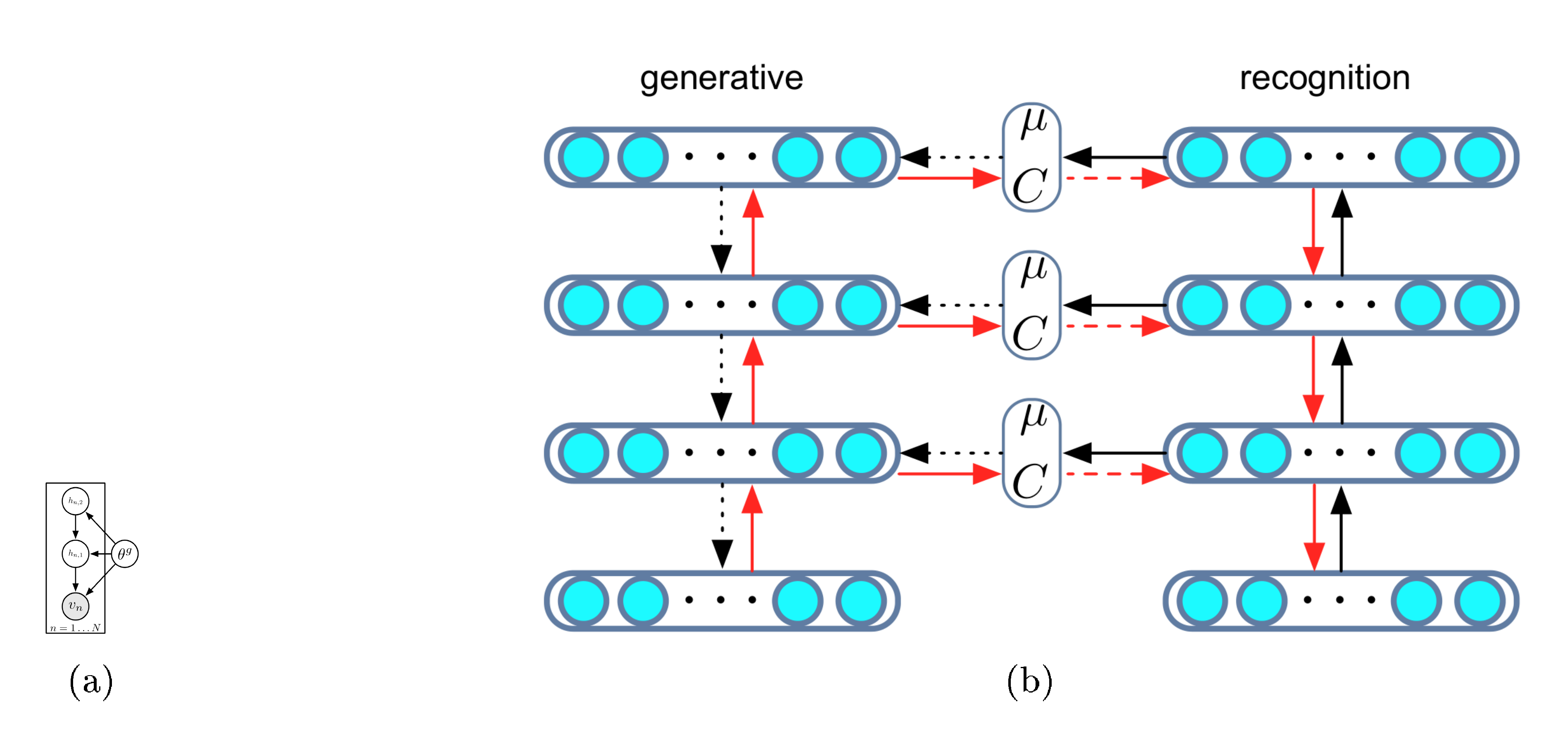
Deep latent Gaussian models (DLGMs) are a general class of deep directed graphical models that consist of Gaussian latent variables at each layer of a processing hierarchy. The model consists of $L$ layers of latent variables. To generate a sample from the model, we begin at the top-most layer ($L$) by drawing from a Gaussian distribution. The activation $\mathbf{h}{l}$ at any lower layer is formed by a non-linear transformation of the layer above $\mathbf{h}{l+1}$, perturbed by Gaussian noise. We descend through the hierarchy and generate observations $\mathbf{v}$ by sampling from the observation likelihood using the activation of the lowest layer $\mathbf{h}_1$. This process is described graphically in Figure 1a.

This generative process is described as follows:

$ \begin{align} \boldsymbol{\xi}l & \sim \mathcal{N}(\boldsymbol{\xi}l | \boldsymbol{0}, \mathbf{I}), \quad l = 1, \ldots, L \ \mathbf{h}{L} &= \mathbf{G}{L} \boldsymbol{\xi}{L}, \tag{a} \ \mathbf{h}{l} &= T_l(\mathbf{h}{l+1}) + \mathbf{G}{l} \boldsymbol{\xi}{l}, \quad l =1 \ldots L-1 \tag{b} \ \mathbf{v} & \sim \pi(\mathbf{v} | T_0(\mathbf{h}{1})), \tag{c} \end{align}\tag{1} $

where $\boldsymbol{\xi}_l$ are mutually independent Gaussian variables. The transformations $T_l$ represent multi-layer perceptrons (MLPs) and $\mathbf{G}_l$ are matrices. At the visible layer, the data is generated from any appropriate distribution $\pi(\mathbf{v} | \cdot)$ whose parameters are specified by a transformation of the first latent layer. Throughout the paper we refer to the set of parameters in this generative model by $\boldsymbol{\theta}^g$, i.e. the parameters of the maps $T_l$ and the matrices $G_l$. This construction allows us to make use of as many deterministic and stochastic layers as needed. We adopt a weak Gaussian prior over $\boldsymbol{\theta}^g$, $p(\boldsymbol{\theta}^g) = \mathcal{N}(\boldsymbol{\theta}| \boldsymbol{0}, \kappa \mathbf{I})$.

The joint probability distribution of this model can be expressed in two equivalent ways:

$ \begin{align} & p(\mathbf{v}, ! \mathbf{h})! =! p(! \mathbf{v}| \mathbf{h}_1, ! \boldsymbol{\theta}^g) p(\mathbf{h}L | \boldsymbol{\theta}^g) p(! \boldsymbol{\theta}^g!) !!\prod{l=1}^{L

• 1}!! p_l(\mathbf{h}l | \mathbf{h}{l!+!1}, ! \boldsymbol{\theta}^g)\tag{a} \ & p(\mathbf{v}, ! \boldsymbol{\xi})! = p(\mathbf{v}| \mathbf{h}1(\boldsymbol{\xi}{1 \ldots L}), \boldsymbol{\theta}^g) p(\boldsymbol{\theta}^g) \prod_{l=1}^{L} \mathcal{N}(\boldsymbol{\xi}| \boldsymbol{0}, \mathbf{I}). \tag{b} \end{align}\tag{2} $

The conditional distributions $p(\mathbf{h}l | \mathbf{h}{l+1})$ are implicitly defined by equation 1ab and are Gaussian distributions with mean $\boldsymbol{\mu}l = T_l(\mathbf{h}{l+1})$ and covariance $\mathbf{S}_l = \mathbf{G}_l \mathbf{G}l^\top$. Equation 2ab makes explicit that this generative model works by applying a complex non-linear transformation to a spherical Gaussian distribution $p(\boldsymbol{\xi}) = \prod{l=1}^{L} \mathcal{N}(\boldsymbol{\xi}_l| \boldsymbol{0}, \mathbf{I})$ such that the transformed distribution tries to match the empirical distribution. A graphical model corresponding to equation 2aa is shown in Figure 1(a).

This specification for deep latent Gaussian models (DLGMs) generalises a number of well known models. When we have only one layer of latent variables and use a linear mapping $T(\cdot)$, we recover factor analysis ([4]) – more general mappings allow for a non-linear factor analysis ([7]). When the mappings are of the form $T_l(\mathbf{h}) = \mathbf{A}_l f(\mathbf{h}) + \mathbf{b}_l$, for simple element-wise non-linearities $f$ such as the probit function or the rectified linearity, we recover the non-linear Gaussian belief network ([8]). We describe the relationship to other existing models in Section 6. Given this specification, our key task is to develop a method for tractable inference. A number of approaches are known and widely used, and include: mean-field variational EM ([9]); the wake-sleep algorithm ([10]); and stochastic variational methods and related control-variate estimators ([11, 12, 13]). We also follow a stochastic variational approach, but shall develop an alternative to these existing inference algorithms that overcomes many of their limitations and that is both scalable and efficient.

3. Stochastic Backpropagation

Section Summary: Stochastic backpropagation is a technique for efficiently computing gradients in machine learning models with hidden variables, where the challenge lies in calculating expectations over distributions that depend on the model's parameters. For Gaussian distributions, it uses special mathematical identities to estimate these gradients by sampling from the distribution and applying rules that account for changes in the mean and covariance, avoiding direct and costly computations. This approach extends to other distributions through methods like integral rules or transforming variables from a simpler base distribution, enabling practical approximations with low computational cost.

Gradient descent methods in latent variable models typically require computations of the form $\nabla_\theta \mathbb{E}{q\theta}\left[f(\boldsymbol{\xi})\right]$, where the expectation is taken with respect to a distribution $q_\theta(\cdot)$ with parameters $\boldsymbol{\theta}$, and $f$ is a loss function that we assume to be integrable and smooth. This quantity is difficult to compute directly since i) the expectation is unknown for most problems, and ii) there is an indirect dependency on the parameters of $q$ over which the expectation is taken.

We now develop the key identities that are used to allow for efficient inference by exploiting specific properties of the problem of computing gradients through random variables. We refer to this computational strategy as stochastic backpropagation.

3.1 Gaussian Backpropagation (GBP)

When the distribution $q$ is a $K$-dimensional Gaussian $\mathcal{N}(\boldsymbol{\xi} | \boldsymbol{\mu}, \mathbf{C})$ the required gradients can be computed using the Gaussian gradient identities:

$ \begin{align} \nabla_{\mu_i} \mathbb{E}{ \tiny{\mathcal{N}(\boldsymbol{\mu}, \mathbf{C})} } \left[f(\boldsymbol{\xi}) \right] &= \mathbb{E}{ \tiny{\mathcal{N}(\boldsymbol{\mu}, \mathbf{C})} } \left[\nabla_{\xi_i} f(\boldsymbol{\xi}) \right], \tag{a} \ \nabla_{C_{ij}} \mathbb{E}{ \tiny{\mathcal{N}(\boldsymbol{\mu}, \mathbf{C}) } }\left [f(\boldsymbol{\xi}) \right] &= \tfrac{1}{2} \mathbb{E}{ \tiny{\mathcal{N}(\boldsymbol{\mu}, \mathbf{C})} } \left [\nabla^2_{\xi_i, \xi_j} f(\boldsymbol{\xi}) \right], \tag{b} \end{align}\tag{3} $

which are due to the theorems by [14] and [15], respectively. These equations are true in expectation for any integrable and smooth function $f(\boldsymbol{\xi})$. Equation 3aa is a direct consequence of the location-scale transformation for the Gaussian (discussed in Section 3.2). Equation 3ab can be derived by successive application of the product rule for integrals; we provide the proofs for these identities in Appendix B.

Equations 3aa and 3ab are especially interesting since they allow for unbiased gradient estimates by using a small number of samples from $q$. Assume that both the mean $\boldsymbol{\mu}$ and covariance matrix $\mathbf{C}$ depend on a parameter vector $\boldsymbol{\theta}$. We are now able to write a general rule for Gaussian gradient computation by combining equations 3aa and 3ab and using the chain rule:

$ !!!\nabla_{!\tiny{\boldsymbol{\theta}}}\mathbb{E}{! \tiny{\mathcal{N}!\left(\boldsymbol{\mu}, \mathbf{C}\right)} }! \left [f(\boldsymbol{\xi}) \right] !=! \mathbb{E}{! \tiny{\mathcal{N}!\left(\boldsymbol{\mu}, \mathbf{C}\right)} } !!\left [! \mathbf{g}!^\top! \frac{\partial \boldsymbol{\mu}}{\partial \boldsymbol{\theta}}! +! \tfrac{1}{2}! \operatorname{Tr}! \left(!\mathbf{H} \frac{\partial \mathbf{C}}{\partial \boldsymbol{\theta}} !\right) !\right]\tag{4} $

where $\mathbf{g}$ and $\mathbf{H}$ are the gradient and the Hessian of the function $f(\boldsymbol{\xi})$, respectively. Equation 4 can be interpreted as a modified backpropagation rule for Gaussian distributions that takes into account the gradients through the mean $\boldsymbol{\mu}$ and covariance $\mathbf{C}$. This reduces to the standard backpropagation rule when $\mathbf{C}$ is constant. Unfortunately this rule requires knowledge of the Hessian matrix of $f(\boldsymbol{\xi})$, which has an algorithmic complexity $O(K^3)$. For inference in DLGMs, we later introduce an unbiased though higher variance estimator that requires only quadratic complexity.

3.2 Generalised Backpropagation Rules

We describe two approaches to derive general backpropagation rules for non-Gaussian $q$-distributions.

Using the product rule for integrals. For many exponential family distributions, it is possible to find a function $B(\boldsymbol{\xi}; \boldsymbol{\theta})$ to ensure that

$ \begin{align} \nabla_{\tiny{\boldsymbol{\theta}}} \mathbb{E}{\tiny{p(\boldsymbol{\xi} | \boldsymbol{\theta})}} [f(\boldsymbol{\xi})] !=!! = - \mathbb{E}{\tiny{p (\boldsymbol{\xi} | \boldsymbol{\theta})}} [\nabla_{\tiny{\boldsymbol{\xi}}} [B (\boldsymbol{\xi}; \boldsymbol{\theta}) f (\boldsymbol{\xi})]]. \nonumber \end{align} $

That is, we express the gradient with respect to the parameters of $q$ as an expectation of gradients with respect to the random variables themselves. This approach can be used to derive rules for many distributions such as the Gaussian, inverse Gamma and log-Normal. We discuss this in more detail in Appendix C.

Using suitable co-ordinate transformations.

We can also derive stochastic backpropagation rules for any distribution that can be written as a smooth, invertible transformation of a standard base distribution. For example, any Gaussian distribution $\mathcal{N}(\boldsymbol{\mu}, \mathbf{C})$ can be obtained as a transformation of a spherical Gaussian $\boldsymbol{\epsilon} \sim \mathcal{N}(\boldsymbol{0}, \mathbf{I})$, using the transformation $y = \boldsymbol{\mu} + \mathbf{R} \boldsymbol{\epsilon}$ and $\mathbf{C} = \mathbf{R} \mathbf{R}!^\top!!$. The gradient of the expectation with respect to $\mathbf{R}$ is then:

$ \begin{align} \nabla_{\tiny{\mathbf{R}}} \mathbb{E}{! \mathcal{N}!\left(\tiny{\boldsymbol{\mu}, \mathbf{C}}\right) } \left[f(\boldsymbol{\xi}) \right] &=\nabla{\tiny{\mathbf{R}}} \mathbb{E}{\tiny{\mathcal{N}(0, I)} } \left [f(\small{\boldsymbol{\mu} + \mathbf{R} \boldsymbol{\epsilon}}) \right] \nonumber \ &= \mathbb{E}{ \tiny{\mathcal{N}(0, I)} } \left [\boldsymbol{\epsilon} \mathbf{g}^\top \right], \end{align}\tag{5} $

where $\mathbf{g}$ is the gradient of $f$ evaluated at $\boldsymbol{\mu} + \mathbf{R} \boldsymbol{\epsilon}$ and provides a lower-cost alternative to Price's theorem Equation 3ab. Such transformations are well known for many distributions, especially those with a self-similarity property or location-scale formulation, such as the Gaussian, Student's $t$-distribution, stable distributions, and generalised extreme value distributions.

Stochastic backpropagation in other contexts. The Gaussian gradient identities described above do not appear to be widely used. These identities have been recognised by [16] for variational inference in Gaussian process regression, and following this work, by [17] for parameter learning in large neural networks. Concurrently with this paper, [18] present an alternative discussion of stochastic backpropagation. Our approaches were developed simultaneously and provide complementary perspectives on the use and derivation of stochastic backpropagation rules.

4. Scalable Inference in DLGMs

Section Summary: To perform inference in deep latent Gaussian models, researchers approximate the difficult task of integrating over hidden variables by optimizing a lower bound called the free energy, which balances a measure of how well an assumed distribution matches the true probabilities against the model's ability to reconstruct the observed data. This assumed distribution, known as the recognition model, is a flexible Gaussian setup powered by neural networks that conditions on the input data, enabling fast and shared computations across examples for quicker training and testing. The approach relies on analytical shortcuts for key calculations, added noise for stability, and gradient-based optimization using random sampling to make the whole process scalable.

We use the matrix $\mathbf{V}$ to refer to the full data set of size $N\times D$ with observations $\mathbf{v}n = [v{n1}, \ldots, v_{nD}]^\top$.

4.1 Free Energy Objective

To perform inference in DLGMs we must integrate out the effect of any latent variables – this requires us to compute the integrated or marginal likelihood. In general, this will be an intractable integration and instead we optimise a lower bound on the marginal likelihood. We introduce an approximate posterior distribution $q(\cdot)$ and apply Jensen's inequality following the variational principle ([9]) to obtain:

$ \begin{align} \mathcal{L}(\mathbf{V}) &= -\log p(\mathbf{V}) = -\log \int p(\mathbf{V} | \boldsymbol{\xi}, \boldsymbol{\theta}^g) p(\boldsymbol{\xi}, \boldsymbol{\theta}^g) d \boldsymbol{\xi} \nonumber \ & = -\log \int \frac{ q(\boldsymbol{\xi})}{q(\boldsymbol{\xi}) } p(\mathbf{V} | \boldsymbol{\xi}, \boldsymbol{\theta}^g) p(\boldsymbol{\xi}, \boldsymbol{\theta}^g) d \boldsymbol{\xi} \ {\leq} \mathcal{F}(\mathbf{V}) & !=!D_{KL}[q(\boldsymbol{\xi}) | p(\boldsymbol{\xi})]! -! \mathbb{E}_{q}\left[\log p(\mathbf{V} | \boldsymbol{\xi}, ! \boldsymbol{\theta}^g)p(\boldsymbol{\theta}^g)\right] .\nonumber \end{align}\tag{6} $

This objective consists of two terms: the first is the KL-divergence between the variational distribution and the prior distribution (which acts a regulariser), and the second is a reconstruction error.

We specify the approximate posterior as a distribution $q(\boldsymbol{\xi} | \mathbf{v})$ that is conditioned on the observed data. This distribution can be specified as any directed acyclic graph where each node of the graph is a Gaussian conditioned, through linear or non-linear transformations, on its parents. The joint distribution in this case is non-Gaussian, but stochastic backpropagation can still be applied.

For simplicity, we use a $q(\boldsymbol{\xi} | \mathbf{v})$ that is a Gaussian distribution that factorises across the $L$ layers (but not necessarily within a layer):

$ q(\boldsymbol{\xi} | \mathbf{V}, \boldsymbol{\theta}^r) = \prod_{n=1}^N \prod_{l=1}^L \mathcal{N}\left(\boldsymbol{\xi}{n, l} | \boldsymbol{\mu}{l}(\mathbf{v}_n), \mathbf{C}_l(\mathbf{v}_n) \right),\tag{7} $

where the mean $\boldsymbol{\mu}_l(\cdot)$ and covariance $\mathbf{C}_l(\cdot)$ are generic maps represented by deep neural networks. Parameters of the $q$-distribution are denoted by the vector $\boldsymbol{\theta}^r$.

For a Gaussian prior and a Gaussian recognition model, the KL term in Equation 6 can be computed analytically and the free energy becomes:

$ \begin{align} D_{!KL}&[\mathcal{N}(\boldsymbol{\mu}, ! \mathbf{C})| \mathcal{N}(\boldsymbol{0}, ! \mathbf{I})] !=! \tfrac{1}{2}! \left[\textrm{Tr}(! \mathbf{C}!)!-!\log| \mathbf{C}| !+! \boldsymbol{\mu}!^\top!! \boldsymbol{\mu} !-!D \right], \nonumber \ \mathcal{F}(\mathbf{V}) &= -\sum_n \mathbb{E}_{q} \left[\log p(\mathbf{v}_n| \mathbf{h}(\boldsymbol{\xi}_n)) \right]

• \tfrac{1}{2 \kappa} \Vert \boldsymbol{\theta}^g\Vert ^2 \nonumber \ &+! \frac{1}{2}! \sum_{n, l}! \left[\Vert \boldsymbol{\mu}_{n, l} \Vert ^2 !+ ! \operatorname{Tr}(\mathbf{C} {n, l}) ! -! \log \vert \mathbf{C}{n, l} \vert !-!1 \right]!, ! \end{align}\tag{8} $

where $\operatorname{Tr}(\mathbf{C})$ and $\vert \mathbf{C} \vert$ indicate the trace and the determinant of the covariance matrix $\mathbf{C}$, respectively.

The specification of an approximate posterior distribution that is conditioned on the observed data is the first component of an efficient variational inference algorithm. We shall refer to the distribution $q(\boldsymbol{\xi}| \mathbf{v})$ Equation 7 as a recognition model, whose design is independent of the generative model. A recognition model allows us introduce a form of amortised inference ([19]) for variational methods in which we share statistical strength by allowing for generalisation across the posterior estimates for all latent variables using a model. The implication of this generalisation ability is: faster convergence during training; and faster inference at test time since we only require a single pass through the recognition model, rather than needing to perform any iterative computations (such as in a generalised E-step).

To allow for the best possible inference, the specification of the recognition model must be flexible enough to provide an accurate approximation of the posterior distribution – motivating the use of deep neural networks. We regularise the recognition model by introducing additional noise, specifically, bit-flip or drop-out noise at the input layer and small additional Gaussian noise to samples from the recognition model. We use rectified linear activation functions as non-linearities for any deterministic layers of the neural network. We found that such regularisation is essential and without it the recognition model is unable to provide accurate inferences for unseen data points.

4.2 Gradients of the Free Energy

To optimise Equation 8, we use Monte Carlo methods for any expectations and use stochastic gradient descent for optimisation. For optimisation, we require efficient estimators of the gradients of all terms in equation 8 with respect to the parameters $\boldsymbol{\theta}^g$ and $\boldsymbol{\theta}^r$ of the generative and the recognition models, respectively.

The gradients with respect to the $j$ th generative parameter $\theta_j^g$ can be computed using:

$ \begin{align} \nabla_{ \theta_j^g } \mathcal{F} (\mathbf{V}) &= - \mathbb{E}{q} \left[\nabla{\theta_j^g} \log p(\mathbf{V}| \mathbf{h}) \right] +\tfrac{1}{\kappa} \theta_j^g. \end{align}\tag{9} $

An unbiased estimator of $\nabla_{ \theta_j^g } \mathcal{F} (\mathbf{V})$ is obtained by approximating equation 9 with a small number of samples (or even a single sample) from the recognition model $q$.

To obtain gradients with respect to the recognition parameters $\boldsymbol{\theta}^r$, we use the rules for Gaussian backpropagation developed in Section 3. To address the complexity of the Hessian in the general rule Equation 4, we use the co-ordinate transformation for the Gaussian to write the gradient with respect to the factor matrix $\mathbf{R}$ instead of the covariance $\mathbf{C}$ (recalling $\mathbf{C} = \mathbf{R} \mathbf{R}^\top$) derived in equation 5, where derivatives are computed for the function $f(\boldsymbol{\xi}) = \log p(\mathbf{v}| \mathbf{h}(\boldsymbol{\xi}))$.

The gradients of $\mathcal{F}(\mathbf{v})$ in equation 8 with respect to the variational mean $\boldsymbol{\mu}_l (\mathbf{v})$ and the factors $\mathbf{R}_l(\mathbf{v})$ are:

$ \begin{align} \nabla_{\mu_l} \mathcal{F}(\mathbf{v}) &= - \mathbb{E}{q} \left[\nabla{\boldsymbol{\xi}l} \log p(\mathbf{v}| \mathbf{h}(\xi)) \right] + \boldsymbol{\mu}l, \tag{a} \ \nabla{R{l, i, j}} \mathcal{F}(\mathbf{v}) &= - \tfrac{1}{2}\mathbb{E}{q} \left[\epsilon{l, j} \nabla_{\xi_{l, i}} \log p(\mathbf{v}| \mathbf{h}(\boldsymbol{\xi})) \right] \nonumber\ &+ \tfrac{1}{2}\nabla_{R_{l, i, j}} \left[\operatorname{Tr} \mathbf{C} {n, l} - \log \vert \mathbf{C}{n, l} \vert \right], \tag{b} \end{align}\tag{10} $

where the gradients $\nabla_{R_{l, i, j}} \left[\operatorname{Tr} \mathbf{C} {n, l} - \log \vert \mathbf{C}{n, l} \vert \right]$ are computed by backpropagation. Unbiased estimators of the gradients Equation 10aa and 10ab are obtained jointly by sampling from the recognition model $\boldsymbol{\xi} \sim q(\boldsymbol{\xi} | \mathbf{v})$ (bottom-up pass) and updating the values of the generative model layers using equation 1ab (top-down pass).

Finally the gradients $\nabla_{ \theta_j^r } \mathcal{F} (\mathbf{v})$ obtained from equations 10aa and 10ab are:

$ \begin{align} !!!\nabla_{\small{\boldsymbol{\theta}^r}} \mathcal{F} (\mathbf{v}) !=! ! \nabla_{\small{\boldsymbol{\mu}}} \mathcal{F} (\mathbf{v})!^\top! \frac{\partial \boldsymbol{\mu}}{\partial \boldsymbol{\theta}^r}! +! ! \operatorname{Tr} \left(!\nabla_{\small{\mathbf{R}}} \mathcal{F}(\mathbf{v})\frac{\partial \mathbf{R}}{\partial \boldsymbol{\theta}^r} !\right) !. \end{align}\tag{11} $

The gradients Equation 9 – Equation 11 are now used to descend the free-energy surface with respect to both the generative and recognition parameters in a single optimisation step. Figure 1b shows the flow of computation in DLGMs. Our algorithm proceeds by first performing a forward pass (black arrows), consisting of a bottom-up (recognition) phase and a top-down (generation) phase, which updates the hidden activations of the recognition model and parameters of any Gaussian distributions, and then a backward pass (red arrows) in which gradients are computed using the appropriate backpropagation rule for deterministic and stochastic layers. We take a descent step using:

$ \Delta \theta^{g, r} = -\Gamma^{g, r} {\nabla_{\theta^{g, r} } \mathcal{F}(\mathbf{V})},\tag{12} $

where $\Gamma^{g, r}$ is a diagonal pre-conditioning matrix computed using the RMSprop heuristic[^1]. The learning procedure is summarised in Algorithm 1.

[^1]: Described by G. Hinton, `RMSprop: Divide the gradient by a running average of its recent magnitude', in Neural networks for machine learning, Coursera lecture 6e, 2012.

**while** hasNotConverged() **do**
  $\mathbf{V} \gets \text{getMiniBatch}()$
  $\boldsymbol{\xi}_n \sim q(\xi_n | \mathbf{v}_n)$ (bottom-up pass) eq. (7)
  $\mathbf{h} \leftarrow \mathbf{h}(\xi)$ (top-down pass) eq. (1ab)
  updateGradients() eqs Equation (9) --
  Equation (11)
  $\boldsymbol{\theta}^{g,r} \gets \boldsymbol{\theta}^{g,r} + \Delta \boldsymbol{\theta}^{g,r}$
**end while**

4.3 Gaussian Covariance Parameterisation

There are a number of approaches for parameterising the covariance matrix of the recognition model $q(\boldsymbol{\xi})$. Maintaining a full covariance matrix $\mathbf{C}$ in equation 8 would entail an algorithmic complexity of $O(K^3)$ for training and sampling per layer, where $K$ is the number of latent variables per layer.

The simplest approach is to use a diagonal covariance matrix $\mathbf{C} = \textrm{diag}(\mathbf{d})$, where $\mathbf{d}$ is a $K$-dimensional vector. This approach is appealing since it allows for linear-time computation and sampling, but only allows for axis-aligned posterior distributions.

We can improve upon the diagonal approximation by parameterising the covarinace as a rank-1 matrix with a diagonal correction. Using a vectors $\mathbf{u}$ and $\mathbf{d}$, with $\mathbf{D} = \textrm{diag}(\mathbf{d})$, we parameterise the precision $\mathbf{C}^{-1}$ as:

$ \mathbf{C}^{-1} = \mathbf{D} + \mathbf{u} \mathbf{u}^\top.\tag{13} $

This representation allows for arbitrary rotations of the Gaussian distribution along one principal direction with relatively few additional parameters ([20]). By application of the matrix inversion lemma (Woodbury identity), we obtain the covariance matrix in terms of $\mathbf{d}$ and $\mathbf{u}$ as:

$ \begin{align} & \mathbf{C} = \mathbf{D}^{-1} - \eta \mathbf{D}^{-1} \mathbf{u} \mathbf{u}^\top \mathbf{D}^{-1}, & \quad \eta = \tfrac{1}{\mathbf{u}^\top \mathbf{D}^{-1} \mathbf{u} + 1}, \nonumber \ & \log \vert \mathbf{C} \vert = \log \eta - \log \vert \mathbf{D} \vert. \end{align}\tag{14} $

This allows both the trace $\operatorname{Tr}(\mathbf{C})$ and $\log \vert \mathbf{C} \vert$ needed in the computation of the Gaussian KL, as well as their gradients, to be computed in $O(K)$ time per layer.

The factorisation $\mathbf{C} = \mathbf{R} \mathbf{R}^\top$, with $\mathbf{R}$ a matrix of the same size as $\mathbf{C}$ and can be computed directly in terms of $\mathbf{d}$ and $\mathbf{u}$. One solution for $\mathbf{R}$ is:

$ \begin{align} \mathbf{R} = \mathbf{D}^{ -\frac{1}{2} } - \left[\frac{1 - \sqrt{\eta}}{\mathbf{u}^\top \mathbf{D}^{-1} \mathbf{u}} \right] \mathbf{D}^{-1} \mathbf{u} \mathbf{u}^\top \mathbf{D}^{ -\frac{1}{2} }. \end{align}\tag{15} $

The product of $\mathbf{R}$ with an arbitrary vector can be computed in $O(K)$ without computing $\mathbf{R}$ explicitly. This also allows us to sample efficiently from this Gaussian, since any Gaussian random variable $\boldsymbol{\xi}$ with mean $\boldsymbol{\mu}$ and covariance matrix $\mathbf{C} = \mathbf{R} \mathbf{R}^\top$ can be written as $\boldsymbol{\xi} = \boldsymbol{\mu} + \mathbf{R} \boldsymbol{\epsilon}$ where $\boldsymbol{\epsilon}$ is a standard Gaussian variate.

Since this covariance parametrisation has linear cost in the number of latent variables, we can also use it to parameterise the variational distribution of all layers jointly, instead of the factorised assumption in Equation 7.

4.4 Algorithm Complexity

The computational complexity of producing a sample from the generative model is $O(L\bar{K}^2)$, where $\bar{K}$ is the average number of latent variables per layer and $L$ is the number of layers (counting both deterministic and stochastic layers). The computational complexity per training sample during training is also $O(L\bar{K}^2)$ – the same as that of matching auto-encoder.

5. Results

Section Summary: The study evaluates generative models on tasks like posterior approximation, simulation, prediction, data visualization, and missing data imputation, using datasets such as binarized MNIST. Results show that the models effectively approximate posterior distributions, achieving competitive log-likelihood scores against other methods, and generate realistic samples for MNIST, NORB, CIFAR-10, and Frey faces datasets. Additionally, projecting data into a 2D latent space reveals clear separations between classes for visualization, with promising performance in imputing missing data.

Generative models have a number of applications in simulation, prediction, data visualisation, missing data imputation and other forms of probabilistic reasoning. We describe the testing methodology we use and present results on a number of these tasks.

5.1 Analysing the Approximate Posterior

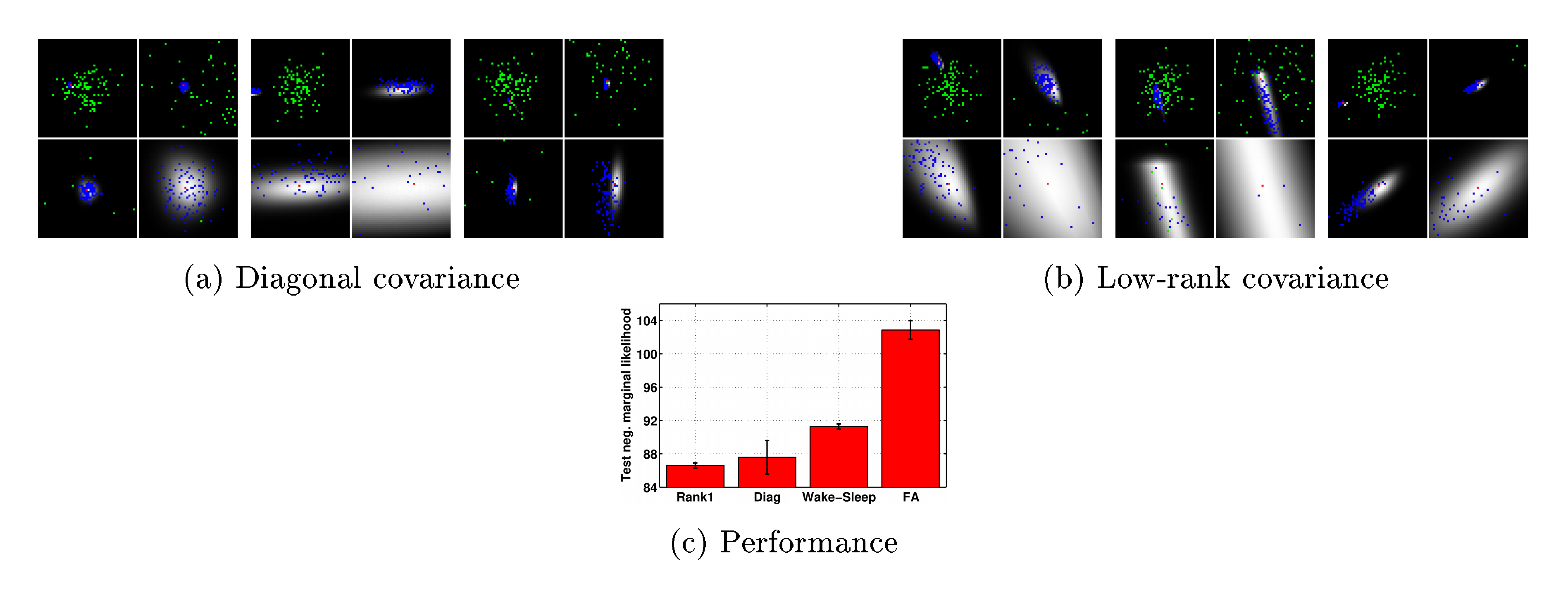
We use sampling to evaluate the true posterior distribution for a number of MNIST digits using the binarised data set from [21]. We visualise the posterior distribution for a model with two Gaussian latent variables in Figure 2. The true posterior distribution is shown by the grey regions and was computed by importance sampling with a large number of particles aligned in a grid between -5 and 5. In Figure 2(a) we see that these posterior distributions are elliptical or spherical in shape and thus, it is reasonable to assume that they can be well approximated by a Gaussian. Samples from the prior (green) are spread widely over the space and very few samples fall in the region of significant posterior mass, explaining the inefficiency of estimation methods that rely on samples from the prior. Samples from the recognition model (blue) are concentrated on the posterior mass, indicating that the recognition model has learnt the correct posterior statistics, which should lead to efficient learning.

\begin{tabular}{lc}
\hline
\textbf{Model} & $-\ln p(\mathbf{v})$ \\
\hline \hline
Factor Analysis & $106.00$ \\
NLGBN ([8]) & $95.80$ \\
Wake-Sleep ([10]) & 91.3\\
DLGM diagonal covariance & $87.30$ \\
DLGM rank-one covariance & $86.60$ \\
\hline
\multicolumn{2}{c}{\tiny\textit{Results below from [5]}} \\
MoBernoullis K=10 & 168.95 \\
MoBernoullis K=500 & 137.64 \\
RBM (500 h, 25 CD steps) approx. & 86.34\\
DBN 2hl approx. & 84.55\\
NADE 1hl (fixed order) & 88.86\\
NADE 1hl (fixed order, RLU, minibatch) & 88.33\\
EoNADE 1hl (2 orderings) & 90.69 \\
EoNADE 1hl (128 orderings) & 87.71 \\
EoNADE 2hl (2 orderings) & 87.96 \\
EoNADE 2hl (128 orderings) & 85.10 \\
\hline
\end{tabular}

In Figure 2(a) we see that samples from the recognition model are aligned to the axis and do not capture the posterior correlation. The correlation is captured using the structured covariance model in Figure 2(b). Not all posteriors are Gaussian in shape, but the recognition places mass in the best location possible to provide a reasonable approximation. As a benchmark for comparison, the performance in terms of test log-likelihood is shown in Figure 2(c), using the same architecture, for factor analysis (FA), the wake-sleep algorithm, and our approach using both the diagonal and structured covariance approaches. For this experiment, the generative model consists of 100 latent variables feeding into a deterministic layer of 300 nodes, which then feeds to the observation likelihood. We use the same structure for the recognition model.

5.2 Simulation and Prediction

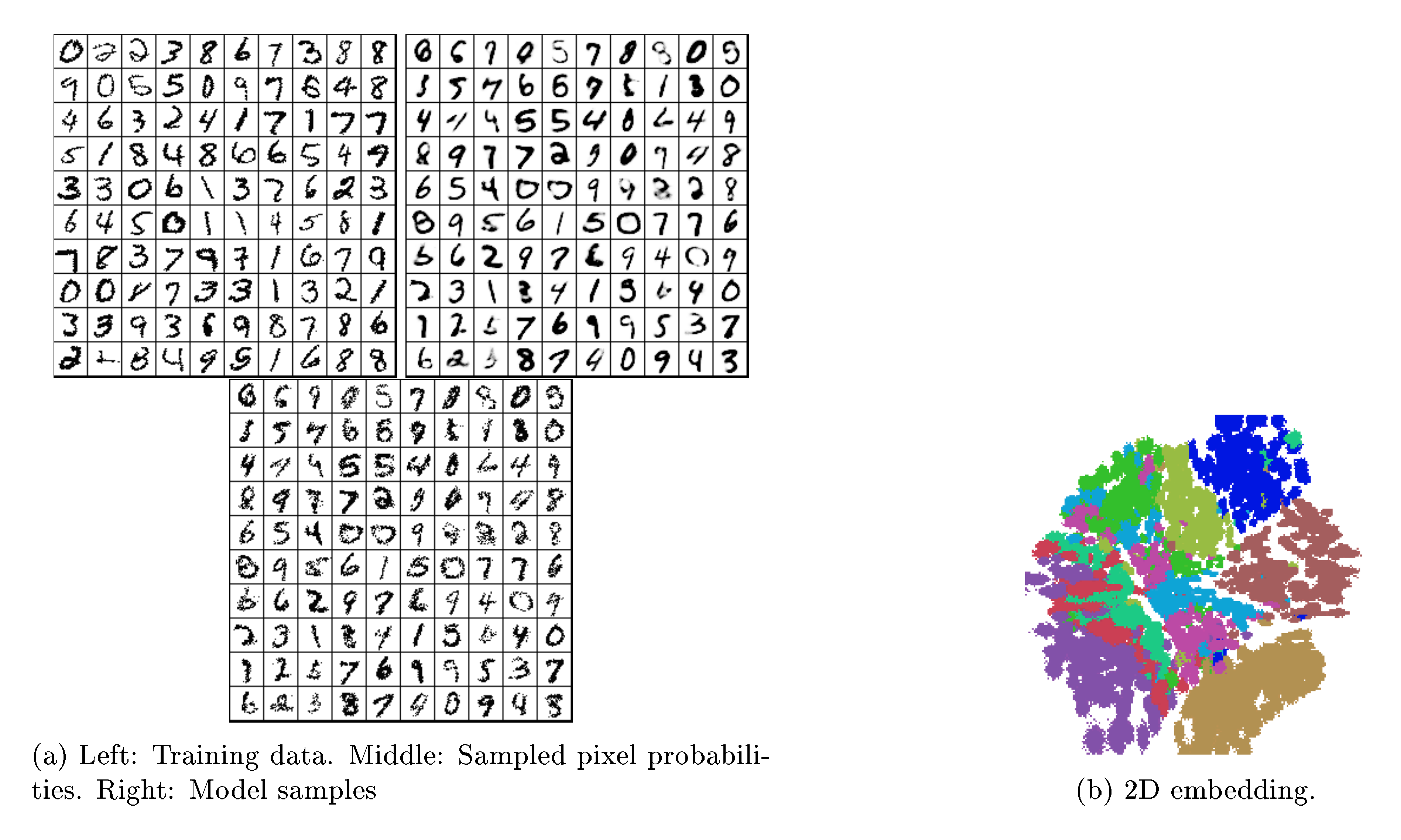
We evaluate the performance of a three layer latent Gaussian model on the MNIST data set. The model consists of two deterministic layers with 200 hidden units and a stochastic layer of 200 latent variables. We use mini-batches of 200 observations and trained the model using stochastic backpropagation. Samples from this model are shown in Figure 3a. We also compare the test log-likelihood to a large number of existing approaches in Table 1. We used the binarised dataset as in [5] and quote the log-likelihoods in the lower part of the table from this work. These results show that our approach is competitive with some of the best models currently available. The generated digits also match the true data well and visually appear as good as some of the best visualisations from these competing approaches.

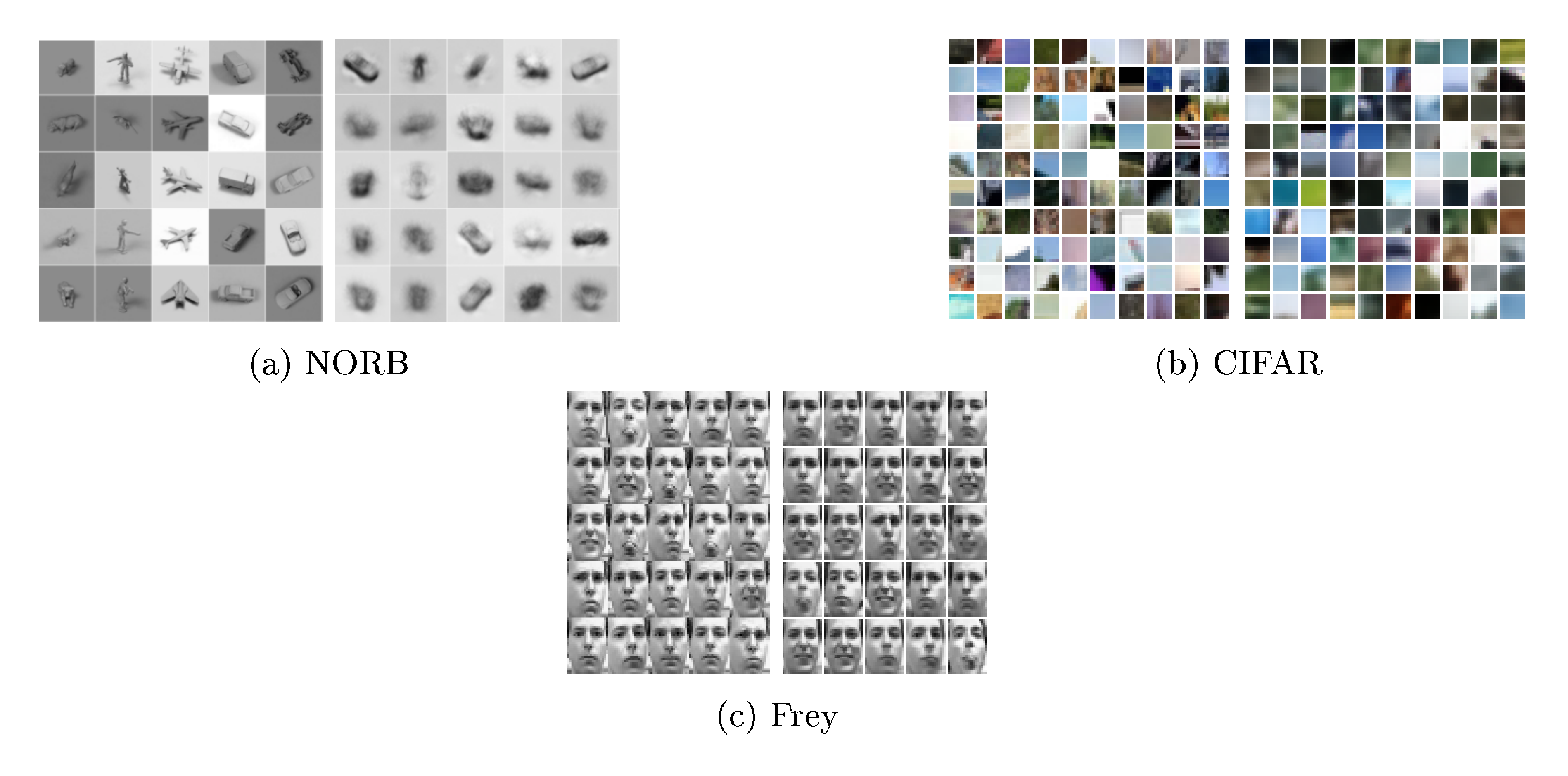
We also analysed the performance of our model on three high-dimensional real image data sets. The NORB object recognition data set consists of $24, 300$ images that are of size $96 \times 96$ pixels. We use a model consisting of 1 deterministic layer of 400 hidden units and one stochastic layer of 100 latent variables. Samples produced from this model are shown in Figure 4a. The CIFAR10 natural images data set consists of $50, 000$ RGB images that are of size $32 \times 32$ pixels, which we split into random $8 \times 8$ patches. We use the same model as used for the MNIST experiment and show samples from the model in Figure 4b. The Frey faces data set consists of almost $2, 000$ images of different facial expressions of size $28 \times 20$ pixels.

5.3 Data Visualisation

Latent variable models are often used for visualisation of high-dimensional data sets. We project the MNIST data set to a 2-dimensional latent space and use this 2D embedding as a visualisation of the data – an embedding for MNIST is shown in Figure 3b. The classes separate into different regions, suggesting that such embeddings can be useful in understanding the structure of high-dimensional data sets.

5.4 Missing Data Imputation and Denoising

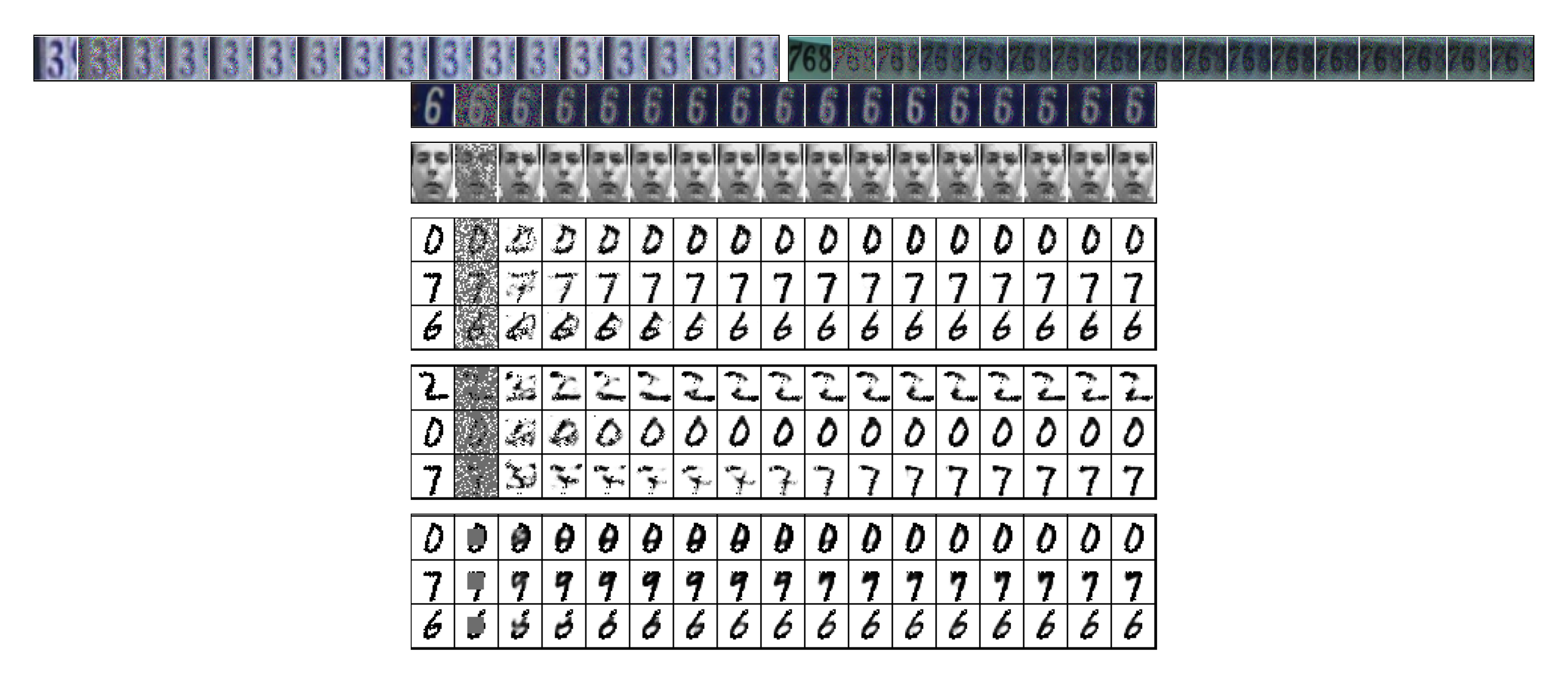
We demonstrate the ability of the model to impute missing data using the street view house numbers (SVHN) data set ([22]), which consists of $73, 257$ images of size $32 \times 32$ pixels, and the Frey faces and MNIST data sets. The performance of the model is shown in Figure 5.

We test the imputation ability under two different missingness types ([23]): Missing-at-Random (MAR), where we consider 60% and 80% of the pixels to be missing randomly, and Not Missing-at-Random (NMAR), where we consider a square region of the image to be missing. The model produces very good completions in both test cases. There is uncertainty in the identity of the image and this is reflected in the errors in these completions as the resampling procedure is run (see transitions from digit 9 to 7, and digit 8 to 6 in Figure 5). This further demonstrates the ability of the model to capture the diversity of the underlying data. We do not integrate over the missing values, but use a procedure that simulates a Markov chain that we show converges to the true marginal distribution of missing given observed pixels. The imputation procedure is discussed in Appendix F.

6. Discussion

Section Summary: The discussion outlines how Directed Graphical Models unify various existing approaches like factor analysis and Gaussian processes, while highlighting limitations in related methods such as neural auto-regressive estimators that struggle with high-dimensional data and deep structures. It argues that the proposed variational inference technique offers a scalable and effective way to handle latent Gaussian distributions, outperforming alternatives like Laplace approximations or expectation propagation, which are either inaccurate or computationally demanding. The section also favors their Monte Carlo variance reduction method for its efficiency over techniques like REINFORCE, and connects the model to denoising auto-encoders by interpreting them as a practical but less principled form of variational inference for generating samples.

Directed Graphical Models. DLGMs form a unified family of models that includes factor analysis ([4]), non-linear factor analysis ([7]), and non-linear Gaussian belief networks ([8]). Other related models include sigmoid belief networks ([3]) and deep auto-regressive networks ([6]), which use auto-regressive Bernoulli distributions at each layer instead of Gaussian distributions. The Gaussian process latent variable model and deep Gaussian processes ([24, 25]) form the non-parametric analogue of our model and employ Gaussian process priors over the non-linear functions between each layer. The neural auto-regressive density estimator (NADE) ([21, 5]) uses function approximation to model conditional distributions within a directed acyclic graph. NADE is amongst the most competitive generative models currently available, but has several limitations, such as the inability to allow for deep representations and difficulties in extending to locally-connected models (e.g., through the use of convolutional layers), preventing it from scaling easily to high-dimensional data.

Alternative latent Gaussian inference. Few of the alternative approaches for inferring latent Gaussian distributions meet the desiderata for scalable inference we seek. The Laplace approximation has been concluded to be a poor approximation in general, in addition to being computationally expensive. INLA is restricted to models with few hyperparameters (

lt;10$), whereas our interest is in 100s-1000s. EP cannot be applied to latent variable models due to the inability to match moments of the joint distribution of latent variables and model parameters. Furthermore, no reliable methods exist for moment-matching with means and covariances formed by non-linear transformations – linearisation and importance sampling are two, but are either inaccurate or very slow. Thus, the the variational approach we present remains a general-purpose and competitive approach for inference.

Monte Carlo variance reduction. Control variate methods are amongst the most general and effective techniques for variance reduction when Monte Carlo methods are used ([11]). One popular approach is the REINFORCE algorithm ([12]), since it is simple to implement and applicable to both discrete and continuous models, though control variate methods are becoming increasingly popular for variational inference problems ([13, 26, 27, 28]). Unfortunately, such estimators have the undesirable property that their variance scales linearly with the number of independent random variables in the target function, while the variance of GBP is bounded by a constant: for $K$-dimensional latent variables the variance of REINFORCE scales as $O(K)$, whereas GBP scales as $O(1)$ (see Appendix D).

An important family of alternative estimators is based on quadrature and series expansion methods ([29, 7]). These methods have low-variance at the price of introducing biases in the estimation. More recently a combination of the series expansion and control variate approaches has been proposed by [26].

A very general alternative is the wake-sleep algorithm ([1]). The wake-sleep algorithm can perform well, but it fails to optimise a single consistent objective function and there is thus no guarantee that optimising it leads to a decrease in the free energy Equation (6).

Relation to denoising auto-encoders. Denoising auto-encoders (DAE) ([30]) introduce a random corruption to the encoder network and attempt to minimize the expected reconstruction error under this corruption noise with additional regularisation terms. In our variational approach, the recognition distribution $q(\boldsymbol{\xi}| \mathbf{v})$ can be interpreted as a stochastic encoder in the DAE setting. There is then a direct correspondence between the expression for the free energy Equation (6) and the reconstruction error and regularization terms used in denoising auto-encoders (c.f. equation (4) of [31]). Thus, we can see denoising auto-encoders as a realisation of variational inference in latent variable models.

The key difference is that the form of encoding 'corruption' and regularisation terms used in our model have been derived directly using the variational principle to provide a strict bound on the marginal likelihood of a known directed graphical model that allows for easy generation of samples. DAEs can also be used as generative models by simulating from a Markov chain ([31, 32]). But the behaviour of these Markov chains will be very problem specific, and we lack consistent tools to evaluate their convergence.

7. Conclusion

Section Summary: This paper presents a versatile method for making inferences in models that involve hidden, continuous variables, using a special recognition model to efficiently process data like a probabilistic summary. It establishes a mathematical lower limit on the model's overall likelihood, incorporates modern deep learning techniques to shape and refine the recognition model, and adapts backpropagation rules to handle random elements, enabling the simultaneous tuning of all model parts. On various real-world datasets, the approach produces lifelike generated samples, reliably fills in missing information, and aids in visualizing complex, high-dimensional data.

We have introduced a general-purpose inference method for models with continuous latent variables. Our approach introduces a recognition model, which can be seen as a stochastic encoding of the data, to allow for efficient and tractable inference. We derived a lower bound on the marginal likelihood for the generative model and specified the structure and regularisation of the recognition model by exploiting recent advances in deep learning. By developing modified rules for backpropagation through stochastic layers, we derived an efficient inference algorithm that allows for joint optimisation of all parameters. We show on several real-world data sets that the model generates realistic samples, provides accurate imputations of missing data and can be a useful tool for high-dimensional data visualisation.

Appendices can be found with the online version of the paper. http://arxiv.org/abs/1401.4082

Acknowledgements. We are grateful for feedback from the reviewers as well as Peter Dayan, Antti Honkela, Neil Lawrence and Yoshua Bengio.

Appendix

Section Summary: The appendix delves into extra details about the generative model's mechanics, explaining how it transforms a basic spherical Gaussian distribution of noise into more complex ones that match real data through non-linear changes of coordinates, complete with supporting equations and simple examples of two-layer models and recognition processes. It also reviews proofs for key mathematical theorems, such as Bonnet's and Price's, which describe how gradients of expectations under Gaussian distributions can be swapped or expressed in terms of function derivatives, aiding in model training and analysis.

A. Additional Model Details

In equation 2ab we showed an alternative form of the joint log likelihood that explicitly separates the deterministic and stochastic parts of the generative model and corroborates the view that the generative model works by applying a complex non-linear transformation to a spherical Gaussian distribution $\mathcal{N}(\boldsymbol{\xi}| \boldsymbol{0}, \mathbf{I})$ such that the transformed distribution best matches the empirical distribution. We provide more details on this view here for clarity.

From the model description in equations 1ab and 1ac, we can interpret the variables $\mathbf{h}_l$ as deterministic functions of the noise variables $\boldsymbol{\xi}_l$. This can be formally introduced as a coordinate transformation of the probability density in equation 2aa: we perform a change of coordinates $\mathbf{h}l \rightarrow \boldsymbol{\xi}{l}$. The density of the transformed variables $\boldsymbol{\xi}_l$ can be expressed in terms of the density Equation (2aa) times the determinant of the Jacobian of the transformation $p(\boldsymbol{\xi}_l) = p(\mathbf{h}_l(\boldsymbol{\xi}_l)) |\frac{\partial \mathbf{h}_l}{\partial \boldsymbol{\xi}_l}|$. Since the co-ordinate transformation is linear we have $|\frac{\partial \mathbf{h}_l}{\partial \boldsymbol{\xi}_l}| = | \mathbf{G}_l|$ and the distribution of $\boldsymbol{\xi}_l$ is obtained as follows:

$ \begin{align} &p(\boldsymbol{\xi}_l)!! = p(\mathbf{h}_l(\boldsymbol{\xi}_l)) |\frac{\partial \mathbf{h}_l}{\partial \boldsymbol{\xi}_l}| \nonumber \ & p(\boldsymbol{\xi}_l)!! = ! p(\mathbf{h}_L) ! | \mathbf{G}L| ! \prod{l=1}^{L - 1} ! |! \mathbf{G}l!| p_l(\mathbf{h}l | \mathbf{h}{l+1}!) ! = !! \prod{l=1}^{L} ! | \mathbf{G}_l| | \mathbf{S}_l|^{-\frac{1}{2}} \mathcal{N}(\boldsymbol{\xi}l) \nonumber \ &= \prod{l=1}^{L} | \mathbf{G}_l| | \mathbf{G}_l \mathbf{G}_l^T|^{-\frac{1}{2}} \mathcal{N}(\boldsymbol{\xi}l | \boldsymbol{0}, \mathbf{I}) = \prod{l=1}^{L} \mathcal{N}!(\boldsymbol{\xi}_l | \boldsymbol{0}, \mathbf{I}). \end{align} $

Combining this equation with the distribution of the visible layer we obtain equation 2ab.

A.1 Examples

Below we provide simple, explicit examples of generative and recognition models.

In the case of a two-layer model the activation $\mathbf{h}1(\boldsymbol{\xi}{1, 2})$ in equation 2ab can be explicitly written as

$ \begin{align} \mathbf{h}1(\boldsymbol{\xi}{1, 2}) & = \mathbf{W}_1 f (\mathbf{G}_2 \boldsymbol{\xi}_2) + \mathbf{G}_1 \boldsymbol{\xi}_1 + \mathbf{b}_1. \end{align} $

Similarly, a simple recognition model consists of a single deterministic layer and a stochastic Gaussian layer with the rank-one covariance structure and is constructed as:

$ \begin{align} & q(\boldsymbol{\xi}l | \mathbf{v}) = \mathcal{N}\left(\boldsymbol{\xi}l | \boldsymbol{\mu}; (\textrm{diag}(\mathbf{d}) + \mathbf{u} \mathbf{u}^\top)^{-1}\right) \ & \boldsymbol{\mu} = \mathbf{W}\mu \mathbf{z} + \mathbf{b}\mu \ & \log \mathbf{d} = \mathbf{W}_d \mathbf{z} + \mathbf{b}_d ; \qquad \mathbf{u} = \mathbf{W}_u \mathbf{z} + \mathbf{b}_u \ & \mathbf{z} = f(\mathbf{W}_v \mathbf{v} + \mathbf{b}_v) \end{align} $

where the function $f$ is a rectified linearity (but other non-linearities such as tanh can be used).

[^2]

[^2]: Proceedings of the $\mathit{31}^{st}$ International Conference on Machine Learning, Beijing, China, 2014. JMLR: W&CP volume 32. Copyright 2014 by the author(s).

B. Proofs for the Gaussian Gradient Identities

Here we review the derivations of Bonnet's and Price's theorems that were presented in Section 3.

########## {caption="Bonnet's theorem" type="Theorem"}

Let $f(\boldsymbol{\xi}): R^d \mapsto R$ be a integrable and twice differentiable function. The gradient of the expectation of $f(\boldsymbol{\xi})$ under a Gaussian distribution $\mathcal{N}(\boldsymbol{\xi}| \boldsymbol{\mu}, \mathbf{C})$ with respect to the mean $\boldsymbol{\mu}$ can be expressed as the expectation of the gradient of $f(\boldsymbol{\xi})$.

$ \begin{align} \nabla_{\mu_i} \mathbb{E}{ \mathcal{N}(\mu, \mathbf{C}) } \left[f(\boldsymbol{\xi}) \right] &= \mathbb{E}{ \mathcal{N}(\boldsymbol{\mu}, \mathbf{C}) } \left[\nabla_{\xi_i} f(\boldsymbol{\xi}) \right], \nonumber \end{align} $

Proof:

$ \begin{align} \nabla_{\mu_i} \mathbb{E}{ \mathcal{N}(\boldsymbol{\mu}, \mathbf{C}) } \left[f(\boldsymbol{\xi}) \right] &= \int \nabla{\mu_i} \mathcal{N}(\boldsymbol{\xi}| \boldsymbol{\mu}, \mathbf{C}) f(\boldsymbol{\xi}) d \boldsymbol{\xi} \nonumber \ &= -\int \nabla_{\xi_i} \mathcal{N}(\boldsymbol{\xi}| \boldsymbol{\mu}, \mathbf{C}) f(\boldsymbol{\xi}) d \boldsymbol{\xi} \nonumber \ &= \left[\int \mathcal{N}(\boldsymbol{\xi}| \boldsymbol{\mu}, \mathbf{C}) f(\boldsymbol{\xi}) d \boldsymbol{\xi}{\neg i} \right] { \xi_i = -\infty }^{\xi_i = + \infty} \nonumber \ &+ \int \mathcal{N}(\boldsymbol{\xi}| \boldsymbol{\mu}, \mathbf{C}) \nabla{\xi_i} f(\boldsymbol{\xi}) d \boldsymbol{\xi} \nonumber \ &= \mathbb{E}{ \mathcal{N}(\boldsymbol{\mu}, \mathbf{C}) } \left[\nabla_{\xi_i} f(\boldsymbol{\xi}) \right], \end{align} $

where we have used the identity

$ \begin{align} \nabla_{\mu_i} \mathcal{N}(\boldsymbol{\xi}| \boldsymbol{\mu}, \mathbf{C}) &= - \nabla_{\xi_i} \mathcal{N}(\boldsymbol{\xi}| \boldsymbol{\mu}, \mathbf{C}) \nonumber \end{align} $

in moving from step 1 to 2. From step 2 to 3 we have used the product rule for integrals with the first term evaluating to zero.

########## {caption="Price's theorem" type="Theorem"}

Under the same conditions as before. The gradient of the expectation of $f(\boldsymbol{\xi})$ under a Gaussian distribution $\mathcal{N}(\boldsymbol{\xi}| \boldsymbol{0}, \mathbf{C})$ with respect to the covariance $\mathbf{C}$ can be expressed in terms of the expectation of the Hessian of $f(\boldsymbol{\xi})$ as

$ \begin{align} \nabla_{C_{i, j}} \mathbb{E}{ \mathcal{N}(\boldsymbol{0}, C) } \left[f(\boldsymbol{\xi}) \right] &= \frac{1}{2} \mathbb{E}{ \mathcal{N}(\boldsymbol{0}, C) } \left[\nabla_{\xi_i, \xi_j} f(\boldsymbol{\xi}) \right] \nonumber \end{align} $

Proof:

$ \begin{align} \nabla_{C_{i, j}} \mathbb{E}{ \mathcal{N}(\boldsymbol{0}, \mathbf{C}) } \left[f(\boldsymbol{\xi}) \right] &= \int \nabla{C_{i, j}} \mathcal{N}(\boldsymbol{\xi}| \boldsymbol{0}, \mathbf{C}) f(\boldsymbol{\xi}) d \boldsymbol{\xi} \nonumber \ &= \frac{1}{2} \int \nabla_{\xi_i, \xi_j} \mathcal{N}(\boldsymbol{\xi}| \boldsymbol{0}, \mathbf{C}) f(\boldsymbol{\xi}) d \boldsymbol{\xi} \nonumber \ &= \frac{1}{2} \int \mathcal{N}(\boldsymbol{\xi}| \boldsymbol{0}, \mathbf{C}) \nabla_{\xi_i, \xi_j} f(\boldsymbol{\xi}) d \boldsymbol{\xi} \nonumber \ &= \frac{1}{2} \mathbb{E}{ \mathcal{N}(\boldsymbol{0}, \mathbf{C}) } \left[\nabla{\xi_i, \xi_j} f(\boldsymbol{\xi}) \right]. \end{align} $

In moving from steps 1 to 2, we have used the identity

$ \begin{align} \nabla_{C_{i, j}} \mathcal{N}(\boldsymbol{\xi}| \mu, \mathbf{C}) &= \frac{1}{2} \nabla_{\xi_i, \xi_j} \mathcal{N}(\boldsymbol{\xi}| \mu, \mathbf{C}), \nonumber \end{align} $

which can be verified by taking the derivatives on both sides and comparing the resulting expressions. From step 2 to 3 we have used the product rule for integrals twice.

C. Deriving Stochastic Back-propagation Rules

In Section 3 we described two ways in which to derive stochastic back-propagation rules. We show specific examples and provide some more discussion in this section.

C.1 Using the Product Rule for Integrals

We can derive rules for stochastic back-propagation for many distributions by finding a appropriate non-linear function $B(x; \theta)$ that allows us to express the gradient with respect to the parameters of the distribution as a gradient with respect to the random variable directly. The approach we described in the main text was:

$ \begin{align} & \nabla_{\theta} \mathbb{E}{p} [f(x)] !=!! \int !\nabla{\theta} p (!x | \theta)! f!(!x!) d x !=!! \int !\nabla_x p (!x | \theta) B (!x!) f!(!x!) d x \nonumber \ & = [B (x) f (x) p (x | \theta)] {supp (x)} - \int p (x | \theta) \nabla_x [B (x) f (x)] \nonumber \ & = - \mathbb{E}{p (x | \theta)} [\nabla_x [B (x) f (x)]] \end{align}\tag{16} $

where we have introduced the non-linear function $B(x;\theta)$ to allow for the transformation of the gradients and have applied the product rule for integrals (rule for integration by parts) to rewrite the integral in two parts in the second line, and the supp $(x)$ indicates that the term is evaluated at the boundaries of the support. To use this approach, we require that the density we are analysing be zero at the boundaries of the support to ensure that the first term in the second line is zero.

As an alternative, we can also write this differently and find an non-linear function of the form:

$ \begin{align} \nabla_{\theta} \mathbb{E}{p} [f(x)] !=!! = - \mathbb{E}{p (x | \theta)} [B (x) \nabla_x f (x)]. \end{align} $

Consider general exponential family distributions of the form:

$ \begin{align} p (x | \theta) = h (x) \exp (\eta (\theta)^\top \phi (x) - A(\theta)) \end{align} $

where $h(x)$ is the base measure, $\theta$ is the set of mean parameters of the distribution, $\eta$ is the set of natural parameters, and $A(\theta)$ is the log-partition function. We can express the non-linear function in Equation 16 using these quantities as:

$ \begin{align} B(x) = \frac{[\nabla_{\theta} \eta (\theta) \phi (x) - \nabla_{\theta} A (\theta)]}{[\nabla_x \log [h (x)] + \eta (\theta)^T \nabla_x \phi (x)]}. \end{align} $

This can be derived for a number of distributions such as the Gaussian, inverse Gamma, Log-Normal, Wald (inverse Gaussian) and other distributions. We show some of these below:

Family	$\theta$	$B(x)$
Gaussian	$\left(\begin{array}{c}\mu sigma^2 \end{array}\right)$	$\left(\begin{array}{c} - 1\ \frac{(x - \mu - \sigma^{}) (x - \mu + \sigma)^{}}{2 \sigma^2 (x - \mu)} \end{array}\right)$
Inv. Gamma	$\left(\begin{array}{c}\alpha beta \end{array}\right)$	$\left(\begin{array}{c} \frac{x^2(- \ln x - \Psi (\alpha) + \ln \beta)}{- x (\alpha + 1) + \beta}\ (\frac{x^2}{- x (\alpha + 1) + \beta})(- \frac{1}{x} + \frac{\alpha}{\beta}) \end{array}\right)$
Log-Normal	$\left(\begin{array}{c}\mu sigma^2 \end{array}\right)$	$\left(\begin{array}{c} - 1\ \frac{(\ln x - \mu - \sigma^{}) (\ln x - \mu + \sigma)^{}}{2 \sigma^2 (\ln x - \mu)} \end{array}\right)$

The $B(x ;\theta)$ corresponding to the second formulation can also be derived and may be useful in certain situations, requiring the solution of a first order differential equation. This approach of searching for non-linear transformations leads us to the second approach for deriving stochastic back-propagation rules.

C.2 Using Alternative Coordinate Transformations

There are many distributions outside the exponential family that we would like to consider using. A simpler approach is to search for a co-ordinate transformation that allows us to separate the deterministic and stochastic parts of the distribution. We described the case of the Gaussian in Section 3. Other distributions also have this property. As an example, consider the Levy distribution (which is a special case of the inverse Gamma considered above). Due to the self-similarity property of this distribution, if we draw $X$ from a Levy distribution with known parameters $X \sim \textrm{Levy}(\mu, \lambda)$, we can obtain any other Levy distribution by rescaling and shifting this base distribution: $kX + b \sim \textrm{Levy}(k\mu + b, kc)$.

Many other distributions hold this property, allowing stochastic back-propagation rules to be determined for distributions such as the Student's t-distribution, Logistic distribution, the class of stable distributions and the class of generalised extreme value distributions (GEV). Examples of co-ordinate transformations $T(\cdot)$ and the resulsting distributions are shown below for variates $X$ drawn from the standard distribution listed in the first column.

Std Distr.	T $(\cdot)$	Gen. Distr.
GEV $(\mu, \sigma, 0)$	$mX !+! b$	GEV $(m\mu !+! b, m \sigma, 0)$
Exp $(1)$	$\mu !+! \beta! \ln(1 !+! \exp(-!X))$	Logistic $(\mu, \beta)$
Exp $(1)$	$\lambda X^{\frac{1}{k}}$	Weibull $(\lambda, k)$

D. Variance Reduction using Control Variates

An alternative approach for stochastic gradient computation is commonly based on the method of control variates. We analyse the variance properties of various estimators in a simple example using univariate function. We then show the correspondence of the widely-known REINFORCE algorithm to the general control variate framework.

D.1 Variance discussion for REINFORCE

The REINFORCE estimator is based on

$ \begin{align} \nabla_{\theta} \mathbb{E}_p [f(\xi)] &= \mathbb{E}_p [(f(\xi) - b) \nabla _{\theta} \log p(\xi | \theta)],

\end{align}\tag{17} $

where $b$ is a baseline typically chosen to reduce the variance of the estimator.

The variance of Equation 17 scales poorly with the number of random variables ([1]). To see this limitation, consider functions of the form $f(\xi) = \sum_{i=1}^K f(\xi_i)$, where each individual term and its gradient has a bounded variance, i.e., $\kappa_l \leq \textrm{Var}[f(\xi_i)] \leq \kappa_u$ and $\kappa_l \leq \textrm{Var}[\nabla_{\xi_i}f(\xi_i)] \leq \kappa_u$ for some $0\leq \kappa_{l} \leq \kappa_u$ and assume independent or weakly correlated random variables. Given these assumptions the variance of GBP Equation 3aa scales as $\textrm{Var}[\nabla_{\xi_i} f(\xi)] \sim O(1)$, while the variance for REINFORCE Equation 17 scales as $\textrm{Var}\left[\frac{(\xi_i - \mu_i)}{ \sigma_i^2 } (f(\xi) - \mathbb{E}[f(\xi)]) \right] \sim O(K).$ \

For the variance of GBP above, all terms in $f(\xi)$ that do not depend on $\xi_i$ have zero gradient, whereas for REINFORCE the variance involves a summation over all $K$ terms. Even if most of these terms have zero expectation, they still contribute to the variance of the estimator. Thus, the REINFORCE estimator has the undesirable property that its variance scales linearly with the number of independent random variables in the target function, while the variance of GBP is bounded by a constant.

The assumption of weakly correlated terms is relevant for variational learning in larger generative models where independence assumptions and structure in the variational distribution result in free energies that are summations over weakly correlated or independent terms.

D.2 Univariate variance analysis

In analysing the variance properties of many estimators, we discuss the general scaling of likelihood ratio approaches in Appendix D. As an example to further emphasise the high-variance nature of these alternative approaches, we present a short analysis in the univariate case.

Consider a random variable $p(\xi) = \mathcal{N}(\xi| \mu, \sigma^2)$ and a simple quadratic function of the form

$ \begin{align} f(\xi) &= c \frac{\xi^2}{2}. \end{align} $

For this function we immediately obtain the following variances

$ \begin{align} Var[\nabla_{\xi} f(\xi)] &= c^2 \sigma^2 \tag{a} \ Var[\nabla_{\xi^2} f(\xi)] &= 0 \tag{b} \ Var[\frac{(\xi - \mu)}{ \sigma } \nabla_{\xi} f(\xi)] &= 2 c^2 \sigma^2 + \mu^2 c^2 \tag{c} \ Var[\frac{(\xi - \mu)}{ \sigma^2 } (f(\xi) - \mathbb{E}[f(\xi)])] &= 2 c^2 \mu^2 + \frac{5}{2} c^2 \sigma^2 \tag{d} \end{align}\tag{18} $

Equations 18aa, Equation 18ab and 18ac correspond to the variance of the estimators based on Equation 3aa, Equation 3ab, Equation 5 respectively whereas equation 18ad corresponds to the variance of the REINFORCE algorithm for the gradient with respect to $\mu$.

From these relations we see that, for any parameter configuration, the variance of the REINFORCE estimator is strictly larger than the variance of the estimator based on Equation 3aa. Additionally, the ratio between the variances of the former and later estimators is lower-bounded by $5/2$. We can also see that the variance of the estimator based on equation 3ab is zero for this specific function whereas the variance of the estimator based on equation 5 is not.

E. Estimating the Marginal Likelihood

We compute the marginal likelihood by importance sampling by generating $S$ samples from the recognition model and using the following estimator:

$ \begin{align} p(\mathbf{v}) & \approx \frac{1}{S} \sum_{s = 1}^S \frac{p(\mathbf{v} | \mathbf{h}(\boldsymbol{\xi}^{(s)})) p(\boldsymbol{\xi}^{(s)})}{q(\boldsymbol{\xi}^{s}| \mathbf{v})} ; \quad \boldsymbol{\xi}^{(s)}\sim q(\boldsymbol{\xi} | \mathbf{v}) \end{align}\tag{19} $

F. Missing Data Imputation

Image completion can be approximatively achieved by a simple iterative procedure which consists of (i) initializing the non-observed pixels with random values; (ii) sampling from the recognition distribution given the resulting image; (iii) reconstruct the image given the sample from the recognition model; (iv) iterate the procedure.

We denote the observed and missing entries in an observation as $\mathbf{v}_o, \mathbf{v}_m$, respectively. The observed $\mathbf{v}_o$ is fixed throughout, therefore all the computations in this section will be conditioned on $\mathbf{v}_o$. The imputation procedure can be written formally as a Markov chain on the space of missing entries $\mathbf{v}_m$ with transition kernel $T^q(\mathbf{v}'_m | \mathbf{v}_m, \mathbf{v}_o)$ given by

$ \begin{align} T^q(\mathbf{v}'_m | \mathbf{v}_m, \mathbf{v}_o) &= \iint p(\mathbf{v}'_m, \mathbf{v}'_o | \xi) q(\xi| \mathbf{v}) d \mathbf{v}'_o d \xi, \end{align}\tag{20} $

where $\mathbf{v} = (\mathbf{v}_m, \mathbf{v}_o)$.

Provided that the recognition model $q(\xi| \mathbf{v})$ constitutes a good approximation of the true posterior $p(\xi| \mathbf{v})$, Equation 20 can be seen as an approximation of the kernel

$ \begin{align} T(\mathbf{v}'_m | \mathbf{v}_m, \mathbf{v}_o) &= \iint p(\mathbf{v}'_m, \mathbf{v}'_o | \xi) p(\xi| \mathbf{v}) d \mathbf{v}'_o d \xi. \end{align}\tag{21} $

The kernel Equation 21 has two important properties: (i) it has as its eigen-distribution the marginal $p(\mathbf{v}_m| \mathbf{v}_o)$; (ii) $T(\mathbf{v}'_m | \mathbf{v}_m, \mathbf{v}_o) > 0 \forall \mathbf{v}_o, \mathbf{v}_m, \mathbf{v}'_m$. The property (i) can be derived by applying the kernel Equation 21 to the marginal $p(\mathbf{v}_m| \mathbf{v}_o)$ and noting that it is a fixed point. Property (ii) is an immediate consequence of the smoothness of the model.

We apply the fundamental theorem for Markov chains ([?], pp. 38) and conclude that given the above properties, a Markov chain generated by Equation 21 is guaranteed to generate samples from the correct marginal $p(\mathbf{v}_m| \mathbf{v}_o)$.

In practice, the stationary distribution of the completed pixels will not be exactly the marginal $p(\mathbf{v}_m| \mathbf{v}_o)$, since we use the approximated kernel Equation 20. Even in this setting we can provide a bound on the $L_1$ norm of the difference between the resulting stationary marginal and the target marginal $p(\mathbf{v}_m| \mathbf{v}_o)$

########## {caption=" $L_1$ bound on marginal error" type="Proposition"}

If the recognition model $q (\xi | \mathbf{v})$ is such that for all $\xi$

$ \begin{align} \exists \varepsilon >0 \textrm{ s.t. } \int \left| \frac{q(\xi | \mathbf{v}) p(\mathbf{v})}{p(\xi)} - p (\mathbf{v} | \xi) \right| d \mathbf{v} \leq \varepsilon \end{align}\tag{22} $

then the marginal $p(\mathbf{v}_m| \mathbf{v}_o)$ is a weak fixed point of the kernel Equation 20 in the following sense:

$ \begin{split} \int \Bigg| \int \big(T^q(\mathbf{v}'_m | \mathbf{v}_m, \mathbf{v}_o) - \ T(\mathbf{v}'_m | \mathbf{v}_m, \mathbf{v}_o)\big)\ p(\mathbf{v}_m| \mathbf{v}_o) d \mathbf{v}_m \Bigg| d \mathbf{v}'_m < \varepsilon. \end{split}\tag{23} $

Proof:

$ \begin{align} & \int ! \left| ! \int !\left[T^q(\mathbf{v}'_m | \mathbf{v}_m, \mathbf{v}_o) !-! T(\mathbf{v}'_m | \mathbf{v}_m, \mathbf{v}_o)\right] p(\mathbf{v}_m| \mathbf{v}_o) d \mathbf{v}_m \right | d \mathbf{v}'_m \nonumber\ = & \int | \iint p (\mathbf{v}'_m, \mathbf{v}'_o | \xi) p (\mathbf{v}_m, \mathbf{v}_o) [q (\xi | \mathbf{v}_m, \mathbf{v}_o) \nonumber\

• & p (\xi | \mathbf{v}_m, \mathbf{v}_o)] d \mathbf{v}_m d \xi | d \mathbf{v}'_m \nonumber \ = & \int \left | \int p (\mathbf{v}' | \xi) p (\mathbf{v}) [q (\xi | \mathbf{v}) - p (\xi | \mathbf{v})] \frac{p(\mathbf{v})}{p(\xi)} \frac{p(\xi)}{p(\mathbf{v})} d \mathbf{v} d \xi \right| d \mathbf{v}' \nonumber \ = & \int \left | \int p (\mathbf{v}' | \xi) p (\xi) [q (\xi | \mathbf{v}) \frac{p(\mathbf{v})}{p(\xi)} - p (\mathbf{v} | \xi)] d \mathbf{v} d \xi \right| d \mathbf{v}' \nonumber \ \leq & \int \int p (\mathbf{v}' | \xi) p (\xi) \int \left | q (\xi | \mathbf{v}) \frac{p(\mathbf{v})}{p(\xi)} - p (\mathbf{v} | \xi) \right| d \mathbf{v} d \xi d \mathbf{v}' \nonumber \ \leq & \varepsilon, \nonumber \end{align} $

where we apply the condition Equation 22 to obtain the last statement.

That is, if the recognition model is sufficiently close to the true posterior to guarantee that Equation 22 holds for some acceptable error $\varepsilon$ than Equation 23 guarantees that the fixed-point of the Markov chain induced by the kernel Equation 20 is no further than $\varepsilon$ from the true marginal with respect to the $L_1$ norm.

G. Variational Bayes for Deep Directed Models

In the main test we focussed on the variational problem of specifying an posterior on the latent variables only. It is natural to consider the variational Bayes problem in which we specify an approximate posterior for both the latent variables and model parameters.

Following the same construction and considering an Gaussian approximate distribution on the model parameters $\boldsymbol{\theta}^g$, the free energy becomes:

$ \begin{align} \mathcal{F}(\mathbf{V}) &= -\sum_n \overbrace{\mathbb{E}{q}{ \left[\log p(\mathbf{v}n| \mathbf{h}(\boldsymbol{\xi}n)) \right] }}^{\text{reconstruction error}} \nonumber \ &+ \underbrace{\frac{1}{2} \sum{n, l} \left[\Vert \boldsymbol{\mu}{n, l} \Vert ^2 + \operatorname{Tr} \mathbf{C} {n, l} - \log \vert \mathbf{C}{n, l} \vert - 1 \right] }{\text{latent regularization term}}\nonumber \ &+\underbrace{\frac{1}{2}\sum_j \left[\frac{m_j^2}{\kappa} + \frac{\tau_j}{\kappa} + \log \kappa - \log \tau_j - 1 \right]}_{\text{parameter regularization term}}, \end{align}\tag{24} $

which now includes an additional term for the cost of using parameters and their regularisation. We must now compute the additional set of gradients with respect to the parameter's mean $m_j$ and variance $\tau_j$ are:

$ \begin{align} \nabla_{m_j} \mathcal{F}(\mathbf{v}) &= -\mathbb{E}{q}\left[\nabla{\theta_j^g} \log p(\mathbf{v} | \mathbf{h}(\boldsymbol{\xi}))\right] + m_j\ \nabla_{\tau_j} \mathcal{F}(\mathbf{v}) &= - \tfrac{1}{2}\mathbb{E}{q} \left[\frac{\theta_j - m_j}{\tau_j} \nabla{\theta_j^g} \log p(\mathbf{v}| \mathbf{h}(\xi)) \right] \nonumber\ &+ \frac{1}{2 \kappa} - \frac{1}{2 \tau_j} \end{align}\tag{25} $

H. Additional Simulation Details

We use training data of various types including binary and real-valued data sets. In all cases, we train using mini-batches, which requires the introduction of scaling terms in the free energy objective function Equation 8 in order to maintain the correct scale between the prior over the parameters and the remaining terms ([?, ?]). We make use of the objective:

$ \begin{align} & \overline{\mathcal{F}(\mathbf{V})} = -\lambda \sum_n \mathbb{E}_{q} \left[\log p(\mathbf{v}_n| \mathbf{h}(\boldsymbol{\xi}_n)) \right]

• \tfrac{1}{2 \kappa} \Vert \boldsymbol{\theta}^g\Vert ^2 \nonumber \ &+ \frac{\lambda}{2} \sum_{n, l} \left[\Vert \boldsymbol{\mu}_{n, l} \Vert ^2 + \operatorname{Tr}(\mathbf{C} {n, l}) - \log \vert \mathbf{C}{n, l} \vert - 1 \right], \end{align}\tag{26} $

where $n$ is an index over observations in the mini-batch and $\lambda$ is equal to the ratio of the data-set and the mini-batch size. At each iteration, a random mini-batch of size 200 observations is chosen.

All parameters of the model were initialized using samples from a Gaussian distribution with mean zero and variance $1\times 10^6$; the prior variance of the parameters was $\kappa = 1\times 10^6$. We compute the marginal likelihood on the test data by importance sampling using samples from the recognition model; we describe our estimator in Appendix E.

References

[1] Dayan, P., Hinton, G. E., Neal, R. M., and Zemel, R. S. The Helmholtz machine. Neural computation, 7(5):889–904, September 1995.

[2] Frey, B. J. Variational inference for continuous sigmoidal Bayesian networks. In Proceedings of the International Conference on Artificial Intelligence and Statistics (AISTATS), 1996.

[3] Saul, L. K., Jaakkola, T., and Jordan, M. I. Mean field theory for sigmoid belief networks. Journal of Artificial Intelligence Research (JAIR), 4:61–76, 1996.

[4] Bartholomew, D. J. and Knott, M. Latent variable models and factor analysis, volume 7 of Kendall's library of statistics. Arnold, 2nd edition, 1999.

[5] Uria, B., Murray, I., and Larochelle, H. A deep and tractable density estimator. In Proceedings of the International Conference on Machine Learning (ICML), 2014.

[6] Gregor, K., Mnih, A., and Wierstra, D. Deep autoregressive networks. In Proceedings of the International Conference on Machine Learning (ICML), October 2014.

[7] Lappalainen, H. and Honkela, A. Bayesian non-linear independent component analysis by multi-layer perceptrons. In Advances in independent component analysis (ICA), pp.\ 93–121. Springer, 2000.

[8] Frey, B. J. and Hinton, G. E. Variational learning in nonlinear Gaussian belief networks. Neural Computation, 11(1):193–213, January 1999.

[9] Beal, M. J. Variational Algorithms for approximate Bayesian inference. PhD thesis, University of Cambridge, 2003.

[10] Dayan, P. Helmholtz machines and wake-sleep learning. Handbook of Brain Theory and Neural Network. MIT Press, Cambridge, MA, 44(0), 2000.

[11] Wilson, J. R. Variance reduction techniques for digital simulation. American Journal of Mathematical and Management Sciences, 4(3):277–312, 1984.

[12] Williams, R. J. Simple statistical gradient-following algorithms for connectionist reinforcement learning. Machine Learning, 8:229 – 256, 1992.

[13] Hoffman, M., Blei, D. M., Wang, C., and Paisley, J. Stochastic variational inference. Journal of Machine Learning Research, 14:1303–1347, May 2013.

[14] Bonnet, G. Transformations des signaux aléatoires a travers les systèmes non linéaires sans mémoire. Annales des Télécommunications, 19(9-10):203–220, 1964.

[15] Price, R. A useful theorem for nonlinear devices having Gaussian inputs. IEEE Transactions on Information Theory, 4(2):69–72, 1958.

[16] Opper, M. and Archambeau, C. The variational Gaussian approximation revisited. Neural computation, 21(3):786–92, March 2009.

[17] Graves, A. Practical variational inference for neural networks. In Advances in Neural Information Processing Systems 24 (NIPS), pp.\ 2348–2356, 2011.

[18] Kingma, D. P. and Welling, M. Auto-encoding variational Bayes. Proceedings of the International Conference on Learning Representations (ICLR), 2014.

[19] Gershman, S. J. and Goodman, N. D. Amortized inference in probabilistic reasoning. In Proceedings of the 36th Annual Conference of the Cognitive Science Society, 2014.

[20] Magdon-Ismail, M. and Purnell, J. T. Approximating the covariance matrix of GMMs with low-rank perturbations. In Proceedings of the 11th international conference on Intelligent data engineering and automated learning (IDEAL), pp.\ 300–307, 2010.

[21] Larochelle, H. and Murray, I. The neural autoregressive distribution estimator. In Proceedings of the International Conference on Artificial Intelligence and Statistics (AISTATS), 2011.

[22] Netzer, Y., Wang, T., Coates, A., Bissacco, A., Wu, B., and Ng, A. Y. Reading digits in natural images with unsupervised feature learning. In NIPS Workshop on Deep Learning and Unsupervised Feature Learning, 2011.

[23] Little, R. J. and Rubin, D. B. Statistical analysis with missing data, volume 539. Wiley New York, 1987.

[24] Lawrence, N. Probabilistic non-linear principal component analysis with Gaussian process latent variable models. The Journal of Machine Learning Research, 6:1783–1816, 2005.

[25] Damianou, A. C. and Lawrence, N. D. Deep Gaussian processes. In Proceedings of the International Conference on Artificial Intelligence and Statistics (AISTATS), 2013.

[26] Blei, D. M., Jordan, M. I., and Paisley, J. W. Variational Bayesian inference with stochastic search. In Proceedings of the 29th International Conference on Machine Learning (ICML), pp.\ 1367–1374, 2012.

[27] Ranganath, R., Gerrish, S., and Blei, D. M. Black box variational inference. In Proceedings of the International Conference on Artificial Intelligence and Statistics (AISTATS), October 2014.

[28] Salimans, T. and Knowles, D. A. On using control variates with stochastic approximation for variational bayes and its connection to stochastic linear regression. ArXiv preprint. arXiv:1401.1022, October 2014.

[29] Honkela, A. and Valpola, H. Unsupervised variational Bayesian learning of nonlinear models. In Advances in Neural Information Processing Systems (NIPS), 2004.

[30] Vincent, P., Larochelle, H., Lajoie, I., Bengio, Y., and Manzagol, P. Stacked denoising autoencoders: Learning useful representations in a deep network with a local denoising criterion. The Journal of Machine Learning Research, 11:3371–3408, 2010.

[31] Bengio, Y., Yao, L., Alain, G., and Vincent, P. Generalized denoising auto-encoders as generative models. In Advances in Neural Information Processing Systems (NIPS), pp.\ 1–9, 2013.

[32] Bengio, Y. and Thibodeau-Laufer, É. Deep generative stochastic networks trainable by backprop. Technical report, University of Montreal, 2013.