Executive Summary: In the field of artificial intelligence, particularly for visual recognition tasks like image classification, a key challenge is scaling up neural network models to improve accuracy without a proportional explosion in computational costs. Larger models, such as vision transformers (ViTs), deliver better performance but require vast resources for training and inference, making them impractical for widespread deployment on devices or in real-time applications. This issue is pressing now as demand grows for efficient AI in areas like medical imaging, autonomous vehicles, and content moderation, where speed and cost directly impact feasibility and scalability.
This paper introduces and evaluates Soft MoE, a new type of mixture of experts (MoE) architecture for vision transformers. The goal is to demonstrate how Soft MoE can expand model capacity and performance while keeping training and inference costs low, addressing limitations in existing sparse MoE methods like training instability and inefficient token assignments.
The authors developed Soft MoE as a fully differentiable alternative to traditional sparse MoEs, which rely on discrete routing decisions between input tokens and specialized "expert" sub-modules. Instead, Soft MoE uses soft weighting to blend tokens before passing weighted combinations to experts, ensuring all inputs contribute fractionally without dropping any. They trained and tested models on JFT-4B, a massive dataset of over 4 billion images across 29,000 classes, over periods up to 10 million steps with batch sizes of 4,096 images. Comparisons involved dense ViTs and popular sparse MoEs (Tokens Choice and Experts Choice) across sizes from small (33 million parameters) to huge (54 billion parameters), evaluating on upstream accuracy, few-shot learning on ImageNet (using just 10 examples per class), full ImageNet fine-tuning, and image-text contrastive tasks on datasets like WebLI and LAION-400M. Key assumptions included replacing half the model's feedforward layers with Soft MoE blocks and using one slot (input blend) per expert for optimal efficiency.
The core findings highlight Soft MoE's superiority. First, it achieves higher accuracy than dense ViTs and other sparse MoEs for the same training compute budget; for instance, Soft MoE small models reach performance levels of large dense ViTs using half the training time. Second, inference speed is dramatically improved: a Soft MoE base model (3.7 billion parameters) matches a dense huge ViT (669 million parameters) on few-shot and fine-tuning tasks but runs 5.7 times faster, with 10 times fewer floating-point operations per image. Third, Soft MoE scales effectively to extreme sizes—a huge variant with 128 experts and 54 billion parameters outperforms its dense counterpart by a wide margin while increasing inference time by just 2 percent. Fourth, it avoids common pitfalls like token dropping or expert imbalances, enabling stable training even with thousands of experts. Finally, benefits extend beyond classification: in image-text alignment, Soft MoE representations yield 1-2 percent gains on zero-shot tasks like ImageNet and CIFAR-100 compared to dense ViTs.
These results mean organizations can deploy more capable visual AI systems at lower operational costs and faster speeds, reducing energy use and enabling edge computing without sacrificing quality. Unlike prior sparse MoEs, which often falter on novel data or require complex fixes for instability, Soft MoE's continuous design ensures reliability across settings, potentially accelerating AI adoption in resource-constrained environments. This shifts expectations from compute-heavy scaling to smarter, capacity-efficient architectures, though gains are most pronounced in vision rather than yet untested areas like language generation.
Leaders should prioritize integrating Soft MoE into vision pipelines for tasks like object detection or multimodal search, starting with base-to-large models to balance performance and deployment ease. For production, pilot tests on specific workloads could confirm speedups, with trade-offs like higher memory for many experts offset by distributed training. Further steps include adapting Soft MoE for auto-regressive models (e.g., video generation) and gathering more open-vocabulary data to boost multimodal results, as current pre-training on closed datasets limits some alignments. High confidence exists in classification benchmarks due to rigorous, multi-scale experiments, but caution is advised for memory-intensive setups or causal tasks, where untested adaptations may introduce overhead.
Published as a conference paper at ICLR 2024
From Sparse to Soft Mixtures of Experts
Joan Puigcerver$^{*}$
Google DeepMind
Carlos Riquelme$^{*}$
Google DeepMind
Basil Mustafa
Google DeepMind
Neil Houlsby
Google DeepMind
$^{*}$ Equal contribution. The order was decided by a coin toss.## Abstract
Sparse mixture of expert architectures (MoEs) scale model capacity without significant increases in training or inference costs. Despite their success, MoEs suffer from a number of issues: training instability, token dropping, inability to scale the number of experts, or ineffective finetuning. In this work, we propose Soft MoE, a fully-differentiable sparse Transformer that addresses these challenges, while maintaining the benefits of MoEs. Soft MoE performs an implicit soft assignment by passing different weighted combinations of all input tokens to each expert. As in other MoEs, experts in Soft MoE only process a subset of the (combined) tokens, enabling larger model capacity (and performance) at lower inference cost. In the context of visual recognition, Soft MoE greatly outperforms dense Transformers (ViTs) and popular MoEs (Tokens Choice and Experts Choice). Furthermore, Soft MoE scales well: Soft MoE Huge/14 with 128 experts in 16 MoE layers has over $40\times$ more parameters than ViT Huge/14, with only 2% increased inference time, and substantially better quality.
1. Introduction
Section Summary: Larger transformer models boost performance but demand more computing power, and recent research shows that scaling both model size and training data together maximizes efficiency for a given budget. As an alternative, sparse mixtures of experts allow models to grow larger without the full computational expense by selectively activating parts of the network for different inputs, though traditional methods struggle with routing decisions and handling new data types. The new Soft MoE approach improves this by softly blending tokens through weighted averages before feeding them to experts, delivering superior results on vision tasks with faster training and up to 5.7 times quicker inference compared to leading models, even while using more parameters.
Larger Transformers improve performance at increased computational cost. Recent studies suggest that model size and training data must be scaled together to optimally use any given training compute budget ([1, 2, 3]). A promising alternative that allows to scale models in size without paying their full computational cost is sparse mixtures of experts (MoEs). Recently, a number of successful approaches have proposed ways to sparsely activate token paths across the network in language ([4, 5]), vision ([6]), and multimodal models ([7]).
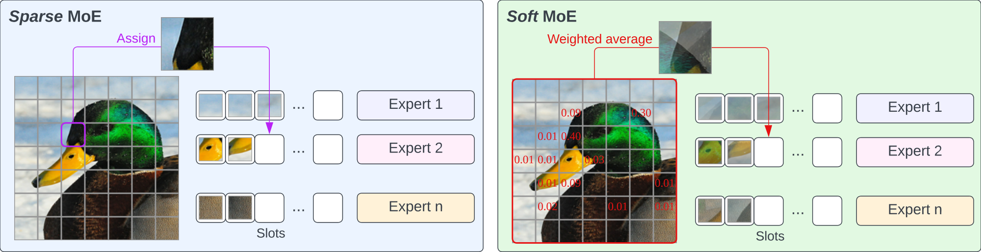
Sparse MoE Transformers involve a discrete optimization problem to decide which modules should be applied to each token. These modules are commonly referred to as experts and are usually MLPs. Many techniques have been devised to find good token-to-expert matches: linear programs ([8]), reinforcement learning ([9]), deterministic fixed rules ([10]), optimal transport ([11]), greedy top- $k$ experts per token ([12]), or greedy top- $k$ tokens per expert ([13]). Often, heuristic auxiliary losses are required to balance utilization of experts and minimize unassigned tokens. These challenges can be greater in out-of-distribution settings: small inference batch sizes, novel inputs, or in transfer learning.
We introduce Soft MoE, that overcomes many of these challenges. Rather than employing a sparse and discrete router that tries to find a good hard assignment between tokens and experts, Soft MoEs instead perform a soft assignment by mixing tokens. In particular, we compute several weighted averages of all tokens—with weights depending on both tokens and experts—and then we process each weighted average by its corresponding expert.
Soft MoE L/16 outperforms ViT H/14 on upstream, few-shot and finetuning while requiring almost half the training time, and being 2 $\times$ faster at inference. Moreover, Soft MoE B/16 matches ViT H/14 on few-shot and finetuning and outperforms it on upstream metrics after a comparable amount of training. Remarkably, Soft MoE B/16 is 5.7 $\times$ faster at inference despite having 5.5 $\times$ the number of parameters of ViT H/14 (see Table 2 and Figure 5 for details). Section 4 demonstrates Soft MoE's potential to extend to other tasks: we train a contrastive model text tower against the frozen vision tower, showing that representations learned via soft routing preserve their benefits for image-text alignment.
2. Soft Mixture of Experts
Section Summary: The Soft Mixture of Experts (MoE) is a technique used in neural networks, like those in language models, to process input data more efficiently by combining multiple specialized "experts" without making hard choices about which parts of the data each expert handles. Instead of assigning individual input tokens to specific experts, as in traditional Sparse MoE, Soft MoE creates virtual slots by taking weighted averages of all tokens, using soft probabilities from a softmax function to blend them smoothly. This approach makes the entire process fully differentiable and easier to train, avoiding the optimization challenges of discrete assignments, and it can replace parts of a model's processing layers to match the computational cost of standard models.
2.1 Algorithm description
The Soft MoE routing algorithm is depicted in Figure 2. We denote the inputs tokens for one sequence by $\mathbf{X} \in \mathbb{R}^{m \times d}$, where $m$ is the number of tokens and $d$ is their dimension. Each MoE layer uses a set of $n$ expert functions[^1] applied on individual tokens, namely ${f_i: \mathbb{R}^d \rightarrow \mathbb{R}^d }_{1:n}$. Each expert processes $p$ slots, and each slot has a corresponding $d$-dimensional vector of parameters, $\mathbf{\Phi} \in \mathbb{R}^{d \times (n \cdot p)}$.
[^1]: In practice, all experts apply the same function with different parameters, usually an MLP.
In particular, the input slots $\tilde{\mathbf{X}} \in \mathbb{R}^{(n \cdot p) \times d}$ are the result of convex combinations of all the $m$ input tokens, $\mathbf{X}$:
$ \begin{gathered} \mathbf{D}{ij} = \frac{\exp((\mathbf{X} \mathbf{\Phi}){ij})}{\sum_{i'=1}^m \exp((\mathbf{X} \mathbf{\Phi})_{i'j})}, \qquad \tilde{\mathbf{X}} = \mathbf{D}^\top \mathbf{X}. \end{gathered}\tag{1} $
Notice that $\mathbf{D}$, which we call the dispatch weights, is simply the result of applying a softmax over the columns of $\mathbf{X} \mathbf{\Phi}$. Then, as mentioned above, the corresponding expert function is applied on each slot (i.e. on rows of $\tilde{\mathbf{X}}$) to obtain the output slots: $\tilde{\mathbf{Y}}i = f{\left\lfloor{i / p}\right\rfloor}(\tilde{\mathbf{X}}_i)$.
Finally, the output tokens $\mathbf{Y}$ are computed as a convex combination of all ($n \cdot p$) output slots, $\tilde{\mathbf{Y}}$, whose weights are computed similarly as before:
$ \begin{gathered} \mathbf{C}{ij} = \frac{\exp((\mathbf{X} \mathbf{\Phi}){ij})}{\sum_{j'=1}^{n \cdot p} \exp((\mathbf{X} \mathbf{\Phi})_{ij'})}, \qquad \mathbf{Y} = \mathbf{C} \tilde{\mathbf{Y}}. \end{gathered}\tag{2} $
We refer to $\mathbf{C}$ as the combine weights, and it is the result of applying a softmax over the rows of $\mathbf{X} \mathbf{\Phi}$.
Following the usual design for Sparse MoEs, we replace a subset of the Transformer's MLP blocks with Soft MoE blocks. We typically replace the second half of MLP blocks. The total number of slots is a key hyperparameter of Soft MoE layers because the time complexity depends on the number of slots rather than on the number of experts. One can set the number of slots equal to the input sequence length to match the FLOPs of the equivalent dense Transformer.
:::: {.figure}
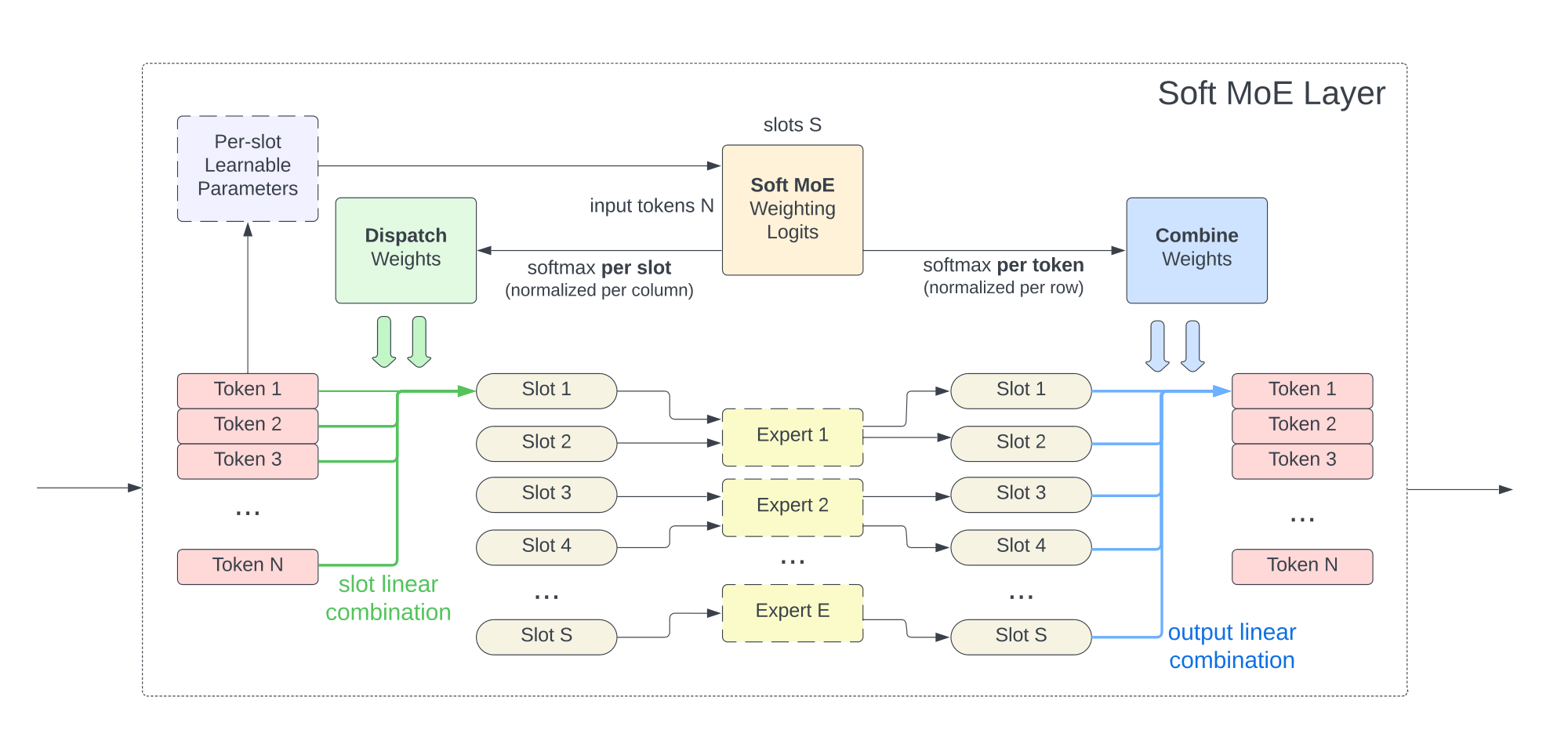 Figure 2: \caption{
Figure 2: Soft MoE routing details. Figure 2: Soft MoE computes scores or logits for every pair of input token and slot.
Figure 2: From this it computes a slots $\times$ tokens matrix of logits, that are normalized appropriately to compute both the dispatch and combine weights.
Figure 2: The slots themselves are allocated to experts round-robin.
Figure 2: : Soft MoE routing details. Figure 2: Soft MoE computes scores or logits for every pair of input token and slot. Figure 2: From this it computes a slots $\times$ tokens matrix of logits, that are normalized appropriately to compute both the dispatch and combine weights. Figure 2: The slots themselves are allocated to experts round-robin.
::::
2.2 Properties of Soft MoE and connections with Sparse MoEs
Fully differentiable
Sparse MoE algorithms involve an assignment problem between tokens and experts, which is subject to capacity and load-balancing constraints. Different algorithms approximate the solution in different ways: for example, the top- $k$ or "Token Choice" router ([12, 4, 6]) selects the top- $k$-scored experts for each token, while there are slots available in such expert (i.e. the expert has not filled its capacity). The "Expert Choice" router ([13]) selects the top-capacity-scored tokens for each expert. Other works suggest more advanced (and often costly) algorithms to compute the assignments, such as approaches based on Linear Programming algorithms ([8]), Optimal Transport ([11, 14]) or Reinforcement Learning ([14]). Nevertheless virtually all of these approaches are discrete in nature, and thus non-differentiable. In contrast, all operations in Soft MoE layers are continuous and fully differentiable. We can interpret the weighted averages with softmax scores as soft assignments, rather than the hard assignments used in Sparse MoE.
(https://github.com/google-research/vmoe).}, label=alg:soft_moe_python, escapechar=|]
def soft_moe_layer(X, Phi, experts):
  # Compute the dispatch and combine weights.
  logits = jnp.einsum('md,dnp->mnp', X, Phi)|\label{line:logits}|
  D = jax.nn.softmax(logits, axis=(0,))
  C = jax.nn.softmax(logits, axis=(1, 2))
  # The input slots are a weighted average of all the input tokens,
  # given by the dispatch weights.
  Xs = jnp.einsum('md,mnp->npd', X, D)
  # Apply the corresponding expert function to each input slot.
  Ys = jnp.stack([
    f_i(Xs[i, :, :]) for i, f_i in enumerate(experts)],
    axis=0)
  # The output tokens are a weighted average of all the output slots,
  # given by the combine weights.
  Y = jnp.einsum('npd,mnp->md', Ys, C)
  return Y
No token dropping and expert unbalance
The classical routing mechanisms tend to suffer from issues such as "token dropping" (i.e. some tokens are not assigned to any expert), or "expert unbalance" (i.e. some experts receive far more tokens than others). Unfortunately, performance can be severely impacted as a consequence. For instance, the popular top- $k$ or "Token Choice" router ([12]) suffers from both, while the "Expert Choice" router ([13]) only suffers from the former (see Appendix B for some experiments regarding dropping). Soft MoEs are immune to token dropping and expert unbalance since every slot is filled with a weighted average of all tokens.
Fast
The total number of slots determines the cost of a Soft MoE layer. Every input applies such number of MLPs. The total number of experts is irrelevant in this calculation: few experts with many slots per expert or many experts with few slots per expert will have matching costs if the total number of slots is identical. The only constraint we must meet is that the number of slots has to be greater or equal to the number of experts (as each expert must process at least one slot). The main advantage of Soft MoE is completely avoiding sort or top- $k$ operations which are slow and typically not well suited for hardware accelerators. As a result, Soft MoE is significantly faster than most sparse MoEs (Figure 6). See Section 2.3 for time complexity details.
Features of both sparse and dense
The sparsity in Sparse MoEs comes from the fact that expert parameters are only applied to a subset of the input tokens. However, Soft MoEs are not technically sparse, since every slot is a weighted average of all the input tokens. Every input token fractionally activates all the model parameters. Likewise, all output tokens are fractionally dependent on all slots (and experts). Finally, notice also that Soft MoEs are not Dense MoEs, where every expert processes all input tokens, since every expert only processes a subset of the slots.
Per-sequence determinism
Under capacity constraints, all Sparse MoE approaches route tokens in groups of a fixed size and enforce (or encourage) balance within the group. When groups contain tokens from different sequences or inputs, these tokens compete for available spots in expert buffers. Therefore, the model is no longer deterministic at the sequence-level, but only at the batch-level. Models using larger groups tend to provide more freedom to the routing algorithm and usually perform better, but their computational cost is also higher.
2.3 Implementation
Time complexity
Assume the per-token cost of a single expert function is $O(k)$. The time complexity of a Soft MoE layer is then $O(mnpd + npk)$. By choosing $p = O({m}/{n})$ slots per expert, i.e. the number of tokens over the number of experts, the cost reduces to $O(m^2 d + m k)$. Given that each expert function has its own set of parameters, increasing the number of experts $n$ and scaling $p$ accordingly, allows us to increase the total number of parameters without any impact on the time complexity. Moreover, when the cost of applying an expert is large, the $mk$ term dominates over $m^2 d$, and the overall cost of a Soft MoE layer becomes comparable to that of applying a single expert on all the input tokens. Finally, even when $m^2 d$ is not dominated, this is the same as the (single-headed) self-attention cost, thus it does not become a bottleneck in Transformer models. This can be seen in the bottom plot of Figure 6 where the throughput of Soft MoE barely changes when the number of experts increases from 8 to 4, 096 experts, while Sparse MoEs take a significant hit.
Normalization
In Transformers, MoE layers are typically used to replace the feedforward layer in each encoder block. Thus, when using pre-normalization as most modern Transformer architectures ([16, 17, 6, 5]), the inputs to the MoE layer are "layer normalized". This causes stability issues when scaling the model dimension $d$, since the softmax approaches a one-hot vector as $d \rightarrow \infty$ (see Appendix E). Thus, in Section 2.2 of [@alg:soft_moe_python] we replace X and Phi with l2_normalize(X, axis=1) and scale * l2_normalize(Phi, axis=0), respectively; where scale is a trainable scalar, and l2_normalize normalizes the corresponding axis to have unit (L2) norm, as Algorithm 1 shows.
def l2_normalize(x, axis, eps=1e-6):
  norm = jnp.sqrt(jnp.square(x).sum(axis=axis, keepdims=True))
  return x * jnp.reciprocal(norm + eps)
For relatively small values of $d$, the normalization has little impact on the model's quality. However, with the proposed normalization in the Soft MoE layer, we can make the model dimension bigger and/or increase the learning rate (see Appendix E).
Distributed model
When the number of experts increases significantly, it is not possible to fit the entire model in memory on a single device, especially during training or when using MoEs on top of large model backbones. In these cases, we employ the standard techniques to distribute the model across many devices, as in ([4, 6, 5]) and other works training large MoE models. Distributing the model typically adds an overhead in the cost of the model, which is not captured by the time complexity analysis based on FLOPs that we derived above. In order to account for this difference, in all of our experiments we measure not only the FLOPs, but also the wall-clock time in TPUv3-chip-hours.
3. Image Classification Experiments
Section Summary: This section describes experiments testing Soft MoE models, a type of efficient neural network, against standard Vision Transformers (ViT) and other sparse models for classifying images. Researchers trained various model sizes on a massive dataset of over 4 billion images and evaluated them using metrics like accuracy on a smaller benchmark called ImageNet, showing that Soft MoE consistently outperforms denser models in terms of performance for the same training time or computing power. They also explored longer training sessions for faster inference, adjusted model components like expert numbers, and tested different ways tokens route through the network to optimize results.
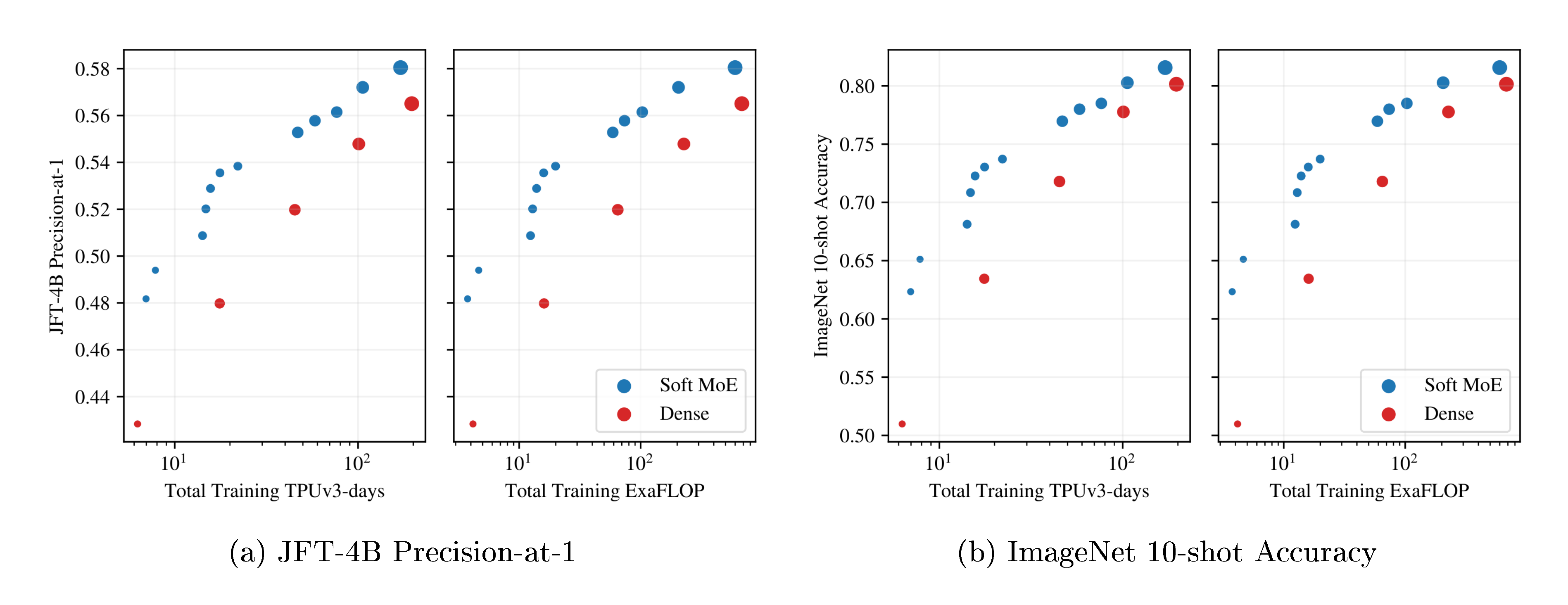
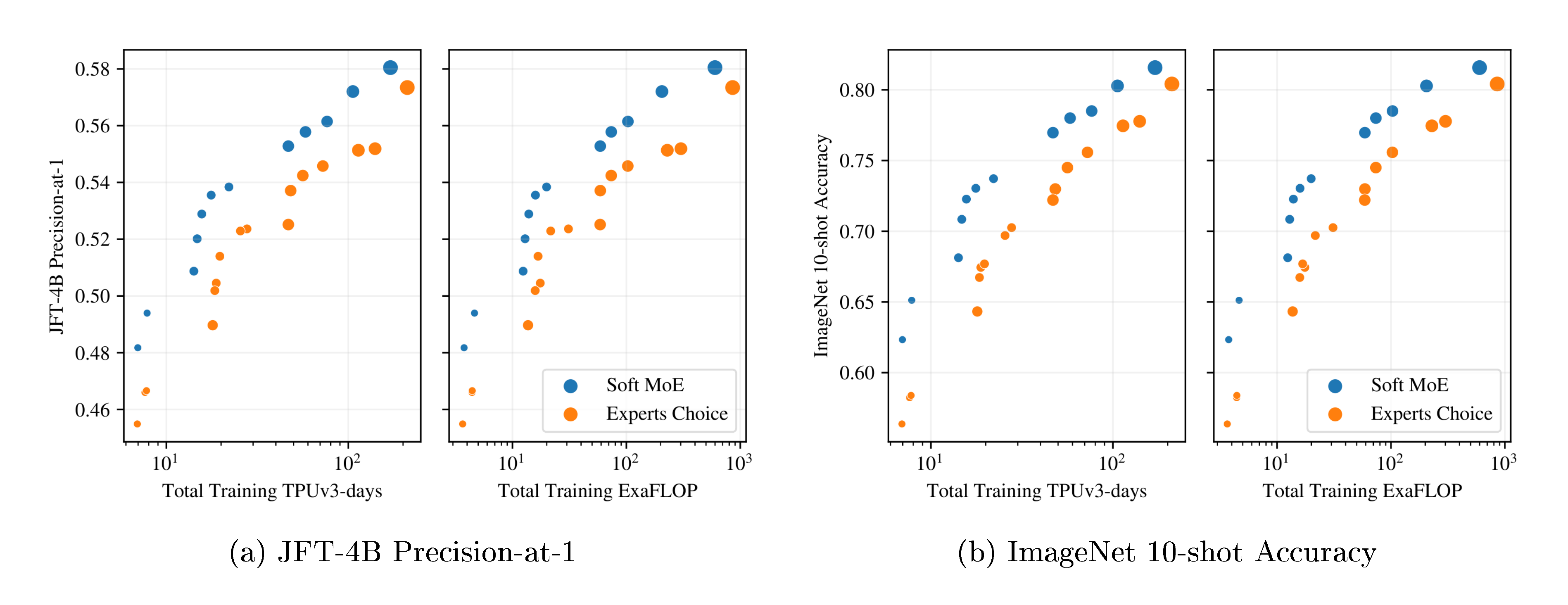
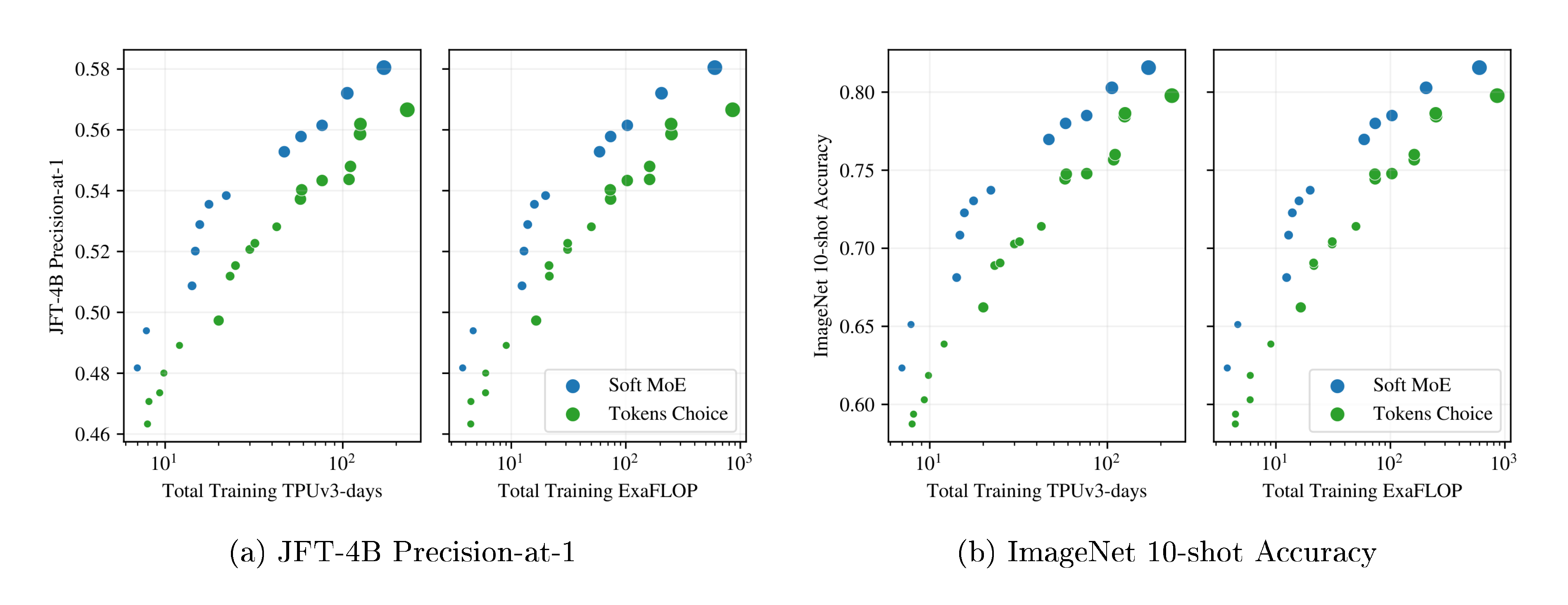
Training Pareto frontiers. In Section 3.3 we compare dense ViT models at the Small, Base, Large and Huge sizes with their dense and sparse counterparts based on both Tokens Choice and Experts Choice sparse routing. We study performance at different training budgets and show that Soft MoE dominates other models in terms of performance at a given training cost or time.
Inference-time optimized models. In Section 3.4, we present longer training runs ("overtraining"). Relative to ViT, Soft MoE brings large improvements in terms of inference speed for a fixed performance level (smaller models: S, B) and absolute performance (larger models: L, H).
Model ablations. In Section 3.5 and Section 3.6 we investigate the effect of changing slot and expert counts, and perform ablations on the Soft MoE routing algorithm.
3.1 Training and evaluation data
We pretrain our models on JFT-4B ([3]), a proprietary dataset that contains more than 4B images, covering 29k classes. During pretraining, we evaluate the models on two metrics: upstream validation precision-at-1 on JFT-4B, and ImageNet 10-shot accuracy. The latter is computed by freezing the model weights and replacing the head with a new one that is only trained on a dataset containing 10 images per class from ImageNet-1k ([18]). Finally, we provide the accuracy on the validation set of ImageNet-1k after finetuning on the training set of ImageNet-1k (1.3 million images) at 384 resolution.
3.2 Sparse routing algorithms
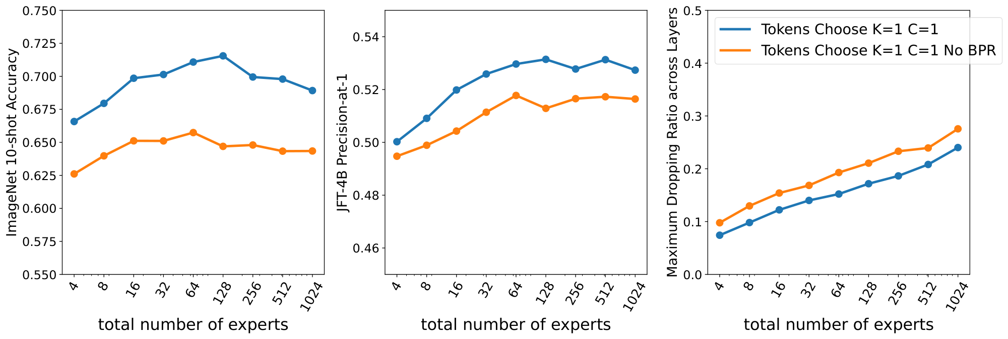
Tokens Choice. Every token selects the top- $K$ experts with the highest routing score for the token ([12]). Increasing $K$ typically leads to better performance at increased computational cost. Batch Priority Routing (BPR) ([6]) significantly improves the model performance, especially in the case of $K=1$ (Appendix F, Table 8). Accordingly we use Top- $K$ routing with BPR and $K \in {1, 2}$. We also optimize the number of experts (Appendix F, Figure 11).
Experts Choice. Alternatively, experts can select the top- $C$ tokens in terms of routing scores ([13]). $C$ is the buffer size, and we set $E \cdot C = c \cdot T$ where $E$ is the number of experts, $T$ is the total number of tokens in the group, and $c$ is the capacity multiplier. When $c = 1$, all tokens can be processed via the union of experts. With Experts Choice routing, it is common that some tokens are simultaneously selected by several experts whereas some other tokens are not selected at all. Figure 10, Appendix B illustrates this phenomenon. We experiment with $c=0.5, 1, 2$.
3.3 Training Pareto-optimal models
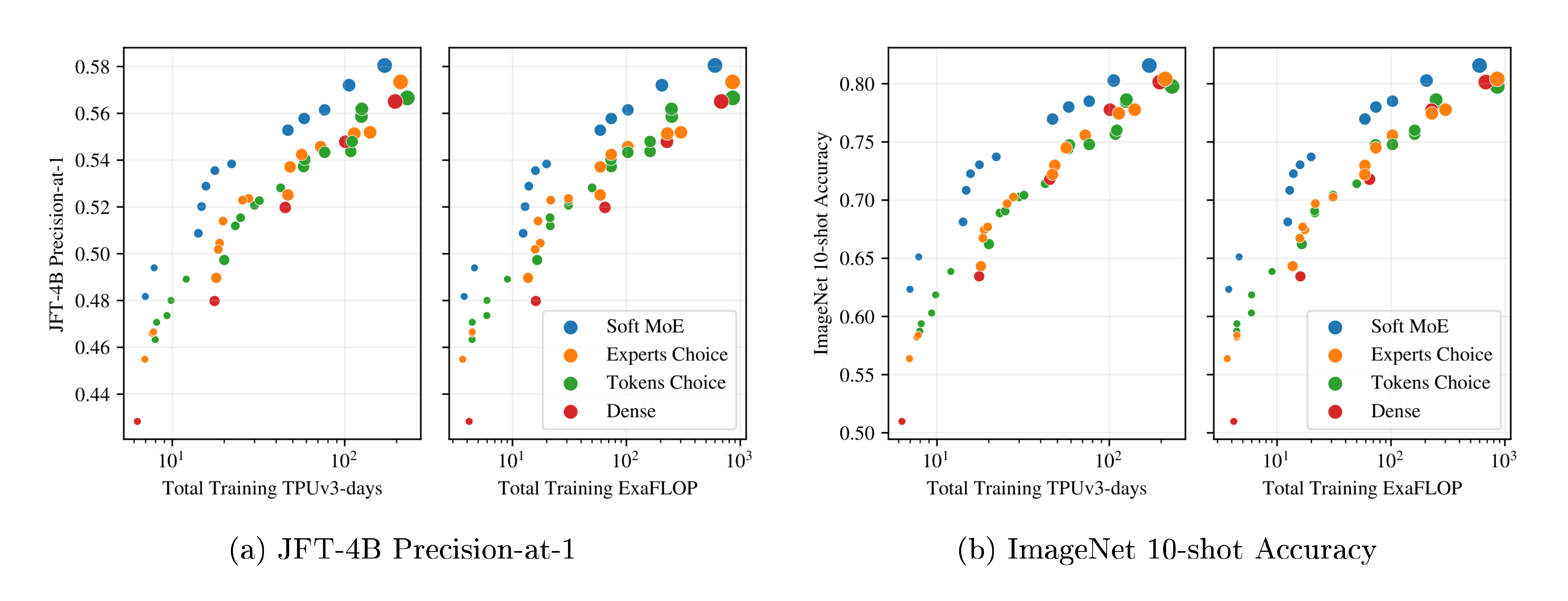
We trained ViT-{S/8, S/16, S/32, B/16, B/32, L/16, L/32, H/14} models and their sparse counterparts. We trained several variants (varying $K$, $C$ and expert number), totalling 106 models. We trained for 300k steps with batch size 4096, resolution 224, using a reciprocal square root learning rate schedule.
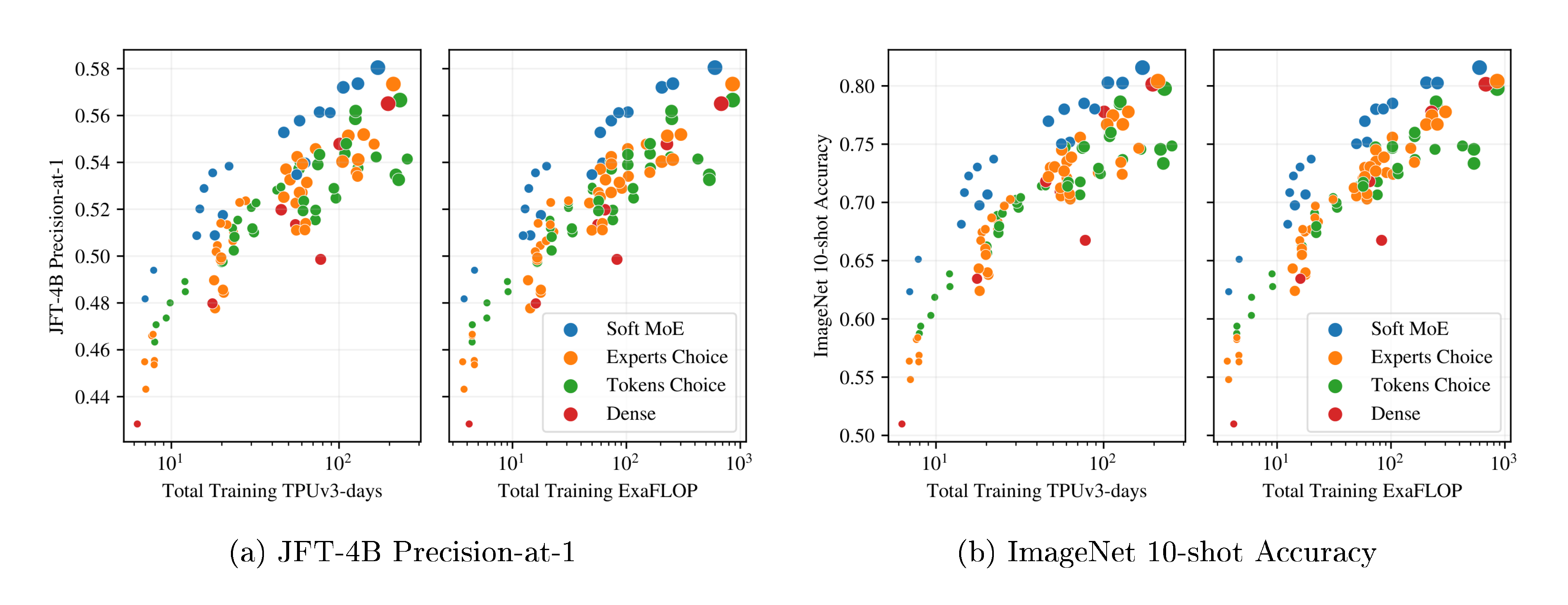
Figure 3a and Figure 3b show the results for models in each class that lie on their respective training cost/performance Pareto frontiers. On both metrics, Soft MoE strongly outperforms dense and other sparse approaches for any given FLOPs or time budget. Table 10, Appendix J, lists all the models, with their parameters, performance and costs, which are all displayed in Figure 19.
3.4 Long training durations
We trained a number of models for much longer durations, up to 4M steps. We trained a number of Soft MoEs on JFT, following a similar setting to [3]. We replace the last half of the blocks in ViT S/16, B/16, L/16, and H/14 with Soft MoE layers with 128 experts, using one slot per expert. We train models ranging from 1B to 54B parameters. All models were trained for 4M steps, except for H/14, which was trained for 2M steps for cost reasons.
::::
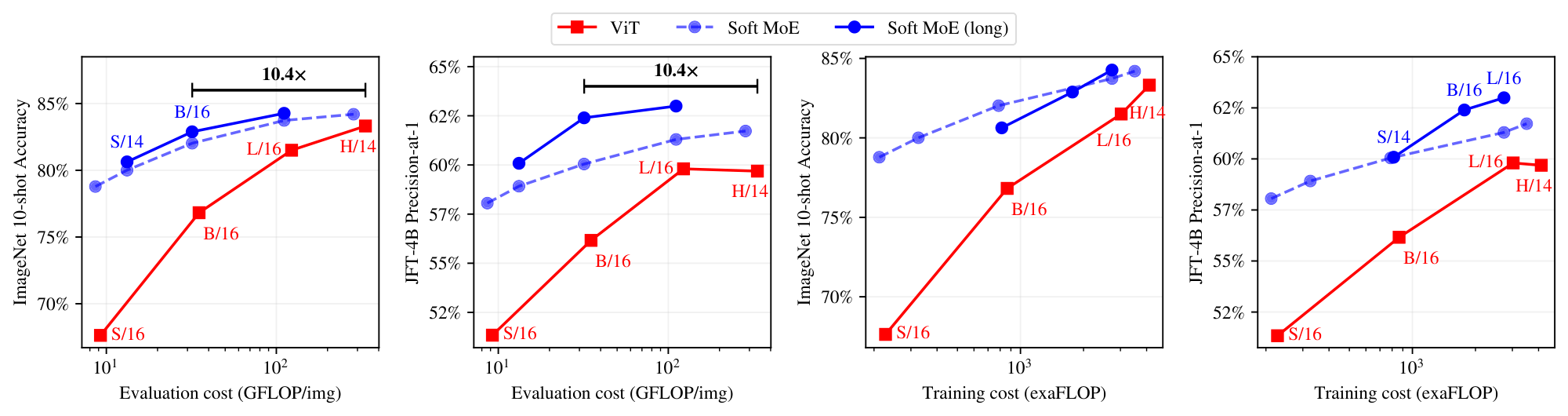
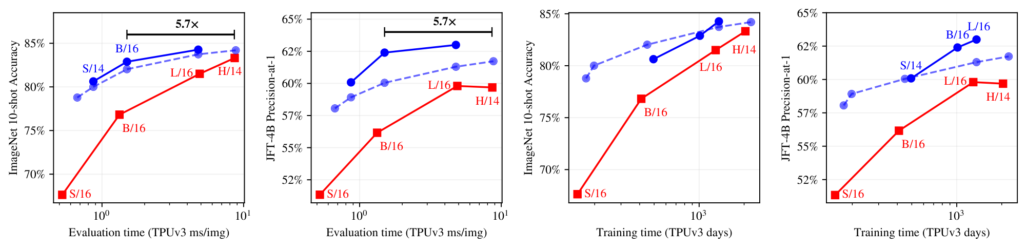
Figure 5: Models optimized for inference speed. Performance of models trained for more steps, thereby optimized for performance at a given inference cost (TPUv3 time or FLOPs). ::::
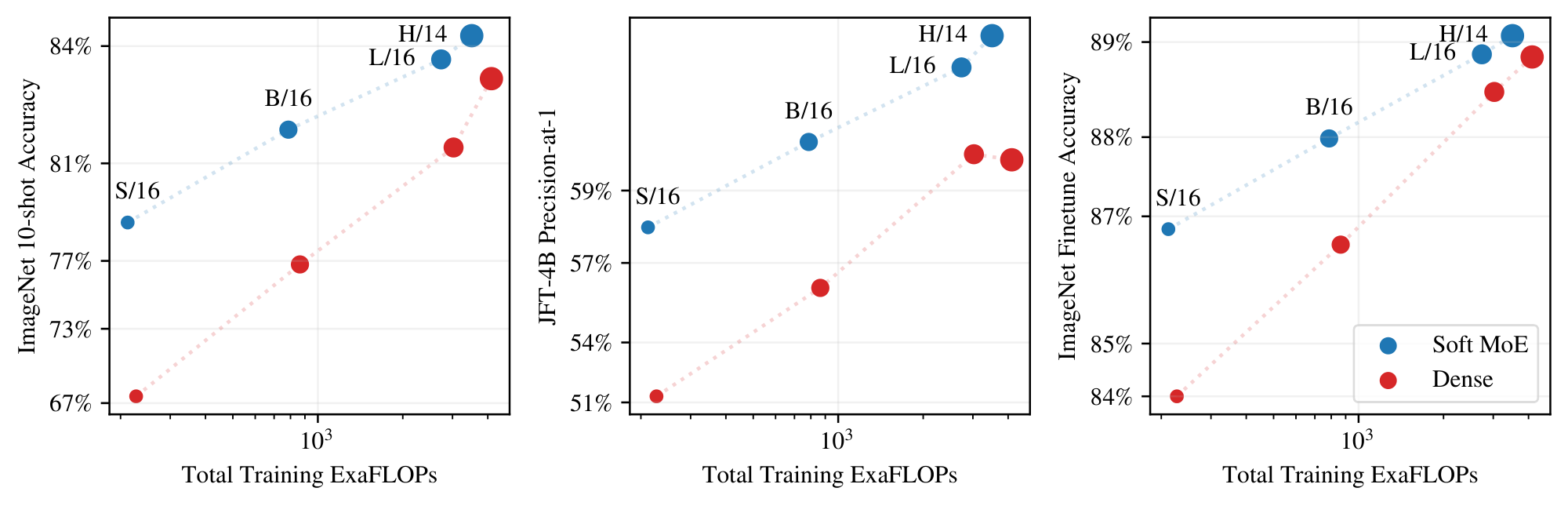
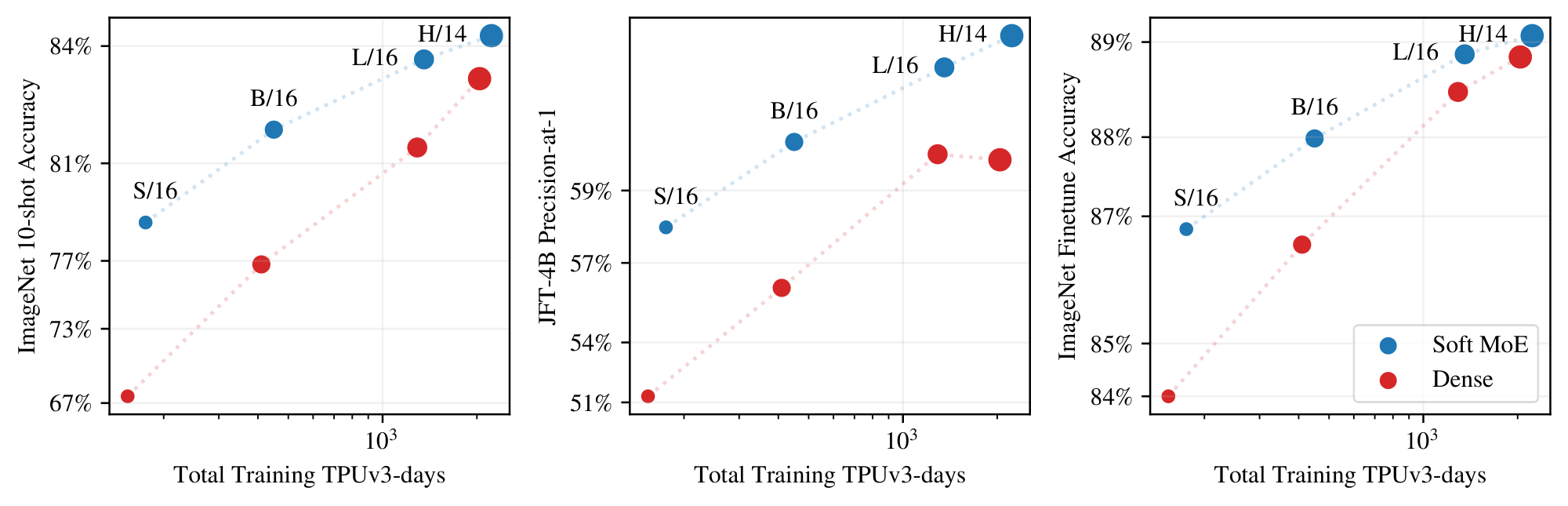
Figure 4 shows the JFT-4B precision, ImageNet 10-shot accuracy, and the ImageNet finetuning accuracy for Soft MoE and ViT versus training cost. Appendix F, Table 9 contains numerical results, and Figure 16 shows performance versus core-hours, from which the same conclusions can be drawn. Soft MoE substantially outperforms dense ViT models for a given compute budget. For example, the Soft MoE S/16 performs better than ViT B/16 on JFT and 10-shot ImageNet, and it also improves finetuning scores on the full ImageNet data, even though its training (and inference) cost is significantly smaller. Similarly, Soft MoE B/16 outperforms ViT L/16 upstream, and only lags 0.5 behind after finetuning while being 3x faster and requiring almost 4x fewer FLOPs. Finally, the Soft MoE L/16 model outperforms the dense H/14 one while again being around 3x faster in terms of training and inference step time.
We continue training the small backbones up to 9M steps to obtain models of high quality with low inference cost. Even after additional (over) training, the overall training time with respect to larger ViT models is similar or smaller. For these runs, longer cooldowns (linear learning rate decay) works well for Soft MoE. Therefore, we increase the cooldown from 50k steps to 500k steps.
Figure 5 and Table 2 present the results. Soft MoE B/16 trained for 1k TPUv3 days matches or outperforms ViT H/14 trained on a similar budget, and is 10 $\times$ cheaper at inference in FLOPs (32 vs. 334 GFLOPS/img) and $\bf >5\times$ cheaper in wall-clock time (1.5 vs. 8.6 ms/img). Soft MoE B/16 matches the ViT H/14 model's performance when we double ViT-H/14's training budget (to 2k TPU-days). Soft MoE L/16 outperforms all ViT models while being almost 2 $\times$ faster at inference than ViT H/14 (4.8 vs. 8.6 ms/img).
\begin{tabular}{lrrrrrrrrr}
\toprule
Model & Params & \multicolumn{1}{c}{Train} & \multicolumn{1}{c}{Train} & \multicolumn{1}{c}{Train} & \multicolumn{1}{c}{Eval} & \multicolumn{1}{c}{Eval} & \multicolumn{1}{c}{JFT @1} & \multicolumn{1}{c}{INet} & \multicolumn{1}{c}{INet} \\
 & & \multicolumn{1}{c}{steps (cd)} & \multicolumn{1}{c}{TPU-days} & \multicolumn{1}{c}{exaFLOP} & \multicolumn{1}{c}{ms/img} & \multicolumn{1}{c}{GFLOP/img} & \multicolumn{1}{c}{P@1} & \multicolumn{1}{c}{10shot} & \multicolumn{1}{c}{finetune} \\
\midrule
ViT S/16 & 33M & 4M (50k) & 153.5 & 227.1 & 0.5 & 9.2 & 51.3 & 67.6 & 84.0 \\
ViT B/16 & 108M & 4M (50k) & 410.1 & 864.1 & 1.3 & 35.1 & 56.2 & 76.8 & 86.6 \\
ViT L/16 & 333M & 4M (50k) & 1290.1 & 3025.4 & 4.9 & 122.9 & 59.8 & 81.5 & 88.5 \\
ViT H/14 & 669M & 1M (50k) & 1019.9 & 2060.2 & 8.6 & 334.2 & 58.8 & 82.7 & 88.6 \\
ViT H/14 & 669M & 2M (50k) & 2039.8 & 4120.3 & 8.6 & 334.2 & 59.7 & 83.3 & 88.9 \\
\midrule
\mbox{Soft MoE} S/14 256E & 1.8B & 10M (50k) & 494.7 & 814.2 & 0.9 & 13.2 & 60.1 & 80.6 & 87.5 \\
\mbox{Soft MoE} B/16 128E & 3.7B & 9M (500k) & 1011.4 & 1769.5 & 1.5 & 32.0 & 62.4 & 82.9 & 88.5 \\
\mbox{Soft MoE} L/16 128E & 13.1B & 4M (500k) & 1355.4 & 2734.1 & 4.8 & 111.1 & 63.0 & 84.3 & 89.2 \\
\bottomrule
\end{tabular}
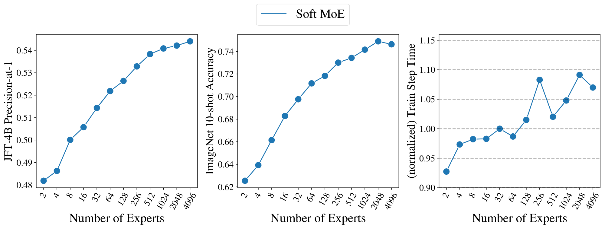
3.5 Number of slots and experts
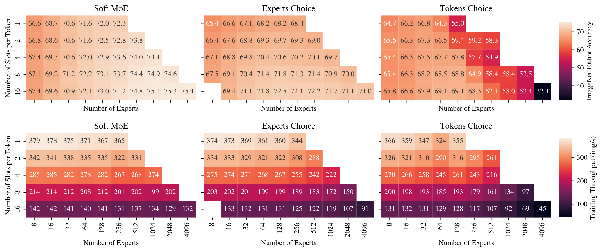
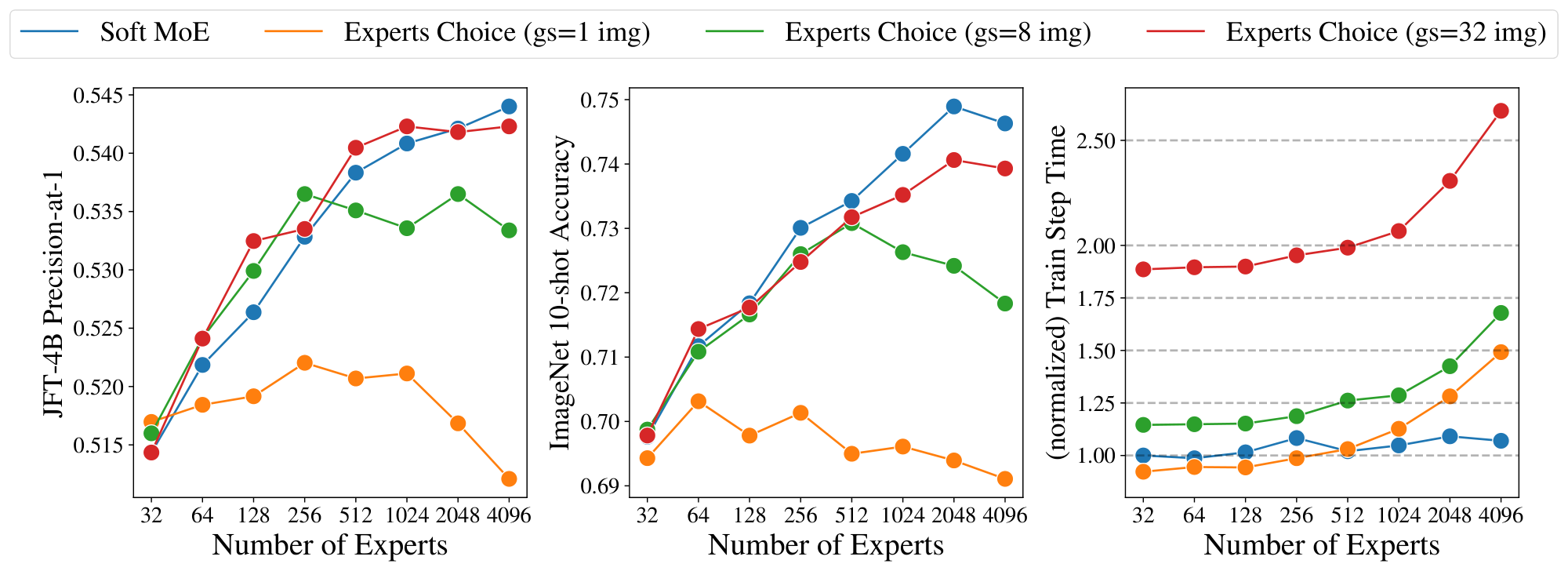
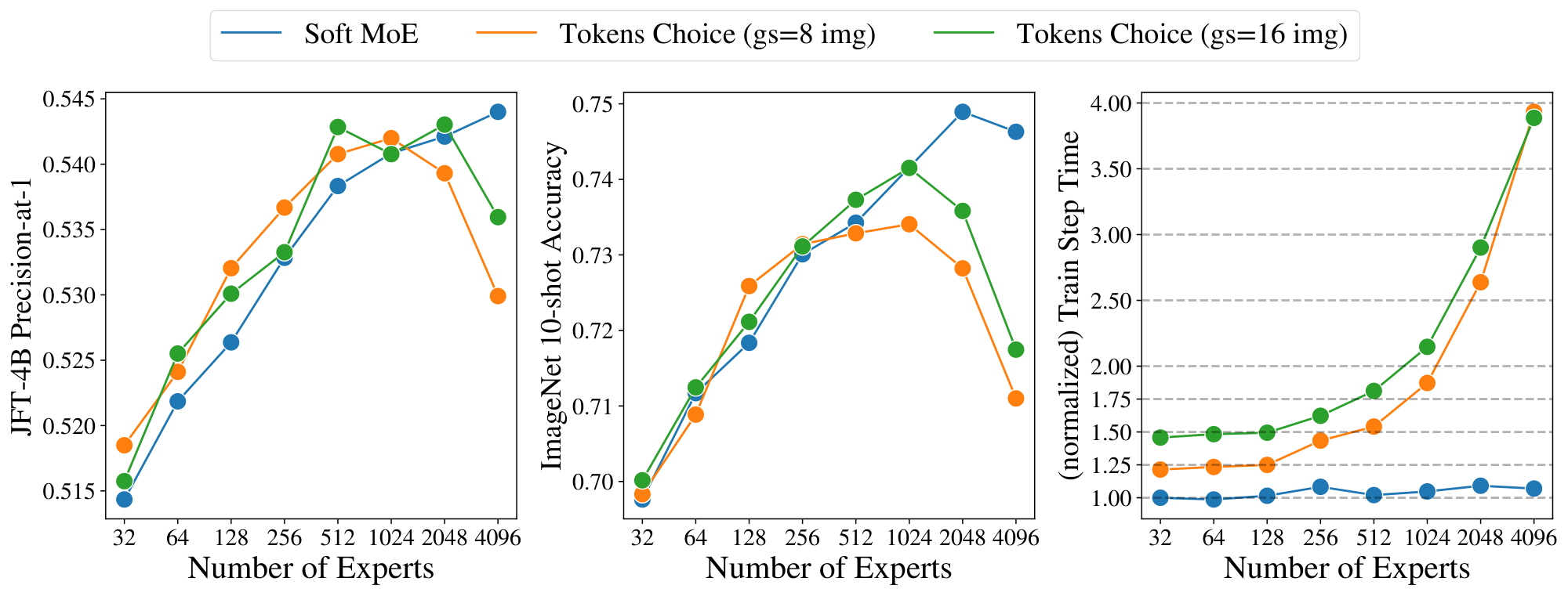
We study the effect of changing the number of slots and experts in the Sparse and Soft MoEs. Figure 6 shows the quality and speed of MoEs with different numbers of experts, and numbers of slots per token; the latter is equivalent to the average number of experts assigned per token for Sparse MoEs. When varying the number of experts, the models' backbone FLOPs remain constant, so changes in speed are due to routing costs. When varying the slots-per-expert, the number of tokens processed in the expert layers increases, so the throughput decreases. First, observe that for Soft MoE, the best performing model at each number of slots-per-token is the model with the most experts (i.e. one slot per expert). For the two Sparse MoEs, there is a point at which training difficulties outweigh the benefits of additional capacity, resulting in the a modest optimum number of experts. Second, Soft MoE's throughput is approximately constant when adding more experts. However, the Sparse MoEs' throughputs reduce dramatically from 1k experts, see discussion in Section 2.2.
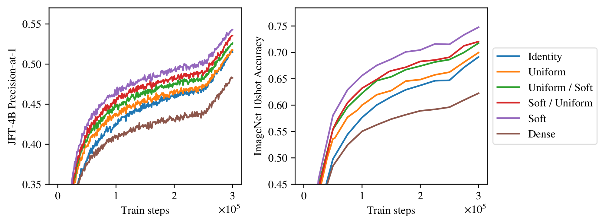
3.6 Ablations
We study the impact of the components of the Soft MoE routing layer by running the following ablations: Identity routing: Tokens are not mixed: the first token goes to first expert, the second token goes to second expert, etc. Uniform Mixing: Every slot mixes all input tokens in the same way: by averaging them, both for dispatching and combining. Expert diversity arises from different initializations of their weights. Soft / Uniform: We learn token mixing on input to the experts to create the slots (dispatch weights), but we average the expert outputs. This implies every input token is identically updated before the residual connection. Uniform / Soft. All slots are filled with a uniform average of the input tokens. We learn slot mixing of the expert output tokens depending on the input tokens. Table 3 shows that having slots is important; Identity and Uniform routing substantially underperform Soft MoE, although they do outperform ViT. Dispatch mixing appears slightly more important than the combine mixing. See Appendix A for additional details.
:Table 3: Ablations using Soft MoE-S/14 with 256 experts trained for 300k steps.
| Method | Experts | Mixing | Learned Dispatch | Learned Combine | JFT p@1 | IN/10shot |
|---|---|---|---|---|---|---|
| Soft MoE | \checkmark | \checkmark | \checkmark | \checkmark | 54.3% | 74.8% |
| Soft / Uniform | \checkmark | \checkmark | \checkmark | 53.6% | 72.0% | |
| Uniform / Soft | \checkmark | \checkmark | \checkmark | 52.6% | 71.8% | |
| Uniform | \checkmark | \checkmark | 51.8% | 70.0% | ||
| Identity | \checkmark | 51.5% | 69.1% | |||
| ViT | 48.3% | 62.3% |
4. Contrastive learning
Section Summary: Researchers tested whether the Soft MoE model's image representations work well for linking images with text descriptions through contrastive learning, where the image part of the model is fixed after initial training on a large classification dataset, and a new text component learns from billions of image-text pairs. The results showed that Soft MoE generally outperformed standard models in zero-shot tasks on datasets like ImageNet and Cifar-100, with gains of over 1-2%, though improvements were smaller for retrieval tasks like COCO due to differences in training data. When trained from scratch on a public dataset, Soft MoE also did better than alternatives and made effective use of extra data enhancements.
We test whether the Soft MoE's representations are better for other tasks. For this, we try image-text contrastive learning. Following [19], the image tower is pre-trained on image classification, and then frozen while training the text encoder on a dataset of image-text pairs. We re-use the models trained on JFT in the previous section and compare their performance zero-shot on downstream datasets. For contrastive learning we train on WebLI ([20]), a proprietary dataset consisting of 10B images and alt-texts. The image encoder is frozen, while the text encoder is trained from scratch.
Table 4 shows the results. Overall, the benefits we observed on image classification are also in this setting. For instance, Soft MoE -L/16 outperforms ViT-L/16 by more than 1% and 2% on ImageNet and Cifar-100 zero-shot, respectively. However, the improvement on COCO retrieval are modest, and likely reflects the poor alignment between features learned on closed-vocabulary JFT and this open-vocabulary task.
\begin{tabular}{lrrrrrr}
\toprule
Model & Experts & IN/0shot & Cifar100/0shot & Pet/0shot & Coco Img2Text & Coco Text2Img \\
\midrule
ViT-S/16 & -- & 74.2\% & 56.6\% & 94.8\% & 53.6\% & 37.0\% \\
\mbox{Soft MoE}-S/16 & 128 & 81.2\% & 67.2\% & 96.6\% & 56.0\% & 39.0\% \\
\mbox{Soft MoE}-S/14 & 256 & 82.0\% & 75.1\% & 97.1\% & 56.5\% & 39.4\% \\
\midrule
ViT-B/16 & -- & 79.6\% & 71.0\% & 96.4\% & 58.2\% & 41.5\% \\
\mbox{Soft MoE}-B/16 & 128 & 82.5\% & 74.4\% & 97.6\% & 58.3\% & 41.6\% \\
\midrule
ViT-L/16 & -- & 82.7\% & 77.5\% & 97.1\% & 60.7\% & 43.3\% \\
\mbox{Soft MoE}-L/16 & 128 & 83.8\% & 79.9\% & 97.3\% & 60.9\% & 43.4\% \\
Souped \mbox{Soft MoE}-L/16 & 128 & 84.3\% & 81.3\% & 97.2\% & 61.1\% & 44.5\% \\
\midrule
ViT-H/14 & -- & 83.8\% & 84.7\% & 97.5\% & 62.7\% & 45.2\% \\
\mbox{Soft MoE}-H/14 & 256 & 84.6\% & 86.3\% & 97.4\% & 61.0\% & 44.8\% \\
\bottomrule
\end{tabular}
Finally, in Appendix F.1 we show that Soft MoE s also surpass vanilla ViT and the Experts Choice router when trained from scratch on the publicly available LAION-400M ([21]). With this pretraining, Soft MoE s also benefit from data augmentation, but neither ViT nor Experts Choice seem to benefit from it, which is consistent with our observation in Section 3.5, that Soft MoE s make a better use of additional expert parameters.
5. Related Work
Section Summary: Existing research often combines or shortens input sequences in AI models by merging tokens through weighted averages similar to attention mechanisms, aiming to cut down on the heavy computational load of processing long sequences. In contrast, the Soft MoE approach calculates these weights in a comparable way but focuses on blending expert model outputs without shrinking the sequence length, ultimately restoring the full original size after each layer. While multi-headed attention shares some traits with Soft MoE, such as treating heads as simple linear experts that get weighted and combined, Soft MoE uses more complex non-linear experts that handle the entire data dimension from start to finish; other mixture-of-experts methods blend the experts' internal parameters instead of routing data to them, which keeps things fully trainable but ramps up costs due to parameter averaging and limited efficiency in processing varied inputs.
Many existing works merge, mix or fuse input tokens to reduce the input sequence length ([22, 23, 24, 25]), typically using attention-like weighted averages with fixed keys, to try to alleviate the quadratic cost of self-attention with respect to the sequence length. Although our dispatch and combine weights are computed in a similar fashion to these approaches, our goal is not to reduce the sequence length (while it is possible), and we actually recover the original sequence length after weighting the experts' outputs with the combine weights, at the end of each Soft MoE layer.
Multi-headed attention also shows some similarities with Soft MoE, beyond the use of softmax in weighted averages: the $h$ different heads can be interpreted as different (linear) experts. The distinction is that, if $m$ is the sequence length and each input token has dimensionality $d$, each of the $h$ heads processes $m$ vectors of size ${d}/{h}$. The $m$ resulting vectors are combined using different weights for each of the $m'$ output tokens (i.e. the attention weights), on each head independently, and then the resulting $(d/h)$-dimensional vectors from each head are concatenated into one of dimension $d$. Our experts are non-linear and combine vectors of size $d$, at the input and output of such experts.
Other MoE works use a weighted combination of the experts parameters, rather than doing a sparse routing of the examples ([26, 27, 28]). These approaches are also fully differentiable, but they can have a higher cost, since 1) they must average the parameters of the experts, which can become a time and/or memory bottleneck when experts with many parameters are used; and 2) they cannot take advantage of vectorized operations as broadly as Soft (and Sparse) MoEs, since every input uses a different weighted combination of the parameters. We recommend the "computational cost" discussion in [28].
6. Current limitations
Section Summary: Soft MoE has trouble working in auto-regressive decoders, which generate text step by step while keeping past information separate from future predictions, because the method relies on mixing all input tokens together and could accidentally create unwanted biases in how experts process them; researchers see potential here but plan to explore it later. Another issue is that Soft MoE performs best with one slot per expert rather than sharing slots, as combined slots don't add much value and experts struggle with diverse inputs, leading to the need for many experts that inflate the model's memory use even if the overall computing cost stays similar to simpler models.
Auto-regressive decoding
One of the key aspects of Soft MoE consists in learning the merging of all tokens in the input. This makes the use of Soft MoEs in auto-regressive decoders difficult, since causality between past and future tokens has to be preserved during training. Although causal masks used in attention layers could be used, one must be careful to not introduce any correlation between token and slot indices, since this may bias which token indices each expert is trained on. The use of Soft MoE in auto-regressive decoders is a promising research avenue that we leave for future work.
Lazy experts & memory consumption
We show in Section 3 that one slot per expert tends to be the optimal choice. In other words, rather than feeding one expert with two slots, it is more effective to use two experts with one slot each. We hypothesize slots that use the same expert tend to align and provide small informational gains, and a expert may lack the flexibility to accommodate very different slot projections. We show this in Appendix I. Consequently, Soft MoE can leverage a large number of experts and—while its cost is still similar to the dense backbone—the memory requirements of the model can grow large.
Appendix
Section Summary: The appendix compares Soft MoE, a flexible method for assigning data to specialized model components called experts, against simpler fixed routing strategies like Identity (which assigns tokens in order) and Uniform (which averages all tokens evenly). These alternatives underperform Soft MoE significantly in experiments on image models, as shown in figures and tables. It also examines token dropping in two expert selection approaches—Experts Choose and Tokens Choose—finding that dropping rates rise with more experts, though adding slight buffer capacity or smart dropping rules can reduce it and boost performance without much extra cost.
A. Soft vs. Uniform vs. Identity dispatch and combine weights
In this section, we compare Soft MoE (i.e. the algorithm that uses the dispatch and combine weights computed by Soft MoE in Equation 1 and 2) with different "fixed routing" alternatives, where neither the expert selected nor the weight of the convex combinations depend on the content of the tokens.
We consider the following simple modifications of Soft MoE:
Identity. The first token in the sequence is processed by the first expert, the second token by the second expert, and so on in a round robin fashion. When the sequence length is the same as the number of slots and experts, this is equivalent to replacing the matrix $\mathbf{D}$ in Equation 1 (resp. $\mathbf{C}$ in Equation 2) with an identity matrix.
Uniform. Every input slot is filled with a uniform average of all input tokens, and every output token is a uniform average of all output slots. This is equivalent to replacing the matrix $\mathbf{D}$ from Equation 1 with values $\frac{1}{m}$ in all elements, and a matrix $\mathbf{C}$ from Equation 2 with values $\frac{1}{n p}$ in all elements. We randomly and independently initialize every expert.
Uniform / Soft. Every input slot is filled with a uniform average of all input tokens, but we keep the definition of $\mathbf{C}$ from Equation 2.
Soft / Uniform. Every output token is a uniform average of all output slots, but we keep the definition of $\mathbf{D}$ in Equation 1.
Figure 7 and Table 3 shows the results from this experiment, training a S/14 backbone model with MoEs on the last 6 layers. Since the sequence length is 256, we choose 256 experts and slots (i.e. 1 slot per expert), so that the matrices $\mathbf{D}$ and $\mathbf{C}$ are squared. As shown in the figure, Soft MoE is far better than all the other alternatives. For context, we also add the dense ViT S/14 to the comparison.
B. Token Dropping
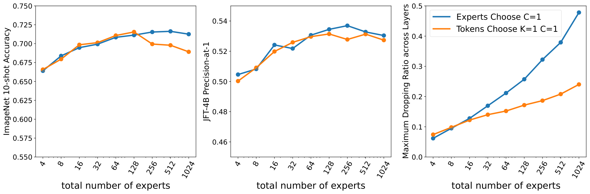
In this appendix, we briefly explore token dropping for the Experts Choose and Tokens Choose algorithms. For Tokens Choose, each token selects $K$ experts. When experts are full, some tokens assigned to that expert will not be processed. A token is "dropped" when none of its choices go through, and no expert at all processes the token. Expert Choose algorithms lead to an uneven amount of processing per token: some input tokens are selected by many experts, while some others are not selected by any. We usually define the number of tokens to be processed by each expert in a way that the combined capacity of all experts corresponds to the number of input tokens (or a multiple $C$ of them). If we use a multiplier $C$ higher than one (say, 2x or 3x), the amount of dropping will decrease but we will pay an increased computational cost. Thus, we mainly explore the $K=1$ and $C=1$ setup, where there is no slack in the buffers.
In all cases to follow we see a common trend: fixing everything constant, increasing the number of experts leads to more and more dropping both in Experts Choose and Tokens Choose.
Figure 8 compares Experts Choose and Tokens Choose with the same multiplier $C=1$. This is the cheapest setup where every token could be assigned to an expert with balanced routing. We see that in both cases the amount of dropping quickly grows with the number of experts. Moreover, even though Experts Choose has higher levels of dropping (especially for large number of experts), it is still more performant than Tokens Choose. Note there is a fundamental difference: when Tokens Choose drops a token, the model wastes that amount of potential compute. On the other hand, for Experts Choose dropping just means some other token got that spot in the expert buffer, thus the model just transferred compute from one unlucky token to another lucky one.
In this setup, for a small number of experts (16-32) it is common to observe a $\sim15%$ rate of dropping. On the other hand, we also experimented with a large number of experts (100-1000) where each expert selects very few tokens. In this case, the dropping rate for Experts Choose can grow above 40-50% in some layers: most experts select the very same tokens. Tokens Choose seems to completely drop up to $\sim$ 25% of the tokens.
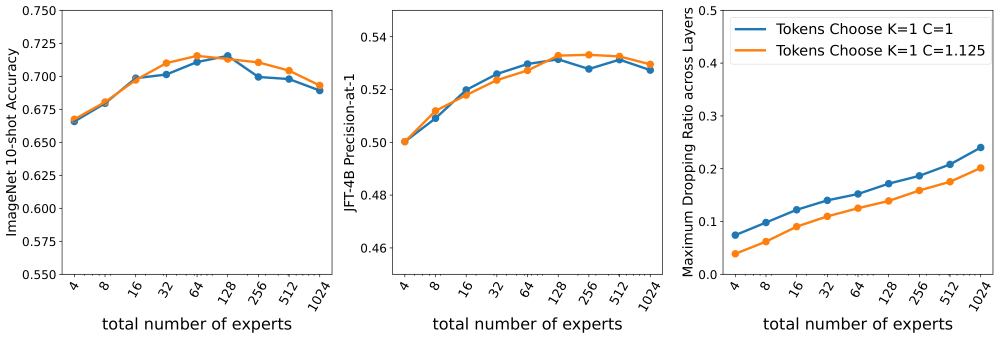
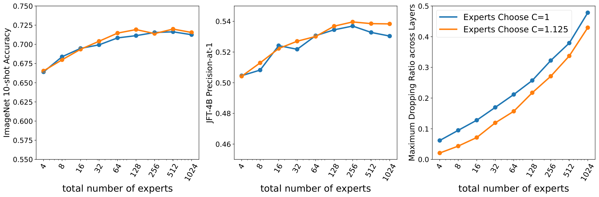
In Figure 10 and Figure 9 we study how much a little bit of buffer slack ($C=1.125$) can help in terms of performance and dropping to Experts Choose and Tokens Choose, respectively. Both plots are similar: the amount of dropping goes down around $\sim$ 5% and performance slightly increases when the number of experts is large. Note that the step time also increases in these cases.
Finally, Figure 11 shows the effect of Batch Priority Routing ([6]) for Tokens Choose. By smartly selecting which tokens to drop we do not only uniformly reduce the amount of dropping, but we significantly bump up performance.
C. Soft MoE Increasing Slots
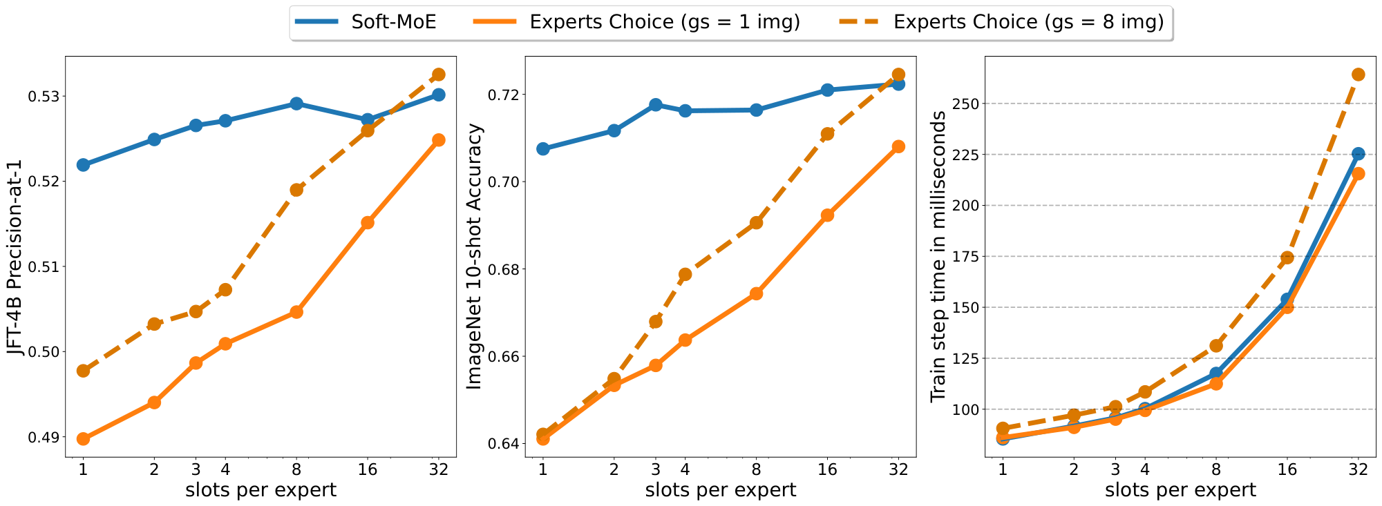
In this section we explore the following question: for a fixed number of experts, how much does Soft MoE routing benefit from having additional slots per expert? Figure 12 shows results for Soft MoE S/16 with 32 experts. We also show Experts Choice with group sizes of one and eight images. When increasing the number of slots, the performance grows only modestly, while cost increases quickly. Experts Choice benefits much more from increased slots, catching up at a large group size, but at a very large cost.
D. Sparse Layers Placement
Soft MoE does unlock the effective use of a large number of experts. An important design choice for sparse models is the number and location of sparse layers, together with the number of experts per layer. Unfortunately, the large number of degrees of freedom in these choices has usually made thorough ablations and optimization unfeasible. In this section, we provide the results of a simple experiment that can help better design the configuration of sparse models. We fix a total number of experts ($E=512$) with one slot per expert, thus leading to matched number of parameters (note in this case FLOPs may vary greatly depending on the number of sparse layers). Then, for an S/16 backbone architecture, we distribute those experts in various ways (all in one layer, half of them in two layers, etc) and compare their performance after 300k training steps. Table 5 shows the results. Again, we observe that a number of experts close to the number of input tokens (there are 196 tokens, given the 16x16 patch size for 224x224 images) split over the last few layers works best. Moreover, note these models are indeed cheaper than those in the comparison with 512 or 256 experts per layer. Table 6 offers results for Tokens Choose routing with $K=1$ and BPR [6]. In this case, all algorithms use a comparable FLOPs count (ignoring slightly increasing routing costs with more experts). Results are essentially similar, thus suggesting optimal expert placement (including expert count and location) may not strongly depend on the routing algorithm.
\begin{tabular}{ ccccccc }
\toprule
Sparse Layers & Experts per Layer & Total Experts & IN/10shot & JFT prec\@1 \\
\midrule
11 & 512 & 512 & 70.0\% & 51.5\% \\
10 & 512 & 512 & 70.1\% & 52.0\% \\
\midrule
10, 11 & 256 & 512 & 71.7\% & 52.2\% \\
5, 11 & 256 & 512 & 70.4\% & 52.1\% \\
\midrule
8, 9, 10, 11 & 128 & 512 & \textbf{72.8\%} & \textbf{53.2\%} \\
2, 5, 8, 11 & 128 & 512 & 71.1\% & 52.5\% \\
\midrule
4:11 & 64 & 512 & \textbf{72.1\%} & \textbf{53.1\%} \\
1:4, 8:11 & 64 & 512 & 70.5\% & 52.1\% \\
\bottomrule
\end{tabular}
\begin{tabular}{ ccccccc }
\toprule
Sparse Layers & Experts per Layer & Total Experts & IN/10shot & JFT prec\@1 \\
\midrule
11 & 512 & 512 & 64.4\% & 50.1\% \\
10 & 512 & 512 & 67.2\% & 51.9\% \\
\midrule
10, 11 & 256 & 512 & 68.6\% & 51.3\% \\
5, 11 & 256 & 512 & 65.3\% & 50.6\% \\
\midrule
8, 9, 10, 11 & 128 & 512 & \textbf{69.1\%} & \textbf{52.3\%} \\
2, 5, 8, 11 & 128 & 512 & 67.3\% & 51.1\% \\
\midrule
4:11 & 64 & 512 & \textbf{69.9\%} & \textbf{52.2\%} \\
1:4, 8:11 & 64 & 512 & 68.0\% & 51.2\% \\
\bottomrule
\end{tabular}
\begin{tabular}{ ccccccc }
\toprule
Sparse Layers & Experts per Layer & Total Experts & IN/10shot & JFT prec\@1 \\
\midrule
11 & 512 & 512 & 65.3\% & 50.3\% \\
10 & 512 & 512 & 66.5\% & 51.7\% \\
\midrule
10, 11 & 256 & 512 & 68.8\% & 51.8\% \\
5, 11 & 256 & 512 & 65.9\% & 51.1\% \\
\midrule
8, 9, 10, 11 & 128 & 512 & \textbf{69.4\%} & \textbf{52.2\%} \\
2, 5, 8, 11 & 128 & 512 & 68.0\% & 51.7\% \\
\midrule
4:11 & 64 & 512 & \textbf{69.0\%} & \textbf{52.2\%} \\
1:4, 8:11 & 64 & 512 & 67.4\% & 51.1\% \\
\bottomrule
\end{tabular}
E. The collapse of softmax layers applied after layer normalization
E.1 Theoretical analysis
A softmax layer with parameters $\Theta \in \mathbb{R}^{n \times d}$ transforms a vector $x \in R^d$ into the vector $\text{softmax}(\Theta x) \in \mathbb{R}^n$, with elements:
$ \text{softmax}(\Theta x)i = \frac{\exp((\Theta x)i)}{\sum{j=1}^n \exp((\Theta x)j)} = \frac{\exp(\sum{k=1}^d \theta{ik}x_k) }{\sum_{j=1}^n \exp(\sum_{k=1}^d \theta_{jk}x_k)} $
Layer normalization applies the following operation on $x \in \mathbb{R}^d$.
$ \text{LN}(x)i = \alpha_i \frac{x_i - \mu(x)}{\sigma(x)} + \beta_i; ; \text{ where } ~ \mu(x) = \frac{1}{d} \sum{i=1}^d x_i ~ \text{ and } ~ \sigma(x) = \sqrt{\frac{1}{d} \sum_{i=1}^d (x_i - \mu(x_i))^2} $
Notice that $\text{LN}(x) = \text{LN}(x - \mu(x))$, thus we can rewrite LayerNorm with respect to the centered vector $\tilde{x} = x - \mu(x)$, and the centered vector scaled to have unit norm $\hat{x}_i = \frac{\tilde{x}_i}{|\tilde{x}|}$:
$ \text{LN}(\tilde{x})_i = \alpha_i \frac{\tilde{x}i}{\sqrt{\frac{1}{d} \sum{j=1}^{d} \tilde{x}_j^2}} + \beta_i = \sqrt{d} \alpha_i \frac{\tilde{x}_i}{|\tilde{x}|} + \beta_i = \sqrt{d} \alpha_i \hat{x}_i + \beta_i $
When a softmax layer is applied to the outputs of layer normalization, the outputs of the softmax are given by the equation:
$ \text{softmax}(\Theta \text{LN}(x))i = \frac{\exp(\sum{k=1}^d \theta_{ik}(\sqrt{d} \alpha_k \hat{x}k + \beta_k)) }{\sum{j=1}^n \exp(\sum_{k=1}^d \theta_{jk}(\sqrt{d} \alpha_k \hat{x}_k + \beta_k))} $
By setting $\vartheta_{i} = \sum_{k=1}^d \theta_{ik} \alpha_k \hat{x}k$, and $\delta_i = \sum{k=1}^d \theta_{ik} \beta_k$, the previous equation can be rewritten as:
$ \text{softmax}(\Theta \text{LN}(x))i = \frac{\exp(\sqrt{d} \vartheta_i + \delta_i) }{\sum{j=1}^n \exp(\sqrt{d} \vartheta_j + \delta_j)} $
Define $m = \max_{i \in [n]} \sqrt{d} \vartheta_i - \delta_i$, $M = {i \in [n] : \sqrt{d} \vartheta_i - \delta_i = m}$. Then, the following equality holds:
$ \text{softmax}(\Theta \text{LN}(x))i = \frac{\exp(\sqrt{d} \vartheta_i + \delta_i - m) }{\sum{j=1}^n \exp(\sqrt{d} \vartheta_j + \delta_j - m)} $
Given that $\lim_{d\rightarrow \infty} \exp(\sqrt{d} \vartheta_i + \delta_i - m) = \begin{cases}1 : i \in M\ 0 : i \notin M\end{cases}$ the output of the softmax tends to:
$ \lim_{d \rightarrow \infty} \text{softmax}(\Theta \text{LN}(x))_i = \begin{cases} \frac{1}{|M|} & i \in M\ 0 & i \notin M \end{cases} $
In particular, when the maximum is only achieved by one of the components (i.e. $|M| = 1$), the softmax collapses to a one-hot vector (a vector with all elements equal to 0 except for one).
E.2 Empirical analysis
The previous theoretical analysis assumes that the parameters of the softmax layer are constants, or more specifically that they do not depend on $d$. One might argue that using modern parameter initialization techniques, which take into account $\frac{1}{\sqrt{d}}$ in the standard deviation of the initialization [29, 30, 31], might fix this issue. We found that they don't (in particular, we use the initialization from [29]).
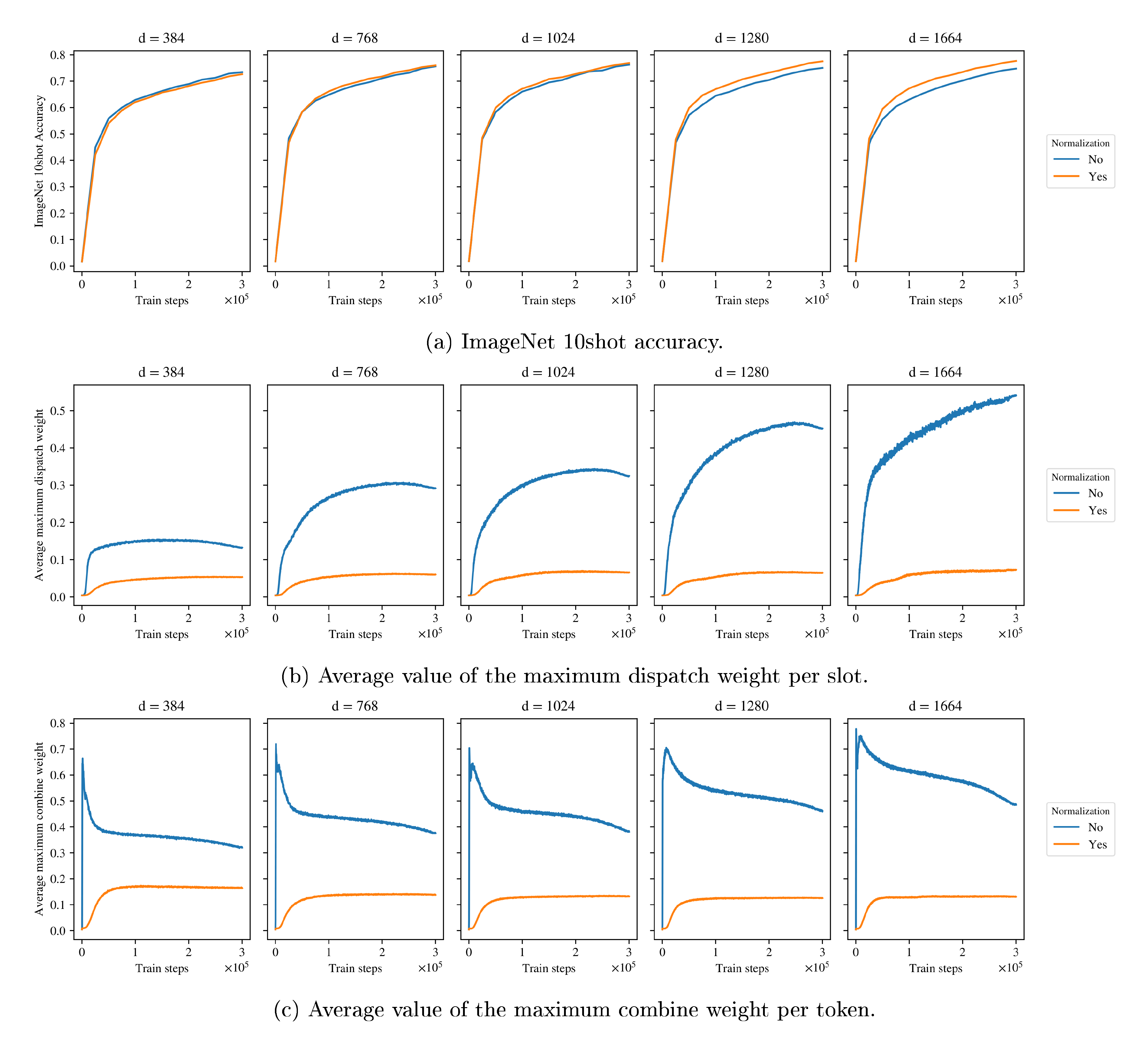
Figure 13 shows different metric curves during the training of a small SoftMoE model with different model dimensions. The model dimensions are those corresponding to different standard backbones: S (384), B (768), L (1024), H (1280) and G (1664). The rest of the architecture parameters are fixed: 6 layers (3 dense layers followed by 3 MoE layers with 256 experts), 14x14 patches, and a MLP dimension of 1536. As the model dimension $d$ increases, the figure shows that, if the inputs to the softmax in the SoftMoE layers are not normalized, the average maximum values of the dispatch and combine weights tend to grow (especially the former). When $d$ is big enough, the ImageNet 10shot accuracy is significantly worse than that achieved by properly normalizing the inputs.
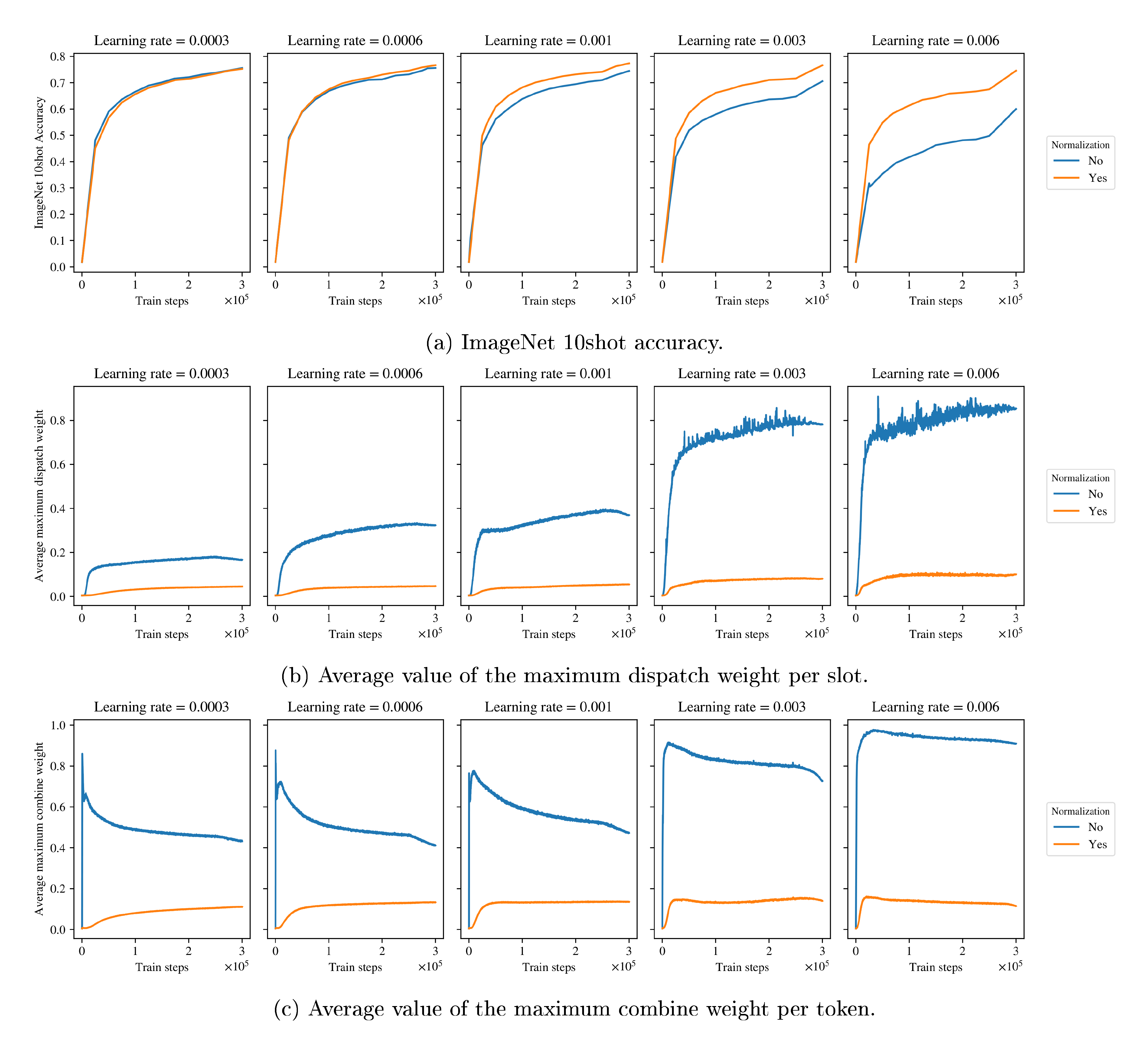
In the previous experiment, we trained our model with a linear decay schedule and a peak value of $10^{-3}$. In addition, we also found that applying the softmax layer directly on the output of layer normalization is also very sensible to the learning rate's configuration. Once again, our recipe suggested in Section 2.3 gives equal or better quality, and is generally more stable. Figure 14 shows different metric curves during the training of the same small SoftMoE model as before, with a model dimension of $d = 1664$, using an inverse square root learning rate schedule, with a fixed timescale of $10^5$, a linear warmup phase of $10^5$ steps, and a linear cooldown of $5 \cdot 10^5$ steps, varying the peak learning rate value. In this figure, similarly to the results from the previous experiment, the average maximum values of the dispatch and combine weights grows to values approaching 1.0 (indicating a collapse in the softmax layers to a one-hot vector), when the inputs to the softmax in the SoftMoE layers are not normalized, which eventually severely hurts the accuracy of the model. However, using the normalization in Section 2.3 gives better accuracy and makes the model less sensible to the choice of the peak value of the learning rate.
F. Additional Results
F.1 Contrastive Learning on LAION-400M
We additionally train a contrastive model, similarly as described on Section 4, but training both the vision and the language towers from scratch on the publicly available dataset LAION-400M[^2] ([21]). The backbone architecture of the vision tower is a B/16. We train one model using a plain Vision Transformer, another one with MoE layers on the second half of the network with 128 experts on each layer, using an Experts Choice router, and a third model using Soft MoE. All the models use the same text tower architecture without MoEs. All the code necessary to replicate the experiments, including the training hyperparameters used, is available at https://github.com/google-research/vmoe.
[^2]: We use in fact a subset of 275M images and text pairs, since many of the original 400M examples could not be downloaded or contained corrupted images (i.e. the decoding of such images failed).
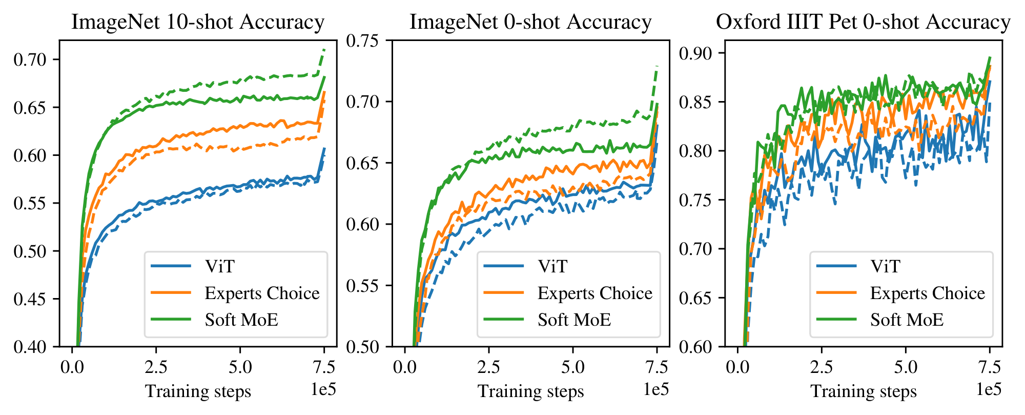
Figure 15 shows that, as with JFT-4B and WebLI pre-training (see Section 3 and Section 4 respectively), when pretraining on the publicly available dataset LAION-400M, Soft MoE performs significantly better than both vanilla Vision Transformers and ViT with Sparse MoE layers using the Experts Choice router, across different downstream metrics. In addition, we can also see that Soft MoE benefits from data augmentation, while neither vanilla ViT or Expert Choice do. Following the observation from Figure 6 in Section 3, we hypothesize that this is because Soft MoE can better utilize the expert parameters.
F.2 The effect of Batch Priority Routing on Tokens Choice routing
Table 8 shows the JFT Precision-at-1 and ImageNet 10-shot Accuracy of S/16 MoE models with Tokens Choice router, with/without using Batch Priority Routing (BPR), for different number of total experts and selected experts per token. This table shows that BPR is especially useful for $K = 1$.
\begin{tabular}{ cccccc }
\toprule
Model & Number of Experts & K & BPR & JFT prec@1 & IN/10shot \\
\midrule
V-MoE S/16 & 32 & 1 & No & 50.1\% & 64.5\% \\
V-MoE S/16 & 32 & 1 & Yes & 51.2\% & 68.9\% \\
\midrule
V-MoE S/16 & 32 & 2 & No & 52.5\% & 71.0\% \\
V-MoE S/16 & 32 & 2 & Yes & 52.8\% & 71.4\% \\
\midrule
V-MoE S/16 & 64 & 1 & No & 50.0\% & 64.4\% \\
V-MoE S/16 & 64 & 1 & Yes & 51.5\% & 69.1\% \\
\midrule
V-MoE S/16 & 64 & 2 & No & 52.9\% & 70.9\% \\
V-MoE S/16 & 64 & 2 & Yes & 52.9\% & 71.4\% \\
\bottomrule
\end{tabular}
F.3 Additional tables and plots complementing Section 3
\begin{tabular}{lrrrrrrrrr}
\toprule
Model & Params & Train steps & Train days & \& exaFLOP & Eval Ms/img & \& GFLOP/img & JFT P@1 & IN/10s & IN/ft\\
\midrule
ViT S/16 & 33M & 4M (50k) & 153.5 & 227.1 & 0.5 & 9.2 & 51.3 & 67.6 & 84.0 \\
\mbox{Soft MoE} S/16 128E & 933M & 4M (50k) & 175.1 & 211.9 & 0.7 & 8.6 & 58.1 & 78.8 & 86.8 \\
\mbox{Soft MoE} S/16 128E & 933M & 10M (50k) & 437.7 & 529.8 & 0.7 & 8.6 & 59.2 & 79.8 & 87.1 \\
\mbox{Soft MoE} S/14 256E & 1.8B & 4M (50k) & 197.9 & 325.7 & 0.9 & 13.2 & 58.9 & 80.0 & 87.2 \\
\mbox{Soft MoE} S/14 256E & 1.8B & 10M (500k) & 494.7 & 814.2 & 0.9 & 13.2 & 60.9 & 80.7 & 87.7 \\
\midrule
ViT B/16 & 108M & 4M (50k) & 410.1 & 864.1 & 1.3 & 35.1 & 56.2 & 76.8 &86.6 \\
\mbox{Soft MoE} B/16 128E & 3.7B & 4M (50k) & 449.5 & 786.4 & 1.5 & 32.0 & 60.0 & 82.0 & 88.0 \\
\midrule
ViT L/16 & 333M & 4M (50k) & 1290.1 & 3025.4 & 4.9 & 122.9 & 59.8 & 81.5 & 88.5 \\
\mbox{Soft MoE} L/16 128E & 13.1B & 1M (50k) & 338.9 & 683.5 & 4.8 & 111.1 & 60.2 & 82.9 & 88.4 \\
\mbox{Soft MoE} L/16 128E & 13.1B & 2M (50k) & 677.7 & 1367.0 & 4.8 & 111.1 & 61.3 & 83.3 & 88.9 \\
\mbox{Soft MoE} L/16 128E & 13.1B & 4M (50k) & 1355.4 & 2734.1 & 4.8 & 111.1 & 61.3 & 83.7 & 88.9 \\
\midrule
ViT H/14 & 669M & 1M (50k) & 1019.9 & 2060.2 & 8.6 & 334.2 & 58.8 & 82.7 & 88.6 \\
ViT H/14 & 669M & 2M (50k) & 2039.8 & 4120.3 & 8.6 & 334.2 & 59.7 & 83.3 & 88.9 \\
\mbox{Soft MoE} H/14 128E & 27.3B & 1M (50k) & 1112.7 & 1754.6 & 8.8 & 284.6 & 61.0 & 83.7 & 88.9 \\
\mbox{Soft MoE} H/14 128E & 27.3B & 2M (50k) & 2225.4 & 3509.2 & 8.8 & 284.6 & 61.7 & 84.2 & 89.1 \\
\mbox{Soft MoE} H/14 256E & 54.1B & 1M (50k) & 1276.9 & 2110.1 & 10.9 & 342.4 & 60.8 & 83.6 & 88.9 \\
\mbox{Soft MoE} H/14 256E & 54.1B & 2M (50k) & 2553.7 & 4220.3 & 10.9 & 342.4 & 62.1 & 84.3 & 89.1 \\
\bottomrule
\end{tabular}
G. Model Inspection
In this section, we take a look at various aspects of the routing the model learns.
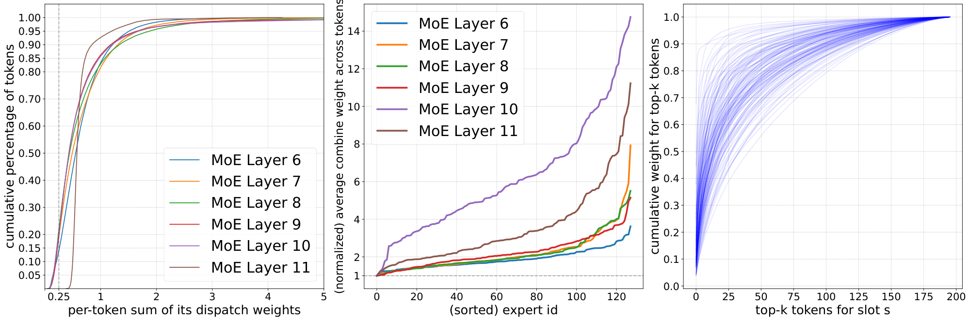
Tokens contributions to slots. While there is no dropping in Soft MoE, it is still possible that some tokens contribute little to all slots if their logits are much lower than those of other tokens. We would like to see if some tokens contribute to slots in a disproportionate manner. Figure 24 (left) shows the distribution across tokens for the total weight each token provides to slots (i.e. summed over all slots). This was computed over a batch with 256 images with 196 tokens each on a Soft MoE S/16 finetuned on ImageNet. We see there is a heavy tail of tokens that provide a stronger total contribution to slots, and the shape is somewhat similar across layers. Around 2-5% of the tokens provide a summed weight above 2. Also, between 15% and 20% of the tokens only contribute up to 0.25 in total weight. The last layer is slightly different, where token contribution is softer tailed. Appendix H further explores this.
Experts contributions to outputs. Similarly, we would like to understand how much different slots end up contributing to the output tokens. We focus on the case of one slot per expert. We can approximate the total contribution of each expert (equivalently, slot) by averaging their corresponding coefficients in the linear combinations for all output tokens in a batch. Figure 24 (center) shows such (normalized) importance across experts for different MoE layers. We see that, depending on the layer, some experts can impact output tokens between 3x and 14x more than others.
Number of input tokens per slot. For each slot, Figure 24 (right) shows how many input tokens are required to achieve a certain cumulative weight in its linear combination. The distribution varies significantly across slots. For a few slots the top 20-25 tokens account for 90% of the slot weight, while for other slots the distribution is more uniform and many tokens contribute to fill in the slot. In general, we see that slots tend to mix a large number of tokens unlike in standard Sparse MoEs.
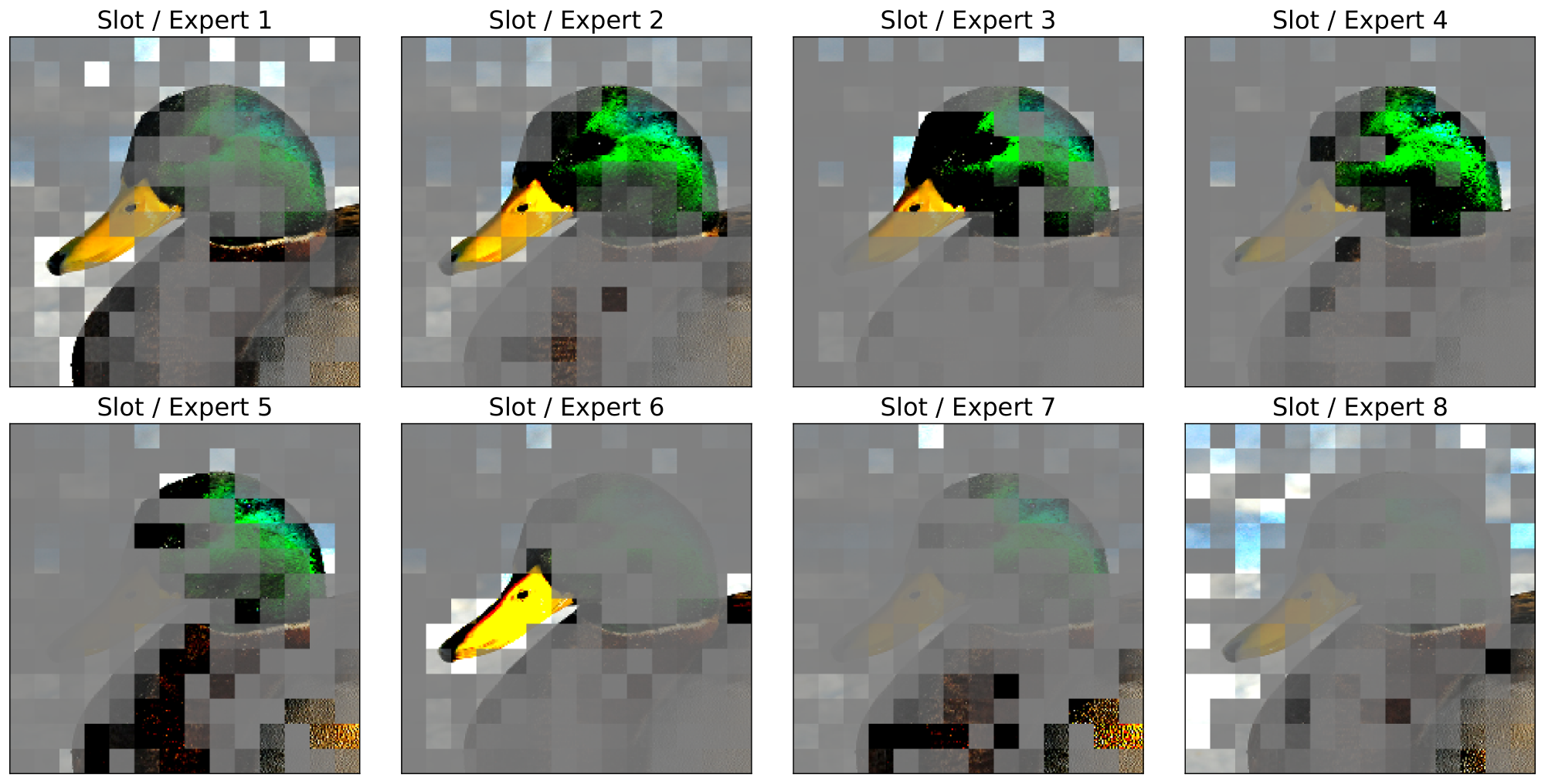
Visual inspection. In order to provide some intuition regarding how slots average input tokens, Figure 25 graphically shows the linear combinations for 8 different slots for the image shown in Figure 1. We shade patches inversely proportionally to their weight in the slots; note that all tokens representations are eventually combined into a single one (with hidden dimension $h$) before being passed to the expert (unlike in our plot, where they are arranged in the usual way). These plots correspond to a Soft MoE S/16 with 128 experts and one slot per expert, and we handpicked 8 out of the 128 slots to highlight how different slots tend to focus on different elements of the image.
H. Additional analysis
H.1 Cumulative sum of dispatch and combine weights
Figure 26 shows the distribution over slots of the cumulative sum (over tokens) of their corresponding dispatch weights. For each slot we compute the cumulative sum of the dispatch weights over tokens sorted in decreasing order. This indicates how many tokens are necessary to cover a given percentage of the total mass of the weighted average. We compute this cumulative sum for all slots over all the 50, 000 ImageNet validation images, across all layers of the Soft MoE H/16 model after finetuning. In the plot, we represent with a solid line the average (over all slots and images) cumulative sum, and the different colored areas represent the central 60%, 80%, 90%, 95% and 99% of the distribution (from darker to lighter colors) of cumulative sums.
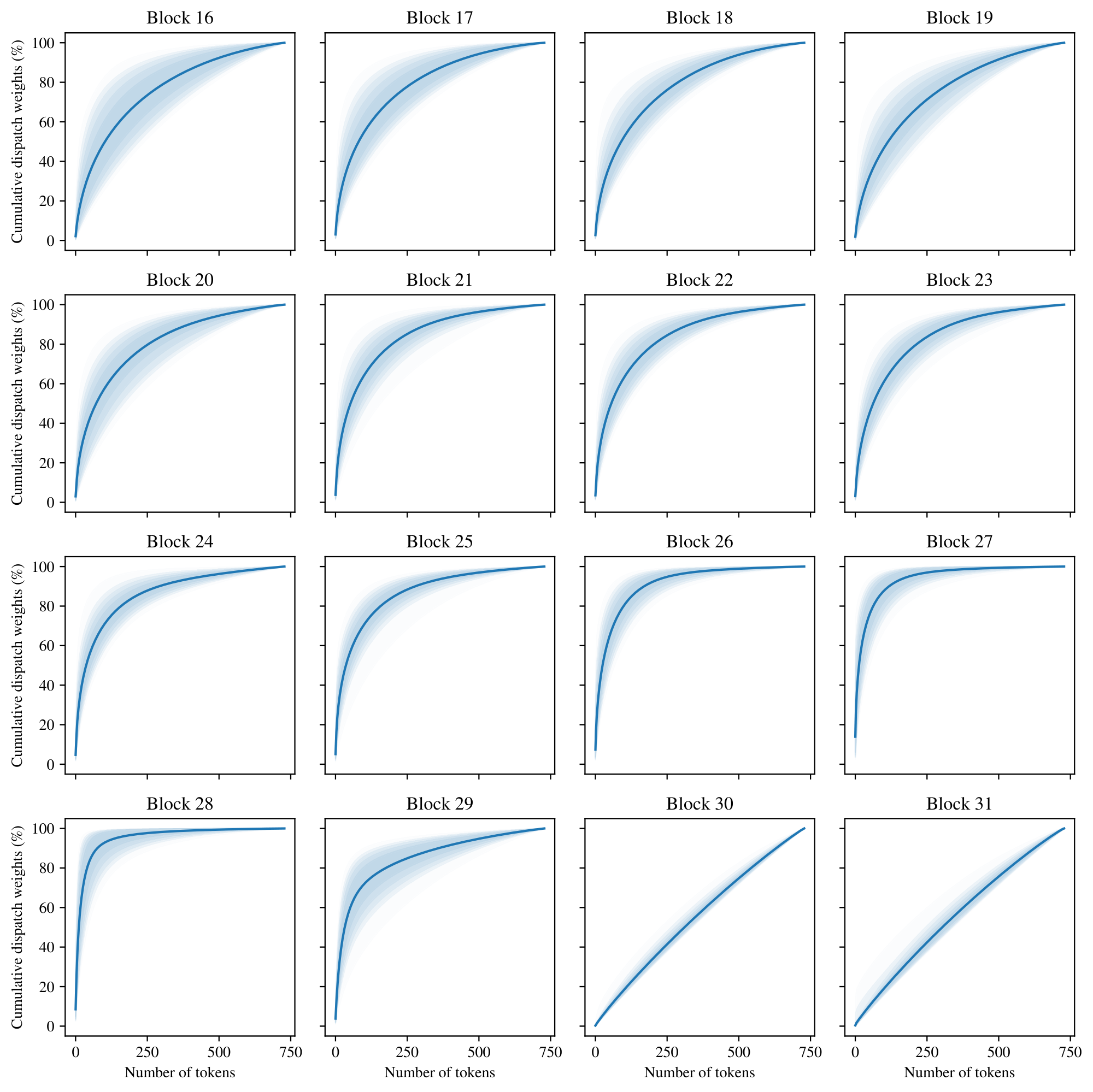
This tells us, for instance, how uniform is the weighted average over tokens used to compute each input slot. In particular, each slot in the last two layers is close to a uniform average of all the tokens (a completely uniform average would be represented by a straight line). This tells us that in these layers, every expert processes roughly the same inputs, at least after the model is trained. However, this weighted average is far from uniform in the rest of the layers, meaning that there are tokens that contribute far more than others. For example, in layer 28, a few tens of tokens already cover 80% of the weighted average mass. Finally, given the width of the colored areas, we can also see that there's a significant difference on the weighted averages depending on the slot, across all layers (except maybe the last two). This indicates that the dispatch weights vary across different slots and images.
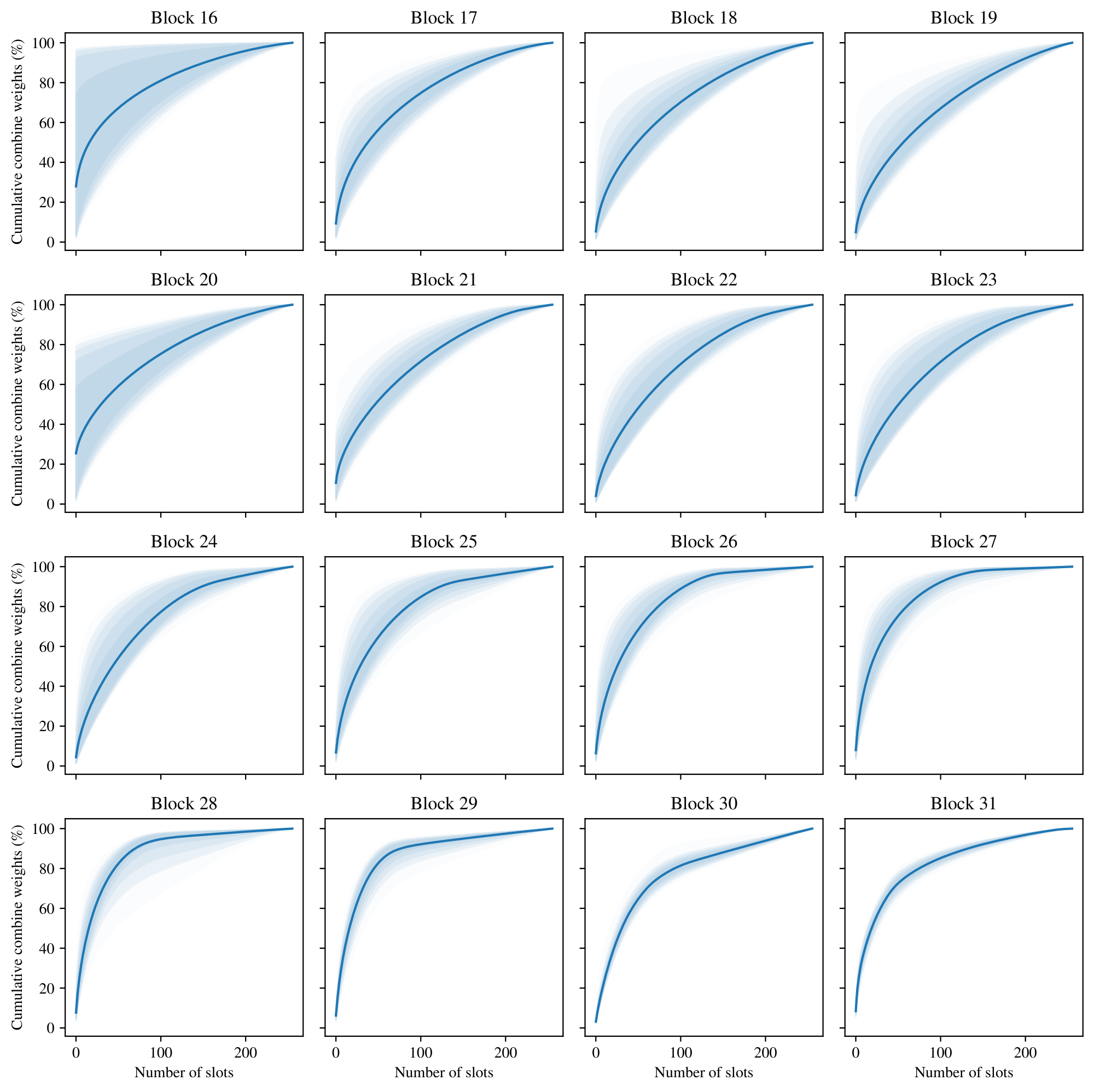
Similarly, Figure 27 shows the corresponding plots for the cumulative sum of the combine weights. In this case, for each output token we compute the cumulative sum of the combine weights over slots sorted in decreasing order. Notice that, although the dispatch weights in the last two layers were almost uniform, the combine weights are not. This indicates that some slots (and thus, experts) are more important than others in computing the output tokens, and thus their corresponding expert parameters are not redundant. Of course, the identity of the "important" slots may vary depending on the input token.
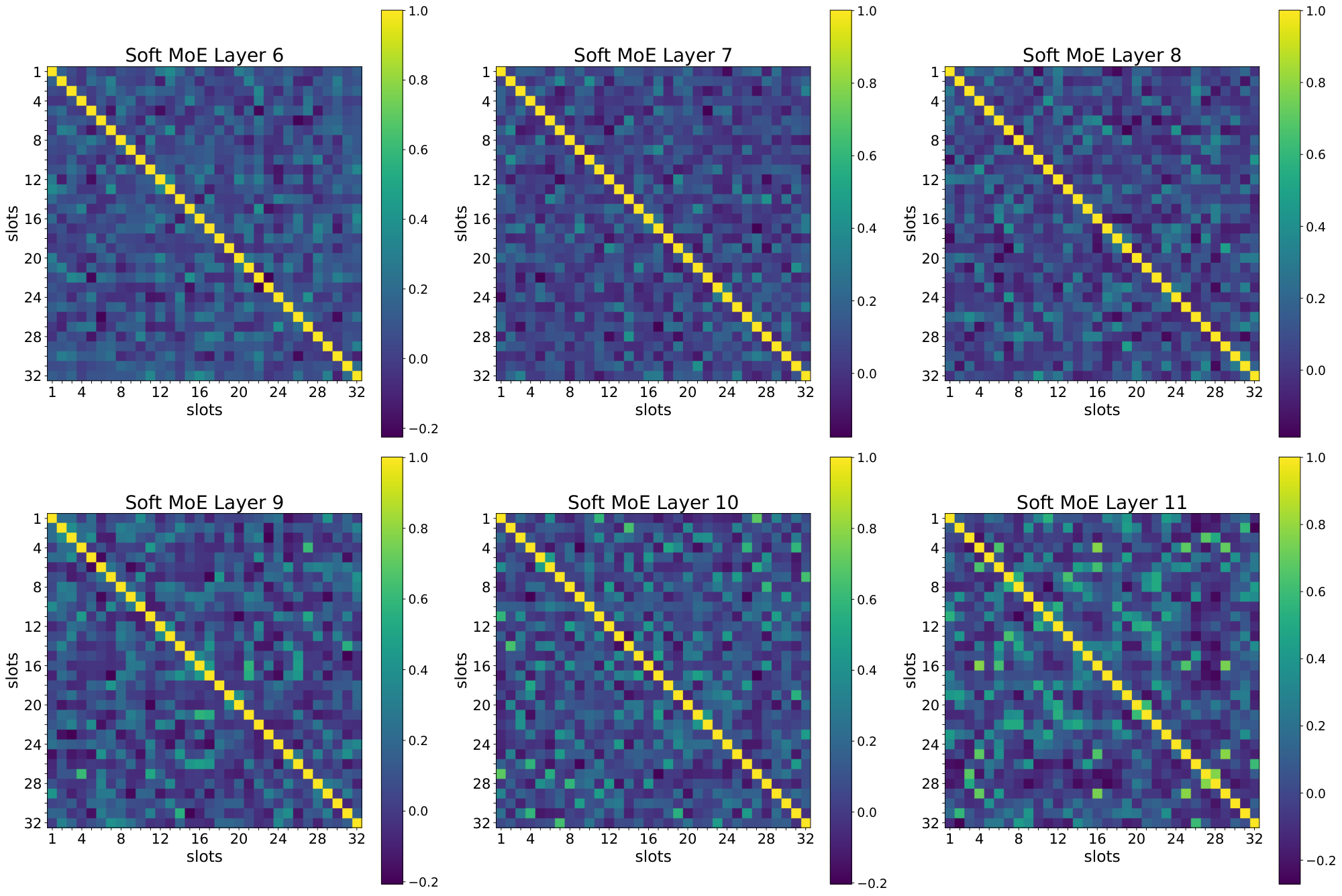
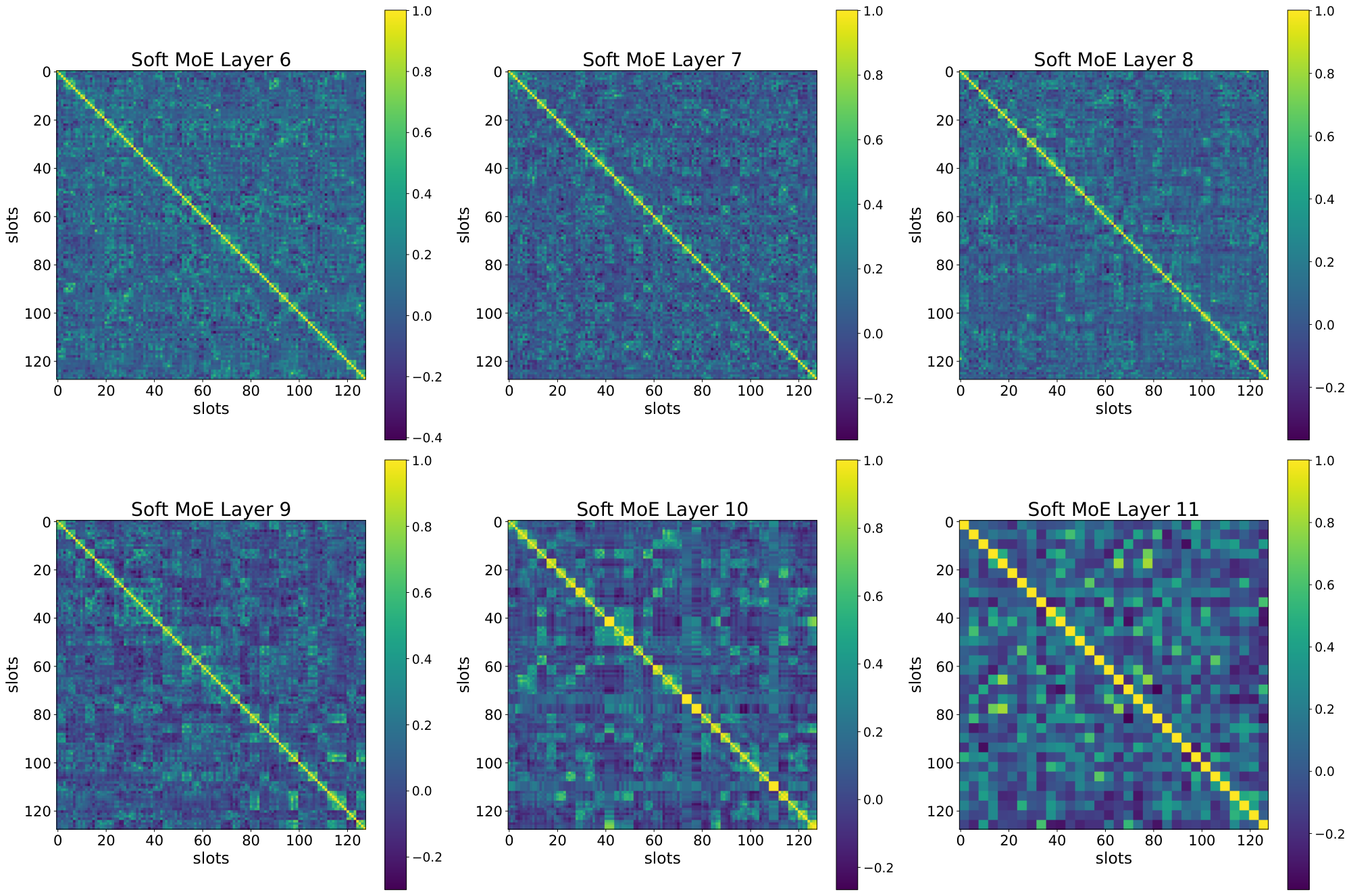
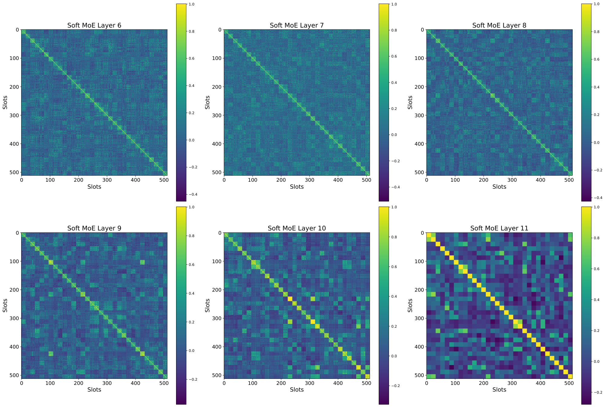
I. Slot Correlation
In this section we explore the correlation between the different slot parameters that Soft MoE learns, and its relationship with the number of slots per expert. Figure 28, Figure 29, and Figure 30 show for each of 6 layers in a Soft MoE S/16 the inner product between each pair of (normalized) slot parameter vectors.
While Figure 28 shows no clear relationship between slots from different experts (as each expert only has one slot), we observe in Figure 29 and Figure 30 how consecutive slots (corresponding to the same expert) are extremely aligned. This confirms our hypothesis that adding more slots to experts does not work very well as these slots end up aligning their value, and computing somewhat similar linear combinations. Therefore, these projections do not add too much useful information to the different tokens to be processed by the experts (in the extreme, these slots would be identical).
J. Pareto Models
Model runs from Section 3.3 (shown in Pareto plot) trained for 300k steps on JFT with inverse square root decay and 50k steps cooldown.
We trained dense and MoE (\mbox{Soft MoE}, Tokens Choice, Experts Choice) models with sizes S/32, S/16, S/8, B/32, B/16, L/32, L/16 and H/14. Sorted by increasing training TPUv3 days."}

\begin{longtable}{lllrrrrrrrr}

\midrule
\endfirsthead

1 & S/32 & Dense & -- & -- & -- & -- & 42.8 & 51.0 & 4.2 & 6.3 \\
2 & S/32 & Experts Choice & 32 & 392 & -- & 0.5 & 45.5 & 56.4 & 3.7 & 6.9 \\
3 & S/32 & Soft MoE & 32 & 49 & -- & -- & 48.2 & 62.3 & 3.8 & 7.0 \\
4 & S/32 & Experts Choice & 32 & 49 & -- & 0.5 & 44.3 & 54.8 & 3.8 & 7.0 \\
5 & S/32 & Experts Choice & 32 & 392 & -- & 1.0 & 46.6 & 58.2 & 4.4 & 7.6 \\
6 & S/32 & Experts Choice & 64 & 392 & -- & 1.0 & 46.7 & 58.4 & 4.4 & 7.8 \\
7 & S/32 & Soft MoE & 64 & 49 & -- & -- & 49.4 & 65.1 & 4.6 & 7.8 \\
8 & S/32 & Experts Choice & 64 & 49 & -- & 1.0 & 45.4 & 56.3 & 4.6 & 7.9 \\
9 & S/32 & Experts Choice & 32 & 49 & -- & 1.0 & 45.5 & 56.9 & 4.6 & 7.9 \\
10 & S/32 & Tokens Choice & 32 & 392 & 1 & 1.0 & 46.3 & 58.7 & 4.4 & 8.0 \\
11 & S/32 & Tokens Choice & 64 & 392 & 1 & 1.0 & 47.1 & 59.4 & 4.4 & 8.1 \\
12 & S/32 & Tokens Choice & 32 & 392 & 2 & 1.0 & 47.4 & 60.3 & 6.0 & 9.3 \\
13 & S/32 & Tokens Choice & 64 & 392 & 2 & 1.0 & 48.0 & 61.9 & 6.0 & 9.8 \\
14 & B/32 & Dense & -- & -- & -- & -- & 48.0 & 63.4 & 16.0 & 11.7 \\
15 & B/32 & Soft MoE & 32 & 49 & -- & -- & 50.9 & 69.7 & 14.3 & 11.7 \\
16 & S/32 & Tokens Choice & 64 & 392 & 2 & 2.0 & 48.9 & 63.9 & 9.0 & 12.0 \\
17 & S/32 & Tokens Choice & 32 & 392 & 2 & 2.0 & 48.5 & 62.8 & 9.1 & 12.1 \\
18 & S/16 & Soft MoE & 16 & 196 & -- & -- & 50.9 & 68.1 & 12.4 & 14.2 \\
19 & S/16 & Soft MoE & 32 & 196 & -- & -- & 52.0 & 70.8 & 12.9 & 14.8 \\
20 & S/16 & Dense & -- & -- & -- & -- & 47.9 & 60.8 & 17.0 & 15.3 \\
21 & S/16 & Soft MoE & 64 & 196 & -- & -- & 52.9 & 72.3 & 13.9 & 15.7 \\
22 & S/16 & Soft MoE & 128 & 196 & -- & -- & 53.6 & 73.0 & 15.9 & 17.6 \\
23 & B/32 & Experts Choice & 32 & 392 & -- & 0.5 & 49.0 & 64.3 & 13.7 & 18.0 \\
24 & B/32 & Experts Choice & 32 & 49 & -- & 0.5 & 47.8 & 62.4 & 14.3 & 18.2 \\
25 & S/16 & Experts Choice & 128 & 196 & -- & 0.5 & 50.2 & 66.7 & 15.8 & 18.5 \\
26 & S/16 & Experts Choice & 32 & 196 & -- & 1.0 & 50.5 & 67.4 & 17.5 & 18.8 \\
27 & S/16 & Experts Choice & 128 & 1568 & -- & 0.5 & 51.4 & 67.7 & 16.8 & 19.7 \\
28 & B/32 & Experts Choice & 32 & 392 & -- & 1.0 & 49.9 & 66.0 & 16.5 & 19.7 \\
29 & B/32 & Experts Choice & 64 & 392 & -- & 1.0 & 49.9 & 65.5 & 16.5 & 19.8 \\
30 & B/32 & Tokens Choice & 32 & 392 & 1 & 1.0 & 49.7 & 66.2 & 16.5 & 20.0 \\
31 & B/32 & Tokens Choice & 64 & 392 & 1 & 1.0 & 49.8 & 65.6 & 16.5 & 20.2 \\
32 & B/32 & Soft MoE & 64 & 49 & -- & -- & 51.8 & 70.7 & 17.8 & 20.3 \\
33 & B/32 & Experts Choice & 64 & 49 & -- & 1.0 & 48.6 & 64.0 & 17.7 & 20.3 \\
34 & B/32 & Experts Choice & 32 & 49 & -- & 1.0 & 48.4 & 63.8 & 17.7 & 20.5 \\
35 & S/16 & Experts Choice & 32 & 1568 & -- & 1.0 & 51.3 & 68.7 & 21.5 & 21.5 \\
36 & S/16 & Soft MoE & 256 & 196 & -- & -- & 53.8 & 73.7 & 19.9 & 22.1 \\
37 & S/16 & Tokens Choice & 32 & 1568 & 1 & 1.0 & 51.2 & 68.9 & 21.5 & 23.2 \\
38 & S/16 & Experts Choice & 256 & 196 & -- & 1.0 & 50.7 & 67.7 & 19.8 & 23.3 \\
39 & S/16 & Experts Choice & 32 & 196 & -- & 2.0 & 51.0 & 68.3 & 23.1 & 23.5 \\
40 & B/32 & Tokens Choice & 32 & 392 & 2 & 1.0 & 50.2 & 67.4 & 22.0 & 23.6 \\
41 & B/32 & Tokens Choice & 64 & 392 & 2 & 1.0 & 50.8 & 68.0 & 22.1 & 23.8 \\
42 & S/16 & Tokens Choice & 64 & 1568 & 1 & 1.0 & 51.5 & 69.1 & 21.3 & 24.9 \\
43 & S/16 & Experts Choice & 256 & 1568 & -- & 1.0 & 52.3 & 69.7 & 21.7 & 25.5 \\
44 & S/16 & Experts Choice & 32 & 1568 & -- & 2.0 & 52.4 & 70.3 & 31.0 & 27.8 \\
45 & S/16 & Tokens Choice & 32 & 1568 & 2 & 1.0 & 52.1 & 70.3 & 31.0 & 30.0 \\
46 & B/32 & Tokens Choice & 64 & 392 & 2 & 2.0 & 51.2 & 70.0 & 33.2 & 30.4 \\
47 & B/32 & Tokens Choice & 32 & 392 & 2 & 2.0 & 51.0 & 69.5 & 33.6 & 31.1 \\
48 & S/16 & Tokens Choice & 64 & 1568 & 2 & 1.0 & 52.3 & 70.4 & 31.1 & 32.0 \\
49 & S/16 & Tokens Choice & 32 & 1568 & 2 & 2.0 & 52.8 & 71.4 & 50.0 & 42.5 \\
50 & S/16 & Tokens Choice & 64 & 1568 & 2 & 2.0 & 52.9 & 71.4 & 50.1 & 45.1 \\
51 & B/16 & Dense & -- & -- & -- & -- & 52.0 & 71.8 & 64.8 & 45.2 \\
52 & B/16 & Soft MoE & 128 & 196 & -- & -- & 55.3 & 77.0 & 59.0 & 46.8 \\
53 & B/16 & Experts Choice & 128 & 1568 & -- & 0.5 & 53.7 & 73.0 & 59.0 & 48.2 \\
54 & B/16 & Experts Choice & 32 & 196 & -- & 1.0 & 53.3 & 73.0 & 65.6 & 51.0 \\
55 & B/16 & Experts Choice & 128 & 196 & -- & 0.5 & 52.5 & 72.2 & 58.8 & 52.6 \\
56 & L/32 & Dense & -- & -- & -- & -- & 51.3 & 70.9 & 55.9 & 54.9 \\
57 & L/32 & Experts Choice & 32 & 392 & -- & 0.5 & 52.3 & 71.2 & 47.4 & 55.2 \\
58 & L/32 & Experts Choice & 32 & 49 & -- & 0.5 & 51.1 & 70.6 & 49.8 & 55.7 \\
59 & L/32 & Soft MoE & 32 & 49 & -- & -- & 53.5 & 75.0 & 49.8 & 56.0 \\
60 & B/16 & Experts Choice & 32 & 1568 & -- & 1.0 & 54.2 & 74.5 & 73.6 & 56.2 \\
61 & B/16 & Tokens Choice & 32 & 1568 & 1 & 1.0 & 53.7 & 74.4 & 73.6 & 57.8 \\
62 & B/16 & Experts Choice & 256 & 196 & -- & 1.0 & 52.7 & 72.7 & 73.4 & 58.1 \\
63 & B/16 & Soft MoE & 256 & 196 & -- & -- & 55.8 & 78.0 & 73.7 & 58.2 \\
64 & B/16 & Tokens Choice & 64 & 1568 & 1 & 1.0 & 54.0 & 74.8 & 73.2 & 58.7 \\
65 & L/32 & Experts Choice & 64 & 392 & -- & 1.0 & 52.7 & 72.1 & 56.9 & 60.4 \\
66 & B/16 & Experts Choice & 256 & 1568 & -- & 1.0 & 53.9 & 73.5 & 73.8 & 60.5 \\
67 & L/32 & Experts Choice & 32 & 392 & -- & 1.0 & 52.7 & 71.7 & 56.8 & 60.6 \\
68 & L/32 & Tokens Choice & 64 & 392 & 1 & 1.0 & 51.9 & 71.4 & 56.9 & 61.0 \\
69 & L/32 & Tokens Choice & 32 & 392 & 1 & 1.0 & 52.3 & 71.7 & 57.1 & 61.6 \\
70 & L/32 & Experts Choice & 64 & 49 & -- & 1.0 & 51.1 & 70.7 & 61.6 & 62.6 \\
71 & L/32 & Soft MoE & 64 & 49 & -- & -- & 54.0 & 75.2 & 61.7 & 62.8 \\
72 & L/32 & Experts Choice & 32 & 49 & -- & 1.0 & 51.4 & 70.3 & 61.5 & 63.2 \\
73 & B/16 & Experts Choice & 32 & 196 & -- & 2.0 & 53.1 & 73.9 & 86.8 & 64.2 \\
74 & L/32 & Tokens Choice & 32 & 392 & 2 & 1.0 & 51.5 & 70.7 & 76.0 & 72.2 \\
75 & B/16 & Experts Choice & 32 & 1568 & -- & 2.0 & 54.6 & 75.6 & 102.9 & 72.5 \\
76 & L/32 & Tokens Choice & 64 & 392 & 2 & 1.0 & 52.0 & 71.8 & 76.0 & 72.5 \\
77 & B/16 & Tokens Choice & 32 & 1568 & 2 & 1.0 & 53.9 & 74.7 & 102.9 & 74.7 \\
78 & B/16 & Soft MoE & 512 & 196 & -- & -- & 56.1 & 78.5 & 103.1 & 76.5 \\
79 & B/16 & Tokens Choice & 64 & 1568 & 2 & 1.0 & 54.3 & 74.8 & 103.0 & 76.5 \\
80 & S/8 & Dense & -- & -- & -- & -- & 49.9 & 66.7 & 82.7 & 77.7 \\
81 & S/8 & Soft MoE & 512 & 784 & -- & -- & 56.1 & 78.0 & 85.6 & 88.5 \\
82 & S/8 & Experts Choice & 32 & 784 & -- & 1.0 & 52.9 & 72.6 & 91.3 & 93.0 \\
83 & L/32 & Tokens Choice & 64 & 392 & 2 & 2.0 & 52.9 & 72.9 & 114.3 & 93.2 \\
84 & L/32 & Tokens Choice & 32 & 392 & 2 & 2.0 & 52.5 & 72.5 & 115.7 & 95.8 \\
85 & L/16 & Dense & -- & -- & -- & -- & 54.8 & 77.8 & 226.9 & 100.9 \\
86 & L/16 & Experts Choice & 128 & 196 & -- & 0.5 & 54.0 & 76.7 & 204.6 & 104.9 \\
87 & L/16 & Soft MoE & 128 & 196 & -- & -- & 57.2 & 80.3 & 205.0 & 106.0 \\
88 & B/16 & Tokens Choice & 32 & 1568 & 2 & 2.0 & 54.4 & 75.7 & 161.4 & 108.4 \\
89 & B/16 & Tokens Choice & 64 & 1568 & 2 & 2.0 & 54.8 & 76.0 & 161.5 & 110.5 \\
90 & L/16 & Experts Choice & 32 & 196 & -- & 1.0 & 55.1 & 77.5 & 228.6 & 113.6 \\
91 & L/16 & Tokens Choice & 32 & 1568 & 1 & 1.0 & 55.9 & 78.5 & 250.4 & 125.1 \\
92 & L/16 & Tokens Choice & 64 & 1568 & 1 & 1.0 & 56.2 & 78.6 & 248.8 & 125.7 \\
93 & S/8 & Experts Choice & 32 & 6272 & -- & 1.0 & 53.6 & 73.4 & 160.6 & 126.6 \\
94 & S/8 & Experts Choice & 512 & 784 & -- & 1.0 & 53.4 & 72.4 & 104.1 & 129.0 \\
95 & L/16 & Soft MoE & 256 & 196 & -- & -- & 57.4 & 80.2 & 256.0 & 129.6 \\
96 & S/8 & Tokens Choice & 32 & 6272 & 1 & 1.0 & 53.8 & 73.7 & 162.5 & 129.8 \\
97 & L/16 & Experts Choice & 256 & 196 & -- & 1.0 & 54.1 & 76.7 & 255.2 & 130.1 \\
98 & L/16 & Experts Choice & 32 & 196 & -- & 2.0 & 55.2 & 77.8 & 301.0 & 140.3 \\
99 & S/8 & Experts Choice & 512 & 6272 & -- & 1.0 & 54.8 & 74.6 & 149.3 & 161.9 \\
100 & S/8 & Tokens Choice & 32 & 6272 & 2 & 1.0 & 54.2 & 74.6 & 243.4 & 166.6 \\
101 & H/14 & Soft MoE & 128 & 256 & -- & -- & 58.0 & 81.6 & 599.2 & 170.5 \\
102 & H/14 & Dense & -- & -- & -- & -- & 56.5 & 80.1 & 680.5 & 196.2 \\
103 & H/14 & Experts Choice & 64 & 2048 & -- & 1.25 & 57.3 & 80.4 & 855.9 & 210.9 \\
104 & L/16 & Tokens Choice & 32 & 1568 & 2 & 2.0 & 53.5 & 74.6 & 534.5 & 218.5 \\
105 & L/16 & Tokens Choice & 64 & 1568 & 2 & 2.0 & 53.3 & 73.3 & 535.1 & 226.9 \\
106 & H/14 & Tokens Choice & 64 & 2048 & 1 & 1.25 & 56.7 & 79.8 & 857.0 & 230.7 \\
107 & S/8 & Tokens Choice & 32 & 6272 & 2 & 2.0 & 54.1 & 74.8 & 424.4 & 255.4 \\
\end{longtable}
References
[1] Jared Kaplan, Sam McCandlish, Tom Henighan, Tom B Brown, Benjamin Chess, Rewon Child, Scott Gray, Alec Radford, Jeffrey Wu, and Dario Amodei. Scaling laws for neural language models. arXiv preprint arXiv:2001.08361, 2020.
[2] Jordan Hoffmann, Sebastian Borgeaud, Arthur Mensch, Elena Buchatskaya, Trevor Cai, Eliza Rutherford, Diego de Las Casas, Lisa Anne Hendricks, Johannes Welbl, Aidan Clark, et al. Training compute-optimal large language models. arXiv preprint arXiv:2203.15556, 2022.
[3] Xiaohua Zhai, Alexander Kolesnikov, Neil Houlsby, and Lucas Beyer. Scaling vision transformers. In Proceedings of the IEEE/CVF Conference on Computer Vision and Pattern Recognition, pages 12104–12113, 2022a.
[4] Dmitry Lepikhin, HyoukJoong Lee, Yuanzhong Xu, Dehao Chen, Orhan Firat, Yanping Huang, Maxim Krikun, Noam Shazeer, and Zhifeng Chen. Gshard: Scaling giant models with conditional computation and automatic sharding. arXiv preprint arXiv:2006.16668, 2020.
[5] William Fedus, Barret Zoph, and Noam Shazeer. Switch transformers: Scaling to trillion parameter models with simple and efficient sparsity. The Journal of Machine Learning Research, 23(1):5232–5270, 2022.
[6] Carlos Riquelme, Joan Puigcerver, Basil Mustafa, Maxim Neumann, Rodolphe Jenatton, André Susano Pinto, Daniel Keysers, and Neil Houlsby. Scaling vision with sparse mixture of experts. Advances in Neural Information Processing Systems, 34:8583–8595, 2021.
[7] Basil Mustafa, Carlos Riquelme, Joan Puigcerver, Rodolphe Jenatton, and Neil Houlsby. Multimodal contrastive learning with limoe: the language-image mixture of experts. arXiv preprint arXiv:2206.02770, 2022.
[8] Mike Lewis, Shruti Bhosale, Tim Dettmers, Naman Goyal, and Luke Zettlemoyer. Base layers: Simplifying training of large, sparse models. In International Conference on Machine Learning, pages 6265–6274. PMLR, 2021.
[9] Emmanuel Bengio, Pierre-Luc Bacon, Joelle Pineau, and Doina Precup. Conditional computation in neural networks for faster models. arXiv preprint arXiv:1511.06297, 2015.
[10] Stephen Roller, Sainbayar Sukhbaatar, Jason Weston, et al. Hash layers for large sparse models. Advances in Neural Information Processing Systems, 34:17555–17566, 2021.
[11] Tianlin Liu, Joan Puigcerver, and Mathieu Blondel. Sparsity-constrained optimal transport. arXiv preprint arXiv:2209.15466, 2022.
[12] Noam Shazeer, Azalia Mirhoseini, Krzysztof Maziarz, Andy Davis, Quoc Le, Geoffrey Hinton, and Jeff Dean. Outrageously large neural networks: The sparsely-gated mixture-of-experts layer. arXiv preprint arXiv:1701.06538, 2017.
[13] Yanqi Zhou, Tao Lei, Hanxiao Liu, Nan Du, Yanping Huang, Vincent Zhao, Andrew M Dai, Quoc V Le, James Laudon, et al. Mixture-of-experts with expert choice routing. Advances in Neural Information Processing Systems, 35:7103–7114, 2022.
[14] Aidan Clark, Diego De Las Casas, Aurelia Guy, Arthur Mensch, Michela Paganini, Jordan Hoffmann, Bogdan Damoc, Blake Hechtman, Trevor Cai, Sebastian Borgeaud, et al. Unified scaling laws for routed language models. In International Conference on Machine Learning, pages 4057–4086. PMLR, 2022.
[15] James Bradbury, Roy Frostig, Peter Hawkins, Matthew James Johnson, Chris Leary, Dougal Maclaurin, George Necula, Adam Paszke, Jake VanderPlas, Skye Wanderman-Milne, et al. JAX: composable transformations of Python+ NumPy programs, 2018.
[16] Tobias Domhan. How much attention do you need? a granular analysis of neural machine translation architectures. In Proceedings of the 56th Annual Meeting of the Association for Computational Linguistics (Volume 1: Long Papers), pages 1799–1808, 2018.
[17] Ruibin Xiong, Yunchang Yang, Di He, Kai Zheng, Shuxin Zheng, Chen Xing, Huishuai Zhang, Yanyan Lan, Liwei Wang, and Tieyan Liu. On layer normalization in the transformer architecture. In International Conference on Machine Learning, pages 10524–10533. PMLR, 2020.
[18] Jia Deng, Wei Dong, Richard Socher, Li-Jia Li, Kai Li, and Li Fei-Fei. Imagenet: A large-scale hierarchical image database. In 2009 IEEE conference on computer vision and pattern recognition, pages 248–255. Ieee, 2009.
[19] Xiaohua Zhai, Xiao Wang, Basil Mustafa, Andreas Steiner, Daniel Keysers, Alexander Kolesnikov, and Lucas Beyer. Lit: Zero-shot transfer with locked-image text tuning. In Proceedings of the IEEE/CVF Conference on Computer Vision and Pattern Recognition, pages 18123–18133, 2022b.
[20] Xi Chen, Xiao Wang, Soravit Changpinyo, AJ Piergiovanni, Piotr Padlewski, Daniel Salz, Sebastian Goodman, Adam Grycner, Basil Mustafa, Lucas Beyer, et al. Pali: A jointly-scaled multilingual language-image model. arXiv preprint arXiv:2209.06794, 2022.
[21] Christoph Schuhmann, Richard Vencu, Romain Beaumont, Robert Kaczmarczyk, Clayton Mullis, Aarush Katta, Theo Coombes, Jenia Jitsev, and Aran Komatsuzaki. LAION-400m: Open dataset of CLIP-filtered 400 million image-text pairs. arXiv preprint arXiv:2111.02114, 2021.
[22] Andrew Jaegle, Felix Gimeno, Andy Brock, Oriol Vinyals, Andrew Zisserman, and Joao Carreira. Perceiver: General perception with iterative attention. In International conference on machine learning, pages 4651–4664. PMLR, 2021.
[23] Michael S Ryoo, AJ Piergiovanni, Anurag Arnab, Mostafa Dehghani, and Anelia Angelova. Tokenlearner: What can 8 learned tokens do for images and videos? arXiv preprint arXiv:2106.11297, 2021.
[24] Cedric Renggli, André Susano Pinto, Neil Houlsby, Basil Mustafa, Joan Puigcerver, and Carlos Riquelme. Learning to merge tokens in vision transformers. arXiv preprint arXiv:2202.12015, 2022.
[25] Yikai Wang, Xinghao Chen, Lele Cao, Wenbing Huang, Fuchun Sun, and Yunhe Wang. Multimodal token fusion for vision transformers. In Proceedings of the IEEE/CVF Conference on Computer Vision and Pattern Recognition (CVPR), pages 12186–12195, June 2022.
[26] Brandon Yang, Gabriel Bender, Quoc V Le, and Jiquan Ngiam. Condconv: Conditionally parameterized convolutions for efficient inference. Advances in Neural Information Processing Systems, 32, 2019.
[27] Zhi Tian, Chunhua Shen, and Hao Chen. Conditional convolutions for instance segmentation. In Computer Vision–ECCV 2020: 16th European Conference, Glasgow, UK, August 23–28, 2020, Proceedings, Part I 16, pages 282–298. Springer, 2020.
[28] Mohammed Muqeeth, Haokun Liu, and Colin Raffel. Soft merging of experts with adaptive routing, 2023.
[29] Xavier Glorot and Yoshua Bengio. Understanding the difficulty of training deep feedforward neural networks. In Proceedings of the thirteenth international conference on artificial intelligence and statistics, pages 249–256. JMLR Workshop and Conference Proceedings, 2010.
[30] Kaiming He, Xiangyu Zhang, Shaoqing Ren, and Jian Sun. Delving deep into rectifiers: Surpassing human-level performance on imagenet classification. In Proceedings of the IEEE international conference on computer vision, pages 1026–1034, 2015.
[31] Günter Klambauer, Thomas Unterthiner, Andreas Mayr, and Sepp Hochreiter. Self-normalizing neural networks. Advances in neural information processing systems, 30, 2017.