GraphRNN: Generating Realistic Graphs with Deep Auto-regressive Models

Jiaxuan You$^{,1}$, Rex Ying$^{,1}$, Xiang Ren$^{2}$, William L. Hamilton$^{1}$, Jure Leskovec$^{1}$

${}^{1}$Department of Computer Science, Stanford University, Stanford, CA, 94305
${}^{2}$Department of Computer Science, University of Southern California, Los Angeles, CA, 90007
${}^{*}$Equal contribution

Correspondence to: Jiaxuan You [email protected].

Proceedings of the $35^{th}$ International Conference on Machine Learning, Stockholm, Sweden, PMLR 80, 2018. Copyright 2018 by the author(s).

Abstract

Modeling and generating graphs is fundamental for studying networks in biology, engineering, and social sciences. However, modeling complex distributions over graphs and then efficiently sampling from these distributions is challenging due to the non-unique, high-dimensional nature of graphs and the complex, non-local dependencies that exist between edges in a given graph. Here we propose GraphRNN, a deep autoregressive model that addresses the above challenges and approximates any distribution of graphs with minimal assumptions about their structure. GraphRNN learns to generate graphs by training on a representative set of graphs and decomposes the graph generation process into a sequence of node and edge formations, conditioned on the graph structure generated so far. In order to quantitatively evaluate the performance of GraphRNN, we introduce a benchmark suite of datasets, baselines and novel evaluation metrics based on Maximum Mean Discrepancy, which measure distances between sets of graphs. Our experiments show that GraphRNN significantly outperforms all baselines, learning to generate diverse graphs that match the structural characteristics of a target set, while also scaling to graphs $50\times$ larger than previous deep models.

Executive Summary: GraphRNN addresses a critical challenge in modeling networks across fields like biology, engineering, and social sciences, where graphs represent complex connections such as molecular structures, social interactions, or citation networks. Traditional methods rely on fixed assumptions about graph structures, like scale-free distributions, which fail to capture real-world diversity and evolve poorly with data. Recent deep learning advances in generating images or text have not fully extended to graphs due to their high dimensionality, variable sizes, and intricate edge dependencies, limiting applications in discovering new structures or simulating evolving networks.

This paper introduces GraphRNN, a deep autoregressive model designed to learn and generate realistic graphs directly from observed examples, approximating any graph distribution without predefined structural rules. The goal is to create a scalable tool that produces diverse graphs matching the input data's characteristics, enabling better simulations and discoveries.

The authors developed GraphRNN by treating graph generation as a sequential process: a graph-level recurrent neural network (RNN) adds nodes one by one, while an edge-level RNN then forms connections for each new node, conditioned on the emerging structure. To handle graphs' non-unique node orderings and ensure efficiency, they impose a breadth-first search ordering during training, reducing computational needs from exponential to roughly quadratic in node count for many cases. The model trains on benchmark datasets of synthetic and real graphs—ranging from 10 to over 2,000 nodes—using maximum likelihood, and generates new graphs autoregressively. Evaluation uses novel metrics based on maximum mean discrepancy (MMD), comparing distributions of key graph properties like degrees, clustering coefficients, and small substructures (motifs), sourced from diverse datasets including community networks, grids, protein structures, and citation graphs over several months of computation on a single GPU.

Key findings highlight GraphRNN's superiority. First, it achieves 80-90% lower MMD scores than traditional models like Erdős-Rényi or Barabási-Albert, and 90% better than prior deep methods like GraphVAE or DeepGMG, across all tested datasets. For instance, on protein graphs with up to 500 nodes, GraphRNN matched degree distributions with MMD of 0.034 versus 0.145 for baselines. Second, a simplified version performed nearly as well on less dependent structures, showing flexibility. Third, it scales to graphs 50 times larger than previous deep models, generating a 2,000-node grid in seconds. Fourth, visualizations and statistics confirm generated graphs capture nuances like community clusters or geometric regularity, even for unseen sizes. Finally, robustness tests showed it maintains low MMD (under 0.1) when interpolating noisy variants of base models, unlike baselines that degrade sharply.

These results mean GraphRNN can produce higher-fidelity synthetic graphs, reducing risks in applications like drug discovery—where inaccurate molecular networks might mislead simulations—or policy modeling of social ties, improving performance and timelines over rigid alternatives. Unlike expectations from prior work limited to small or single graphs, GraphRNN generalizes broadly without domain tweaks, enhancing compliance with real data patterns and cutting costs in data augmentation for machine learning.

Leaders should adopt GraphRNN for graph generation tasks, integrating it into tools for network simulation or augmentation, with the open-source code enabling quick pilots. Trade-offs include choosing the full model for complex dependencies (slower but more accurate) versus the simplified one for speed. Further work needs larger-scale testing, perhaps via pilots on specific domains like bioinformatics, and extensions for conditional generation (e.g., editing edges). Limitations include focus on undirected graphs without initial features, though extensions are outlined, and assumptions like BFS ordering may underperform on highly irregular graphs. Confidence is high for graphs up to thousands of nodes, backed by rigorous benchmarks, but caution applies to extremely dense or directed cases where more validation data would help.

1. Introduction and Related Work

Section Summary: Generative models for graphs, which create realistic network structures like social connections or molecular designs, have long relied on predefined rules that fail to learn directly from real data, missing key features such as community patterns. While recent deep learning techniques like VAEs and GANs have advanced graph generation, they struggle with large, variable graph sizes, multiple ways to represent the same structure, and intricate edge dependencies, limiting them to small or single graphs. This work introduces GraphRNN, a scalable neural network approach that builds graphs step by step using recurrent networks and a smart ordering scheme, along with new benchmarks and rigorous evaluation methods to compare generated graphs against real ones.

Generative models for real-world graphs have important applications in many domains, including modeling physical and social interactions, discovering new chemical and molecular structures, and constructing knowledge graphs. Development of generative graph models has a rich history, and many methods have been proposed that can generate graphs based on a priori structural assumptions [1]. However, a key open challenge in this area is developing methods that can directly learn generative models from an observed set of graphs. Developing generative models that can learn directly from data is an important step towards improving the fidelity of generated graphs, and paves a way for new kinds of applications, such as discovering new graph structures and completing evolving graphs.

In contrast, traditional generative models for graphs (e.g., Barabási-Albert model, Kronecker graphs, exponential random graphs, and stochastic block models) [2, 3, 4, 5, 6, 7] are hand-engineered to model a particular family of graphs, and thus do not have the capacity to directly learn the generative model from observed data. For example, the Barabási-Albert model is carefully designed to capture the scale-free nature of empirical degree distributions, but fails to capture many other aspects of real-world graphs, such as community structure.

Recent advances in deep generative models, such as variational autoencoders (VAE) [8] and generative adversarial networks (GAN) [9], have made important progress towards generative modeling for complex domains, such as image and text data. Building on these approaches a number of deep learning models for generating graphs have been proposed [10, 11, 12, 13]. For example, [12] propose a VAE-based approach, while [13] propose a framework based upon graph neural networks. However, these recently proposed deep models are either limited to learning from a single graph [10, 11] or generating small graphs with 40 or fewer nodes [13, 12]—limitations that stem from three fundamental challenges in the graph generation problem:

• Large and variable output spaces: To generate a graph with $n$ nodes the generative model has to output $n^2$ values to fully specify its structure. Also, the number of nodes $n$ and edges $m$ varies between different graphs and a generative model needs to accommodate such complexity and variability in the output space.
• Non-unique representations: In the general graph generation problem studied here, we want distributions over possible graph structures without assuming a fixed set of nodes (e.g., to generate candidate molecules of varying sizes). In this general setting, a graph with $n$ nodes can be represented by up to $n!$ equivalent adjacency matrices, each corresponding to a different, arbitrary node ordering/numbering. Such high representation complexity is challenging to model and makes it expensive to compute and then optimize objective functions, like reconstruction error, during training. For example, GraphVAE [12] uses approximate graph matching to address this issue, requiring $O(n^4)$ operations in the worst case [14].
• Complex dependencies: Edge formation in graphs involves complex structural dependencies. For example, in many real-world graphs two nodes are more likely to be connected if they share common neighbors [1]. Therefore, edges cannot be modeled as a sequence of independent events, but rather need to be generated jointly, where each next edge depends on the previously generated edges. [13] address this problem using graph neural networks to perform a form of "message passing"; however, while expressive, this approach takes $O(mn^2\mathrm{diam}(G))$ operations to generate a graph with $m$ edges, $n$ nodes and diameter $\mathrm{diam}(G)$.

Present work. Here we address the above challenges and present Graph Recurrent Neural Networks (GraphRNN), a scalable framework for learning generative models of graphs. GraphRNN models a graph in an autoregressive (or recurrent) manner—as a sequence of additions of new nodes and edges—to capture the complex joint probability of all nodes and edges in the graph. In particular, GraphRNN can be viewed as a hierarchical model, where a graph-level RNN maintains the state of the graph and generates new nodes, while an edge-level RNN generates the edges for each newly generated node. Due to its autoregressive structure, GraphRNN can naturally accommodate variable-sized graphs, and we introduce a breadth-first-search (BFS) node-ordering scheme to drastically improve scalability. This BFS approach alleviates the fact that graphs have non-unique representations—by collapsing distinct representations to unique BFS trees—and the tree-structure induced by BFS allows us to limit the number of edge predictions made for each node during training. Our approach requires $O(n^2)$ operations on worst-case (i.e., complete) graphs, but we prove that our BFS ordering scheme permits sub-quadratic complexity in many cases.

In addition to the novel GraphRNN framework, we also introduce a comprehensive suite of benchmark tasks and baselines for the graph generation problem, with all code made publicly available[^1]. A key challenge for the graph generation problem is quantitative evaluation of the quality of generated graphs. Whereas prior studies have mainly relied on visual inspection or first-order moment statistics for evaluation, we provide a comprehensive evaluation setup by comparing graph statistics such as the degree distribution, clustering coefficient distribution and motif counts for two sets of graphs based on variants of the Maximum Mean Discrepancy (MMD) [15]. This quantitative evaluation approach can compare higher order moments of graph-statistic distributions and provides a more rigorous evaluation than simply comparing mean values.

[^1]: The code is available in https://github.com/snap-stanford/GraphRNN, the appendix is available in https://arxiv.org/abs/1802.08773.

Extensive experiments on synthetic and real-world graphs of varying size demonstrate the significant improvement GraphRNN provides over baseline approaches, including the most recent deep graph generative models as well as traditional models. Compared to traditional baselines (e.g., stochastic block models), GraphRNN is able to generate high-quality graphs on all benchmark datasets, while the traditional models are only able to achieve good performance on specific datasets that exhibit special structures. Compared to other state-of-the-art deep graph generative models, GraphRNN is able to achieve superior quantitative performance—in terms of the MMD distance between the generated and test set graphs—while also scaling to graphs that are $50\times$ larger than what these previous approaches can handle. Overall, GraphRNN reduces MMD by $80%\text{-}90%$ over the baselines on average across all datasets and effectively generalizes, achieving comparatively high log-likelihood scores on held-out data.

2. Proposed Approach

Section Summary: The proposed approach, GraphRNN, tackles graph generation by converting graphs into sequences based on different node orderings, making it possible to use autoregressive models like those for text to learn and create new graphs step by step. It avoids pitfalls of earlier methods, such as struggling with varying graph sizes or needing to process all possible node arrangements, by employing two types of recurrent neural networks: one to add nodes sequentially and another to predict connections for each new node to its predecessors. This framework learns from one or more example graphs and generates realistic new ones while efficiently handling complex edge patterns.

We first describe the background and notation for building generative models of graphs, and then describe our autoregressive framework, GraphRNN.

2.1 Notations and Problem Definition

An undirected graph[^2] $G=(V, E)$ is defined by its node set $V={v_1, ..., v_n}$ and edge set $E={(v_i, v_j)|v_i, v_j\in V}$. One common way to represent a graph is using an adjacency matrix, which requires a node ordering $\pi$ that maps nodes to rows/columns of the adjacency matrix. More precisely, $\pi$ is a permutation function over $V$ (i.e., $(\pi(v_1), ..., \pi(v_n))$ is a permutation of $(v_1, ..., v_n)$). We define $\Pi$ as the set of all $n!$ possible node permutations. Under a node ordering $\pi$, a graph $G$ can then be represented by the adjacency matrix $A^{\pi}\in\mathbb{R}^{n\times n}$, where $A^\pi_{i, j} = \mathds{1}[(\pi(v_i), \pi(v_j))\in E]$. Note that elements in the set of adjacency matrices $A^\Pi={A^\pi|\pi\in\Pi}$ all correspond to the same underlying graph.

[^2]: We focus on undirected graphs. Extensions to directed graphs and graphs with features are discussed in the Appendix.

The goal of learning generative models of graphs is to learn a distribution $p_{model}(G)$ over graphs, based on a set of observed graphs $\mathbb{G}={G_1, ..., G_s}$ sampled from data distribution $p(G)$, where each graph $G_i$ may have a different number of nodes and edges. When representing $G\in\mathbb{G}$, we further assume that we may observe any node ordering $\pi$ with equal probability, i.e., $p(\pi)=\frac{1}{n!}, \forall\pi\in\Pi$. Thus, the generative model needs to be capable of generating graphs where each graph could have exponentially many representations, which is distinct from previous generative models for images, text, and time series.

Finally, note that traditional graph generative models (surveyed in the introduction) usually assume a single input training graph. Our approach is more general and can be applied to a single as well as multiple input training graphs.

2.2 A Brief Survey of Possible Approaches

We start by surveying some general alternative approaches for modeling $p(G)$, in order to highlight the limitations of existing non-autoregressive approaches and motivate our proposed autoregressive architecture.

Vector-representation based models. One naïve approach would be to represent $G$ by flattening $A^\pi$ into a vector in $\mathbb{R}^{n^2}$, which is then used as input to any off-the-shelf generative model, such as a VAE or GAN. However, this approach suffers from serious drawbacks: it cannot naturally generalize to graphs of varying size, and requires training on all possible node permutations or specifying a canonical permutation, both of which require $O(n!)$ time in general.

Node-embedding based models. There have been recent successes in encoding a graph's structural properties into node embeddings [16], and one approach to graph generation could be to define a generative model that decodes edge probabilities based on pairwise relationships between learned node embeddings (as in [10]). However, this approach is only well-defined when given a fixed-set of nodes, limiting its utility for the general graph generation problem, and approaches based on this idea are limited to learning from a single input graph [10, 11].

2.3 GraphRNN: Deep Generative Models for Graphs

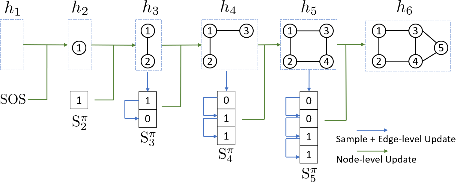
The key idea of our approach is to represent graphs under different node orderings as sequences, and then to build an autoregressive generative model on these sequences. \ As we will show, this approach does not suffer from the drawbacks common to other general approaches (c.f., Section 2.2), allowing us to model graphs of varying size with complex edge dependencies, and we introduce a BFS node ordering scheme to drastically reduce the complexity of learning over all possible node sequences (Section 2.3.4). In this autoregressive framework, the model complexity is greatly reduced by weight sharing with recurrent neural networks (RNNs). Figure 1 illustrates our GraphRNN approach, where the main idea is that we decompose graph generation into a process that generates a sequence of nodes (via a graph-level RNN), and another process that then generates a sequence of edges for each newly added node (via an edge-level RNN).

2.3.1 Modeling graphs as sequences

We first define a mapping $f_S$ from graphs to sequences, where for a graph $G\sim p(G)$ with $n$ nodes under node ordering $\pi$, we have

$ S^\pi=f_S(G, \pi)=(S^\pi_1, ..., S^\pi_{n}),\tag{1} $

where each element $S^\pi_i\in {0, 1}^{i-1}, i\in {1, ..., n}$ is an adjacency vector representing the edges between node $\pi(v_{i})$ and the previous nodes $\pi(v_{j}), j\in {1, ..., i-1}$ already in the graph:[^3]

[^3]: We prohibit self-loops and $S^\pi_1$ is defined as an empty vector.

$ S^\pi_i = (A^\pi_{1, i}, ..., A^\pi_{i-1, i})^T, \forall i\in {2, ..., n}. $

For undirected graphs, $S^\pi$ determines a unique graph $G$, and we write the mapping as $f_G(\cdot)$ where $f_G(S^{\pi})=G$.

Thus, instead of learning $p(G)$, whose sample space cannot be easily characterized, we sample the auxiliary $\pi$ to get the observations of $S^\pi$ and learn $p(S^\pi)$, which can be modeled autoregressively due to the sequential nature of $S^\pi$. At inference time, we can sample $G$ without explicitly computing $p(G)$ by sampling $S^\pi$, which maps to $G$ via $f_G$.

Given the above definitions, we can write $p(G)$ as the marginal distribution of the joint distribution $p(G, S^\pi)$:

$ p(G) = \sum_{S^\pi}{ p(S^\pi) \ \mathds{1}[f_G(S^\pi)=G]},\tag{2} $

where $p(S^\pi)$ is the distribution that we want to learn using a generative model. Due to the sequential nature of $S^\pi$, we further decompose $p(S^\pi)$ as the product of conditional distributions over the elements:

$ p(S^\pi) = \prod_{i=1}^{n+1}{p(S^\pi_i|S^\pi_1, ..., S^\pi_{i-1})} $

where we set $S^\pi_{n+1}$ as the end of sequence token $\texttt{EOS}$, to represent sequences with variable lengths. We simplify $p(S^\pi_i|S^\pi_1, ..., S^\pi_{i-1})$ as $p(S^\pi_i|S^\pi_{<i})$ in further discussions.

\addtocounter{ALC@line}{1}\addtocounter{ALC@rem}{1}\ifthenelse{\equal{\arabic{ALC@rem}}{#1}}{\setcounter{ALC@rem}{0}}{}\item **Input:** RNN-based transition module $f_{trans}$, output module $f_{out}$, probability distribution $\mathcal{P}_{\theta_i}$ parameterized by $\theta_i$, start token $\texttt{SOS}$, end token $\texttt{EOS}$, empty graph state $h'$
\addtocounter{ALC@line}{1}\addtocounter{ALC@rem}{1}\ifthenelse{\equal{\arabic{ALC@rem}}{#1}}{\setcounter{ALC@rem}{0}}{}\item **Output:** Graph sequence $S^{\pi}$
\addtocounter{ALC@line}{1}\addtocounter{ALC@rem}{1}\ifthenelse{\equal{\arabic{ALC@rem}}{#1}}{\setcounter{ALC@rem}{0}}{}\item $S^{\pi}_1=\texttt{SOS}$, $h_1 =  h'$, $i=1$
\addtocounter{ALC@line}{1}\addtocounter{ALC@rem}{1}\ifthenelse{\equal{\arabic{ALC@rem}}{#1}}{\setcounter{ALC@rem}{0}}{}\item **repeat**
\ifthenelse{\equal{##default}{default}}
{}{\ \{##default\}}

algorithm \ifthenelse{\equal{\arabic{ALC@rem}}{#1}}\item $i=i+1$ \ifthenelse{\equal{\arabic{ALC@rem}}{#1}}\item $h_i = f_{\mathrm{trans}}( h_{i-1},S^{\pi}{i-1})$ {#update graph state} \ifthenelse{\equal{\arabic{ALC@rem}}{#1}}\item $\theta_i = f{\mathrm{out}}(h_i)$ \ifthenelse{\equal{\arabic{ALC@rem}}{#1}}\item $S^{\pi}i \sim \mathcal{P}{\theta_i}$ {#sample node $i$ 's edge connections}

\addtocounter{ALC@line}{1}\addtocounter{ALC@rem}{1}\ifthenelse{\equal{\arabic{ALC@rem}}{#1}}{\setcounter{ALC@rem}{0}}{}\item **until**\ # $S^{\pi}_i$ is $\texttt{EOS}$
\addtocounter{ALC@line}{1}\addtocounter{ALC@rem}{1}\ifthenelse{\equal{\arabic{ALC@rem}}{#1}}{\setcounter{ALC@rem}{0}}{}\item **Return** $S^{\pi}=(S^{\pi}_1,...,S^{\pi}_i)$

2.3.2 The GraphRNN framework

So far we have transformed the modeling of $p(G)$ to modeling $p(S^{\pi})$, which we further decomposed into the product of conditional probabilities $p(S^\pi_i|S^\pi_{<i})$. Note that $p(S^\pi_i|S^\pi_{<i})$ is highly complex as it has to capture how node $\pi(v_i)$ links to previous nodes based on how previous nodes are interconnected among each other. Here we propose to parameterize $p(S^\pi_i|S^\pi_{<i})$ using expressive neural networks to model the complex distribution. To achieve scalable modeling, we let the neural networks share weights across all time steps $i$. In particular, we use an RNN that consists of a state-transition function and an output function:

$ \begin{align} h_i &= f_{\mathrm{trans}}({h}{i-1}, S^\pi{i-1}), @centercr \theta_{i} &= f_{\mathrm{out}}({h}_i), \end{align}\tag{3} $

where $ h_i \in \mathbb{R}^{d}$ is a vector that encodes the state of the graph generated so far, $S^\pi_{i-1}$ is the adjacency vector for the most recently generated node $i-1$, and $\theta_i$ specifies the distribution of next node's adjacency vector (i.e., $S^{\pi}i \sim \mathcal{P}{\theta_i}$). In general, $f_{\mathrm{trans}}$ and $f_{\mathrm{out}}$ can be arbitrary neural networks, and $\mathcal{P}_{\theta_i}$ can be an arbitrary distribution over binary vectors. This general framework is summarized in Algorithm 1.

Note that the proposed problem formulation is fully general; we discuss and present some specific variants with implementation details in the next section. Note also that RNNs require fixed-size input vectors, while we previously defined $S^\pi_i$ as having varying dimensions depending on $i$; we describe an efficient and flexible scheme to address this issue in Section 2.3.4.

2.3.3 GraphRNN variants

Different variants of the GraphRNN model correspond to different assumptions about $p(S^\pi_i|S^\pi_{<i})$. Recall that each dimension of $S^\pi_i$ is a binary value that models existence of an edge between the new node $\pi(v_{i})$ and a previous node $\pi(v_{j}), j\in {1, ..., i-1}$. We propose two variants of GraphRNN, both of which implement the transition function $f_{\mathrm{trans}}$ (i.e., the graph-level RNN) as a Gated Recurrent Unit (GRU) [17] but differ in the implementation of $f_{\mathrm{out}}$ (i.e., the edge-level model). Both variants are trained using stochastic gradient descent with a maximum likelihood loss over $S^\pi$ — i.e., we optimize the parameters of the neural networks to optimize $\prod{p_{model}(S^\pi)}$ over all observed graph sequences.

Multivariate Bernoulli. First we present a simple baseline variant of our GraphRNN approach, which we term GraphRNN-S ("S" for "simplified"). In this variant, we model $p(S^\pi_i|S^\pi_{<i})$ as a multivariate Bernoulli distribution, parameterized by the $\theta_i\in \mathbb{R}^{i-1}$ vector that is output by $f_{\mathrm{out}}$. In particular, we implement $f_{\mathrm{out}}$ as single layer multi-layer perceptron (MLP) with sigmoid activation function, that shares weights across all time steps. The output of $f_{\mathrm{out}}$ is a vector $\theta_i$, whose element $\theta_{i}[j]$ can be interpreted as a probability of edge $(i, j)$. We then sample edges in $S^\pi_i$ independently according to a multivariate Bernoulli distribution parametrized by $\theta_i$.

Dependent Bernoulli sequence. To fully capture complex edge dependencies, in the full GraphRNN model we further decompose $p(S^\pi_i|S^\pi_{<i})$ into a product of conditionals,

$ p(S^\pi_i|S^\pi_{<i}) = \prod_{j=1}^{i-1} p(S^\pi_{i, j} | S^\pi_{i, <j}, S^\pi_{<i}),\tag{4} $

where $S^\pi_{i, j}$ denotes a binary scalar that is $1$ if node $\pi(v_{i+1})$ is connected to node $\pi(v_{j})$ (under ordering $\pi$). In this variant, each distribution in the product is approximated by an another RNN. Conceptually, we have a hierarchical RNN, where the first (i.e., the graph-level) RNN generates the nodes and maintains the state of the graph, while the second (i.e., the edge-level) RNN generates the edges of a given node (as illustrated in Figure 1). In our implementation, the edge-level RNN is a GRU model, where the hidden state is initialized via the graph-level hidden state $h_i$ and where the output at each step is mapped by a MLP to a scalar indicating the probability of having an edge. $S^\pi_{i, j}$ is sampled from this distribution specified by the $j$ th output of the $i$ th edge-level RNN, and is fed into the $j+1$ th input of the same RNN. All edge-level RNNs share the same parameters.

2.3.4 Tractability via breadth-first search

A crucial insight in our approach is that rather than learning to generate graphs under any possible node permutation, we learn to generate graphs using breadth-first-search (BFS) node orderings, without a loss of generality. Formally, we modify Equation (1) to

$ S^\pi=f_S(G, \textsc{BFS}(G, \pi)),\tag{5} $

where $\textsc{BFS}(\cdot)$ denotes the deterministic BFS function. In particular, this BFS function takes a random permutation $\pi$ as input, picks $\pi(v_1)$ as the starting node and appends the neighbors of a node into the BFS queue in the order defined by $\pi$. Note that the BFS function is many-to-one, i.e., multiple permutations can map to the same ordering after applying the BFS function.

Using BFS to specify the node ordering during generation has two essential benefits. The first is that we only need to train on all possible BFS orderings, rather than all possible node permutations, i.e., multiple node permutations map to the same BFS ordering, providing a reduction in the overall number of sequences we need to consider.[^4] The second is that the BFS ordering makes learning easier by reducing the number of edge predictions we need to make in the edge-level RNN; in particular, when we are adding a new node under a BFS ordering, the only possible edges for this new node are those connecting to nodes that are in the "frontier" of the BFS (i.e., nodes that are still in the BFS queue)—a notion formalized by Proposition 1 (proof in the Appendix):

[^4]: In the worst case (e.g., star graphs), the number of BFS orderings is $n!$, but we observe substantial reductions on many real-world graphs.

########## {caption="Proposition 1"}

Suppose $v_1, \ldots, v_n$ is a BFS ordering of $n$ nodes in graph $G$, and $(v_i, v_{j-1}) \in E$ but $(v_i, v_j) \not \in E$ for some $i < j \le n$, then $(v_{i'}, v_{j'}) \not \in E$, $\forall 1 \le i' \le i$ and $j \le j' < n$.

Importantly, this insight allows us to redefine the variable size $S^\pi_i$ vector as a fixed $M$-dimensional vector, representing the connectivity between node $\pi(v_i)$ and nodes in the current BFS queue with maximum size $M$:

$ S^\pi_i = (A^\pi_{\max(1, i-M), i}, ..., A^\pi_{i-1, i})^T, i\in {2, ..., n}. $

As a consequence of Proposition 1, we can bound $M$ as follows:

########## {type="Corollary"}

With a BFS ordering the maximum number of entries that GraphRNN model needs to predict for $S^\pi_i$, $\forall 1 \le i \le n$ is $O\left(\max_{d=1}^{\mathrm{diam}(G)} \left|\left{v_i | \mathrm{dist}(v_i, v_1) = d\right} \right| \right)$, where $\mathrm{dist}$ denotes the shortest-path-distance between vertices.

The overall time complexity of GraphRNN is thus $O(Mn)$. In practice, we estimate an empirical upper bound for $M$ (see the Appendix for details).

3. GraphRNN Model Capacity

Section Summary: This section explores the GraphRNN model's ability to represent and generate complex graph structures by examining its handling of edge connections. It first shows how GraphRNN can learn to produce graphs with a global community structure, where nodes are divided into two groups with denser connections inside groups than between them, relying on the model's memory of past node assignments to predict new edges accurately. Additionally, GraphRNN can create regular geometric patterns, such as ladder graphs, by tracking node degrees and making precise connection decisions based on prior connections to maintain the structured layout.

In this section we analyze the representational capacity of GraphRNN, illustrating how it is able to capture complex edge dependencies. In particular, we discuss two very different cases on how GraphRNN can learn to generate graphs with a global community structure as well as graphs with a very regular geometric structure. For simplicity, we assume that $h_i$ (the hidden state of the graph-level RNN) can exactly encode $S^\pi_{<i}$, and that the edge-level RNN can encode $S^\pi_{i, <j}$. That is, we assume that our RNNs can maintain memory of the decisions they make and elucidate the models capacity in this ideal case. We similarly rely on the universal approximation theorem of neural networks [18].

Graphs with community structure. GraphRNN can model structures that are specified by a given probabilistic model. This is because the posterior of a new edge probability can be expressed as a function of the outcomes of previous nodes. For instance, suppose that the training set contains graphs generated from the following distribution $p_{com}(G)$: half of the nodes are in community $A$, and half of the nodes are in community $B$ (in expectation), and nodes are connected with probability $p_s$ within each community and probability $p_d$ between communities. Given such a model, we have the following key (inductive) observation:

########## {caption="\textbf{Observation 2"}

Assume there exists a parameter setting for GraphRNN such that it can generate $S^\pi_{<i}$ and $S^\pi_{i, <j}$ according to the distribution over $S^\pi$ implied by $p_{com}(G)$, then there also exists a parameter setting for GraphRNN such that it can output $p(S^\pi_{i, j} | S^\pi_{i, <j}, S^\pi_{<i})$ according to $p_{com}(G)$.

This observation follows from three facts: First, we know that $p(S^\pi_{i, j} | S^\pi_{i, <j}, S^\pi_{<i})$ can be expressed as a function of $p_s$, $p_d$, and $p(\pi(v_j) \in A), p(\pi(v_j) \in B) : \forall 1 \leq j \le i$ (which holds by $p_{com}$ 's definition). Second, by our earlier assumptions on the RNN memory, $S^\pi_{<i}$ can be encoded into the initial state of the edge-level RNN, and the edge-level RNN can also encode the outcomes of $S^\pi_{i, <j}$. Third, we know that $p(\pi(v_i) \in A)$ is computable from $S^\pi_{<i}$ and $S^\pi_{i, 1}$ (by Bayes' rule and $p_{com}$ 's definition, with an analogous result for $p(\pi(v_i) \in B)$). Finally, GraphRNN can handle the base case of the induction in \textbf{Observation 2, i.e., $S_{i, 1}$, simply by sampling according to $0.5p_s + 0.5p_d$ at the first step of the edge-level RNN (i.e., 0.5 probability $i$ is in same community as node $\pi(v_1)$).

Graphs with regular structure. GraphRNN can also naturally learn to generate regular structures, due to its ability to learn functions that only activate for $S^\pi_{i, j}$ where $v_j$ has specific degree. For example, suppose that the training set consists of ladder graphs [19]. To generate a ladder graph, the edge-level RNN must handle three key cases: if $\sum_{k=1}^{j}S^\pi_{i, j} = 0$, then the new node should only connect to the degree $1$ node or else any degree $2$ node; if $\sum_{k=1}^{j}S^\pi_{i, j} = 1$, then the new node should only connect to the degree $2$ node that is exactly two hops away; and finally, if $\sum_{k=1}^{j}S^\pi_{i, j} = 2$ then the new node should make no further connections. And note that all of the statistics needed above are computable from $S^\pi_{<i}$ and $S^\pi_{i, <j}$. The appendix contains visual illustrations and further discussions on this example.

4. Experiments

Section Summary: The experiments evaluate GraphRNN, a graph generation model, against traditional and deep learning baselines on synthetic and real-world datasets, including community structures, grid patterns, citation networks, and protein structures, with graph sizes ranging from 10 to over 2,000 nodes. Researchers tested on 80% training and 20% held-out data, using metrics like maximum mean discrepancy to assess how well generated graphs match originals in properties such as node degrees, clustering, and structural motifs. Overall, GraphRNN outperforms competitors, producing higher-quality graphs that closely resemble the training data, especially on larger and more complex examples where other methods struggle with scalability.

We compare GraphRNN to state-of-the-art baselines, demonstrating its robustness and ability to generate high-quality graphs in diverse settings.

4.1 Datasets

We perform experiments on both synthetic and real datasets, with drastically varying sizes and characteristics. The sizes of graphs vary from $|V|=10$ to $|V|=2025$.

Community. 500 two-community graphs with $60\leq|V|\leq160$. Each community is generated by the Erdős-Rényi model (E-R) [2] with $n=|V|/2$ nodes and $p=0.3$. We then add $0.05|V|$ inter-community edges with uniform probability.

Grid. 100 standard 2D grid graphs with $100\leq|V|\leq400$. We also run our models on 100 standard 2D grid graphs with $1296\leq|V|\leq2025$, and achieve comparable results.

B-A. 500 graphs with $100\leq|V|\leq200$ that are generated using the Barabási-Albert model. During generation, each node is connected to 4 existing nodes.

Protein. 918 protein graphs [20] with $100\leq|V|\leq500$. Each protein is represented by a graph, where nodes are amino acids and two nodes are connected if they are less than $6$ Angstroms apart.

Ego. 757 3-hop ego networks extracted from the Citeseer network [21] with $50\leq|V|\leq399$. Nodes represent documents and edges represent citation relationships.

4.2 Experimental Setup

We compare the performance of our model against various traditional generative models for graphs, as well as some recent deep graph generative models.

Traditional baselines. Following [13] we compare against the Erdős-Rényi model (E-R) [2] and the Barabási-Albert (B-A) model [4]. In addition, we compare against popular generative models that include learnable parameters: Kronecker graph models [3] and mixed-membership stochastic block models (MMSB) [5].

Deep learning baselines. We compare against the recent methods of [12] (GraphVAE) and [13] (DeepGMG). We provide reference implementations for these methods (which do not currently have associated public code), and we adapt GraphVAE to our problem setting by using one-hot indicator vectors as node features for the graph convolutional network encoder.[^5]

[^5]: We also attempted using degree and clustering coefficients as features for nodes, but did not achieve better performance.

Experiment settings. We use $80%$ of the graphs in each dataset for training and test on the rest. We set the hyperparameters for baseline methods based on recommendations made in their respective papers. The hyperparameter settings for GraphRNN were fixed after development tests on data that was not used in follow-up evaluations (further details in the Appendix). Note that all the traditional methods are only designed to learn from a single graph, therefore we train a separate model for each training graph in order to compare with these methods. In addition, both deep learning baselines suffer from aforementioned scalability issues, so we only compare to these baselines on a small version of the community dataset with $12\leq|V|\leq20$ (Community-small) and 200 ego graphs with $4\leq|V|\leq18$ (Ego-small).

\begin{tabular}{@{}lllllllllllll@{}}
\toprule
  & \multicolumn{3}{c}{Community (160, 1945)} & \multicolumn{3}{c}{Ego (399, 1071)} & \multicolumn{3}{c}{Grid (361, 684)} & \multicolumn{3}{c}{Protein (500, 1575)} \@centercr \cmidrule(lr){2-4}\cmidrule(lr){5-7}\cmidrule(lr){8-10}\cmidrule(lr){11-13}
  & Deg. & Clus. & Orbit & Deg. & Clus. & Orbit & Deg. & Clus. & Orbit & Deg. & Clus. & Orbit \@centercr \midrule
E-R &0.021 &1.243 &0.049 &0.508 &1.288 &0.232 &1.011 &0.018 &0.900 &0.145 &1.779 &1.135 \@centercr
B-A &0.268 &0.322 &0.047 &0.275 &0.973 &0.095 &1.860 &0 &0.720 &1.401 &1.706 &0.920 \@centercr
Kronecker &0.259 &1.685 & 0.069 & 0.108 &0.975 &0.052 &1.074 &0.008 &0.080 &0.084 &0.441 &0.288 \@centercr
MMSB &0.166 &1.59 &0.054 & 0.304 &0.245 &0.048 &1.881 &0.131 &1.239 &0.236 &0.495 &0.775 \@centercr \midrule
GraphRNN-S &0.055 &0.016 &0.041 &0.090 & \textbf{0.006} &0.043 & 0.029 & $10^{-5}$ &0.011 &0.057 & \textbf{0.102} & \textbf{0.037} \@centercr
GraphRNN & \textbf{0.014} & \textbf{0.002} & \textbf{0.039} & \textbf{0.077} & 0.316 & \textbf{0.030} & $\mathbf{10^{-5}}$ & \textbf{0} & $\mathbf{10^{-4}}$ & \textbf{0.034} &0.935 &0.217 \@centercr \bottomrule
\end{tabular}

\begin{tabular}{@{}lllllllllll@{}}
\toprule
  & \multicolumn{5}{c}{Community-small (20, 83)} & \multicolumn{5}{c}{Ego-small (18, 69)} \@centercr \cmidrule(lr){2-4}\cmidrule(lr){5-6}\cmidrule(lr){7-9}\cmidrule(lr){10-11}
  & Degree & Clustering & Orbit & Train NLL& Test NLL & Degree & Clustering & Orbit &Train NLL & Test NLL \@centercr \midrule
GraphVAE &0.35 &0.98 &0.54 &13.55 &25.48 & 0.13 & 0.17 & 0.05 & 12.45 & 14.28 \@centercr
DeepGMG &0.22 &0.95 &0.40 &106.09 &112.19 &0.04 &0.10 & 0.02 &21.17 &22.40 \@centercr
GraphRNN-S &\textbf{0.02} &0.15 &\textbf{0.01} &31.24 &35.94 &0.002 &\textbf{0.05} &\textbf{0.0009} &8.51 &9.88 \@centercr
GraphRNN &0.03 &\textbf{0.03} &\textbf{0.01} &28.95 &35.10 &\textbf{0.0003}&\textbf{0.05} &\textbf{0.0009} &9.05 &10.61 \@centercr \bottomrule
\end{tabular}

4.3 Evaluating the Generated Graphs

Evaluating the sample quality of generative models is a challenging task in general [22], and in our case, this evaluation requires a comparison between two sets of graphs (the generated graphs and the test sets). Whereas previous works relied on qualitative visual inspection [12] or simple comparisons of average statistics between the two sets [3], we propose novel evaluation metrics that compare all moments of their empirical distributions.

Our proposed metrics are based on Maximum Mean Discrepancy (MMD) measures. Suppose that a unit ball in a reproducing kernel Hilbert space (RKHS) $\mathcal{H}$ is used as its function class $\mathcal{F}$, and $k$ is the associated kernel, the squared MMD between two sets of samples from distributions $p$ and $q$ can be derived as [15]

$ \begin{split} \mathrm{MMD}^2(p||q)& =\mathbb{E}{x, y\sim p}[k(x, y)]+\mathbb{E}{x, y\sim q}[k(x, y)]@centercr & -2\mathbb{E}_{x\sim p, y\sim q}[k(x, y)]. \end{split}\tag{6} $

Proper distance metrics over graphs are in general computationally intractable [23]. Thus, we compute MMD using a set of graph statistics $\mathbb{M}={M_1, ..., M_k}$, where each $M_i(G)$ is a univariate distribution over $\mathbb{R}$, such as the degree distribution or clustering coefficient distribution. We then use the first Wasserstein distance as an efficient distance metric between two distributions $p$ and $q$:

$ W(p, q) = \inf_{\gamma \in \Pi(p, q)} \mathbb{E}_{(x, y) \sim \gamma} [||x - y||],\tag{7} $

where $\Pi(p, q)$ is the set of all distributions whose marginals are $p$ and $q$ respectively, and $\gamma$ is a valid transport plan. To capture high-order moments, we use the following kernel, whose Taylor expansion is a linear combination of all moments (proof in the Appendix):

########## {caption="Proposition 3"}

The kernel function defined by $k_W(p, q) = \exp{\frac{W(p, q)}{2\sigma^2}}$ induces a unique RKHS.

In experiments, we show this derived MMD score for degree and clustering coefficient distributions, as well as average orbit counts statistics, i.e., the number of occurrences of all orbits with 4 nodes (to capture higher-level motifs) [24]. We use the RBF kernel to compute distances between count vectors.

4.4 Generating High Quality Graphs

Our experiments demonstrate that GraphRNN can generate graphs that match the characteristics of the ground truth graphs in a variety of metrics.

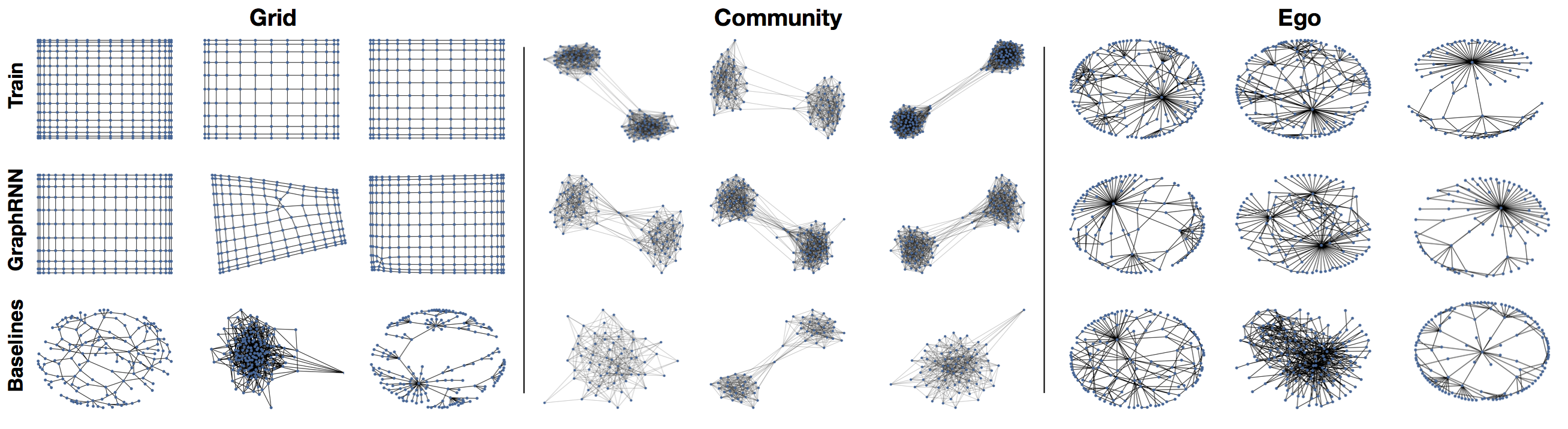
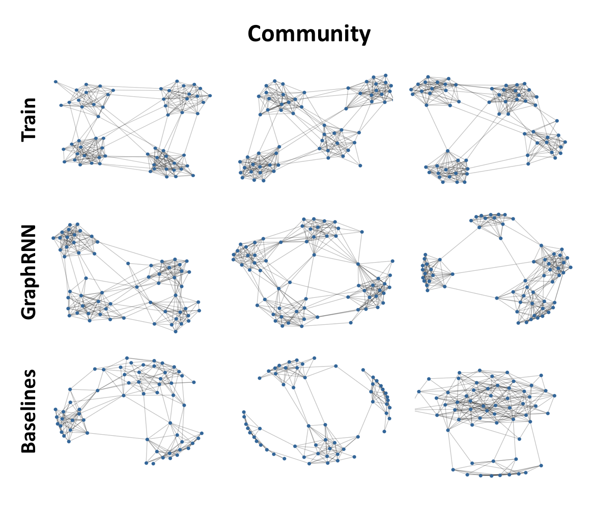
Graph visualization. Figure 2 visualizes the graphs generated by GraphRNN and various baselines, showing that GraphRNN can capture the structure of datasets with vastly differing characteristics—being able to effectively learn regular structures like grids as well as more natural structures like ego networks. Specifically, we found that grids generated by GraphRNN \ do not appear in the training set, i.e., it learns to generalize to unseen grid widths/heights.

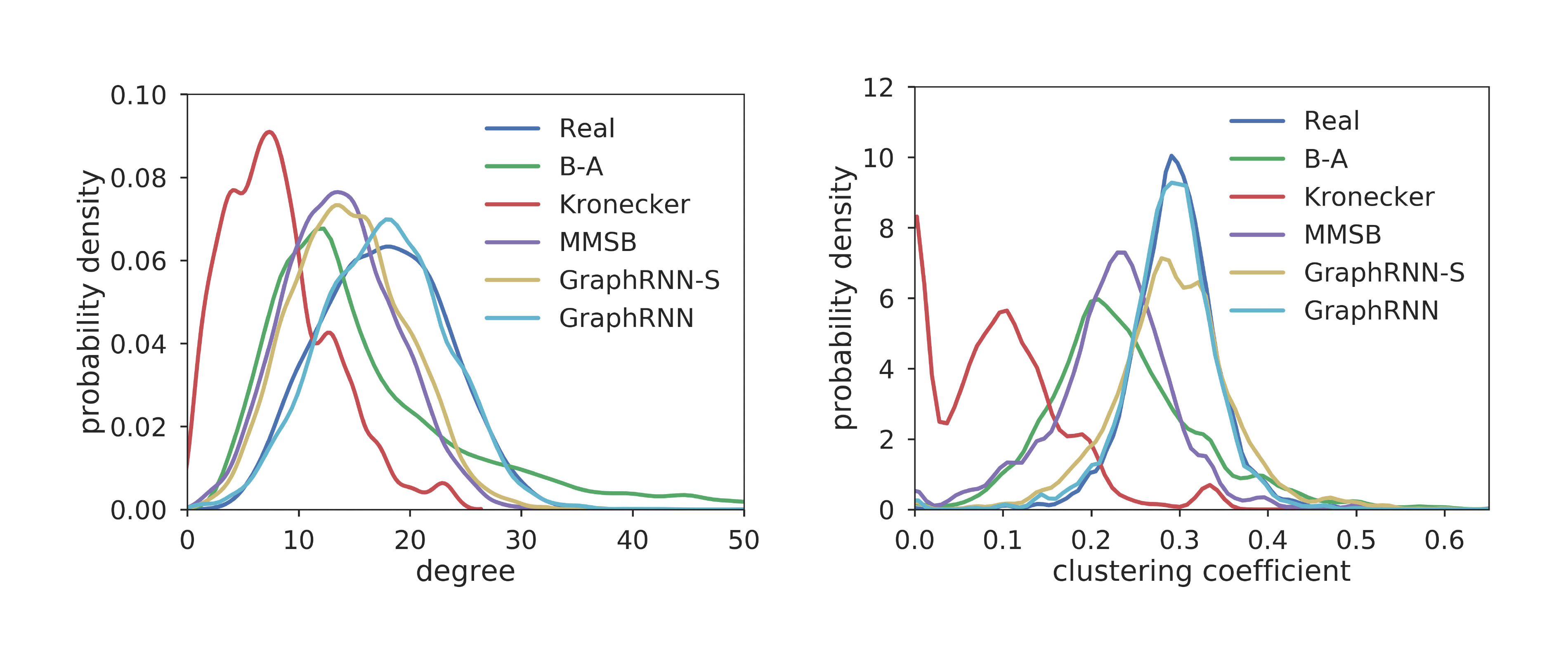
Evaluation with graph statistics. We use three graph statistics—based on degrees, clustering coefficients and orbit counts—to further quantitatively evaluate the generated graphs. Figure 3 shows the average graph statistics in the test vs. generated graphs, which demonstrates that even from hundreds of graphs with diverse sizes, GraphRNN can still learn to capture the underlying graph statistics very well, with the generated average statistics closely matching the overall test set distribution.

Table 1 and Table 2 summarize MMD evaluations on the full datasets and small versions, respectively. Note that we train all the models with a fixed number of steps, and report the test set performance at the step with the lowest training error.[^6] GraphRNN variants achieve the best performance on all datasets, with $80%$ decrease of MMD on average compared with traditional baselines, and $90%$ decrease of MMD compared with deep learning baselines. Interestingly, on the protein dataset, our simpler GraphRNN-S model performs very well, which is likely due to the fact that the protein dataset is a nearest neighbor graph over Euclidean space and thus does not involve highly complex edge dependencies. Note that even though some baseline models perform well on specific datasets (e.g., MMSB on the community dataset), they fail to generalize across other types of input graphs.

[^6]: Using the training set or a validation set to evaluate MMD gave analogous results, so we used the train set for early stopping.

Generalization ability. Table 2 also shows negative log-likelihoods (NLLs) on the training and test sets. We report the average $p(S^\pi)$ in our model, and report the likelihood in baseline methods as defined in their papers. A model with good generalization ability should have small NLL gap between training and test graphs. We found that our model can generalize well, with $22%$ smaller average NLL gap.[^7]

[^7]: The average likelihood is ill-defined for the traditional models.

4.5 Robustness

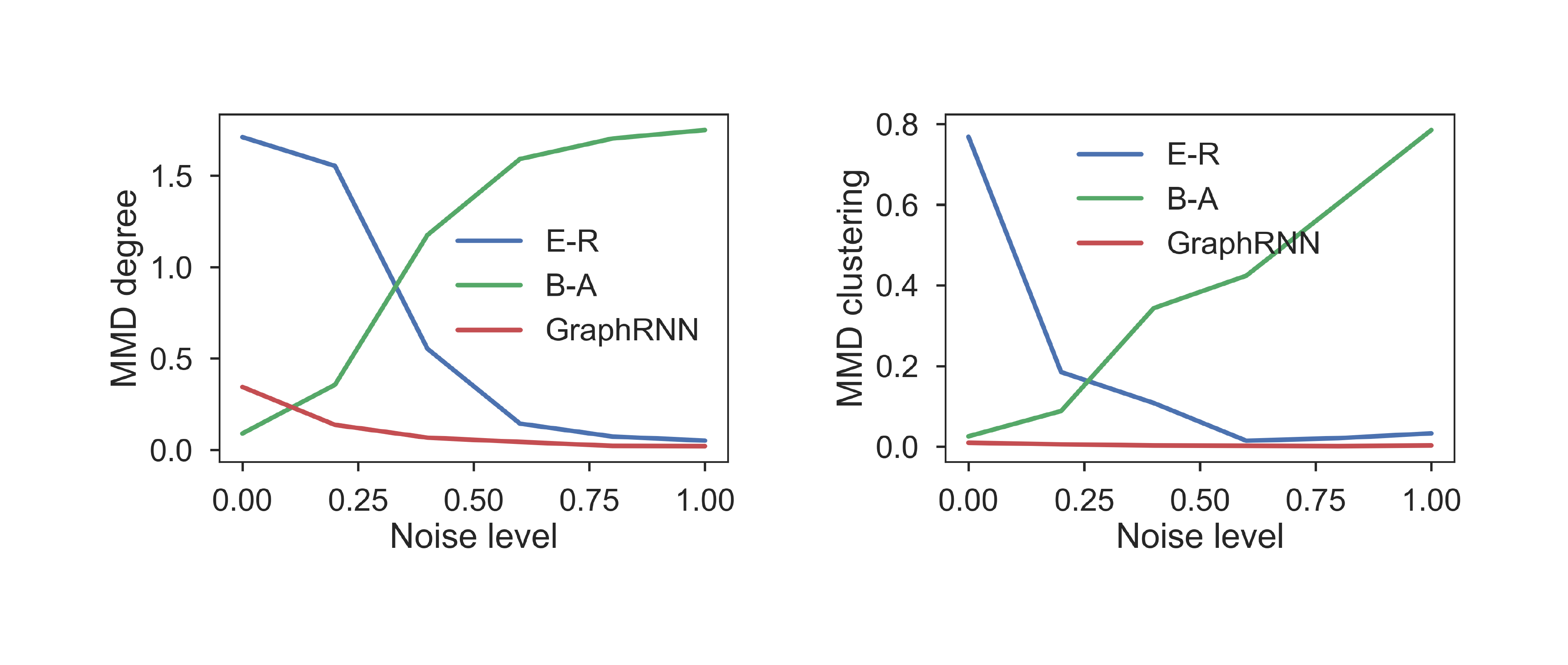
Finally, we also investigate the robustness of our model by interpolating between Barabási-Albert (B-A) and Erdős-Rényi (E-R) graphs. We randomly perturb [$0%, 20%, ..., 100%$] edges of B-A graphs with $100$ nodes. With $0%$ edges perturbed, the graphs are E-R graphs; with $100%$ edges perturbed, the graphs are B-A graphs. Figure 4 shows the MMD scores for degree and clustering coefficient distributions for the $6$ sets of graphs. Both B-A and E-R perform well when graphs are generated from their respective distributions, but their performance degrades significantly once noise is introduced. In contrast, GraphRNN maintains strong performance as we interpolate between these structures, indicating high robustness and versatility.

5. Further Related Work

Section Summary: This section discusses additional research that influenced the framework, beyond earlier surveys on graph generation methods. It highlights domain-specific efforts in generating molecules and parse trees for language processing, often using specialized formats like SMILES strings or grammar-based techniques, but notes that the current approach handles general graphs without such assumptions. It also draws from deep autoregressive models, which break down complex probabilities into simpler steps and have succeeded in images and audio, extending this to scalable graph generation that outperforms prior methods in handling broad graph types efficiently.

In addition to the deep graph generative approaches and traditional graph generation approaches surveyed previously, our framework also builds off a variety of other methods.

Molecule and parse-tree generation. There has been related domain-specific work on generating candidate molecules and parse trees in natural language processing. Most previous work on discovering molecule structures make use of a expert-crafted sequence representations of molecular graph structures (SMILES) [25, 26, 27]. Most recently, SD-VAE [28] introduced a grammar-based approach to generate structured data, including molecules and parse trees. In contrast to these works, we consider the fully general graph generation setting without assuming features or special structures of graphs.

Deep autoregressive models. Deep autoregressive models decompose joint probability distributions as a product of conditionals, a general idea that has achieved striking successes in the image [29] and audio [30] domains. Our approach extends these successes to the domain of generating graphs. Note that the DeepGMG algorithm [13] and the related prior work of [31] can also be viewed as deep autoregressive models of graphs. However, unlike these methods, we focus on providing a scalable (i.e., $O(n^2)$) algorithm that can generate general graphs.

6. Conclusion and Future Work

Section Summary: The researchers introduced GraphRNN, a new type of AI model that generates data structured like networks or graphs, and they created a thorough testing system to evaluate it. Their model outperformed earlier top-performing ones, handling large amounts of data efficiently and resisting errors well. Still, bigger hurdles exist, like expanding it to even larger networks and making it better at creating graphs based on specific conditions.

We proposed GraphRNN, an autoregressive generative model for graph-structured data, along with a comprehensive evaluation suite for the graph generation problem, which we used to show that GraphRNN achieves significantly better performance compared to previous state-of-the-art models, while being scalable and robust to noise. However, significant challenges remain in this space, such as scaling to even larger graphs and developing models that are capable of doing efficient conditional graph generation.

7. Acknowledgements

Section Summary: The authors express gratitude to Ethan Steinberg, Bowen Liu, Marinka Zitnik, and Srijan Kumar for their valuable discussions and feedback on the paper. The research received partial funding from organizations including DARPA SIMPLEX, ARO MURI, the Stanford Data Science Initiative, Huawei, JD, and the Chan Zuckerberg Biohub. Additionally, W.L.H. was supported by the SAP Stanford Graduate Fellowship and an NSERC PGS-D grant.

The authors thank Ethan Steinberg, Bowen Liu, Marinka Zitnik and Srijan Kumar for their helpful discussions and comments on the paper. This research has been supported in part by DARPA SIMPLEX, ARO MURI, Stanford Data Science Initiative, Huawei, JD, and Chan Zuckerberg Biohub. W.L.H. was also supported by the SAP Stanford Graduate Fellowship and an NSERC PGS-D grant.

Appendix

Section Summary: The appendix provides detailed implementation notes for the GraphRNN model, including two versions with different sizes for various datasets, using layered GRU recurrent neural networks for generating graph structures, and a simplified variant that performs similarly. It explains data preparation through random sampling and breadth-first search ordering to efficiently encode connections, along with training using the Adam optimizer over many iterations on a single GPU, which takes 12 to 24 hours for large datasets like proteins but generates new graphs in about one second. Additionally, it illustrates how GraphRNN captures the patterns in regular graph structures, such as grids or ladders, by relying on sequential edge predictions informed by prior connections to ensure valid formations.

A.1 Implementation Details of GraphRNN

In this section we detail parameter setting, data preparation and training strategies for GraphRNN.

We use two sets of model parameters for GraphRNN. One larger model is used to train and test on the larger datasets that are used to compare with traditional methods. One smaller model is used to train and test on datasets with nodes up to $20$. This model is only used to compare with the two most recent preliminary deep generative models for graphs proposed in [13, 12].

For GraphRNN, the graph-level RNN uses $4$ layers of GRU cells, with $128$ dimensional hidden state for the larger model, and $64$ dimensional hidden state for the smaller model in each layer. The edge-level RNN uses $4$ layers of GRU cells, with $16$ dimensional hidden state for both the larger model and the smaller model. To output the adjacency vector prediction, the edge-level RNN first maps the highest layer of the $16$ dimensional hidden state to a $8$ dimensional vector through a MLP with ReLU activation, then another MLP maps the vector to a scalar with sigmoid activation. The edge-level RNN is initialized by the output of the graph-level RNN at the start of generating $S^\pi_i$, $\forall 1 \le i \le n$. Specifically, the highest layer hidden state of the graph-level RNN is used to initialize the lowest layer of edge-level RNN, with a liner layer to match the dimensionality. During training time, teacher forcing is used for both graph-level and edge-level RNNs, i.e., we use the groud truth rather than the model's own prediction during training. At inference time, the model uses its own preditions at each time steps to generate a graph.

For the simple version GraphRNN-S, a two-layer MLP with ReLU and sigmoid activations respectively is used to generate $S^\pi_i$, with $64$ dimensional hidden state for the larger model, and $32$ dimensional hidden state for the smaller model. In practice, we find that the performance of the model is relatively stable with respect to these hyperparameters.

We generate the graph sequences used for training the model following the procedure in Section 2.3.4. Specifically, we first randomly sample a graph from the training set, then randomly permute the node ordering of the graph. We then do the deterministic BFS discussed in Section 2.3.4 over the graph with random node ordering, resulting a graph with BFS node ordering. An exception is in the robustness section, where we use the node ordering that generates B-A graphs to get graph sequences, in order to see if GraphRNN can capture the underlying preferential attachment properties of B-A graphs.

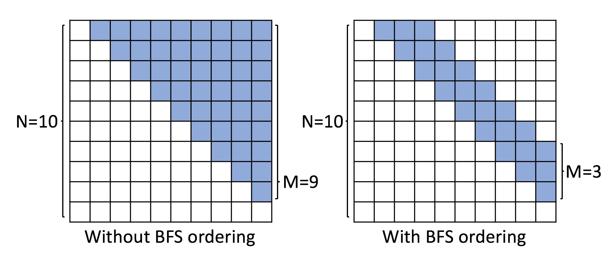
With the proposed BFS node ordering, we can reduce the maximum dimension $M$ of $S^\pi_i$, illustrated in Figure 5. To set the maximum dimension $M$ of $S^\pi_i$, we use the following empirical procedure. We randomly ran $100000$ times the above data pre-processing procedure to get graph with BFS node orderings. We remove the all consecutive zeros in all resulting $S^\pi_i$, to find the empirical distribution of the dimensionality of $S^\pi_i$. We set $M$ to be roughly the $99.9$ percentile, to account for the majority dimensionality of $S^\pi_i$. In principle, we find that graphs with regular structures tend to have smaller $M$, while random graphs or community graphs tend to have larger $M$. Specifically, for community dataset, we set $M=100$; for grid dataset, we set $M=40$; for B-A dataset, we set $M=130$; for protein dataset, we set $M=230$; for ego dataset, we set $M=250$; for all small graph datasets, we set $M=20$.

The Adam Optimizer is used for minibatch training. Each minibatch contains $32$ graph sequences. We train the model for $96000$ batchs in all experiments. We set the learning rate to be $0.001$, which is decayed by $0.3$ at step $12800$ and $32000$ in all experiments.

A.2 Running Time of GraphRNN

Training is performed on only $1$ Titan X GPU. For the protein dataset that consists of about $1000$ graphs, each containing about $500$ nodes, training converges at around $64000$ iterations. The runtime is around $12$ to $24$ hours. This also includes pre-processing, batching and BFS, which are currently implemented using CPU without multi-threading. The less expressive GraphRNN-S variant is about twice faster. At inference time, for the above dataset, generating a graph using the trained model only takes about $1$ second.

A.3 More Details on GraphRNN's Expressiveness

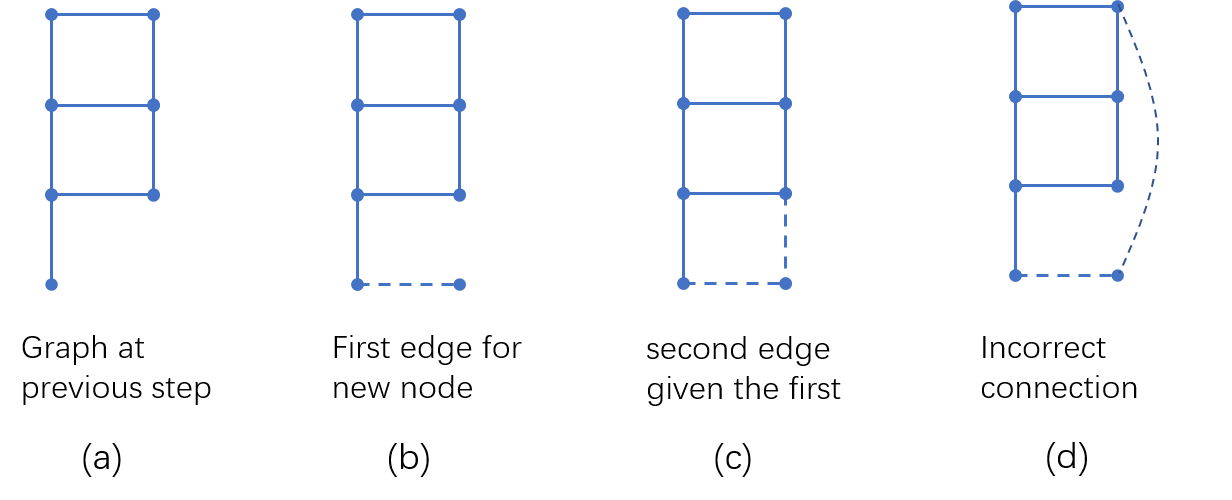
We illustrate the intuition underlying the good performance of GraphRNN on graphs with regular structures, such as grid and ladder networks. Figure 6 (a) shows the generation process of a ladder graph at an intermediate step. At this time step, the ground truth data (under BFS node ordering) specifies that the new node added to the graph should make an edge to the node with degree $1$. Note that node degree is a function of $S^\pi_{<i}$, thus could be approximated by a neural network.

Once the first edge has been generated, the new node should make an edge with another node of degree $2$. However, there are multiple ways to do so, but only one of them gives a valid grid structure, i.e. one that forms a $4$-cycle with the new edge. GraphRNN crucially relies on the edge-level RNN and the knowledge of the previously added edge, in order to distinguish between the correct and incorrect connections in Figure 6 (c) and (d).

A.4 Code Overview

In the code repository, main.py consists of the main training pipeline, which loads datasets and performs training and inference. It also consists of the Args class, which stores the hyper-parameter settings of the model. model.py consists of the RNN, MLP and loss function modules that are use to build GraphRNN. data.py contains the minibatch sampler, which samples a random BFS ordering of a batch of randomly selected graphs. evaluate.py contains the code for evaluating the generated graphs using the MMD metric introduced in Sec. 4.3.

Baselines including the Erdős-Rényi model, Barabási-Albert model, MMSB, and rge very recent deep generative models (GraphVAE, DeepGMG) are also implemented in the baselines folders. We adopt the C++ Kronecker graph model implementation in the SNAP package [^8].

[^8]: The SNAP package is available at http://snap.stanford.edu/snap/index.html.

A.5 Proofs

A.5.1 Proof of Proposition 1

We use the following observation:

########## {caption="\textbf{Observation 4"}

By definition of BFS, if $i < k$, then the children of $v_i$ in the BFS ordering come before the children of $v_k$ that do not connect to $v_{i'}$, $\forall 1 \le i' \le i$.

By definition of BFS, all neighbors of a node $v_i$ include the parent of $v_i$ in the BFS tree, all children of $v_i$ which have consecutive indices, and some children of $v_{i'}$ which connect to both $v_{i'}$ and $v_i$, for some $1 \le i' \le i$. Hence if $(v_i, v_{j-1}) \in E$ but $(v_i, v_j) \not \in E$, $v_{j-1}$ is the last children of $v_i$ in the BFS ordering. Hence $(v_{i}, v_{j'}) \not \in E$, $\forall j \le j' \le n$.

For all $i' \in [i]$, supposed that $(v_{i'}, v_{j'-1}) \in E$ but $(v_{i'}, v_{j'}) \not \in E$. By \textbf{Observation 4, $j' < j$. By conclusion in the previous paragraph, $(v_{i'}, v_{j''}) \not \in E$, $\forall j' \le j'' \le n$. Specifically, $(v_{i'}, v_{j''}) \not \in E$, $\forall j \le j'' \le n$. This is true for all $i' \in [i]$. Hence we prove that $(v_{i'}, v_{j'}) \not \in E$, $\forall 1 \le i' \le i$ and $j \le j' < n$.

A.5.2 Proof of Proposition 2

As proven in [?], this Wasserstein distance based kernel is a positive definite (p.d.) kernel. By properties that linear combinations, product and limit (if exists) of p.d. kernels are p.d. kernels, $k_W(p, q)$ is also a p.d. kernel.[^9] By the Moore-Aronszajn theorem, a symmetric p.d. kernel induces a unique RKHS. Therefore Equation (9) holds if we set $k$ to be $k_W$.

[^9]: This can be seen by expressing the kernel function using Taylor expansion.

A.6 Extension to Graphs with Node and Edge Features

Our GraphRNN model can also be applied to graphs where nodes and edges have feature vectors associated with them. In this extended setting, under node ordering $\pi$, a graph $G$ is associated with its node feature matrix $X^\pi\in\mathbb{R}^{n\times m}$ and edge feature matrix $F^\pi\in\mathbb{R}^{n\times k}$, where $m$ and $k$ are the feature dimensions for node and edge respectively. In this case, we can extend the definition of $S^\pi$ to include feature vectors of corresponding nodes as well as edges $S^\pi_i = (X^\pi_i, F^\pi_i)$. We can adapt the $f_{out}$ module, by using a MLP to generate $X^\pi_i$ and an edge-level RNN to genearte $F^\pi_i$ respectively. Note also that directed graphs can be viewed as an undirected graphs with two edge types, which is a special case under the above extension.

A.7 Extension to Graphs with Four Communities

To further show the ability of GraphRNN to learn from community graphs, we further conduct experiments on a four-community synthetic graph dataset. Specifically, the data set consists of 500 four community graphs with $48\leq|V|\leq68$. Each community is generated by the Erdős-Rényi model (E-R) [2] with $n \in [|V|/4-2, |V|/4+2]$ nodes and $p=0.7$. We then add $0.01|V|^2$ inter-community edges with uniform probability. Figure 7 shows the comparison of visualization of generated graph using GraphRNN and other baselines. We observe that in contrast to baselines, GraphRNN consistently generate 4-community graphs and each community has similar structure to that in the training set.

References

[1] Newman, M. Networks: an introduction. Oxford university press, 2010.

[2] Erdős, P. and Rényi, A. On random graphs I. Publicationes Mathematicae (Debrecen), 6:290–297, 1959.

[3] Leskovec, J., Chakrabarti, D., Kleinberg, J., Faloutsos, C., and Ghahramani, Z. Kronecker graphs: An approach to modeling networks. JMRL, 2010.

[4] Albert, R. and Barabási, L. Statistical mechanics of complex networks. Reviews of Modern Physics, 74(1):47, 2002.

[5] Airoldi, E., Blei, D., Fienberg, S., and Xing, E. Mixed membership stochastic blockmodels. JMLR, 2008.

[6] Leskovec, J., Kleinberg, J., and Faloutsos, C. Graph evolution: Densification and shrinking diameters. TKDD, 1(1):2, 2007.

[7] Robins, G., Pattison, P., Kalish, Y., and Lusher, D. An introduction to exponential random graph (p*) models for social networks. Social Networks, 29(2):173–191, 2007.

[8] Kingma, D. P. and Welling, M. Auto-encoding variational bayes. In ICLR, 2014.

[9] Goodfellow, I., Pouget-Abadie, J., Mirza, M., Xu, B., Warde-Farley, D., Ozair, S., Courville, A., and Bengio, Y. Generative adversarial nets. In NIPS, 2014.

[10] Kipf, T. N. and Welling, M. Variational graph auto-encoders. In NIPS Bayesian Deep Learning Workshop, 2016.

[11] Grover, A., Zweig, A., and Ermon, S. Graphite: Iterative generative modeling of graphs. In NIPS Bayesian Deep Learning Workshop, 2017.

[12] Simonovsky, M. and Komodakis, N. GraphVAE: Towards generation of small graphs using variational autoencoders, 2018. URL https://openreview.net/forum?id=SJlhPMWAW.

[13] Li, Y., Vinyals, O., Dyer, C., Pascanu, R., and Battaglia, P. Learning deep generative models of graphs, 2018. URL https://openreview.net/forum?id=Hy1d-ebAb.

[14] Cho, M., Sun, J., Duchenne, O., and Ponce, J. Finding matches in a haystack: A max-pooling strategy for graph matching in the presence of outliers. In CVPR, 2014.

[15] Gretton, A., Borgwardt, K. M., Rasch, M. J., Schölkopf, B., and Smola, A. A kernel two-sample test. JMLR, 2012.

[16] Hamilton, W. L., Ying, R., and Leskovec, J. Representation learning on graphs: Methods and applications. IEEE Data Engineering Bulletin, 2017.

[17] Chung, J., Gulcehre, C., Cho, K., and Bengio, Y. Empirical evaluation of gated recurrent neural networks on sequence modeling. NIPS Workshop on Deep Learning, 2014.

[18] Hornik, K. Approximation capabilities of multilayer feedforward networks. Neural networks, 4(2):251–257, 1991.

[19] Noy, M. and Ribó, A. Recursively constructible families of graphs. Advances in Applied Mathematics, 32(1-2):350–363, 2004.

[20] Dobson, P. and Doig, A. Distinguishing enzyme structures from non-enzymes without alignments. Journal of Molecular Biology, 330(4):771–783, 2003.

[21] Sen, P., Namata, G., Bilgic, M., Getoor, L., Galligher, B., and Eliassi-Rad, T. Collective classification in network data. AI Magazine, 29(3):93, 2008.

[22] Theis, L., van den Oord, A., and Bethge, M. A note on the evaluation of generative models. In ICLR, 2016.

[23] Lin, C. Hardness of approximating graph transformation problem. In International Symposium on Algorithms and Computation, 1994.

[24] Hočevar, T. and Demšar, J. A combinatorial approach to graphlet counting. Bioinformatics, 30(4):559–565, 2014.

[25] Olivecrona, M., Blaschke, T., Engkvist, O., and Chen, H. Molecular de novo design through deep reinforcement learning. Journal of Cheminformatics, 9(1):48, 2017.

[26] Segler, M., Kogej, T., Tyrchan, C., and Waller, M. Generating focussed molecule libraries for drug discovery with recurrent neural networks. ACS Central Science, 2017.

[27] Gómez-Bombarelli, R., Wei, J., Duvenaud, D., Hernández-Lobato, J. M., Sánchez-Lengeling, B., Sheberla, D., Aguilera-Iparraguirre, J., Hirzel, T. D., Adams, R. P., and Aspuru-Guzik, A. Automatic chemical design using a data-driven continuous representation of molecules. ACS Central Science, 2016.

[28] Dai, H., Tian, Y., Dai, B., Skiena, S., and Song, L. Syntax-directed variational autoencoder for structured data. ICLR, 2018.

[29] Oord, A., Kalchbrenner, N., and Kavukcuoglu, K. Pixel recurrent neural networks. In ICML, 2016b.

[30] Oord, A., Dieleman, S., Zen, H., Simonyan, K., Vinyals, O., Graves, A., Kalchbrenner, N., Senior, A., and Kavukcuoglu, K. Wavenet: A generative model for raw audio. arXiv preprint arXiv:1609.03499, 2016a.

[31] Johnson, D. D. Learning graphical state transitions. In ICLR, 2017.