Rigging the Lottery: Making All Tickets Winners
Utku Evci ${}^{1}$
Trevor Gale ${}^{1}$
Jacob Menick ${}^{2}$
Pablo Samuel Castro ${}^{1}$
Erich Elsen ${}^{2}$
${}^{1}$ Google Brain
${}^{2}$ DeepMind
Correspondence to: Utku Evci [email protected], Erich Elsen [email protected].
Proceedings of the 37th International Conference on Machine Learning, Vienna, Austria, PMLR 119, 2020. Copyright 2020 by the author(s).
Abstract
Many applications require sparse neural networks due to space or inference time restrictions. There is a large body of work on training dense networks to yield sparse networks for inference, but this limits the size of the largest trainable sparse model to that of the largest trainable dense model. In this paper we introduce a method to train sparse neural networks with a fixed parameter count and a fixed computational cost throughout training, without sacrificing accuracy relative to existing dense-to-sparse training methods. Our method updates the topology of the sparse network during training by using parameter magnitudes and infrequent gradient calculations. We show that this approach requires fewer floating-point operations (FLOPs) to achieve a given level of accuracy compared to prior techniques. We demonstrate state-of-the-art sparse training results on a variety of networks and datasets, including ResNet-50, MobileNets on Imagenet-2012, and RNNs on WikiText-103. Finally, we provide some insights into why allowing the topology to change during the optimization can overcome local minima encountered when the topology remains static[^1].
[^1]: Code available at github.com/google-research/rigl
Executive Summary: Neural networks, the core technology behind many AI applications like image recognition and language processing, often require vast computational resources, making them impractical for devices with limited space or power, such as smartphones or edge servers. Current approaches to creating smaller, "sparse" networks—ones that use far fewer active parameters—typically start by training a full-sized model and then trimming it, which wastes resources and caps the size of trainable models at what dense networks can handle. This inefficiency limits AI deployment in real-world scenarios where speed and efficiency are critical, especially as models grow larger to improve performance.
This document introduces RigL, a new algorithm designed to train sparse neural networks directly from a random starting point, keeping the number of parameters and the computational cost fixed and low throughout the process, while matching or exceeding the accuracy of traditional methods. The goal is to demonstrate that sparse networks can be trained efficiently without the overhead of dense training, potentially enabling bigger and better models.
The authors developed RigL by starting with a randomly sparsified network and periodically updating its structure: low-magnitude parameters are pruned, and new ones are added based on gradient signals that promise the fastest loss reduction. These updates occur infrequently to minimize extra computation. They tested RigL on standard benchmarks, including image classification on ImageNet-2012 and CIFAR-10 using convolutional networks like ResNet-50 and MobileNets, and language modeling on WikiText-103 with recurrent networks. Experiments used common training setups over thousands of steps, with sparsity levels from 50% to 96.5%, and compared against baselines like iterative pruning, static sparse training, and other dynamic methods. Key assumptions include uniform or scaled sparsity across layers to balance capacity and efficiency.
RigL's strongest results show it outperforms prior sparse training techniques, achieving up to 2-3% higher accuracy on ImageNet for 80-90% sparse ResNet-50 models while using 20-50% fewer floating-point operations (FLOPs) during training. At extreme sparsity, a 96.5% sparse ResNet-50 reached 72.75% top-1 accuracy—3.5% better than pruning—after extended training. Sparse MobileNets trained with RigL matched or exceeded dense versions with equivalent parameters, gaining 4.3% accuracy on ImageNet by scaling up width in sparse form. On CIFAR-10, 50% sparse networks sometimes beat the dense baseline by 0.5-1%, highlighting sparsity's regularization benefits. Finally, RigL's dynamic updates help models escape poor optimization traps, unlike fixed-topology methods that get stuck.
These findings mean organizations can build more accurate AI models with lower training and inference costs, reducing energy use and enabling deployment on resource-limited hardware. For instance, sparse models cut inference time by 50-90% without accuracy loss, impacting mobile apps, autonomous systems, and cloud efficiency. This challenges the view that sparsity always trades off performance, showing it can enhance it, especially for compact architectures like MobileNets. However, on language tasks, RigL lagged behind pruning by 5-10% in perplexity, suggesting task-specific tweaks are needed.
Leaders should prioritize RigL for projects needing efficient sparse models, starting with vision tasks where gains are clearest; integrate it into frameworks like TensorFlow for pilots on custom datasets. For broader use, invest in hardware accelerators that exploit sparsity to realize inference speedups. Future steps include refining RigL for recurrent networks via more data or hybrid approaches, and scaling to even larger models to test limits beyond current dense baselines.
While experiments are robust—repeated three times with code and checkpoints available—limitations include sensitivity to update schedules and sparsity distributions, which can double inference FLOPs in some cases. Language modeling results show gaps, possibly due to sequence dependencies. Confidence is high for image tasks (consistent outperformance across setups), but cautious for others until more validation.
1. Introduction
Section Summary: Sparse neural networks, which use fewer active connections to save on computation and memory, have proven efficient for tasks like image recognition and language processing, but current training methods often require the full resources of denser networks and can't create larger, more accurate models. This leads to inefficiencies, such as wasting effort on weights that end up zero, and leaves open questions about whether better sparse performance is possible. The paper introduces RigL, a new technique called the "Rigged Lottery" that trains sparse networks from scratch without needing a special starting point, achieving higher accuracy at lower costs than previous approaches while dynamically adjusting connections based on weights and gradients.
The parameter and floating point operation (FLOP) efficiency of sparse neural networks is now well demonstrated on a variety of problems ([1, 2]). Multiple works have shown inference time speedups are possible using sparsity for both Recurrent Neural Networks (RNNs) ([3]) and Convolutional Neural Networks (ConvNets) ([4, 5]). Currently, the most accurate sparse models are obtained with techniques that require, at a minimum, the cost of training a dense model in terms of memory and FLOPs ([6, 7]), and sometimes significantly more ([8]).
This paradigm has two main limitations. First, the maximum size of sparse models is limited to the largest dense model that can be trained; even if sparse models are more parameter efficient, we can't use pruning to train models that are larger and more accurate than the largest possible dense models. Second, it is inefficient; large amounts of computation must be performed for parameters that are zero valued or that will be zero during inference. Additionally, it remains unknown if the performance of the current best pruning algorithms is an upper bound on the quality of sparse models. [9] found that three different dense-to-sparse training algorithms all achieve about the same sparsity / accuracy trade-off. However, this is far from conclusive proof that no better performance is possible.
The Lottery Ticket Hypothesis ([10]) hypothesized that if we can find a sparse neural network with iterative pruning, then we can train that sparse network from scratch, to the same level of accuracy, by starting from the original initial conditions. In this paper we introduce a new method for training sparse models without the need of a "lucky" initialization; for this reason, we call our method "The Rigged Lottery" or RigL[^2]. We make the following specific contributions:
[^2]: Pronounced "wriggle".
- We introduce RigL - an algorithm for training sparse neural networks while maintaining memory and computational cost proportional to density of the network.
- We perform an extensive empirical evaluation of RigL on computer vision and natural language tasks. We show that RigL achieves higher quality than all previous techniques for a given computational cost.
- We show the surprising result that RigL can find more accurate models than the current best dense-to-sparse training algorithms.
- We study the loss landscape of sparse neural networks and provide insight into why allowing the topology of nonzero weights to change over the course of training aids optimization.
:Table 1: Comparison of different sparse training techniques. Drop and Grow columns correspond to the strategies used during the mask update. Selectable FLOPs is possible if the cost of training the model is fixed at the beginning of training.
| Method | Drop | Grow | Selectable FLOPs | Space & FLOPs $\propto$ |
|---|---|---|---|---|
| SNIP | $min(\vert\theta * \nabla_{\theta} L(\theta)\vert)$ | none | yes | sparse |
| DeepR | stochastic | random | yes | sparse |
| SET | $min(\vert\theta\vert)$ | random | yes | sparse |
| DSR | $min(\vert\theta\vert)$ | random | no | sparse |
| SNFS | $min(\vert\theta\vert)$ | momentum | no | dense |
| RigL (ours) | $min(\vert\theta\vert)$ | gradient | yes | sparse |
2. Related Work
Section Summary: Research on sparse neural networks began decades ago with techniques like magnitude-based pruning, where less important connections are removed and the network is retrained, evolving into more efficient methods such as gradual pruning over a single training round to reduce computational demands. Various alternative approaches, including regularization techniques and structured pruning that targets entire channels or neurons for faster performance, have been developed, with studies showing similar trade-offs in accuracy and sparsity across methods like L0 regularization and variational dropout. More recent advances focus on training sparse networks from the start using strategies like random rewiring, dynamic parameter shifting between layers, and momentum-based growth, alongside explorations of the Lottery Ticket Hypothesis, which suggests effective sparse subnetworks exist but may require specific initializations in large models.
Research on finding sparse neural networks dates back decades, at least to [11] who concluded that pruning weights based on magnitude was a simple and powerful technique. [12] later introduced the idea of retraining the previously pruned network to increase accuracy. [13] went further and introduced multiple rounds of magnitude pruning and retraining. This is, however, relatively inefficient, requiring ten rounds of retraining when removing $20%$ of the connections to reach a final sparsity of $90%$. To overcome this problem, [14] introduced gradual pruning, where connections are slowly removed over the course of a single round of training. [6] refined the technique to minimize the amount of hyper-parameter selection required.
A diversity of approaches not based on magnitude pruning have also been proposed. [15], [16] and [17] are some early examples, but impractical for modern neural networks as they use information from the Hessian to prune a trained network. More recent work includes $L_0$ Regularization ([18]), Variational Dropout ([8]), Dynamic Network Surgery ([7]), Discovering Neural Wirings ([19]), Sensitivity Driven Regularization ([20]). [9] examined magnitude pruning, $L_0$ Regularization, and Variational Dropout and concluded that they all achieve about the same accuracy versus sparsity trade-off on ResNet-50 and Transformer architectures.
There are also structured pruning methods which attempt to remove channels or neurons so that the resulting network is dense and can be accelerated easily ([21, 22, 18]). We compare RigL with these state-of-the-art structured pruning methods in Appendix B. We show that our method requires far fewer resources and finds smaller networks that require less FLOPs to run.
The first training technique to allow for sparsity throughout the entire training process was, to our knowledge, first introduced in Sparse Evolutionary Training (SET) ([23]). The weights are pruned according to the standard magnitude criterion used in pruning and are added back at random. The method is simple and achieves reasonable performance in practice. Following this, Deep Rewiring (DeepR) ([24]) augmented Stochastic Gradient Descent (SGD) with a random walk in parameter space. Additionally, at initialization connections are assigned a pre-defined sign at random; when the optimizer would normally flip the sign, the weight is set to 0 instead and new weights are activated at random.
Dynamic Sparse Reparameterization (DSR) ([25]) introduced the idea of allowing the parameter budget to shift between different layers of the model, allowing for non-uniform sparsity. This allows the model to distribute parameters where they are most effective. Unfortunately, the models under consideration are mostly convolutional networks, so the result of this parameter reallocation (which is to decrease the sparsity of early layers and increase the sparsity of later layers) has the overall effect of increasing the FLOP count because the spatial size is largest in the early layers. Sparse Networks from Scratch (SNFS) ([26]) introduces the idea of using the momentum of each parameter as the criterion to be used for growing weights and demonstrates it leads to an improvement in test accuracy. Like DSR, they allow the sparsity of each layer to change and focus on a constant parameter, not FLOP, budget. Importantly, the method requires computing gradients and updating the momentum for every parameter in the model, even those that are zero, at every iteration. This can result in a significant amount of overall computation. Additionally, depending on the model and training setup, the required storage for the full momentum tensor could be prohibitive. Single-Shot Network Pruning (SNIP) ([27]) attempts to find an initial mask with one-shot pruning and uses the saliency score of parameters to decide which parameters to keep. After pruning, training proceeds with this static sparse network. Properties of the different sparse training techniques are summarized in Table 1.
There has also been a line of work investigating the Lottery Ticket Hypothesis ([10]). [28] showed that the formulation must be weakened to apply to larger networks such as ResNet-50 ([29]). In large networks, instead of the original initialization, the values after thousands of optimization steps must be used for initialization. [30] showed that "winning lottery tickets" obtain non-random accuracies even before training has started. Though the possibility of training sparse neural networks with a fixed sparsity mask using lottery tickets is intriguing, it remains unclear whether it is possible to generate such initializations – for both masks and parameters – de novo.
3. Rigging The Lottery
Section Summary: RigL is a method for training sparse neural networks that begins with a randomly thinned-out network and periodically prunes weak connections based on their size while adding new ones guided by the strongest signals from the network's learning process. It distributes sparsity across layers using strategies like uniform reduction or patterns inspired by random graph models to keep the overall model efficient without resizing layers, and updates happen at set intervals with a decaying frequency to gradually refine the structure. The key innovation is selecting new connections from high-impact gradients and setting them to zero initially, allowing the network to adapt without disrupting ongoing training.
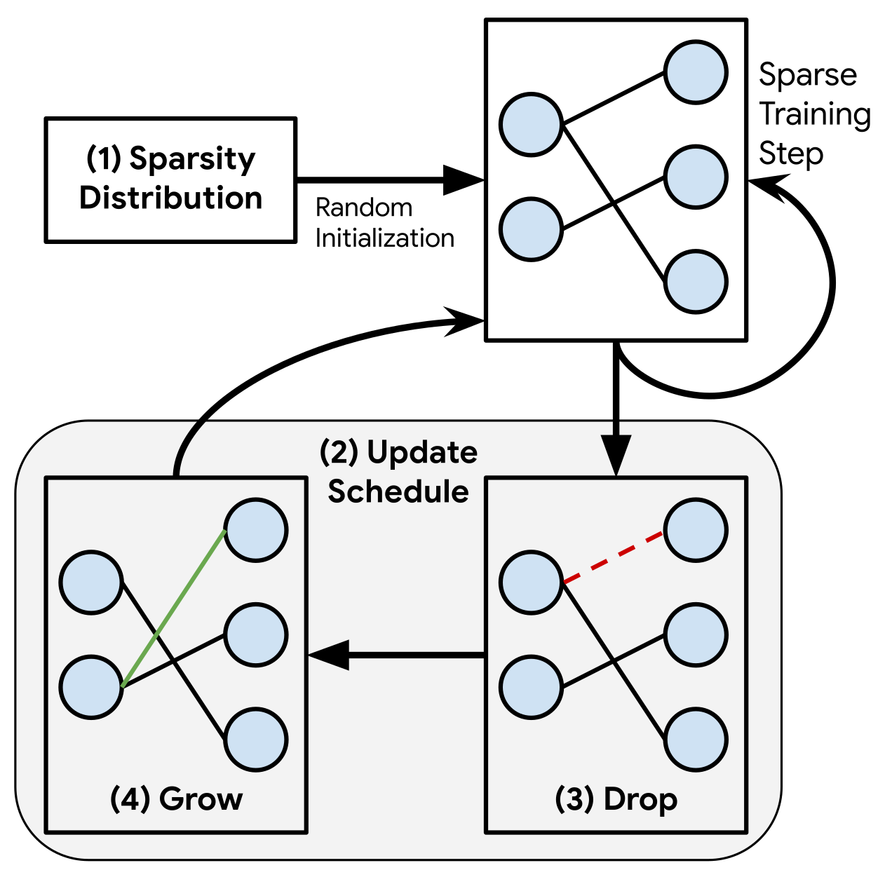
Our method, RigL, is illustrated in Figure 1 and detailed in Algorithm 1. RigL starts with a random sparse network, and at regularly spaced intervals it removes a fraction of connections based on their magnitudes and activates new ones using instantaneous gradient information. After updating the connectivity, training continues with the updated network until the next update. The main parts of our algorithm, Sparsity Distribution, Update Schedule, Drop Criterion, Grow Criterion, and the various options considered for each, are explained below.
(0) Notation. Given a dataset $D$ with individual samples $x_i$ and targets $y_i$, we aim to minimize the loss function $\sum_i L(f_{\Theta}(x_i), y_i)$, where $f_{\Theta}(\cdot)$ is a neural network with parameters $\Theta \in \mathbb{R}^N$. Parameters of the $l^{th}$ layer are denoted with $\Theta^l$ which is a length $N^l$ vector. A sparse layer drops a fraction $s^l \in (0, 1)$ of its connections and parameterized with vector $\theta^l$ of length $(1-s^l)N^l$. Parameters of the corresponding sparse network is denoted with $\theta$. Finally, the overall sparsity of a sparse network is defined as the ratio of zeros to the total parameter count, i.e. $S=\frac{\sum_l s^lN^l}{N}$
(1) Sparsity Distribution. There are many ways of distributing the non-zero weights across the layers while maintaining a certain overall sparsity. We avoid re-allocating parameters between layers during the training process as it makes it difficult to target a specific final FLOP budget, which is important for many applications. We consider the following three strategies:
- Uniform: The sparsity $s^l$ of each individual layer is equal to the total sparsity $S$. In this setting, we keep the first layer dense, since sparsifying this layer has a disproportional effect on the performance and almost no effect on the total size.
- Erdős-Rényi: As introduced in [23], $s^l$ scales with $1- \frac{n^{l-1}+n^{l}}{n^{l-1} * n^{l}}$, where $n^l$ denotes number of neurons at layer $l$. This enables the number of connections in a sparse layer to scale with the sum of the number of output and input channels.
- Erdős-Rényi-Kernel (ERK): This method modifies the original Erdős-Rényi formulation by including the kernel dimensions in the scaling factors. In other words, the number of parameters of the sparse convolutional layers are scaled proportional to $1- \frac{n^{l-1}+n^{l}+w^l+h^l}{n^{l-1} * n^{l}w^lh^l}$, where $w^l$ and $h^l$ are the width and the height of the $l$ 'th convolutional kernel. Sparsity of the fully connected layers scale as in the original Erdős-Rényi formulation. Similar to Erdős-Rényi, ERK allocates higher sparsities to the layers with more parameters while allocating lower sparsities to the smaller ones.
In all methods, the bias and batch-norm parameters are kept dense, since these parameters scale with total number of neurons and have a negligible effect on the total model size.
(2) Update Schedule. The update schedule is defined by the following parameters: (1) $\Delta T$: the number of iterations between sparse connectivity updates, (2) $T_{end}$: the iteration at which to stop updating the sparse connectivity, (3) $\alpha$: the initial fraction of connections updated and (4) $f_{decay}$: a function, invoked every $\Delta T$ iterations until $T_{end}$, possibly decaying the fraction of updated connections over time. For the latter, as in [26], we use cosine annealing, as we find it slightly outperforms the other methods considered.
$ f_{decay}(t;~\alpha, ~T_{end})=\frac{\alpha}{2}\left(1+cos\left(\frac{t\pi}{T_{end}}\right)\right) $
Results obtained with other annealing functions, such as constant and inverse power, are presented in Appendix G.
(3) Drop criterion. Every $\Delta T$ steps we drop the connections given by $ArgTopK(-|\theta^l|, f_{decay}(t;~\alpha, T_{end})(1-s^l) N^l)$, where $ArgTopK(v, ~k)$ gives the indices of the top- $k$ elements of vector $v$.
(4) Grow criterion. The novelty of our method lies in how we grow new connections. We grow the connections with highest magnitude gradients, $ArgTopK_{i \notin \theta^l \setminus \mathbb{I}{active}}(|\nabla{\Theta^l} L_t|, ~k)$, where $\theta^l \setminus \mathbb{I}_{active}$ is the set of active connections remaining after step (3). Newly activated connections are initialized to zero and therefore don't affect the output of the network. However they are expected to receive gradients with high magnitudes in the next iteration and therefore reduce the loss fastest. We attempted using other initialization like random values or small values along the gradient direction for the activated connections, however these experiments didn't provide better results.
This procedure can be applied to each layer in sequence and the dense gradients can be discarded immediately after selecting the top connections. If a layer is too large to store the full gradient with respect to the weights, then the gradients can be calculated in an online manner and only the top-k gradient values are stored. As long as $\Delta T > \frac{1}{1-s}$, the extra work of calculating dense gradients is amortized and still proportional to $1-S$. This is in contrast to the method of [26], which requires calculating and storing the full gradients at each optimization step.
**Input:** Network $f_\Theta$, dataset $D$
Sparsity Distribution: $\mathbb{S}=\{s^1, \dots, s^L\}$
Update Schedule: $\Delta T$, $T_{end}$, $\alpha$, $f_{decay}$
$\theta \gets$ Randomly sparsify $\Theta$ using $\mathbb{S}$
**for** each training step $t$ **do**
  Sample a batch $B_t \sim D$
  $L_t =\sum_{i \sim B_t} L((f_{\theta}(x_i),~y_i) $
  **if** $t \ (\mathrm{mod}\ \Delta T)== 0$ and  $t < T_{end}$ **then**
    **for** each layer $l$ **do**
      $k = f_{decay}(t;~\alpha,T_{end})(1-s^l)N^l$
      $\mathbb{I}_{active} = ArgTopK(-|\theta^l|,~k)$
      $\mathbb{I}_{grow} = ArgTopK_{i \notin \theta^l \setminus \mathbb{I}_{active}}(|\nabla_{\Theta^l} L_t|,~k)$
      $\theta \gets$ Update connections $\theta$ using $\mathbb{I}_{active}$ and $\mathbb{I}_{grow}$
    **end for**
  **else**
    $\theta = \theta - \alpha \nabla_{\theta}L_t$
  **end if**
**end for**
4. Empirical Evaluation
Section Summary: The empirical evaluation section tests various sparse training methods for neural networks on image classification tasks using datasets like ImageNet-2012 and CIFAR-10, as well as language modeling on WikiText-103, with experiments repeated three times to ensure reliable results. It details setups like optimizer choices and training schedules, noting that dynamic methods such as RigL, SET, and SNFS benefit from extended training time, which scales up the steps and improves performance. Key results on ResNet-50 show RigL achieving the highest accuracy for sparse models—outperforming random growth approaches and even dense networks with similar parameters—while using fewer computational resources, with similar advantages seen in MobileNets.
Our experiments include image classification using CNNs on the ImageNet-2012 ([31]) and CIFAR-10 ([32]) datasets and character based language modeling using RNNs with the WikiText-103 dataset ([33]). We repeat all of our experiments 3 times and report the mean and standard deviation. We use the TensorFlow Model Pruning library ([6]) for our pruning baselines. A Tensorflow ([34]) implementation of our method along with three other baselines (SET, SNFS, SNIP) and checkpoints of our models can be found at github.com/google-research/rigl. You can also check the reproducibility report about our work at https://github.com/varun19299/rigl-reproducibility ([35]).
For all dynamic sparse training methods (SET, SNFS, RigL), we use the same update schedule with $\Delta T=100$ and $\alpha=0.3$ unless stated otherwise. Corresponding hyper-parameter sweeps can be found in Section 4.4. We set the momentum value of SNFS to 0.9 and investigate other values in Appendix D. We observed that stopping the mask updates prior to the end of training yields slightly better performance; therefore, we set $T_{end}$ to 25k for ImageNet-2012 and 75k for CIFAR-10 training which corresponds to roughly 3/4 of the full training.
The default number of training steps used for training dense networks might not be optimal for sparse training with dynamic connectivity. In our experiments we observe that sparse training methods benefit significantly from increased training steps. When increasing the training steps by a factor $M$, the anchor epochs of the learning rate schedule and the end iteration of the mask update schedule are also scaled by the same factor; we indicate this scaling with a subscript (e.g. RigL$_{M\times}$).
Additionally, in Appendix B, we compare RigL with structured pruning algorithms and in Appendix E we show that solutions found by RigL are not lottery tickets.
4.1 ImageNet-2012 Dataset
In all experiments in this section, we use SGD with momentum as our optimizer. We set the momentum coefficient of the optimizer to 0.9, $L_2$ regularization coefficient to 0.0001, and label smoothing ([36]) to 0.1. The learning rate schedule starts with a linear warm up reaching its maximum value of 1.6 at epoch 5 which is then dropped by a factor of 10 at epochs 30, 70 and 90. We train our networks with a batch size of 4096 for 32000 steps which roughly corresponds to 100 epochs of training. Our training pipeline uses standard data augmentation, which includes random flips and crops.
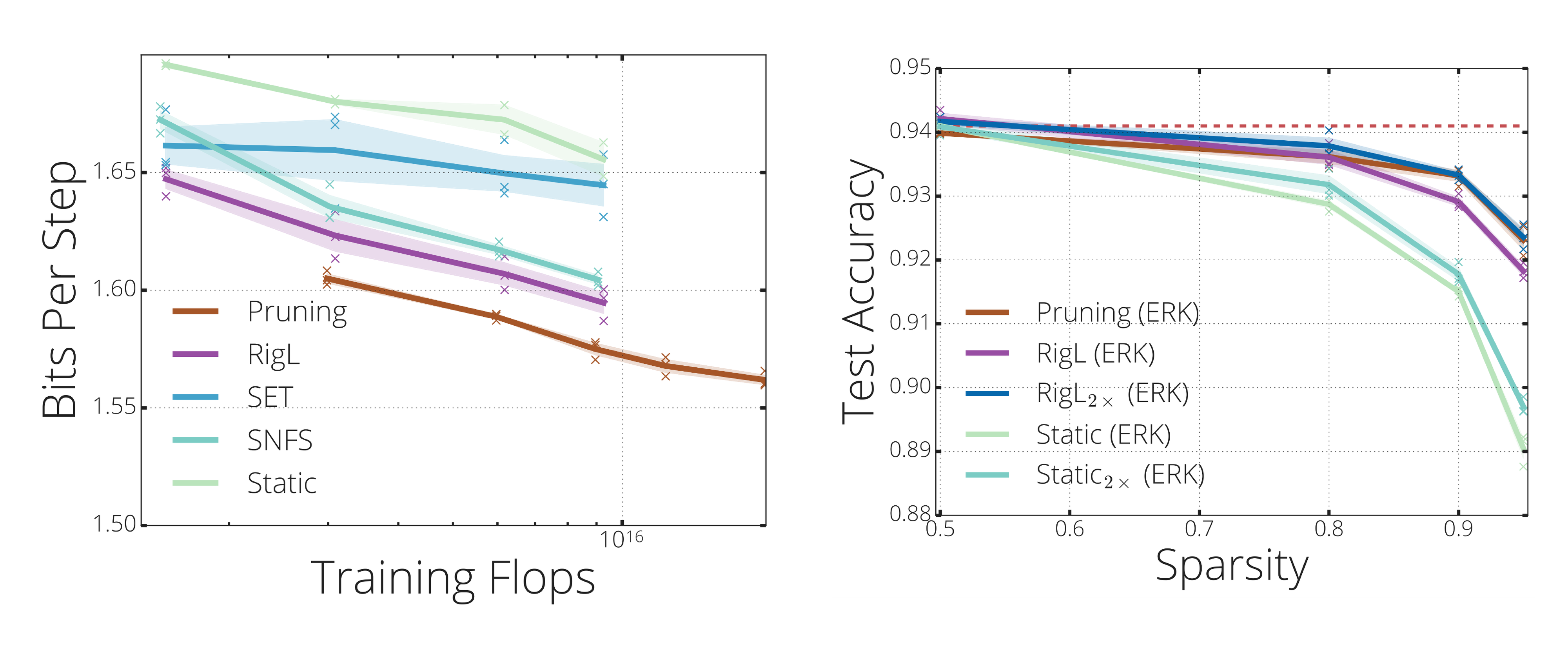
![**Figure 2:** **(left)** Performance and cost of training 80% and 90% sparse ResNet-50s on the Imagenet-2012 classification task. We report FLOPs needed for training and test (inference on single sample) and normalize them with the FLOPs of a dense model. To make a fair comparison we assume pruning algorithm utilizes sparsity during the training (see H for details on how FLOPs are calculated). Methods with superscript '*' indicates reported results in corresponding papers (except DNW results, which is obtained from ([37])). Pruning results are obtained from [9]. **(top-right)** Performance of sparse training methods on training 80% sparse ResNet-50 with uniform sparsity distribution. Points at each curve correspond to the individual training runs with training multipliers from 1 to 5 (except pruning which is scaled between 0.5 and 2). The number of FLOPs required to train a standard dense ResNet-50 along with its performance is indicated with a dashed red line. **(bottom-right)** Performance of *RigL* at different sparsity levels with extended training.](https://ittowtnkqtyixxjxrhou.supabase.co/storage/v1/object/public/public-images/rc2ep8ut/complex_fig_8715127d27a1.png)
4.1.1 ResNet-50
Figure 2-top-right summarizes the performance of various methods on training an 80% sparse ResNet-50. We also train small dense networks with equivalent parameter count. All sparse networks use a uniform layer-wise sparsity distribution unless otherwise specified and a cosine update schedule ($\alpha=0.3$, $\Delta T=100$). Overall, we observe that the performance of all methods improves with training time; thus, for each method we run extended training with up to 5 $\times$ the training steps of the original.
As noted by [9], [38], [28], and [25], training a network with fixed sparsity from scratch (Static) leads to inferior performance. Training a dense network with the same number of parameters (Small-Dense) gets better results than Static, but fails to match the performance of dynamic sparse models. SET improves the performance over Small-Dense, however saturates around 75% accuracy indicating the limits of growing new connections randomly. Methods that use gradient information to grow new connections (RigL and SNFS) obtain higher accuracies, but RigL achieves the highest accuracy and does so while consistently requiring fewer FLOPs than the other methods.
![**Figure 3:** **(left)** *RigL* significantly improves the performance of sparse MobileNets (v1 and v2) on ImageNet-2012 dataset and exceeds the *pruning* results reported by [6]. Performance of the dense MobileNets are indicated with red lines. **(right)** Performance of sparse MobileNet-v1 architectures presented with their inference FLOPs. Networks with *ERK* distribution get better performance with the same number of parameters but take more FLOPs to run. Training wider sparse models with *RigL* (*Big-Sparse*) yields a significant performance improvement over the dense model.](https://ittowtnkqtyixxjxrhou.supabase.co/storage/v1/object/public/public-images/rc2ep8ut/complex_fig_ff1a8b24b38d.png)
Given that different applications or scenarios might require a limit on the number of FLOPs for inference, we investigate the performance of our method at various sparsity levels. As mentioned previously, one strength of our method is that its resource requirements are constant throughout training and we can choose the level of sparsity that fits our training and/or inference constraints. In Figure 2-bottom-right we show the performance of our method at different sparsities and compare them with the pruning results of [9], which uses 1.5x training steps, relative to the original 32k iterations. To make a fair comparison with regards to FLOPs, we scale the learning schedule of all other methods by 5x. Note that even after extending the training, it takes less FLOPs to train sparse networks using RigL compared to the pruning method[^3].
[^3]: Except for the 80% sparse RigL-ERK
RigL, our method with constant sparsity distribution, exceeds the performance of magnitude based iterative pruning in all sparsity levels while requiring less FLOPs to train. Sparse networks that use Erdős-Renyi-Kernel (ERK) sparsity distribution obtains even greater performance. For example ResNet-50 with 96.5% sparsity achieves a remarkable 72.75% Top-1 Accuracy, around 3.5% higher than the extended magnitude pruning results reported by [9]. As observed earlier, smaller dense models (with the same number of parameters) or sparse models with a static connectivity can not perform at a comparable level.
A more fine grained comparison of sparse training methods is presented in Figure 2-left. Methods using uniform sparsity distribution and whose FLOP/memory footprint scales directly with (1-S) are placed in the first sub-group of the table. The second sub-group includes DSR and networks with ERK sparsity distribution which require a higher number of FLOPs for inference with same parameter count. The final sub-group includes methods that require the space and the work proportional to training a dense model.
4.1.2 MobileNet
MobileNet is a compact architecture that performs remarkably well in resource constrained settings. Due to its compact nature with separable convolutions it is known to be difficult to sparsify without compromising performance ([6]). In this section we apply our method to MobileNet-v1 ([39]) and MobileNet-v2 ([40]). Due to its low parameter count we keep the first layer and depth-wise convolutions dense. We use ERK or Uniform sparsity distributions to sparsify the remaining layers. We calculate sparsity fractions in this section over pruned layers and real sparsities (when first layer and depth-wise convolutions are included) are slightly lower than the reported values (i.e. 74.2, 84.1, 89, 94 for 75, 85, 90, 95 % sparsity).
The performance of sparse MobileNets trained with RigL as well as the baselines are shown in Figure 3. We extend the training (5x of the original number of steps) for all runs in this section. RigL trains 75% sparse MobileNets with no loss in performance. Performance starts dropping after this point, though RigL consistently gets the best results by a large margin.
Figure 2-top-right and Figure 3-left show that the sparse models are more accurate than the dense models with the same number of parameters, corroborating the results of [3]. To validate this point further, we train a sparse MobileNet-v1 with width multiplier of 1.98 and constant sparsity of 75%, which has the same FLOPs and parameter count as the dense baseline. Training this network with RigL yields an impressive 4.3% absolute improvement in Top-1 Accuracy demonstrating the exciting potential of sparse networks at increasing the performance of widely-used dense models.
4.2 Character Level Language Modeling
Most prior work has only examined sparse training on vision networks [^4]. To fully understand these techniques it is important to examine different architectures on different datasets. [3] found sparse GRUs ([41]) to be very effective at modeling speech, however the dataset they used is not available. We choose a proxy task with similar characteristics (dataset size and vocabulary size are approximately the same) - character level language modeling on the publicly available WikiText-103 ([33]) dataset.
[^4]: The exception being the work of [24]
Our network consists of a shared embedding with dimensionality 128, a vocabulary size of 256, a GRU with a state size of 512, a readout from the GRU state consisting of two linear layers with width 256 and 128 respectively. We train the next step prediction task with the cross entropy loss using the Adam optimizer. The remaining hyper-parameters are reported in Appendix I.
In Figure 4-left we report the validation bits per step of various solutions at the end of the training. For each method we perform extended runs to see how the performance of each method scales with increased training time. As observed before, SET performs worse than the other dynamic training methods and its performance improves only slightly with increased training time. On the other hand the performance of RigL and SNFS continuously improves with more training steps. Even though RigL exceeds the performance of the other sparse training approaches it fails to match the performance of pruning in this setting, highlighting an important direction for future work.
4.3 WideResNet-22-2 on CIFAR-10
We also evaluate the performance of RigL on the CIFAR-10 image classification benchmark. We train a Wide Residual Network ([42]) with 22 layers using a width multiplier of 2 for 250 epochs (97656 steps). The learning rate starts at 0.1 which is scaled down by a factor of 5 every 30, 000 iterations. We use an L2 regularization coefficient of 5e-4, a batch size of 128 and a momentum coefficient of 0.9. We use the default mask update interval for RigL ($\Delta T=100$) and the default ERK sparsity distribution. Results with other mask update intervals and sparsity distributions yield similar results. These can be found in Appendix J.
The final accuracy of RigL for various sparsity levels is presented in Figure 4-right. The dense baseline obtains 94.1% test accuracy; surprisingly, some of the 50% sparse networks generalize better than the dense baseline demonstrating the regularization aspect of sparsity. With increased sparsity, we see a performance gap between the Static and Pruning solutions. Training static networks longer seems to have limited effect on the final performance. On the other hand, RigL matches the performance of pruning with only a fraction of the resources needed for training.
4.4 Analyzing the performance of RigL
In this section we study the effect of sparsity distributions and update schedules on the performance of our method. The results for SET and SNFS are similar and are discussed in Appendix C and Appendix F. Additionally, we investigate the energy landscape of sparse ResNet-50s and show that dynamic connectivity provided by RigL helps escaping sub-optimal solutions found by static training.
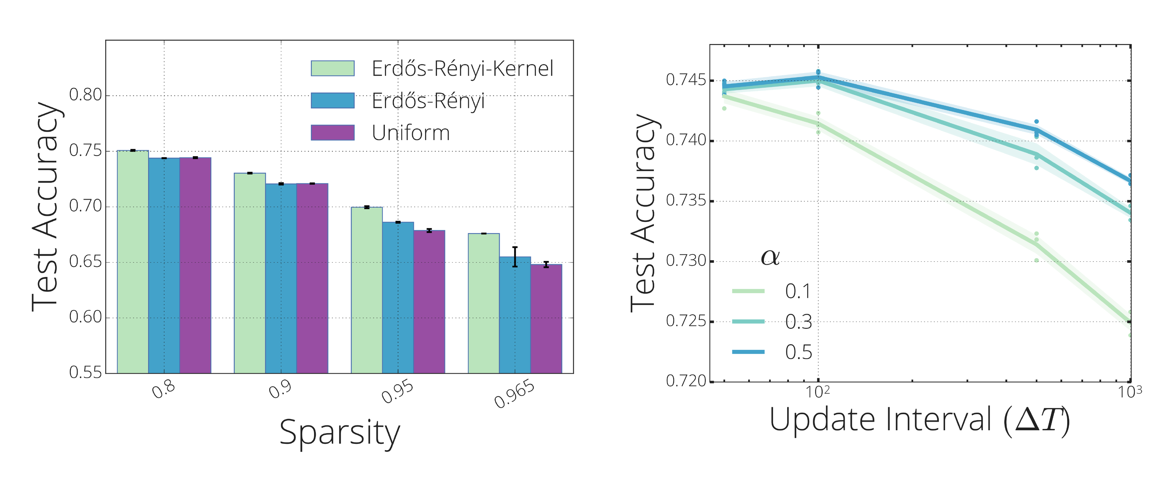
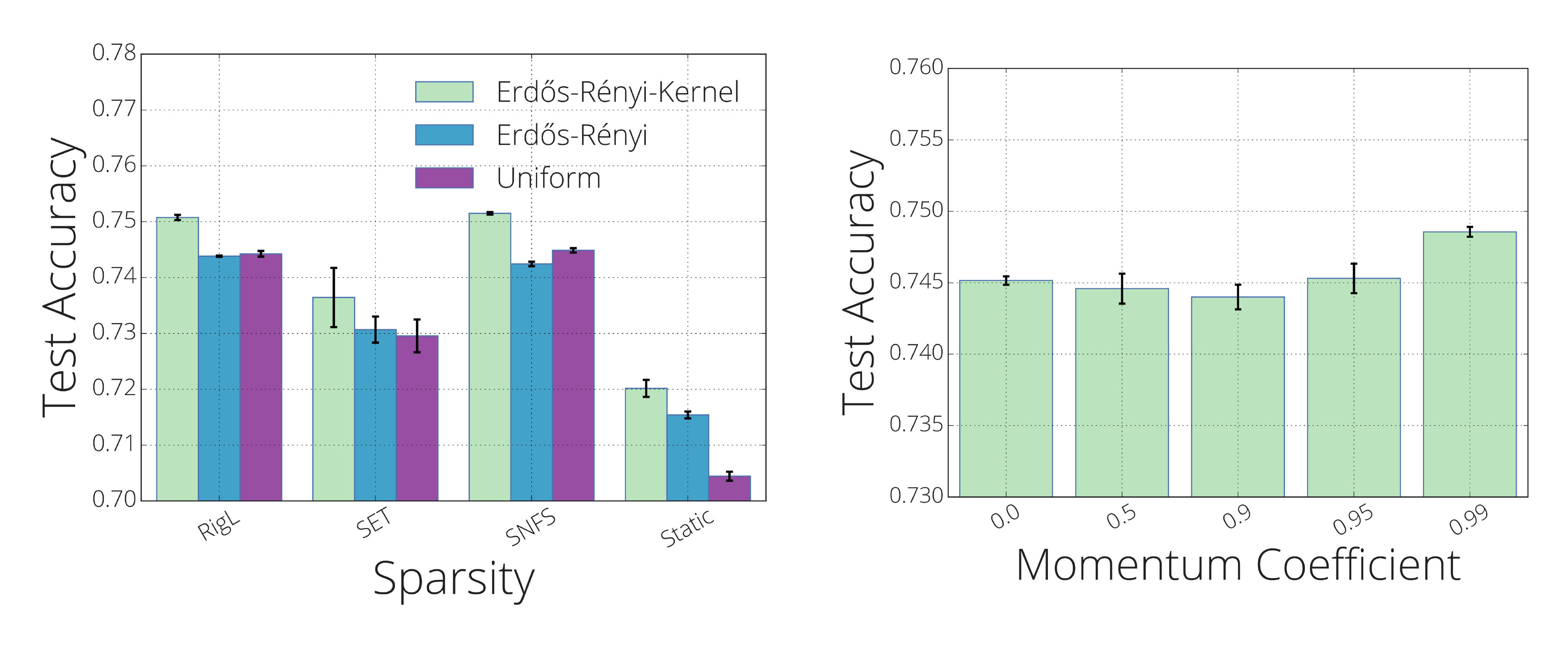
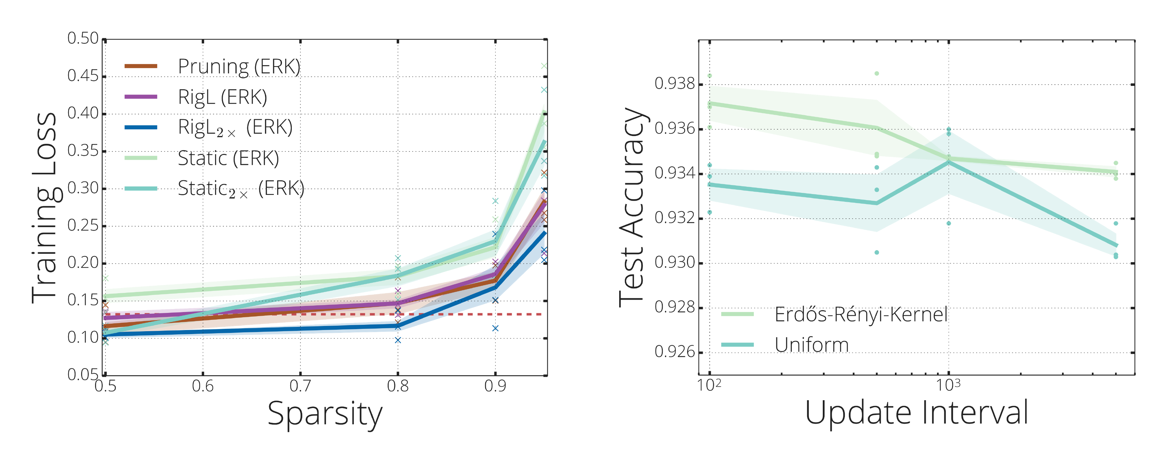
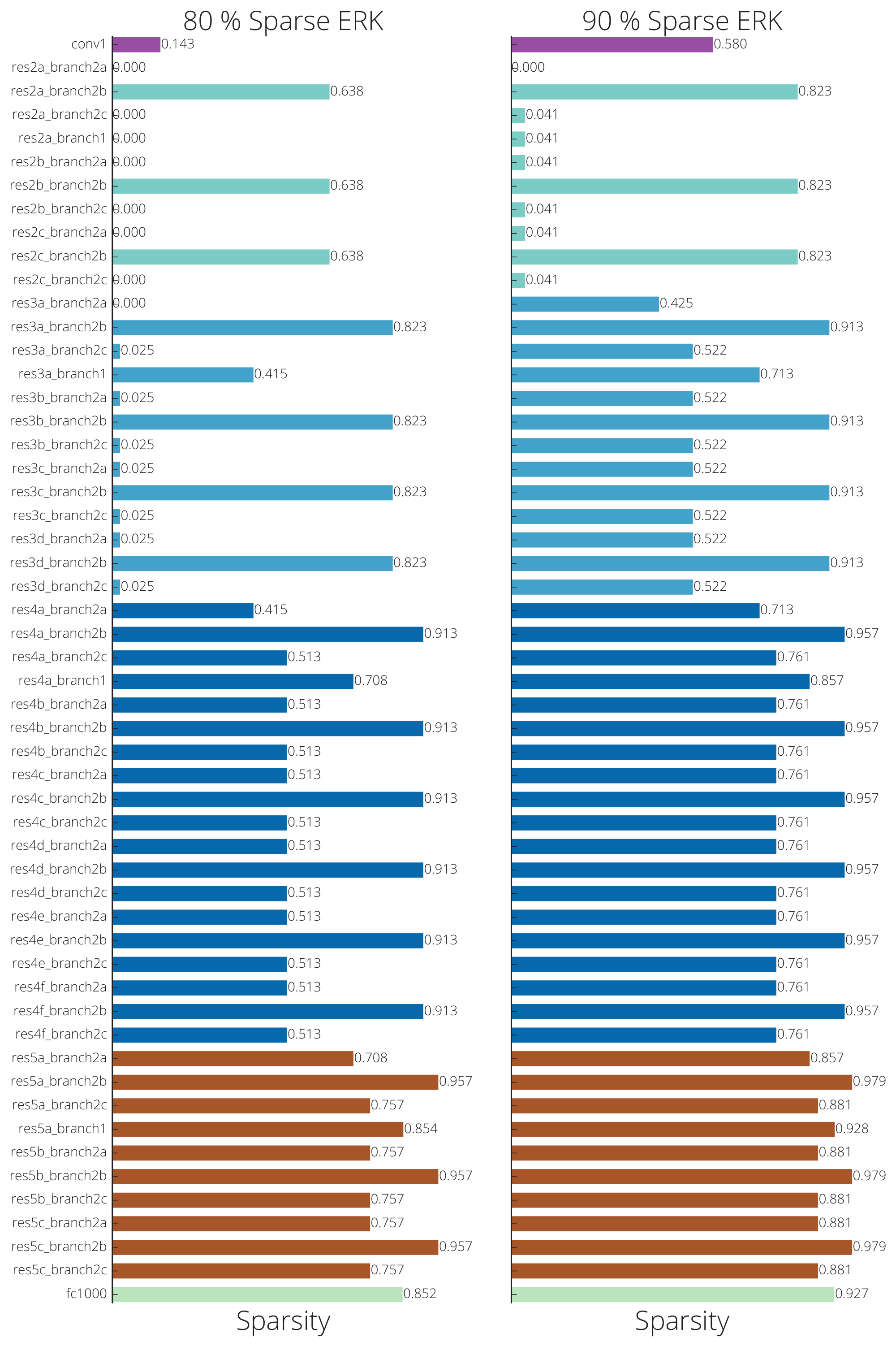
Effect of Sparsity Distribution: Figure 5-left shows how the sparsity distribution affects the final test accuracy of sparse ResNet-50s trained with RigL. Erdős-Rényi-Kernel (ERK) performs consistently better than the other two distributions. ERK automatically allocates more parameters to the layers with few parameters by decreasing their sparsities[^5]. This reallocation seems to be crucial for preserving the capacity of the network at high sparsity levels where ERK outperforms other distributions by a greater margin. Though it performs better, the ERK distribution requires approximately twice as many FLOPs compared to a uniform distribution. This highlights an interesting trade-off between accuracy and computational efficiency where better performance is obtained by increasing the number of FLOPs required to evaluate the model. This trade-off also highlights the importance of reporting non-uniform sparsities along with respective FLOPs when two networks of same sparsity (parameter count) are compared.
[^5]: see Appendix K for exact layer-wise sparsities.
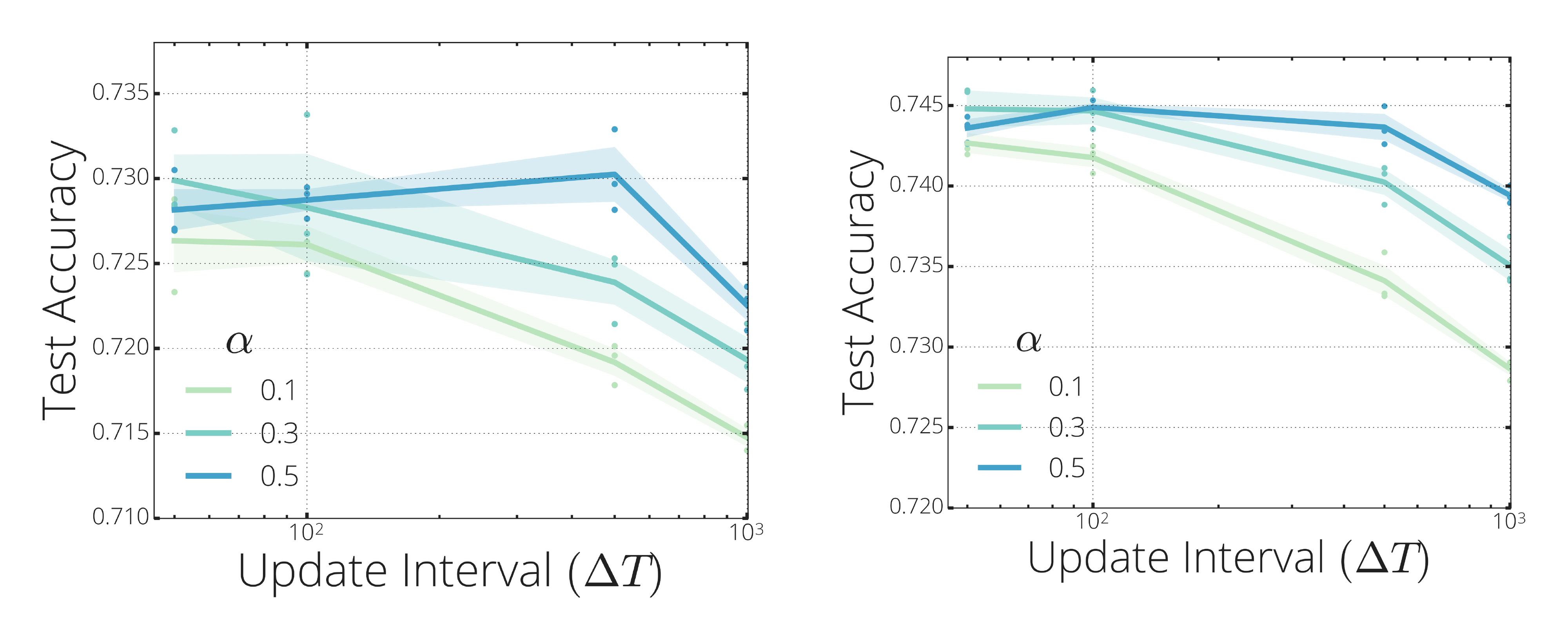
Effect of Update Schedule and Frequency: In Figure 5-right, we evaluate the performance of our method on update intervals $\Delta T\in [50, 100, 500, 1000]$ and initial drop fractions $\alpha \in [0.1, 0.3, 0.5]$. The best accuracies are obtained when the mask is updated every 100 iterations with an initial drop fraction of 0.3 or 0.5. Notably, even with infrequent update intervals (e.g. every 1000 iterations), RigL performs above 73.5%.
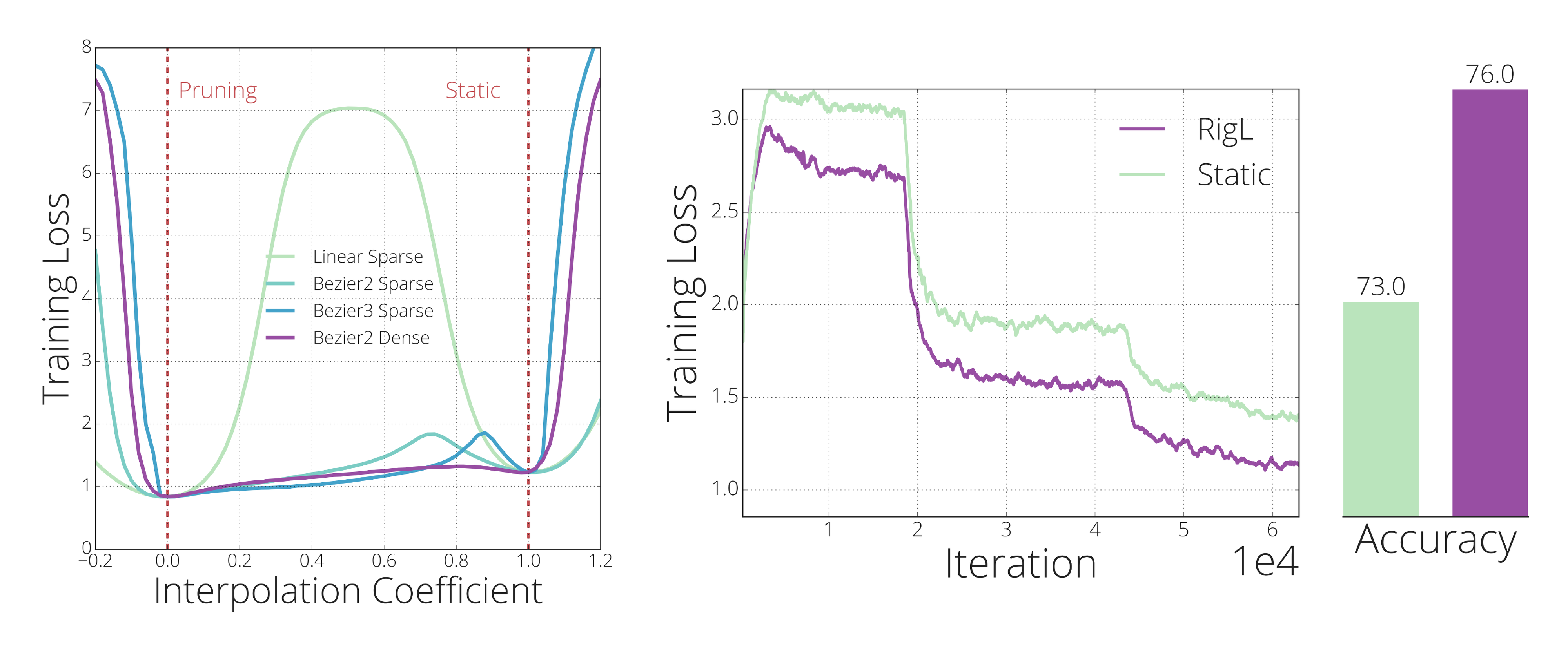
Effect of Dynamic connections: [28] and [25] observed that static sparse training converges to a solution with a higher loss than dynamic sparse training. In Figure 6-left we examine the loss landscape lying between a solution found via static sparse training and a solution found via pruning to understand whether the former lies in a basin isolated from the latter. Performing a linear interpolation between the two reveals the expected result – a high-loss barrier – demonstrating that the loss landscape is not trivially connected. However, this is only one of infinitely many paths between the two points ([43, 44]) and does not imply the nonexistence of such a path. For example [43] showed different dense solutions lie in the same basin by finding $2^{nd}$ order Bézier curves with low energy between the two solutions. Following their method, we attempt to find quadratic and cubic Bézier curves between the two sparse solutions. Surprisingly, even with a cubic curve, we fail to find a path without a high-loss barrier. These results suggest that static sparse training can get stuck at local minima that are isolated from better solutions. On the other hand, when we optimize the quadratic Bézier curve across the full dense space we find a near-monotonic path to the improved solution, suggesting that allowing new connections to grow yields greater flexibility in navigating the loss landscape.
In Figure 6-right we train RigL starting from the sub-optimal solution found by static sparse training, demonstrating that it is able to escape the local minimum, whereas re-training with static sparse training cannot. RigL first removes connections with the smallest magnitudes since removing these connections have been shown to have a minimal effect on the loss ([1, 45]). Next, it activates connections with the high gradients, since these connections are expected to decrease the loss fastest. In Appendix A we discuss the effect of RigL updates on the energy landscape.
5. Discussion & Conclusion
Section Summary: This paper introduces RigL, a new method for efficiently training sparse neural networks, which use fewer connections to save computing power while maintaining performance. RigL outperforms other similar approaches in accuracy for the same amount of computation, making it ideal for refining models before deployment, boosting large models with limited training time, and enabling the creation of massive sparse networks that were previously impossible. Although hardware support for sparsity is still developing, RigL positions itself to benefit from upcoming advancements in software and new accelerators.
In this work we introduced RigL, an algorithm for training sparse neural networks efficiently. For a given computational budget RigL achieves higher accuracies than existing dense-to-sparse and sparse-to-sparse training algorithms. RigL is useful in three different scenarios: (1) To improve the accuracy of sparse models intended for deployment; (2) To improve the accuracy of large sparse models which can only be trained for a limited number of iterations; (3) Combined with sparse primitives to enable training of extremely large sparse models which otherwise would not be possible.
The third scenario is unexplored due to the lack of hardware and software support for sparsity. Nonetheless, work continues to improve the performance of sparse networks on current hardware ([46, 47]), and new types of hardware accelerators will have better support for parameter sparsity ([48, 49, 50, 51, 52]). RigL provides the tools to take advantage of, and motivation for, such advances.
Acknowledgments
We would like to thank Eleni Triantafillou, Hugo Larochelle, Bart van Merriënboer, Fabian Pedregosa, Joan Puigcerver, Nicolas Le Roux, Karen Simonyan for giving feedback on the preprint of the paper; Namhoon Lee for helping us verifying/debugging our SNIP implementation; Chris Jones for helping discovering/solving the distributed training bug; Dyllan McCreary for helping us improve the notation; D.C. Mocanu for helping us clarify related work timeline; Varun Sundar and Rajat Vadiraj Dwaraknath for choosing our work for the ML Reproducibility Challenge 2020.
Appendix
Section Summary: The appendix explores how updating a neural network's connections by removing those with the smallest values minimizes disruption to its performance, while adding new ones with strong initial gradients helps the training process escape difficult optimization challenges, effectively smoothing the "energy landscape" for better learning. It then compares the RigL method to structured pruning techniques like SBP, L0, and VIB on a simple image recognition task using handwritten digits, demonstrating through data that RigL achieves more compact networks that use less computing power for both training and running, while maintaining similar accuracy. A figure illustrates how RigL focuses on the most important input features over time.
A. Effect of Mask Updates on the Energy Landscape
To update the connectivity of our sparse network, we first need to drop a fraction $d$ of the existing connections for each layer independently to create a budget for growing new connections. Like many prior works ([11, 12, 14, 1]), we drop parameters with the smallest magnitude. The effectiveness of this simple criteria can be explained through the first order Taylor approximation of the loss $L$ around the current set of parameters $\theta$.
$ \Delta L = L(\theta+\Delta \theta) - L(\theta) = \nabla_\theta L(\theta) \Delta \theta + R(||\Delta \theta||^2_2) $
The main goal of dropping connections is to remove parameters with minimal impact on the output of the neural network and therefore on its loss. Since removing the connection $\theta_i$ corresponds to setting it to zero, it incurs a change of $\Delta\theta=-\theta_i$ in that direction and a change of $\Delta L_i = -\nabla_{\theta_i} L(\theta)\theta_i + R(\theta_i^2)$ in the loss, where the first term is usually defined as the saliency of a connection. Saliency has been used as a criterion to remove connections ([53]), however it has been shown to produce inferior results compared to magnitude based removal, especially when used to remove multiple connections at once ([45]). In contrast, picking the lowest magnitude connections ensures a small remainder term in addition to a low saliency, limiting the damage we make when we drop connections. Additionally, we note that connections with small magnitude can only remain small if the gradient they receive during training is small, meaning that the saliency is likely small when the parameter itself is small.
After the removal of insignificant connections, we enable new connections that have the highest expected gradients. Since we initialize these new connections to zero, they are guaranteed to have high gradients in the proceeding iteration and therefore to reduce the loss quickly. Combining this observation with the fact that RigL is likely to remove low gradient directions, ) and the results in Section 4.4, suggests that RigL improves the energy landscape of the optimization by replacing flat dimensions with ones with higher gradient. This helps the optimization procedure escape saddle points.
B. Comparison with Bayesian Structured Pruning Algorithms
Structured pruning algorithms aim to remove entire neurons (or channels) instead of individual connections either at the end of, or throughout training. The final pruned network is a smaller dense network. [54] demonstrated that these smaller networks could themselves be successfully be trained from scratch. This recasts structured pruning approaches as a limited kind of architecture search, where the search space is the size of each hidden layer.
In this section we compare RigL with three different structured pruning algorithms: SBP ([22]), L0 ([18]), and VIB ([21]). We show that starting from a random sparse network, RigL finds compact networks with fewer parameters, that require fewer FLOPs for inference and require fewer resources for training. This serves as a general demonstration of the effectiveness of unstructured sparsity.
\begin{tabular}{l|cccccc}\toprule

  Method & Final & Sparsity & Training Cost & Inference Cost& Size & Error \\
  & Architecture & & (GFLOPs) & (KFLOPs) & (bytes) & \\
\midrule
SBP	& 245-160-55	& 0.000	& 13521.6 (2554.8)	& 97.1	& 195100	& 1.6 \\
L0	& 266-88-33	& 0.000	& 13521.6 (1356.4) & 53.3	& 107092	& 1.6 \\
VIB	& 97-71-33	& 0.000	& 13521.6 (523) & 19.1	& 38696	& 1.6 \\
RigL	& 408-100-69	& 0.870	& 482.0	& 12.6	& 31914	& 1.44 (1.48) \\
RigL+	& 375-62-51	& 0.886	& \textbf{206.3}	& \textbf{6.2}	& \textbf{16113}	& 1.57 (1.69) \\
\bottomrule \end{tabular}
For our setting we pick the standard LeNet 300-100 network with ReLU non-linearities trained on MNIST. In Table 2 we compare methods based on how many FLOPs they require for training and also how efficient the final architecture is. Unfortunately, none of the papers have released the code for reproducing the MLP results, so we therefore use the reported accuracies and calculate lower bounds for the the FLOPs used during training. For each method we assume that one training step takes as much as the dense 300-100 architecture and omit any additional operations each method introduces. We also consider training the pruned networks from scratch and report the training FLOPs required in parenthesis. In this setting, training FLOPs are significantly lower since the starting networks are have been significantly reduced in size. We assume that following ([54]) the final networks can be trained from scratch, but we cannot verify this for these MLP networks since it would require knowledge of which pixels were dropped from the input.
To compare, we train a sparse network starting from the original MLP architecture (RigL). At initialization, we randomly remove 99% and 89% of the connections in the first and second layer of the MLP. At the end of the training many of the neurons in the first 2 layers have no in-coming or out-going connections. We remove such neurons and use the resulting architecture to calculate the inference FLOPs and the size. We assume the sparse connectivity is stored as a bit-mask (We assume parameters are represented as floats, i.e. 4 bytes). In this setting, RigL finds smaller, more FLOP efficient networks with far less work than the Bayesian approaches.
Next, we train a sparse network starting from the architecture found by the first run (RigL+) (408-100-69) but with a new random initialization (both masks and the parameters). We reduce the sparsity of the first 2 layers to 96% and 86% respectively as the network is already much smaller. Repeating RigL training results in an even more compact architecture half the size and requiring only a third the FLOPs of the best architecture found by [21].
Examination of the open-sourced code for the methods considered here made us aware that all of them keep track of the test error during training and report the best error ever observed during training as the final error. We generally would not encourage such overfitting to the test/validation set, however to make the comparisons with these results fair we report both the lowest error observed during training and the error at the end of training (reported in parenthesis). All hyper-parameter tuning was done using only the final test error.
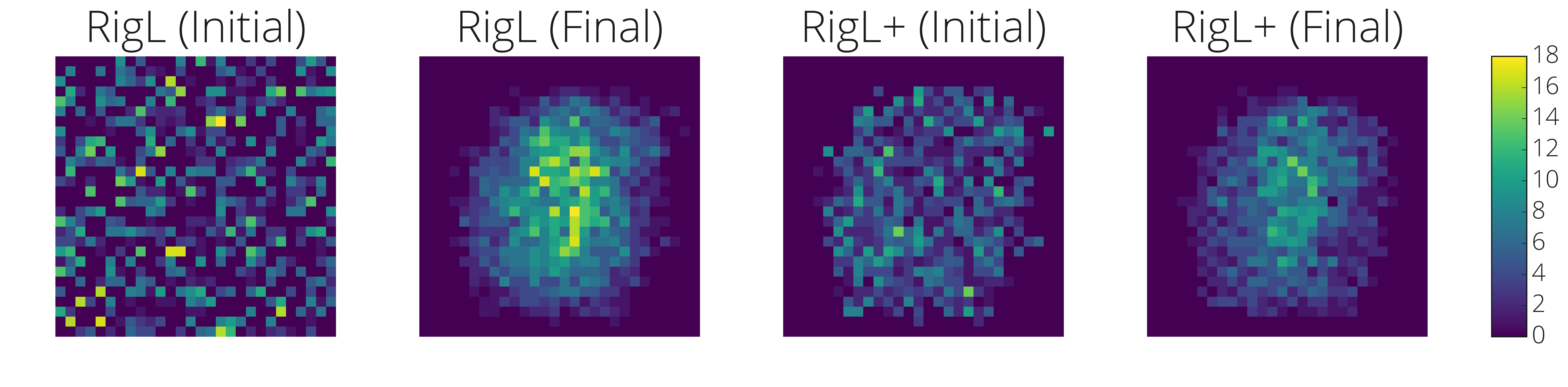
In Figure 7 we visualize how RigL chooses to connect to the input and how this evolves from the beginning to the end of training. The heatmap shows the number of outgoing connections from each input pixels at the beginning (RigL Initial) and at the end (RigL (Final)) of the training. The left two images are for the initial network and the right two images are for RigL+ training. RigL automatically discards uninformative pixels and allocates the connections towards the center highlighting the potential of RigL on model compression and feature selection.
C. Effect of Sparsity Distribution on Other Methods
In Figure 8-left we show the effect of sparsity distribution choice on 4 different sparse training methods. ERK distribution performs better than other distributions for each training method.
D. Effect of Momentum Coefficient for SNFS
In Figure 8 right we show the effect of the momentum coefficient on the performance of SNFS. Our results shows that using a coefficient of 0.99 brings the best performance. On the other hand using the most recent gradient only (coefficient of 0) performs as good as using a coefficient of 0.9. This result might be due to the large batch size we are using (4096), but it still motivates using RigL and instantaneous gradient information only when needed, instead of accumulating them.
E. (Non)-Existence of Lottery Tickets
We perform the following experiment to see whether Lottery Tickets exist in our setting. We take the sparse network found by RigL and restart training using original initialization, both with RigL and with fixed topology as in the original Lottery Ticket Hypothesis. Results in Table 3 demonstrate that training with a fixed topology is significantly worse than training with RigL and that RigL does not benefit from starting again with the final topology and the original initialization - training for twice as long instead of rewiring is more effective. In short, there are no special tickets, with RigL all tickets seems to win.
:Table 3: Effect of lottery ticket initialization on the final performance. There are no special tickets and the dynamic connectivity provided by RigL is critical for good performance.
| Initialization | Training Method | Test Accuracy | Training FLOPs |
|---|---|---|---|
| Lottery | Static | 70.82 $\pm$ 0.07 | 0.46x |
| Lottery | RigL | 73.93 $\pm$ 0.09 | 0.46x |
| Random | RigL | 74.55 $\pm$ 0.06 | 0.23x |
| Random | RigL$_{2\times}$ | 76.06 $\pm$ 0.09 | 0.46x |
F. Effect of Update Schedules on Other Dynamic Sparse Methods
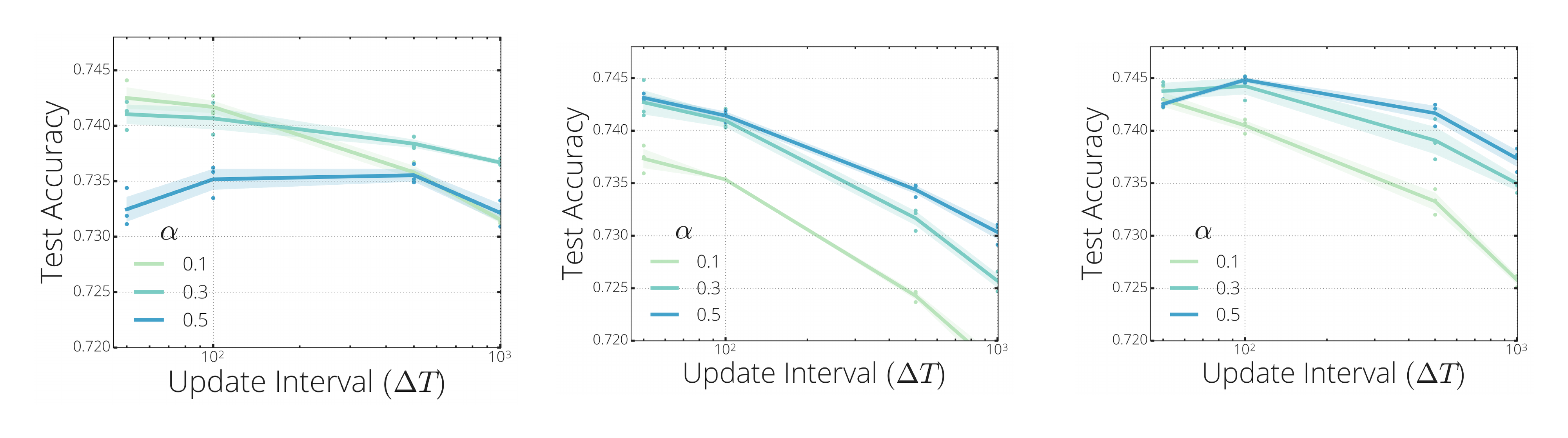
In Figure 9 we repeat the hyper-parameter sweep done for RigL in Figure 5-right, using SET and SNFS. Cosine schedule with $\Delta T=50$ and $\alpha=0.1$ seems to work best across all methods. An interesting observation is that higher drop fractions ($\alpha$) seem to work better with longer intervals $\Delta T$. For example, SET with $\Delta T=1000$ seems to work best with $\alpha=0.5$.
G. Alternative Update Schedules
In Figure 10, we share the performance of two alternative annealing functions:
- Constant: $f_{decay}(t)=\alpha$.
- Inverse Power: The fraction of weights updated decreases similarly to the schedule used in [6] for iterative pruning: $f_{decay}(t)=\alpha(1-\frac{t}{T_{end}})^k$. In our experiments we tried $k=1$ which is the linear decay and their default $k=3$.
Constant seems to perform well with low initial drop fractions like $\alpha=0.1$, but it starts to perform worse with increasing $\alpha$. Inverse Power for k=3 and k=1 (Linear) seems to perform similarly for low $\alpha$ values. However the performance drops noticeably for k=3 when we increase the update interval. As reported by [26] linear (k=1) seems to provide similar results as the cosine schedule.
H. Calculating FLOPs of models and methods
In order to calculate FLOPs needed for a single forward pass of a sparse model, we count the total number of multiplications and additions layer by layer for a given layer sparsity $s^l$. The total FLOPs is then obtained by summing up all of these multiply and adds.
Different sparsity distributions require different number of FLOPs to compute a single prediction. For example Erdős-Renyi-Kernel distributions usually cause 1x1 convolutions to be less sparse than the 3x3 bottleneck layers (see Appendix K). The number of input/output channels of 1x1 convolutional layers are greater and therefore require more FLOPs to compute the output features compared to 3x3 layers of the ResNet blocks. Thus, allocating smaller sparsities to 1x1 convolutional layers results in a higher overall FLOPs than a sparse network with uniform sparsity.
Training a neural network consists of 2 main steps:
- forward pass: Calculating the loss of the current set of parameters on a given batch of data. During this process layer activations are calculated in sequence using the previous activations and the parameters of the layer. Activation of layers are stored in memory for the backward pass.
- backward pass: Using the loss value as the initial error signal, we back-propagate the error signal while calculating the gradient of parameters. During the backward pass each layer calculates 2 quantities: the gradient of the activations of the previous layer and the gradient of its parameters. Therefore in our calculations we count backward passes as two times the computational expense of the forward pass. We omit the FLOPs needed for batch normalization and cross entropy.
Dynamic sparse training methods require some extra FLOPs to update the connectivity of the neural network. We omit FLOPs needed for dropping the lowest magnitude connections in our calculations. For a given dense architecture with FLOPs $f_D$ and a sparse version with FLOPs $f_S$, the total FLOPs required to calculate the gradient on a single sample is computed as follows:
- Static Sparse and Dense. Scales with $3f_S$ and $3f_D$ FLOPs, respectively.
- Pruning. $\mathbb{E}_t[3f_D(1-s_t)$] FLOPs where $s_t$ is the sparsity of the model at iteration $t$.
- Snip. We omit the initial dense gradient calculation since it is negligible, which means Snip scales in the same way as Static methods: $3*f_S$ FLOPs.
- SET. We omit the extra FLOPs needed for growing random connections, since this operation can be done on chip efficiently. Therefore, the total FLOPs for SET scales with $3*f_S$.
- SNFS. Forward pass and back-propagating the error signal needs $2f_S$ FLOPs. However, the dense gradient needs to be calculated at every iteration. Thus, the total number of FLOPs scales with $2f_S+f_D$.
- RigL. Iterations with no connection updates need $3f_S$ FLOPs. However, at every $\Delta T$ iteration we need to calculate the dense gradients. This results in the average FLOPs for RigL given by $\frac{(3f_S*\Delta T+2*f_S+f_D)}{(\Delta T+1)}$.
I. Hyper-parameters used in Charachter Level Language Modeling Experiments
As stated in the main text, our network consists of a shared embedding with dimensionality 128, a vocabulary size of 256, a GRU with a state size of 512, a readout from the GRU state consisting of two linear layers with width 256 and 128 respectively. We train the next step prediction task with the cross entropy loss using the Adam optimizer. We set the learning rate to $7e-4$ and L2 regularization coefficient to $5e-4$. We use a sequence length of 512 and a batch size of 32. Gradients are clipped when their magnitudes exceed 10. We set the sparsity to 75% for all models and run 200, 000 iterations. When inducing sparsity with magnitude pruning ([6]), we perform pruning between iterations 50, 000 and 150, 000 with a frequency of 1, 000. We initialize sparse networks with a uniform sparsity distribution and use a cosine update schedule with $\alpha=0.1$ and $\Delta T=100$. Unlike the previous experiments we keep updating the mask until the end of the training since we observed this performed slightly better than stopping at iteration 150, 000.
J. Additional Plots and Experiments for CIFAR-10
In Figure 11-left, we plot the final training loss of experiments presented in Section 4.3 to investigate the generalization properties of the algorithms considered. Poor performance of Static reflects itself in training loss clearly across all sparsity levels. RigL achieves similar final loss as the pruning, despite having around half percent less accuracy. Training longer with RigL decreases the final loss further and the test accuracies start matching pruning (see Figure 4-right) performance. These results show that RigL improves the optimization as promised, however generalizes slightly worse than pruning.
In Figure 11-right, we sweep mask update interval $\Delta T$ and plot the final test accuracies. We fix initial drop fraction $\alpha$ to $0.3$ and evaluate two different sparsity distributions: Uniform and ERK. Both curves follow a similar pattern as in Imagenet-2012 sweeps (see Figure 9) and best results are obtained when $\Delta T=100$.
K. Sparsity of Individual Layers for Sparse ResNet-50
Sparsity of ResNet-50 layers given by the Erdős-Rényi-Kernel sparsity distribution plotted in Figure 12.
L. Performance of Algortihms at Training 95 and 96.5% Sparse ResNet-50
In this section we share results of algorithms at training ResNet-50s with higher sparsities. Results in Table [@fig:app_highsparsity] indicate RigL achieves higher performance than the pruning algorithm even without extending training length.
\begin{tabular}{c|p{5em}|p{4em}|p{4em}||p{5em}|p{4em}|p{4em}}
  \toprule
  Method & Top-1 \newline Accuracy& FLOPs \newline (Train) & FLOPs\newline (Test) & Top-1 \newline Accuracy& FLOPs \newline (Train) & FLOPs\newline (Test) \\\toprule
  Dense & 76.8\small{$\pm$ 0.09} & 1x \small{(3.2e18)} & 1x \small{(8.2e9)} \\\hline
  & \multicolumn{3}{c ||}{S=0.95} & \multicolumn{3}{ c }{S=0.965}\\\hline \hline
  Static & 59.5+-0.11 & 0.23x & 0.08x & 55.4+-0.06 & 0.13x & 0.07x \\
  Snip & 57.8+-0.40 & 0.23x & 0.08x & 52.0+-0.20 & 0.13x & 0.07x \\
  SET & 64.4+-0.77 & 0.23x & 0.08x & 60.8+-0.45 & 0.13x & 0.07x \\
  RigL & 67.5+-0.10 & 0.23x & 0.08x & 65.0+-0.28 & 0.13x & 0.07x \\
  RigL$_{5\times}$ & 73.1+-0.12 & 1.14x & 0.08x & 71.1+-0.20 & 0.66x & 0.07x \\\hline
  Static (ERK) & 72.1\small{$\pm$ 0.04} & 0.42x & 0.42x & 67.7\small{$\pm$ 0.12} & 0.24x & 0.24x \\
  RigL (ERK) & 69.7+-0.17 & 0.42x & 0.12x & 67.2+-0.06 & 0.25x & 0.11x \\
RigL$_{5\times}$ (ERK) & 74.5+-0.09 & 2.09x & 0.12x & 72.7+-0.02 & 1.23x & 0.11x \\\hline \hline
  SNFS (ERK) & 70.0+-0.04 & 0.61x & 0.12x & 67.1+-0.72 & 0.50x & 0.11x \\
  Pruning* (Gale) & 70.6 & 0.56x & 0.08x & n/a & 0.51x & 0.07x \\
  Pruning$_{1.5\times}$ (Gale) & 72.7 & 0.84x & 0.08x & 69.26 & 0.76x & 0.07x
  \\
  \bottomrule
  \end{tabular}
M. Bugs Discovered During Experiments
Our initial implementations contained some subtle bugs, which while not affecting the general conclusion that RigL is more effective than other techniques, did result in lower accuracy for all sparse training techniques. We detail these issues here with the hope that others may learn from our mistakes.
- Random operations on multiple replicas. We use data parallelism to split a mini-batch among multiple replicas. Each replica independently calculates the gradients using a different sub-mini-batch of data. The gradients are aggregated using an $\textsc{all-reduce}$ operation before the optimizer update. Our implementation of SET, SNFS and RigL depended on each replica independently choosing to drop and grow the same connections. However, due to the nature of random operations in Tensorflow, this did not happen. Instead, different replicas diverged after the first drop/grow step. This was most pronounced in SET where each replica chose at random and much less so for SNFS and RigL where randomness is only needed to break ties. If left unchecked this might be expected to be catastrophic, but due to the behavior of Estimators and/or TF-replicator, the values on the first replica are broadcast to the others periodically (every approximately 1000 steps in our case).
We fixed this bug by using stateless random operations. As a result the performance of SET improved slightly (0.1-0.3 % higher on Figure 2-left). 2. Synchronization between replicas. RigL and SNFS depend on calculating dense gradients with respect to the masked parameters. However, as explained above, in the multiple replica setting these gradients need to be aggregated. Normally this aggregation is automatically done by the optimizer, but in our case, this does not happen (only the gradients with respect to the unmasked parameters are aggregated automatically). This bug affected SNFS and RigL, but not SET since SET does not rely on the gradients to grow connections. Again, the synchronization of the parameters from the first replica every approximately 1000 steps masked this bug.
We fixed this bug by explicitly calling $\textsc{all-reduce}$ on the gradients with respect to the masked parameters. With this fix, the performance of RigL and SNFS improved significantly, particularly for default training lengths (around 0.5-1% improvement). 3. SNIP Experiments. Our first implementation of SNIP used the gradient magnitudes to decide which connections to keep causing its performance to be worse than static. Upon our discussions with the authors of SNIP, we realized that the correct metric is the saliency (gradient times parameter magnitude). With this correction SNIP performance improved dramatically to better than random (Static) even at Resnet-50/ImageNet scale. It is surprising that picking connections with the highest gradient magnitudes can be so detrimental to training (it resulted in much worse than random performance).
N. Changes Since Publishing
- The ordering of SET and NeST updated after learning SET was published earlier
- $\mathbb{I}{drop}$ notation is replaced by $\mathbb{I}{active}$ to make it more clear that the indices captured by the notation are the connections kept.
- Typo at pruning flops calculation is fixed (kudos to Varun Sundar for reporting).
- Zero initialization at growth is emphasized and together with some other choices attempted.
References
[1] Han, S., Pool, J., Tran, J., and Dally, W. Learning both weights and connections for efficient neural network. In Advances in Neural Information Processing Systems, 2015.
[2] Srinivas, S., Subramanya, A., and Babu, R. V. Training sparse neural networks. In 2017 IEEE Conference on Computer Vision and Pattern Recognition Workshops (CVPRW), 2017.
[3] Kalchbrenner, N., Elsen, E., Simonyan, K., Noury, S., Casagrande, N., Lockhart, E., Stimberg, F., Oord, A., Dieleman, S., and Kavukcuoglu, K. Efficient neural audio synthesis. In International Conference on Machine Learning, 2018.
[4] Park, J., Li, S. R., Wen, W., Li, H., Chen, Y., and Dubey, P. Holistic SparseCNN: Forging the trident of accuracy, speed, and size. ArXiv, 2016. URL http://arxiv.org/abs/1608.01409.
[5] Elsen, E., Dukhan, M., Gale, T., and Simonyan, K. Fast sparse convnets. ArXiv, 2019. URL https://arxiv.org/abs/1911.09723.
[6] Zhu, M. and Gupta, S. To prune, or not to prune: Exploring the efficacy of pruning for model compression. In International Conference on Learning Representations Workshop, 2018. URL https://arxiv.org/abs/1710.01878.
[7] Guo, Y., Yao, A., and Chen, Y. Dynamic network surgery for efficient DNNs. ArXiv, 2016. URL http://arxiv.org/abs/1608.04493.
[8] Molchanov, D., Ashukha, A., and Vetrov, D. P. Variational Dropout Sparsifies Deep Neural Networks. In International Conference on Machine Learning, pp.\ 2498–2507, 2017.
[9] Gale, T., Elsen, E., and Hooker, S. The state of sparsity in deep neural networks. ArXiv, 2019. URL http://arxiv.org/abs/1902.09574.
[10] Frankle, J. and Carbin, M. The lottery ticket hypothesis: Finding sparse, trainable neural networks. In International Conference on Learning Representations, 2019. URL https://openreview.net/forum?id=rJl-b3RcF7.
[11] Thimm, G. and Fiesler, E. Evaluating pruning methods. In Proceedings of the International Symposium on Artificial Neural Networks, 1995.
[12] Ström, N. Sparse Connection and Pruning in Large Dynamic Artificial Neural Networks. In EUROSPEECH, 1997.
[13] Han, S., Mao, H., and Dally, W. J. Deep compression: Compressing deep neural network with pruning, trained quantization and huffman coding. In International Conference on Learning Representations, 2016b. URL http://arxiv.org/abs/1510.00149.
[14] Narang, S., Diamos, G., Sengupta, S., and Elsen, E. Exploring sparsity in recurrent neural networks. In International Conference on Learning Representations, 2017. URL https://openreview.net/forum?id=BylSPv9gx.
[15] Mozer, M. C. and Smolensky, P. Skeletonization: A technique for trimming the fat from a network via relevance assessment. In Advances in Neural Information Processing Systems, 1989.
[16] LeCun, Y., Denker, J. S., and Solla, S. A. Optimal Brain Damage. In Advances in Neural Information Processing Systems, 1990.
[17] Hassibi, B. and Stork, D. Second order derivatives for network pruning: Optimal Brain Surgeon. In Advances in Neural Information Processing Systems, 1993.
[18] Christos Louizos, Max Welling, D. P. K. Learning sparse neural networks through $l_0$ regularization. In International Conference on Learning Representations, 2018.
[19] Wortsman, M., Farhadi, A., and Rastegari, M. Discovering neural wirings. ArXiv, 2019. URL http://arxiv.org/abs/1906.00586.
[20] Tartaglione, E., Lepsøy, S., Fiandrotti, A., and Francini, G. Learning sparse neural networks via sensitivity-driven regularization. In Advances in Neural Information Processing Systems, 2018. URL http://dl.acm.org/citation.cfm?id=3327144.3327303.
[21] Dai, B., Zhu, C., Guo, B., and Wipf, D. Compressing neural networks using the variational information bottleneck. In International Conference on Machine Learning, 2018.
[22] Neklyudov, K., Molchanov, D., Ashukha, A., and Vetrov, D. Structured bayesian pruning via log-normal multiplicative noise. In Advances in Neural Information Processing Systems, 2017.
[23] Mocanu, D. C., Mocanu, E., Stone, P., Nguyen, P. H., Gibescu, M., and Liotta, A. Scalable training of artificial neural networks with adaptive sparse connectivity inspired by network science. Nature Communications, 2018. URL http://www.nature.com/articles/s41467-018-04316-3.
[24] Bellec, G., Kappel, D., Maass, W., and Legenstein, R. A. Deep rewiring: Training very sparse deep networks. In International Conference on Learning Representations, 2018.
[25] Mostafa, H. and Wang, X. Parameter efficient training of deep convolutional neural networks by dynamic sparse reparameterization. In International Conference on Machine Learning, 2019. URL http://proceedings.mlr.press/v97/mostafa19a.html.
[26] Dettmers, T. and Zettlemoyer, L. Sparse networks from scratch: Faster training without losing performance. ArXiv, 2019. URL http://arxiv.org/abs/1907.04840.
[27] Lee, N., Ajanthan, T., and Torr, P. H. S. SNIP: Single-shot Network Pruning based on Connection Sensitivity. In International Conference on Learning Representations, 2019.
[28] Frankle, J., Dziugaite, G. K., Roy, D. M., and Carbin, M. The lottery ticket hypothesis at scale. ArXiv, 2019. URL http://arxiv.org/abs/1903.01611.
[29] He, K., Zhang, X., Ren, S., and Sun, J. Delving deep into rectifiers: Surpassing human-level performance on imagenet classification. In Proceedings of the 2015 IEEE International Conference on Computer Vision (ICCV), 2015.
[30] Zhou, H., Lan, J., Liu, R., and Yosinski, J. Deconstructing lottery tickets: Zeros, signs, and the supermask. ArXiv, 2019. URL http://arxiv.org/abs/1905.01067.
[31] Russakovsky, O., Deng, J., Su, H., Krause, J., Satheesh, S., Ma, S., Huang, Z., Karpathy, A., Khosla, A., Bernstein, M., Berg, A. C., and Fei-Fei, L. Imagenet large scale visual recognition challenge. International Journal of Computer Vision (IJCV), 2015.
[32] Krizhevsky, A. Learning multiple layers of features from tiny images. In University of Toronto, 2009. URL https://www.cs.toronto.edu/~kriz/learning-features-2009-TR.pdf.
[33] Merity, S., Xiong, C., Bradbury, J., and Socher, R. Pointer sentinel mixture models. ArXiv, 2016. URL http://arxiv.org/abs/1609.07843.
[34] Abadi, M., Agarwal, A., Barham, P., Brevdo, E., Chen, Z., Citro, C., Corrado, G. S., Davis, A., Dean, J., Devin, M., Ghemawat, S., Goodfellow, I., Harp, A., Irving, G., Isard, M., Jia, Y., Jozefowicz, R., Kaiser, L., Kudlur, M., Levenberg, J., Mané, D., Monga, R., Moore, S., Murray, D., Olah, C., Schuster, M., Shlens, J., Steiner, B., Sutskever, I., Talwar, K., Tucker, P., Vanhoucke, V., Vasudevan, V., Viégas, F., Vinyals, O., Warden, P., Wattenberg, M., Wicke, M., Yu, Y., and Zheng, X. TensorFlow: Large-scale machine learning on heterogeneous systems, 2015. URL http://tensorflow.org/.
[35] Sundar, V. and Dwaraknath, R. V. [reproducibility report] rigging the lottery: Making all tickets winners. arXiv, 2021.
[36] Szegedy, C., Vanhoucke, V., Ioffe, S., Shlens, J., and Wojna, Z. Rethinking the inception architecture for computer vision. In Proceedings of IEEE Conference on Computer Vision and Pattern Recognition,, 2016. URL http://arxiv.org/abs/1512.00567.
[37] Kusupati, A., Ramanujan, V., Somani, R., Wortsman, M., Jain, P., Kakade, S., and Farhadi, A. Soft threshold weight reparameterization for learnable sparsity. In International Conference on Machine Learning, 2020.
[38] Evci, U., Pedregosa, F., Gomez, A. N., and Elsen, E. The difficulty of training sparse neural networks. ArXiv, 2019. URL http://arxiv.org/abs/1906.10732.
[39] Howard, A. G., Zhu, M., Chen, B., Kalenichenko, D., Wang, W., Weyand, T., Andreetto, M., and Adam, H. Mobilenets: Efficient convolutional neural networks for mobile vision applications. ArXiv, 2017. URL http://arxiv.org/abs/1704.04861.
[40] Sandler, M., Howard, A., Zhu, M., Zhmoginov, A., and Chen, L. Mobilenetv2: Inverted residuals and linear bottlenecks. In 2018 IEEE/CVF Conference on Computer Vision and Pattern Recognition, 2018.
[41] Cho, K., van Merrienboer, B., Gulcehre, C., Bougares, F., Schwenk, H., and Bengio, Y. Learning phrase representations using rnn encoder-decoder for statistical machine translation. In Conference on Empirical Methods in Natural Language Processing (EMNLP 2014), 2014.
[42] Zagoruyko, S. and Komodakis, N. Wide residual networks. In British Machine Vision Conference, 2016. URL http://www.bmva.org/bmvc/2016/papers/paper087/index.html.
[43] Garipov, T., Izmailov, P., Podoprikhin, D., Vetrov, D. P., and Wilson, A. G. Loss surfaces, mode connectivity, and fast ensembling of dnns. In Advances in Neural Information Processing Systems, 2018.
[44] Draxler, F., Veschgini, K., Salmhofer, M., and Hamprecht, F. A. Essentially no barriers in neural network energy landscape. In International Conference on Machine Learning, 2018. URL http://proceedings.mlr.press/v80/draxler18a/draxler18a.pdf.
[45] Evci, U. Detecting dead weights and units in neural networks. ArXiv, 2018. URL http://arxiv.org/abs/1806.06068.
[46] Hong, C., Sukumaran-Rajam, A., Nisa, I., Singh, K., and Sadayappan, P. Adaptive sparse tiling for sparse matrix multiplication. In Proceedings of the 24th Symposium on Principles and Practice of Parallel Programming, 2019. URL http://doi.acm.org/10.1145/3293883.3295712.
[47] Merrill, D. and Garland, M. Merge-based sparse matrix-vector multiplication (spmv) using the csr storage format. In Proceedings of the 21st ACM SIGPLAN Symposium on Principles and Practice of Parallel Programming, 2016. URL http://doi.acm.org/10.1145/2851141.2851190.
[48] Wang, P., Ji, Y., Hong, C., Lyu, Y., Wang, D., and Xie, Y. Snrram: An efficient sparse neural network computation architecture based on resistive random-access memory. In Proceedings of the 55th Annual Design Automation Conference, 2018. URL http://doi.acm.org/10.1145/3195970.3196116.
[49] Mike Ashby, Christiaan Baaij, P. B. M. B. O. B. A. C. C. C. L. C. S. D. N. v. D. J. F. G. H. B. H. D. P. J. S. S. S. Exploiting unstructured sparsity on next-generation datacenter hardware. 2019. URL https://myrtle.ai/wp-content/uploads/2019/06/IEEEformatMyrtle.ai_.21.06.19_b.pdf.
[50] Liu, C., Bellec, G., Vogginger, B., Kappel, D., Partzsch, J., Neumaerker, F., Höppner, S., Maass, W., Furber, S. B., Legenstein, R. A., and Mayr, C. Memory-efficient deep learning on a spinnaker 2 prototype. In Front. Neurosci., 2018.
[51] Han, S., Liu, X., Mao, H., Pu, J., Pedram, A., Horowitz, M. A., and Dally, W. J. EIE: Efficient Inference Engine on compressed deep neural network. In Proceedings of the 43rd International Symposium on Computer Architecture, 2016a.
[52] Chen, Y., Yang, T., Emer, J., and Sze, V. Eyeriss v2: A flexible accelerator for emerging deep neural networks on mobile devices. IEEE Journal on Emerging and Selected Topics in Circuits and Systems, 9(2):292–308, June 2019. doi:10.1109/JETCAS.2019.2910232.
[53] Molchanov, P., Tyree, S., Karras, T., Aila, T., and Kautz, J. Pruning Convolutional Neural Networks for Resource Efficient Transfer Learning. ArXiv, 2016. URL https://arxiv.org/abs/1611.06440.
[54] Liu, Z., Sun, M., Zhou, T., Huang, G., and Darrell, T. Rethinking the value of network pruning. In International Conference on Learning Representations, 2019.