Scaling Laws for Agent Harnesses via Effective Feedback Compute

Xuanliang Zhang Dingzirui Wang Keyan Xu Qingfu Zhu Wanxiang Che$^{*}$ Harbin Institute of Technology xuanliangzhang, dzrwang, kyxu, qfzhu, [email protected]

$^{*}$ Corresponding author.

Abstract

Agent harnesses increasingly determine the performance of language-model systems by deciding how models call tools, receive feedback, verify intermediate states, store memory, and revise solutions. Yet current test-time scaling analyses often parameterize this process by raw expenditure—tokens, tool calls, operations, wall time, or cost—which does not distinguish useful feedback from redundant or unstable interaction. We introduce Effective Feedback Compute (EFC), a trace-level scaling coordinate that credits feedback only when it is informative, valid, non-redundant, and retained for subsequent decisions, and we normalize it by task demand when comparing tasks with different feedback requirements. Across synthetic controllable tasks, executable code tasks, real benchmark traces, held-out splits, and a prospective validation batch, EFC-based coordinates consistently predict failure rates better than raw-compute baselines and a strong multivariate SAS baseline. In controlled scaling, raw tokens and tool calls explain limited variation ($R^2=0.33$ and $0.42$), SAS reaches $0.88$, while Oracle-EFC and Estimated-EFC reach $0.94$ and Oracle-EFC/ $D_{\mathrm{task}}$ reaches $0.99$. Matched-budget interventions show that improving feedback quality raises success from $0.27$ to $0.90$ while raw cost and tool calls are fixed. On mixed real traces, NRS-EFC/ $D_{\mathrm{task}}$ reaches $R^2=0.92$ while raw compute has near-zero or negative fit, and it remains the best predictor in a prospective holdout ($R^2=0.85$). These results suggest that harness scaling is governed less by how much computation is spent than by how efficiently raw budget is converted into durable, task-sufficient feedback.

Executive Summary: The document addresses a practical challenge in building reliable AI agent systems: although "agent harnesses" (the software layers that let language models call tools, receive observations, verify results, retain memory, and iterate) now drive most performance gains, there is no reliable way to predict when spending more inference-time resources will actually improve outcomes. Raw measures of effort such as tokens used, tool calls made, or wall-clock time explain little of the observed variation in success, creating uncertainty for anyone deciding how to allocate compute, design harnesses, or set budgets.

The work set out to identify a single, practical scaling coordinate that predicts agent-harness failure rates more accurately than raw expenditure or existing multivariate baselines, and to explain why the coordinate works.

Researchers ran controlled experiments on synthetic tasks with known solutions, executable code-repair tasks, and real benchmark traces from HumanEval, Terminal-Bench, and SWE-bench. They compared raw-compute measures, a strong existing system-level baseline (SAS), and several variants of a new quantity called Effective Feedback Compute (EFC). EFC awards credit to a feedback event only when it is informative, valid, non-redundant, and actually retained for later decisions; variants normalize EFC by estimated task demand or filter for stable, non-repeated observations. The analyses included matched-budget interventions that held raw cost fixed while varying feedback quality, trace-time estimation of EFC without oracle state, module ablations, cross-task prediction, held-out splits, and a prospective validation batch collected after the evaluation protocol was fixed.

The central findings are straightforward. First, raw tokens, tool calls, operations, and cost explain only modest variation in failure rates (R² typically 0.33–0.42), while EFC-based coordinates reach R² of 0.94–0.99 and far lower error; normalizing by task demand produces the strongest results. Second, success can be raised from 0.27 to 0.90 at identical raw budgets simply by improving feedback quality. Third, on mixed real traces the best EFC variant reaches R² of 0.92 and remains the strongest predictor (R² 0.85) on the fully prospective hold-out; raw measures show near-zero or negative fit. Fourth, two mechanisms explain the gains: harness efficiency (how much useful feedback a harness extracts per unit of raw spend) varies sharply across designs and tasks, while task-demand normalization removes residual scale differences when comparing dissimilar problems.

These results indicate that harness performance is governed by how efficiently raw computation is turned into durable, task-relevant feedback rather than by the amount of computation spent. Consequently, decisions about model choice, harness architecture, or budget allocation should focus on measurable feedback quality and sufficiency relative to task requirements, not on raw spend or simple interaction counts. Organizations that continue to optimize for tokens or tool calls risk large wasted expenditure; those that track EFC can achieve comparable or better reliability at lower cost.

The authors recommend three concrete next steps: adopt EFC (or its Estimated or NRS variants) as the primary scaling coordinate for harness evaluation and adaptive budget allocation; calibrate task-demand factors on each new task mixture before comparing runs; and use EFC as an explicit objective when designing or optimizing harness components such as routing, verification, and memory. They note that the current evidence is strongest on verifiable tasks with clear feedback signals and that further work is needed to extend reliable EFC estimation to open-ended environments.

The main limitations are the reliance on tasks that admit automatic verification, the need for task-specific calibration of the demand normalizer when task mixtures change, and the fact that all reported numbers come from a modest set of models and harness families. Within these boundaries the prospective validation and consistent outperformance across controlled, semi-realistic, and real traces give high confidence that EFC is a materially better coordinate than the raw alternatives examined.

1. Introduction

Section Summary: As language models shift from simple text prediction to interactive problem-solving, their success depends heavily on the surrounding agent harness that manages tool calls, feedback loops, memory, error repair, and stopping decisions. Raw spending on tokens or tool calls often fails to predict gains because much of the resulting information is unhelpful, redundant, or ignored, creating a need for a better scaling coordinate. The paper therefore proposes Effective Feedback Compute (EFC) to quantify only the useful, retained feedback an agent actually produces, along with related measures of harness efficiency and task demand, and shows that these quantities explain performance improvements far more reliably than raw compute across controlled and realistic tasks.

As language models move from single-turn prediction to interactive problem solving, performance increasingly depends on the agent harness around the base model. A harness determines how the model calls tools, receives feedback, stores memory, verifies intermediate results, repairs errors, and decides when to stop. This makes harness design a central form of test-time scaling: instead of only making the base model larger, one can spend additional inference-time computation to obtain and use evidence from the environment. However, unlike pretraining, where model size, data, and compute provide well-studied scaling coordinates, agent harnesses lack a clear scalar that predicts when additional test-time computation will improve performance. Raw expenditure alone is insufficient, because two trajectories with the same number of tokens or tool calls can differ sharply in whether their observations are useful, valid, non-redundant, and retained for later decisions. This gap motivates our central question: what quantity should serve as the scaling coordinate for closed-loop agent harness performance?

We propose Effective Feedback Compute (EFC) as such a coordinate. EFC measures the amount of useful closed-loop feedback produced by a trajectory. A feedback event receives credit only when it is informative, valid, non-redundant, and retained for later decisions. This definition separates raw spending from feedback that can actually change the agent's future behavior. We also introduce two derived quantities. Harness efficiency $\eta=\mathrm{EFC}/C_{\mathrm{raw}}$ measures raw-to-EFC conversion, namely how much effective feedback a harness extracts per unit of raw budget. Task-demand normalization, $\mathrm{EFC}/D_{\mathrm{task}}$, measures whether the extracted feedback is sufficient relative to the task's feedback requirement. For real execution traces, where repeated and unstable observations are common, we use non-redundant stable EFC (NRS-EFC) to emphasize retained feedback rather than transient interaction.

We test whether EFC explains harness scaling better than raw compute across synthetic controllable tasks, semi-realistic executable code tasks, and real benchmarks. We compare EFC coordinates against raw tokens, tool calls, wall time, operations, raw cost, and SAS, a strong multivariate agent-system scaling baseline ([1]). In controlled scaling experiments, raw tokens and tool calls explain only limited variation ($R^2=0.33$ and $0.42$), while SAS reaches $0.88$. Oracle-EFC and Estimated-EFC both improve to $0.94$, and Oracle-EFC/ $D_{\mathrm{task}}$ reaches $0.99$ with MAE $0.02$. In matched-budget interventions, changing feedback quality increases success from $0.27$ to $0.90$ while raw cost and tool calls remain matched. In trace-time estimation experiments, Estimated-EFC/ $D_{\mathrm{task}}$ reaches $R^2=0.93$, showing that the coordinate can be recovered before the final outcome is observed.

We further decompose why the coordinate works. Harness design controls raw-to-EFC conversion through routing, verification, memory, and observation quality. Across module ablations, harness efficiency explains success variation with $R^2=0.97$, while raw cost explains almost none. Task demand controls the scale on which feedback becomes sufficient. In cross-family prediction, Oracle-EFC improves over raw compute, but Oracle-EFC/ $D_{\mathrm{task}}$ raises the fit to $R^2=0.96$. On mixed real traces, raw-compute baselines have near-zero or negative fit, while NRS-EFC reaches $R^2=0.89$ and NRS-EFC/ $D_{\mathrm{task}}$ reaches $0.92$. The corresponding efficiency analysis shows that $\eta$ is slice-dependent rather than globally fixed: later harnesses dominate HumanEval-style code execution, all harnesses remain low-efficiency on Terminal tasks, and SWE tasks favor earlier or mid-stage variants. Finally, in a prospective holdout evaluated under a prespecified metric and calibration protocol, NRS-EFC/ $D_{\mathrm{task}}$ remains the best predictor with held-out $R^2=0.85$.

Our contributions are threefold. (i) We formalize EFC as a trace-level measure of useful feedback for closed-loop agent harnesses, together with Estimated-EFC and NRS-EFC for settings without oracle state access. (ii) We show that EFC and task-demand-normalized EFC outperform raw-compute baselines and SAS as scaling coordinates across controlled, executable, real, held-out, and prospective evaluations. (iii) We decompose harness scaling into harness efficiency and task demand, showing that successful harnesses must both convert raw budget into effective feedback and measure that feedback against the right task scale.

2. Problem Formulation and Experimental Setup

Section Summary: The section investigates whether agent harness performance reduces to a single scaling variable by modeling harnesses as closed-loop systems that plan, act, observe feedback, and update internal states, with success defined as the fraction of tasks solved under varying budgets. Experiments span three layers of tasks—from fully synthetic ones with known answers to realistic code and software-engineering benchmarks—while testing seven harness families, several base models, and repeated runs to isolate raw resource use from actually useful feedback. Performance predictors based on an estimated feedback coefficient are then compared against simple counts of tokens, tool calls, or operations and against a multivariate system-level baseline.

We study whether the performance of agent harnesses can be explained by a single scaling variable. Unlike standard inference-time scaling, where the main resource is often a token budget or a number of samples, agent harnesses execute closed-loop computations: they plan, act, observe external feedback, and update their internal state. Our goal is to separate raw expenditure from feedback that is actually useful for solving the task.

2.1 Agent Harnesses as Closed-Loop Computation

Let $\mathcal{T}$ denote a task distribution. A task instance $x \sim \mathcal{T}$ specifies an initial state, an instruction, an environment interface, and an evaluation function. An agent harness $h \in \mathcal{H}$, paired with a base model $m$, produces a trajectory

$ \tau = {(s_t, a_t, o_t, u_t)}_{t=1}^{T}, $

where $s_t$ is the agent state before step $t$, $a_t$ is a model action or tool call, $o_t$ is the resulting observation, and $u_t$ is the harness update to the agent state, memory, plan, or candidate solution. The horizon $T$ is determined by the harness stopping rule or by a budget limit. Each run returns a final answer $\hat{y}$, which is evaluated by a task-specific checker $g_x(\hat{y}) \in {0, 1}$. We define

$ S(x, h, m, b) = \mathbb{E}[g_x(\hat{y})], \qquad E(x, h, m, b) = 1 - S(x, h, m, b), $

where $b$ denotes the raw budget configuration. We report both instance-level success and aggregated failure rate over task families, harnesses, models, and budget levels.

2.2 Task Layers

We evaluate harness scaling on three task layers that progressively reduce oracle access while preserving automatic evaluation.

Synthetic controllable tasks. We use procedurally generated Needle Lookup, State Tracking, and Rule Filter tasks with hidden state and deterministic answers. This layer supports direct measurement of Oracle-EFC and controlled variation in $D_{\mathrm{task}}$.
Semi-realistic executable tasks. We use HumanEval-style code tasks and small executable repair or analysis tasks with unit-test or reference-check feedback. This layer tests whether Estimated-EFC remains predictive when traces contain realistic model errors.
Real benchmark subsets. We use verifiable HumanEval [2], Terminal-Bench 2.0 [3], and SWE-bench Verified [4]. This layer tests transfer to realistic agent trajectories.

Unless otherwise stated, results are aggregated at the run level and reported with task-family stratification. Additional dataset details and filtering rules are provided in Appendix A.

Unless otherwise stated, run-level quantities are first computed per run and then aggregated into the evaluation groups used by each experiment.

2.3 Harness Families

We compare seven harness families, denoted H0–H6, that differ in how they convert raw budget into useful feedback.

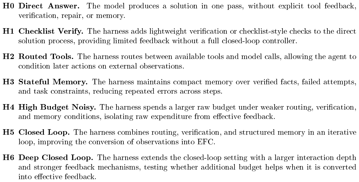
The exact prompts, tool interfaces, stopping rules, and memory formats are reported in Appendix C.

2.4 Models, Budgets, and Repeated Runs

We evaluate each task–harness configuration with multiple base models, including DeepSeek-V4-Flash, gpt-5.4-nano, and Claude-Haiku-4.5. Unless stated otherwise, all reported numbers in the paper are first aggregated over repeated runs within each model and then averaged across models.

For each task and harness, we sweep raw-budget levels that constrain model generation, tool use, harness operations, and runtime. Repeated runs estimate run-level success and failure rates under stochastic decoding. This design separates three factors that are often conflated: base-model capability, raw budget, and the amount of useful feedback captured by EFC.

2.5 Scalar Predictors and Baselines

We compare EFC-based predictors against standard raw-compute baselines and a strong system-level baseline. For each run, we record the following trace-observable quantities:

Raw Tokens: total input and output tokens consumed by the model.
Tool calls: number of external tool invocations.
Wall time: elapsed runtime of the harness.
Operations: total number of model, tool, verification, and memory-update operations.
Raw cost: a normalized cost combining token usage, tool calls, operations, and runtime.

We also include SAS [1], a prior agent-systems scaling baseline that uses a fixed-effect equation over system-level quantities. In our implementation, SAS is fit from trace-observable proxies including model strength, tool count, agent count, overhead, coordination efficiency, redundancy, error amplification, effective actions, and a single-agent baseline. SAS therefore serves as a strong multivariate baseline for system-level scaling models.

3. Effective Feedback Compute

Section Summary: Effective Feedback Compute (EFC) is a scalar that quantifies how much useful, closed-loop feedback an agent produces during a task by scoring individual events on whether they supply new task-relevant information, rest on reliable evidence, address the active subgoal, and get retained in memory. Each qualifying event earns a contribution that is the product of four [0,1] factors, and these are summed across the whole trajectory to produce a run-level total; when ground-truth state is unavailable the same quantity is estimated from observable trace features such as checker firings or plan updates. The resulting score is further normalized by a task-demand factor that accounts for search difficulty and verification noise, allowing EFC to serve as a predictor of performance scaling that is more informative than raw compute alone.

We define Effective Feedback Compute (EFC) as a scalar measure of useful closed-loop feedback produced by an agent harness. A feedback event receives credit when it reveals task-relevant information, is grounded in reliable evidence, addresses the active subgoal, and is retained for later decisions.

3.1 Feedback Events

Given a trajectory

$ \tau = {(s_i, a_i, o_i, u_i)}_{i=1}^{T},\tag{1} $

where $s_i$ is the current state, $a_i$ is an action, $o_i$ is an observation, and $u_i$ is a state or memory update, we extract a sequence of feedback events $\mathcal{E}(\tau)={e_t}{t=1}^{T{\mathrm{fb}}}$. Each event $e_t$ is a closed-loop segment in which the agent acts under a current state or subgoal, receives feedback, and updates its subsequent behavior. Events may include model actions, tool calls, checker calls, repair steps, and memory updates.

3.2 Event-Level EFC

Each event $e_t$ receives four bounded factors:

$ I_t, V_t, R_t, M_t \in [0, 1].\tag{2} $

Their meanings are as follows:

Informativeness $I_t$. The event reveals task-relevant information, such as a new constraint, reduced uncertainty, a diagnosed failure mode, or measurable subgoal progress.
Validity $V_t$. The event is supported by reliable evidence, such as a deterministic checker, execution result, unit test, or consistent tool observation.
Non-redundant relevance $R_t$. The event addresses the active subgoal and adds information beyond what is already available in the trajectory.
Memory update $M_t$. The event changes the plan, state, or memory in a way that can affect later actions.

The event contribution is

$ \mathrm{EFC}_t

\kappa I_t V_t R_t M_t,\tag{3} $

where $\kappa$ is a fixed scale constant. We use $\kappa=10$ in all experiments. The run-level EFC is

$ \mathrm{EFC}(\tau)

\sum_{t=1}^{T_{\mathrm{fb}}} \mathrm{EFC}_t

\kappa \sum_{t=1}^{T_{\mathrm{fb}}} I_t V_t R_t M_t.\tag{4} $

The product form gives high credit to feedback that is simultaneously informative, valid, relevant, and retained.

3.3 Oracle-EFC and Estimated-EFC

For synthetic controllable tasks, hidden task state and ground-truth progress are available to the experimenter. We compute Oracle-EFC by assigning $I_t, V_t, R_t, M_t$ from latent progress signals and deterministic checks.

For semi-realistic and real benchmark tasks, hidden task state is unavailable or incomplete. We compute Estimated-EFC from trace-observable features. Let $\phi(e_t)$ denote the feature vector

$ \phi(e_t)

[c_t, h_t, z_t, p_t, m_t, a_t, q_t, \Delta_t, \rho_t],\tag{5} $

where $c_t$ indicates whether a checker fired, $h_t$ is checker scope, $z_t$ indicates whether a tool result is later referenced, $p_t$ indicates whether the plan changes, $m_t$ measures memory retention, $a_t$ indicates repeated-error avoidance, $q_t$ measures observation consistency, $\Delta_t$ measures subgoal progress, and $\rho_t$ encodes trace position.

The event-level estimator is

$ \widehat{\mathrm{EFC}}_t

\max \left(0, \exp \left(\theta_0 + \theta^{\top}\phi(e_t) \right)

1 \right),\tag{6} $

and the run-level estimate is

$ \widehat{\mathrm{EFC}}(\tau)

\sum_{t=1}^{T_{\mathrm{fb}}} \widehat{\mathrm{EFC}}_t.\tag{7} $

The estimator is calibrated on controllable tasks with Oracle-EFC labels and then applied to traces without hidden-state access. The final success label is used only for evaluating scaling fits.

For real execution traces, we also report status-aware variants. Let $Q_t$ be an observed status-quality score, $G_t$ a progress gate, $\Lambda_t$ a loop-type gate, and $A_t$ the attempt index. Estimated-EFC is

$ \widehat{\mathrm{EFC}}^{\mathrm{stable}}_t

\widehat{\mathrm{EFC}}_t Q_t G_t \Lambda_t.\tag{8} $

The nonredundant stable variant (NRS-EFC) is

$ \widehat{\mathrm{EFC}}^{\mathrm{nr}}_t

\frac{ \widehat{\mathrm{EFC}}_t Q_t G^{\mathrm{nr}}_t \Lambda^{\mathrm{nr}}_t }{ 1 + 0.35 A_t }.\tag{9} $

Run-level variants are obtained by summing the corresponding event scores.

3.4 Task Demand and Normalized EFC

To compare tasks with different search and verification demands, we normalize EFC by a task-demand scale:

$ D_{\mathrm{task}}

L \cdot H_{\mathrm{tool}} \cdot S_{\mathrm{state}} \cdot (1 + N_{\mathrm{obs}}) \cdot (1 - V_{\mathrm{oracle}}).\tag{10} $

Here $L$ is the estimated minimum number of reasoning or action steps, $H_{\mathrm{tool}}$ measures tool-selection ambiguity, $S_{\mathrm{state}}$ measures state-tracking demand, and $N_{\mathrm{obs}}$ measures observation noise or ambiguity. The term $V_{\mathrm{oracle}}$ denotes verifier-signal visibility: the extent to which the task is covered by reliable checks, explicit tests, partial evaluators, or other task-level validation signals. It does not give the agent access to hidden solutions or final success labels; it only reduces the task-demand scale when reliable verification signals are more available.

The normalized variables are

$ X

\frac{\mathrm{EFC}}{D_{\mathrm{task}}}, \qquad \widehat{X}

\frac{\widehat{\mathrm{EFC}}}{D_{\mathrm{task}}}.\tag{11} $

We also report EFC efficiency:

$ \eta

\frac{\mathrm{EFC}}{C_{\mathrm{raw}}}, \qquad \widehat{\eta}

\frac{\widehat{\mathrm{EFC}}}{C_{\mathrm{raw}}},\tag{12} $

where $C_{\mathrm{raw}}$ is the raw cost defined in § 2.5.

3.5 Scaling Model and Evaluation Metrics

All scaling analyses use the same power-law failure model over a scalar predictor $z$:

$ E(z)

E_{\infty} + A z^{-\alpha},\tag{13} $

where $E(z)$ is the predicted failure rate, $E_{\infty}$ is irreducible error, $A$ is a scale parameter, and $\alpha$ is the scaling exponent. We fit this model to raw-compute baselines from Section 2.5 and to EFC-based predictors. For scalar predictors, we median-normalize $z$ before fitting so that fitted exponents are comparable across quantities. Our primary EFC coordinates are raw EFC and their task-demand-normalized forms,

$ X = \frac{\mathrm{EFC}}{D_{\mathrm{task}}}, \qquad \widehat{X} = \frac{\widehat{\mathrm{EFC}}}{D_{\mathrm{task}}}.\tag{14} $

For SAS, which is a multivariate system-level predictor rather than a scalar coordinate, we evaluate its predicted failure rate directly.

We report two evaluation metrics throughout the paper: $R^2$ and MAE. Repeated runs are first aggregated into the evaluation groups of each experiment. On these aggregated groups, $R^2$ is computed as

$ R^2

1 - \frac{ \sum_i (\bar{E}_i-\widehat{E}_i)^2 }{ \sum_i (\bar{E}_i-\bar{E})^2 },\tag{15} $

where $\bar{E}_i$ is the observed failure rate of cell $i$, $\widehat{E}_i$ is the fitted or held-out predicted failure rate, and $\bar{E}$ is the mean observed failure rate over the evaluated groups. MAE is computed as the average absolute difference between observed and predicted failure rates. When an experiment contains multiple evaluation groups or held-out splits, we compute the metric for each group or split and report the average value. Negative $R^2$ indicates that the predictor performs worse than predicting the mean failure rate.

4. Identifying EFC as the Scaling Coordinate

Section Summary: This section shows that Effective Feedback Compute (EFC) tracks performance far more reliably than raw spending measures such as tokens, time, or cost. In controlled tasks and matched-budget tests, trajectories that convert the same resources into higher-quality feedback—clear, non-redundant, and retained—produce sharply higher success rates. The authors also find that EFC can be estimated from ordinary trace signals before the final outcome, and that dividing by task demand yields the tightest predictions of how well an agent will scale.

This section tests whether Effective Feedback Compute (EFC) provides a scaling coordinate for agent harnesses. We first compare EFC-based coordinates against raw-compute scalars in controlled tasks, then use matched-budget interventions to isolate feedback quality, and finally test whether EFC can be estimated from trace-time signals before the final outcome is observed.

4.1 Controlled Scaling Separates EFC from Raw Compute

We begin with synthetic controllable tasks, where Oracle-EFC can be measured from hidden state and deterministic checks. For each task family, we evaluate multiple harnesses under different budget levels and compare scalar coordinates under the common power-law failure model in Equation 13. The coordinates include raw-compute baselines, SAS, Oracle-EFC, Estimated-EFC, and demand-normalized Oracle-EFC, denoted Oracle-EFC/ $D_{\mathrm{task}}$.

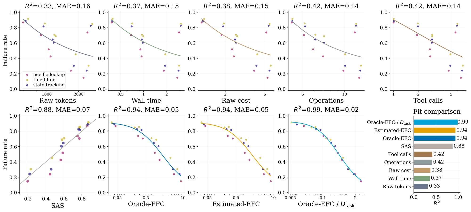
$**Figure 1:** **Controlled scaling comparison on synthetic tasks.** The first nine panels, read left to right and top to bottom, fit the common power-law failure model to raw tokens, wall time, raw cost, operations, tool calls, SAS, Oracle-EFC, Estimated-EFC, and Oracle-EFC/ $D_{\mathrm{task}}$. Points are aggregated failure rates across task families and harnesses, and curves are fitted trends. The final panel summarizes the corresponding $R^2$ values, showing that demand-normalized Oracle-EFC gives the strongest curve collapse.$

Figure 1 separates three increasingly informative descriptions of a trajectory. (i) Raw expenditure is a weak scaling coordinate. Raw tokens, wall-clock time, and raw cost reach only $R^2=0.33$, $0.37$, and $0.38$, respectively. Moving from aggregate spending to interaction counts helps only modestly: operations and tool calls both reach $0.42$. Thus, the failure curve is not determined by how much budget is spent, nor by how many interaction opportunities are counted. (ii) Feedback-aware coordinates capture the missing signal. SAS improves substantially to $R^2=0.88$, but Oracle-EFC and Estimated-EFC both reach $0.94$, with lower MAE. The fact that Estimated-EFC matches Oracle-EFC closely indicates that the useful-feedback signal can be recovered from trace-time evidence rather than requiring hidden task state. (iii) Task normalization removes the remaining scale mismatch. Oracle-EFC/ $D_{\mathrm{task}}$ reaches $R^2=0.99$ and MAE $0.02$, supporting the view that the relevant scaling coordinate is not absolute feedback alone, but feedback measured relative to task demand.

4.2 Matched Budgets Isolate Feedback Quality

A high-EFC trajectory might appear better simply because it spends more raw compute. To remove this confound, we construct matched-budget pairs on the same task and model. The two conditions share the same token budget, tool-call budget, wall-clock budget, operation count, and raw-cost accounting, but differ only in the quality of feedback returned to the harness. The low-quality condition produces noisy, redundant, and weakly retained observations, whereas the high-quality condition produces targeted, valid, non-redundant feedback that updates the agent state.

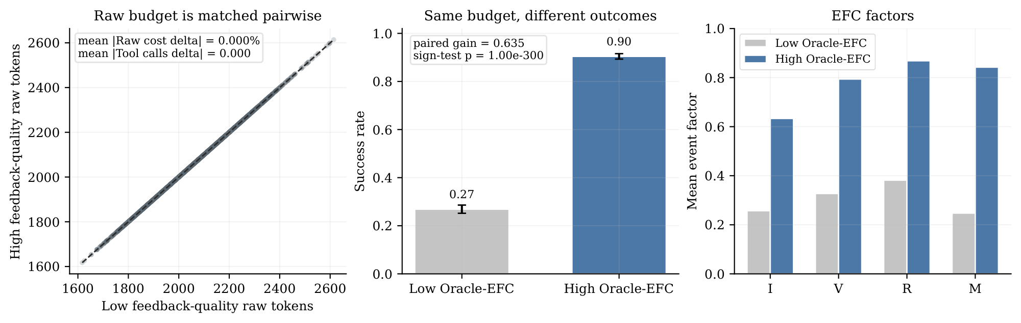
Figure 2 turns the scaling correlation into a matched-budget intervention. (i) Success changes even when raw budget is fixed. The pairwise budget panel collapses onto the diagonal, with mean absolute raw-cost delta $0.000%$ and mean tool-call delta $0.000$, yet the high-feedback-quality condition increases success from $0.27$ to $0.90$ ($p=1.$ 0 x 10^-300). This rules out the explanation that the gain comes from spending more compute. (ii) The gain comes from better raw-to-EFC conversion. Informativeness, validity, non-redundancy, and memory update all increase together, which matters because Equation 3 has bottleneck behavior. Feedback contributes little if it is invalid, redundant, irrelevant, or not retained. Thus, the same raw budget succeeds when it is converted into higher-quality effective feedback.

4.3 Trace-Time Estimation Recovers Oracle-EFC

Oracle-EFC requires hidden-state access and is therefore available only in controllable environments. For real trajectories, EFC must be estimated from signals observed before the final outcome is known. We train an event-level Estimated-EFC model on synthetic calibration tasks using only trace-time features, including checker use, checker scope, tool-result references, plan updates, memory retention, repeated-error avoidance, observation consistency, subgoal progress, and trace position. The final success label is not used as an input.

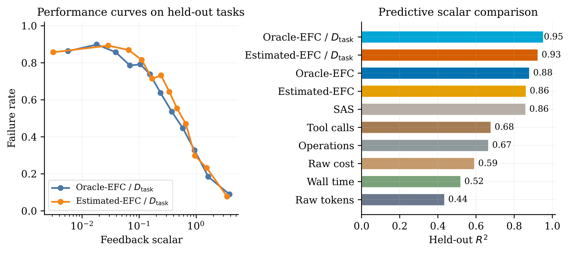
$**Figure 3:** **Trace-time Estimated-EFC on held-out tasks.** Left: Estimated-EFC/ $D_{\mathrm{task}}$ closely follows the held-out failure curve of Oracle-EFC/ $D_{\mathrm{task}}$. Right: the held-out $R^2$ ranking shows that the trace-time estimator nearly matches the oracle coordinate and outperforms raw-compute baselines and SAS.$

Figure 3 addresses whether EFC is only an oracle diagnostic. (i) Estimated-EFC recovers most of the oracle feedback coordinate before the final outcome is observed. Without task normalization, Estimated-EFC reaches $R^2=0.86$, close to Oracle-EFC at $0.88$ and comparable to SAS. (ii) Demand normalization improves oracle and estimated coordinates in the same direction. Estimated-EFC/ $D_{\mathrm{task}}$ and Oracle-EFC/ $D_{\mathrm{task}}$ rise to $0.93$ and $0.95$, respectively, while raw-compute baselines remain much weaker, ranging from raw tokens at $0.44$ to tool calls at $0.68$. This matched improvement shows that trace-time evidence captures useful feedback, and that $D_{\mathrm{task}}$ removes residual task-family scale differences rather than merely re-ranking runs after the fact.

4.4 Executable Code Tasks Preserve the EFC Signal

We next test whether the trace-time EFC signal survives in a more realistic code-execution setting. We use held-out executable programming tasks in a HumanEval-like function-completion format, where candidate programs are checked against executable tests and repaired over multiple attempts. The harness observes syntax errors, runtime errors, unit-test failures, partial correctness signals, and subsequent repair behavior. Estimated-EFC is computed only from these trace-time signals, while oracle quantities are used only for diagnostic comparison. We also evaluate seven harness variants and report estimated feedback efficiency, $\widehat{\eta}=\widehat{\mathrm{EFC}}/C_{\mathrm{raw}}$, measuring how much Estimated-EFC is produced per unit of raw cost.

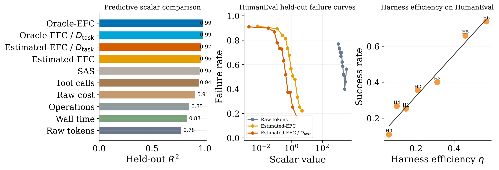
$**Figure 4:** **Executable code tasks preserve the EFC signal.** Left: on held-out executable programming tasks, EFC-based predictors achieve the highest predictive $R^2$, with Estimated-EFC/ $D_{\mathrm{task}}$ reaching $0.97$ and raw tokens reaching $0.78$. Middle: failure curves for Estimated-EFC and Estimated-EFC/ $D_{\mathrm{task}}$ are cleaner than the raw-token curve, indicating that execution feedback quality is more informative than generation length. Right: harness success increases with estimated feedback efficiency, showing that harness variants succeed when they convert raw budget into effective feedback more efficiently.$

Figure 4 shows that the EFC signal persists in executable code tasks. (i) Tool calls become a strong raw baseline when they partially align with executable feedback. Since tool calls often run tests that expose syntax errors, runtime errors, or unit-test failures, they reach $R^2=0.94$, far above raw tokens at $0.78$ and close to SAS at $0.95$. (ii) EFC-based coordinates remain stronger because they score what the tests reveal and whether the harness uses that information. Estimated-EFC reaches $0.96$, Estimated-EFC/ $D_{\mathrm{task}}$ reaches $0.97$, and oracle variants reach $0.99$. (iii) Feedback efficiency explains harness-level differences. Shallow or noisy harnesses remain low-success even when they spend budget, while H5 and H6 achieve the highest success by converting raw cost into higher estimated feedback efficiency $\widehat{\eta}=\widehat{\mathrm{EFC}}/C_{\mathrm{raw}}$. Thus, executable feedback strengthens the interpretation that tool use helps when it produces useful, retained evidence, not merely because it increases interaction count.

(i) Raw budget is not the scaling coordinate for agent harnesses. Across controlled scaling and matched-budget interventions, raw-compute scalars explain only part of the performance trend, and success can change sharply even when raw cost, tokens, operations, and tool calls are fixed. (ii) The predictive signal lies in raw-to-EFC conversion. Scalars become stronger as they move from aggregate expenditure toward feedback opportunities, but EFC-based coordinates remain stronger because they account for whether feedback is informative, valid, non-redundant, and retained. (iii) EFC is not merely an oracle diagnostic.

Trace-time estimation recovers most of the oracle coordinate before the final outcome is observed, and executable code tasks preserve the same signal even when tool calls are already competitive. Together, these results support EFC, normalized by task demand when needed, as the scaling coordinate for agent harness performance.

5. Decomposing EFC: Harness Efficiency and Task Demand

Section Summary: This section decomposes effective feedback compute (EFC) into two parts: harness efficiency, which shows how much useful feedback a system extracts from a given raw compute budget, and a task-normalized measure that compares the feedback received against what the task actually needs. Harness factors such as stronger verifiers, better routers, and reliable memory boost efficiency and raise success rates, while interface problems like noise or complex tools lower it; experiments confirm these gains come from better conversion rather than simply spending more compute. Task demand, shaped by factors like reasoning depth and state complexity, sets the scale at which feedback becomes sufficient, so even efficient harnesses can fail on harder tasks that require more total EFC.

Section 4 identifies EFC as a stronger scaling coordinate than raw compute. We now decompose this coordinate into two mechanisms. The first is harness efficiency,

$ \eta = \frac{\mathrm{EFC}}{C_{\mathrm{raw}}},\tag{16} $

which measures how much effective feedback a harness extracts per unit of raw budget. For trace-estimated and real-trace variants, the numerator is replaced by $\widehat{\mathrm{EFC}}$ or nonredundant stable EFC (NRS-EFC), respectively. The second is the task-normalized feedback variable,

$ X = \frac{\mathrm{EFC}}{D_{\mathrm{task}}},\tag{17} $

which measures whether the extracted feedback is sufficient relative to task demand. This section separates the two mechanisms: harness design controls raw-to-EFC conversion through $\eta$, while task demand controls the scale on which feedback becomes sufficient through $D_{\mathrm{task}}$.

5.1 Harness Factors Control Raw-to-EFC Conversion

We first vary individual harness and environment factors in controlled synthetic tasks while keeping the task distribution and budget accounting fixed. The positive harness factors are verifier strength, router quality, and memory fidelity; the adverse interface factors are tool entropy, state pressure, and observation noise. For each factor, we compare low, medium, and high levels and measure the induced change in harness efficiency $\eta=\mathrm{EFC}/C_{\mathrm{raw}}$ and the corresponding success rate.

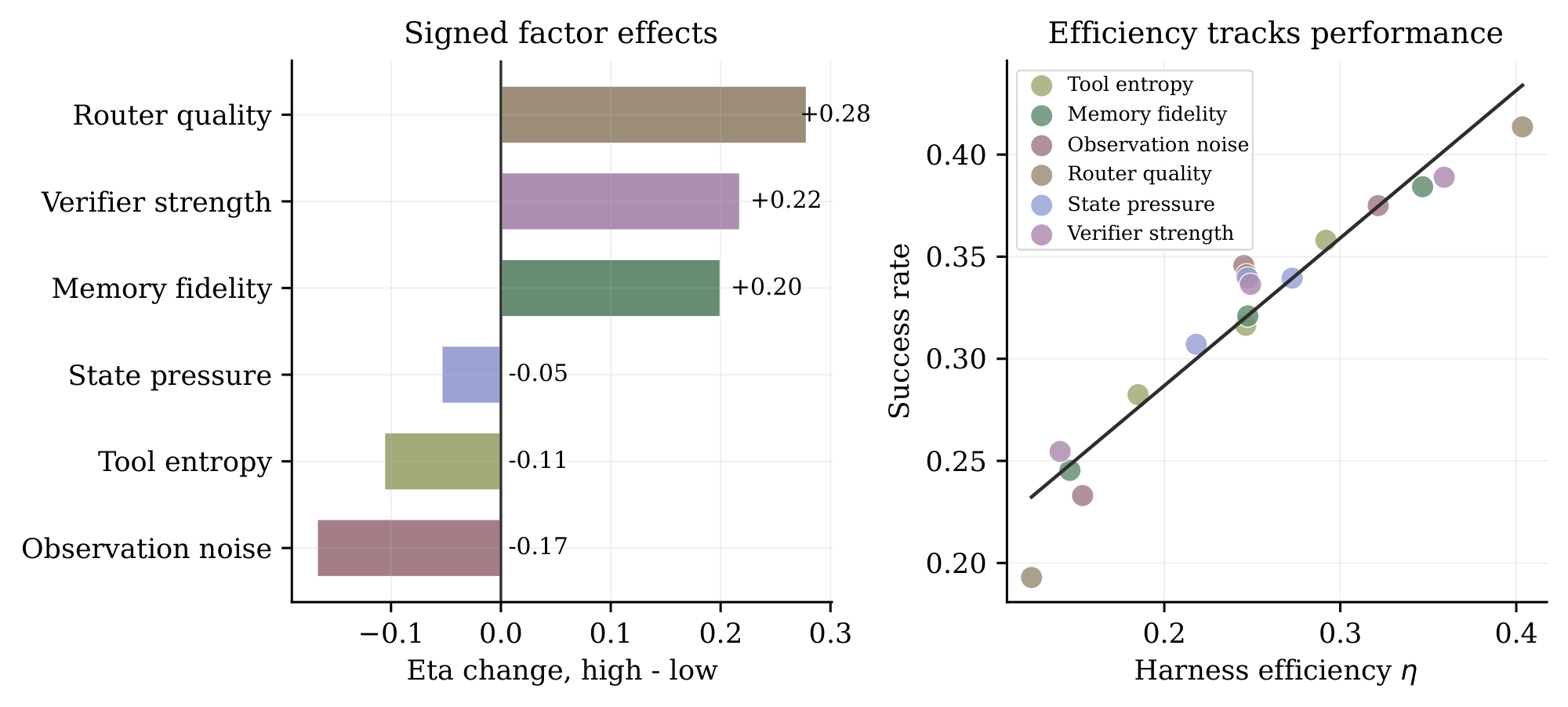
$**Figure 5:** **Harness factors control raw-to-EFC conversion.** Left: signed high-minus-low effects on $\eta$ show that router quality, verifier strength, and memory fidelity increase efficiency, whereas observation noise, tool entropy, and state pressure reduce it. Right: success rate tracks harness efficiency across factor settings, indicating that these design and interface changes affect performance primarily by changing how much effective feedback is extracted from the same raw budget.$

Figure 5 shows that the same raw budget can be converted into very different amounts of effective feedback. (i) The largest gains come from factors that improve the selection and reliability of feedback. Router quality gives the largest efficiency gain ($+0.28$), followed by verifier strength ($+0.22$) and memory fidelity ($+0.20$). This ordering is consistent with Equation 3: routing improves relevance and non-redundancy, verification improves validity, and memory improves retention. (ii) Interface frictions reduce efficiency by corrupting or diluting feedback. Observation noise produces the largest drop ($-0.17$), tool entropy also reduces efficiency ($-0.11$), and state pressure has a smaller negative effect ($-0.05$). (iii) Outcomes track conversion rather than budget alone. Success rises approximately monotonically with $\eta$, from about $0.19$ at the least efficient settings to above $0.40$ at the most efficient settings. Thus, these factors affect performance by changing the raw-to-EFC conversion rate.

5.2 Module Ablations Localize Raw-to-EFC Conversion Gains

We next localize the raw-to-EFC conversion gains to concrete harness components. We ablate three harness modules and one interface corruption factor: verifier strength, memory fidelity, router quality, and observation noise. Each family is evaluated at ordered settings, ranging from disabled or weak configurations to stronger configurations that provide more reliable feedback. We measure both harness efficiency $\eta=\mathrm{EFC}/C_{\mathrm{raw}}$ and downstream success.

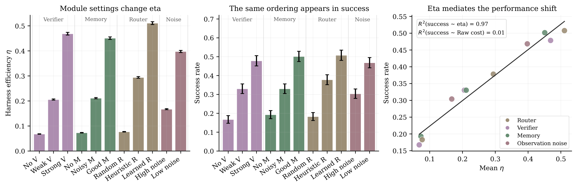
$**Figure 6:** **Module ablations localize raw-to-EFC conversion gains.** Left: stronger verifier, memory, and router modules increase harness efficiency $\eta$, while lower observation noise also improves $\eta$. Middle: the same ordering appears in success rate, showing that module improvements that increase $\eta$ also improve task outcomes. Right: success is almost fully explained by mean $\eta$ ($R^2=0.97$), whereas raw cost has essentially no explanatory power ($R^2=0.01$), indicating that $\eta$ mediates the performance shift.$

Figure 6 shows that raw-to-EFC conversion can be localized to specific harness modules. (i) The ablations produce a dose-response pattern. Moving from disabled or weak modules to stronger verifier, memory, and router settings increases both $\eta$ and success, while reducing observation noise produces the same direction of improvement. Router quality reaches the highest mean $\eta$ and success among the module settings, matching the factor scan in Figure 5. (ii) Harness efficiency mediates the performance shift, while raw cost does not. Across module settings, mean $\eta$ explains almost all variation in success ($R^2=0.97$), whereas raw cost explains almost none ($R^2=0.01$). This localizes the mechanism: modules help when they improve validity, retention, relevance, non-redundancy, or observation quality, not when they merely change expenditure.

5.3 Task Demand Sets the Required EFC Scale

A harness can convert raw budget into EFC efficiently and still fail when the task requires more feedback than the trajectory provides. We therefore test whether task demand provides the scale needed to compare EFC across task families. In controlled needle lookup, rule filtering, and state tracking tasks, we evaluate raw compute baselines, SAS, raw Oracle-EFC, and two demand-normalized Oracle-EFC coordinates under the same power-law failure model. The hand-designed demand is

$ D_{\mathrm{task}}

L \cdot H_{\mathrm{tool}} \cdot S_{\mathrm{state}} \cdot (1 + N_{\mathrm{obs}}) \cdot (1 - V_{\mathrm{oracle}}),\tag{18} $

where longer reasoning depth, higher tool entropy, larger state pressure, noisier observations, and lower verifier-signal coverage all increase task demand. The fitted variant uses the same task-demand factors but estimates their relative exponents from calibration tasks.

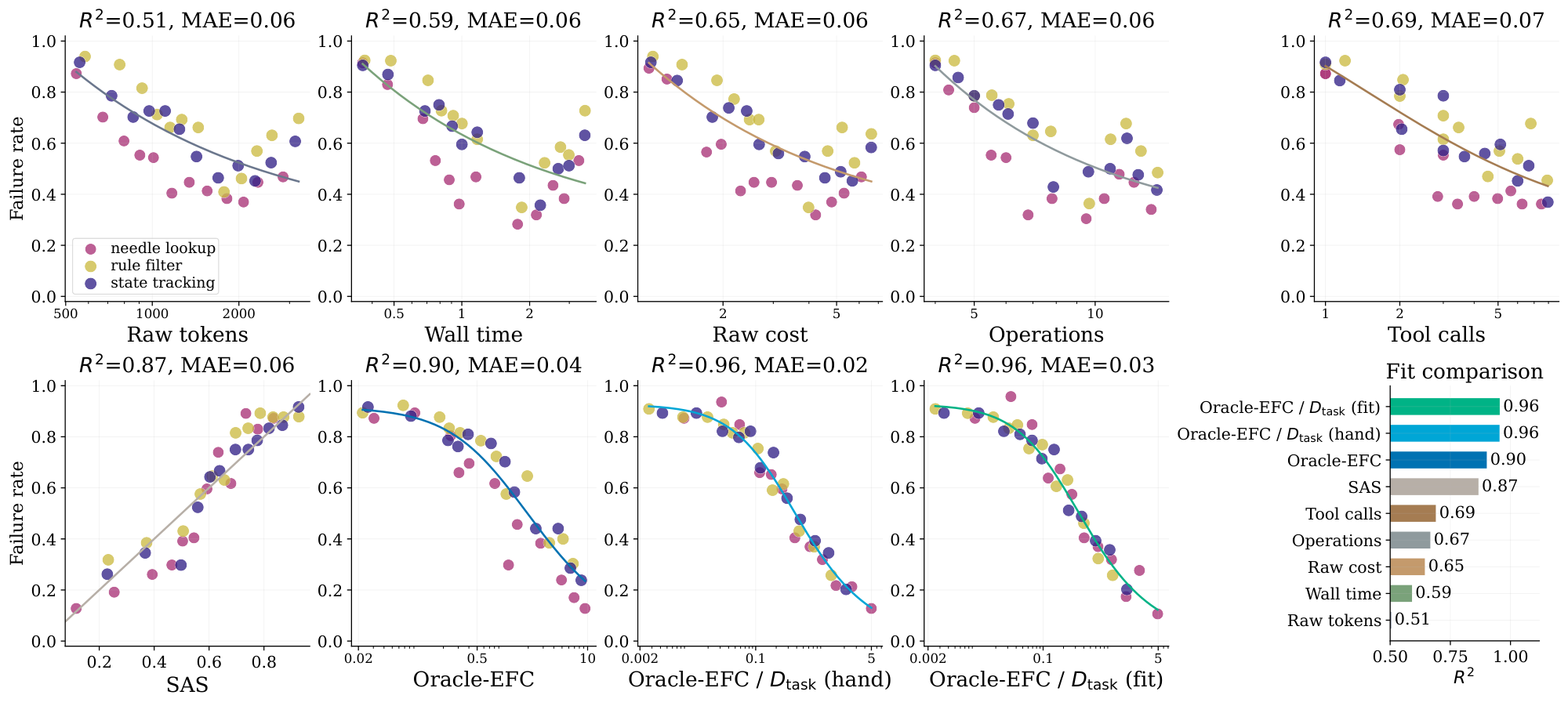
Figure 7 shows that task demand is the missing scale factor for cross-family prediction. (i) Absolute raw budget cannot align task families. Raw compute baselines improve as they move closer to interaction opportunities, from raw tokens at $R^2=0.51$ to tool calls at $0.69$, and SAS reaches $0.87$. Raw Oracle-EFC improves further to $0.90$, but the task families still show residual offsets, indicating that the same amount of effective feedback is not equally sufficient across needle lookup, rule filtering, and state tracking. (ii) Dividing EFC by task demand removes this residual scale mismatch. Oracle-EFC/ $D_{\mathrm{task}}$ reaches $R^2=0.96$ with both hand-designed and fitted task demand, with MAE $0.02$ and $0.03$, respectively. The similar performance of the two normalizations shows that the key requirement in these controlled families is the denominator itself: EFC must be measured relative to the amount of feedback the task requires.

5.4 Task-Demand Calibration Transfers to Mixed Holdout

We finally test whether task-demand normalization transfers beyond the controlled task families used to motivate it. We evaluate a mixed held-out set with heterogeneous task structure and compare raw compute baselines, SAS, NRS-EFC, hand-designed NRS-EFC/ $D_{\mathrm{task}}$, and fitted NRS-EFC/ $D_{\mathrm{task}}$. The fitted task-demand model uses the same factors as before, including reasoning depth, tool entropy, state pressure, observation noise, and verifier-signal coverage, but learns their exponents on a calibration split and evaluates the resulting scaling coordinate on unseen tasks.

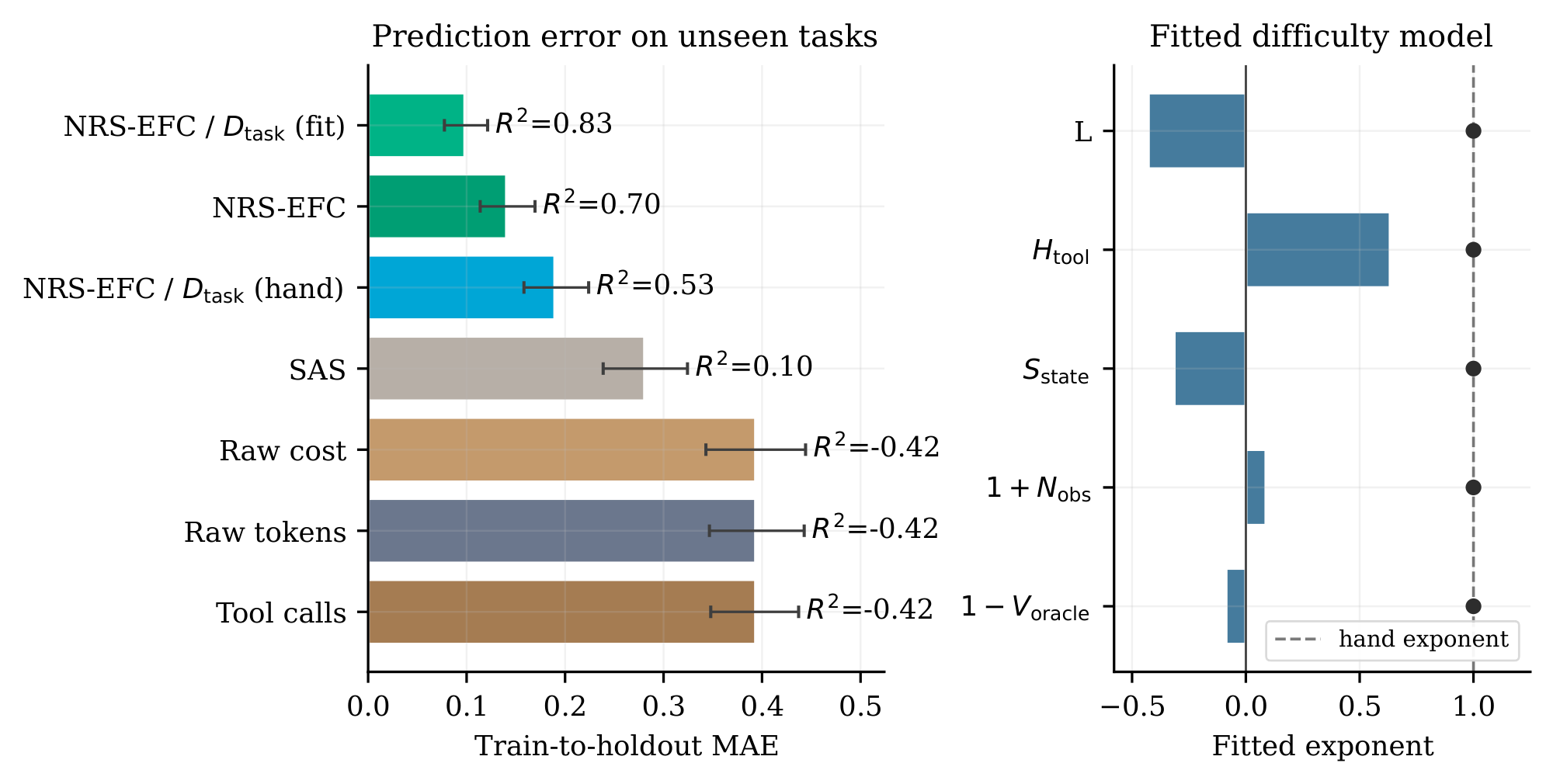
$**Figure 8:** **Task-demand calibration transfers to mixed held-out tasks.** Left: prediction error on unseen tasks compares raw tokens, tool calls, raw cost, SAS, NRS-EFC, hand-designed NRS-EFC/ $D_{\mathrm{task}}$, and fitted NRS-EFC/ $D_{\mathrm{task}}$. The fitted task-demand normalization gives the lowest train-to-holdout MAE and the highest held-out $R^2$. Right: the fitted task-demand model learns non-uniform exponents over demand factors rather than using the fixed hand exponent, showing that mixed tasks require calibrated weighting of demand components.$

Figure 8 shows that task-demand calibration improves the portability of the EFC coordinate. (i) Raw compute does not transfer on unseen mixed tasks. Raw tokens, tool calls, and raw cost cluster around train-to-holdout MAE $0.39$ with held-out $R^2=-0.42$, while SAS improves to MAE about $0.28$ and $R^2=0.10$. NRS-EFC is substantially stronger, reaching MAE about $0.14$ and $R^2=0.70$, which shows that trace-derived nonredundant and retained feedback carries the transfer signal. (ii) Task-demand normalization must be calibrated in heterogeneous settings. The hand-designed denominator gives MAE about $0.19$ and $R^2=0.53$, which is weaker than raw NRS-EFC, indicating that equal exponents are poorly matched to this mixed holdout. The fitted denominator gives the best result, reducing MAE to about $0.10$ and increasing held-out $R^2$ to $0.83$. (iii) The fitted exponents should be read as calibration weights, not universal causal signs. The model upweights tool entropy, downweights reasoning depth and state pressure, and assigns smaller corrections to observation noise and verifier-signal coverage. Thus, calibration preserves the conceptual role of $D_{\mathrm{task}}$ while adapting its scale to the held-out task mixture.

(i) Harness design controls raw-to-EFC conversion. Factor scans and module ablations show that routing, verification, memory, and cleaner observations improve performance mainly by increasing harness efficiency $\eta$, not by increasing raw expenditure. (ii) Task demand controls sufficiency.

Absolute EFC is stronger than raw compute, but cross-family prediction improves when EFC is measured relative to $D_{\mathrm{task}}$. (iii) Calibration is needed when task mixtures are heterogeneous. Hand-designed task demand is effective in controlled families, while fitted task-demand normalization gives the best transfer on mixed held-out tasks. Together, these results explain why raw budget alone is insufficient: successful harnesses must both extract more effective feedback per unit budget and measure that feedback against the right task scale.

6. Held-Out and Prospective Validation

Section Summary: The section tests whether the EFC scaling relationship holds up when applied to new situations not used in the original model fitting. Across held-out task types, harnesses, models, and real-world execution traces, normalizing feedback by task demand consistently predicted success rates more accurately than raw compute or other baselines, with the advantage clearest when decision policies changed. Harness efficiency also proved highly specific to each kind of task rather than a fixed property, confirming that what matters is useful feedback relative to difficulty, not simply spending more resources.

The previous sections identify EFC as the scaling coordinate and decompose it into harness efficiency and task demand. We now test whether this coordinate generalizes beyond the configurations used to fit the scaling curves. We consider three validation settings. First, we hold out task families, harness variants, models, and combined configurations. Second, we evaluate heterogeneous real execution traces using nonredundant stable EFC (NRS-EFC). Third, we evaluate a prospective batch of new real traces under a prediction protocol specified before the batch is collected and scored. Across these settings, the central question is whether success is predicted by task-demand-normalized feedback rather than by raw expenditure.

6.1 Task-Demand-Normalized EFC Predicts Unseen Configurations

We evaluate held-out prediction by removing configurations along four axes: task family, harness variant, model, and combined setting. For each split, we fit the power-law scaling model on the remaining configurations in failure-rate space, consistent with Equation 13. For visualization and calibration analysis, we report the equivalent success-rate prediction $1-\widehat{E}(z)$ on the held-out group. We compare raw compute baselines, SAS, task-demand-normalized Oracle-EFC, and task-demand-normalized Estimated-EFC. The task-demand denominator is either hand-designed from task-demand factors or fitted on the training split. Estimated-EFC is computed only from trace-time signals.

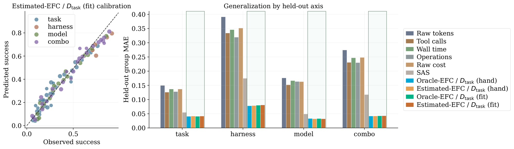
$**Figure 9:** **Task-demand-normalized EFC predicts unseen configurations.** Left: predicted success, computed as $1-\widehat{E}(z)$ from the fitted failure-rate scaling model, is calibrated against observed success across held-out task, harness, model, and combined splits. Right: grouped bars report held-out group MAE for raw compute baselines, SAS, and task-demand-normalized EFC coordinates across the four held-out axes. Task-demand-normalized EFC gives the lowest prediction error across all axes.$

Figure 9 shows that the EFC coordinate transfers across unseen axes rather than only fitting pooled correlations. (i) Calibration is preserved at the level of absolute success after converting the fitted failure-rate predictions to success rates. The left panel stays close to the diagonal across task, harness, model, and combined splits, which indicates that fitted Estimated-EFC/ $D_{\mathrm{task}}$ predicts success rates rather than only ranking configurations. (ii) The coordinate ordering is stable across held-out axes. Raw-compute scalars have the largest errors, SAS reduces error, and task-demand-normalized EFC forms the lowest-error group on every split. The gain is largest on harness and combined splits, where raw expenditure is most confounded by changed decision policies. (iii) Fitted and hand-designed task demand are close. Their similar errors show that the transfer signal mainly comes from measuring feedback relative to task demand, while fitting improves calibration under distribution shift.

6.2 Non-Redundant Stable EFC Reveals Slice-Specific Harness Efficiency

We next evaluate whether the same feedback-based scaling picture survives on real execution traces, where observations are noisier, errors are often repeated, and intermediate states are less controlled than in the synthetic and semi-realistic settings. We therefore use nonredundant stable EFC (NRS-EFC), which keeps feedback events that are both informative and retained, while down-weighting redundant or unstable signals that do not contribute durable progress. We pool heterogeneous real slices, including HumanEval-style code generation, terminal interaction, and SWE tasks, and compare raw compute baselines, SAS, NRS-EFC, and NRS-EFC/ $D_{\mathrm{task}}$ under the same aggregated scaling protocol. We also examine harness efficiency $\eta = \mathrm{EFC}/C_{\mathrm{raw}}$ using NRS-EFC in order to understand how different harnesses convert raw budget into effective feedback on each real slice.

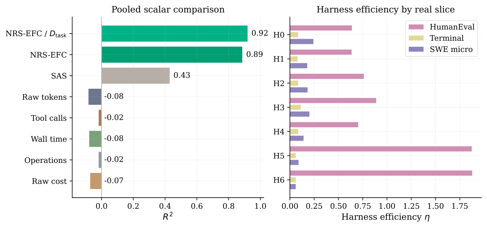
$**Figure 10:** **Nonredundant stable EFC reveals slice-specific harness efficiency.** Left: pooled scalar comparison on mixed real traces, reporting predictive $R^2$ for raw compute baselines, SAS, NRS-EFC, and NRS-EFC/ $D_{\mathrm{task}}$. Demand-normalized NRS-EFC gives the strongest pooled fit, followed closely by raw NRS-EFC, while raw compute baselines fail to provide a reliable pooled scaling coordinate. Right: harness efficiency $\eta$ computed from NRS-EFC is shown for H0–H6 across HumanEval, Terminal, and SWE slices. The absolute efficiency scale and the ordering of harnesses vary substantially by slice, showing that harness efficiency is task-dependent rather than a fixed global property.$

Figure 10 shows three main results. (i) Raw compute largely fails as a pooled predictor on heterogeneous real traces: raw tokens and wall time both obtain $R^2=-0.08$, raw cost reaches $-0.07$, and tool calls and operations each remain at $-0.02$. This contrasts sharply with NRS-EFC, which reaches $R^2=0.89$, and NRS-EFC/ $D_{\mathrm{task}}$, which further improves to $0.92$. SAS is substantially better than raw compute at $0.43$, but it still falls far short of the feedback-based coordinates. Thus, in realistic mixed settings, simply spending more budget is not predictive of success; what matters is whether the trajectory accumulates nonredundant, retained feedback, and whether that feedback is large enough relative to task demand. (ii) The right panel shows that harness efficiency is strongly slice-specific rather than globally fixed. On HumanEval, later harnesses H5 and H6 dominate with $\eta $ $\approx 1$ $.9$, far above earlier variants, indicating that richer verification and feedback exploitation translate into much more effective progress on executable coding tasks. On Terminal, all harnesses remain at very low efficiency, roughly around $0.1$, suggesting that the slice is intrinsically hard to convert into clean, reusable feedback. On SWE, the pattern changes again: earlier or mid-stage harnesses perform best, with H0 and H3 among the strongest, while H5 and H6 no longer dominate. This reversal indicates that the best harness design depends on the structure of the environment and the type of feedback available. Overall, these results support the view that NRS-EFC captures the relevant scaling signal on real tasks, while $\eta$ should be understood as a harness–task interaction rather than as an invariant property of the harness alone.

6.3 Prospective Holdout Validates the Scaling Coordinate

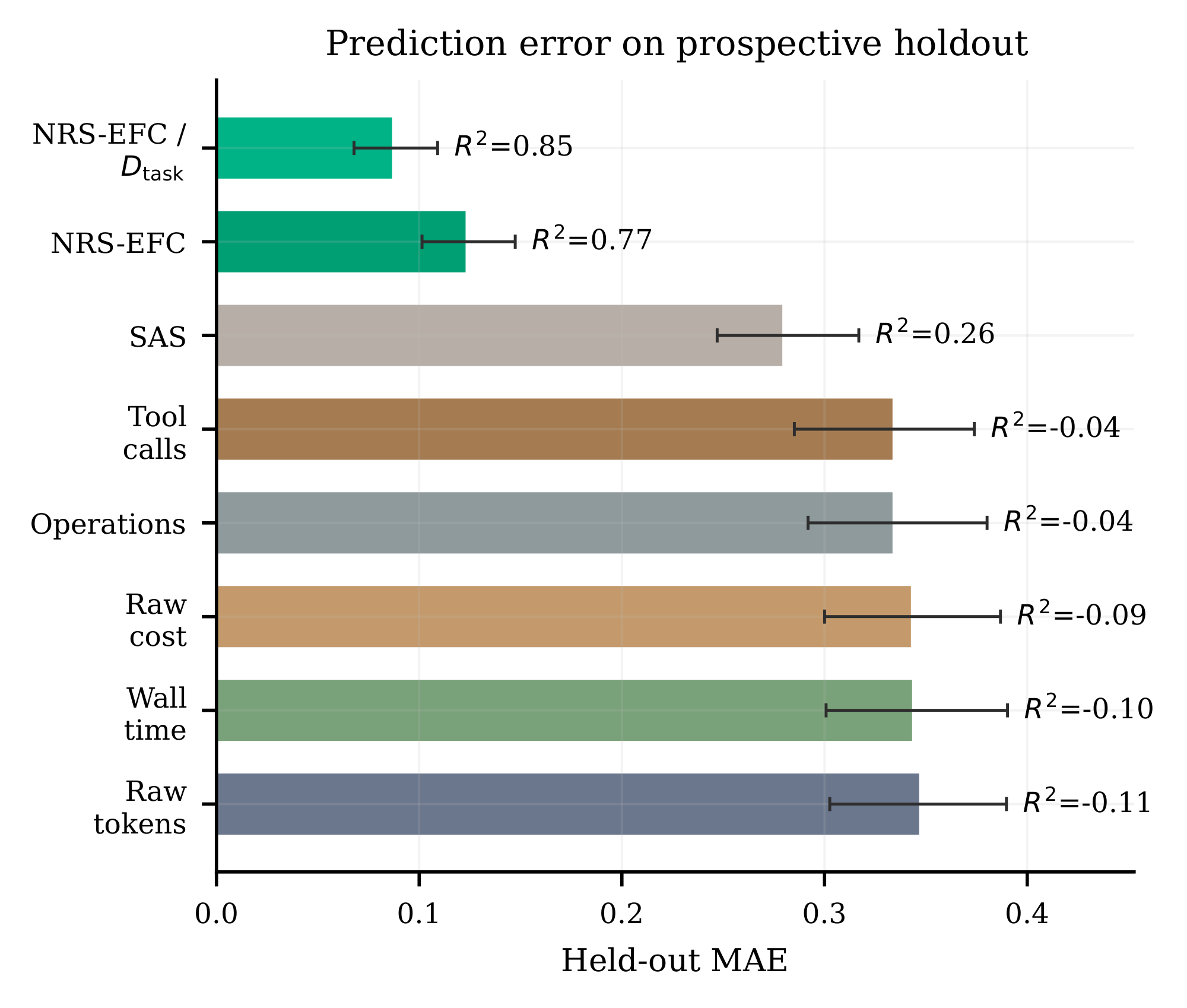
$**Figure 11:** **Prospective holdout prediction.** Bars report held-out MAE on a prospective batch of unseen real traces, and text annotations report the corresponding held-out $R^2$. NRS-EFC/ $D_{\mathrm{task}}$ gives the best prospective prediction, followed closely by raw NRS-EFC, while raw compute baselines and SAS are substantially weaker.$

We conclude with a prospective holdout test that evaluates whether the same coordinate transfers to traces that were not available during metric design or calibration. Before collecting the prospective runs, we fixed the prediction protocol, including the definition of NRS-EFC, the task-demand factors, the fitted task-demand exponents, and all comparison baselines. We then evaluate a new held-out batch of real traces and compare raw compute baselines, SAS, NRS-EFC, and NRS-EFC/ $D_{\mathrm{task}}$ using the same held-out prediction procedure as above. This setting asks whether a prespecified feedback-based coordinate remains predictive when both the task mix and the evaluation examples are unseen.

Figure 11 shows that the ordering observed in earlier validation settings transfers to the prospective batch. (i) Feedback-based coordinates remain predictive on new real traces. NRS-EFC/ $D_{\mathrm{task}}$ achieves the best held-out prediction, with the highest held-out $R^2$ of $0.85$, while raw NRS-EFC follows closely at $0.77$. SAS remains informative but is substantially weaker at $R^2=0.26$. (ii) Raw expenditure is not a reliable out-of-sample coordinate. Raw tokens, tool calls, wall time, operations, and raw cost all obtain negative held-out $R^2$, indicating that they perform worse than a mean predictor on the prospective batch. (iii) Task-demand normalization provides a targeted calibration gain rather than an evaluation-set-specific adjustment. NRS-EFC already captures nonredundant retained feedback, and dividing by $D_{\mathrm{task}}$ improves prediction when the prospective batch mixes tasks with different feedback requirements. Because the coordinate and calibration procedure were specified before evaluating the prospective batch, the improvement supports the proposed scaling coordinate rather than post hoc adaptation to the held-out examples.

(i) The EFC coordinate generalizes across held-out axes. Task-demand-normalized Oracle-EFC and Estimated-EFC predict unseen task families, harness variants, models, and combined configurations more accurately than raw compute baselines or SAS. (ii) Real traces require stable nonredundant feedback. NRS-EFC filters repeated or unstable observations and restores a strong pooled scaling signal, while slice-specific $\eta$ shows that harness efficiency is a harness–task interaction. (iii) Prospective validation provides an additional check against post hoc metric tuning. With the metric family, task-demand factors, and calibration procedure specified before evaluation, NRS-EFC/ $D_{\mathrm{task}}$ remains the best predictor on new real traces.

Together, these results show that a predictive scaling law for agent harnesses must account for both raw-to-EFC conversion and task demand.

7. Related Work

Section Summary: Previous research on scaling laws has linked language-model gains to larger models, more data, and greater training compute, while newer studies explore how extra computation at inference time—through repeated sampling, search, or revision—can further boost results. A separate line of work examines “agent harnesses,” the surrounding systems that add reasoning, verification, and feedback loops, showing that overall performance often depends on jointly scaling the model and this supporting infrastructure rather than model size alone. The present section positions EFC as a complementary, scalar measure that isolates how much useful feedback is actually retained, distinguishing it from raw compute counts or existing system-level baselines such as SAS.

Scaling and test-time compute.

Scaling laws connect language-model performance with model size, data size, and training compute ([5, 6]). Recent work extends this view to inference-time computation, showing that repeated sampling, search, revision, and adaptive allocation can improve performance when additional test-time budget is available ([7, 8, 9, 10]). These studies establish test-time compute as an important scaling axis, but they usually measure compute through samples, tokens, rollouts, or search budget. Our work instead asks which scalar predicts when this extra computation becomes useful. EFC answers this by counting feedback that is informative, valid, non-redundant, and retained, then normalizing it by task demand.

Harness feedback and system scaling.

Agent harnesses improve language models by adding reasoning, action, verification, search, memory, and iterative feedback ([11, 12, 13, 14, 15, 16]). Recent work increasingly treats the harness itself as a first-class object of design and evaluation, including natural-language harness representations, versioned agent-optimization loops, and context-retrieval benchmarks for coding agents ([17, 18, 19]). System-level studies further argue that agent performance depends on the joint scaling of model capability, orchestration, verification, coordination, and overhead rather than on base-model scale alone ([1, 20]). These works motivate harness-level scaling, while our focus is complementary: we seek a trace-level scalar coordinate that separates raw expenditure from useful retained feedback. EFC therefore provides a compact predictive quantity for closed-loop harness scaling and is directly compared with SAS as a strong system-level baseline.

8. Conclusion

Section Summary: This paper argues that the performance gains of AI agent systems come less from simply spending more raw computing power during operation and more from generating high-quality, useful feedback that directly helps solve the task. The authors introduce a new measurement called Effective Feedback Compute to track how much valid and non-redundant feedback an agent actually receives, after adjusting for how hard each task is. Their experiments across many settings show this measure predicts success better than tracking tokens, time, or cost alone, suggesting future agent designs should focus on turning limited resources into durable, task-relevant feedback rather than increasing spend.

This paper argues that the scaling behavior of agent harnesses is better explained by effective feedback than by raw test-time expenditure. We introduced Effective Feedback Compute (EFC), a trace-level coordinate that measures the amount of valid, relevant, non-redundant, and retained feedback available to a harness, together with task-demand normalization for comparing heterogeneous tasks. Across controlled simulations, executable code tasks, real mixed traces, held-out splits, and a prospective validation batch, EFC-based coordinates consistently outperform raw-compute baselines such as tokens, tool calls, operations, wall time, and cost, and also improve over a strong SAS baseline. The experiments further show that harness interventions primarily matter by changing how efficiently raw budget is converted into durable feedback: under matched raw budgets, improving feedback quality substantially increases success, while normalized EFC produces the strongest curve collapse across task difficulty. These results suggest that agent-system scaling should be understood not simply as spending more inference-time compute, but as accumulating sufficient effective feedback relative to task demand. Future work should extend EFC estimation to broader open-ended environments, improve task-demand calibration, and use EFC as an objective for adaptive budget allocation and harness design.

Appendix

Section Summary: The appendix outlines three progressively realistic layers of tasks used to evaluate agent performance and feedback measurement. The synthetic layer uses procedurally generated problems with known hidden states for controlled testing and calibration of progress metrics. The semi-realistic and real-benchmark layers incorporate executable code or tool-use tasks and filtered public benchmarks, respectively, to assess whether the same metrics remain reliable amid natural model errors, noisy observations, and incomplete verification, while also detailing how task difficulty and event logs are computed.

A. Task Details

This appendix describes the task layers used in our experiments. The purpose of the task suite is not to maximize benchmark coverage, but to span a controlled range from oracle-observable feedback to realistic agent trajectories.

A.1 Synthetic Controllable Tasks

The synthetic layer contains procedurally generated tasks with hidden state and known ground-truth solution paths. Each task instance specifies a target state, a set of candidate hypotheses, a tool interface, and a deterministic evaluator. Because the latent state is known to the experimenter, we can compute Oracle-EFC for each feedback event.

We use this layer for three purposes. First, it provides controlled variation in task demand, including required solution length, tool-selection entropy, state size, observation noise, and verifier availability. Second, it allows us to test whether feedback events measured by EFC correspond to real progress toward the solution. Third, it provides calibration data for Estimated-EFC, which is later applied to tasks where oracle state is unavailable.

Each synthetic task is generated from a template family. Template parameters control the number of latent variables, the number of distractor tools, the probability of noisy observations, and the coverage of deterministic checkers. We split generated tasks into calibration and held-out sets by template family and random seed.

A.2 Semi-Realistic Executable Tasks

The semi-realistic layer contains tasks with realistic artifacts and executable checkers. Examples include small code-repair tasks, data-analysis tasks, and tool-use tasks with deterministic validation. These tasks are designed to produce natural agent traces while preserving reliable evaluation.

For code tasks, the final answer is executed against unit tests or reference checks. Intermediate checker results, such as syntax errors, failing tests, and partial correctness signals, are logged as trace observations. For tool-use tasks, the environment exposes a fixed set of tools and records whether tool outputs are later referenced or used in solution updates.

This layer is used to evaluate whether the EFC estimators calibrated on synthetic tasks remain predictive when traces contain realistic model errors, ambiguous observations, and incomplete verification.

A.3 Real Benchmark Subsets

The real benchmark layer uses verifiable subsets of existing agent benchmarks. We include only tasks for which final success can be evaluated automatically and for which traces can be logged in a consistent format. The benchmark layer is used for external validity rather than leaderboard comparison.

We apply the following filtering rules:

the task must have an automatic final evaluator;
the required environment must be reproducible in a local or sandboxed execution setting;
the task must admit meaningful intermediate observations, such as test results, command outputs, or tool responses;
the task must fit within the budget limits used by the harness family.

When a benchmark contains tasks with very large setup cost or unstable external dependencies, we exclude those tasks from the main analysis and report the filtering rule separately. The resulting subset is intended to test scaling-law generalization, not to estimate absolute benchmark performance.

A.4 Task Demand Variables

For each task, we compute a hand-designed task-demand score

$ D_{\mathrm{task}}

L \cdot H_{\mathrm{tool}} \cdot S_{\mathrm{state}} \cdot (1 + N_{\mathrm{obs}}) \cdot (1 - V_{\mathrm{oracle}}). $

The terms are defined as follows:

$L$ is the estimated minimum number of reasoning or action steps.
$H_{\mathrm{tool}}$ measures tool-selection entropy or the number of plausible but incorrect tools.
$S_{\mathrm{state}}$ measures the amount of state that must be tracked across the trajectory.
$N_{\mathrm{obs}}$ measures observation noise, ambiguity, or nondeterminism.
$V_{\mathrm{oracle}}$ measures verifier-signal visibility, namely the availability and coverage of reliable task-level validation signals such as deterministic checkers, explicit tests, partial evaluators, or benchmark scoring hooks.

In real benchmark traces, $V_{\mathrm{oracle}}$ is computed from task metadata about verification coverage rather than from the agent's final outcome or a hidden solution. The agent does not observe oracle answers through this quantity. The factor appears as $1-V_{\mathrm{oracle}}$ because tasks with stronger reliable verification signals require less feedback mass to reach the same effective progress.

All components are normalized within each task layer before forming the product. In addition to this hand-designed score, we also evaluate fitted task-demand weights learned on calibration tasks and applied to held-out tasks.

A.5 Run Logging

For every run, we log the task identifier, task family, harness identifier, model identifier, budget configuration, final success label, raw compute variables, checker outputs, and the full sequence of trajectory events. Each event records the action type, observation type, tool name if applicable, checker result if available, memory update if present, and references to earlier observations. These logs are the sole input to Estimated-EFC on non-oracle tasks.

B. EFC Factor Measurement

This appendix specifies how the event factors $I_t, V_t, R_t, M_t$ are computed or estimated in each task layer. Section 3 defines the common EFC variables and aggregation rules.

B.1 Common Notation

We use $\operatorname{clip}(x)$ to denote clipping to $[0, 1]$:

$ \operatorname{clip}(x)

\min { 1, \max { 0, x } }.\tag{19} $

For every event, the factors are computed before aggregation. The run-level value is then obtained by Equation 4.

When a feature is unavailable in a task layer, we use the closest trace-observable proxy. The final answer correctness label is excluded from all event-level factor estimates.

B.2 Synthetic Controllable Tasks

In the synthetic layer, the experimenter observes the latent task state and the ground-truth solution path. Oracle-EFC therefore uses direct event-level factors. Let $n_t$ denote novelty relative to previous events, $B^{\mathrm{noise}}_t$ the reliability of the observation channel, $B^{\mathrm{route}}_t$ routing quality, $B^{\mathrm{verify}}_t$ verifier strength, and $B^{\mathrm{mem}}_t$ memory fidelity. We instantiate the factors as

$ I_t

\operatorname{clip} \left(B^{\mathrm{route}}_t B^{\mathrm{noise}}_t \Delta^{\mathrm{latent}}_t \right),\tag{20} $

$ V_t

\operatorname{clip} \left(B^{\mathrm{verify}}_t B^{\mathrm{noise}}t V{\mathrm{oracle}} \right),\tag{21} $

$ R_t

\operatorname{clip} \left(n_t B^{\mathrm{route}}_t B^{\mathrm{tool}}_t \right),\tag{22} $

$ M_t

\operatorname{clip} \left(B^{\mathrm{mem}}_t B^{\mathrm{state}}_t (0.82 + 0.18 V_t) \right).\tag{23} $

Here $\Delta^{\mathrm{latent}}_t$ is ground-truth progress toward the target state, $B^{\mathrm{tool}}_t$ discounts high tool ambiguity, and $B^{\mathrm{state}}_t$ discounts memory pressure in large state spaces.

For the three synthetic task families, $\Delta^{\mathrm{latent}}_t$ is defined as follows:

Needle Lookup. Let $C_t$ be the remaining candidate set and let $b_t$ indicate whether the target key-value relation is recovered. We use $\Delta^{\mathrm{latent}}t = \operatorname{clip} ((|C{t-1}|-|C_t|)/\max(1, |C_{t-1}|) + b_t)$.
State Tracking. Let $d_t$ be the number of correct state transitions committed after event $t$ and let $r^{\mathrm{fix}}_t$ indicate correction of a previous state error. We use $\Delta^{\mathrm{latent}}t = \operatorname{clip} ((d_t-d{t-1})/\max(1, L) + r^{\mathrm{fix}}_t)$.
Rule Filter. Let $E_t$ be the number of eliminated nonmatching items and $P_t$ the number of confirmed matching conditions. We use $\Delta^{\mathrm{latent}}t = \operatorname{clip} ((E_t-E{t-1}+P_t-P_{t-1})/\max(1, N_{\mathrm{items}}))$.

The Oracle-EFC event score is

$ \mathrm{EFC}^{\mathrm{oracle}}_t

\kappa I_t V_t R_t M_t.\tag{24} $

B.3 Semi-Realistic Executable Tasks

In the semi-realistic layer, traces contain executable feedback and realistic model errors. We compute factor estimates from observable event features. Let $c_t$ be checker fired, $h_t$ checker scope, $z_t$ tool-result reference, $p_t$ plan update, $m_t$ memory retention, $a_t$ repeated-error avoidance, $q_t$ observation consistency, $\Delta_t$ subgoal progress, and $n_t$ novelty. Let $B_{\mathrm{router}}$ be harness routing quality, $B_{\mathrm{verify}}$ verifier strength, $H_{\mathrm{tool}}$ tool ambiguity, and $E_{\mathrm{explore}}$ exploration entropy.

We estimate informativeness as

$ \widehat{I}_t

\operatorname{clip} \left(\frac{ \Delta_t (0.70 + 0.30 B_{\mathrm{router}}) }{ 1 + 0.12 H_{\mathrm{tool}} + 0.20 E_{\mathrm{explore}} } \right).\tag{25} $

We estimate validity as

$ \widehat{V}_t

\operatorname{clip} \left(q_t (0.70 + 0.30 B_{\mathrm{verify}}) (0.72 + 0.28 V_{\mathrm{oracle}}) \right).\tag{26} $

We estimate non-redundant relevance as

$ \widehat{R}_t

\operatorname{clip} \left(\frac{ (0.28 + 0.72 n_t) (0.48 + 0.52 a_t) }{ 1 + 0.12 H_{\mathrm{tool}} } \right).\tag{27} $

We estimate memory update as

$ \widehat{M}_t

\operatorname{clip} \left(m_t(0.80 + 0.20 p_t) \right).\tag{28} $

For calibration traces with oracle-visible progress, these factor estimates define the event target

$ y_t

\kappa \widehat{I}_t \widehat{V}_t \widehat{R}_t \widehat{M}_t.\tag{29} $

The trace estimator in Equation 6 is trained to predict $y_t$ from the feature vector in Equation 5.

B.4 Real Benchmark Subsets

For HumanEval, Terminal-Bench 2.0, and SWE-bench Verified, hidden state is unavailable. We first compute $\widehat{\mathrm{EFC}}_t$ with the calibrated trace estimator. We then apply deterministic status and repetition gates derived from execution traces.

The status-quality factor $Q_t$ is

$ Q_t

\begin{cases} 1.00, & \text{passed}, \ 0.42, & \text{assertion error}, \ 0.12, & \text{runtime error}, \ 0.06, & \text{timeout}, \ 0.04, & \text{static reject or missing entry point}, \ 0.00, & \text{API error}, \ 0.25, & \text{other status}. \end{cases}\tag{30} $

Let $\operatorname{sev}(s_t)$ map event status to ordered severity, with API errors lowest and passing checks highest. The progress gate is

$ G_t

\begin{cases} 1.00, & A_t = 0, \ 1.35, & s_t=\text{passed} \text{ and } s_{t-1}\neq\text{passed}, \ 1.15, & \operatorname{sev}(s_t)>\operatorname{sev}(s_{t-1}), \ 0.62, & \operatorname{sev}(s_t)=\operatorname{sev}(s_{t-1}) \text{ and } s_t\neq\text{passed}, \ 0.45, & \operatorname{sev}(s_t)<\operatorname{sev}(s_{t-1}), \ 1.00, & \text{otherwise}. \end{cases}\tag{31} $

The loop gate is

$ \Lambda_t

\begin{cases} 0.95, & \text{repair event}, \ 0.92, & \text{generation event with passing status}, \ 0.85, & \text{generation event without passing status}, \ 1.00, & \text{otherwise}. \end{cases}\tag{32} $

For nonredundant stable EFC, repeated failures receive stronger discounts:

$ G^{\mathrm{nr}}_t

\begin{cases} 1.00, & A_t = 0, \ 1.35, & s_t=\text{passed} \text{ and } s_{t-1}\neq\text{passed}, \ 1.15, & \operatorname{sev}(s_t)>\operatorname{sev}(s_{t-1}), \ 0.16, & \operatorname{sev}(s_t)=\operatorname{sev}(s_{t-1}) \text{ and } s_t\neq\text{passed}, \ 0.10, & \operatorname{sev}(s_t)<\operatorname{sev}(s_{t-1}), \ 1.00, & \text{otherwise}. \end{cases}\tag{33} $

The nonredundant loop gate is

$ \Lambda^{\mathrm{nr}}_t

\begin{cases} 0.45, & \text{repair event}, \ 0.92, & \text{generation event with passing status}, \ 0.85, & \text{generation event without passing status}, \ 1.00, & \text{otherwise}. \end{cases}\tag{34} $

These gates correspond to the real-trace factor proxies $\widehat{V}^{\mathrm{real}}_t=Q_t$ and $\widehat{R}^{\mathrm{real}}_t=G_t\Lambda_t$. The base estimator supplies the trace-level product of informativeness, validity, relevance, and memory retention from Equation 6. The status-aware scores used in the real benchmark analyses are those in Eqs. 8 and 9.

C. Harness Details

This appendix provides additional details on the harness families used in our experiments. The seven harnesses correspond exactly to H0–H6 in Section 2.3. They are designed to vary how raw computation is converted into effective feedback, while keeping the task distribution, base model, final evaluator, and logging protocol fixed within each experimental setting.

C.1 Common Harness Interface

Each run is specified by a task instance, a base model, a harness family, and a replicate index. The harness produces a final answer and a trajectory of intermediate events. These events record the interaction structure of the run, including whether the model receives external observations, verifier signals, repair feedback, routed information, or retained state from previous steps. The same trace schema is used across controlled, semi-realistic, and real benchmark settings, enabling all harnesses to be compared through the same EFC-based metrics.

The harnesses differ along six main dimensions: raw budget, tool budget, verifier strength, routing quality, memory fidelity, and noise/state pressure. Raw budget measures the amount of computation made available to the harness, whereas the other dimensions determine how efficiently this computation is converted into useful, valid, remembered, and non-redundant feedback. This separation is important because a harness can spend substantially more raw budget without necessarily producing proportionally more EFC.

C.2 H0: Direct Answer

H0 is the direct-answer baseline. The model receives the task instruction and produces a final answer in a single pass. It does not use routed observations, explicit verification, persistent memory, or feedback-conditioned repair before submission. H0 therefore measures the performance obtainable from the base model with minimal harnessing.

In the EFC interpretation, H0 has low expected feedback mass: most computation is spent on direct generation rather than on acquiring, validating, or reusing external feedback. It serves as the lower-complexity reference point for measuring the effect of increasingly structured harness mechanisms.

C.3 H1: Checklist Verify

H1 augments direct generation with a lightweight verification or checklist stage. The model is encouraged to check constraints, edge cases, or internal consistency before finalizing its answer. This mechanism increases the amount of self- or verifier-guided scrutiny relative to H0, but it does not create a full closed loop: the run remains primarily single-pass and does not rely on multi-round repair.

H1 isolates the effect of adding a weak verification signal without introducing strong routing, persistent memory, or deep interaction. It is therefore useful for distinguishing simple checking from the stronger feedback accumulation used by H5 and H6.

C.4 H2: Routed Tools

H2 introduces routed tool or observation access. Rather than treating all available information uniformly, the harness allocates part of its budget to selecting which observations are likely to be useful for the current task state. This improves the relevance of feedback events relative to H0/H1, especially when the task benefits from external evidence or intermediate computation.

However, H2 does not assume strong memory or deep verifier-driven repair. Its main mechanism is improved routing: the harness can obtain more informative observations, but it has only moderate ability to validate, retain, and iteratively refine them. H2 therefore tests whether better access to observations alone is sufficient to explain the observed scaling behavior.

C.5 H3: Stateful Memory

H3 emphasizes state retention. Compared with H2, it gives the harness a stronger ability to preserve useful intermediate information, remember failed attempts, and avoid repeating previously identified errors. The intended mechanism is not simply to spend more budget, but to make prior feedback more reusable across later steps.

In trace terms, H3 increases the probability that valid feedback remains available and affects subsequent decisions. This makes it a natural test case for the memory component of EFC: feedback that is observed but forgotten has limited effect, whereas feedback that is retained can continue to shape future actions.

C.6 H4: High Budget Noisy

H4 is a high-budget but inefficient harness. It allocates substantially more raw computation than the simpler harnesses, but combines this budget with weaker routing, weaker verification, weaker memory, higher observation noise, and greater state pressure. As a result, H4 may generate many intermediate events without converting them into proportionally useful feedback.

This harness serves as a negative control for raw-budget explanations. If performance were primarily determined by tokens, tool calls, wall-clock time, or other raw compute proxies, H4 should be highly competitive. Instead, its role is to test whether additional computation only helps when the harness can transform that computation into valid and non-redundant feedback.

C.7 H5: Closed Loop

H5 is the standard closed-loop harness. It combines stronger routing, verification, and memory with feedback-conditioned refinement. The harness can use intermediate observations or verifier signals to revise its subsequent behavior, rather than treating each attempt as independent. This creates a structured feedback loop in which the model proposes, receives task-relevant signals, and updates its next action accordingly.

Compared with H2 and H3, H5 is not defined by a single mechanism such as routing or memory alone. Its advantage comes from the interaction among mechanisms: routing increases the relevance of observations, verification improves their validity, and memory allows useful information to persist across the loop. This makes H5 the first harness family expected to achieve consistently high EFC efficiency.

C.8 H6: Deep Closed Loop

H6 extends H5 by increasing interaction depth and strengthening the feedback conversion mechanisms. It uses a deeper closed-loop process with stronger verification, better routing, higher memory fidelity, and lower effective observation noise. The additional budget in H6 is therefore not merely more raw computation; it is budget deployed through a harness that is better able to turn intermediate signals into effective feedback.

H6 represents the strongest harness family in our experimental design. It tests whether scaling continues when a harness already has high feedback efficiency, and whether deeper interaction provides additional gains beyond the standard closed-loop structure of H5. In the EFC framework, H6 is expected to produce not only more feedback events, but also feedback events with higher validity, relevance, retention, and non-redundancy.

C.9 Comparison Across Harness Families

The harness sequence H0–H6 is not intended to be a simple monotonic increase in raw compute. Instead, it separates raw budget from feedback efficiency. H0 and H1 provide low-interaction baselines; H2 and H3 isolate routing and memory; H4 provides a high-budget but noisy counterexample; and H5/H6 instantiate increasingly strong closed-loop agents. This design allows us to evaluate whether performance is better explained by raw computation or by EFC.

Across experiments, the same harness names refer to the same mechanism-level roles. Controlled experiments instantiate these roles through explicit simulation parameters, while semi-realistic and real benchmark experiments instantiate them through executable harness behavior and trace-observable feedback events. This shared abstraction makes it possible to compare harnesses across settings without relying on benchmark-specific implementation details.

C.10 Stopping Rules

A run terminates when the harness submits a final answer, when the configured interaction budget is exhausted, when a verifier or evaluator accepts the current candidate, or when the environment returns an unrecoverable execution failure. Budget exhaustion is counted as failure unless the final submitted answer passes the evaluator. These stopping rules are applied consistently within each experimental setting so that differences across H0–H6 reflect harness structure rather than evaluation protocol.

References

Section Summary: This section lists roughly twenty academic papers and preprints, most published between 2023 and 2026, that examine how large language models can be turned into capable software agents. The works focus on scaling both training and test-time computation, creating realistic benchmarks for coding and command-line tasks, and developing techniques that let agents reason, plan, and refine their own outputs. They draw from major conferences such as NeurIPS and ICLR as well as arXiv preprints.

[1] Yubin Kim et al. (2026). Towards a Science of Scaling Agent Systems. https://arxiv.org/abs/2512.08296. arXiv:2512.08296.

[2] Mark Chen et al. (2021). Evaluating Large Language Models Trained on Code. https://arxiv.org/abs/2107.03374. arXiv:2107.03374.

[3] Mike A Merrill et al. (2026). Terminal-Bench: Benchmarking Agents on Hard, Realistic Tasks in Command Line Interfaces. In The Fourteenth International Conference on Learning Representations. https://openreview.net/forum?id=a7Qa4CcHak.

[4] Carlos E Jimenez et al. (2024). SWE-bench: Can Language Models Resolve Real-world Github Issues?. In The Twelfth International Conference on Learning Representations. https://openreview.net/forum?id=VTF8yNQM66.

[5] Jared Kaplan et al. (2020). Scaling Laws for Neural Language Models. https://arxiv.org/abs/2001.08361. arXiv:2001.08361.

[6] Hoffmann et al. (2022). Training compute-optimal large language models. In Proceedings of the 36th International Conference on Neural Information Processing Systems.

[7] Bradley Brown et al. (2025). Large Language Monkeys: Scaling Inference Compute with Repeated Sampling. https://openreview.net/forum?id=0xUEBQV54B.

[8] Charlie Victor Snell et al. (2025). Scaling LLM Test-Time Compute Optimally Can be More Effective than Scaling Parameters for Reasoning. In The Thirteenth International Conference on Learning Representations. https://openreview.net/forum?id=4FWAwZtd2n.

[9] King Zhu et al. (2025). Scaling Test-time Compute for LLM Agents. https://arxiv.org/abs/2506.12928. arXiv:2506.12928.

[10] Joongwon Kim et al. (2026). Scaling Test-Time Compute for Agentic Coding. https://arxiv.org/abs/2604.16529. arXiv:2604.16529.

[11] Shunyu Yao et al. (2023). ReAct: Synergizing Reasoning and Acting in Language Models. In The Eleventh International Conference on Learning Representations. https://openreview.net/forum?id=WE_vluYUL-X.

[12] Noah Shinn et al. (2023). Reflexion: language agents with verbal reinforcement learning. In Thirty-seventh Conference on Neural Information Processing Systems. https://openreview.net/forum?id=vAElhFcKW6.

[13] Aman Madaan et al. (2023). Self-Refine: Iterative Refinement with Self-Feedback. In Thirty-seventh Conference on Neural Information Processing Systems. https://openreview.net/forum?id=S37hOerQLB.

[14] Shunyu Yao et al. (2023). Tree of Thoughts: Deliberate Problem Solving with Large Language Models. In Thirty-seventh Conference on Neural Information Processing Systems. https://openreview.net/forum?id=5Xc1ecxO1h.

[15] Andy Zhou et al. (2024). Language Agent Tree Search Unifies Reasoning Acting and Planning in Language Models. https://openreview.net/forum?id=6LNTSrJjBe.

[16] Hunter Lightman et al. (2024). Let's Verify Step by Step. In The Twelfth International Conference on Learning Representations. https://openreview.net/forum?id=v8L0pN6EOi.

[17] Linyue Pan et al. (2026). Natural-Language Agent Harnesses. https://arxiv.org/abs/2603.25723. arXiv:2603.25723.

[18] Varun Ursekar et al. (2026). VeRO: An Evaluation Harness for Agents to Optimize Agents. https://arxiv.org/abs/2602.22480. arXiv:2602.22480.

[19] Han Li et al. (2026). ContextBench: A Benchmark for Context Retrieval in Coding Agents. https://arxiv.org/abs/2602.05892. arXiv:2602.05892.

[20] Xiaochuan Li et al. (2026). Benchmark Test-Time Scaling of General LLM Agents. https://arxiv.org/abs/2602.18998. arXiv:2602.18998.