Focusing on the Long-term: It’s Good for Users and Business

Henning Hohnhold*
Google, Inc.
Mountain View, CA, USA
[email protected]

Deirdre O’Brien*
Google, Inc.
Mountain View, CA, USA
[email protected]

Diane Tang*
Google, Inc.
Mountain View, CA, USA
[email protected]

Abstract

Over the past 10+ years, online companies large and small have adopted widespread A/B testing as a robust data-based method for evaluating potential product improvements. In online experimentation, it is straightforward to measure the short-term effect, i.e., the impact observed during the experiment. However, the short-term effect is not always predictive of the long-term effect, i.e., the final impact once the product has fully launched and users have changed their behavior in response. Thus, the challenge is how to determine the long-term user impact while still being able to make decisions in a timely manner.

We tackle that challenge in this paper by first developing experiment methodology for quantifying long-term user learning. We then apply this methodology to ads shown on Google search, more specifically, to determine and quantify the drivers of ads blindness and sightedness, the phenomenon of users changing their inherent propensity to click on or interact with ads.

We use these results to create a model that uses metrics measurable in the short-term to predict the long-term. We learn that user satisfaction is paramount: ads blindness and sightedness are driven by the quality of previously viewed or clicked ads, as measured by both ad relevance and landing page quality. Focusing on user satisfaction both ensures happier users but also makes business sense, as our results illustrate. We describe two major applications of our findings: a conceptual change to our search ads auction that further increased the importance of ads quality, and a 50% reduction of the ad load on Google’s mobile search interface.

The results presented in this paper are generalizable in two major ways. First, the methodology may be used to quantify user learning effects and to evaluate online experiments in contexts other than ads. Second, the ads blindness/sightedness results indicate that a focus on user satisfaction could help to reduce the ad load on the internet at large with long-term neutral, or even positive, business impact.

Categories and Subject Descriptors
G.3 [Probability and Statistics/Experimental Design]: controlled experiments; randomized experiments

General Terms
Experimentation; Measurement; Prediction; Management

Keywords
Controlled experiments; A/B testing; predictive modeling; overall evaluation criterion

*Authors listed alphabetically and contributed equally.

Executive Summary: Google faces a persistent challenge in online experimentation: while A/B testing excels at measuring short-term impacts of product changes, such as tweaks to search ads, these often fail to predict long-term user behavior. Users may adapt over time, learning to ignore low-quality ads (ads blindness) or engage more with high-quality ones (ads sightedness), which can affect engagement and revenue months after a launch. This matters now because companies like Google run thousands of experiments yearly, and prioritizing short-term gains risks eroding user trust and long-term business health, especially as ad fatigue grows across the internet.

This paper aims to develop methods for quantifying long-term user learning effects and creating predictive models that estimate these from short-term metrics alone, enabling faster, more informed launch decisions for search ads.

The authors designed controlled experiments using cookie-based cohorts—anonymous browser identifiers—to isolate user learning from other factors like seasonality. They tested changes like varying ad volume and quality over periods up to six months, drawing on hundreds of past studies involving billions of searches from millions of users worldwide. Key innovations include "post-period" setups, where cohorts receive identical treatment after experimentation to measure behavioral shifts, and "cookie-cookie-day" comparisons for real-time tracking, ensuring reliable results with statistical power for small changes (as low as 0.1%).

The core findings reveal that users do learn from ad experiences, with effects emerging over about 90 days and persisting long-term. First, ad quality—not just quantity—drives user propensity to click: higher relevance and landing page quality boosted clicks by up to 1-2% long-term, while lower quality caused equivalent drops, outweighing short-term revenue bumps from more ads. Second, user learning follows an exponential curve, reaching about 65% of full effect in three months, with a half-life around 60 days. Third, simple linear models accurately predict this long-term click change (within 0.2-0.3% error) using short-term metrics like ad relevance and quality scores from initial experiments. Fourth, experiments confirmed no significant drop in overall search usage from ad changes, focusing effects on click rates.

These results underscore that chasing short-term revenue through higher ad loads harms user satisfaction and erodes long-term earnings, as initial gains fade while users tune out poor ads. By contrast, emphasizing quality sustains or boosts revenue, aligning business goals with happier users—potentially reducing internet-wide ad clutter without net losses. This challenges prior assumptions that short-term optimizations always hold, proving user-centric metrics as a safeguard against unintended declines in engagement.

Leaders should adopt the proposed overall evaluation criterion (OEC), which combines short-term revenue with predicted long-term user learning adjustments, to guide all ad-related launches. For instance, prioritize changes enhancing ad quality in auctions and interfaces, accepting short-term revenue dips if models forecast neutral or positive long-term outcomes. Next, pilot similar models for non-ad features like search result labeling, and extend testing to other platforms like YouTube.

While robust across diverse experiments, the methods underestimate true effects by 50-200% due to cookie churn (users switching devices/browsers) and incomplete exposure in tests versus full launches; mobile results show higher confidence as learning stabilizes faster. Readers should trust predictions for quality-focused changes but validate UI alterations with direct long-term studies before scaling.

1. INTRODUCTION

Section Summary: Online experimentation has surged in popularity, with major companies like Google running hundreds or thousands of tests daily to improve services, but a key challenge is developing metrics that capture long-term benefits rather than short-term gains, as focusing on the latter can harm user experience over time. At Google, experiments with search ads revealed difficulties in measuring lasting user impacts, such as how ad quality affects click tendencies, leading to overly cautious decisions without clear trade-offs between revenue and satisfaction. This paper introduces methods to quantify long-term effects like "ads blindness" and "ads sightedness," along with models that predict these from short-term data to form a balanced evaluation criterion, which has enabled revenue-neutral improvements in mobile ad loads that enhance user experience.

Over the past few years, online experimentation has become a hot topic, with numerous publications and workshops focused on the area and contributions from major internet companies, including Microsoft [12], Amazon [11], eBay [17], Google [18]. There has been a corresponding explosion in online experiments: Microsoft cites running 200+ concurrent experiments [15], Google is running 1000+ concurrent experiments on any day, and start-ups like Optimizely and Sitespect focus on helping smaller companies run and analyze online experiments.

A major discussion in several of those papers has been about developing an OEC (overall evaluation criterion) [12] for online experiments. It has been suggested that OECs should include metrics that reflect an improvement in the long-term (years) rather than metrics that merely optimize for the short-term (days or weeks). In [14], Kohavi et al. show that optimizing for short-term gains may actually be detrimental in the long-term.

We encountered this problem at Google when experimenting with changes to the systems and algorithms that determine which ads show when users search. Optimizing which ads show based on short-term revenue is the obvious and easy thing to do, but may be detrimental in the long-term if user experience is negatively impacted. Since we did not have methods to measure the long-term user impact, we used short-term user satisfaction metrics as a proxy for the long-term impact. When using those user satisfaction metrics, we did not know what trade-off to use between revenue and user satisfaction, so we tended to be conservative, opting for launch variants with strong user experience. The qualitative nature of this approach was unsatisfying: we did not know if we were being too conservative or not conservative enough.

What we needed were metrics to measure the long-term impact of a potential change. However:

• Many of the obvious metrics, such as changes in how often users search, take too long to measure.
• When there are many launches over a short period of time, it can be difficult to attribute long-term metric changes to a particular experiment or launch.
• Attaining sufficient power is a challenge. For both our short- and long-term metrics, we generally care about small changes: even a 0.1% change can be substantive.

It may be due to these and other issues that despite the need for long-term metrics for online experimentation, there has been little published work around how to find or evaluate such long-term metrics.

In this paper, we present an experiment methodology to quantify long-term user learning effects. We show the efficacy of our methods by quantifying both ads blindness and ads sightedness, i.e., how users’ inherent propensity to click on ads changes based on the quality of the ads and the user experience. In addition, we introduce models that predict the long-term effect of an experiment using short-term user satisfaction metrics. This allows us to create a principled OEC that combines revenue and user satisfaction metrics.

We have applied our learnings to numerous launches for search ads on Google. We discuss two examples where, by prioritizing user satisfaction as measured by ads blindness or sightedness, we have changed the auction ranking function [10] and drastically reduced the ad load on the mobile interface. Reducing the mobile ad load strongly improved the user experience but was a substantially short-term revenue negative change; with our work, the long-term revenue impact was shown to be neutral. Thus, with the user satisfaction improvement, this change was a net positive for both business and users.

2. BACKGROUND & RELATED WORK

Section Summary: Google evaluates changes to its search ads through online experiments, always prioritizing ad quality—such as relevance and landing page experience—over short-term revenue to prevent users from ignoring ads or abandoning the platform altogether. The system combines advertisers' bids with algorithmic quality signals to decide which ads to show, often skipping low-quality ones entirely, and faces trade-offs in both query-specific ad selection and broader decisions about launching updates. This paper defines key experimentation terms like cohorts and relative changes, explores user learning effects such as ad blindness—where repeated exposure makes users less likely to engage with ads—and presents the first large-scale study quantifying these behaviors over millions of users.

At Google, and in Google Search Ads in particular, most changes are evaluated via online experiments prior to launch. We have long recognized that optimizing for short-term revenue may be detrimental in the long-term if users learn to ignore the ads, or, even worse, stop using Google. Thus, we have always prioritized ads quality, including measurements of both ad relevance and the landing page experience. Our auction ranking algorithm has always been a combination of the advertiser’s willingness to pay for a click (bid) and algorithmically-determined quality signals, and our measures of ads quality also help determine if an ad is qualified to appear at all [6]. In fact, we do not show ads on most queries, despite having ads targeted to them, because their measures of quality are too low [7].

In the context of serving ads, there are two main situations where trade-offs between ads quality and short-term revenue are made. The first situation occurs when deciding, for a particular query, both whether to show ads at all and what set of ads to show. Broder et al. propose training a classifier that predicts editorial judgments or thresholded click-through-rates and can be used to determine whether to show ads [3]. The second situation occurs when a macro-level decision must be made about whether to launch a change, ranging from how ads are matched to queries to changes in algorithmically-determined quality signals to UI changes. This paper focuses primarily on how to make better decisions in this second situation.

We will not cover the basics (definitions and terminology) of online controlled experimentation, a.k.a. A/B testing, nor the systems to run such experiments. These are adequately covered with ample references elsewhere [12][13][18]. However, we will now define the most relevant terminology and concepts that we use throughout this paper.

Experimental unit is the entity that is randomly assigned to the experiment or the control and presumed to be independent. In this paper, we use a cookie, an anonymous id specific to a user’s particular browser and computer combination, as our experimental unit. A cookie is an imperfect proxy for a user identifier, and issues that arise from using cookies are discussed in Section 3.3.

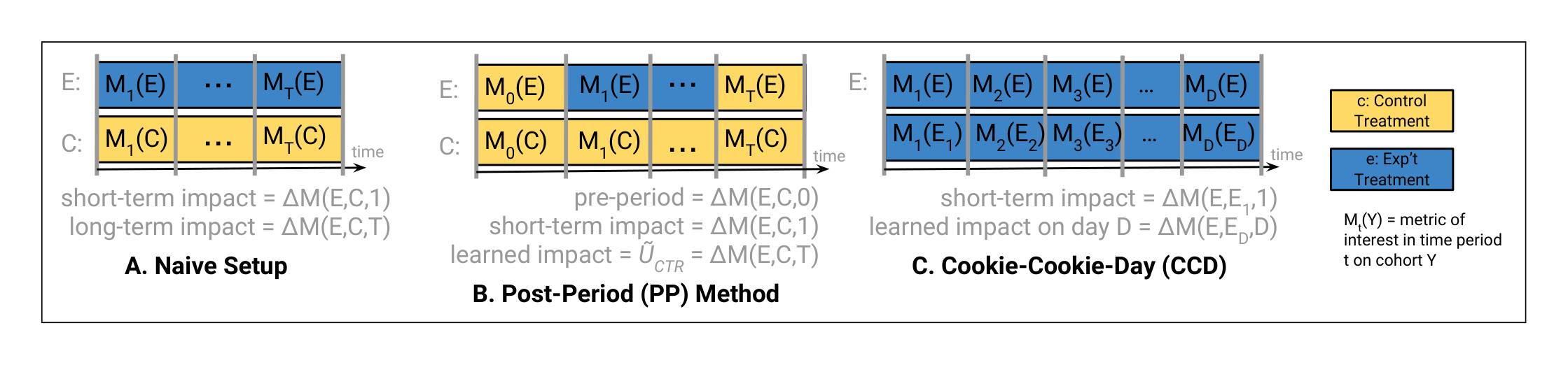
We call the set of randomized cookies that we follow over a period of time a cohort, which we denote with capital letters, such as $E$ for experiment and $C$ for control. The treatment that a cohort receives is denoted in lower case letters, such as $e$ for the experimental treatment and $c$ for the control treatment; a cohort could be exposed to different treatments at different times, e.g. $E$ might be in treatment $e$ from time $0$ to $T$ and then in treatment $c$.

We use relative changes throughout when comparing a metric $M$ in the experiment and control cohorts and define

$ \Delta M = \Delta M(E, C) = \frac{M(E) - M(C)}{M(C)}\tag{1} $

If a measurement is taken at a specific time $t$ we will sometimes make this explicit by writing $\Delta M(E, C, t)$. Note that all measurements made in this paper are aggregate measurements over a cohort and not on an individual user or cookie. Even when we measure user learning or user satisfaction, those measurements are done over the entire cohort.

An A/A test, or uniformity trial, is an experiment where instead of comparing an experimental treatment to a control, two cohorts are exposed to the exact same treatment in order to compare them or their behavior.

User learning was first proposed as Thorndike’s Law of Effect [19] and roughly states that positive outcomes reinforce the behavior that caused them and negative outcomes diminish the behavior that caused them. Modeling user learning with statistical models dates back to the 1950’s [4][5]. Studies of online behavior associated with user learning have primarily focused on novelty or primacy effects (users being presented with something new and either wanting to explore or needing time to adjust) or change aversion (users simply not liking change).

User learning is rarely studied at scale on large populations, with the exception of [14] that cautions against optimism in online experimentation when seeing novelty / primacy effects by claiming that they rarely, if ever, result in the outcome changing directionality.[^1] Kohavi et al. also note that experiments can result in carryover effects, where the treatment from an experiment on a cohort can impact the results from a follow-on experiment on the same cohort. We have independently observed such carryover effects in our systems and our methodology (Section 3) leverages them to study user learning at scale.

In this paper, we focus on a specific user learning effect: ads blindness and sightedness, which is when users change how likely they are to click on or interact with ads based on their prior experience with ads. Ads blindness and sightedness have been discussed since banner ads appeared on the web in the late 1990s. In [2], it was shown that users ignore text embedded in rectangular web banners, with location as a primary trigger. Subsequently, increased use of

[^1]: This is at odds with results we describe in Section 5.

animation was meant to draw user’s attention to ads and increase user’s rate of ad recognition [1]. A more recent study showed that text ads blindness also occurs, with users skipping sections that were clearly text ads (although sometimes returning later)[16].

All references describe small qualitative studies. Our work, to our knowledge, is the first to quantify, at scale, over millions of users and months of elapsed time, the effect of both ads blindness and sightedness, and apply those results to a large running system, namely Google search, which receives billions of searches per day from hundreds of millions of cookies in 200+ countries across multiple platforms (mobile, tablet, desktop, etc.).

Short-term impact is the measured difference between an experiment and control during the experiment period, typically days or weeks. The long-term impact is what would happen if the experiment launched and users received the experiment treatment in perpetuity – in other words, it is the impact in the limit $t \to \infty$. In the context of ads, differences between short- and long-term impact can mainly be attributed to user learning and advertiser response. Here, we focus on measuring and estimating the impact from user learning (the learned impact), specifically ads blindness and sightedness. We then approximate the long-term impact as the combination of the short-term and the learned impact.

Long-term revenue is a sensible OEC with an obvious focus on the long-term health of a business. Note that we can decompose revenue into component metrics as follows:

$ \text{Revenue} = \text{Users} \cdot \frac{\text{Tasks}}{\text{User}} \cdot \frac{\text{Queries}}{\text{Task}} \cdot \frac{\text{Ads}}{\text{Query}} \cdot \frac{\text{Clicks}}{\text{Ad}} \cdot \frac{\text{Cost}}{\text{Click}}\tag{2} $

This decomposition is useful, since it shows us that revenue, measured in the long-term, reflects user satisfaction since users could be:

• So unhappy that users abandon the product altogether (decreased number of users, term 1)
• Unhappy enough to decrease their usage of the product (fewer tasks per user, term 2)
• Sufficiently unhappy that they decrease how often they click on the ads (term 5), as well as which ads they click on (term 6)

The short-term interpretation of (2) suggests that increasing the ad load, i.e., the number of ads per query (term 4), would also increase revenue. One of our main results is that such gains may not persist in the long-term! To see this, first note that in an ad system that aims to show the highest quality ads to users, an increase in ad load usually leads to a decrease in the click-through rate (CTR = Clicks/Ad, term 5), even in the short-term. User learning may cause additional decreases in terms 1, 2, and 5 that may more than offset the increase in ad load, leading to reduced revenue in the long-term. In other words, increasing the ad load may increase short-term revenue but decrease long-term revenue since decreased user satisfaction causes ads blindness.

For Google search ads experiments, we have not measured a statistically significant learned effect on terms 1 and 2.[^2] Thus, we focus primarily on CTR, i.e., Clicks/Ad.

This discussion motivates the following definition. Consider any system change (‘treatment’) we may want to launch. We call the relative change in CTR due to user learning caused by launching the treatment Learned CTR, and we denote it by $U_{CTR}$. Some remarks:

• This definition does not give $U_{CTR}$ in a computable form. Rather, we imagine the change compared to a counterfactual setting, where no user learning occurs. We explain some of the reasons why $U_{CTR}$ cannot be measured directly in Section 3.3.
• We develop experimental methodology that enables us to measure approximations $\tilde{U}{CTR}$ of $U{CTR}$, e.g., as a percentage change in CTR in an experiment-control setting. We work with relative rather than absolute differences in order to control for the impact of seasonality as well as any system changes that launch during our experiment period.
• It may take months after a launch for the full effect $U_{CTR}$ to develop. We estimate the time it takes for user learning to occur in Section 3.2.1.
• $U_{CTR}$ tells us how users’ inherent propensity to click on ads (measured at a population-level) changes due to the treatment. Guided by Thorndike’s Law of Effect, we therefore consider $U_{CTR}$ a user-centric quality metric (users’ response to the treatment reflects their experience). Positive $U_{CTR}$ corresponds to ads sightedness, and negative $U_{CTR}$ to ads blindness.

In addition to describing how to estimate $U_{CTR}$ robustly, we create models that predict $U_{CTR}$ from short-term metrics so that we can predict long-term revenue as our OEC.

3. MEASURING USER LEARNING

Section Summary: To measure how users learn to ignore or notice ads—known as ads blindness and sightedness—researchers developed new experiment designs that focus on isolating learning effects from other influences. The main approach uses a post-period method, where experimental and control groups receive the same treatment after an initial test phase, allowing differences in user behavior during this follow-up to reveal learning without interference from external factors like seasonality. However, this technique can underestimate real-world learning due to issues like users unlearning habits over time, cookie changes, and the need for larger sample sizes to ensure reliable results.

Our first goal was to directly measure ads blindness and sightedness. This required new experiment designs and several months to run the experiments. The methodology described in this section is generally applicable for measuring user learning effects, but here we focus on measuring ads blindness and sightedness. We first describe the experimental designs and then lay out our basic ads blindness results. Finally, we discuss why our methodology understates the user learning effects in actual launches.

[^2]: We suspect the lack of effect is due to our focus on quality and user experience. Experiments on other sites indicate that there can indeed be user learning affecting overall site usage.

3.1 Experiment Design & Methodology

For the experiment methodology, we start with a naive setup before describing two methods, the Post-Period (PP) and the Cookie-Cookie-Day (CCD), that we developed.

3.1.1 Naive Setup

The obvious experiment design is to consider two cookie cohorts, $E$ and $C$, where $E$ receives some experimental treatment $e$ and $C$ receives a control treatment $c$, and track their metrics over time. The difference in metrics between $E$ and $C$ at the beginning of the experiment, $t = 1$, is the short-term impact of $e$, and the difference in metrics between $E$ and $C$ at the end of the experiment, $t = T$, is the long-term impact, including user learning (see Figure 1A). The experiment period will need to last for however long it takes for users to learn, which can be weeks, months, or more.

Unfortunately, even though time is taken to allow for users to learn, this naive setup does not yield reliable user learning measurements. The measured long-term effect at the end of the experiment period may change for many reasons unrelated to user learning: system effects, seasonality, interactions with subsequent launches, etc. Disentangling these effects to measure long-term learning within cohort $E$ over time is, in our experience, very difficult if not impossible.

3.1.2 Post-Period Learning Measurements (PP)

The key insight, in part stemming from observing carryover effects from prior experiments, is that to measure user learning, we need to compare the two cohorts, $E$ and $C$, while they receive the same treatment.

To achieve this, we sandwich the treatment period between two A/A test periods: a pre-period, where we ensure that there are no statistically significant differences between the cohorts when the study starts[^3], and a post-period (PP), where any behavioral differences due to user learning are measured. For the purposes of quantifying user learning, the behavior of $E$ while receiving treatment $e$ is not of interest – only the post-period measurement matters (see Figure 1B). Since $E$ and $C$ receive the same treatment in the post-period, differences between the metrics of the two cohorts in the PP can be ascribed to user behavior changes, i.e., to learning that occurred during the treatment period.

[^3]: Running a pre-period is good practice for all experiments and not just for measuring user learning.

In this way, we obtain PP user learning measurements $\tilde{U}_{CTR}^{PP} = \Delta CTR(E, C, T)$. We give examples in Section 3.2.1. Post-periods have proven to give reliable and reproducible user learning measurements at Google. Nevertheless, there are some caveats and limitations we want to point out.

Ensuring valid measurements. In practice, it may happen that despite receiving the same treatment, $E$ and $C$ do not experience identical serving in the PP due to personalization or other long-term features.[^4] In order to ensure a valid learning measurement, one needs to confirm that metrics that should be unaffected by user behavior changes, such as ads per query or the average predicted ad CTR, are consistent across $E$ and $C$.

[^4]: The problem is typically that the treatments $c$ and $e$ change the distribution of cookie-level long-term features in $C$ and $E$. These differences may cause $C$ and $E$ to receive systematically different serving even under the same treatment $c$. Examples of such long-term features are remarketing lists or mute-this-ad data. Care should be taken to minimize such feedback if the goal is to measure user learning.

Also note that the measurement environment $c$ of the post-period may affect the magnitude or nature of the learning effects observed. As a basic example, if $e$ adds a great new UI feature that users learn to interact with more over time, we will not be able to observe this in a post-period serving $c$ where the feature is absent.

Unlearning. Since both $E$ and $C$ receive the same treatment in the PP, their behavior will become more similar over time, that is, unlearning will occur. Thus, our measurement would ideally be taken in a brief period right at the beginning of the PP. However, for a given experiment size, we can increase statistical power by taking the measurement over a longer period of time. The price to pay is measurement bias introduced by unlearning. This bias can be corrected based on (un)learning rates, see Section 3.2.1.

Cookie churn. Cookie churn occurs when users reset or clear their cookies, leading to random movement between experiments. Including new cookies in the experiment and control dilutes the user learning effect measured. This issue can be addressed by restricting the measurement to cookies that were created before the start of the experiment. Note that restricting to old cookies may introduce bias.

Experiment sizing. To ensure that our studies are adequately powered, we use the best practices enshrined in the experiment sizing tool described in [18]. As noted there, using cookies as the experimental unit requires larger sizes than experiments that divert on individual query events, since one has to account for the non-independence of queries coming from the same cookies over time.

Unlearning and cookie churn also affect the statistical power of the experiments. We studied the cookie age distribution to allow us to estimate the number of cookies that would be lost from the post-period comparison because of cookie churn and to scale up the size of $E$ and $C$ as needed.

Intermediate measurements and lagged-starts. One serious disadvantage of the PP method is that the learning measurement is taken after the treatment period, i.e., the measurement requires ending the treatment period. No preliminary measurements of learning are obtained along the way. This can be problematic since the required length of the treatment period can depend on the treatment studied and may not be known in advance.[^5]

[^5]: In Section 3.2.1, we will describe an approach to determine appropriate treatment period durations, but such prior information is not always available.[^5]

One way of obtaining a preliminary measurement is by adding an extra lagged-start cohort $E_1$. We keep $E_1$ in the control treatment $c$ while $E$ already receives the experimental treatment $e$ until we want to take a learning measurement, say at time $T_1$. At $T_1$ we switch $E_1$ from $c$ to $e$. We can now obtain a user learning measurement $\tilde{U}_{CTR}^{LS} = \Delta CTR(E, E_1, T_1)$ by comparing $E$, which was exposed to $e$, to $E_1$, which was previously exposed to $c$.

The important point here is that, as in the PP method, the learning measurement is taken when the two cohorts receive the same treatment (here the experiment treatment $e$). Note that taking this lagged-start measurement does not require ending the treatment period of $E$. We can take several lagged-start measurements during the treatment period, but each additional measurement will require its own lagged-start cohort $E_1$, $E_2$, etc.

3.1.3 The Cookie–Cookie-Day Method (CCD)

This method is derived from the idea of continuously taking lagged-start measurements in order to track user learning while it happens. In fact, we construct daily measurements by essentially using a different lagged-start cohort for every treatment day.

Cookie-day experiments. We obtain such cohorts by using an experimental unit that is a combination of the cookie and the date, so that cookies are re-randomized into experiments daily. Experiments based on such experimental units are called cookie-day experiments.

In practice, we start with a large pool of cookies, and on each day we randomly assign a fraction of these cookies to the experiment. If the cookie pool is sufficiently large, each cookie will only be assigned to the experiment on very few days so that, in essence, we treat a different cookie cohort on any given day. In particular, each cookie will not receive consistent enough exposure to the experiment treatment to accumulate any learned effect.

The Cookie–Cookie-Day comparison. In the Cookie–Cookie-Day (CCD) method, we compare cookie and cookieday experiments receiving the same treatment $e$.[^6] In the cookie experiment, cohort $E$ receives the treatment $e$ every day and experiences user learning. In parallel, we run a cookie-day experiment where a different cohort $E_d$ is exposed to $e$ on any given day $d$. On all other days, $E_d$ receives the control treatment $c$.[^7] As in the lagged-start setting, user learning can be measured on day $d$ by comparing the metrics of $E$ to $E_d$: this is the CCD comparison (see Figure 1C).

[^6]: Within a single layer, for those familiar with the Overlapping Experiments framework [18].

[^7]: In our actual implementation, in order to manage experiment traffic more efficiently, the cookie-day cohorts $E_d$ may not receive $c$ on every day $d' \neq d$. Rather, they see a mix of treatments that, on average, is very similar to $c$ and so the learning effects are approximately the same. We usually also run a cookie-day version of the control (on day $d$ cohort $C_d$ will get the the control treatment); by comparing $C_d$ to a control cookie cohort $C$ we can check that cookies in the cookie-day space do not accumulate a learned effect.

The main advantage of CCD is that learning can be tracked continuously while it is happening: the daily measurements $\tilde{U}_{CTR}^{CCD}(d) = \Delta CTR(E, E_d, d)$ fit together to yield a time series describing learning over time. This can help inform the length of the study: if learning is still going strong, one might want to extend the experiments, whereas if no effect

is visible after two months, chances may be slim to observe anything even when running longer. The time series of learning measurement can also be useful in estimating learning rates and detecting issues in the experiment set-up.

Another upside of CCD is that learning can be measured over a longer period of time than in the PP method since unlearning is not a concern. Such extended measurement periods can significantly reduce noise. The main disadvantages of CCD are the increased infrastructure complexity and the need for a large cookie pool that provides traffic for the cookie-day experiment.

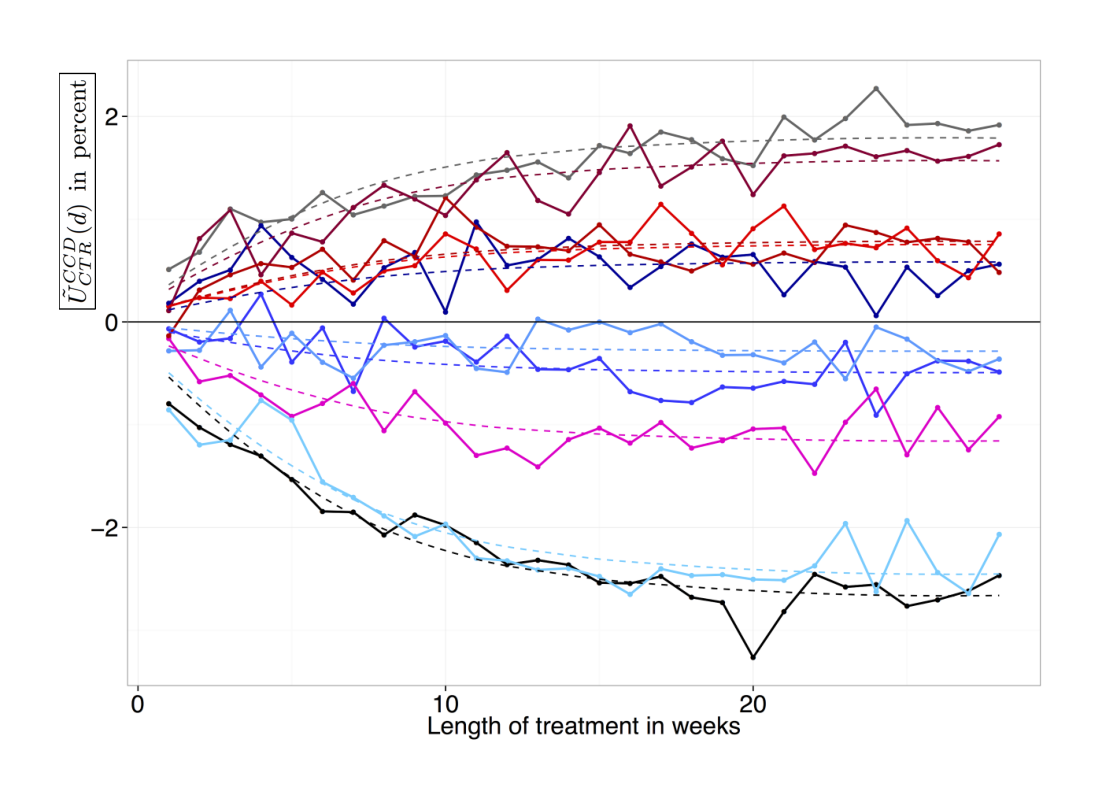
To illustrate the efficacy of the CCD method, Figure 2 shows a time series of learned changes in CTR, i.e. $\tilde{U}_{CTR}^{CCD}(d)$, for a grid of ten settings of a system parameter over six months, along with exponential trends fit to the data.

As a best practice, we recommend combining both methods: run a CCD setup and also take a PP measurement on the cookie cohort $E$ after the treatment period is over. We have generally found the measurements $\tilde{U}{CTR}^{PP}$, $\tilde{U}{CTR}^{LS}$, and $\tilde{U}_{CTR}^{CCD}$ to produce consistent results.

3.2 Ads Blindness Studies

Since 2007, we have run hundreds of experiments to quantify ads blindness and sightedness. The main output from this work is an OEC that depends only on short-term metrics but predicts the long-term impact (see Section 4). Using this OEC to make launch decisions has improved the ads we show to users. Here we summarize some of the major steps in collecting the data necessary to build these models.

3.2.1 Initial Experiments

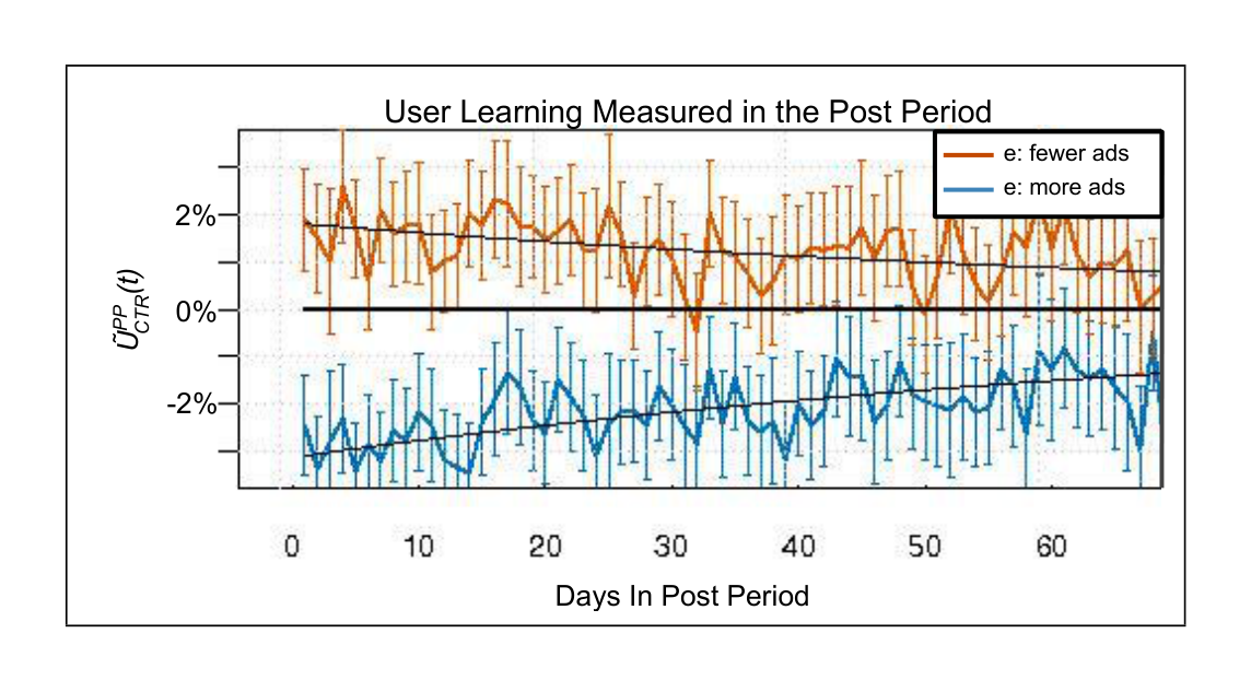
The goal of our initial user learning experiments was to explore the magnitude of treatments needed to induce measurable learning effects and to see how long learning takes. These experiments were run before we developed the CCD method, so we used a combination of the PP and lagged-start methods to obtain user learning measurements.

We used two different experimental treatments. One treatment increased the ad load, and the other reduced it. Since we are always trying to show the best ads to our users, any additional ads will have slightly lower quality so that the average quality of ads decreases as the ad load increases. In particular, these treatments conflate ads quality and ad load, something we tried to disentangle in later experiments.

Ads blindness can be measured. This basic result can be seen in Figure 3, which shows the relative change in CTR of the cohorts exposed to the two treatments relative to the control cohort in the post-period. Showing fewer but higher quality ads resulted in ads sightedness (positive $\tilde{U}{CTR}^{PP}$); showing more but lower quality ads resulted in ads blindness (negative $\tilde{U}{CTR}^{PP}$).

User learning takes a long time. A more subtle goal of the initial experiments was to quantify the time period needed for user learning to occur, i.e., determining when the user learning impact on CTR (the change in users’ click propensity) would plateau. We used repeated lagged-start measurements to verify that the learned effects still increased, even after many weeks of treatment. In other words, user learning takes a long time to converge.

A simple learning model. As mentioned in the discussion in Section 3.1.2, PP measurements are, in practice, taken over an extended period of time. This yields a time series $\tilde{U}_{CTR}^{PP}(t) = \Delta CTR(E, C, t)$ for $t \ge T$ as in Figure 3.

In order to obtain a quantitative result on the pace of user learning, we fit a simple exponential curve to model $\tilde{U}_{CTR}^{PP}(t)$ (effectively modeling unlearning rather than learning)[^8]:

$ \tilde{U}_{CTR}^{PP}(t) = \alpha \cdot e^{-\beta \cdot (t-T)} \quad \text{for } t \ge T\tag{3} $

[^8]: We also used learning data from lagged-start measurements to fit these models, but do not discuss this here for simplicity.

Here $\alpha$ estimates the magnitude of learning at the beginning of the post-period $T$, and $\beta$ is the (un)learning rate. We assumed a constant learning rate $\beta$ across different treatments but $\alpha$ was assumed to be treatment dependent (and is the focus of the modeling discussed in Section 4).

The half-life of learning $\ln(2)/\beta$ was approximately 60 days (see Figure 3), or $\beta \approx 0.012$ per day. This learning rate was later validated in a CCD study, where we modeled

$ \tilde{U}_{CTR}^{CCD}(t) = \alpha' \cdot (1 - e^{-\beta \cdot t}) \quad \text{for } t \ge 0\tag{4} $

with $\alpha'$ estimating the magnitude of learning we would measure in a very long study ($t \to \infty$).[^9]

In this section, we have considered learning rates as a function of time. We explored alternatives, such as considering them as a function of the number of user interactions (e.g., searches issued or ads viewed). However, we use time for convenience as it allows us to aggregate all users’ activities across a day and do all analysis in this aggregated space.

Standard ads blindness studies. Based on the learning rate estimate $\beta \approx 0.012$, we now typically run long-term desktop experiments for 90 days, which gives a reasonable trade-off between study run-times and captured learning effects. According to (4), the learning observed after 90 days is approximately $1 - e^{-0.012 \cdot 90} = 65%$ of the learning effect we would see in a very long experiment.[^10]

In the following sections, we denote by $\tilde{U}_{CTR}$ ads blindness or sightedness measurements taken in ‘standard studies’ lasting about 3 months. These may be PP, lagged-start, or CCD measurements.

Note that we can also apply the model (3) to understand the bias in PP measurements due to unlearning. Assume we take the measurement in the first two weeks of the post-period and that each day contains the same amount of data. Then unlearning reduces the effect observed over the 14 days of the measurement to $\frac{1}{14} \sum_{j=1}^{14} \exp(-0.012 \cdot j) = 92%$.

Hence $\tilde{U}_{CTR}$ measured in the first 14 days of a post-period in a standard learning study is $65% \cdot 92% \approx 60%$ of the effect observed in a very long running study (on desktop).

[^9]: The exponential trends for the mobile study in Figure 2 were obtained in the same way.

[^10]: The learning rate may depend on the treatment, e.g., the triggering rate of a feature, but we have found these results to hold for a reasonable variety of system changes.

3.2.2 The Dropping Study

While the initial study verified the existence and quantified the rate of user learning for ads blindness and sightedness, we were dissatisfied with the conflation of ads quality and ad load. To address this issue, we devised our next set of experiments, in 2010, to explicitly control the quality of the shown ads. Specifically, we divided the ads into tiers by their ads quality scores. We then ran PP method experiments with the following treatments:

• $e$: Increase the ad load, with the same conflation of ads quality and ad load as above.
• $e_1, \dots, e_n$: We want these treatments to have the same ad load as $c$ but different ads quality. We achieve this through a series of system manipulations. We first increase the ad load and then reduce it back to the level of $c$ by dropping ads from a specific quality tier $i = 1, \dots, n$. The ads quality of $e_i$ decreases as $i$ increases.
• $e'$: Same as for $e_i$, in that we increase the ad load to the same level as $e$, but we then drop ads uniformly across all quality tiers to achieve the same ad load as $c$ but with an average ads quality comparable to $e$.

Bringing the corresponding cookie cohorts $E, E_1, \dots, E_n, E'$ to post-period, we could determine if quantity was the driver (in which case $\tilde{U}{CTR}(E, C)$ would be more negative than $\tilde{U}{CTR}(E', C)$), or if quality was the driver (the effect of $E_1$, where we dropped the highest quality ads, would be more negative than that of $E_2$, which would be more than $E_3$, etc., and $E'$ would be somewhere in the middle).

Our results showed that cohorts that experienced higher ad quality than the control during the treatment had positive $\tilde{U}{CTR}^{PP}$ (ads sightedness) and that cohorts exposed to lower quality had negative $\tilde{U}{CTR}^{PP}$ (ads blindness). We did not measure a significant learning effect in the post-period comparison of $E$ and $E'$, $\tilde{U}_{CTR}(E', E)$. Therefore we concluded that ads quality is the main driver of user learning.

Note, however, that in practice ad load does matter since it is correlated with ads quality in systems that strive to show the best possible ads to users.

3.2.3 Subsequent Experiments

The initial experiments and the dropping study provided our first models for understanding ads blindness and sightedness: the rate of learning, the magnitude of the long-term effects relative to the short-term impact, and the main drivers behind the effect. Over the last eight years, we have run hundreds of long-term experiments to increase our understanding, especially regarding the drivers of user learning. We designed learning studies to address specific questions, such as: Does the type of task matter? How does ad relevance differ from landing page quality in driving the magnitude of the effect? How do UI changes impact user learning?

These studies allowed us to improve the algorithms that select the best ads to show to users. In Section 4, we use data from these experiments to predict the magnitude of ads blindness or sightedness from short-term metrics.

3.3 Underestimation of Results

In this section, we discuss why the PP and CCD methods both yield systematic underestimates of true long-term user learning effect $U_{CTR}$. By this, we mean that if we launched a treatment to all users, the user learning effect would be larger than the effect $\tilde{U}_{CTR}$ we measure in our experiments. How severely our measurements underestimate user learning is difficult to estimate since learning is not just a function of time, but also a function of the number, frequency, and consistency of exposure to the treatment.

Number and frequency of exposure. Intensity of exposure to the treatment affects the learning rate. For example, the $\beta$ derived in Section 3.2.1 depends on how often users search on Google and on how often ads show on their queries. Measuring learning for features that show on more queries than ads can be done using shorter treatment periods (for changes that impact every search results page, we estimate that half the learning has happened after 14-21 days). Conversely, learning on features that show less often than ads may take a lot longer, to the point of being impossible to measure.

Even for ad-centric studies, the learning rates may vary. For example, learning induced by an ad format with low triggering rate or a subtle UI change might take a long time to materialize. Due to this uncertainty, using the CCD methodology to measure learning in real-time is helpful.

Treatment inconsistency. The bigger issue is that cookies are a poor proxy for users. A cookie is simply an anonymous id attached to a browser and a device. Users can clear their cookies whenever they want, and they frequently use multiple devices and multiple browsers. Thus, any learning measured from a cookie-based experiment is diluted since a user is likely seeing non-experiment treatments on other browsers: there is less consistency in an experiment than there is when the change is launched. Using a signed-in id may seem to mitigate this issue, but users can have multiple sign-ins and many searches are conducted while signed-out.

Accounting for underestimation. In the discussion of OECs in Section 4.4 below, we want to be explicit about the distinction between user learning when a treatment is launched ($U_{CTR}$) and the potentially weaker learning effect $\tilde{U}_{CTR}$ we observe in standard PP or CCD measurements. To this end, we introduce a ‘fudge factor’ $Q$ defined by

$ U_{CTR} = Q \cdot \tilde{U}_{CTR}.\tag{5} $

Since the user learning measurement methods we presented here underestimate learning, we have $Q \ge 1$. Both number and frequency of exposures and consistency issues contribute to $Q$. As a result, $Q$ depends on our decision to run long-term experiments for 90 days and, since treatment consistency differs by platform, it also differs by device type.

How large is $Q$? Generally, this is a difficult question to answer. The exponential learning model from Section 3.2.1 implies that in a 90-day study we would only measure about 65% of the long-term effect simply due to the limited study duration, not even accounting for lack of treatment consistency. Hence we have $Q \ge 1/0.65 = 1.54$ for a standard learning measurement in a desktop study. In practice, we often use values of $Q$ between 2 and 3 for desktop and laptop devices in order to also compensate for treatment inconsistency. This range, though only a rough estimate, has been supported by a study considering learning effects of cohorts of cookies with very high treatment exposure.

Our exponential models for mobile (not discussed here, but observable in Figure 2) suggest that learning is faster on smartphones, and we also believe the consistency issue to be less severe. As a result, we think $Q$ is closer to 1 for mobile and have, in fact, often assumed the minimal possible value $Q = 1$ in this case.

Other sources of user behavior changes. In this section, we have been concerned with underestimates of learning arising from low treatment dose and an imperfect relationship between cookies and users. However, there are factors affecting long-term user behavior on Google search that cannot be captured in experiments at all. For example, perception of poor ads quality may be amplified by word-ofmouth or negative press reports.

4. PREDICTING ADS BLINDNESS

Section Summary: Instead of waiting months for long-term experiments to measure ads blindness, where users become less responsive to ads over time, researchers have developed macro-models to predict these effects using short-term data from standard A/B tests. These models, built from over 100 past experiments, forecast changes in user click behavior based on factors like ad load increases, which typically reduce clicks, or improvements in ad relevance and landing page quality, which boost engagement. The models are simple linear equations for easy interpretation and have shown reliable accuracy across various ad system tweaks, such as algorithm changes.

Thus far, we have discussed how to measure user learning in long-term experiments. Now we tackle the issue of predicting the ads blindness or sightedness effect rather than waiting for months to measure it. The simple exponential models we fit in Section 3.2.1 gave us the time that we would have to wait, but not the magnitude of the effects. In order to apply ads blindness to day-to-day decisions, we need to be able to take the short-term measurements and use them to predict the magnitude of the long-term effect.

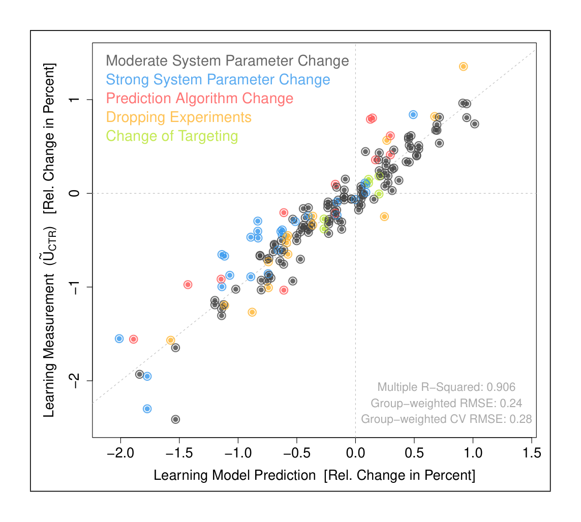
We now present models doing precisely this. We call them macro-models since they make predictions at the population level. To create these models, we use the results from more than 100 long-term ads blindness experiments, collected over several years, that test a range of changes, from new prediction algorithms to optimizing system parameters to changing the keyword matching algorithms and more.

Since all data considered here is from PP or CCD studies, we use $\tilde{U}_{CTR}$ as the user learning metric our models predict (response). The model covariates (predictors) are short-term treatment metrics, i.e. the instantaneous metric changes observed when the treatment is applied in a short-term experiment. In the notation of Figure 1, covariates are defined by $\Delta M = \Delta M(E, C, 1)$, for suitable metrics $M$.

Thus, all metrics on the right-hand side of the models below are short-term quantities that are easy to measure in a standard A/B experiment setup, whereas the left-hand side is the long-term user behavior change we are predicting. All equations below are dimensionless as all metrics are relative changes between experiment and control.

4.1 Ad-Load-based Models

The change in ad load is a good linear predictor for the resulting change in user clickiness when the treatment is just a simple ad load change, as in the initial experiments described in Section 3.2.1 or similar follow-up studies. This is expressed succinctly by the macro model

$ \tilde{U}_{CTR} \approx -k \cdot \Delta \text{AdLoad}\tag{6} $

with $k > 0$. This model states that showing more ads results in ads blindness, i.e., a decrease in users’ propensity to click on ads. We have observed the relationship (6) for ad load changes of moderate magnitude in various settings (different sites or device types) but with varying values of $k$.

However, (6) only applies to simple ad load changes where ad load and ads quality are directly (negatively) correlated, as in our original experiments. While the applicability of (6) is thus restricted to a small set of treatments, it has nevertheless proven useful (e.g., the mobile example in Section 5).

4.2 Quality-based Models

As discovered in the experiments described in Section 3.2.2, the main driver of ads blindness is the ads quality rather

than the ad load. Given those findings, our subsequent and more generally applicable macro-models used ads qualitybased metrics rather than ad load-based metrics.

Many of these models are of the form

$ \tilde{U}_{CTR} \approx k_1 \cdot \Delta \text{AdRelevance} + k_2 \cdot \Delta \text{LandingPageQuality}\tag{7} $

with $k_1, k_2 > 0$. The interpretation of (7) is intuitive: better AdRelevance and/or LandingPageQuality increase user engagement with ads. While the form of (7) has been consistent over the last few years, our definitions of the AdRelevance and LandingPageQuality metrics used in the model have evolved over time. The simplest example of an AdRelevance metric is CTR. LandingPageQuality metrics are generally more complex and consider the actual content and experience of the landing site [8].

In our experience, good macro-models require both an ad relevance and landing page quality term: we have not found satisfactory single variable blindness models. In particular, we have found that AdRelevance alone is insufficient to characterize ads quality and that user satisfaction after a click is also very important. This makes sense: if an ad looked good but the user had a horrible experience after the click, the user will remember the bad experience on the landing page and the propensity of future ad clicks decreases.

We have found that ads-quality-based models such as (7) capture ads blindness and sightedness reasonably well for a wide variety of non-UI manipulations such as ad load, ranking function, and prediction algorithm changes. This can be seen in Figure 4, which plots predictions from our current desktop macro-model against the actual measurements $\tilde{U}_{CTR}$ for the 170 observations used to fit the model. We have a similar model for the mobile interface of Google search.

4.3 Remarks on Methodology

The macro-models given above are simple linear models, with weights according to measurement precision. The main reason to stick to such simple models is interpretability. We considered using larger predictor sets and regularization, but the gains in prediction accuracy were rather modest and not worth giving up models with well-understood semantics. Naturally, such simple linear models can only cover a limited range of serving configurations, but we have found their validity to be pretty broad in practice.

Our models were evaluated using cross-validation, with cross-validation folds being manually chosen groups of similar experiments. This was done to avoid overfitting, which is a huge concern given the small sample size.

Another requirement imposed on more general models was that prediction accuracy on simple experiments should not be worse than that of very plain models, such as (6), known to work well in certain cases. The most important criterion for our models is, of course, their prediction accuracy on new data, and we continually validate our models by comparing predictions against measurements in new studies.

The models given here are specific to Google search. Nevertheless, we expect the fundamental principle to apply in other contexts: quality drives user interaction, and suitable user experience signals can be used to predict changes in user engagement (e.g., click-through or page visit rates).

4.4 Long-term Impact and OECs

4.4.1 Approximations of Learned RPM

The change of user engagement with ads, as captured by the quality metric $U_{CTR}$, alters the revenue impact of a system change in the weeks and months after its launch. Analogous to the definition of $U_{CTR}$, we define $U_{RPM}$ to be the relative change in RPM (revenue per 1000 queries) due to user learning caused by the launched treatment.[^11]

If a change in users’ propensity to click on ads is the only user learning effect we observe, which is often the case on Google search, then

$ U_{RPM} \approx U_{CTR} .\tag{8} $

This can be seen from the revenue decomposition (2). For example, if CTR decreases by 1%, then so does revenue. The right-hand side of (8) can be expressed as $Q \cdot \tilde{U}_{CTR}$ via (5), and computed using the models from Sections 4.1/4.2.

When revenue is generated from several segments of ads, one needs to use

$ U_{RPM} \approx Q \cdot \sum_i w_i \cdot \tilde{U}_{CTR, i}\tag{9} $

where we measure $\tilde{U}_{CTR, i}$ separately for different segments $i$, and $w_i$ gives the revenue fraction in the segment. The different segments reflect differences in Learned CTR or major differences in click costs. Cases where this segmentation is particularly important include ad location on the page and geography, where the bids can differ, either due to standards of living, currency exchange, or the number of advertisers.

These approximations of $U_{RPM}$ are needed since measuring $U_{RPM}$ directly in a long-term study is often impossible due to statistical noise.

4.4.2 Longterm RPM

We often combine the instantaneous revenue change of a treatment, $\Delta RPM = \Delta RPM(E, C, 1)$, and the RPM change due to user learning $U_{RPM}$ into a single long-term metric

$ LTRPM = \Delta RPM + U_{RPM} .\tag{10} $

[^11]: We can use RPM instead of revenue since we have not measured changes in the first three terms of (2).

$LTRPM$ aims to approximate the long-term revenue impact of a launch.[^12] The interpretation of (10) is straightforward: the expected long-term RPM effect is given by the observed instantaneous revenue change plus a correction term that expresses how user behavior changes will alter RPM post-launch. Note that (10) defines an OEC that focuses on long-term business health, given that, for Google search, we did not see changes in the first 3 terms of (2) in Section 2.

Using the approximation (8), we obtain:

$ LTRPM = \Delta RPM + Q \cdot \tilde{U}_{CTR}\tag{11} $

Recall that our macro-models allow us to express $\tilde{U}_{CTR}$ in terms of short-term metrics. Thus (11), together with our macro-models, solves the problem of defining an OEC with emphasis on the long-term that can be readily computed from short-term metric measurements, which was our original goal.[^13] The two summands in the OEC (11) express that long-term business health depends both on creating revenue and providing a good user experience. An obvious aspect missing in (11) is advertiser value, which we currently verify through separate metrics. Building an OEC that reflects the launch impact on Google, users, and advertisers is an active area of research at Google.

5. APPLICATIONS OF ADS BLINDNESS

Section Summary: Research on ads blindness has directly improved user satisfaction and decision-making for Google search ads by helping predict long-term effects of changes, rather than relying on short-term data. In one application, a 2011 update to the ad ranking system placed more emphasis on landing page quality, validated through studies that accounted for users' tendency to ignore ads over time. Another key example from 2013 involved reducing mobile ad loads by 50% after experiments revealed that adding more ads boosted short-term revenue but led to long-term declines due to user blindness, ultimately enhancing user experience while maintaining positive revenue impacts.

Ultimately, the success of our work is measured by whether we improved user satisfaction and affected decision-making for search ads on Google. The answer is unequivocally yes! Understanding ads blindness (Section 3) has changed the nature of the discussions around evaluating changes. We have used the models discussed in Section 4 to predict the long-term impact of experimental treatments to support or reject potential changes. Here are two specific examples.

Ranking function change. In October 2011, our ads blindness work drove a change in the quality score used in the auction ranking function that emphasizes the landing page experience more [10]. We ran numerous studies to

[^12]: The ‘long-term revenue impact of a launch’ is the relative difference in revenue (a sufficiently long time period after the launch), compared to the counterfactual scenario where the launch did not happen.

[^13]: For treatments where our macro-models do not work, we often fall back to measuring $\tilde{U}_{CTR}$ directly in a blindness study. This is cumbersome but sometimes necessary.

understand the long-term impact of the proposed (and ultimately launched) change as well as to validate our prior learnings. While we had taken the identified metrics from Section 4 into account for our OEC prior to this launch, this launch was when we really moved to using what we learned about ads blindness to impact per-query decisions.

Mobile ad load. In another example, our experiments were used to determine the appropriate ad load for searches on Google from mobile devices.

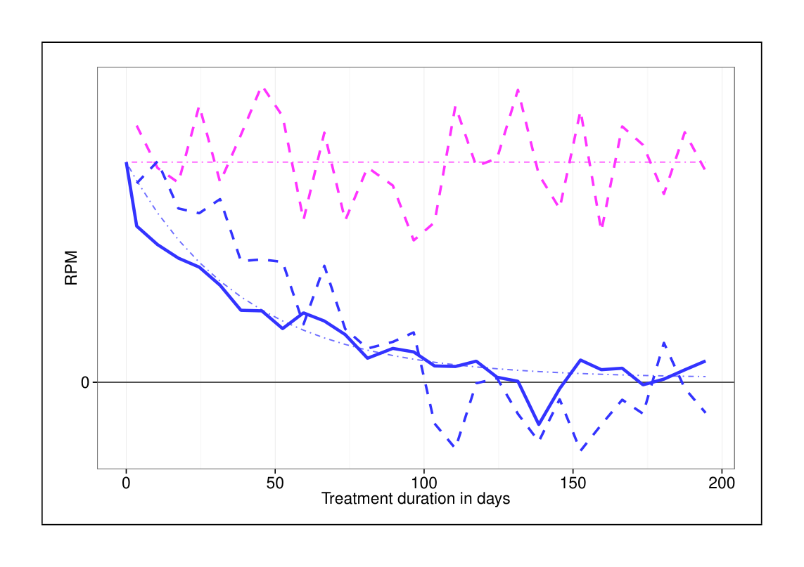
In 2013 we ran experiments that changed the ad load on mobile devices, similar to the experiments described in Section 3. Figure 5 shows results for an experiment that increased the ad load. The dashed lines give weekly RPM measurements for the cookie-day (pink, includes no user learning) and the cookie (blue, reflects learning) experiments of the study. The thinner horizontal pink line gives the cookieday average: this is the short-term RPM change $\Delta RPM$. The solid blue line gives $\Delta RPM + \tilde{U}_{CTR}(d)$, which approximates $LTRPM$ (with $Q = 1$) as $d$ gets large. It hugs a smooth curve based on a simple exponential learning model as described in Section 3.2.1. Since the blue curves settle near 0 as the study runs longer, the long-term revenue estimate $LTRPM$ for this treatment is essentially zero – in stark contrast to the significant short-term RPM gains – even under the idealized assumption of complete treatment consistency ($Q = 1$). In reality, the increased ads load is likely long-term negative at the state of the system during the study.

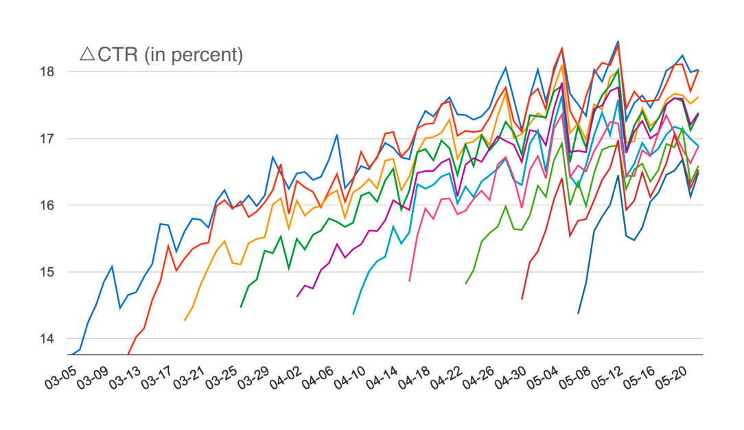
This and similar ads blindness studies led to a sequence of launches that decreased the search ad load on Google’s mobile traffic by 50%, resulting in dramatic gains in user experience metrics. We estimated that the positive user response would be so great that the long-term revenue change would be a net positive. One of these launches was rolled out over ten weeks to 10% cohorts of traffic per week. Figure 6 shows the relative change in CTR for different cohorts relative to a holdback. Each curve starts at one point, representing the instantaneous quality gains, and climbs higher post-launch due to user sightedness. Differences between the cohorts represent positive user learning, i.e., ads sightedness.

6. CONCLUSIONS & FUTURE WORK

Section Summary: This paper introduces methods to measure how users learn over time and to predict long-term effects from short-term data, applied to how people interact with online ads based on their quality. The research influenced key changes at Google, such as better metrics for ad performance, updates to the ad auction system prioritizing user experience, and a 50% cut in ads on mobile search pages. Looking ahead, the team plans to extend this approach to other websites and features like video platforms or shopping tools, while tackling challenges like varying site designs and developing finer predictions for single ad views.

In this paper, we have presented experimental methodology for quantifying long-term user learning and modeling methodology that uses the experimental results to identify which short-term metrics best predict the long-term userlearning impact.

We have applied these methodologies to a concrete use case, ads blindness and sightedness, and shown that users do in fact change their interaction rate with ads based on the quality of the ads they see and click on. These studies have been highly impactful:

• We created a frequently used OEC that accounts for both short-term and long-term impact.
• They were fundamental to a major conceptual change to our search ads auction that emphasizes landing page experience more.
• Launches that reduced the ad load on the Google search mobile interface by 50% were driven by our results.

Work beyond the scope of this paper includes the application of this methodology to sites other than Google search pages – both search pages on other sites as well as nonsearch-based interfaces (e.g., YouTube, display ads). One challenge is how to handle the increased heterogeneity of the sites in the modeling. That said, some initial results on other search sites with substantially higher ad load and lower quality are quite promising, with results even stronger than those discussed in Section 5, including impact to query volume and other terms in (2). We have communicated the results of these experiments to several partners, who have reduced their ad load and increased the quality, leading to positive long-term results for users and their business.

We have also applied this methodology to user learning beyond ads, specifically for experiments on bolding and labeling changes on the search results page, as well as other features such as Google Shopping.

We continue to work on better estimates for the correction factor $Q$. Also, our current models are based solely on (and applicable to) non-UI changes. The key challenge with integrating UI changes is that we have not identified metrics that appropriately capture the impact of UI changes on user experience and could serve as predictors in our model.

Finally, the models we describe in Section 4 predict a population-level learned ads blindness response that can be used at a macro-level, e.g., for launch decisions or validating quality metrics. We are working on “nano-models” that aim to predict the blindness cost of individual ad impressions, i.e., the future revenue loss (or gain) caused by showing an ad to the user. However, these models are substantially more difficult than the macro-models we have presented due to the sparse data available at the impression level and because this problem requires inference from observational data, lacking the clean randomization of an experiment-control setup.

Acknowledgments. Jean Steiner contributed greatly to the experiments and analysis described in Section 3.2.2. Ryan Giordano was a major contributor to ads blindness modeling and in particular the considerations described in Section 3.3. Marc Berndl and Ted Baltz designed and implemented many blindness experiments and drove the auction change launch described in Section 5 (Ted was also critical for the mobile changes), and with Rehan Khan and Bill Heavlin were instrumental in some of the initial framing of ads blindness. Chris Roat and Bartholomew Furrow contributed to the experiment and analysis implementation. Mark Russell worked on the study extending these methodologies to other search sites. An incomplete list of technical contributors includes Amir Najmi, Nick Chamandy, Xiaoyue Zhao, Omkar Muralidharan, Dan Liu, Jeff Klingner, Kathy Zhong, and Alex Blocker. This work was supported through the years (both by adopting the results in decision-making and by allowing us to run very expensive experiments) by Sridhar Ramaswamy, Nick Fox, Jonathan Alferness, Adam Juda, Mike Hochberg, and Vinod Marur. Adam Juda, Ben Smith and Tamara Munzner helped make this paper understandable to a wider audience. (Tamara was also critical in the original Overlapping Experiments publication.) Roberto Bayardo, Sugato Basu, Mukund Sundararajan, Jeff Dean, Greg Corrado, and Maya Gupta gave valuable feedback on preliminary versions of this paper.

7. REFERENCES

Section Summary: This section provides a bibliography of sources cited throughout the document, including academic papers, conference proceedings, and online articles. It covers topics like user blindness to web advertisements, psychological theories of learning, Google's guidelines on ad quality and landing pages, and methods for conducting trustworthy online experiments at companies like Amazon and Microsoft. The references span from historical works on animal intelligence in the late 1800s to recent publications in the 2010s, drawing from fields such as usability studies, data mining, and digital marketing.

[1] M. Bayles. Just how “Blind” Are We to Advertising Banners on the Web? In Usability News, 22 2000.

[2] J.P. Benway, D.M. Lane. Banner Blindness: Web Searchers Often Miss “Obvious” Links. www.ruf.rice.edu.

[3] A. Broder, M. Ciaramita, M. Fontoura, E. Gabrilovich, V. Josifovski, D. Metzler, V. Murdock, V. Plachouras. To Swing or not to Swing: Learning when (not) to Advertise. In CIKM 2008.

[4] R.R. Bush, F. Mosteller. A Mathematical Model for Simple Learning. In Psychological Review, 58 1951.

[5] W.K. Estes. Toward a Statistical Theory of Learning. In Pyschological Review, 57 1950.

[6] Google. AdWords Help: Check and understand Quality Score. support.google.com.

[7] Google. AdWords Help: Things you should know about Ads Quality. support.google.com.

[8] Google. AdWords Help: Understanding Landing Page Experience. support.google.com.

[9] G. Hotchkiss. More Ads = Better Ads = Better User Experience: Microsoft’s Success Formula? searchengineland.com.

[10] A. Juda. Ads quality improvements rolling out globally. adwords.blogspot.com.

[11] R. Kohavi, M. Round. Front Line Internet Analytics at Amazon.com. ai.stanford.edu.

[12] R. Kohavi, R. Henne, D. Sommerfield. Practical Guide to Controlled Experiments on the Web: Listen to Your Customers not to the HiPPO. In KDD 2007.

[13] R. Kohavi, T. Crook, R. Longbotham. Online Experimentation at Microsoft. In Third Workshop on Data Mining Case Studies 2009.

[14] R. Kohavi, A. Deng, B. Frasca, R. Longbotham, T. Walker, Y. Xu. Trustworthy Online Controlled Experiments: Five Puzzling Outcomes Explained. In KDD 2012.

[15] R. Kohavi, A. Deng, B. Frasca, T. Walker, Y. Xu, N. Pohlmann. Online Controlled Experiments at Large Scale. In KDD 2013.

[16] J.W. Owens, B.S. Chaparro, E.M. Palmer. Text Advertising Blindness: The New Banner Blindness? In Jounal of Usability Studies, May 2011.

[17] G. Sadler. Why Not Treat Marketing Like Sales? www.dnb.com.

[18] D. Tang, A. Agarwal, D. O’Brien, M. Meyer. Overlapping Experiment Infrastructure: More, Better, Faster Experimentation. In KDD 2010.

[19] E.L. Thorndike. Animal Intelligence: An experimental study of the associative processes in animals. In Psychological Monographs: General and Applied, 2(4) 1898.